Structure and Color Gradients of Ultra-diffuse Galaxies in Distant Massive Galaxy Clusters

Abstract

We have measured structural parameters and radial color profiles of 108 ultra-diffuse galaxies (UDGs), carefully selected from six distant massive galaxy clusters in the Hubble Frontier Fields (HFF) in redshift range from 0.308 to 0.545. Our best-fitting GALFIT models show that the HFF UDGs have a median Sérsic index of 1.09, which is close to 0.86 for local UDGs in the Coma cluster. The median axis-ratio value is 0.68 for HFF UDGs and 0.74 for Coma UDGs, respectively. The structural similarity between HFF and Coma UDGs suggests that they are the same kind of galaxies seen at different times and the structures of UDGs do not change at least for several billion years. By checking the distribution of HFF UDGs in the rest-frame $UVJ$ and $UVI$ diagrams, we find a large fraction of them are star-forming. Furthermore, a majority of HFF UDGs show small $\rm U-V$ color gradients within  1 * $R_{e,SMA}$ region, the fluctuation of the median radial color profile of HFF UDGs is smaller than 0.1 mag, which is compatible to Coma UDGs. Our results indicate that cluster UDGs may fade or quench in a self-similar way, irrespective of the radial distance, in less than $\sim$ 4 Gyrs.

1 Introduction

Decades ago, Sandage & Binggeli (1984) found extremely faint galaxies with unusually large sizes in Virgo. After that, more works continued to find low surface brightness dwarf elliptical galaxies in local groups/clusters (e.g., Thompson & Gregory, 1993; Jerjen et al., 2000; Conselice et al., 2002, 2003; Mieske et al., 2007). Benefiting from the Hubble Space Telescope (HST), people studied the mophologies of these dwarf galaxies in the Perseus cluster and their environmental dependance (e.g., Penny et al., 2009; de Rijcke et al., 2009; Penny et al., 2011). Dwarf galaxies found in their works show no evidence of tidal process induced by the cluster environment, and their larger petrosian radius indicate that they may have a large dark matter content (Penny et al., 2009). These galaxies then attracted a lot of attention in recent years, after van Dokkum et al. (2015a) reported the discovery of 47 Milky Way-sized, extremely diffuse galaxies in their deep imaging survey for Coma cluster using the Dragonfly Telephoto Array, they named these galaxies as ultra-diffuse galaxies (UDGs). Optical spectroscopic observations have confirmedhave confirmed that some of the UDGs are indeed members of the Coma Cluster (e.g., van Dokkum et al., 2015b; Kadowaki et al., 2017). After that, more and more UDGs are discovered in both cluster (e.g., Koda et al., 2015; Mihos et al., 2015; van der Burg et al., 2016; Shi et al., 2017; Venhola et al., 2017; Iodice et al., 2020) and field regions (e.g., Leisman et al., 2017; He et al., 2019; Zaritsky et al., 2021; Kadowaki et al., 2021) in the local Universe from deep imaging survey. UDGs in clusters have relatively low sersic indices and red color (Yagi et al., 2016). Some of them host a lot of globular clusters (GCs; van Dokkum et al., 2016; Amorisco et al., 2018); spectroscopic observations indicate that most of cluster UDGs have old stellar populations and low metallicities (Kadowaki et al., 2017; Gu et al., 2018). In contrast, UDGs in fields or groups seem to have a quite different properties from their counterparts in clusters. The field UDGs usually have blue colors and are rich in HI, which indicate that they have ongoing star formation and relatively young stellar population. (He et al., 2019; Trujillo et al., 2017; Rong et al., 2020).

Because UDGs are extremely diffuse and dim, previous studies could only identify them in the local Universe. However, a sample of UDGs in the distant Universe are needed to study their evolution. The fartherst UDGs studied are by Bachmann et al. (2021), who searched for large low surface brightness galaxies in two clusters at z = 1.13 and z = 1.23. Their work showed an under-abundance of UDGs in high redshift clusters, by a factor of $\sim$ 3, compared to local clusters. The Hubble Frontier Field (HFF) program took deep images of six massive galaxy clusters, which provides the best data to study UDGs in distant clusters. Several works have already presented the search results of UDGs in the HFF and studied their global properties (e.g., Janssens et al., 2017, 2019; Lee et al., 2017, 2020).

Investigating the radial properties of galaxy (i.e., color, star formation rate, etc.) is a powerful way to understand how stellar mass is build up and where the star formation is shut donw in galaxies (Wu et al., 2005; Liu et al., 2016, 2017, 2018). Works have been done to study the radial stellar population of dwarf elliptical galaxies in the local universe (Chilingarian, 2009; Koleva et al., 2011), but there do not have systematic studies on the radial profiles of UDGs. Villaume et al. (2022) studied the radial stellar properties of one famous UDG in Coma cluster, Dragonfly 44 (DF44), using the Keck Cosmic Web Imager. The authors presented evidence that DF44 experienced an intense episode of star formation and then quenched rapidly, unlike canonical dwarf galaxies. With the aim to understand the assembly and quenching processes in distant UDGs, in this work we carefully identify a sample of 108 UDGs in the HFF in redshift range from 0.308 to 0.545. With this sample, for the first time we make a statistically robust analysis of radial color gradients in distant UDGs, and compare their properties with the Coma UDGs. This paper is organized as follows. In Section 2, we introduce the HFF data and describe how we select UDGs and how the imaging processing works. In Section 3, we present the results of our analysis, including the global properties of HFF UDGs and their radial color profiles. In Section 4, we compare our color profiles of HFF UDGs with those of Coma UDGs. We also discuss different methods of identifying cluster members and describe the effects of distance uncertainties. Completeness of our UDG sample and a comparison of surface number densities of UDGs among HFF clusters are discussed at last. A summary of this work is given in Section 5.

Throughout this paper, we adopt a cosmology with a matter density parameter $\Omega_{\rm m}=0.3$, a cosmological constant $\Omega_{\rm\Lambda}=0.7$ and a Hubble constant of ${\rm H}_{\rm 0}=70\,{\rm km\,s^{-1}Mpc^{-1}}$. All magnitudes are in the AB system.

2 Data

The HFF project is a deep imaging survey, which observed 6 massive galaxy clusters–Abell2744, Abell370, AbellS1063, MACSJ0416, MACSJ0717 and MACSJ1149–with 6 central cluster field and 6 coordinated parallel fields by the HST ACS/WFC and WFC3/IR cameras for over 840 HST orbits (Lotz et al., 2017). The unprecedented depth of HFF makes it the best data to search and study cluster UDGs in the distant Universe. For each cluster field, the 30 mas pixel scale imaging data used in this work are collected from the HFF Program in the MAST webpage (https://archive.stsci.edu/prepds/frontier/), which consists of both sci-images and rms-images in the ACS F435W, F606W, F814W bands and WFC3 F105W, F125W, F140W, F160W bands. These images have been well reduced by the HFF team, but extended halos of bright cluster galaxies (bCGs) and diffuse intra cluster light (ICL) could be really harmful to studying low surface brightness galaxies.

Fortunately, several works have made efforts in eliminating this effect by modeling 2-D light distribution of bCGs and ICL and subtract them from original images (Castellano et al., 2016; Merlin et al., 2016; Shipley et al., 2018; Pagul et al., 2021). Among them, Shipley et al. (2018) collected and stacked all existing image data in HFF fields. They then reduced the stacked images using a standard procedure, including cosmic ray detection, background subtraction, inital source detection, etc. After that, bCGs were selected and modeled under an iterative process and finally subtracted from the images. On the bCG-subtracted images, they ran SExtractor (Bertin & Arnouts, 1996) and provided catalogs consisting of total fluxes, flux errors, flux_radius, semi-major/semi-minor axis sizes, etc. Sources in the catalog are decteted in a combination of F814W, F105W, F125W, F140W and F160W bands images, and the F160W band magnitude limits (90% completeness) range from 26.9 mag to 27.5 mag for point sources in deep fields. In addition, their catalogs also provide photometric redshifts (z_peak) measured using EAZY code (Brammer et al., 2008). We use all of the above measurements from these catalogs in this work.

2.1 Selection of UDG candidates

UDG candidates were selected based on their half-light radii and the mean surface brightness within half-light radii. By assuming all galaxies in Shipley’s photometry catalog (Shipley et al., 2018) are cluster members, we first convert their SExtractor half-light radius, flux_radius, into kpc unit and compute their mean surface brightness within flux_radius by using following formula

$$flux\_radius\_kpc=flux\_radius*0.06/kpc\_scale$$ (1)

Here, ‘flux_radius’ from Shipley’s catalog are in pixel unit and the pixel scale is 0.06 arcsec in their work. For different clusters, their redshifts and corresponding kpc_scale values (kpc per arcsec) are listed in Table 1.

Table 1: Redshifts and kpc_scale of 6 clusters.

Cluster	Redshift	kpc_scale
Abell2744	$0.308$	$0.22$
Abell370	$0.375$	$0.194$
AbellS1063	$0.348$	$0.203$
MACS0416	$0.396$	$0.187$
MACS0717	$0.545$	$0.157$
MACS1149	$0.543$	$0.157$

$$\begin{split}\langle\mu\rangle_{abs}\ =-2.5*log10(\frac{0.5*flux\_tot}{\pi*(flux\_radius*0.06)^{2}})\\ +25-10*log10(1+z\_clu)\\ -Kcorr~{}~{}~{}~{}~{}~{}(mag/arcsec^{2})\end{split}$$ (2)

here, ‘flux_tot’ from Shipley’s catalog is the total flux of galaxy, ‘25’ is the zeropoint used in their catalog. For galaxies in different HFF fields, we correct their cosmic dimming effects by using redshifts of clusters listed in Table 1. It is noted that the SExtractor flux_radius is a rather poor proxy for the true half-light radius and without proper estimate for the Sérsic index (Barden et al., 2012). The initial use of flux_radius is to conservatively select all objects large enough to be a UDG candidate since the observed, PSF-smeared flux_radius values are larger than the true half-light radii for our galaxies. We describe the determination of the intrinsic half-light radii of selected candidates in Section 2.3.

We here use the parameters measured in F814W band since the observed F814W band is closer to the rest-frame SDSS r-band for galaxies at z = 0.3-0.5. We adopt similar UDG selection criteria, namely $\langle\mu_{F814W}\rangle_{abs}$  $\textgreater\,24mag/arcsec^{2}$ and flux_radius_kpc $\textgreater$ 1.5 kpc, as Yagi et al. (2016). In order to use this criteria, we also include a K-correction term in Eq.2. For galaxies with redshift at $z\sim 0.3$, by simply treating SDSS r-band as a blue shift of F814W band, this term could be written as $Kcorr=-2.5*log_{10}(1+z\_clu)$, which is independent of the shape of SED of galaxies (Hogg et al., 2002; Blanton et al., 2003). For galaxies in Abell 2744 field, $Kcorr$ equals to $-0.29\,mag$, For galaxies in other HFF clusters, we also take $Kcorr$ as $-0.29\,mag$ considering there will be a magnitude difference between observed F814W band and $r^{z\_clu}$ band ($r^{z\_clu}$ band is referring to a red-shifted SDSS r-band to redshift $z=z\_clu$). We also apply a photometric redshift cut. The typical uncertainty of photometric redshifts is $\sigma_{z}$ $\sim$ 0.03. Though this uncertanty will increase to $\sim$ 0.3 for objects with F814W magnitudes fainter than 25 mag, in this work, we use a narrow redshift cut, $|$z_peak$\,-\,$z_clu$|\,<0.1$, which helps us effectively remove the background and foreground contaminants. (see Section 4.2 for discussions). We then visually inspect every candidate that satisfies the above criteria. Galaxies which have bright neighbors/companions or are located near the edge of the images are rejected. Finally, we select out 285 candidates in 6 HFF cluster fileds.

2.2 Imaging Processing

For each UDG candidate, we cutout images in all bands with sizes of $1000\times 1000$ pixels and centers are at the location of the UDG. These images are then convolved to have the same point spread function (PSF) as those observed in F160W band. Due to the extremely low surface brightness of UDGs, it is important to apply a careful background subtraction before we do accurate analysis of radial light profiles (Liu et al., 2016). We first run a source detection script using ‘Noisechisel’ (Akhlaghi & Ichikawa, 2015), which has been tested to have a powerful ability in detecting low-level signals from the noise (Haigh et al., 2021). After masking all pixels hosting signals, we use a median filtering to build background images from unmasked background pixels. The size of median filtering window is flexible from 31 to 251 pixels, , depending on the size of each candidate galaxy. The background images are then subtracted from PSF-matched cutout-images. The median value of background reduces by 90% after our background subtraction.

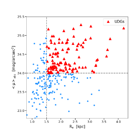
Figure 1: Mean surface brightness within circularized effective radius versus effective radius for all UDG candidates. In total, 108 UDGs are selected from the upper-right region, which are marked as red triangles. Blue circles are the rest of candidates.

2.3 GALFIT Fitting and Final Selection of UDGs

We use GALFIT (Peng et al., 2002, 2010) to fit the single Sérsic model (Sérsic, 1968) to each candidate. The fitting is done on $151\times 151$ pixels F814W images, which have been background-subtracted as described in Sec 2.2, but not PSF-matched. Before running galfit, we take use of the detection image from Noisechisel and the segmentation image from SExtractor to mask contamination pixels in the fields. This could help us to get robust fitting results. To avoid unreasonable fits, we restrict the ranges of Sérsic indices to be between 0.2 and 8 and those of the effective radii to be within 0.5 to 50 pixels. Examples of our fits are presented in Appendix.

Based on the best-fitting parameters from GALFIT models, we re-determine the effective radii and mean surface brightness of 285 UDG candidates more accurately. The distribution of their surface brightness versus radius are shown in Fig. 1. Finally, 108 candidates are confirmed to be our UDGs and are marked as red triangles in the top-right region of Fig. 1.

For reference, Table 2 lists the numbers of galaxies in each field after we apply different cuts to Shipley’s catalog. as well as the fraction of galaxies compared to the number of all detected sources in each cluster field.

Table 2: Numbers of galaxies after different cuts in this work.

Cluster	total	SB&Re cut (SEx-based)	photo-z cut	Visually Check	SB&Re cut (Galfit-based)
Abell2744	$9390$	$1872(19.94\%)$	$263(2.80\%)$	$56(0.60\%)$	$26(0.28\%)$
Abell370	$6795$	$1577(23.21\%)$	$163(2.40\%)$	$63(0.93\%)$	$23(0.34\%)$
AbellS1063	$7611$	$1726(22.68\%)$	$221(2.90\%)$	$80(1.05\%)$	$36(0.47\%)$
MACS0416	$7431$	$1600(21.53\%)$	$145(1.95\%)$	$37(0.50\%)$	$9(0.12\%)$
MACS0717	$6370$	$1460(22.92\%)$	$136(2.14\%)$	$21(0.33\%)$	$6(0.09\%)$
MACS1149	$6868$	$1715(24.97\%)$	$110(1.60\%)$	$28(0.41\%)$	$8(0.12\%)$

3 Results

3.1 Structural Properties

The histograms of Sérsic index and axis-ratios of the best-fitting GALFIT models are presented in panel (a) and panel (b) in Fig. 2, blue for all candidates while red for UDGs. Similar to UDGs in the local universe, UDGs in HFF fields have relative small n values and are not preferentially edge-on galaxies. In this work, 69% of UDGs have n smaller than 1.5 and the median value of n is 1.09, 82% of UDGs have b/a larger than 0.5 and the median value of b/a is 0.68. The statistics of Coma UDGs are 0.86 for n and 0.74 for b/a (Yagi et al., 2016). This means that current structural characteristics of local UDGs might be shaped earlier than z$\sim$0.4 and remain unchanged after a relatively long time ($\sim$ 3–5  Gyrs).

For galaxies having HST WFC3/IR coverage in HFF project, we run EAZY to get their rest-frame UVIJ magnitudes. Multi-band fluxes input to EAZY are based on our PSF-matched and background-subtracted images, input redshifts are fixed to be cluster redshifts. Rest-frame UVJ and UVI diagrams are shown in the panel (c) and panel (d) of Fig. 2, respectively. In our sample, 91 candidate galaxies and 14 UDGs have HST WFC3/IR data, they are marked as blue circles for candidate galaxies and red triangles for UDGs. Unlike cluster UDGs in the local Universe, which are found to be red in color and show no evidence of recent star forming activities, most of cluster UDGs in HFF populate the lower left region of UVJ and UVI diagrams in Fig. 2, which indicate that they are still star-forming. The relative blue rest-frame V - J colors ($V-J<1$) indicate that these UDGs contain small amount of dust content. By assuming all of our UDGs have relative small V - J color, we use rest-frame U - V color to investigate their star formation activity. Utilizing calibrations between rest-frame U - V and observed F606W - F814W in Wang et al. (2017), we calculate the rest-frame U - V colors for all 108 UDGs from their observed colors.

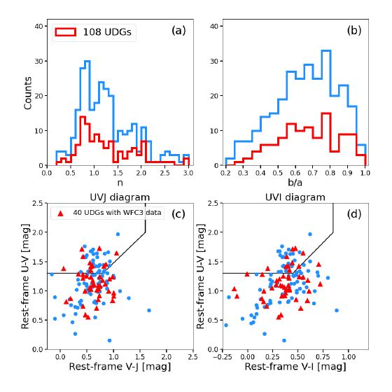
Figure 2: Statistics of basic properties of UDGs in this work. Panel (a) and (b) show histograms of the best-fitting Sérsic index n and b/a, respectively. UDGs are in red and all candidates are in blue. In Panel (c) and (d), we show the rest-frame UVJ and UVI diagrams for objects with HST WFC3/IR observations, whose rest-frame colors are obtained from the EAZY. In this work, 129 of 285 candidate galaxies and 40 of 108 UDGs have WFC3/IR data.

3.2 Radial Color Profiles

For each UDG, we estimate the mean surface brightness within a sequence of elliptical annuli. The parameters of annuli are taken from the best-fit GALFIT model of a UDG and they are applied to every band, During the computation, we fix the parameters for annuli from inside to outside. In Fig. 3, there is an example show our results on multi-band surface brightness profiles of UDGs. Panels (7) to (9) are PSF-matched background-subtracted cutout-images in F606W, F814W and F160W bands. The surface brightness in each band is calculated within the region between two neighboring colored ellipses. The final surface brightness profile is presented in panel (10). In panel (11), referring to Fig. A1 and Fig. A2 in Wang et al. (2017), we obtain the rest-frame U - V and V - I color profiles from observed F606W - F814W and F814W - F160W profiles, empirically. The shaded regions in panel (10) and panel (11) indicate the half of FWHM of PSF in F160W band, and the gray lines show the effective radii along semi-major axis. In panel (12), we exhibit rest-frame U - V versus V - I colors for all annuli. Figures for other 13 UDGs with WFC3/IR data are presented in the Appendix. Similar figures for a full version of all 108 UDGs could be found here (https://drive.google.com/file/d/1dmYcVn0zOi07R4WOXbxh7yNZ_GTKK623/view?usp=sharing).

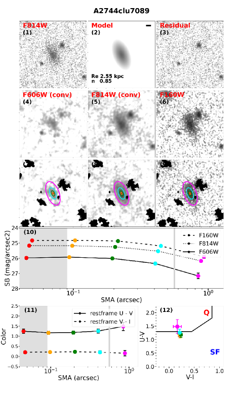
Figure 3: Example multi-band surface bright- ness profiles fitting for UDG A2744clu7089. Panels (1) to (3) show the F814W band cutout-images of the UDG, the best-fitting GALFIT model and residual image. The bar at top-right of panel (2) represents 1.5 kpc assuming the cluster redshift. Panels (4) to (6) show PSF-matched images in F606W, F814W and F160W bands. In panels (7) to (9), we mask neighboring sources classified by ‘Noisechisel’ and overplot our elliptical annuli used in surface brightness analysis. Panel (10) presents three-band surface brightness profiles of UDG A2744clu7089, x-axis of colorful points correspond to the out-radius of elliptical annuli. In panel (11), we convert observed color profiles into rest-frame U - V and V - I profiles. F814W and F160W surface brightness profiles in panel (10) and rest-frame V - I profiles in panel (11) are shifted a bit to the right. Finally, the colors of the UDG from inside to outside are shown in the UVI diagram in panel (12).

It can be seen that these HFF UDGs do not show significantly large color gradients within their effective radii, except for UDG AS1063clu2960. Meanwhile, there is a large fraction of UDGs that are undergoing star formation activities from inside to outside. These findings suggest that UDGs in distant clusters generally grow at a uniform rate throughout the galaxy.

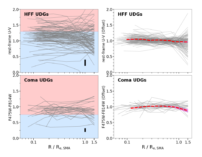
Figure 4: The radial color profiles of HFF UDGs and Coma UDGs. In the left two panels, the rest-frame U - V color profile of 108 HFF UDGs and HST F475W - F814W color profiles of Coma UDGs are presented, respectively. Blue and red backgrounds are used to show the classical separation for blue and red galaxies, the boundary we used here is 1.3 mag for the rest-frame U - V color and 0.76 mag for F475W - F814W color. Here 0.76 mag is the traditional g - i color of cluster UDGs, Coma UDGs are known to be red and quenched, our F475W - F814W profiles show that, Coma UDGs are red from inside to outside and have little color gradients. The typical uncertainty of the color near $\sim$ 1 * $R_{e,SMA}$ is 0.2 mag for HFF UDGs and 0.12 mag for Coma UDGs, which are shown as black bars, respectively. In the right two panels, we offset each color profile in the left two panels by letting its data points have an average value equal to 1. The median curve and corresponding 1-sigma uncertainty for the shifted color profiles is shown as red dashed line.

4 Discussions

4.1 Comparison with UDGs in the Coma Cluster

Lots of UDGs have been identified in Coma cluster, these Coma UDGs are found to be red and have old stellar population. Benefiting from the HST/ACS Coma Cluster Treasury Survey (Carter et al., 2008; Hammer et al., 2010), which provides deep and high resolution images in F475W and F814W bands, we do similar analysis for Coma UDGs selected from Yagi et al. (2016) catalog. Since the Coma UDGs usually have much larger angular size than the size of HST PSF, we do not match cutout-images to have the same PSF but only carefully subtract the background, set the $SMA$ of the innermost annulus for Coma UDGs are always begin at r = 7 pixel, beyond which we need not worry about the PSF effect.

The comparison of color profiles between HFF UDGs and Coma UDGs are shown in Fig. 4. For HFF UDGs, in left panel, we present the rest-frame U - V profiles of all 108 UDGs. In right panel, we offset each U - V profile by a mean distance of all annuli colors from ‘y = 1’, the median curve are plotted as red dashed line, magenta region show the 1–sigma uncertainties. For Coma UDGs, we do similar analysis on F475W - F814W profiles. Within the range of $0.1*R_{e,SMA}$ to $1.5*R_{e,SMA}$, both HFF UDGs and Coma UDGs have very small color gradients, the changes in color are smaller than 0.1 magnitude. Combining the lack of color gradients in both samples with the fact that two samples have very different colors (are starforming and quenched) indicates that cluster UDGs may fade or quench in a self-similar way in less than $\sim$ 4 Gyrs.

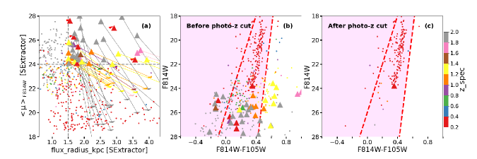
Figure 5: Panel (a) shows objects which have spectroscopic redshifts in Abell 2744 cluster field. They are plotted in the mean surface brightness versus effective radius space. Their surface brightness and radius are calculated by assuming the cluster redshift, using parameters from SExtractor. Triangles in the upper right region represent galaxies having low surface brightness and extened sizes under such assumption, their true values of surface brightness and half-light radius are shown with the arrow. In panel (b), the same sample is plotted in the F814W versus F814W - F105W space, two red dashed lines show boundaries of the ’red sequence’, the shaded region is where Lee et al. (2017, 2020) select their final UDGs. Panel (c) is a copy of panel (b), but applying the photo-z cut we used in this paper for Abell 2744 cluster. Each object is colored by their spectroscopic redshift.

4.2 Accuracy of Cluster Member identification

One of the biggest problems in identifying distant UDGs is their redshift/distance information, without which it is difficult to correctly determine their absolute magnitudes, unbiased surface brightness correction for the cosmic dimming effect, physical sizes, etc..

Since it has been known that UDGs in fields have quite different star formation activities from UDGs in clusters in the local universe, it would be important to select a relatively clean sample of UDGs in distant clusters with less background and foreground objects. Although spectroscopic observations are the most secure way to determine distances and cluster membership, they are too expensive to work for a large sample of distant UDGs. For instance, Kadowaki et al. (2021) reported that $\sim$ 1 hour exposure time on 10 m class telescopes often fails to yield a redshift for a candidate UDG in the Coma region. Previous studies utilized the color-magnitude diagram, Lee et al. (2017, 2020) kick out candidates which have color redder than the ’red sequence’ of bright cluster galaxies to get rid of background sources. This method definitely helps to remove background candidates from the sample, but how good is it?

In panel (a) of Fig. 5, we show the distribution of galaxies, which have spectroscopic redshifts (z_spec) in Abell 2744 cluster field, in the surface brightness versus radius space. Spectroscopic redshifts of these galaxies are taken from Shipley et al. (2018), which come from five liternature catalogs (see their Section 5.1 for details). The surface brightenss and half-light radii of these galaxies are calculated using the SExtractor parameters, by assuming they have the same redshift as the target cluster, just like what previous works did to select UDG candidates (Janssens et al., 2017, 2019; Lee et al., 2017, 2020). Galaxies in the upper-right region of panel (a) have surface brightness fainter than 24 $mag/arcsec^{2}$ in this way, but the true surface brighntness determined with their spec-z are much brighter and are shown with arrows. In panel (b) of Fig. 5, we show all z_spec-confirmed objects in the F814W versus F814W-F105W space, red dashed lines show the boundaries of the ‘red sequence’, which are used in Lee et al. (2017). It can be seen that simply removing objects redder than the ‘red sequence’ can help to remove some background galaxies, but the remaining sample still suffer from the contamination of a large fraction of interlopers. In panel (c) of Fig. 5, we present the result after applying our photo-z cut to this sample. It is clearly that, with the help of photometric redshifts, the majority of backgroud interlopers can be removed successfully, It should be noted that in this work we utilize photometric redshifts to effectively remove the background and foreground contaminants, but meanwhile, the sample size reduces. However, the sample purity is critically important for this study. In addition, applying a narrow range of photo-z cut is also crucial to correctly estimate the mean surface brightness and physical radius of sample galaxies, otherwise, the results could be far from the truth, as shown in panel (a) of Fig. 5.

We also utilize the XDF as a comparison to estimate the potential contributions of field UDGs or background galaxies to our cluster UDG sample. The XDF area we used cover $\sim 11$ arcmin², which are downloaded from the webpage https://archive.stsci.edu/prepds/xdf/. Photometric redshifts we used are from CANDELS team (Santini et al., 2015). We re-do our UDG selection process for the XDF. Referring to the redshift of each HFF cluster, we apply the same redshift cut for XDF galaxies. As a result, no UDGs are found in the XDF for the redshift of M0416, one UDG is found for the redshifts of Abell2744, Abell370 and AS1063, while two UDGs are seen in the XDF for the redshifts of M0717 and M1149. The findings indicate that the number density of potential interlopers in our selected UDGs from the six HFF clusters is very low ($0/0.1/0.2$ per arcmin² for one specific field).

4.3 Uncertainties in Photometric Redshifts

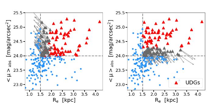
Figure 6: The diagram demonstrate the uncertainties in our sample selection. In left panel, we marked UDGs with gray triangles which will not be classified as UDGs when they are at redshifts equal to z_clu-0.1. The right panel show cases when UDGs are assumed to have their redshifts equal to z_clu-0.1.

In this work, we use photometric redshifts to select cluster members and our UDG sample, but the uncertainties in photometric redshifts produce uncertainties in surface brightness and physical radius of galaxies, which will make UDGs move out from the upper-right space in Fig.1. In this section, we simply evaluate this effect. In Sec.2.1, we apply $|$z_peak$\,-\,$z_clu$|\,<0.1$ to select cluster members. Referring to Shipley et al. (2018), around 80% of our candidate UDGs are located within this redshift range. But $\pm$ 0.1 uncertainty in redshift is not so accurate, which would introduce large uncertainties in the estimations of both surface brightness and radius when we select candidate UDGs. We re-estimate the surface brightness and radius of our UDGs under two conditions, assuming they have redshifts equal to z_clu-0.1 or z_clu+0.1. Objects which will not be classified as UDGs are marked with gray triangles in two differnt panels in Fig.6, separately. The gray arrows show where they will go. Two thirds of galaxies in our UDG sample will still satisfy the definition for UDGs if we assume a redshift of z_clu-0.1, and half of our UDGs will survive for z_clu+0.1. The uncertainty in photometric redshifts and the resulting changes in UDG sample sizes do not influence our main conclusions.

4.4 Completeness of our UDG sample

We run image simulations to evaluate the completeness of our UDG sample. Firstly, we use GALFIT to generate mock images in F814W band for each cluster, each mock image has a size of 151x151 pixels. Model parameters are chosen in the following way: Sérsic index is fixed to be n = 1. Circularized half-light radius is randomly chosen from a uniform distribution with a range of $1.5<R_{e}<7.5$ kpc. Total magnitude is randomly chosen from a uniform distribution with a range of $22<mag<29.5$ mag. Axis-ratio is set to follow a gaussian distribution with mean value of 0.7 and scatter value of 0.1, axis-ratio values lager than 1 or smaller than 0.1 will be fixed to be 1 or 0.1, respectively. As for position angle values, we just choose from 0-360 degrees, randomly. We generate 10000 model galaxies for each cluster and compute their absolute surface brightness as the same way we did for observed data. Only mock images who have $24<\langle\mu\rangle_{abs}<28$ mag/arcsec² will be used for the next step. In general. we will have $\sim$6400 mock UDGs for each cluster.

Secondly, we inject these mock UDGs into HFF F814W band images. To avoid an overcrowding in the simulations, we randomly pick up $\sim$40 mock galaxies from mock galaxy sample each time. For each cluster field, we run 500 simulations. We take use of the segmentation image to reduce the posibility of overlaping with other sources.

Lastly, we use SExtractor to detect these mock UDGs, an matching radius of 3 pixel is applied. The completeness map of absolute surface brightness versus. effective raidus for each HFF cluster is shown in Fig. 7. The completeness here is defined as a ratio of the number of detected UDGs to the number of injected UDGs. For UDGs with surface brightness brighter than 25.3 mag/arcsec² (the dimmest UDG in this work has a surface brightness of 25.3 mag/arcsec²), the completeness in all six clusters are better than 80%.

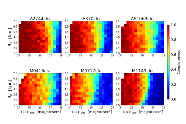
Figure 7: Completeness maps as a function of size and surface brightness for n=1 Sérsic profiles.

4.5 Concerns of UDG sample size compared with previous works

Lee et al. (2017, 2020) identified 27 UDGs in A2744 cluster field, 34 UDGs in A370 cluster field and 35 UDGs in AS1063 cluster field, whereas the numbers of UDGs we found from these fields are 26,23 and 36, respectively. Two works found similar numbers of UDGs from these three clusters. Janssens et al. (2019) found more UDGs than our work, and in particular the numbers of UDGs they found in three more distant clusters, MACS0416, MACS0717 and MACS1149, are comparable to those in other three clusters. However, the number of UDGs we found from MACS0416, MACS0717 and MACS1149 are far less than the other three clusters. To check this, we especially loosen the selection criteria of UDG candidates in Section 2.1 to be $\langle\mu_{F814W}\rangle$  $\textgreater\,22.5mag/arcsec^{2}$ and flux_radius_kpc $\textgreater$ 1.0 kpc, and re-do our sample selection process. As a result, the sample size of final UDGs in the six cluster fields increases to 131, of which four are in MACS0416, four in MACS0717 and two in MACS1149. Main results and conclusions we have drawn remain unchanged when using this enlarged sample of candidate UDGs.

The differences of sample sizes between this study and previous works primarily result from applying a narrow photo-z cut during our selection process. In Lee et al. (2017, 2020), they did not apply any photo-z cut to their sample. In Janssens et al. (2019), they just restricted their candidates to have photo-z less than 1. We cross-match selected 27 UDGs in A2744 by Lee et al. with the catalog of Shipley et al. (2018) to obtain 25 UDGs with photo-z measurement. If we apply the same photo-z cut used in this work to these 25 UDGs of Lee et al, only 8 UDGs will pass the photo-z cut. The result indicates that the UDG sample of Lee et al may be more affected by foreground/background interlopers than initially thought.

It has been proposed that UDGs are born primarily in the field, later processed in groups and, ultimately, infall into galaxy clusters (e.g., Román & Trujillo, 2017). Using large simulations, Rong et al. (2017) found that UDGs could be a type of dwarf galaxies residing in the low-density regions hosted by large spin halos, which fell into the clusters with a median infall time of $\sim$8.9 Gyr, corresponding to a redshift of 0.43. Tremmel et al. (2020) also showed that UDGs in cluster environments form from dwarf galaxies that experienced early cluster in-fall and subsequent quenching. Bachmann et al. (2021) showed that distant UDGs in clusters are relatively under-abundant, as compared to local UDGs, by a factor $\sim 3$.

In Fig. 8, we show the surface densities of UDGs in HFF clusters as a function of redshift. The density value of each cluster is computed with the following formula:

$$\sum=\frac{\sum_{n}^{N_{UDGs,clu}}1/comp_{n}}{Area_{clu}}$$ (3)

Here, $N_{UDGs,clu}$ is the number of UDGs in each cluster. $comp_{n}$ is the completeness value, which is determined from Fig. 7 according to the surface brightness and effective radius of each UDG. $Area_{clu}$ is the coverage area of HFF cluster field in F814W band, they are from the Table 1 of Shipley et al. (2018). The result of completeness-corrected surface number densities of UDGs ($\sum$) is shown in the left panel of Fig. 8 (black points). There is an obvious difference of $\sum$ between clusters at higher redshift and lower redshift. van der Burg et al. (2016) found that the abundance of UDGs are correlated with the virial mass of host clusters . In the right panel of Fig. 8, we calibrate $\sum$ with the M200 of each cluster. Here, we adopt the same M200 values for HFF clusters as listed in Table 1 of Janssens et al. (2019). The M200-calibrated $\sum$ of clusters at z$\sim$0.55 is smaller than those at $z<0.4$, the difference is greater than 0.55 dex (black points). Considering object will look dimmer when it is put at a high redshift due to cosmic dimming effect, the difference of surface number densities of UDGs shown with the black points in Fig. 8 could be a result of systematic effect. In order to check this, we compute surface number densities only for bright UDGs ($\langle\mu\rangle_{abs}<24.5$), the results are plotted with red cross in Fig. 8. The limit of 24.5 we used here is close to the faitest UDG we found in two $z\sim 0.55$ clusters MACS0717 and MACS1149, above this level, our UDGs have completeness greater than 90%, The difference in surface number densities for bright UDGs between high-z clusters (z$\sim$0.55) and low-z clusters ($z<0.4$) still exists. Based on Rong et al. (2017)’ simulation, cluster UDGs can be from the infall of field-born UDGs, and the median infall time predicted in their work is $\sim$8.9 Gyr (corresponding to $z\sim 0.43$). The lack of UDGs in clusters MACS0717 and MACS1149 could be a result that few UDGs have fell into dense environment at $z>0.4$, though large uncertainties exist. Further exploration with better observations is needed in the future.

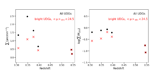
Figure 8: Surface number densities of UDGs in HFF clusters as a function of redshift. Left panel shows the completenes-corrected values and right panel shows the cluster-mass-calibrated $\&$ completeness-corrected values, the unit of y-axis in two panels are $arcmin^{-2}$ and log[$arcmin^{-2}*10^{-15}M_{sun}$] from left to right. Black points and red crosses show the surface number densities computed using all UDG sample and bright UDGs ($\langle\mu\rangle_{abs}<24.5$), respectively.

5 Summary

We carefully identify 108 UDGs from six distant massive galaxy clusters in the HFF in redshift range from 0.308 to 0.545. We measure their structral parameters using GALFIT and their radial rest-frame color profiles, and make a comparison with UDGs in the Coma cluster. We show that the HFF UDGs have a median Sérsic index of 1.09, which is close to 0.86 for Coman UDGs. The median axis-ratio value is 0.68 for HFF UDGs and 0.74 for Coma UDGs, respectively. We find that UDGs in the HFF do not show significantly large color gradients within their effective radii. Changes from inside to outside of the median color profile are smaller than 0.1 magnitudes. Meanwhile, unlike UDGs in the Coma cluster, whose color profiles are mostly red from inside to outside, a large fraction of HFF UDGs have blue colors and are star-forming. Our findings provide evidence that UDGs in clusters may have a self-similar star formation quenching mode when evolving from distant to the local universe. Besides, we find the M200-calibrated surface number densities of UDGs is lower at two $z\sim 0.55$ clusters when comparing to other HFF clusters. Under the scenario that UDGs might be born in the field and finnally infall into galaxy clusters (Román & Trujillo, 2017), the lack of UDGs found in distant clusters imply that few UDGs have fell into dense environment at $z>0.4$, which agrees with the simulation work from Rong et al. (2017).

Table 3: Catalog of 108 UDGs identified in the HFF program

ID	$R.A.(J2000)$	$Dec.(J2000)$	$<\mu>$	$R_{e,SMA}$	n	q	rest-frame U-V
A2744clu0112	3.5817	-30.4312	24.28	2.0	1.1	0.4	0.85
A2744clu0448	3.5952	-30.4228	24.88	1.64	0.95	0.79	0.56
A2744clu0679	3.5912	-30.4194	24.91	1.94	1.31	0.58	2.14
A2744clu0745	3.5787	-30.4188	24.75	2.71	1.72	0.58	1.22
A2744clu1656	3.6062	-30.4116	24.11	2.43	0.71	0.34	0.69
A2744clu1717	3.616	-30.4107	24.98	2.44	1.58	0.64	0.91
A2744clu2029	3.5748	-30.4095	24.83	2.22	1.36	0.55	1.36
A2744clu2489	3.5596	-30.4065	25.13	2.1	0.75	0.54	1.39
A2744clu2651	3.6231	-30.406	24.54	1.9	0.79	0.72	0.64
A2744clu4431	3.5648	-30.397	24.99	1.69	1.05	0.97	1.17
A2744clu5026	3.5641	-30.3944	24.65	1.82	0.79	0.78	0.59
A2744clu5159	3.5638	-30.3935	24.99	1.75	0.79	0.72	1.33
A2744clu6355	3.6024	-30.387	24.16	1.81	3.0	0.89	1.1
A2744clu6625	3.5822	-30.3849	24.37	3.28	1.93	0.34	1.05
A2744clu7053	3.5634	-30.3815	25.17	1.56	0.79	0.87	0.66
A2744clu7089	3.5835	-30.3822	24.63	2.55	0.85	0.49	1.37
A2744clu7219	3.5665	-30.3806	24.11	1.72	1.29	0.8	0.52
A2744clu7257	3.5641	-30.3817	24.03	3.15	1.23	0.76	1.06
A2744clu7651	3.5914	-30.3774	24.53	1.8	1.04	0.86	1.31
A2744clu7696	3.5907	-30.3772	24.63	3.62	0.84	0.55	0.68
A2744clu8134	3.5762	-30.3718	24.18	1.69	0.75	0.7	0.87
A2744clu8312	3.6025	-30.3695	24.15	1.84	1.31	0.72	0.6
A2744clu8655	3.5908	-30.3638	24.27	1.78	1.73	0.43	1.21
A2744clu8657	3.595	-30.3638	24.49	1.62	1.81	0.79	0.86
A2744clu8681	3.5853	-30.3644	24.22	3.22	1.55	0.43	0.9
A2744clu8818	3.5899	-30.3622	24.34	3.24	1.08	0.9	1.04
A370clu0353	39.9598	-1.6067	24.81	2.78	0.59	0.91	0.27
A370clu0459	39.9636	-1.6043	24.1	1.84	0.82	0.51	1.08
A370clu0646	39.9604	-1.6014	24.11	2.18	1.62	0.52	0.74
A370clu0896	39.9838	-1.5979	25.2	4.19	1.94	0.6	0.75
A370clu1046	39.9821	-1.5958	24.16	2.64	1.67	0.4	1.26
A370clu1456	39.9851	-1.5917	24.12	2.3	1.14	0.52	0.67
A370clu1760	39.9958	-1.5885	24.15	1.7	1.23	0.68	1.53
A370clu2123	39.9822	-1.5854	25.25	3.04	1.11	0.61	1.02
A370clu2258	39.9887	-1.5837	24.93	3.03	0.65	0.67	1.65
A370clu2416	39.9451	-1.5827	24.38	2.11	1.29	0.63	1.48
A370clu2512	39.9897	-1.582	24.17	1.69	2.08	0.59	1.65
A370clu2569	39.9863	-1.582	24.07	2.09	1.33	0.84	1.01
A370clu3299	39.9402	-1.5762	24.51	1.82	0.94	0.89	0.87
A370clu3386	39.9506	-1.5754	24.13	1.66	0.69	0.51	0.75
A370clu3876	39.9615	-1.573	24.28	2.01	0.73	0.91	0.9
A370clu3936	39.941	-1.5714	24.04	1.65	1.12	0.75	0.83
A370clu3999	39.9523	-1.5708	24.27	1.72	0.95	0.56	1.15
A370clu4169	39.9545	-1.5696	24.28	1.97	2.07	0.7	0.87
A370clu4746	39.9717	-1.5646	24.44	1.7	2.14	0.89	0.82
A370clu4938	39.9344	-1.5626	24.2	2.32	0.62	0.56	0.76
A370clu5038	39.9491	-1.5621	24.45	3.58	1.36	0.39	1.25
A370clu5094	39.9827	-1.5611	24.07	1.55	1.84	0.58	0.6
A370clu5325	39.9841	-1.559	24.14	1.75	1.41	0.86	1.26
AS1063clu0008	342.178	-44.5698	24.89	2.23	1.92	0.88	0.89
AS1063clu0224	342.1824	-44.5616	25.29	2.7	1.86	0.74	0.71
AS1063clu0288	342.1791	-44.5603	24.05	1.65	1.83	0.72	1.15
AS1063clu0308	342.175	-44.56	24.34	1.71	0.8	0.42	0.26
AS1063clu0379	342.1697	-44.5584	24.03	1.88	1.1	0.43	1.11
AS1063clu0496	342.1641	-44.5562	24.19	1.79	0.88	0.26	0.71
AS1063clu1208	342.17	-44.5469	24.53	1.86	1.55	0.69	0.59
AS1063clu1228	342.1644	-44.5464	24.16	1.64	1.3	0.5	1.07
AS1063clu2393	342.199	-44.5381	24.25	2.19	0.93	0.52	1.3
AS1063clu2427	342.1948	-44.538	24.22	1.93	0.73	0.76	1.06
AS1063clu2749	342.2347	-44.5355	24.81	1.93	0.82	0.57	1.16
AS1063clu2812	342.1494	-44.5352	24.1	1.73	2.0	0.91	1.56
AS1063clu2960	342.203	-44.5349	24.67	1.57	0.78	0.95	0.43
AS1063clu3056	342.1991	-44.5344	24.63	2.05	0.71	0.59	0.79
AS1063clu3122	342.1441	-44.5336	24.79	2.42	1.28	0.78	1.04
AS1063clu3242	342.2192	-44.5329	24.25	1.88	0.35	0.45	0.81
AS1063clu3267	342.1437	-44.5332	24.2	3.21	0.87	0.46	0.73
AS1063clu3377	342.2192	-44.5322	24.82	2.04	0.87	0.7	1.49
AS1063clu3447	342.2319	-44.532	24.25	2.14	1.17	0.6	1.43
AS1063clu3471	342.2271	-44.5318	24.65	2.27	0.97	0.76	1.1
AS1063clu3607	342.217	-44.531	25.18	2.44	0.56	0.44	-0.45
AS1063clu3937	342.2027	-44.5308	24.73	2.57	1.75	0.79	2.07
AS1063clu4009	342.1379	-44.5295	24.12	1.57	1.01	0.7	0.74
AS1063clu4519	342.2163	-44.5273	24.02	1.59	0.96	0.94	1.27
AS1063clu4855	342.1356	-44.5254	24.16	2.16	1.34	0.81	0.72
AS1063clu4972	342.1483	-44.5243	24.52	1.73	1.1	0.6	1.12
AS1063clu5030	342.1747	-44.5249	24.8	1.78	1.54	0.92	0.84
AS1063clu5710	342.1502	-44.5194	24.56	2.21	0.87	0.76	0.73
AS1063clu5943	342.1656	-44.5179	24.78	2.61	2.57	0.7	1.04
AS1063clu6074	342.1734	-44.5171	24.7	2.76	2.9	0.76	1.1
AS1063clu6396	342.1882	-44.5143	24.08	2.03	0.75	0.91	1.1
AS1063clu6652	342.1866	-44.5171	24.08	1.97	2.27	0.84	1.45
AS1063clu6653	342.1972	-44.5108	24.81	2.18	0.47	0.63	1.66
AS1063clu6721	342.1967	-44.5102	24.82	1.66	0.69	0.75	0.6
AS1063clu6800	342.1955	-44.5095	24.04	2.23	0.7	0.94	0.62
AS1063clu7141	342.1833	-44.5037	24.9	2.86	0.75	0.69	1.32
M0416clu0656	64.0465	-24.095	24.01	1.56	0.87	0.62	0.92
M0416clu0666	64.045	-24.0954	24.24	2.27	2.05	0.57	0.9
M0416clu0833	64.0661	-24.0925	24.71	1.51	0.57	0.75	1.13
M0416clu1090	64.0126	-24.0899	24.04	1.66	1.04	0.64	0.89
M0416clu4132	64.0078	-24.0707	24.32	1.52	2.08	0.71	1.01
M0416clu5295	64.0575	-24.0643	24.1	1.97	0.69	0.66	1.21
M0416clu5483	64.0241	-24.0627	24.01	1.62	0.96	0.84	1.11
M0416clu6651	64.0572	-24.0532	24.65	2.24	0.3	0.54	1.2
M0416clu6894	64.0427	-24.0504	24.91	3.71	0.82	0.64	1.07
M0717clu0069	109.4029	37.7197	24.13	2.51	1.76	0.44	1.22
M0717clu0456	109.42	37.7254	24.01	1.68	1.0	0.62	1.78
M0717clu1415	109.3851	37.7338	24.06	3.09	1.15	0.98	1.46
M0717clu5158	109.3811	37.7647	24.19	1.75	2.4	0.65	0.66
M0717clu5661	109.3872	37.7699	24.16	2.85	1.2	0.91	1.19
M0717clu5958	109.3839	37.7733	24.27	2.48	0.83	0.77	0.66
M1149clu0324	177.4102	22.3731	24.09	2.4	2.02	0.85	0.71
M1149clu0541	177.4016	22.3764	24.43	2.63	0.35	0.48	1.0
M1149clu0778	177.3933	22.3794	24.02	1.91	2.08	0.88	2.28
M1149clu3274	177.4119	22.398	24.15	2.76	1.03	0.62	1.31
M1149clu3831	177.3808	22.4017	24.46	1.89	2.38	0.65	0.52
M1149clu5184	177.4058	22.4106	24.29	2.15	0.87	0.66	0.7
M1149clu5625	177.3822	22.4142	24.04	2.4	1.89	0.39	1.09
M1149clu6156	177.4072	22.4199	24.06	2.56	2.69	0.47	1.2

Note. — Basic information of our 108 UDGs. Col ‘ID’ is the combined ID of cluster name and id from Shipley’s catalog. R.A.(J2000) and Dec.(J2000) are directly from Shipley’s catalog. $<\mu>$, $R_{e,SMA}$, n, q are structural parameters.

References

- Akhlaghi & Ichikawa (2015) Akhlaghi, M., & Ichikawa, T. 2015, ApJS, 220, 1
- Amorisco et al. (2018) Amorisco, N. C., Monachesi, A., Agnello, A., & White, S. D. M. 2018, MNRAS, 475, 4235
- Bachmann et al. (2021) Bachmann, A., van der Burg, R. F. J., Fensch, J., Brammer, G., & Muzzin, A. 2021, A&A, 646, L12
- Barden et al. (2012) Barden, M., Häußler, B., Peng, C. Y., McIntosh, D. H., & Guo, Y. 2012, GALAPAGOS: Galaxy Analysis over Large Areas: Parameter Assessment by GALFITting Objects from SExtractor, Astrophysics Source Code Library, record ascl:1203.002, , , ascl:1203.002
- Bertin & Arnouts (1996) Bertin, E., & Arnouts, S. 1996, A&AS, 117, 393
- Blanton et al. (2003) Blanton, M. R., Brinkmann, J., Csabai, I., et al. 2003, AJ, 125, 2348
- Brammer et al. (2008) Brammer, G. B., van Dokkum, P. G., & Coppi, P. 2008, ApJ, 686, 1503
- Carter et al. (2008) Carter, D., Goudfrooij, P., Mobasher, B., et al. 2008, ApJS, 176, 424
- Castellano et al. (2016) Castellano, M., Amorín, R., Merlin, E., et al. 2016, A&A, 590, A31
- Chilingarian (2009) Chilingarian, I. V. 2009, MNRAS, 394, 1229
- Conselice et al. (2002) Conselice, C. J., Gallagher, John S., I., & Wyse, R. F. G. 2002, AJ, 123, 2246
- Conselice et al. (2003) —. 2003, AJ, 125, 66
- de Rijcke et al. (2009) de Rijcke, S., Penny, S. J., Conselice, C. J., Valcke, S., & Held, E. V. 2009, MNRAS, 393, 798
- Gu et al. (2018) Gu, M., Conroy, C., Law, D., et al. 2018, ApJ, 859, 37
- Haigh et al. (2021) Haigh, C., Chamba, N., Venhola, A., et al. 2021, A&A, 645, A107
- Hammer et al. (2010) Hammer, D., Verdoes Kleijn, G., Hoyos, C., et al. 2010, ApJS, 191, 143
- He et al. (2019) He, M., Wu, H., Du, W., et al. 2019, ApJ, 880, 30
- Hogg et al. (2002) Hogg, D. W., Baldry, I. K., Blanton, M. R., & Eisenstein, D. J. 2002, arXiv e-prints, astro
- Iodice et al. (2020) Iodice, E., Cantiello, M., Hilker, M., et al. 2020, A&A, 642, A48
- Janssens et al. (2017) Janssens, S., Abraham, R., Brodie, J., et al. 2017, ApJ, 839, L17
- Janssens et al. (2019) Janssens, S. R., Abraham, R., Brodie, J., Forbes, D. A., & Romanowsky, A. J. 2019, ApJ, 887, 92
- Jerjen et al. (2000) Jerjen, H., Binggeli, B., & Freeman, K. C. 2000, AJ, 119, 593
- Kadowaki et al. (2017) Kadowaki, J., Zaritsky, D., & Donnerstein, R. L. 2017, ApJ, 838, L21
- Kadowaki et al. (2021) Kadowaki, J., Zaritsky, D., Donnerstein, R. L., et al. 2021, ApJ, 923, 257
- Koda et al. (2015) Koda, J., Yagi, M., Yamanoi, H., & Komiyama, Y. 2015, ApJ, 807, L2
- Koleva et al. (2011) Koleva, M., Prugniel, P., De Rijcke, S., & Zeilinger, W. W. 2011, MNRAS, 417, 1643
- Lee et al. (2020) Lee, J. H., Kang, J., Lee, M. G., & Jang, I. S. 2020, ApJ, 894, 75
- Lee et al. (2017) Lee, M. G., Kang, J., Lee, J. H., & Jang, I. S. 2017, ApJ, 844, 157
- Leisman et al. (2017) Leisman, L., Haynes, M. P., Janowiecki, S., et al. 2017, ApJ, 842, 133
- Liu et al. (2016) Liu, F. S., Jiang, D., Guo, Y., et al. 2016, ApJ, 822, L25
- Liu et al. (2017) Liu, F. S., Jiang, D., Faber, S. M., et al. 2017, ApJ, 844, L2
- Liu et al. (2018) Liu, F. S., Jia, M., Yesuf, H. M., et al. 2018, ApJ, 860, 60
- Lotz et al. (2017) Lotz, J. M., Koekemoer, A., Coe, D., et al. 2017, ApJ, 837, 97
- Merlin et al. (2016) Merlin, E., Amorín, R., Castellano, M., et al. 2016, A&A, 590, A30
- Mieske et al. (2007) Mieske, S., Hilker, M., Infante, L., & Mendes de Oliveira, C. 2007, A&A, 463, 503
- Mihos et al. (2015) Mihos, J. C., Durrell, P. R., Ferrarese, L., et al. 2015, ApJ, 809, L21
- Pagul et al. (2021) Pagul, A., Sánchez, F. J., Davidzon, I., & Mobasher, B. 2021, ApJS, 256, 27
- Peng et al. (2002) Peng, C. Y., Ho, L. C., Impey, C. D., & Rix, H.-W. 2002, AJ, 124, 266
- Peng et al. (2010) —. 2010, AJ, 139, 2097
- Penny et al. (2009) Penny, S. J., Conselice, C. J., de Rijcke, S., & Held, E. V. 2009, MNRAS, 393, 1054
- Penny et al. (2011) Penny, S. J., Conselice, C. J., de Rijcke, S., et al. 2011, MNRAS, 410, 1076
- Román & Trujillo (2017) Román, J., & Trujillo, I. 2017, MNRAS, 468, 4039
- Rong et al. (2017) Rong, Y., Guo, Q., Gao, L., et al. 2017, MNRAS, 470, 4231
- Rong et al. (2020) Rong, Y., Zhu, K., Johnston, E. J., et al. 2020, ApJ, 899, L12
- Sandage & Binggeli (1984) Sandage, A., & Binggeli, B. 1984, AJ, 89, 919
- Santini et al. (2015) Santini, P., Ferguson, H. C., Fontana, A., et al. 2015, ApJ, 801, 97
- Sérsic (1968) Sérsic, J. L. 1968, Atlas de Galaxias Australes
- Shi et al. (2017) Shi, D. D., Zheng, X. Z., Zhao, H. B., et al. 2017, ApJ, 846, 26
- Shipley et al. (2018) Shipley, H. V., Lange-Vagle, D., Marchesini, D., et al. 2018, ApJS, 235, 14
- Thompson & Gregory (1993) Thompson, L. A., & Gregory, S. A. 1993, AJ, 106, 2197
- Tremmel et al. (2020) Tremmel, M., Wright, A. C., Brooks, A. M., et al. 2020, MNRAS, 497, 2786
- Trujillo et al. (2017) Trujillo, I., Roman, J., Filho, M., & Sánchez Almeida, J. 2017, ApJ, 836, 191
- van der Burg et al. (2016) van der Burg, R. F. J., Muzzin, A., & Hoekstra, H. 2016, A&A, 590, A20
- van Dokkum et al. (2016) van Dokkum, P., Abraham, R., Brodie, J., et al. 2016, ApJ, 828, L6
- van Dokkum et al. (2015a) van Dokkum, P. G., Abraham, R., Merritt, A., et al. 2015a, ApJ, 798, L45
- van Dokkum et al. (2015b) van Dokkum, P. G., Romanowsky, A. J., Abraham, R., et al. 2015b, ApJ, 804, L26
- Venhola et al. (2017) Venhola, A., Peletier, R., Laurikainen, E., et al. 2017, A&A, 608, A142
- Villaume et al. (2022) Villaume, A., Romanowsky, A. J., Brodie, J., et al. 2022, ApJ, 924, 32
- Wang et al. (2017) Wang, W., Faber, S. M., Liu, F. S., et al. 2017, MNRAS, 469, 4063
- Wu et al. (2005) Wu, H., Shao, Z., Mo, H. J., Xia, X., & Deng, Z. 2005, ApJ, 622, 244
- Yagi et al. (2016) Yagi, M., Koda, J., Komiyama, Y., & Yamanoi, H. 2016, ApJS, 225, 11
- Zaritsky et al. (2021) Zaritsky, D., Donnerstein, R., Karunakaran, A., et al. 2021, ApJS, 257, 60