Hyperuniformity and number rigidity of inflation tilings

Abstract.

In this article we prove that a large class of inflation tilings are hyperuniform: this includes the novel hat tilings introduced by Smith et al. and well known examples such as Penrose, Ammann-Beenker and shield tilings. In some cases, such as for Penrose tilings, we are also able to prove number rigidity, making them the first aperiodic examples with finite local complexity, hyperuniformity and number rigidity in higher dimensions. We prove this by deriving self-similarity equations for spherical diffraction, which generalize renormalization relations for ordinary diffraction found by Baake and Grimm.

Our method applies to inflation tilings of arbitrary dimensions for which there is a sufficiently large eigenvalue gap in the reduced substitution matrix.

1. Introduction

1.1. Hyperuniformity and rigidity

In this article, we will be concerned with two aspects of long range order for inflation tilings, namely hyperuniformity and number rigidity.

A locally square integrable point process $\Lambda$ on $\mathbb{R}^{d}$ is said to be hyperuniform if $\frac{\operatorname{Var}(\#\Lambda\cap B_{R})}{R^{d}}\to 0$ as $R$ approaches infinity, where $B_{R}$ is the Euclidean ball of radius $R$ centered at the origin. We define $\Lambda$ to be number rigid if the number of points within $B$ is almost surely determined by the points outside of $B$.

Hyperuniformity was introduced in 2003 by Torquato and Stillinger [33], while the study of rigidity phenomena was initiated by Ghosh and Peres [17] [18]. These properties have been widely studied from the viewpoints of materials science, chemistry, and stochastic geometry: see Torquato [32] and Coste [14] for recent surveys of the current state of the art.

It was recently shown by Björklund and Hartnick [9] that there exist cut-and-project quasicrystals which are not hyperuniform, and may even be antihyperuniform. This is surprising, as quasicrystals are usually thought to be models of materials exhibiting aperiodic order, so one would assume they should be hyperuniform and number rigid. So far, hyperuniformity has been studied mostly for structures which don’t have aperiodic order in the typical sense, such as physical models of exotic gases, liquids and plasma: in comparison, there has been little research on hyperuniformity for quasicrystals or inflation tilings, specially beyond the one dimensional case. This is even more true when it comes to number rigidity: as far as we can tell, Björklund and Hartnick [9] are the only ones that have studied number rigidity for model sets, or other systems with aperiodic order.

In addition to cut-and-project sets, inflation tilings are also a very important method of construct systems with aperiodic order. Therefore, it is natural to ask: When are inflation tilings hyperuniform? When are they number rigid?

Extending the methods of Baake, Gähler, and Mañibo [7] and Fuchs, Mosseri, and Vidal [15], we will be able to prove:

Theorem 1.1.

Fibonacci, Penrose, Ammann-Beenker, shield, ABCK, CAP and hat tilings are hyperuniform. Fibonacci, Penrose and Ammann-Beenker tilings are also number rigid.

We summarize Theorem 1.1 in the following table.

Tiling	Properties	Example	Previous work
Fibonacci	HU, NR	5.14	Baake and Grimm [5]
Penrose	HU, NR	5.15	Fuchs, Mosseri, and Vidal [15]
Ammann-Beenker	HU, NR	5.15	Fuchs, Mosseri, and Vidal [15]
Shield	HU, NR	5.16	New
ABCK	HU	5.17	New
CAP	HU	5.18	New
Hat	HU	5.18	New

Table 1. Hyperuniformity (HU) and number rigidity (NR) for many examples

(a) A Penrose tiling

(b) An AB tiling

(c) A Hat tiling

Figure 1. Some of the tilings mentioned in Theorem 1.1

We will focus on tilings coming from inflation systems, which are among the most studied structures exhibiting aperiodic order. An inflation system is characterized by a scaling constant $\lambda>0$, a finite set of prototiles $F=\{t_{1},\cdots,t_{\ell}\}$, and an inflation rule $\varrho$. We will focus on inflation tilings where $\ell\geq 2$, meaning that there are at least two protototiles: we will adress the case $\ell=1$ in a subsequent work.

From this data, assuming some technical conditions, one can construct “inflation tilings” associated to them, such that the inflation rule describes a certain “scale symmetry” of the tiling. Also essential is its inflation matrix $A\in\mathbb{R}^{\ell\times\ell}$, a positive matrix which encodes many important properties of the inflation rule, and has $\lambda^{d}$ as its largest eigenvalue.

Theorem 1.1 is a direct consequence of the following result (technical terms will be defined later):

Theorem 1.2.

Let $\mathcal{S}$ be an inflation system in $\mathbb{R}^{d}$ which is primitive, has finite local complexity and pure point powder diffraction. Let $\Lambda_{T}$ be the associated point process, $\lambda$ be the scaling constant and $\rho_{2}$ the absolute value of the second-largest eigenvalue of the reduced inflation matrix.

1. If $\rho_{2}<\lambda^{d/2}$, then $\Lambda_{T}$ is hyperuniform.

2. If $\rho_{2}<1$, then $\Lambda_{T}$ is also number rigid.

Theorem 1.2 can be obtained by using spectral methods as follows: let $\Lambda$ be a locally square integrable point process on $\mathbb{R}^{d}$. To it one can associate a diffraction measure $\hat{\eta}$, given as the Fourier transform (see [23]) of the autocorrelation measure of $\Lambda$. Let $\underline{h}(\Lambda)=\underline{\lim}_{r\to\infty}\frac{\log{\hat{\eta}(B_{r}-\{0\})}}{\log r}$ be the lower degree of uniformity of $\Lambda$. Then hyperuniformity and number rigidity can be characterized in terms of $\underline{h}$ as follows:

Theorem 1.3.

Let $\Lambda$ be a locally square integrable point process in $\mathbb{R}^{d}$. Then:

1. If $\underline{h}(\Lambda)>d$, then $\Lambda$ is hyperuniform

2. If $\underline{h}(\Lambda)>2d$, then $\Lambda$ is number rigid

To be able to apply this to inflation tilings, we will need the two following tools:

• The concept of renormalization relations for inflation tilings, developed by Baake and Gähler [3] (see also Baake, Gähler, and Mañibo [7])

• The use of powder diffraction, a notion of diffraction obtained by averaging rotationally. This has been studied by Baake, Frettlöh, and Grimm [6] among others, but our particular approach is informed by the concept of spherical diffraction, which can be defined in much greater generality and has been applied to aperiodic order by Björklund, Hartnick, and Pogorzelski [12].

Both of these follow from well known variance arguments for hyperuniformity and rigidity: see Coste [14] for a survey of the topic. In the literature, it is often assumed that the diffraction is continuous, but this assumption is not necessary: see Björklund and Hartnick [9, Theorem 1.1, Lemma 7.3] for a proof for general locally square integrable point process.

1.2. Colored point processes and diffraction matrices

We have already mentioned that, given an inflation system, we can associate to it a point process $\Lambda$. However, for us, it will be important to keep track of the different kinds of tiles in a tiling. If $\mathcal{S}$ is an inflation system with prototiles $F=\{t_{1},\cdots,t_{\ell}\}$, we define the colored point process associated to $\mathcal{S}$ as the random vector of point sets $\boldsymbol{\Lambda}=(\Lambda_{1},\cdots,\Lambda_{\ell})$, where $\Lambda_{i}$ includes only tiles which are translates of the prototile $t_{i}$.

There are many ways to obtain a point process from $\boldsymbol{\Lambda}$: for example, one can consider the individual processes $\Lambda_{i}$ or the union $\dot{\cup}\Lambda_{i}$. If one identifies a discrete set of points with the measure given by its Dirac comb, one can consider arbitrary linear combinations $w^{T}\boldsymbol{\Lambda}=\sum_{i=1}^{\ell}w_{i}\Lambda_{i}$, which are still locally square integrable random pure point measures, and therefore point processes (note that we allow point processes where the atoms do not necessarily have measure $1$: sometimes these are called “weighted point processes”). When we say a colored point process is hyperuniform or number rigid we mean that every linear combination is.

If $\boldsymbol{\Lambda}$ is a colored point process, one can define its diffraction matrix $\hat{\boldsymbol{\eta}}$, which is a matrix of measures such that the coefficients $\hat{{\eta}}_{ij}$ are the Fourier transforms of the autocorrelation between points with label $i$ and points with label $j$. Given the diffraction matrix of $\boldsymbol{\Lambda}$, one can recover the diffraction of any linear combination $w^{T}\boldsymbol{\Lambda}=\sum_{i=1}^{\ell}w_{i}\Lambda_{i}$ as $w^{T}\hat{\boldsymbol{\eta}}w=\sum_{i,j=1}^{\ell}w_{i}w_{j}\hat{{\eta}}_{ij}$. Therefore, if we let $\underline{h}(\boldsymbol{\Lambda})=\underline{\lim}_{r\to\infty}\frac{\log{\lVert\hat{\boldsymbol{\eta}}\rVert(B_{r}-\{0\})}}{\log r}$ we have $\underline{h}(\boldsymbol{\Lambda})\geq\underline{h}({w^{T}\boldsymbol{\Lambda}})$, so we can also use $\underline{h}(\boldsymbol{\Lambda})$ to find out whether $\boldsymbol{\Lambda}$ is hyperuniform or not.

1.3. Classical renormalization

One of the core tools we use in this article is the concept of renormalization. The broad idea of renormalization is as follows: if a tiling has some kind of self-similarity, quantities associated to it, will also be “self-similar” in a certain way. This means that the autocorrelation and diffraction of the tiling satisfy certain equations, which we call renormalization relations. While this general concept has always been present in the study of inflation tilings (see Gähler and von Klitzing [16] for an example), the specific, exact form we are building up on comes from Baake, Grimm, and Gähler ([3], [7]). (The technical conditions will be explained in Sections 2 and 3).

Theorem 1.4 (Baake, Grimm, and Gähler).

Let $\mathcal{S}$ be an FLC, primitive inflation system in dimension $d$ with scaling constant $\lambda$ and full inflation matrix $A_{\text{full}}$. Assume $\mathcal{S}$ has pure point diffraction.

Then the diffraction matrix $\hat{\boldsymbol{\eta}}$ satisfies

$$\hat{\boldsymbol{\eta}}({z})=\lambda^{-2d}A(z)\hat{\boldsymbol{\eta}}({\lambda z})A(z)^{*}$$

where $A(z)$ is a holomorphic matrix function on $\mathbb{R}^{d}$ which satisfies $A(0)=A_{\text{full}}$.

Using this, they were able to show the following theorem: the technical conditions will be explained in Sections 2 and 3.

Theorem 1.5 (Baake and Grimm [5]).

Let $\mathcal{S}$ be an FLC, primitive inflation system in dimension $d$ with scaling constant $\lambda$ and full inflation matrix $A_{\text{full}}$. Assume $\mathcal{S}$ has pure point diffraction.

Then the corresponding colored point process $\boldsymbol{\Lambda}$ satisfies

$$\underline{h}(\boldsymbol{\Lambda})\geq 2d-2\frac{\log\rho_{2}}{\log\lambda}$$

where $\rho_{2}$ is the absolute value of the second-largest eigenvalue of the full inflation matrix $A_{\text{full}}$.

Corollary 1.6 (Baake and Grimm [5]).

Let $\mathcal{S}$ be an inflation system with the assumptions from Theorem 1.5, and $\boldsymbol{\Lambda}$ the corresponding colored point process. Let $\lambda$ be the scaling constant and $\rho_{2}$ the absolute value of the second-largest eigenvalue of the full inflation matrix $A_{\text{full}}$.

1. If $\rho_{2}<\lambda^{d/2}$, then $T$ is hyperuniform

2. If $\rho_{2}<1$, then $T$ is also number rigid

3. If $\rho_{2}=\infty$, then $T$ is also number rigid

Example 1.7 (Baake and Grimm [5]).

Fibonacci tilings are inflation tilings satisfying the assumptions of Theorem 1.5. The eigenvalues of the Fibonacci inflation matrix are $\frac{1\pm\sqrt{5}}{2}$: from this, one can compute $\rho_{2}=\lvert\frac{1-\sqrt{5}}{2}\rvert<1$, which makes Fibonacci tilings hyperuniform and number rigid.

In the $G=\mathbb{R}$ case, this result coincides with the conjectures and numerical experiments made by Torquato [32]. There also exist similar results for the dynamical spectrum, which supersedes the diffraction measure: see Bufetov and Solomyak [13] for the symbolic case and Solomyak and Treviño [31] for $\mathbb{R}^{d}$.

Using this, they were successful in proving that Fibonacci and silver mean tilings are hyperuniform and number rigid, among others. However, when applying Theorem 1.5 to inflation tilings in $\mathbb{R}^{d}$ for $d>1$, one often runs into problems.

Example 1.8 (Penrose tilings).

Consider, for instance, the case of Penrose tilings. For the theorem of Baake and Grimm to be applicable, we have to define the inflation system using only translations, as we are implicitly using the diffraction of the point process. This means that we must treat every rotation and reflection of the basic tiles as a separate prototile. Consequently, we end up with $40$ different prototiles, and therefore, the full inflation matrix $A$ is a $40\times 40$ matrix. Working with this matrix is not only very cumbersome, compared to the Fibonacci case, but it turns out that we get $\rho_{2}=\tau$, which only implies $\underline{h}(\boldsymbol{\Lambda})\geq 2$: this is not enough to conclude either hyperuniformity or rigidity. Clearly, it would be better if we could consider all orientations of the prototiles to be the same: this would give us reduced inflation matrix, which in the Penrose case would be $A_{\text{red}}=\begin{pmatrix}2&1\\ 1&1\end{pmatrix}$.

The main contribution of this article is that we will be able to alleviate this problem, using powder diffraction.

1.4. Powder diffraction and renormalization

Our approach is as follows: instead of associating the Penrose tiling with a colored point process in $\mathbb{R}^{d}$, we associate it with a colored point process in the group of euclidean isometries $G=\mathbb{R}^{d}\rtimes O(d)$. By doing this, By doing this, we only need two colors, and the orientation of the tiles is represented by the group elements. However, this introduces a new obstacle: classical Fourier transforms are only defined for abelian groups, so we need an alternative.

To address this, we will employ spherical Fourier transforms. These transforms can be defined for any Gelfand pair $(G,K)$, where $G$ is topological group and $K<G$ is a “nice” compact subgroup. The key idea is to focus on functions that are bi-$K$-invariant, rather than considering all functions on $G$. This restriction ensures that the resulting convolution algebra remains abelian even if the group (G) itself is not. Hartnick, Björklund and Pogorzelski [10, 11, 12] have successfully utilized this approach to investigate the diffraction of cut-and-project aperiodic point sets in various nonabelian groups, such as the Heisenberg group or $SL_{2}(\mathbb{R})$.

The relevant case for us will be $(G,K)$ with $G=\mathbb{R}^{d}\rtimes O(d)$ and $K=O(d)$, specially for $d=2$. Here spherical diffraction is equivalent to powder diffraction, which has already been studied by Baake, Frettlöh, and Grimm [6] for pinwheel tilings. Powder diffraction has a physical interpretation and is related to the Hankel transform and Bessel functions. Given an inflation tiling with euclidean symmetries, as in the translational case, we will define a powder diffraction matrix ${\boldsymbol{\theta}}$. This is a matrix of measures on $[0,\infty)$ of dimension $\ell\times\ell$, where $\ell$ is the number of prototiles up to rotation and reflection. Moreover, the sum of its coefficients gives us the powder diffraction ${\theta}$ of this point process in $G$. If $\hat{\eta}$ is the diffraction of the corresponding point process on $\mathbb{R}^{d}$, we have $\hat{\eta}(B_{r}-\{0\})={\theta}((0,r))$ by the definition of powder diffraction. Therefore, powder diffraction enables us to make conclusions regarding the hyperuniformity and number rigidity of the original tiling.

We will prove the following renormalization relation for the powder diffraction matrix

Theorem 1.9.

Let $\mathcal{S}$ be an FLC, primitive inflation system in dimension $d$ with scaling constant $\lambda$ and reduced inflation matrix $A_{\text{red}}$. Assume $\mathcal{S}$ has pure point powder diffraction.

Then the powder diffraction matrix $\boldsymbol{\theta}$ satisfies

$$\boldsymbol{\theta}({r})=\lambda^{-2d}A(r)\boldsymbol{\theta}({\lambda r})A(r)^{T}$$

where $A(r)$ is an analytic matrix function on $[0,\infty)$ which satisfies $A(0)=A_{\text{red}}$.

While this result is an extension of Theorem 1.4 by Baake, Grimm and Gähler, our proof uses a different approach, which is as far as we know novel. While they prove renormalization by using the unique composition property for aperiodic inflation tilings and computing with relative frequencies, we prove a more general renormalization law for point processes (see Theorem 5.1), from which the renormalization from point processes readily follows.

Using this, we will be able to conclude the following theorem, which in turn proves Corollary 1.2.

Theorem 1.10.

Let $\mathcal{S}$ be an FLC, primitive inflation system, in dimension $d$ with at least two prototiles ($\ell\geq 2$). Let $\lambda$ be the scaling constant and $A_{\text{red}}$ the reduced inflation matrix. Assume $\mathcal{S}$ has pure point powder diffraction. Then the corresponding point process $\boldsymbol{\Lambda}$ satisfies

$$\underline{h}(\boldsymbol{\Lambda})\geq 2d-2\frac{\log\rho_{2}}{\log\lambda}$$

where $\rho_{2}$ is the absolute value of the second-largest eigenvalue of the reduced inflation matrix $A_{\text{red}}$.

One can quickly apply this principle for many inflation tilings, as long as one can check it has the required properties. Finite local complexity and primitivity are easy to check, and assuming finitely many orientations there is an algorithm to check pure point diffraction by Akiyama and Lee [2]. Alternatively, any tiling which can be constructed by cut-and-project has pure point diffraction. Therefore, our theorem applies to a very wide class of examples, and often provides better results than known methods.

Table 2 summarizes the consequences of Theorem 1.10 for many known examples: in particular, Theorem 1.1 follows.

Tiling	$\underline{h}\geq$	Example
Fibonacci	$4$	5.14
Penrose	$8$	5.15
Ammann-Beenker	$8$	5.15
Shield	$4$	5.16
ABCK	$4$	5.17
CAP	$4$	5.18
Hat	$3$	5.18

Table 2. Consequences of Theorem 1.10.

1.5. Notation

For a locally compact, second countable group $G$, let $M(G)$ be the set of signed Radon measures on $G$, and $m_{G}$ the Haar measure of $G$. Given a function $f:G\to\mathbb{C}$, we define $\overline{f}(g):=\overline{f(g)}$, $\check{f}(g):=f(g^{-1})$ and $f^{*}(g):=\overline{f(g^{-1})}$. If $\mu$ is a measure, we define $\overline{\mu}$ by $\overline{\mu}(f)=\mu{(\overline{f})}$, and $\check{\mu}$, $\mu^{*}$ analogously. If $\mu\in M(G)$, we let $L^{1}(G,\mu)$ be the space of $\mu$-integrable functions, and $L^{1}(G):=L^{1}(G,m_{G})$. If $f_{1},f_{2}$ are two functions such that $f_{1}\otimes f_{2}$ is $m_{G}\otimes m_{G}$-integrable, we define their convolution by

$$f_{1}*f_{2}(g)=\int_{G}f_{1}(gh^{-1})f_{2}(h)dh$$

We let $C_{c}(G)$ be the set of continuous functions on $G$ with compact support and $\mathcal{K}_{2}(G)=\operatorname{span}\{f_{1}*f_{2}\mid f_{1},f_{2}\in C_{c}(G)\}$. If $\mu$ is a finite measure and $\nu$ is a translation bounded measure, we define their convolution measure $\mu*\nu$ by $(\mu*\nu)(f)=\int_{G^{2}}f(x+y)\mu(x)\nu(y)$ for all $f\in C_{c}(G)$.

Contents

1. 1 Introduction
   1. 1.1 Hyperuniformity and rigidity
   2. 1.2 Colored point processes and diffraction matrices
   3. 1.3 Classical renormalization
   4. 1.4 Powder diffraction and renormalization
   5. 1.5 Notation
2. 2 Inflation systems and tilings
   1. 2.1 Tilings and inflation systems
   2. 2.2 Examples
3. 3 Point processes
   1. 3.1 Point processes in $G$
   2. 3.2 Powder diffraction
   3. 3.3 Hyperuniformity, rigidity and diffraction
4. 4 Colored point processes
   1. 4.1 Colored point processes
   2. 4.2 Powder diffraction of colored point processes
   3. 4.3 Point processes under convolution
5. 5 Scaling of diffraction intensities near the origin
   1. 5.1 Renormalization
   2. 5.2 Proof of the main theorem
   3. 5.3 Examples
6. A Deformations of inflation tilings
   1. A.1 Deformation conjugacies
   2. A.2 Reprojections of model sets
   3. A.3 Local deformations of inflation tilings
   4. A.4 Proof of Theorem A.1

2. Inflation systems and tilings

2.1. Tilings and inflation systems

In this article, we will study point processes coming from inflation tilings. We will consider tiles with coordinates in the group $G={\mathbb{R}^{d}\rtimes O(d)}$ of Euclidean isometries, instead of just translations. We will restrict ourselves to stone inflation rules: it would be possible to consider more general geometric inflation rules, but we will not do this for simplicity.

For $x\in\mathbb{R}^{d}$, let $T_{x}\in G$ be the corresponding translation: then every $g\in G$ can be written as $g=T_{x}k$ for $x\in\mathbb{R}^{d}$, $k\in K$. In particular be can consider $\mathbb{R}^{d}$ to be a subgroup of ${\mathbb{R}^{d}\rtimes O(d)}$ by identifying $x\in\mathbb{R}^{d}$ with its corresponding translation. If $\lambda\in\mathbb{R}$, we define a dilation on ${\mathbb{R}^{d}\rtimes O(d)}$ as follows: if $g=T_{x}k$, we let $\lambda\cdot T_{x}k=T_{\lambda x}k$. We also define the norm of an element of ${\mathbb{R}^{d}\rtimes O(d)}$ to be $\lvert T_{x}k\rvert=\lvert x\rvert$: this norm

Definition 2.1.

Let $F=\{t_{1},\cdots,t_{\ell}\}$ be a finite set. We say $F$ is a set of colored prototiles if for every $t_{i}\in F$, there is an associated subset of $\mathbb{R}^{d}$, $\operatorname{supp}(t_{i})$, which we call its support. Note that two differently colored tiles may have the same subset of $\mathbb{R}^{d}$ as support.

Let $F=\{t_{1},\cdots,t_{\ell}\}$ be a set of colored prototiles.

Definition 2.2.

A (colored) tile (with prototile set $F$) is an element of the set $G\times F$. We say $g$ is its displacement, and $i$ its color or kind. The support of a tile is the subset of $\mathbb{R}^{d}$ given by $g\operatorname{supp}(t_{i})$.

The group $G$ acts on the set of tiles by $h\cdot(g,t_{i})=(hg,t_{i})$. We identify $F$ with its image under the inclusion $t_{i}\mapsto(e,t_{i})$: Therefore, we can write any tile as $g\cdot t_{i}$, where $g\in G$ and $t_{i}\in F$.

Remark 2.3.

In our setting, the difference between a tile and a subset of $\mathbb{R}^{d}$ is that, by definition, $G$ acts freely on tiles, even if the support of a tile may have symmetries. In the literature, this is sometimes represented by drawing an arrow or a marker inside the tile, to break any symmetries and keep track of how the track has been moved.

Definition 2.4.

A patch $p$ (with prototile set $F$) is a set of tiles such that, for all pairs of distinct tiles $t\neq t^{\prime}\in p$, $\operatorname{supp}(t)\cap\operatorname{supp}(t^{\prime})$ has measure $0$. A tiling $T$ is a patch such that $\cup_{t\in T}\operatorname{supp}(t)=\mathbb{R}^{d}$.

We will be interested in tilings that have finite local complexity, in the following sense:

Definition 2.5.

We say a tiling $T$ has finite local complexity (or is FLC) over the group $G$ if, for every $R>0$, there are finitely many equivalence classes (under the action of $G$) of subsets of $T$ with size less than $R$.

Note that a tiling is always FLC if it is made out of finitely many kinds of polytopes up to translation, and the intersections between tiles are faces of the polytopes.

We define inflation systems as follows.

Definition 2.6.

An inflation system $\mathcal{S}$ is composed of the following data:

1. A finite set $F=\{t_{1},\cdots,t_{\ell}\}$ of colored prototiles: we assume their supports are compact, connected, and contain $0$.

2. A real constant $\lambda>1$, called its scaling constant.

3. For every $t_{i}\in F$, a finite patch $\varrho_{i}$ of tiles (its inflation rule) with the following property: for all $t_{i}\in F$, $\operatorname{supp}(\rho_{i})=\lambda\operatorname{supp}(t_{i})$.

Note that we allow $\varrho$ to contain rotated and reflected versions of the prototiles, not just translated versions.

Definition 2.7.

Let $\mathcal{S}$ be an inflation system. We can define an inflation rule $\varrho$ which sends patches to patches by:

$$\varrho(p)=\bigcup_{gt_{i}\in p}(\lambda\cdot g)\varrho_{i}$$

In particular, if $T$ is a tiling of $\mathbb{R}^{d}$ made out of tiles in $\mathcal{S}$, $\varrho(T)$ also is.

Let $\mathcal{S}$ be an inflation system with set of prototiles $F$, scaling constant $\lambda$ and inflation rule $\varrho$.

Many important properties of an inflation system can be inferred from its inflation matrix:

Definition 2.8.

Let $\mathcal{S}$ be an inflation system. Its inflation matrix or substitution matrix $A_{\varrho}$ is a $\ell\times\ell$ matrix given by:

$$(A_{\varrho})_{ij}=\#\{g\in G\mid gt_{i}\in\varrho_{j}\}$$

We say $\mathcal{S}$ is primitive if $A_{\varrho}$ is primitive: that is, there exists some $k\in\mathbb{N}$ such that all the entries of $A_{\varrho}^{k}$ are strictly positive.

If $A_{\varrho}$ is primitive, we get important information about its eigenvalues and eigenvectors. This is the well-known Perron-Frobenius theorem.

Lemma 2.9 (Perron-Frobenius Theorem, [25]).

Let $A$ be a primitive matrix. Then:

1. $A$ has a positive eigenvalue $\lambda_{PF}$, its Perron-Frobenius eigenvalue, such that every other eigenvalue has a strictly smaller absolute value

2. $\lambda_{PF}$ has algebraic and geometric multiplicity $1$.

3. $\lambda_{PF}$ has an eigenvector $v_{PF}$ whose entries are all positive, unique up to scaling

4. Every nonnegative eigenvector of $A$ is a multiple of $v_{PF}$

Lemma 2.10.

If $\mathcal{S}$ is primitive, the Perron-Frobenius eigenvalue of its inflation matrix is $\lambda_{PF}=\lambda^{d}$

Proof.

Let $w$ be the vector given by $w_{i}=\operatorname{Vol}(t_{i})$. By definition of an inflation system, we have $A^{T}w=\lambda^{d}w$: as $w$ is nonnegative, this means $w$ is a PF eigenvector of $A^{T}$, and Therefore, $\lambda^{d}$ is its PF eigenvalue. $A^{T}$ has the same spectrum as $A$, and Therefore, the same $PF$ eigenvalue. ∎

From now on assume $\mathcal{S}$ is an inflation system which is primitive and FLC: that is, there is some FLC tiling $T$ such that $\varrho^{k}(T_{\text{fix}})=T_{\text{fix}}$ for some $k$. A tiling $T_{\text{fix}}$ with this property is called a self-similar tiling. Rather than looking at a single tiling, it is advantageous to consider a space of tilings which “look like” a self-similar tiling, in a certain sense.

For this, we need a topology on the set of tilings. There are several choices one could make, which will be equivalent in the examples we will be interested in. We use the local topology, as found in Baake and Grimm [4], except using rigid motions rather than just translations.

Definition 2.11 (Local topology).

Let $p$, $p^{\prime}$ be two patches (with the same set of colored prototiles), and $\epsilon>0$. We say $p$ and $p^{\prime}$ are $\epsilon$-close if there is some $g\in{\mathbb{R}^{d}\rtimes O(d)}$ with $\lvert g\rvert<\epsilon$ such that the patches $gp$ and $p^{\prime}$ coincide in the ball $B_{1/\epsilon}$ around the origin. This defines a metric on patches, and hence a topology, which we call the local topology.

Definition 2.12.

The geometric hull $\Omega_{\mathcal{S}}$ or tiling space of $\mathcal{S}$ is the closure of the $G$-orbit of $T_{\text{fix}}$ under the local topology. The elements of $\Omega_{\mathcal{S}}$ are called inflation tilings with inflation system $\mathcal{S}$.

Remark 2.13.

The following properties of $\Omega_{\mathcal{S}}$ are well-known: see Solomyak [29, Section 2, Section 3] for background:

• $\Omega_{\mathcal{S}}$ is compact, Hausdorff and minimal under the action of ${\mathbb{R}^{d}\rtimes O(d)}$ (that is, the closure of the orbit of every element of the space is the whole space)

• The elements of $\mathcal{S}$ are all FLC tilings

• The inflation rule defines a map $\varrho:\Omega_{\mathcal{S}}\to\Omega_{\mathcal{S}}$ which is continuous and surjective.

• There exists a unique $G$-invariant probability measure $\mu$ on $\Omega_{\mathcal{S}}$: we say $\Omega_{\mathcal{S}}$ is uniquely ergodic.

Remark 2.14.

One can define geometric hulls in more generality: if $T$ is an FLC tiling, we let $\Omega_{T}=\overline{GT}$, which is still a compact and Hausdorff $G$-space. If $T$ is repetitive, $\Omega_{T}$ is minimal: if $T$ is linearly repetitive, $\Omega_{T}$ is also uniquely ergodic ([29, Section 2, Section 3])

In the literature, there is some ambiguity regarding how one is allowed to move tiles in an inflation rule: while have chosen to allow inflation systems $G={\mathbb{R}^{d}\rtimes O(d)}$ as displacements, sometimes only translations are allowed. The basic theory ends up being similar, so often one does need to stress the difference, but the distinction becomes important once one considers Fourier transforms and diffraction. Therefore, whenever it is possible to define an inflation system using a smaller group, we will want to make it explicit.

Definition 2.15.

Let $H<G$ be a subgroup. An inflation system is defined over $H$ if $\lambda\cdot H\subset H$ and the displacements in $\varrho_{i}$ are in $H$ for all $i\in[\ell]$.

Remark 2.16.

Assume $\mathcal{S}$ is defined over $H$, and let $p$ be a patch whose displacements lie in $H$. Then the displacements in $\varrho(p)$ lie in $H$. Therefore, it is possible to choose a self-similar tiling $T_{\text{fix}}$ whose displacements all lie in $H$, and thus the displacements in $T\in\Omega_{\mathcal{S}}$ lie in $gH$ for some $g\in G$.

Many inflation systems which do include rotations and reflections can be described using only translations, as follows:

Lemma 2.17.

Let $K<O(d)$ be a finite subgroup and assume $\mathcal{S}$ is defined over $H=\mathbb{R}^{d}\rtimes K$. It is possible to define an inflation system $\mathcal{S}^{\prime}$ with the following properties:

• $\mathcal{S}^{\prime}$ has the same scaling constant as $\mathcal{S}$, and its set of prototiles is $F^{\prime}=K\times F$.

• There is a $G$-equivariant homeomorphism $\pi_{*}:\Omega_{\mathcal{S}^{\prime}}\to\Omega_{\mathcal{S}}$ defined by mapping tiles $g(k,t_{i})\mapsto gkt_{i}$

• The inflation rule $\varrho^{\prime}$ of $\mathcal{S}^{\prime}$ satisfies $\pi_{*}\circ\varrho^{\prime}=\varrho\circ\pi_{*}$

Therefore, if $\mathcal{S}$ is defined over $\mathbb{R}^{d}\rtimes K$ for finite $K<O(d)$, we can actually consider it to be defined over $\mathbb{R}^{d}$ by making the set of prototiles bigger, so there are two different inflation matrices we could consider. In this case we say its full inflation matrix $A_{\text{full}}$ is the matrix over $\mathbb{R}^{d}$ and its reduced inflation matrix $A_{\text{red}}$ is its inflation matrix over $\mathbb{R}^{d}\rtimes K$.

2.2. Examples

The theory of inflation systems was invented to explain specific tilings, such as the Penrose tilings, so it is essential to keep examples in mind. All of these are well-known in the literature: see Baake and Grimm [4] for a comprehensive source.

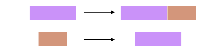
Figure 2. The two Fibonacci prototiles $\alpha$, $\beta$ (left) together with their inflations (right).

Figure 3. A Fibonacci tiling.

Example 2.18.

Let $\tau=\frac{1+\sqrt{5}}{2}$ be the golden ratio.

The Fibonacci inflation system is defined as follows: see Figure 2 for an Illustration.

• There are two prototiles $\alpha,\beta$, which are intervals of length $\tau$ and $1$ respectively, centered at $0$.

• The scaling constant is $\tau$

• $\varrho_{\alpha}$ is given by concatenating $\alpha$ and $\beta$ to cover an interval of length $\tau^{2}$

• $\varrho_{\beta}$ is given by a single $\alpha$.

See Figure 3 for an example of a Fibonacci tiling. Clearly Fibonacci tilings are FLC, as, for every $R>0$, there are only finitely many ways to cover $B_{R}$ with non-overlapping intervals of length $1$ and $\tau$, up to translation.

Its inflation matrix is $A=\begin{pmatrix}1&1\\ 1&0\end{pmatrix}$. One can check that $A^{2}$ is strictly positive, so this system is primitive. As $\tau$ is irrational, Fibonacci tilings are necessarily aperiodic.

Figure 4. The two kinds of prototiles for the Penrose inflation system, along with their corresponding inflations. Note that isometries may flip the orientation of the tiles: we display ”flipped” tiles in a darker color to distinguish them. If a tile is rotated or reflected, its inflation is transformed in the same way.

Figure 5. The Penrose tiling by half-kites and half-darts. In this article we will prove this tiling is hyperuniform and number rigid.

Example 2.19.

We define the Penrose inflation system as follows:

• The prototiles are two triangles, which we call half-kites and half-darts (see Figure 4), as well as their rotations by multiples of $\frac{2\pi}{10}$ and reflections.

• The scaling constant is $\tau$

• The inflation $\varrho$ is defined as in Figure 4.

See Figure 5 for an example of a Penrose tiling.

One can check that the inflation rule is primitive and FLC. Furthermore, Penrose tilings are aperiodic and every tile appears in finitely many orientations.

Its (reduced) inflation matrix is $A_{\text{red}}=\begin{pmatrix}2&1\\ 1&1\end{pmatrix}$, whose eigenvalues are $\tau^{2},-\tau^{-2}$.

Alternatively, one could define the Penrose system using only translations, using Lemma 2.17: this would be an inflation system with $40$ prototiles, corresponding to all the valid rotations and reflections of the half-kite and half-dart. Therefore, the corresponding full inflation matrix has dimension $40\times 40$.

Figure 6. The inflation rule for Ammann-Beenker tilings: the scaling constant is the silver mean $\lambda=1+\sqrt{2}$. As in the Penrose case, reflected triangles are drawn in different colors: for rhombi this is not necessary because their inflation is reflection-invariant.

Figure 7. An Ammann-Beenker tiling.

Example 2.20.

We define the A5 Ammann-Beenker inflation system as follows: it has scaling constant $\lambda=1+\sqrt{2}$ and prototiles and inflation rule as in Figure 6.

This is primitive and FLC, and the corresponding inflation tilings are always aperiodic.

Its reduced inflation matrix is given by $A_{\text{red}}=\begin{pmatrix}3&2\\ 4&3\end{pmatrix}$.

Example 2.21.

Recently, Smith, Myers, Kaplan, and Goodman-Strauss [27] discovered the existence of “einsteins”: that is, single tiles which can only tile the plane aperiodically. The most famous example has been christened “the hat”, and the corresponding tilings are called hat tilings or Smith tilings.

Hat tilings can be obtained from so-called HPTF tilings, involving four different tiles (called “metatiles”), which have a combinatorial substitution rule [26]. This is not an inflation rule, as the displacements of the tiles for each step do not stay the same for different levels: one can build up supertiles by adjoining tiles in a well defined way, . However, one can slightly change the shape of one tile to obtain an inflation system, which Baake, Gähler, and Sadun [8] call the CAP rule: the corresponding tilings are combinatorially equivalent to the HPTF tilings (see [26, Figure 2.8]). This is still not a stone inflation, but one can make it into a stone inflation by using fractal tiles as in [8, Figure 3].

3. Point processes

3.1. Point processes in $G$

Many important concepts we will be interested in, such as hyperuniformity, number rigidity and diffraction, are best described in terms of point processes. Here we will recall the basic concepts we need. We are mostly following the approach and notation from Björklund and Hartnick [9], except that we act from the left instead of from the right.

In this subsection, let $G$ be a (possibly nonabelian) locally compact, second countable, unimodular group. Let $m_{G}$ be its Haar measure.

Given some probability space $(\Omega,\mu)$ on which $G$ acts probability measure preservingly from the left, a random measure is a left $G$-equivariant measurable function

$$\Lambda:\Omega\to M(G)\qquad\omega\mapsto\Lambda_{\omega}$$

where $M(G)$ has its usual sigma algebra. We say $\Lambda$ is a point process if it is almost always positive and supported on a locally finite set, and a simple point process if $\Lambda$ also has measure $1$ at each atom. If $\Lambda$ is simple we can identify each measure with its support, which is a locally finite set.

From now on, we will assume every random measure is locally square integrable: that is, for all $B\subset G$ with $m_{G}(B)<\infty$, we have $\mathbb{E}[\Lambda(B)^{2}]<\infty$. We will also assume every random measure is stationary: that is, $g\Lambda$ has the same distribution as $\Lambda$ for all $g\in G$.

Example 3.1.

Let $\Gamma$ be a lattice in $G$. Then the space of cosets $G/\Gamma$ can be given a $G$-invariant probability measure, so we get a point process $\Lambda_{\Gamma}$ by sending

$$g\Gamma\mapsto\sum_{h\in g\Gamma}\delta_{h}$$

Example 3.2 ([22]).

Let $\lambda>0$. Then the Poisson process with intensity $\lambda$ is the unique point process $\Lambda_{\text{Poiss}}$ such that

• for all disjoint $B_{1},B_{2}\subset G$, $\Lambda_{\text{Poiss}}(B_{1})$ and $\Lambda_{\text{Poiss}}(B_{2})$ are independent random variables, and

• For all $B\subset G$, $\mathbb{E}[\Lambda_{\text{Poiss}}(B)]=\lambda m_{G}(B)$

For us, the most important examples of point processes will be the ones coming from inflation systems.

Example 3.3.

Let $\mathcal{S}$ be an inflation system, which is primitive and FLC. Then the space of inflation tilings $\Omega_{\mathcal{S}}$ is uniquely ergodic (see Remark 2.13), so we can define a point process $\Omega_{\mathcal{S}}$ on $\mathbb{R}^{d}\rtimes O(d)$ by

$$T\mapsto\sum_{gt\in T}\delta_{g}$$

Intuitively, $\Lambda_{\mathcal{S}}(B)$ counts how many tiles in $T$ have their center in the set $B$, where $B\subset\mathbb{R}^{d}\rtimes O(d)$ and $T$ is a random element of $T\in\Omega_{\mathcal{S}}$. If $T$ is a linearly repetitive FLC tiling, we can define a point process $\Lambda_{T}$ in the same way: if $T$ is an inflation tiling, $\Lambda_{T}$ and $\Lambda_{\mathcal{S}}$ are equally distributed.

For stationary point processes, the first and second moments are characterized by the intensity and autocorrelation of the point process.

Definition 3.4.

The intensity of $\Lambda$ is the unique $\iota(\Lambda)\in\mathbb{R}$ such that

$$\mathbb{E}[\Lambda(f)]=\iota(\Lambda)m_{G}(f)$$

for all $f\in\mathcal{L}_{c}^{\infty}(G)$.

Definition 3.5.

The autocorrelation measure $\eta$ of $\Lambda$ is the unique measure on $G$ such that

$$\eta(\check{f}_{1}*f_{2})=\mathbb{E}[\Lambda(f_{1}){\Lambda(f_{2})}]$$

for all $f_{1},f_{2}\in\mathcal{L}_{c}^{\infty}(G)$.

Remark 3.6.

Let $\mu$ be a random measure. Then its $n$-th moment is the unique measure on $G^{n}$ such that, for all Borel $B_{1},\cdots,B_{n}\subset G$, we have

$$M_{\mu}^{n}(B_{1}\times\cdots\times B_{n})=\mathbb{E}[\mu(B_{1})\cdots\mu(B_{n})]$$

assuming it exists. Under the assumption that $\mu$ is stationary, $M^{n}_{\mu}$ is also left-$G$-invariant measure. Using the projection $\pi:G^{n}\to G^{n-1}$ given by $(g_{1},\cdots,g_{n})\mapsto(g_{1}^{-1}g_{2},\cdots,g_{n})$ one can write $M^{n}_{\mu}$ in terms of a measure in $G^{n-1}$: in particular, the first and second moments are given by $M^{1}_{\mu}(f)=i(\mu)m_{G}(f)$ and $M^{2}_{\mu}(f_{1}\otimes f_{2})=\eta_{\mu}(\check{f}_{1}\otimes f_{2})$ respectively.

Example 3.7.

Let $\Gamma\subset G$ be a lattice, with Borel fundamental domain $F$. Then $\iota(\Lambda_{\Gamma})=m_{G}(F)^{-1}$: this quantity is often called the covolume of $\Gamma$. Its autocorrelation is given by $\eta=\iota(\Lambda_{\Gamma})^{2}\delta_{\Gamma}$, where $\delta_{\Gamma}=\sum_{g\in\Gamma}\delta_{g}$.

The Poisson process $\Lambda_{\text{Poiss}}$ with intensity $\lambda$ has autocorrelation $\eta=\lambda^{2}m_{G}+\lambda\delta_{e}$.

Now assume $G=\mathbb{R}^{d}$. The autocorrelation measure is positive and positive definite. Therefore, the following definition makes sense:

Definition 3.8.

The diffraction of $\Lambda$ is the Fourier transform $\hat{\eta}\in M(\mathbb{R}^{d})$ of its autocorrelation measure.

The diffraction measures of $\Lambda_{\Gamma}$ and $\Lambda_{\text{Poiss}}$ are $\hat{\eta}=\iota(\Lambda_{\Gamma})^{-2}\delta_{\Gamma^{*}}$(by Poisson summation) and $\hat{\eta}=\lambda^{-2}\delta_{e}+\lambda^{-1}m_{\mathbb{R}^{d}}$, respectively. Here $\Gamma^{*}$ is the dual lattice to $\Gamma$.

Remark 3.9.

Let $\Gamma\subset\mathbb{R}^{d}$ be an FLC, linearly repetitive set. Then its autocorrelation of its point process is pure point and given by

$$\gamma_{\Gamma}(z)=\lim_{R\to\infty}\frac{\#\{x\in B_{r}\mid x-z\in\Gamma\}}{\operatorname{Vol}(B_{r})}$$

In the literature of aperiodic order, one usually one defines the autocorrelation of a set of points using a formula like the above, instead of our definition coming from point process theory: one can also define a formula like this in the nonabelian case. This is an important consequence of unique ergodicity, as it means that properties of the point process translate to properties of individual tilings. However, for us, the point process approach will be more convenient, so we will not pursue this further. See Baake and Grimm [4, Chapter 9] for a more detailed explanation of the ergodic approach to autocorrelation and diffraction.

3.2. Powder diffraction

So far, we have defined diffraction for point processes over the group $G=\mathbb{R}^{d}$. In this subsection, we introduce powder diffraction, which gives us a concept of diffraction for the group $G={\mathbb{R}^{d}\rtimes O(d)}$. Powder diffraction can be defined by averaging over the action of $K=O(d)$ and reducing to the abelian case. Powder diffraction has already been considered for certain aperiodic tilings, such as pinwheel tilings: see Baake, Frettlöh, and Grimm [6] for more details.

Our approach can be understood as a special case of spherical diffraction, which can be applied in the wide generality of Gelfand pairs: see van Dijk [34, Chapter 6, Chapter 7.1] for an exposition of this general framework and how ${\mathbb{R}^{d}\rtimes O(d)}$ fits into it. While we do not assume familiarity with this theory, and the properties we need can be proved from classical Fourier theory by elementary means, this does help justify powder diffraction as a useful notion and hints at directions for further research.

In this subsection, let $G=\mathbb{R}^{d}\rtimes O(d)$ and $K=O(d)$. Let $m_{K}$ be a Haar probability measure on $K$.

If $f$ is an integrable function on $G$, we define $f_{K}\in L^{1}(\mathbb{R}^{d})$ by $f_{K}(x)=\int_{K}f(gk)dm_{K}(k)$. If $f$ is an integrable function on $\mathbb{R}^{d}$, we define $\prescript{}{K}{f}\in L^{1}(\operatorname{{[0,\infty)}})$ by $\prescript{}{K}{f}(r)=\int_{K}f(k(rv))dm_{K}(k)$, where $v\in\mathbb{R}^{d}$ is any vector of length $1$. If $\mu$ is a measure on $G$ or $\mathbb{R}^{d}$, we define $\mu_{K}\in M(\mathbb{R}^{d})$ and $\prescript{}{K}{\mu}\in M(\operatorname{{[0,\infty)}})$ analogously.

Averaging over $K$, we can now define the radial Fourier transform for functions.

Definition 3.10.

Let $f\in L^{1}(G)$. We define its radial Fourier transform $\hat{f}\in L^{1}(\operatorname{{[0,\infty)}})$ by $\hat{f}=\prescript{}{K}{(\widehat{f_{K}})}$, where $\widehat{f_{K}}$ is the Fourier transform of $f_{K}\in L^{1}(\mathbb{R}^{d})$.

Definition 3.11.

Let $\mu\in M(G)$ be such that $\mu_{K}$ is a Fourier transformable measure on $\mathbb{R}^{d}$. We define the radial Fourier transform $\hat{\mu}$ by $\hat{\mu}=\prescript{}{K}{(\widehat{\mu_{K}})}$.

The radial Fourier transform for functions can be given by an explicit formula, related to the well-known Hankel transform. For general $d$, this formula is best given in terms of the following function, which we call spherical functions (not to be confused with spherical harmonics, which are certain functions on $S^{2}$ important in harmonic analysis).

Definition 3.12.

For $r>0$, the $d$-dimensional spherical function $\sigma$ is an analytic function on $\operatorname{{[0,\infty)}}$ given by

$$\sigma(k)=\int_{S^{d}}e^{-2\pi ikx_{1}}dm_{S^{d}}(x)$$

Lemma 3.13.

Let $\varphi\in L^{1}(G)$. Then its radial Fourier transform is given by

$$\hat{\varphi}(r)=\int_{0}^{\infty}\prescript{}{K}{\varphi}_{K}(s)\sigma(rs)s^{d-1}ds$$

for $r\in[0,\infty)$

Remark 3.14.

By classical results about Bessel functions, the $d$-dimensional spherical functions are given by

$$\sigma(k)=\Gamma(\frac{d}{2})\frac{J_{\frac{d}{2}-1}(2\pi k)}{(2k)^{\frac{d}{2}-1}}$$

where $J_{\nu}$ is the Bessel function of the first kind and order $\nu$, and $\Gamma$ is the gamma function. Due to the properties of Bessel functions, $\sigma(0)=1$ and, if $d>1$, $\lim_{k\to\infty}\sigma(k)=0$.

We will mostly be interested in point processes where $d=2$, in which case the spherical function is given by $\sigma(k)=J_{0}(r)$.

Let $\Lambda$ be a point process on $G$, with autocorrelation $\eta$. Then $\eta_{K}$ is positive and positive definite, so the following definition makes sense.

Definition 3.15.

Let $\Lambda$ be a point process on $G$. Its powder diffraction is the measure $\theta\in M(\operatorname{{[0,\infty)}})$ defined by $\theta=\hat{\eta}$, where $\eta\in M(G)$ is the autocorrelation of $\Lambda$.

3.3. Hyperuniformity, rigidity and diffraction

Now let $\Lambda$ be a point process in $\mathbb{R}^{d}$. We are interested in the following properties:

Definition 3.16 (Torquato and Stillinger [33]).

We say $\Lambda$ is hyperuniform if

$$\lim_{R\to\infty}\frac{\operatorname{Var}(\Lambda(B_{R}))}{R^{d}}=0$$

For any $B\subset\mathbb{R}^{d}$, let $S(B)=\{\Lambda_{\omega}|_{B}|\omega\in\Omega\}$ be the set of measures one can get by restricting $\Lambda$ to $B$.

Definition 3.17 (Ghosh and Peres [19]).

We say $\Lambda$ is number rigid if the following holds: for every bounded $B\subset\mathbb{R}^{d}$ there exists a measurable function $\Phi:S(B^{c})\to\mathbb{N}$ such that $\#\Lambda\cap B=\Phi(\Lambda\cap B^{c})$ with probability $1$

Remark 3.18.

Let $T$ be an FLC, linearly repetitive tiling and $\Lambda_{T}$ the corresponding point process. Then we should imagine $\Lambda_{T}$ to be a “random translation” of $T$: in particular, for $r>0$, $\Lambda_{T}\cap B_{r}$ is a “random ball” in $T$. It would be possible to define hyperuniformity of $\Lambda_{T}$ in terms of $T$, using ergodic formulas.

It turns out that hyperuniformity and number rigidity can be determined using the diffraction measure.

Theorem 3.19.

• If

  $$\lim_{r\to 0}\frac{\hat{\eta}(B_{r}-\{0\})}{r^{d}}=0$$

  then $\Lambda$ is hyperuniform.

• If there exists some $\epsilon>0$ and a sequence $(r_{n})_{n\in\mathbb{N}}$ such that $r_{n}\to 0$ and

  $$\lim_{n\to 0}\frac{\hat{\eta}(B_{r_{n}}-\{0\})}{r_{n}^{2d+\epsilon}}$$

  then $\Lambda$ is number rigid.

The criterion for obtaining hyperuniformity was already known in some form to Torquato and Stillinger [33], in terms of the structure factor $S(k)$, and the criterion for number rigidity is due to Ghosh and Peres [19]. They do not prove this in the generality we need: in particular, Ghosh and Peres assume the point processes have absolutely continuous diffraction, which we do not assume. However, this assumption can be removed: Björklund and Hartnick [9] have proven the criteria for hyperuniformity and number rigidity in the general case.

One sees that it is, in general, interesting to know how fast $\hat{\eta}(B_{r}-\{0\})$ decays as $r\to 0$. It is helpful to boil this down to a single number.

Definition 3.20.

The (lower) degree of uniformity $\underline{h}(\Lambda)$ is the local dimension of $\hat{\eta}|_{B_{r}-\{0\}}$ at $0$. That is, we define:

$$\underline{h}(\Lambda)=\liminf_{r\to 0}\frac{\hat{\eta}(B_{r}-\{0\})}{\log r}$$

Then, by Theorem 3.19, $\underline{h}(\Lambda)>d$ implies $\Lambda$ is hyperuniform and $\underline{h}(\Lambda)>2d$ implies $\Lambda$ is number rigid, as we mentioned in Theorem 1.3 from the introduction.

Remark 3.21.

The criterion for number rigidity is sufficient, but not at all necessary: there exist point processes where $\hat{\eta}(B_{r}-\{0\})$ does not decay fast around zero and yet are number rigid. In fact, as pointed out by Klatt and Last [21], there exists point processes which are antihyperuniform but maximally rigid (and thus number rigid), such as the Poisson line intersection process.

Example 3.22.

Let $\Lambda_{\text{Poiss}}$ be the Poisson process with intensity $\lambda$. Then its diffraction is $\hat{\eta}=\lambda^{-2}\delta_{0}+\lambda^{-2}m_{G}$ Therefore, its diffraction satisfies $\hat{\eta}(B_{r}-\{0\})=\lambda^{-d}r^{d}$. This implies $\underline{h}(\Lambda_{\text{Poiss}})=d$.

Let $\Gamma\subset\mathbb{R}^{d}$ be a lattice. Then Poisson summation implies that the diffraction of its point process is $\hat{\eta}=\iota(\Lambda_{\Gamma})^{-2}\delta_{\Gamma^{*}}$, where $\Gamma^{*}$ is the lattice dual to $\Gamma$. If one removes the origin, $\hat{\eta}$ is zero in a ball around the origin, which implies $\underline{h}(\Lambda_{\Gamma})=\infty$, and Therefore, $\Lambda_{\Gamma}$ is both hyperuniform and number rigid.

Looking at both of these examples, one can understand $\underline{h}(\Lambda)$ as a measure of how “uniform” the point process is, hence we call a process where $\underline{h}(\Lambda)$ is higher than it would be for the Poisson process “hyperuniform”.

Now let $\Lambda$ be a point process on $G={\mathbb{R}^{d}\rtimes O(d)}$, with powder diffraction $\theta$. Then $\Lambda_{K}$ is a point process on $\mathbb{R}^{d}$, which we get by “forgetting” the orientations of the points in $\Lambda$: let $\hat{\eta}$ be the diffraction of $\Lambda_{K}$. By definition of the radial Fourier transform, we have $\hat{\eta}(B)=\theta(\prescript{}{K}{B})$ for all $O(d)$-invariant Borel $B\subset\mathbb{R}^{d}$. In particular, $\hat{\eta}(B_{r}-\{0\})={\theta}((0,r))$. If we define $\underline{h}(\Lambda)=\lim_{r\to 0}\frac{\log\theta((0,r))}{\log r}$, we get:

Theorem 3.23.

Let $\Lambda$ be a point process on ${\mathbb{R}^{d}\rtimes O(d)}$ with powder diffraction $\theta$. Then $\underline{h}(\Lambda)=\underline{h}(\Lambda_{K})$

Therefore, we can use powder diffraction estimate the decay of $\hat{\eta}$, and determine hyperuniformity and rigidity of $\Lambda_{K}$. We say $\Lambda$ is hyperuniform or number rigid if $\Lambda_{K}$ is.

Remark 3.24.

One could also define hyperuniformity and rigidity for point processes in ${\mathbb{R}^{d}\rtimes O(d)}$ by copying Definitions 3.16 and 3.17. For hyperuniformity this amounts to the same thing, but for rigidity this would lead to somewhat different concepts. We stick with our definition.

4. Colored point processes

4.1. Colored point processes

A simple point process, as we have seen, can be understood as a random discrete set of points in $G$. However, when dealing with tilings, it will be necessary to keep track of the different kinds of tiles that may occur. For this we will use the formalism of colored point processes.

Definition 4.1.

A colored point process $\boldsymbol{\Lambda}$ with $\ell$ colors is a vector $\boldsymbol{\Lambda}=(\Lambda_{1},\cdots,\Lambda_{\ell})$ of point processes with the same underlying probability space $(\Omega,\mu)$, whose atoms are $\mu$-almost always disjoint.

Similar to the uncolored case, we may understand $\boldsymbol{\Lambda}$ as a vector of random invariant point sets. A colored point set is a vector of point sets $\boldsymbol{\Gamma}=(\Gamma_{1},\cdots,\Gamma_{\ell})$.

Example 4.2.

Let $\mathcal{S}$ be a primitive, FLC inflation system. We can define a colored point process $\boldsymbol{\Lambda}$ on $\mathbb{R}^{d}\rtimes O(d)$ with probability space $\Omega_{\mathcal{S}}$ as follows: for $i\in[\ell]$, we define $\Lambda_{i}$ by

$$T\mapsto\sum_{gt_{i}\in T}\delta_{g}$$

That is, if $B$ is a Borel subset of $\mathbb{R}^{d}\rtimes O(d)$, then $\Lambda_{i}(B)$ counts how many tiles of color $i$ are in the set $B$.

If $T$ is an FLC, linearly repetitive tiling (not necessarily coming from an inflation) one can define a point process in the same way.

Given a colored point process $\boldsymbol{\Lambda}$, one can get many point processes from it: if $w\in\mathbb{R}^{\ell}$ is a positive vector, we define the weighing $w^{T}\boldsymbol{\Lambda}=\sum_{i=1}^{\ell}w_{i}\Lambda_{i}$. For example, the sum process $\Lambda=\sum_{i=1}^{\ell}\Lambda_{i}$ is a weighing of $\boldsymbol{\Lambda}$, but so are the individual components $\Lambda_{i}$, for example. If $\boldsymbol{\Lambda}$ is simple and the supports of the individual colors are disjoint, the sum process is the same as the process $\dot{\bigcup}_{i=1}^{\ell}\Lambda_{i}$, where we are identifying simple point processes on $G$ with their supports.

Definition 4.3.

Let $\boldsymbol{\Lambda}$ be a colored point process. We say $\boldsymbol{\Lambda}$ is hyperuniform (resp. number rigid) if all its weighings are hyperuniform (resp. number rigid).

If $T$ is a suitable linearly repetitive FLC tiling, we say $T$ is hyperuniform or number rigid if the associated colored point process $\boldsymbol{\Lambda}_{T}$ (as in Example 4.2) is.

Let $\boldsymbol{\Lambda}$ be a colored point process. We assume $\boldsymbol{\Lambda}$ is locally square integrable, meaning that all of its components are locally square integrable point processes. As in the non-colored case, we will be interested in the moments of a colored point process.

Definition 4.4.

The intensity vector $\boldsymbol{\iota}(\boldsymbol{\Lambda})=(\iota_{i}{(\boldsymbol{\Lambda})})_{i=1}^{\ell}\in\mathbb{R}^{\ell}$ of $\boldsymbol{\Lambda}$ is the unique vector such that such that

$$\mathbb{E}[{\Lambda}_{i}(f)]=\iota({\Lambda}_{i})m_{G}(f)$$

for all $f\in\mathcal{L}_{c}^{\infty}$, $i\in[\ell]$

Definition 4.5.

The autocorrelation matrix $\boldsymbol{\eta}=(\eta_{ij})_{i,j=1}^{\ell}$ of $\boldsymbol{\Lambda}$ is the unique $\ell\times\ell$ matrix of measures on $G$ such that

$${\eta}_{ij}(\check{f}_{1}*f_{2})=\mathbb{E}[{\Lambda}_{i}(f_{1}){{\Lambda}_{j}(f_{2})]}]$$

for all $f_{1},f_{2}\in\mathcal{L}_{c}^{\infty}(G)$, $i,j\in[\ell]$

The intensity and autocorrelation of $w^{T}\boldsymbol{\Lambda}$ are given by $w^{T}\boldsymbol{\iota}(\boldsymbol{\Lambda})$ and $w^{T}\boldsymbol{\eta}_{\boldsymbol{\Lambda}}w$, respectively. In particular, $\iota(\Lambda)$ is the intensity of the sum point process $\Lambda$, we have $\iota(\Lambda)=\sum_{i=1}^{\ell}{\iota}_{i}(\boldsymbol{\Lambda})$. If $\eta$ is the autocorrelation of the sum point process $\Lambda$, we have $\eta=\sum_{i,j=1}^{\ell}{\eta}_{ij}$.

4.2. Powder diffraction of colored point processes

Now let $G=\mathbb{R}^{d}\rtimes O(d)$ and $K=O(d)$. Let $\boldsymbol{\Lambda}$ be a colored point process in $G$ with autocorrelation matrix $\boldsymbol{\eta}$.

Theorem 4.6.

For any $m,n\in[\ell]$, the coefficients ${\eta}_{mn}$ of the autocorrelation matrix are radially Fourier transformable. The corresponding transforms $\theta_{mn}=\hat{\eta}_{mn}$ fulfill $\theta_{nm}=\overline{\theta_{mn}}$.

Proof.

For any $m$, we have ${\eta}_{mm}(f^{*}*f)=\mathbb{E}[\overline{{\Lambda}_{m}(f)}{\Lambda}_{m}(f)]$ for all $f\in\mathcal{L}_{c}^{\infty}(G)$, which makes ${\eta}_{mm}$ positive definite. Therefore, its radial Fourier transform exists and is positive.

For $m\neq n$, we use the following polarization identity (compare with [7, Theorem 3.23]):

$${\eta}_{mn}(f^{*}*f)=\mathbb{E}[{\overline{\Lambda_{m}(f)}}{{\Lambda}_{n}(f)}]=\frac{1}{4}\sum_{l=1}^{4}i^{l}\mathbb{E}[({\overline{\Lambda_{m}(f)+i^{l}{\Lambda}_{n}(f))}}{({\Lambda}_{m}(f)+i^{l}{\Lambda}_{n}(f))}]$$

Each of the individual summands is positive definite and therefore radial Fourier transformable, which means $\theta_{mn}$ also is (the resulting radial Fourier transform may be complex-valued). The conjugation symmetry can be seen from the polarization identity ∎

We call the matrix of measures $\boldsymbol{\theta}=(\theta_{mn})_{m,n=1}^{\ell}\in M(\operatorname{{[0,\infty)}})^{\ell\times\ell}$ the powder diffraction matrix of $\boldsymbol{\Lambda}$, and we define the lower degree of uniformity of $\boldsymbol{\Lambda}$

$$\underline{h}(\boldsymbol{\Lambda})=\lim_{r\to 0}\frac{\lVert\boldsymbol{\theta}\rVert((0,r))}{\log r}$$

If $w^{T}\boldsymbol{\Lambda}$ is a weighing of $\boldsymbol{\Lambda}$ with powder diffraction $\theta$, we have

$$\theta=w^{T}\boldsymbol{\theta}=w\sum_{i,j=1}^{\ell}w_{m}w_{n}\theta_{mn}$$

Therefore, we get $\underline{h}(\boldsymbol{\Lambda})\leq\underline{h}(w^{T}\boldsymbol{\Lambda})=\underline{h}((w^{T}\boldsymbol{\Lambda})_{K})$. This implies, as already mentioned in the introduction:

Proposition 4.7.

Let $\boldsymbol{\Lambda}$ be a colored point process.

• If $\underline{h}(\boldsymbol{\Lambda})>d$, $\boldsymbol{\Lambda}$ is hyperuniform (that is, all its weighings are hyperuniform).

• If $\underline{h}(\boldsymbol{\Lambda})>2d$, $\boldsymbol{\Lambda}$ is number rigid.

4.3. Point processes under convolution

In this section, we introduce a way to transform point processes which interacts well with autocorrelation and diffraction.

Let $G={\mathbb{R}^{d}\rtimes O(d)}$. If $\mu$ is a finite measure and $V$ is a translation bounded measure or function, we define $R_{\mu}V=V*\check{\mu}$ and $L_{\mu}V=\mu*V$. If $\boldsymbol{\mu}=(\mu_{ij})\in M(G)^{m\times n}$ is a matrix of finite measures and $\boldsymbol{V}=(V_{1},\cdots,V_{n})$ is a vector of measures or functions, we define $R_{\boldsymbol{\mu}}\boldsymbol{V}$ by $(R_{\boldsymbol{\mu}}\boldsymbol{V})_{i}=\sum_{j=1}^{n}R_{\mu_{ij}}V_{j}$, and $L_{\boldsymbol{\mu}}\boldsymbol{V}$ analogously. If $\boldsymbol{M}$ is a matrix of tile shift measures, we can also define $R_{\boldsymbol{\mu}}\boldsymbol{M}$ and $L_{\boldsymbol{\mu}}\boldsymbol{M}$, assuming the dimensions match.

A tile shift measure on $G$ is a positive measure supported on a finite set. If $\boldsymbol{\mu}$ is a matrix of tile shift measures, $R_{\boldsymbol{\mu}}$ and $L_{\boldsymbol{\mu}}$ send pure point measures to pure point measures, as we are taking a linear combination of translated copies of the original. Therefore, if $\boldsymbol{\Lambda}$ is a point process, $R_{\boldsymbol{\mu}}\boldsymbol{\Lambda}$ also is. In this case we say $R_{\boldsymbol{\mu}}\boldsymbol{\Lambda}$ is a tile shift of $\boldsymbol{\Lambda}$

Example 4.8.

In Example 2.19, we defined Penrose tilings in terms of certain tiles called half-kites and half-darts. Every half-kite and half-dart in a Penrose tiling is adjacent to another half-kite or half-dart with the opposite orientation. By joining every tile with its mirror image one gets a tiling by “kites” and “darts”: often, Penrose tilings are defined in terms of kites and darts instead of half-kites and half darts. If $T$ is a Penrose tiling by kites and darts and $T^{\prime}$ is the corresponding Penrose tiling by half-kites and half-darts, the associated point process $\boldsymbol{\Lambda}_{T^{\prime}}$ is a tile shift of $\boldsymbol{\Lambda}_{T}$.

Example 4.9.

In this article, we have chosen to represent tilings as sets of points by effectively placing a “center” in each prototile, which is convenient for us because it gives a clear correspondence between the points and the tiles. Another popular choice to turn a tiling into a set of points is using the set of vertices. If $T$ is a tiling such that the vertices and edges of neighboring tiles coincide, $\boldsymbol{\Gamma}$ is the associated vector of point sets given by the centers, and $V$ the set of vertices, $V$ is a tile shift of $\boldsymbol{\Gamma}$ (interpreted as pure point measures).

The reason tile shifts are a convenient concept for us is that they are compatible with intensity, autocorrelation and diffraction.

Theorem 4.10.

Let $\boldsymbol{\Lambda}$ be a colored point process with $\ell$ colors and $\boldsymbol{\mu}\in M(G)^{k\times\ell}$ a matrix of tile shift measures. Let $A$ be the matrix given by $A_{ij}=\mu_{ij}(G)$. Then we get the following formulas for the intensity, autocorrelation and powder diffraction of the point process $R_{\boldsymbol{\mu}}\boldsymbol{\Lambda}$:

1. $\boldsymbol{\iota}(R_{\boldsymbol{\mu}}\boldsymbol{\Lambda})=A\boldsymbol{\iota}(\boldsymbol{\Lambda})$

2. $\boldsymbol{\eta}_{R_{\boldsymbol{\mu}}\boldsymbol{\Lambda}}=L_{\boldsymbol{\mu}}\boldsymbol{\eta}_{\boldsymbol{\Lambda}}R_{\check{\boldsymbol{\mu}}}^{T}$

3. $\boldsymbol{\theta}_{R_{\boldsymbol{\mu}}\boldsymbol{\Lambda}}=\hat{\boldsymbol{\mu}}\boldsymbol{\theta}\hat{\boldsymbol{\mu}}^{T}$

Proof.

1. Let $f$ be a Borel function with $m_{G}(f)=1$. Then, for all $i\in[m]$ we have ${\iota}_{i}(R_{\boldsymbol{\mu}}\boldsymbol{\Lambda})=\sum_{j=1}^{\ell}\mathbb{E}[R_{\mu_{ij}}\Lambda_{j}(f)]=\sum_{j=1}^{\ell}\mathbb{E}[\Lambda_{j}(R_{\check{\mu}_{ij}}f)]=\sum_{j=1}^{\ell}\iota_{j}(\boldsymbol{\Lambda})m_{G}(R_{\check{\mu}_{ij}}f)$. By definition of $R_{\mu}$ we have $m_{G}(R_{\check{\mu}_{ij}}f)=a_{ij}m_{G}(f)=a_{ij}$, from which the theorem follows.

2. Let $\boldsymbol{\eta}=((\eta)_{ij})_{i,j=1}^{\ell}$ and $\boldsymbol{\eta}^{\prime}=(\eta_{ij}^{\prime})_{i,j=1}^{k}$ be the autocorrelation matrices of $\boldsymbol{\Lambda}$ and $R_{\boldsymbol{\mu}}\boldsymbol{\Lambda}$ respectively. Let $f_{1},f_{2}\in\mathcal{L}_{c}^{\infty}(G)$ and $(\rho_{n})_{n\in\mathbb{N}}$ be a sequence of approximate identities. Then we have

   $$\eta^{\prime}_{mn}(\check{f}_{1}*f_{2})=\sum_{i,j=1}^{\ell}\mathbb{E}[R_{\mu_{mi}}\Lambda_{i}(f_{1}){R_{\mu_{nj}}\Lambda_{j}(f_{2})}]=\sum_{i,j=1}^{\ell}\eta_{ij}(L_{\check{\mu}_{mi}}\check{f}_{1}*(R_{\check{\mu}_{nj}}f_{2}))=\sum_{i,j=1}^{\ell}\eta_{ij}(L_{\check{\mu}_{mi}}(\check{f}_{1}*f_{2})R_{{\mu}_{nj}})$$

   By substituting a sequence of approximate identities for $f_{2}$ and by definition of $R_{\boldsymbol{\mu}}$ and $L_{\boldsymbol{\mu}}$, we get $\boldsymbol{\eta}^{\prime}(f)=R_{\boldsymbol{\mu}}\boldsymbol{\eta}(f)L_{\boldsymbol{\mu}}^{T}$ for all $f\in\mathcal{L}_{c}^{\infty}$.

3. As the components of $\boldsymbol{\mu}$ are finite and supported on a finite set, $\hat{\boldsymbol{\mu}}$ is a matrix of positive, analytic functions. The radial Fourier transform, as the classical Fourier transform, maps convolution to multiplication. Therefore, $(3)$ follows from $(2)$.

∎

It is often possible to modify a point process using tile shifts in a way that doesn’t change the degree of uniformity, or changes it in a predictable way.

Corollary 4.11.

Let $\boldsymbol{\Lambda}$ be a colored point process and $\boldsymbol{\mu}$ be a matrix of tile shift measures. Let $A=(\mu_{ij})_{i,j}$.

1. If $A$ is nonzero we have $\underline{h}(R_{\boldsymbol{\mu}}\boldsymbol{\Lambda})\leq\underline{h}(\boldsymbol{\Lambda})$.

2. If $A$ is square and invertible, $\underline{h}(R_{\boldsymbol{\mu}}\boldsymbol{\Lambda})=\underline{h}(\boldsymbol{\Lambda})$

3. If $A=w^{T}\in\mathbb{R}^{\ell}$ is a row vector with nonnegative entries, $\underline{h}(R_{\boldsymbol{\mu}}\boldsymbol{\Lambda})=\underline{h}(w^{T}\boldsymbol{\Lambda})$, where $w^{T}\boldsymbol{\Lambda}=\sum_{i=1}^{\ell}w_{i}\Lambda_{i}$.

Proof.

As the components of $\boldsymbol{\mu}$ are finite positive measures, the components of $\hat{\boldsymbol{\mu}}$ are positive, analytic functions, and one can show that $\hat{\boldsymbol{\mu}}(\{0\})=A$. Therefore, the powder diffraction $\boldsymbol{\theta}_{R_{\boldsymbol{\mu}}\boldsymbol{\Lambda}}$ is close to $A\boldsymbol{\theta}_{\boldsymbol{\Lambda}}A^{T}$ around the origin.

1. In general, this means one can bound $\lVert\boldsymbol{\theta}_{R_{\boldsymbol{\mu}}\boldsymbol{\Lambda}}((0,r))\rVert=O(\lVert\boldsymbol{\theta}_{\boldsymbol{\Lambda}}((0,r))\rVert)$ for $r\to 0$, which implies $\underline{h}(R_{\boldsymbol{\mu}}\boldsymbol{\Lambda})\leq\underline{h}(\boldsymbol{\Lambda})$.

2. If $A$ is invertible, $\hat{\boldsymbol{\mu}}$ is invertible around the origin, so we can conclude $\underline{h}(R_{\boldsymbol{\mu}}\boldsymbol{\Lambda})\leq\underline{h}(\boldsymbol{\Lambda})$ in the same way.

3. If $A=w^{T}$, we have $A\boldsymbol{\theta}_{\boldsymbol{\Lambda}}A^{T}=w^{T}\boldsymbol{\theta}_{\boldsymbol{\Lambda}}w=\boldsymbol{\theta}_{w^{T}\boldsymbol{\Lambda}}$

∎

From this, it follows that the two Penrose processes from Example 4.8 have the same degree of uniformity. Furthermore, if, $T$ is an FLC, linearly repetitive tiling and $V$ is its set of vertices, their degrees of uniformity satisfy $\underline{h}(T)\leq\underline{h}(V)$, so if $T$ is hyperuniform or number rigid, $V$ also is.

Remark 4.12.

We have chosen to state the results of this section for $G={\mathbb{R}^{d}\rtimes O(d)}$, but most of the results of this section work for other groups: in particular, parts $(1)$ and $(2)$ of Theorem 4.10 work analogously for all locally compact, second countable groups $G$. If $G=\mathbb{R}^{d}$ one gets a version of $(3)$ using classical diffraction instead of powder diffraction.

5. Scaling of diffraction intensities near the origin

In the previous sections, we have seen that inflation tilings have many desirable properties. They are often aperiodic, FLC, repetitive and uniquely ergodic. However, none of these properties are unique to inflation tilings, and can be obtained by other methods, such as cut-and-project.

In this section, we will introduce renormalization relations, which are certain equations that follow from the self-similarity of inflation tilings. Using these relations, we will be able to prove the main theorem of this article, which gives a bound for the degree of uniformity of inflation tilings.

For all of this section, let $G={\mathbb{R}^{d}\rtimes O(d)}$, $K=O(d)$, and let $\mathcal{S}$ be a primitive, FLC inflation system with inflation matrix $A$ and inflation rule $\varrho$. Let $\boldsymbol{\Lambda}$ be the corresponding colored point process over $G$, with powder diffraction $\boldsymbol{\theta}$.

5.1. Renormalization

Recall that the map $\varrho:\Omega_{\mathcal{S}}\to\Omega_{\mathcal{S}}$ is defined by sending every tile $gt_{i}$ to a patch $(\lambda g)\varrho_{i}$. Let $\boldsymbol{\mu}_{\varrho}=(\mu_{i,j})_{i,j=1}^{\ell}$ be the matrix of tile shift measures given by $\mu_{ij}=\sum_{xt_{i}\in\varrho_{j}}\delta_{x}$. Write $R_{\varrho}=R_{\boldsymbol{\mu}_{\varrho}}$, $L_{\varrho}=L_{\boldsymbol{\mu}_{\varrho}}$, $R_{\check{\varrho}}=R_{\check{\boldsymbol{\mu}}_{\varrho}}$ and $L_{\check{\varrho}}=L_{\check{\boldsymbol{\mu}}_{\varrho}}$.

Theorem 5.1.

Let $\boldsymbol{\Lambda}$ be the colored point process associated to a primitive, FLC inflation system. Then $\boldsymbol{\Lambda}$ and $R_{\varrho}D_{\lambda}\boldsymbol{\Lambda}$ have the same distribution as point processes: in particular they have the same intensity, autocorrelation and diffraction.

Proof.

Let $\mu$ be the $G$-invariant probability measure on $\Omega_{\mathcal{S}}$ associated to $\boldsymbol{\Lambda}$. Let the measure $\varrho_{*}\mu$ be given by $\varrho_{*}\mu(B)=\mu(\varrho^{-1}(B))$. Then $\varrho_{*}\mu$ is also a $G$-invariant probability measure on $\Omega_{\mathcal{S}}$. As $\Omega_{\mathcal{S}}$ is a uniquely ergodic probability measure, we have $\varrho_{*}\mu=\mu$. By definition of the inflation map, $\varrho$ acts on the corresponding colored point process as follows: for all $T\in\Omega_{\mathcal{S}}$ and Borel $B\subset G$ we have $\boldsymbol{\Lambda}(\varrho(T),B)=R_{\varrho}D_{\lambda}\boldsymbol{\Lambda}(T,B)$. Therefore, $\boldsymbol{\Lambda}$ and $R_{\varrho}D_{\lambda}\boldsymbol{\Lambda}$ have the same distribution. ∎

From this, Theorem 4.10 gives us formulae for the intensity, autocorrelation, and diffraction of an inflation point process.

The renormalization formula for the intensity is well known: see for instance Baake and Grimm [4, Proposition 6.1]

Corollary 5.2.

$\boldsymbol{\iota}(\boldsymbol{\Lambda})$ satisfies the following relation

$$\boldsymbol{\iota}(\boldsymbol{\Lambda})=\lambda^{-d}A\boldsymbol{\iota}(\boldsymbol{\Lambda})$$

In other words, $\boldsymbol{\iota}(\boldsymbol{\Lambda})$ is a PF eigenvector of the inflation matrix $A$.

Baake, Grimm, Gähler and Mañibo [3, 7] already derived renormalization relations for the autocorrelation measure over $\mathbb{R}^{d}$. In our setting, Theorem 4.10 gives us a version that works over ${\mathbb{R}^{d}\rtimes O(d)}$. We do not need to assume $\varrho$ is injective.

Corollary 5.3 (Renormalization).

Let $\boldsymbol{\eta}_{\boldsymbol{\Lambda}}$ be the autocorrelation of $\boldsymbol{\Lambda}$. We get

$$\boldsymbol{\eta}_{\boldsymbol{\Lambda}}=L_{\varrho}(D_{\lambda}\boldsymbol{\eta}_{\boldsymbol{\Lambda}})R_{\check{\varrho}}^{T}$$

From this, we get the following renormalization relation for the diffraction. Recall that $\widehat{\boldsymbol{\mu}}_{\varrho}$ is the matrix valued analytic function on $\operatorname{{[0,\infty)}}$ given by taking the componentwise radial Fourier transform of $\boldsymbol{\mu}_{\varrho}$. By definition of $\boldsymbol{\mu}_{\varrho}$, we have $(\widehat{\boldsymbol{\mu}}_{\varrho})_{ij}=\sum_{xt_{i}\in\varrho_{j}}\sigma(\lvert x\rvert r)$, where $\sigma$ is the spherical function in dimension $d$ as in Definition 3.12.

Corollary 5.4.

The powder diffraction $\boldsymbol{\theta}$ satisfies

$$\boldsymbol{\theta}=\lambda^{-2d}\widehat{\boldsymbol{\mu}}_{\varrho}(D_{\lambda^{-1}}\boldsymbol{\theta})\widehat{\boldsymbol{\mu}}_{\varrho}^{T}$$

For this formula to tell us something useful about $\boldsymbol{\theta}$, we need some way to relate $D_{\lambda^{-1}}\boldsymbol{\theta}$ to $\boldsymbol{\theta}$. We will assume $\boldsymbol{\theta}$ is pure point: in this case we will write $\boldsymbol{\theta}(r)=\boldsymbol{\theta}(\{r\})$. Then Corollary 5.4 can be put in the following form:

Corollary 5.5.

Assume $\boldsymbol{\theta}$ is pure point, and let $\tilde{A}$ be the analytic matrix function given by $\tilde{A}(r)=\lambda^{-d}\widehat{\boldsymbol{\mu}}_{\varrho}(\lambda r)$. Then

$$\boldsymbol{\theta}(r)=\tilde{A}(r)\boldsymbol{\theta}(\lambda r)\tilde{A}(r)^{T}$$

Proof.

Let $r\in\operatorname{{[0,\infty)}}$, and choose a sequence $(f_{n})\in C_{c}(\operatorname{{[0,\infty)}})$ with the following properties:

• $f_{n}$ is supported in $B(r,\frac{1}{n})$

• $f_{n}(s)$ is monotonically decreasing as a function of $n$ for all $s\in\operatorname{{[0,\infty)}}$

• $f_{n}(r)=1$ for all $n$.

In particular, $f_{n}(s)$ converges pointwise to $1$ for $s=r$ and to $0$ otherwise. From the dominated convergence theorem, we get $\boldsymbol{\theta}(f_{n})\to\boldsymbol{\theta}(r)$ and $D_{\lambda^{-1}}\boldsymbol{\theta}(f_{n})\to\boldsymbol{\theta}(\lambda r)$. Then our claim follows using Corollary 5.4. ∎

Remark 5.6.

If $\boldsymbol{\theta}$ is not pure point, Corollary 5.4 applies to its pure point, absolutely continuous and singular continuous parts separately. Therefore, Corollary 5.5 still applies to the pure point part. It is possible to write a similar formula for the Lebesgue density of the absolutely continuous part (see [7]), but for the singular part we can not do this in general, as there is no similar concept of density available

It is easier to use the renormalization relation after the following dimensionality reduction trick.

Lemma 5.7.

If $\boldsymbol{\theta}$ is pure point, there exist vector-valued functions $\boldsymbol{v}_{1},\cdots,\boldsymbol{v}_{d}$ with the following property: for all $0<r\leq 1$, we have:

$$\boldsymbol{\theta}(r)=\sum_{i=1}^{d}\boldsymbol{v}_{i}(r)\boldsymbol{v}_{i}^{\dagger}(r)$$

and

$$\boldsymbol{v}_{i}(z)=\tilde{A}(r)\boldsymbol{v}_{i}(\lambda z)$$

for all $i\in[\ell]$

Proof.

For all $r$, $\boldsymbol{\theta}(r)$ is a Hermitian and positive semi-definite matrix, so there exists some a decomposition $\boldsymbol{\theta}(r)=\sum_{i=1}^{d}\boldsymbol{v}_{i}(r)\boldsymbol{v}_{i}^{\dagger}(r)$ for all $r$ individually, but these decompositions are not unique. Choose any such decomposition for all $\lambda^{-1}<|z|\leq 1$. Then we can define $\boldsymbol{v}_{i}$ in the whole punctured ball by $\boldsymbol{v}_{i}(z):=\tilde{A}(z)\boldsymbol{v}_{i}(\lambda z)$ recursively. ∎

5.2. Proof of the main theorem

The main result of this paper is the following theorem, which we already stated in the introduction:

Theorem 1.10.

Let $\mathcal{S}$ be an FLC, primitive inflation system, in dimension $d$ with at least two prototiles ($\ell\geq 2$). Let $\lambda$ be the scaling constant and $A_{\text{red}}$ the reduced inflation matrix. Assume $\mathcal{S}$ has pure point powder diffraction. Then the corresponding point process $\boldsymbol{\Lambda}$ satisfies

$$\underline{h}(\boldsymbol{\Lambda})\geq 2d-2\frac{\log\rho_{2}}{\log\lambda}$$

where $\rho_{2}$ is the absolute value of the second-largest eigenvalue of the reduced inflation matrix $A_{\text{red}}$.

This theorem works specially well if $A$ is small and has few eigenvalues, as we want the gap between the $PF$ eigenvalue $\lambda^{d}$ and the other eigenvalues to be as big as possible. A very important special case occurs whenever $A$ has irreducible characteristic polynomial.

Corollary 5.8.

Let $\mathcal{S}$ be an FLC, primitive inflation system with reduced inflation matrix $A$. Assume $\mathcal{S}$ has pure point powder diffraction, and $A$ has an irreducible characteristic polynomial. Then $\underline{h}(\boldsymbol{\Lambda})>2d$: in particular $\boldsymbol{\Lambda}$ is hyperuniform and number rigid.

Proof.

If the characteristic polynomial of $A$ is irreducible, the eigenvalues of $A$ are exactly the algebraic conjugates of $\lambda^{d}$, so $\rho_{2}$ is at most the largest absolute value of some algebraic conjugate of $\lambda^{d}$. As we are assuming $p$ has pure point diffraction, its pure point spectrum has values outside the origin. This implies $\lambda^{d}$ must be a Pisot number (see [30]), which means that $\rho_{2}<1$. Therefore, the formula from before implies $\underline{h}(\boldsymbol{\Lambda})\geq 2d-2\frac{\log(\rho_{2})}{\log(\lambda)}>2d$ ∎

For symbolic substitutions, the Pisot substitution conjecture states that, if the substitution is irreducible and Pisot, it must have discrete spectrum: see Akiyama, Barge, Berthé, Lee, and Siegel [1] for a survey of this conjecture. This has been proven for one-dimensional substitutions of two letters, and no counterexample is known. However, for inflation tilings in several dimensions, there is no agreement about what the Pisot conjecture should be, as irreducibility of the full inflation matrix is much rarer. We propose the following:

Conjecture 5.9.

Let $\mathcal{S}$ be an FLC, primitive inflation system (with at least two colors) with reduced inflation matrix $A$. Assume $A$ has an irreducible characteristic polynomial, and $\lambda^{d}$ is a Pisot number. Then $\mathcal{S}$ has pure point powder diffraction, and therefore, Theorem 1.10 applies.

For all of this section, let $\boldsymbol{\Lambda}$ be the point process coming from an inflation system $\mathcal{S}$ with inflation matrix $A$ and powder diffraction matrix $\boldsymbol{\theta}$. We assume this inflation system is primitive, FLC, and has pure point powder diffraction.

Our method to estimating hyperuniformity of these point processes is inspired by the approach of Baake and Grimm [5, Section 3.2-4] to hyperuniformity of certain one-dimensional inflation tilings: we use the renormalization relation to determine how the diffraction intensity along sequences of the form $\lambda^{-n}$. However, we give an elementary proof without using Lyapunov theory and without assuming an underlying cut and project structure.

Remark 5.10.

If $\boldsymbol{\Lambda}$ does not have pure point diffraction, the estimate of Theorem 1.10 still gives an upper bound for the decay of the pure point part of the diffraction around the origin, but the degree of hyperuniformity of $\boldsymbol{\Lambda}$ may be lower if the continuous part has slower decay.

We will prove Theorem 1.10 assuming $\ell>1$ first, in which case the inflation matrix $A$ does in fact have two distinct eigenvalues: we will handle the $\ell=1$ case in the end.

Recall that $\tilde{A}(r)=\lambda^{-d}\widehat{\boldsymbol{\mu}}_{\varrho}(\lambda r)$ and let $\tilde{A}=\lambda^{-d}A$, where $A$ is the inflation matrix of $\mathcal{S}$. $\tilde{A}$ is primitive and $\operatorname{Spec}(\tilde{A})=\lambda^{-d}\operatorname{Spec}(A)$: in particular the PF eigenvalue of $\tilde{A}$ is $1$. Let $\mu:=\frac{\rho_{2}}{\lambda^{d}}$: this is the absolute value of the second-largest eigenvalue of $\tilde{A}$. There exists some $C>0$ such that $\|\tilde{A}(r)-\tilde{A}\|\leq Cr$, and in particular $\tilde{A}(r)\to\tilde{A}$ as $r\to 0$. We also define $\tilde{A}^{(n)}(r)=\tilde{A}(\lambda^{-n+1}r)\tilde{A}(\lambda^{-n+2}r)\cdots\tilde{A}(r)$.

Recall that $\boldsymbol{\theta}(r)=\sum_{i}\boldsymbol{v}_{i}(r)\boldsymbol{v}_{i}(r)^{\dagger}$, with $\boldsymbol{v}_{i}(r)$ chosen as in Lemma 5.7. Then we have $\boldsymbol{v}_{i}(\lambda^{-n}r)=\tilde{A}^{(n)}(\lambda^{-1}r)\boldsymbol{v}_{i}(r)$ for all $r\leq 1$ and $i\in\{1,\cdots,\ell\}$.

For simplicity, we assume $A$ is diagonalizable by orthogonal vectors, which is true if $A$ is symmetric. Otherwise, one can choose a different scalar product such that the generalized eigenspaces become orthogonal, which yields an equivalent norm: one also needs to do slight adjustments if $A$ is not diagonalizable.

Let $v_{PF}$ be the nonnegative PF eigenvector of $\tilde{A}$, scaled such that $\lVert v_{PF}\rVert=1$. For $v\in\mathbb{R}^{q}$, let $v^{\parallel}=v_{PF}\langle v,v_{PF}\rangle$ and $v^{\bot}=v-v^{\parallel}$. If $v\neq 0$, define $q(v)=\frac{\lVert v^{\bot}\rVert}{\lVert v^{\parallel}\rVert}$ (if $v^{\parallel}=0$ we define $q(v)=\infty$).

Lemma 5.11.

For every $L>0$ one can choose $\epsilon>0$ with the following property: for all $r$ such that $r\leq\epsilon$ and all $v\in\mathbb{R}^{q}\setminus\{0\}$, we have either $q(v)>L$ or $\lim_{n\to\infty}q(\tilde{A}^{(n)}(r)v)=0$ exponentially fast.

Proof.

By definition of $q$, we have the following formulas for the parallel and orthogonal parts of a vector:

$$\lVert v^{\bot}\rVert=\sqrt{1+q(v)^{-2}}^{-1}\lVert v\rVert \lVert v^{\parallel}\rVert=\sqrt{1+q(v)^{2}}^{-1}\lVert v\rVert$$

From this we get the following formula

$$\lVert(\tilde{A}(r)v)^{\bot}\rVert=\lVert(\tilde{A}v)^{\bot}+((\tilde{A}(r)-\tilde{A})v)^{\bot}\rVert\leq(\mu\sqrt{1+q(v)^{-2}}^{-1}+Cr)\lVert v\rVert$$

And, similarly for the parallel part,

$$\lVert(\tilde{A}(r)v)^{\parallel}\rVert\geq(\sqrt{1+q(v)^{2}}^{-1}-Cr)\lVert v\rVert$$

Then, for all $r$ small enough, we get

$$q(\tilde{A}(r)v)\leq\frac{\mu\sqrt{1+q(v)^{-2}}^{-1}+Cr}{\sqrt{1+q(v)^{2}}^{-1}-Cr}=\frac{\mu q(v)+\sqrt{1+q(v)^{2}}Cr}{1-\sqrt{1+q(v)^{2}}Cr}\leq(\mu+2CLr)q(v)+2r$$

Therefore, by the Banach fixpoint theorem, we can find some bound $\epsilon>0$ such that, for all $v$ with $q(v)\geq L$ and all $r\leq\epsilon$, we have $\lim_{n\to\infty}q(A^{(n)}(r)v)=0$, and in fact it converges exponentially fast. ∎

Lemma 5.12.

For all $i\in[\ell]$, we have $\lim_{r\to 0}q(\boldsymbol{v}_{i}(r))=\infty$.

Proof.

Fix some $L\geq 0$: by Lemma 5.11, there is some $\epsilon>0$ such that, for all $r<\epsilon$, $q(\boldsymbol{v}_{i}(r))>L$ or $\lim_{n\to\infty}\boldsymbol{v}_{i}(\lambda^{-n}r)=0$. So we assume, towards a contradiction, that we have some $r_{0}<\epsilon$ such that $q(\boldsymbol{v}_{i}(r_{0}))\leq L$: as noted in the lemma, $\boldsymbol{v}(\lambda^{-n}r_{0})$ converges to $0$ exponentially fast as $r\to\infty$.

Then we have:

$$\lVert\tilde{A}(r)v\rVert\geq(\sqrt{1+q(v)^{2}}^{-1}-\mu\sqrt{1+q(v)^{-2}}^{-1}-Cr)\lVert v\rVert$$

assuming $z$ and $q(v)$ are small enough. Therefore, using the fact that $q(v_{i}(\lambda^{-n}r_{0}))\to 0$ exponentially fast, one can check that $n(\frac{\lVert\boldsymbol{v}_{i}(\lambda^{-n-1}r_{0})\rVert^{2}}{\lVert\boldsymbol{v}_{i}(\lambda^{-n}r_{0})\rVert^{2}}-1)\to 0$ as $n\to\infty$, which implies that $\sum_{n=0}^{\infty}\lVert\boldsymbol{v}_{i}(\lambda^{-n}r_{0})\rVert^{2}=\infty$ by Raabe’s series test.

On the other hand, let $\lVert\boldsymbol{\theta}\rVert_{F}$ be the pure point measure whose density at $r$ is the Frobenius norm of the matrix $\boldsymbol{\theta}$. This is a locally finite measure because all the $\theta_{ij}$ are locally finite. However, then we would have

$$\sum_{n=0}^{\infty}\lVert\boldsymbol{v}_{i}(\lambda^{-n}r_{0})\rVert^{2}\leq\lVert\boldsymbol{\theta}\rVert_{F}((0,r])<\infty$$

which is a contradiction. Therefore, we must have $q(\boldsymbol{v}_{i}(z_{0}))\geq L$ for all $z\in B_{\epsilon}^{\times}$. As we can find some such $\epsilon>0$ for every $L$, this proves the theorem. ∎

Proof of Theorem 1.10 for $\ell>1$.

Let $0<r<1$. Then we have

$$\boldsymbol{v}_{i}(\lambda^{-1}r)=\tilde{A}(r)\boldsymbol{v}_{i}(r)=(\tilde{A}(r)-\tilde{A})\boldsymbol{v}_{i}(r)+\tilde{A}\boldsymbol{v}_{i}^{\bot}(r)+\tilde{A}\boldsymbol{v}_{i}^{\parallel}(r)$$

We can estimate the three summands as follows

• $\lVert(\tilde{A}(r)-\tilde{A})\boldsymbol{v}_{i}(r)\rVert\leq\lVert\tilde{A}(r)-\tilde{A}\rVert\lVert\boldsymbol{v}_{i}(r)\rVert\leq Cr\lVert\boldsymbol{v}_{i}(r)\rVert$

• $\lVert\tilde{A}\boldsymbol{v}_{i}^{\bot}(r)\rVert\leq\mu\lVert\boldsymbol{v}_{i}(r)\rVert$

• $\lVert\tilde{A}\boldsymbol{v}_{i}^{\parallel}(r)\rVert\leq q(\boldsymbol{v}_{i}(r))^{-1}\lVert\boldsymbol{v}_{i}(r)\rVert$

Therefore,

$$\lVert\boldsymbol{v}_{i}(\lambda^{-1}r)\rVert\leq(\mu+Cr+q(\boldsymbol{v}_{i}(r))^{-1})\lVert\boldsymbol{v}_{i}(r)\rVert$$

Lemma 5.12 implies that $q(\boldsymbol{v}_{i}(r))$ goes to $\infty$ as $r\to 0$. Therefore, for all $r_{0}\leq 1$, we have $v(\lambda^{-n}r_{0})=O((\mu+\epsilon)^{n})$ for all $\epsilon>0$, where the implicit constant can be chosen to be independent of $r_{0}$ (but not necessarily $\epsilon$). It follows that $\lVert\boldsymbol{\theta}(\lambda^{-n}r_{0})\rVert=O((\mu+\epsilon)^{2n})$.

Then the radial distribution function $\theta((0,r))$ along the sequence $(\lambda^{-n})_{n}$ can be bounded as follows:

$$\lVert\boldsymbol{\theta}\rVert(0,r)=\sum_{r^{\prime}<\lambda^{-n}}\lVert\boldsymbol{\theta}\rVert(r^{\prime})=\sum_{\lambda^{-1}<r^{\prime}<1}\sum_{k=n}^{\infty}\lVert\boldsymbol{\theta}\rVert(\lambda^{-k}r^{\prime})=O((\mu+\epsilon)^{2n})$$

for all $\epsilon>0$, where in the last step we’re using the fact that $\lVert\boldsymbol{\theta}\rVert(\lambda^{-k}r^{\prime})$ decays like $(\mu+\epsilon)^{2k}$ and summing a geometric series.

Recall that $\mu=\frac{\varrho_{2}}{\lambda^{d}}$. From the aforementioned facts we can show

$$h(\boldsymbol{\Lambda})=\underline{\lim}_{r\to 0}\frac{\log\lVert\boldsymbol{\theta}\rVert((0,r))}{\log(r)}\geq\underline{\lim}_{k\to\infty}\frac{\log\lVert\boldsymbol{\theta}\rVert((0,\lambda^{-k}))}{\log(\lambda^{-k})}\geq\frac{\log(\mu^{2k})}{\log(\lambda^{-k})}=2d-2\frac{\log(\rho_{2})}{\log(\lambda)}$$

∎

Remark 5.13.

We are using the fact that, if $f:\operatorname{{[0,\infty)}}\to\operatorname{{[0,\infty)}}$ is a continuous function with $f(0)=0$, we have $\liminf_{r\to 0}\frac{\log f(r)}{\log(r)}\geq\liminf_{k\to\infty}\frac{\log(f(\lambda^{-k}))}{\log(\lambda^{-k})}$. This may not be true in general if we substitute $(\lambda^{-k})_{k\in\mathbb{N}}$ with some other sequence $(a_{k})_{k\in\mathbb{N}}$ tending to $0$. However, it does hold if $\frac{a_{k}}{a_{k+1}}$ is bounded.

5.3. Examples

Now we will apply Theorem 1.10 to several inflation systems and discuss the results.

Example 5.14.

Let $\mathcal{S}$ be the Fibonacci inflation system from Example 2.18. We have already discussed that it is primitive and FLC. It is also known that Fibonacci tilings can be obtained by cut-and-project methods. Therefore, we can apply Theorem 1.10.

Its inflation matrix is $A=\begin{pmatrix}1&1\\ 1&0\end{pmatrix}$, which implies $\rho_{2}=\tau^{-1}$. From this we get $\underline{h}(\boldsymbol{\Lambda})\geq 2-\frac{\log\tau}{\log\tau^{-1}}=4$. Therefore, Fibonacci tilings are hyperuniform and number rigid.

Example 5.15.

Let $\mathcal{S}$ be the Penrose inflation system from Example 2.19. Penrose tilings can be constructed by cut-and-project methods, so $\mathcal{S}$ fulfills of the conditions of Theorem 1.10.

Its reduced inflation matrix $A=\begin{pmatrix}2&1\\ 1&1\end{pmatrix}$ has irreducible characteristic polynomial, Therefore, Penrose tilings are hyperuniform and number rigid by Corollary 5.8. Specifically we get $\underline{h}(\boldsymbol{\Lambda})\geq 8$, which coincides with the calculations by Fuchs, Mosseri, and Vidal [15].

Alternatively, using Lemma 2.17, one could define a Penrose inflation system defined over $\mathbb{R}^{2}$. However, the full inflation matrix is $40\times 40$ and has $\rho_{2}=\tau$, which is not enough to prove either hyperuniformity or number rigidity. This illustrates how it really is advantageous to consider powder diffraction instead of classical diffraction.

By the same reasoning, the Ammann-Beenker tilings from Example 2.20 are hyperuniform and number rigid.

Example 5.16.

We can also apply Theorem 1.10 to systems from the Shield/Socolar family, as they are also cut-and-project. In particular, consider the partially decorated shield tiling from Baake and Grimm [4, Figure 6.16]. Here we have $\lambda=2+\sqrt{3}$ and $\rho_{2}=1$, which implies $\underline{h}(\boldsymbol{\Lambda}_{\text{shield}})\geq 4$. This is enough to conclude the corresponding shield tilings are hyperuniform, but may or may not be number rigid.

Example 5.17.

The ABCK inflation system is an inflation system on $\mathbb{R}^{3}$, with four prototiles (up to euclidean isometry): see Baake and Grimm [4, Section 6.7.1] for details on its construction. It is primitive and FLC, and it can be constructed via cut-and-project, so Theorem 1.10 is applicable. The reduced inflation matrix has eigenvalues $\tau^{3},\tau,-\tau^{-1},-\tau^{-3}$, Therefore, $\rho_{2}=\tau$ and $\underline{h}(\boldsymbol{\Lambda}_{\text{ABCK}})\geq 6-2=4$. This makes ABCK tilings hyperuniform, but we are not able to decide if they are rigid or not.

Example 5.18.

CAP inflation systems (see Example 2.21) can be given by a model set, so they have pure point diffraction. By Theorem 1.10 the associated point process $\boldsymbol{\Lambda}_{\text{CAP}}$ has $\underline{h}(\boldsymbol{\Lambda}_{\text{CAP}})\geq 4$, which implies hyperuniformity. Hat tilings can be obtained by decorating a deformation of CAP tilings. Unfortunately, the corresponding point process $\boldsymbol{\Lambda}_{\text{hat}}$ does not necessarily have $\underline{h}(\boldsymbol{\Lambda}_{\text{hat}})=\underline{h}(\boldsymbol{\Lambda}_{\text{CAP}})$, as the deformation from one to the other can not be given by a tile shift.

However, Baake, Gähler, and Sadun [8] have shown that they are topologically conjugate. Using the fact that the CAP inflation system forces the border, one can approximate hat tilings by tile shifts of CAP tilings, which implies hat tilings are also hyperuniform: see Appendix A for details.

Appendix A Deformations of inflation tilings

In this appendix, we will prove the following theorem about deformations of inflation tilings (we defer the relevant definitions to later in this section):

Theorem A.1.

Let $\boldsymbol{\Gamma}$ be the multiset of centers of an inflation tiling with inflation system $\mathcal{S}$ and $\boldsymbol{\Gamma}^{\prime}$ be a deformation of it (in the sense of Definition A.3). Assume $\mathcal{S}$ is primitive, FLC, defined over $\mathbb{R}^{d}$ and forces the border. Let $\boldsymbol{\Lambda}$ and $\boldsymbol{\Lambda}^{\prime}$ be the point processes associated to $\boldsymbol{\Gamma}$ and $\boldsymbol{\Gamma}^{\prime}$ respectively.

For all $0<k\leq 1$ we have: if $\underline{h}(\boldsymbol{\Lambda})>d+k$, then $\underline{h}(\boldsymbol{\Lambda}^{\prime})\geq d+k$

HPTF tilings are deformations of CAP tilings, and therefore:

Corollary A.2.

HPTF tilings and hat tilings are hyperuniform with $\underline{h}\geq 3$, as claimed in Example 5.18.

A.1. Deformation conjugacies

We will restrict ourselves to tilings $T$ defined over $\mathbb{R}^{d}$, for simplicity: then, unlike in the rest of its article, we consider the tiling space $\Omega_{T}:=\overline{T+\mathbb{R}^{d}}$ given as the closure of the orbit of $T$ under the group of translations $\mathbb{R}^{d}$, rather than the full group of isometries ${\mathbb{R}^{d}\rtimes O(d)}$.

For technical reasons, rather than working with tilings, we will want to work with Delone multisets. A Delone multiset, or colored Delone set, is a vector $\boldsymbol{\Gamma}=(\Gamma_{1},\cdots,\Gamma_{\ell})$ of Delone subsets of $\mathbb{R}^{d}$. Note that, if $T$ is a tiling with set of colored prototiles $\{t_{1},\cdots,t_{\ell}\}$, $T$ is uniquely determined by its Delone multiset $\boldsymbol{\Gamma}_{T}=(\Gamma_{1},\cdots,\Gamma_{\ell})$ given by $\Gamma_{i}=\{x|x+t_{i}\in T\}$, which we call its multiset of centers. However, a Delone multiset may or may not come from a tiling.

As with tilings, an FLC, linearly repetitive Delone multiset $\boldsymbol{\Gamma}$ has a compact, uniquely ergodic hull $\Omega_{\boldsymbol{\Gamma}}$, given by the closure of its $\mathbb{R}^{d}$-orbit under the local topology (defined as in Section 2, except we use only translations instead of rigid motions). Therefore, the map $\Omega_{\boldsymbol{\Gamma}}\to M(\mathbb{R}^{d})^{\ell}$ given by identifying sets of points with their Dirac combs defines a simple colored point process $\boldsymbol{\Lambda}$.

Let $\boldsymbol{\Gamma}$ be an FLC, linearly repetitive Delone multiset. We define the canonical transversal $\mathcal{T}_{\boldsymbol{\Gamma}}\subset\Omega_{\boldsymbol{\Gamma}}$ as follows: $\mathcal{T}_{\boldsymbol{\Gamma}}:=\{\boldsymbol{\Gamma}^{\prime}\in\Omega_{\boldsymbol{\Gamma}}\mid\exists i\in[\ell]:0\in\Gamma^{\prime}_{i}\}$. $\mathcal{T}_{\boldsymbol{\Gamma}}$ is a closed, and therefore compact subspace of $\Omega_{\boldsymbol{\Gamma}}$.

A topological conjugacy between $\mathbb{R}^{d}$-spaces is a homeomorphism $\Psi:X\to Y$ which commutes with the $\mathbb{R}^{d}$-action. We will be interested in conjugacies of point set spaces which are given by displacing each point in a continuous way (akin to “shape conjugacies” as in [20]).

Definition A.3.

Let $\boldsymbol{\Gamma},\boldsymbol{\Gamma}^{\prime}$ be FLC, linearly repetitive Delone multisets. We say a topological conjugacy $\Psi:\Omega_{\boldsymbol{\Gamma}}\to\Omega_{\boldsymbol{\Gamma}^{\prime}}$ is a deformation conjugacy if there is a continuous function $\psi:\mathcal{T}_{\boldsymbol{\Gamma}}\to\mathbb{R}^{d}$ such that $\Psi$ is given by

$$\Psi(\boldsymbol{\Delta})_{i}\mapsto\{\psi(\boldsymbol{\Delta}-x)+x\mid x\in\Delta_{i}\}$$

for $\boldsymbol{\Delta}=(\Delta_{1},\cdots,\Delta_{n})$

We call $\psi$ the displacement function of $\Psi$, and say $\boldsymbol{\Gamma}^{\prime}$ is a deformation of $\boldsymbol{\Gamma}$. If $T$ and $T^{\prime}$ are FLC and linearly repetitive tilings, we say $T^{\prime}$ is a deformation of $T$ if their underlying multisets of centers are.

A.2. Reprojections of model sets

A very important class of deformation conjugacies is given by reprojections of model sets.

Definition A.4.

A cut-and-project scheme $(d_{1},d_{2},\mathcal{L})$ is given by two dimension numbers $d_{1},d_{2}\in\mathbb{N}$ and a lattice $\mathcal{L}<\mathbb{R}^{d_{1}}\oplus\mathbb{R}^{d_{2}}$ such that

• The projection $\pi_{1}:\mathbb{R}^{d_{1}}\oplus\mathbb{R}^{d_{2}}\to\mathbb{R}^{d_{1}}$ is injective when restricted to $\mathcal{L}$

• The image of the $\mathcal{L}$ under the projection $\pi_{2}:\mathbb{R}^{d_{1}}\oplus\mathbb{R}^{d_{2}}\to\mathbb{R}^{d_{2}}$ is dense in $\mathbb{R}^{d_{2}}$

We write $\mathcal{L}_{1}=\pi_{1}(\mathcal{L})$ and $\mathcal{L}_{2}=\pi_{2}(\mathcal{L})$. We get a surjective map $\star:\mathcal{L}_{1}\to\mathcal{L}_{2}$ by setting $x^{\star}:=\pi_{2}(\pi_{1}^{-1}(x))$.

Definition A.5.

Let $(d_{1},d_{2},\mathcal{L})$ be a cut-and-project scheme and $\boldsymbol{W}=(W_{1},\cdots,W_{\ell})$ be a vector of subsets of $\mathbb{R}^{d_{2}}$. Then we define the model multiset $\boldsymbol{\curlywedge}(d_{1},d_{2},\mathcal{L},\boldsymbol{W})=(\curlywedge_{i})_{i=1}^{\ell}$ by

$$\curlywedge_{i}:=\{x\in\mathcal{L}_{1}\mid x^{\star}\in W_{i}\}$$

Definition A.6.

We say a model multiset $\boldsymbol{\curlywedge}(d_{1},d_{2},\mathcal{L},\boldsymbol{W})$ is regular if, for all $i$:

• $W_{i}$ is compact,

• $W_{i}$ is the closure of its interior,

• the boundary of $W_{i}$ has Lebesgue measure $0$, and

• The intersection $\mathcal{L}_{2}\cap\partial W_{i}$ is empty.

If a model multiset is regular, it is FLC and linearly repetitive, so it has a compact, minimal, uniquely ergodic hull.

Definition A.7.

Let $(d_{1},d_{2},\mathcal{L})$ be a cut-and-project scheme and $\Phi:\mathbb{R}^{d_{2}}\to\mathbb{R}^{d_{1}}$ a linear map. The reprojection of $(d_{1},d_{2},\mathcal{L})$ by $\Phi$ is the scheme $(d_{1},d_{2},\mathcal{L}_{\Phi})$, where

$$\mathcal{L}_{\pi}=\{(x+\Phi(y),y)\mid(x,y)\in\mathcal{L}\}$$

Theorem A.8.

Let $\boldsymbol{\curlywedge}=\boldsymbol{\curlywedge}(d_{1},d_{2},\mathcal{L},\boldsymbol{W})$ be a regular model multiset and $\boldsymbol{\curlywedge}^{\prime}=\boldsymbol{\curlywedge}(d_{1},d_{2},\mathcal{L}_{\Phi},\boldsymbol{W})$ the reprojection with reprojection map $\Phi$. Then there is unique deformation conjugacy $\Phi_{*}:\Omega_{\boldsymbol{\curlywedge}}\to\Omega_{\boldsymbol{\curlywedge}^{\prime}}$ sending $\boldsymbol{\curlywedge}$ to $\boldsymbol{\curlywedge}^{\prime}$. If $x\in\mathbb{R}^{d_{1}}$ is such that $\boldsymbol{\curlywedge}-x\in\mathcal{T}_{\boldsymbol{\curlywedge}}$, the displacement function is given by

$$\psi(\boldsymbol{\curlywedge}-x)=\Phi(x^{\star})$$

Proof.

We want to define a map $\psi:\mathcal{T}_{\boldsymbol{\curlywedge}}\to\mathbb{R}^{d_{1}}$ such that

$$\Psi(\boldsymbol{\Gamma})_{i}:=\{x+\psi(\boldsymbol{\Gamma}-x)\mid x\in\Gamma_{i}\}$$

gives a topological conjugacy $\Psi:\Omega_{\boldsymbol{\curlywedge}}\to\Omega_{\boldsymbol{\curlywedge}^{\prime}}$.

If we set $\psi(\boldsymbol{\curlywedge}-x)=\Phi(x^{\star})$ for all $x$ such that $\boldsymbol{\curlywedge}-x\in\mathcal{T}_{\boldsymbol{\curlywedge}}$, the map $\Psi$ is a conjugacy from the $\mathbb{R}^{d}$-orbit of $\boldsymbol{\curlywedge}$ to the $\mathbb{R}^{d}$-orbit of $\boldsymbol{\curlywedge}^{\prime}$. If $\psi$ is continuous, it uniquely extends to all of $\mathcal{T}_{\boldsymbol{\curlywedge}}$, and therefore defines the deformation conjugacy we seek. By definition, the map $\psi$ is continuous in the local topology if and only if the map $x\mapsto\Phi(x^{\star})$ is weakly pattern equivariant (see Sadun [24] for a definition). The star map $x\mapsto x^{\star}$ is weakly pattern equivariant [20, Lemma 3.13], so the theorem follows. ∎

Baake, Gähler, and Sadun [8] have proven that CAP tilings can be given as a model multiset, and HPTF tilings can be obtained as a reprojection of CAP tilings. Therefore, it follows:

Corollary A.9.

HPTF tilings are a deformation of CAP tilings.

Remark A.10.

Corollary A.9 also follows by using tiling cohomology theory: as Baake, Gähler, and Sadun [8] also proved, HPTF and CAP tilings belong to a four-dimensional family of topologically conjugate spaces. However, for our purposes, the reprojection perspective is more convenient, as it makes clear that the topological conjugacy is in fact a deformation conjugacy in the sense of Definition A.3.

A.3. Local deformations of inflation tilings

Before considering general deformation conjugacies, we will focus on a subclass of deformation conjugacies which are easier to understand.

Definition A.11.

Let $\psi:\mathcal{T}_{\boldsymbol{\Gamma}}\to X$ be a continuous function. We say $\psi$ is strongly pattern equivariant if there exists $R>0$ with the following property: for all $\boldsymbol{\Delta}\in\mathcal{T}_{\boldsymbol{\Gamma}}$, $\psi(\boldsymbol{\Delta})$ depends only on $\boldsymbol{\Delta}|_{B_{R}}$.

A local deformation conjugacy is a deformation conjugacy where the displacement function is strongly pattern equivariant.

Remark A.12.

As mentioned in the proof of Theorem A.8, a continuous function $\psi:\mathcal{T}_{\boldsymbol{\Gamma}}\to X$ is uniquely determined by function $x\mapsto\psi(\boldsymbol{\Gamma}-x)$ on $\mathbb{R}^{d}$. Then our definition of strong pattern equivariance is equivalent to the definition of strongly pattern equivariant functions on $\mathbb{R}^{d}$.

In this section, we will prove that local deformations preserve many properties of the original multiset. In particular:

Theorem A.13.

Let $\boldsymbol{\Gamma}$ be the multiset of centers of an inflation system which is FLC, primitive and forces the border. Let $\boldsymbol{\Gamma^{\prime}}$ be a local deformation of $\boldsymbol{\Gamma}$, given by the displacement function $\psi$. Let $\boldsymbol{\Lambda}$ and $\boldsymbol{\Lambda}^{\prime}$ be their respective point processes, with diffraction measures $\hat{\boldsymbol{\eta}}$ and $\hat{\boldsymbol{\eta}}^{\prime}$.

1. $\hat{\boldsymbol{\eta}}^{\prime}(B_{r})=O(\hat{\boldsymbol{\eta}}(B_{r}))$ as $r\to 0$, where the underlying constant depends only on $\boldsymbol{\Gamma}$ and $\lVert\psi\rVert|_{\infty}$.

2. $\underline{h}(\boldsymbol{\Lambda})=\underline{h}(\boldsymbol{\Lambda})$

3. There exists a constant $L=L(\boldsymbol{\Lambda},\lVert\psi\rVert|_{\infty})$ such that the following holds: for all $w\in\mathbb{R}^{\ell}$, $\operatorname{Var}(w^{T}\boldsymbol{\Lambda}^{\prime}(B_{R}))\leq L\operatorname{Var}(w^{T}\boldsymbol{\Lambda}^{\prime}(B_{R}))$

The control of the constants will be important in the next section, where we prove Theorem A.1.

For this, we proceed as follows: if $T$ is an inflation tiling $\ell$, the tiling $\varrho^{k}(T)$ can be decomposed into supertiles, which are translates of $\varrho^{k}(t_{i})$ for some $i\in[\ell]$. This allows us to define a new colored point process, where we keep track of which supertile each tile comes from.

Definition A.14.

Let $T$ be an FLC, primitive inflation tiling with $\ell$ prototiles and let $\boldsymbol{\Lambda}=(\Lambda_{i})_{i=1}^{\ell}$ be the corresponding colored point process. Let $\boldsymbol{\mu}=(\mu_{ij})_{i,j=1}^{\ell}$ be the matrix of tile shift measures associated to the inflation map, as seen in Section 5.1. For $k\in\mathbb{N}$, we define its superprocess $\boldsymbol{\Lambda}^{(k)}(\Lambda_{i})_{i=1}^{\ell^{k}}$, a colored point process with $\ell^{k}$ labels, as follows:

• $\boldsymbol{\Lambda}^{(1)}=\boldsymbol{\Lambda}$

• For all $i\in[\ell^{k}]$, $j\in[\ell]$, we have $\Lambda^{(k+1)}_{\ell(i-1)+j}=D_{\lambda}\Lambda^{(k)}_{i}*\mu_{ij}$

Remark A.15.

If the inflation map is bijective, every inflation tiling $S\in\Omega_{T}$ has a unique $k$-th preimage, and thus is contained in a unique $k$-th supertile. This means that we could define “supertilings” analogous to the superprocesses of Definition A.14, where we color prototiles by which supertile they are in. The inflation map is bijective if and only if $T$ has no translational periods [28]. However, Definition A.14 also works for inflation tilings which have translational periods.

Remark A.16.

Let $T$ be an FLC, primitive inflation tiling with $\ell$ prototiles and let $\boldsymbol{\Lambda}$ be the corresponding colored point process. By renormalization, we have $\Lambda_{i}\sim\sum_{j=1}^{\ell^{k-1}}\Lambda_{\ell(j-1)+i}^{(k)}$ for all $k$: therefore, we can recover the original point process from its superprocesses.

Due to the self-similarity of inflation tilings, the diffraction of superprocesses is intimately related to the diffraction of the original process.

Lemma A.17.

Let $\boldsymbol{\Lambda}$ be the colored point process associated with an FLC, primitive inflation tiling on $\mathbb{R}^{d}$, and $\boldsymbol{\Lambda}^{(k)}$ be the associated superprocess for $k\in\mathbb{N}$. Let $\hat{\boldsymbol{\eta}}$ and $\hat{\boldsymbol{\eta}}^{(k)}$ be their corresponding diffraction matrices. Then there is a $\ell^{k}\times\ell$-matrix-valued function $B^{(k)}$ such that

$$\hat{\boldsymbol{\eta}}^{(k)}=\lambda^{-2d(k-1)}B^{(k-1)}(D_{\lambda^{1-k}}\hat{\boldsymbol{\eta}})B^{(k-1)*}$$

where the matrix function $B^{(k)}$ is $O(\lambda^{-dk})$.

Proof.

By definition, $\boldsymbol{\Lambda}^{(k)}$ is a tile shift of $D_{\lambda^{k}}\boldsymbol{\Lambda}$, where the shifts are given by repeatedly applying the shifts in $\mu$. Then this lemma is proven analogously to Corollary 5.4. In particular, for all $m,n\in[\ell]$ we have

$$\sum_{i=1}^{\ell^{k-1}}B^{(k)}_{\ell^{k-1}i+m,n}=A^{(k-1)}_{mn}$$

where $A^{(k)}$ is the $\ell\times\ell$-matrix-valued function given by $A^{(k)}(x)=\hat{\mu}(x)\hat{\mu}(\lambda^{2}x)\cdots\hat{\mu}(\lambda^{k-1}x)$, from which the bound on $B^{(k)}$ follows. ∎

The reason we care about superprocesses is the following: if an inflation tiling forces the border, we can use superprocesses to describe local deformations.

Theorem A.18.

Let $\boldsymbol{\Gamma}$ be the multiset of centers of an inflation tiling $T$ with inflation system $\mathcal{S}$ and $\boldsymbol{\Gamma}^{\prime}$ be a deformation of it. Assume $\mathcal{S}$ is primitive, FLC, and forces the border, and assume the displacement function $\psi$ that defines the deformation conjugacy is strongly pattern equivariant. Then there exists some $k_{0}$ such that $\boldsymbol{\Lambda}^{\prime}$ is a tile shift of $\boldsymbol{\Lambda}^{(k)}$, where the translations are bounded by the maximum of the displacement function $\psi$.

Proof.

An inflation system forces the border [24] if the following holds: there exist some $k_{0}\in\mathbb{N}$ and $R_{0}>0$ such that the $R_{0}$-neighborhood of a tile in a $k_{0}$-supertile is uniquely determined by the supertile it is contained in. This implies that the $\lambda^{k-k_{0}}R_{0}$-neighborhood of a tile in a $k$-supertile is determined by the supertile. The theorem follows from the definition of $\boldsymbol{\Lambda}^{(k)}$ and $\psi$. ∎

We want to use this to bound the variance of local deformations. To go from the diffraction to the variance, we need the following lemma:

Lemma A.19.

Let $\Lambda$ be a point process on $\mathbb{R}^{d}$ with autocorrelation $\eta$. Let $0<k\leq 1$. Assume there are constants $C,r,R>0$ such that:

$$\hat{\eta}(B_{u})\leq Cr^{d+k}\text{ for }\lvert u\rvert\leq r$$

and

$$\hat{\eta}(B_{u})\leq Cr^{d}\text{ for }\lvert u\rvert\geq R$$

Then there is an $L=L(C,r,R)>0$, not depending on the particular $\Lambda$, such that $\operatorname{Var}(\Lambda(B_{R}))\leq LR^{d-k}$

Proof.

This follows from the proof of [9, Theorem 3.6 (iii)], by keeping track of the involved constants. ∎

Proof of Theorem A.13.

By Theorem A.18, there is some $k$ such that $\Lambda^{\prime}$ is a tile shift of $\boldsymbol{\Lambda}^{(k)}$, where the translations are bounded by $\lVert\psi\rVert_{\infty}$. We can estimate the diffraction of $\boldsymbol{\Lambda}^{(k)}$ uniformly for all $k$, using Lemma A.17: this proves $(1)$ and $(2)$. $(3)$ follows from $(1)$ by using Lemma A.19. ∎

A.4. Proof of Theorem A.1

In the previous section, we proved that local deformations of nice inflation tilings preserve the degree of uniformity. Not every deformation is a local deformation, but we do have the following:

Lemma A.20.

Let $\boldsymbol{\Gamma}$ be an FLC, linearly repetitive point set, and $\psi:\mathcal{T}_{\boldsymbol{\Gamma}}\to\mathbb{R}^{d}$ a continuous function. Then for every $\epsilon>0$ there exists a strongly pattern equivariant function $\psi^{\prime}$ such that $\lVert\psi^{\prime}-\psi\rVert_{\infty}<\epsilon$.

Proof.

This is essentially a restatement of the relationship between weakly and strongly pattern equivariant functions: see Sadun [24, Chapter 5] for the definitions. One can prove that $\psi$ is continuous if and only if the function on $\mathbb{R}^{d}$ given by $x\mapsto\psi(T-x)$ is weakly pattern equivariant. Then the statement of the lemma is equivalent to the well-known fact that weakly pattern equivariant functions can be uniformly approximated by strongly pattern equivariant ones. ∎

This means we can prove Theorem A.1 by approximating deformations with local deformations:

Proof of Theorem A.1.

Let $T$ be an inflation tiling with inflation system $\mathcal{S}$, and $\Psi:\Omega_{T}\to\Omega_{\boldsymbol{\Gamma}^{\prime}}$ be a deformation conjugacy with displacement function $\psi$. By Lemma A.20, one can choose a sequence of displacement functions $\psi_{n}:\mathcal{T}_{T_{\mathcal{S}}}\to{\mathbb{R}^{d}\rtimes O(d)}$ with the following properties:

• The sequence of functions $(\psi_{n})$ converges to the displacement $\psi$ uniformly, and

• $\psi_{n}$ is strongly pattern equivariant.

The $\psi_{n}$ are not necessarily displacement functions of deformed tilings, as it is not clear what the prototiles should be, but they do define FLC, linearly repetitive multisets $\boldsymbol{\Gamma}_{n}$ such that the $\psi_{n}$ induce conjugacies $\Psi_{n}:\Omega_{T_{\mathcal{S}}}\to\Omega_{\boldsymbol{\Gamma}_{n}}$.

Let $\boldsymbol{\Lambda}_{n}$ be the corresponding colored point processes, and $\boldsymbol{\Lambda}$ be the colored point process associated to $\mathcal{S}$. Using Theorem A.13 (iii), one can prove that there is some $L$ such that $\operatorname{Var}(\boldsymbol{\Lambda}_{n}(B_{R}))\leq LR^{d-k}$ for all $n$ and $L$, as $\lVert\psi_{n}\rVert_{\infty}$ is uniformly bounded for all $n$. Then the result follows from Lemma A.21. ∎

For the last step we need the following lemma:

Lemma A.21.

Let $\Lambda$ be a point process and $0<k\leq 1$. Assume that there is a sequence $(\epsilon_{n})_{n\in\mathbb{N}}$ with $\lim_{n\to\infty}\epsilon_{n}=0$ and a sequence of hyperuniform point processes $(\Lambda_{n})_{n\in\mathbb{N}}$ such that:

1. There is some $L>0$ such that $\operatorname{Var}(\Lambda_{n}(B_{R}))\leq CR^{d-k}$ for all $R>0$, $n\in\mathbb{N}$, and

2. $\Lambda_{n}$ is obtained by moving the points of $\Lambda$ by a distance of at most $\epsilon_{n}$

Then $\Lambda$ is hyperuniform with $\operatorname{Var}(\Lambda_{n}(B_{R}))=O(R^{d-k})$ for $R\to\infty$

Proof.

By assumption, $\Lambda_{n}$ is given by moving each point of $\Lambda$ by at most $\epsilon_{n}$. Therefore, every point in $\Lambda\cap B_{R}$ which is not on $\Lambda\cap B_{R}$ must lie in the annulus $A_{R,n}:=B_{R}\setminus B_{R-\epsilon_{n}}$, and viceversa. Then there exists some $K>0$, which depends on $\Lambda$ but not $\Lambda_{n}$, such that, with probability $1$:

$$\lvert\Lambda(B_{R})-\Lambda_{n}(B_{R})\rvert\leq\Lambda(A_{R,n})+\Lambda_{n}(A_{R,n})\leq K\epsilon_{n}R^{d-1}$$

Now, for every $R$ one can find some $n(R)$ such that $\epsilon_{n(R)}=o(R^{d-1})$ as $R\to\infty$.

$$\operatorname{Sd}(\Lambda(B_{R}))\leq\operatorname{Sd}(\Lambda_{n(R)}(B_{R}))+\operatorname{Sd}(\lvert\Lambda(B_{R})-\Lambda_{n(R)}(B_{R})\rvert)\leq\sqrt{L}R^{\frac{d-1}{2}}+o(1)$$

as $R\to\infty$, from which the result follows. ∎

Example A.22.

As mentioned before, HPTF tilings are a deformation of CAP tilings, so Theorem A.1 applies. We have $\underline{h}(\boldsymbol{\Lambda}_{\text{CAP}})\geq 4$ (see Example 5.18), which implies $\underline{h}(\boldsymbol{\Lambda}_{\text{hat}})>3$. Therefore $\underline{h}(\boldsymbol{\Lambda}_{\text{HPTF}})\geq 3$. As hat tilings are obtained as a decoration of hat tilings, we also have $\underline{h}(\boldsymbol{\Lambda})_{\text{hat}}\geq 3$.

References

- Akiyama et al. [2015] S. Akiyama, M. Barge, V. Berthé, J.-Y. Lee, and A. Siegel. On the pisot substitution conjecture. In Mathematics of Aperiodic Order, pages 33–72. Springer Basel, 2015. doi: 10.1007/978-3-0348-0903-0˙2. URL https://doi.org/10.1007/978-3-0348-0903-0_2.
- Akiyama and Lee [2011] Shigeki Akiyama and Jeong-Yup Lee. Algorithm for determining pure pointedness of self-affine tilings. Advances in Mathematics, 226(4):2855–2883, 2011. ISSN 0001-8708. doi: https://doi.org/10.1016/j.aim.2010.07.019. URL https://www.sciencedirect.com/science/article/pii/S0001870810003361.
- Baake and Gähler [2016] Michael Baake and Franz Gähler. Pair correlations of aperiodic inflation rules via renormalisation: Some interesting examples. Topology and its Applications, 205:4–27, 2016. ISSN 0166-8641. doi: https://doi.org/10.1016/j.topol.2016.01.017. URL https://www.sciencedirect.com/science/article/pii/S016686411600033X.
- Baake and Grimm [2013] Michael Baake and Uwe Grimm. Aperiodic Order. Cambridge University Press, August 2013. doi: 10.1017/cbo9781139025256. URL https://doi.org/10.1017/cbo9781139025256.
- Baake and Grimm [2019] Michael Baake and Uwe Grimm. Scaling of diffraction intensities near the origin: some rigorous results. Journal of Statistical Mechanics: Theory and Experiment, 2019(5):054003, may 2019. doi: 10.1088/1742-5468/ab02f2. URL https://doi.org/10.1088%2F1742-5468%2Fab02f2.
- Baake et al. [2007] Michael Baake, Dirk Frettlöh, and Uwe Grimm. A radial analogue of poisson’s summation formula with applications to powder diffraction and pinwheel patterns. Journal of Geometry and Physics, 57(5):1331–1343, 2007. ISSN 0393-0440. doi: https://doi.org/10.1016/j.geomphys.2006.10.009. URL https://www.sciencedirect.com/science/article/pii/S0393044006001471.
- Baake et al. [2019] Michael Baake, Franz Gähler, and Neil Mañibo. Renormalisation of pair correlation measures for primitive inflation rules and absence of absolutely continuous diffraction. Communications in Mathematical Physics, 370(2):591–635, jul 2019. doi: 10.1007/s00220-019-03500-w. URL https://doi.org/10.1007%2Fs00220-019-03500-w.
- Baake et al. [2023] Michael Baake, Franz Gähler, and Lorenzo Sadun. Dynamics and topology of the hat family of tilings, 2023.
- Björklund and Hartnick [2022] Michael Björklund and Tobias Hartnick. Hyperuniformity and non-hyperuniformity of quasicrystals, 2022. URL https://arxiv.org/abs/2210.02151.
- Björklund et al. [2017] Michael Björklund, Tobias Hartnick, and Felix Pogorzelski. Aperiodic order and spherical diffraction, i: auto-correlation of regular model sets. Proceedings of the London Mathematical Society, 116(4):957–996, dec 2017. doi: 10.1112/plms.12091. URL https://doi.org/10.1112%2Fplms.12091.
- Björklund et al. [2020] Michael Björklund, Tobias Hartnick, and Felix Pogorzelski. Aperiodic order and spherical diffraction, ii: Translation bounded measures on homogeneous spaces, 2020.
- Björklund et al. [2021] Michael Björklund, Tobias Hartnick, and Felix Pogorzelski. Aperiodic order and spherical diffraction, iii: The shadow transform and the diffraction formula. Journal of Functional Analysis, 281(12):109265, 2021. ISSN 0022-1236. doi: https://doi.org/10.1016/j.jfa.2021.109265. URL https://www.sciencedirect.com/science/article/pii/S0022123621003475.
- Bufetov and Solomyak [2012] Alexander I. Bufetov and Boris Solomyak. Limit theorems for self-similar tilings. Communications in Mathematical Physics, 319(3):761–789, dec 2012. doi: 10.1007/s00220-012-1624-7. URL https://doi.org/10.1007%2Fs00220-012-1624-7.
- Coste [2021] Simon Coste. Order, fluctuations, rigidities, Jul 2021. URL https://scoste.fr/assets/survey_hyperuniformity.pdf.
- Fuchs et al. [2019] Jean-Noël Fuchs, Rémy Mosseri, and Julien Vidal. Landau level broadening, hyperuniformity, and discrete scale invariance. Physical Review B, 100(12), September 2019. doi: 10.1103/physrevb.100.125118. URL https://doi.org/10.1103/physrevb.100.125118.
- Gähler and von Klitzing [1995] Franz Gähler and Regine von Klitzing. The diffraction pattern of selfsimilar tilings, 1995. URL https://www.math.uni-bielefeld.de/~gaehler/papers/waterloo95.pdf.
- Ghosh [2013] Subhroshekhar Ghosh. Rigidity Phenomena in random point sets. PhD thesis, University of California, Berkeley, Berkeley, CA, 2013. URL https://escholarship.org/uc/item/4rd41389.
- Ghosh and Lebowitz [2018] Subhroshekhar Ghosh and Joel L. Lebowitz. Generalized stealthy hyperuniform processes: Maximal rigidity and the bounded holes conjecture. Communications in Mathematical Physics, 363(1):97–110, August 2018. doi: 10.1007/s00220-018-3226-5. URL https://doi.org/10.1007/s00220-018-3226-5.
- Ghosh and Peres [2017] Subhroshekhar Ghosh and Yuval Peres. Rigidity and tolerance in point processes: Gaussian zeros and ginibre eigenvalues. Duke Mathematical Journal, 166(10), jul 2017. doi: 10.1215/00127094-2017-0002. URL https://doi.org/10.1215%2F00127094-2017-0002.
- Kellendonk and Sadun [2014] Johannes Kellendonk and Lorenzo Sadun. Conjugacies of model sets. 2014. doi: 10.48550/ARXIV.1406.3851. URL https://arxiv.org/abs/1406.3851.
- Klatt and Last [2020] Michael A. Klatt and Günter Last. On strongly rigid hyperfluctuating random measures, 2020.
- Last and Penrose [2017] Günther Last and Mathew Penrose. Lectures on the Poisson Process. 2017.
- Moody and Strungaru [2017] Robert V. Moody and Nicolae Strungaru. Almost Periodic Measures and their Fourier Transforms, volume 2 of Encyclopedia of Mathematics and its Applications, page 173–270. Cambridge University Press, 2017. doi: 10.1017/9781139033862.006.
- Sadun [2008] Lorenzo Sadun. Topology of Tiling Spaces. American Mathematical Society, October 2008. doi: 10.1090/ulect/046. URL https://doi.org/10.1090/ulect/046.
- Seneta [1981] E. Seneta. Non-negative Matrices and Markov Chains. Springer, 1981.
- Smith et al. [2023a] David Smith, Joseph Samuel Myers, Craig S. Kaplan, and Chaim Goodman-Strauss. An aperiodic monotile, 2023a. URL https://arxiv.org/abs/2303.10798.
- Smith et al. [2023b] David Smith, Joseph Samuel Myers, Craig S. Kaplan, and Chaim Goodman-Strauss. An aperiodic monotile, 2023b.
- Solomyak [1998] B. Solomyak. Nonperiodicity implies unique composition for self-similar translationally finite tilings. Discrete & Computational Geometry, 20(2):265–279, June 1998. doi: 10.1007/pl00009386. URL https://doi.org/10.1007/pl00009386.
- Solomyak [1997] Boris Solomyak. Dynamics of self-similar tilings. Ergodic Theory and Dynamical Systems, 17(3):695–738, 1997. doi: 10.1017/S0143385797084988.
- Solomyak [2006] Boris Solomyak. Lectures on tilings and dynamics, May 2006. URL https://u.math.biu.ac.il/~solomyb/RESEARCH/notes6.pdf.
- Solomyak and Treviño [2022] Boris Solomyak and Rodrigo Treviño. Spectral cocycle for substitution tilings, 2022.
- Torquato [2018] Salvatore Torquato. Hyperuniform states of matter. Physics Reports, 745:1–95, jun 2018. doi: 10.1016/j.physrep.2018.03.001. URL https://doi.org/10.1016%2Fj.physrep.2018.03.001.
- Torquato and Stillinger [2003] Salvatore Torquato and Frank H. Stillinger. Local density fluctuations, hyperuniformity, and order metrics. Physical Review E, 68(4), oct 2003. doi: 10.1103/physreve.68.041113. URL https://doi.org/10.1103%2Fphysreve.68.041113.
- van Dijk [2009] Gerrit van Dijk. Introduction to Harmonic Analysis and Generalized Gelfand Pairs. De Gruyter, Berlin, New York, 2009. ISBN 9783110220209. doi: doi:10.1515/9783110220209. URL https://doi.org/10.1515/9783110220209.