Analytic decay width of the Higgs boson to massive bottom quarks at next-to-next-to-leading order in QCD

Abstract

The Higgs boson decay to a massive bottom quark pair provides the dominant contribution to the Higgs boson width. We present an exact result for such a decay induced by the bottom quark Yukawa coupling with next-to-next-to-leading order (NNLO) QCD corrections. We have adopted the canonical differential equations in the calculation and obtained the result in terms of multiple polylogarithms. We also compute the contribution from the decay to four bottom quarks which consist of complete elliptic integrals or their one-fold integrals. The small bottom quark mass limit coincides with the previous calculation using the large momentum expansion. The threshold expansion exhibits power divergent terms in the bottom quark velocity, which has a structure different from that in $e^{+}e^{-}\to t\bar{t}$ but can be reproduced by computing the corresponding Coulomb Green function. The NNLO corrections significantly reduce the uncertainties from both the renormalization scale and the renormalization scheme of the bottom quark Yukawa coupling. Our result can be applied to a heavy scalar decay to a top quark pair.

1 Introduction

The Higgs boson was discovered more than ten years ago, and its couplings with other elementary particles in the standard model (SM) have been measured and found to be consistent with the SM predictions ATLAS:2022vkf ; CMS:2022dwd ; ParticleDataGroup:2022pth . The Yukawa couplings of the Higgs boson, along with the spontaneous electroweak symmetry breaking, play a crucial role in explaining the origin of the masses of fermions. The constraints on the Yukawa couplings with the top quark CMS:2019art ; CMS:2020djy , the bottom quark ATLAS:2018kot ; CMS:2018nsn , the charm quark ATLAS:2022ers ; CMS:2022psv , the tau lepton ATLAS:2022yrq ; CMS:2022kdi , and the muon ATLAS:2020fzp ; CMS:2020xwi have been set by the ATLAS and CMS collaborations. Because the top quark is very heavy, the Higgs boson can not decay into top quarks. The dominant decay mode of the Higgs boson is thus $H\to b\bar{b}$. From the signal strength observed at the LHC ATLAS:2018kot ; CMS:2018nsn , the bottom quark Yukawa coupling is derived with an error of $\pm 10\%$. The accuracy will be significantly improved at future lepton colliders such as the Circular Electron Positron Collider (CEPC) An:2018dwb ; CEPCPhysicsStudyGroup:2022uwl ; Zhu:2022lzv , and the precision can reach the per mill level CEPCPhysicsStudyGroup:2022uwl ; Zhu:2022lzv .

The corresponding theoretical predictions have been improved continuously in the past half-century. The next-to-leading order (NLO) QCD corrections Braaten:1980yq ; Sakai:1980fa ; Janot:1989jf ; Drees:1990dq were computed more than 40 years ago. And the NLO electroweak (EW) corrections have also been known for a long time Dabelstein:1991ky ; Kniehl:1991ze . The mixed QCD and EW corrections of order $\mathcal{O}(\alpha\alpha_{s})$ have been obtained in Refs. Kataev:1997cq ; Mihaila:2015lwa . Later, the decay width of $H\rightarrow b\bar{b}$ was calculated up to $\mathcal{O}(y_{b}^{2}\alpha_{s}^{4})$ Gorishnii:1990zu ; Chetyrkin:1996sr ; Baikov:2005rw ; Herzog:2017dtz , when the final-state bottom quark is taken to be massless but the bottom Yukawa coupling is still finite. The corresponding differential results were investigated up to $\mathcal{O}(\alpha_{s}^{3})$ Mondini:2019gid ; Chen:2023fba . The inclusive and differential decay widths with finite $m_{b}$ were computed at NNLO numerically Bernreuther:2018ynm ; Behring:2019oci ; Somogyi:2020mmk . The effects of parton shower in this decay process have been explored in Bizon:2019tfo ; Hu:2021rkt . The differential decay rates of $H\to b\bar{b}j$ at NNLO and $H\to b\bar{b}b\bar{b}$ at NLO were presented in Mondini:2019vub and Gao:2019ypl , respectively.

The decay $H\to b\bar{b}$ can also be induced by a top quark loop with the top quark Yukawa coupling $y_{t}$, which is much larger than $y_{b}$. However, this contribution starts at the two-loop level, i.e., $\mathcal{O}(y_{b}y_{t}\alpha_{s}^{2})$. Because the helicity should be flipped along the bottom quark current, an additional bottom quark mass suppression emerges. As a result, the contribution is not significantly larger, or even smaller, than that of $\mathcal{O}(y_{b}^{2}\alpha_{s}^{2})$. The analytic result of the decay width of $H\to b\bar{b}$ at $\mathcal{O}(y_{b}y_{t}\alpha_{s}^{2})$ with finite $m_{b}$ and $m_{t}$ has been calculated in Primo:2018zby . The calculation of the differential decay width that is sensitive to $y_{t}$ was presented up to $\mathcal{O}(\alpha_{s}^{3})$ in Mondini:2020uyy ; Chen:2023fba .

In this paper, we provide an exact result for the decay $H\to b\bar{b}$ at $\mathcal{O}(y_{b}^{2}\alpha_{s}^{2})$ with full dependence on $m_{b}$. Specifically, we consider the contributions from the decay processes $H\rightarrow b\bar{b}(+X),X=g,gg,q\bar{q},b\bar{b}$, where $q$ stands for the massless quark. We note that an analytical calculation has been performed in Chetyrkin:1995pd ; Harlander:1997xa , but only the expansion result in $m_{b}^{2}/m_{H}^{2}$ was obtained. Our analytic results enable an efficient computation of the NNLO decay width, and can be readily extended to other similar processes, such as a new heavy scalar decaying to top quarks. Moreover, given the analytic result, we can explore different aspects of the decay rate. The expansion of the decay width near the threshold shows power divergences, which violate the perturbative expansion in $\alpha_{s}$. To understand the origin of these divergences and to restore the power of perturbative expansion, we need to calculate a new Coulomb Green function.

This paper is organized as follows. Our calculation framework is introduced in section 2. The master integrals in the calculation of the decay width are computed in section 3. In section 4, the renormalization procedure is briefly described. The analytical and numerical results for the decay width are presented in section 5 and section 6, respectively. Our conclusion is given in section 7.

2 Calculation framework

We are going to calculate the decay width of $H\rightarrow b\bar{b}$, denoted by $\Gamma_{Hb{\bar{b}}}$, via the optical theorem,

$$\Gamma_{Hb{\bar{b}}}=\frac{\text{Im}(\Sigma)}{m_{H}},$$ (1)

where $\Sigma$ represent the amplitudes of the process $H\rightarrow b\bar{b}\rightarrow H$. In this method, we do not need to calculate the virtual and real corrections separately, and the complicated multi-body phase space integration can be avoided.

We define the contribution from the final states of two bottom quarks as $\tilde{\Gamma}^{y_{b}y_{b}}_{Hb\bar{b}}$, and that from final states of four bottom quarks as ${\Gamma}^{y_{b}y_{b}}_{Hb\bar{b}b\bar{b}}$. The partial decay width of $H\to b\bar{b}$ is thus given by

$${\Gamma}^{y_{b}y_{b}}_{Hb\bar{b}}\equiv\tilde{\Gamma}^{y_{b}y_{b}}_{Hb\bar{b}}+{\Gamma}^{y_{b}y_{b}}_{Hb\bar{b}b\bar{b}}\,.$$ (2)

At $\mathcal{O}(y_{b}^{2}\alpha_{s}^{2})$, we have to compute the imaginary part of three-loop self-energy diagrams, as shown in figure 1. We generate the diagrams with the package FeynArts Hahn:2000kx , and perform the Dirac algebra using the package FeynCalc Shtabovenko:2020gxv . The amplitudes are expressed as linear combinations of three-loop scalar integrals, which are reduced to a minimal set of integrals called master integrals (MIs) due to the identities from integration by parts (IBP) Tkachov:1981wb ; Chetyrkin:1981qh . The solution of these identities is found by the Laporta algorithm Laporta:2000dsw that is implemented in the packages FIRE Smirnov:2019qkx and Kira Klappert:2020nbg . These MIs can be represented by two integral families, i.e., NP1 and P1 in figure 2. In this procedure the package CalcLoop has been used to shift the loop momenta. In our calculation, the Higgs boson and the bottom quark are taken to be massive while the light quarks are massless. We do not consider the top quark contribution.

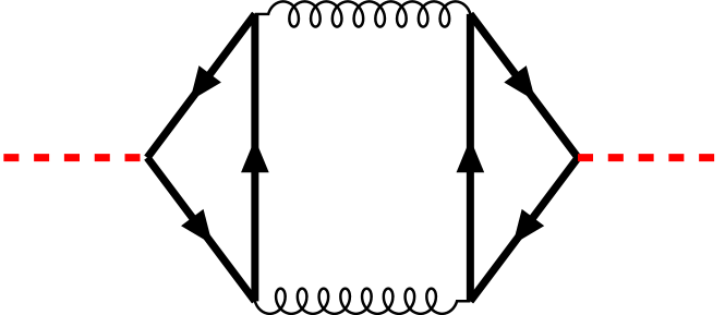
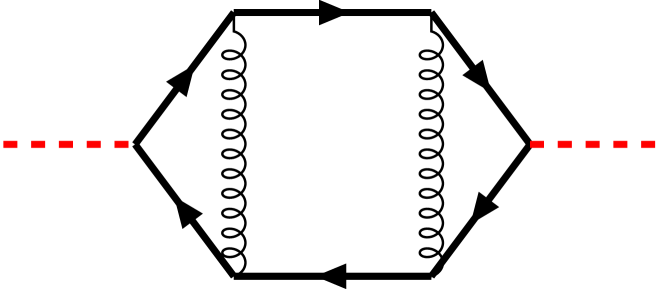
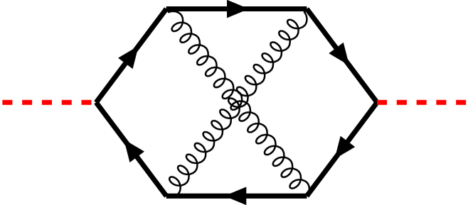
Figure 1: Typical three-loop Feynman diagrams of $H\rightarrow b\bar{b}\rightarrow H$. The thick black and red lines stand for the massive bottom quark and the Higgs boson, respectively.

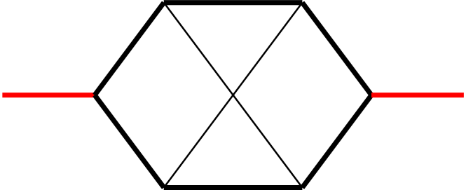
NP1

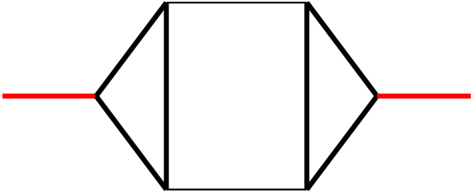
P1

Figure 2: The topologies of NP1 and P1 integral families. The thick black and red lines stand for the massive bottom quark and the Higgs boson, respectively. The other lines represent massless particles.

According to the cutting rules in the optical theorem, the imaginary parts of $\Sigma$ come from the cut diagrams in which some integral propagators are put on-shell simultaneously. We find that most cut diagrams in $\Sigma$ have at least two on-shell bottom-quark propagators. And these cut diagrams correspond to the processes $H\rightarrow b\bar{b}$, $H\rightarrow b\bar{b}g$, $H\rightarrow b\bar{b}gg$, $H\rightarrow b\bar{b}q\bar{q}$ and $H\rightarrow b\bar{b}b\bar{b}$. All of them contribute to $\Gamma_{Hbb}$ at $\mathcal{O}(y_{b}^{2}\alpha_{s}^{2})$. Two sample cut Feynman diagrams are shown in figure 3. The requirement of cuts on two bottom quarks simplifies the calculations since some MIs do not have imaginary parts, e.g., the three-loop massive vacuum bubble diagram shown in figure 4.

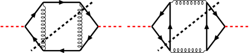
Figure 3: Typical cut diagrams. The black dashed line stands for the cut line, and the propagators crossing the cut line are on-shell. The cut line passes through two (left graph) and four (right graph) bottom quarks.

Figure 4: A three-loop massive vacuum bubble diagram.

Notice that some cut diagrams contribute to the imaginary part of $\Sigma$, but do not have two bottom-quark cut propagators, such as the diagram of a cut through two gluon propagators as depicted in figure 5. This cut diagram is related to the process $H\rightarrow gg$, which should not be included in the corrections of $H\rightarrow b\bar{b}$. To subtract this contribution from the imaginary part of the forward scattering amplitude, we calculate the squared amplitude of $H\rightarrow gg$ with one triangle bottom-quark loop, and perform the two-body phase space integration.

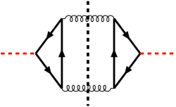
Figure 5: A cut diagram contributing to the $H\to gg$ decay.

3 Calculation of master integrals

As mentioned in eq.(2), we have to calculate the contributions from both two and four bottom quark final states. The corresponding MIs can be computed separately.

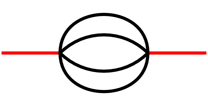
Figure 6: Two master integrals contributing to the decay to four bottom-quark final states. The thick black and red lines stand for the massive bottom quark and the Higgs boson, respectively.

The MIs contributing to the decay to four bottom quark final state contain elliptic integrals, such as those shown in figure 6. They have been calculated in Lee:2019wwn where the authors consider the total cross section of $e^{+}e^{-}\rightarrow Q\bar{Q}Q\bar{Q}$. After choosing a regular basis, only the $\mathcal{O}(\epsilon^{0})$ parts of the MIs are needed, which in turn can be expressed either as complete elliptic integrals of the first kind or one-fold integrals of them. Following this method, we present the decay width ${\Gamma}^{y_{b}y_{b}}_{Hb\bar{b}b\bar{b}}$ in terms of one-fold integrals over expressions depending on complete elliptic integrals and multiple polylogarithms. The explicit form can be found in eq. (33) below.

Then we turn to the MIs that are needed in the calculation of $\tilde{\Gamma}^{y_{b}y_{b}}_{Hb\bar{b}}$. We adopt the method of differential equations Kotikov:1990kg ; Kotikov:1991pm . Once a set of canonical basis $\bm{F}$ is found, the dimensional regulator $\epsilon$ is factorized out from the kinematic variables Henn:2013pwa ,

$$d\bm{F}(\epsilon,x_{n})=\epsilon\,dA(x_{n})\bm{F}(\epsilon,x_{n}),$$ (3)

where $\{x_{n}\}$ denote the kinematic variables. When $dA(x_{n})$ is expressed in $d\log$ forms, the differential equations can be solved recursively in terms of multiple polylogarithms (MPLs) Goncharov:1998kja , which are defined by $G(x)\equiv 1$ and

$$G(l_{1},l_{2},\ldots,l_{n},x) \equiv \int_{0}^{x}\frac{\text{d}t}{t-l_{1}}G(l_{2},\ldots,l_{n},t)\,,$$ (4)

$$G(\overrightarrow{0}_{n},x) \equiv \frac{1}{n!}\ln^{n}x\,.$$ (5)

The number of elements in the set $\{l_{1},l_{2},\ldots,l_{n}\}$ is referred to as the transcendental $weight$ of the MPLs. Note that we have dropped MIs that possess an imaginary part only from cuts on four bottom quarks. And all the boundary values are evaluated in the phase space where there are no possible cuts on four bottom quarks. For instance, the left diagram in figure 6 is dropped in the basis. The right diagram in figure 6 is included but only the cut through two bottom quarks, as shown in the right diagram of figure 7, is considered.

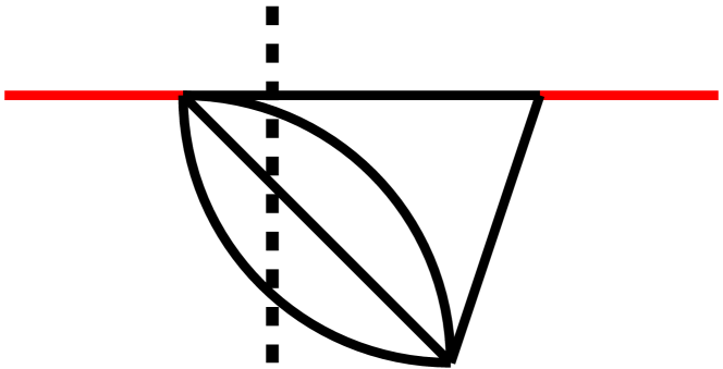
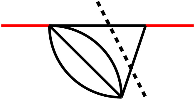
Figure 7: The four (left) and two (right) bottom quark cut diagrams. The thick black and red lines stand for the massive bottom quark and the Higgs boson, respectively.

3.1 Canonical basis of NP1

The master integrals of the NP1 integral family in figure 2 are defined by

$$I^{\rm NP1}_{n_{1},n_{2},\ldots,n_{9}}=\int{\mathcal{D}}^{D}q_{1}~{}{\mathcal{D}}^{D}q_{2}\frac{D_{9}^{-n_{9}}}{D_{1}^{n_{1}}~{}D_{2}^{n_{2}}~{}D_{3}^{n_{3}}~{}D_{4}^{n_{4}}~{}D_{5}^{n_{5}}~{}D_{6}^{n_{6}}~{}D_{7}^{n_{7}}D_{8}^{n_{8}}}$$ (6)

with

$${\mathcal{D}}^{D}q_{i}=\frac{\left(m_{b}^{2}\right)^{\epsilon}}{i\pi^{D/2}\Gamma(1+\epsilon)}d^{D}q_{i}\ ,\quad D=4-2\epsilon\,,$$ (7)

where all $n_{i}\geq 0,i=1,\cdots,8$, and $n_{9}\leq 0$. The denominators $D_{i}$ read

$$D_{1} =q_{1}^{2}-m_{b}^{2}, D_{2} =q_{2}^{2}-m_{b}^{2}, D_{3} =(q_{1}-q_{2})^{2},$$

$$D_{4} =q_{3}^{2}-m_{b}^{2}, D_{5} =(q_{2}+q_{3})^{2}, D_{6} =(q_{3}-k)^{2}-m_{b}^{2},$$

$$D_{7} =(q_{1}+k)^{2}-m_{b}^{2}, D_{8} =(q_{1}-q_{2}-q_{3}+k)^{2}-m_{b}^{2}, D_{9} =(q_{1}-q_{3}+k)^{2},$$ (8)

where the Feynman prescription $+i\varepsilon$ has been suppressed. The external momentum $k$ satisfies $k^{2}=m_{H}^{2}.$

In the NP1 integral family, there are 29 MIs contributing to $\tilde{\Gamma}_{Hb\bar{b}}$. To construct the canonical basis, we first select the MIs

$$\text{M}^{\text{NP1}}_{1} =\epsilon^{3}m_{b}^{2}I^{\text{NP1}}_{2,2,0,2,0,1,0,0,0},\quad \text{M}^{\text{NP1}}_{2} =\epsilon^{3}m_{b}^{2}I^{\text{NP1}}_{2,2,0,0,1,2,0,0,0},\quad$$

$$\text{M}^{\text{NP1}}_{3} =\epsilon^{3}m_{b}^{2}I^{\text{NP1}}_{2,2,0,0,2,1,0,0,0},\quad \text{M}^{\text{NP1}}_{4} =\epsilon^{3}m_{b}^{2}I^{\text{NP1}}_{2,0,2,0,1,2,0,0,0},\quad$$

$$\text{M}^{\text{NP1}}_{5} =\epsilon^{3}m_{b}^{2}I^{\text{NP1}}_{2,0,2,0,2,1,0,0,0},\quad \text{M}^{\text{NP1}}_{6} =(1-2\epsilon)\epsilon m_{b}^{4}I^{\text{NP1}}_{3,0,1,0,1,3,0,0,0},\quad$$

$$\text{M}^{\text{NP1}}_{7} =\epsilon^{3}m_{b}^{4}I^{\text{NP1}}_{2,2,0,2,0,1,1,0,0},\quad \text{M}^{\text{NP1}}_{8} =\epsilon^{3}m_{b}^{4}I^{\text{NP1}}_{0,2,1,2,0,1,2,0,0},\quad$$

$$\text{M}^{\text{NP1}}_{9} =\epsilon^{3}m_{b}^{4}I^{\text{NP1}}_{0,2,2,2,0,1,1,0,0},\quad \text{M}^{\text{NP1}}_{10} =\epsilon^{3}m_{b}^{2}I^{\text{NP1}}_{0,1,1,0,1,2,2,0,0},\quad$$

$$\text{M}^{\text{NP1}}_{11} =\epsilon^{2}m_{b}^{4}I^{\text{NP1}}_{0,1,1,0,1,3,2,0,0},\quad \text{M}^{\text{NP1}}_{12} =(1-2\epsilon)\epsilon^{3}m_{b}^{2}I^{\text{NP1}}_{0,2,1,0,1,2,1,0,0},\quad$$

$$\text{M}^{\text{NP1}}_{13} =(1-2\epsilon)\epsilon^{3}m_{b}^{2}I^{\text{NP1}}_{2,2,0,0,1,1,0,1,0},\quad \text{M}^{\text{NP1}}_{14} =\epsilon^{3}m_{b}^{4}I^{\text{NP1}}_{2,2,0,0,1,2,0,1,0},\quad$$

$$\text{M}^{\text{NP1}}_{15} =(1-2\epsilon)\epsilon^{3}m_{b}^{2}I^{\text{NP1}}_{2,0,2,1,1,1,0,0,0},\quad \text{M}^{\text{NP1}}_{16} =(1-2\epsilon)\epsilon^{3}m_{b}^{2}I^{\text{NP1}}_{2,2,0,1,0,1,0,1,0},\quad$$

$$\text{M}^{\text{NP1}}_{17} =(1-2\epsilon)\epsilon^{4}m_{b}^{2}I^{\text{NP1}}_{1,0,2,1,1,1,1,0,0},\quad \text{M}^{\text{NP1}}_{18} =(1-2\epsilon)\epsilon^{4}m_{b}^{2}I^{\text{NP1}}_{1,1,1,0,1,2,1,0,0},\quad$$

$$\text{M}^{\text{NP1}}_{19} =(1-2\epsilon)\epsilon^{4}m_{b}^{2}I^{\text{NP1}}_{2,1,0,1,1,1,0,1,0},\quad \text{M}^{\text{NP1}}_{20} =(1-2\epsilon)\epsilon^{3}m_{b}^{4}I^{\text{NP1}}_{2,1,0,1,1,1,0,2,0},\quad$$

$$\text{M}^{\text{NP1}}_{21} =(1-2\epsilon)\epsilon^{5}m_{b}^{2}I^{\text{NP1}}_{1,1,1,1,1,1,0,1,0},\quad \text{M}^{\text{NP1}}_{22} =(1-2\epsilon)^{2}\epsilon^{4}m_{b}^{2}I^{\text{NP1}}_{1,1,1,0,0,1,1,1,1},\quad$$

$$\text{M}^{\text{NP1}}_{23} =(1-2\epsilon)\epsilon^{4}m_{b}^{4}I^{\text{NP1}}_{1,1,1,0,0,1,2,1,1},\quad \text{M}^{\text{NP1}}_{24} =(1-2\epsilon)\epsilon^{4}m_{b}^{2}I^{\text{NP1}}_{1,2,0,1,0,1,1,1,0},\quad$$

$$\text{M}^{\text{NP1}}_{25} =(1-2\epsilon)\epsilon^{3}m_{b}^{4}I^{\text{NP1}}_{2,2,0,1,0,1,1,1,0},\quad \text{M}^{\text{NP1}}_{26} =(1-2\epsilon)\epsilon^{4}m_{b}^{4}I^{\text{NP1}}_{1,2,1,1,1,1,1,0,0},\quad$$

$$\text{M}^{\text{NP1}}_{27} =(1-2\epsilon)\epsilon^{4}m_{b}^{4}I^{\text{NP1}}_{2,1,1,1,1,1,1,0,0},\quad \text{M}^{\text{NP1}}_{28} =(1-2\epsilon)\epsilon^{5}m_{b}^{4}I^{\text{NP1}}_{1,1,1,1,1,1,1,1,0},\quad$$

$$\text{M}^{\text{NP1}}_{29} =(1-2\epsilon)\epsilon^{5}m_{b}^{2}I^{\text{NP1}}_{1,1,1,1,1,1,1,1,-1}\,.$$ (9)

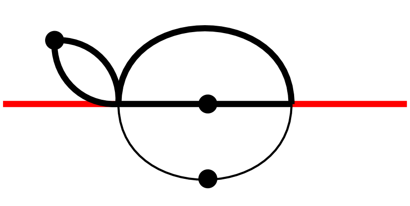
$\text{M}^{\text{NP1}}_{3}$

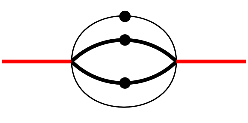
$\text{M}^{\text{NP1}}_{4}$

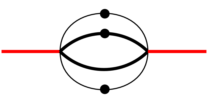
$\text{M}^{\text{NP1}}_{5}$

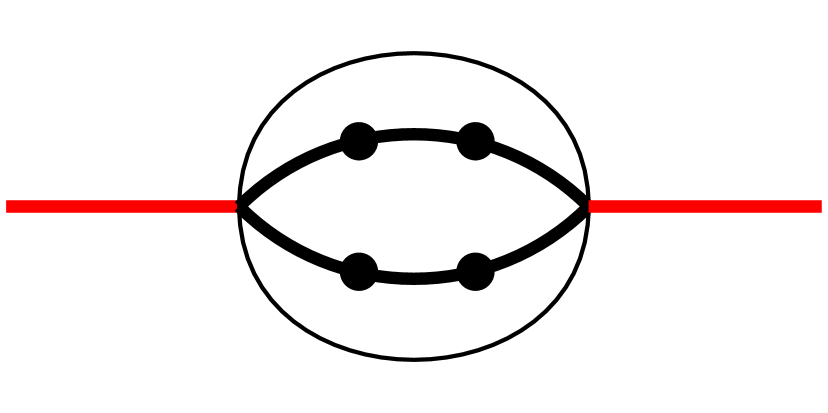
$\text{M}^{\text{NP1}}_{6}$

$\text{M}^{\text{NP1}}_{7}$

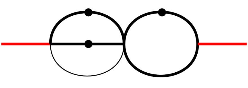
$\text{M}^{\text{NP1}}_{8}$

$\text{M}^{\text{NP1}}_{9}$

$\text{M}^{\text{NP1}}_{10}$

$\text{M}^{\text{NP1}}_{11}$

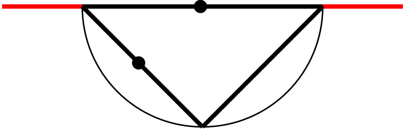
$\text{M}^{\text{NP1}}_{12}$

$\text{M}^{\text{NP1}}_{13}$

$\text{M}^{\text{NP1}}_{14}$

$\text{M}^{\text{NP1}}_{15}$

$\text{M}^{\text{NP1}}_{16}$

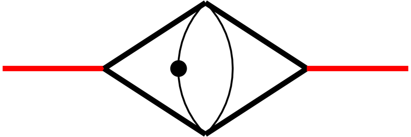
$\text{M}^{\text{NP1}}_{17}$

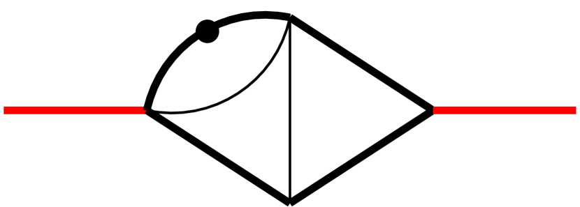
$\text{M}^{\text{NP1}}_{18}$

$\text{M}^{\text{NP1}}_{19}$

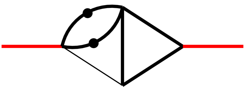
$\text{M}^{\text{NP1}}_{20}$

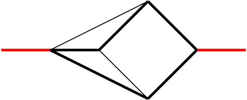
$\text{M}^{\text{NP1}}_{21}$

$\text{M}^{\text{NP1}}_{22}$

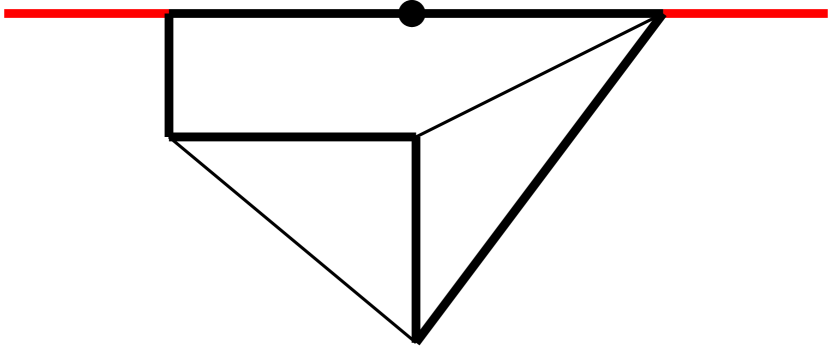
$\text{M}^{\text{NP1}}_{23}$

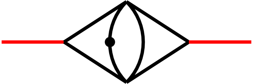
$\text{M}^{\text{NP1}}_{24}$

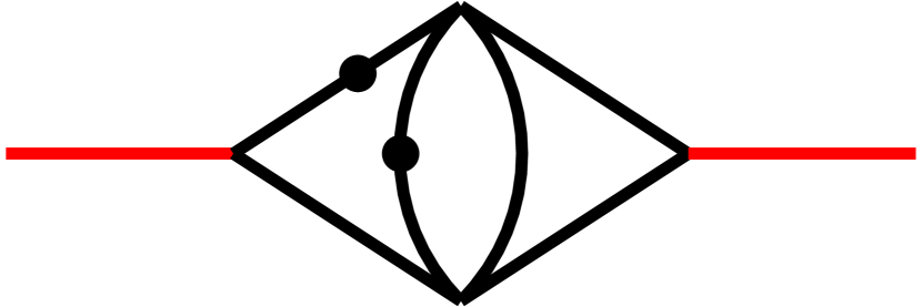
$\text{M}^{\text{NP1}}_{25}$

$\text{M}^{\text{NP1}}_{26}$

$\text{M}^{\text{NP1}}_{27}$

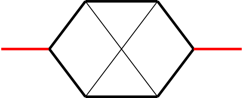
$\text{M}^{\text{NP1}}_{28}$, $\text{M}^{\text{NP1}}_{29}$

Figure 11: Master integrals in the NP1 topology. The thick black and red lines stand for the massive bottom quark and the Higgs boson, respectively. One black dot indicates one additional power of the corresponding propagator. The numerators can be found in the text.

Here all $\text{M}^{\text{NP1}}_{i}$ are dimensionless, and the corresponding topology diagrams are displayed in figure 11 in appendix A.

Then the canonical basis integrals $F^{\text{NP1}}_{i},~{}i=1,\dots,29,$ can be constructed as linear combinations of $\text{M}^{\text{NP1}}_{i}$ using a method similar to that in ref. Argeri:2014qva . Examples can be found in Chen:2021gjv . For simplicity, we define a dimensionless variable $z\equiv m_{H}^{2}/m_{b}^{2}+i0^{+}$. Then we obtain the following canonical basis of the NP1 family:

$$F^{\text{NP1}}_{1} =\text{M}^{\text{NP1}}_{1}r,\quad F^{\text{NP1}}_{2}=\text{M}^{\text{NP1}}_{2}\left(-z\right),\quad F^{\text{NP1}}_{3}=\frac{\text{M}^{\text{NP1}}_{2}r}{2}+\text{M}^{\text{NP1}}_{3}r,\quad$$

$$F^{\text{NP1}}_{4} =\text{M}^{\text{NP1}}_{4}\left(-z\right),\quad F^{\text{NP1}}_{5}=\left(\text{M}^{\text{NP1}}_{4}+\text{M}^{\text{NP1}}_{5}\right)(-r),\quad F^{\text{NP1}}_{6}=-\frac{\text{M}^{\text{NP1}}_{5}\left(4-z\right)}{4}+\text{M}^{\text{NP1}}_{6},\quad$$

$$F^{\text{NP1}}_{7} =\text{M}^{\text{NP1}}_{7}z\left(z-4\right),\quad F^{\text{NP1}}_{8}=\text{M}^{\text{NP1}}_{8}rz,\quad F^{\text{NP1}}_{9}=\frac{\text{M}^{\text{NP1}}_{8}\left(z-4\right)z}{2}+\text{M}^{\text{NP1}}_{9}\left(z-4\right)z,$$

$$F^{\text{NP1}}_{10} =\frac{\text{M}^{\text{NP1}}_{2}\left(4-3z\right)}{8-4z}+\frac{\text{M}^{\text{NP1}}_{4}z}{4}+\frac{\text{M}^{\text{NP1}}_{10}\left(2\epsilon\left(4z^{2}-9z-4\right)+4z^{2}-11z+4\right)}{8-4z}$$

$$\quad-\frac{2\text{M}^{\text{NP1}}_{11}\epsilon\left(2z-5\right)z}{z-2}+\frac{\text{M}^{\text{NP1}}_{12}\left(z-4\right)\left(z-1\right)}{4\left(z-2\right)},\quad$$

$$F^{\text{NP1}}_{11} =\frac{\text{M}^{\text{NP1}}_{2}r\left(z^{2}-6z+4\right)}{8\left(z-4\right)\left(z-2\right)}+\frac{\text{M}^{\text{NP1}}_{10}r\left(2\epsilon\left(z^{2}+2z-11\right)+z^{2}-4z+3\right)}{2\left(z-4\right)\left(z-2\right)}$$

$$\quad+\frac{\text{M}^{\text{NP1}}_{11}r\left(2\epsilon\left(z^{2}-6\right)-z+2\right)}{\left(z-4\right)\left(z-2\right)}-\frac{\text{M}^{\text{NP1}}_{12}r\left(z-3\right)\left(z-1\right)}{2\left(z-4\right)\left(z-2\right)},\quad$$

$$F^{\text{NP1}}_{12} =-\frac{\text{M}^{\text{NP1}}_{2}z}{z-2}+\text{M}^{\text{NP1}}_{4}z+\frac{\text{M}^{\text{NP1}}_{10}\left(6\epsilon z+z\right)}{2-z}-\frac{8\text{M}^{\text{NP1}}_{11}\epsilon z}{z-2}+\frac{\text{M}^{\text{NP1}}_{12}\left(z-1\right)z}{z-2},$$

$$F^{\text{NP1}}_{13} =\text{M}^{\text{NP1}}_{13}z+\text{M}^{\text{NP1}}_{14}z^{2},\quad F^{\text{NP1}}_{14}=\text{M}^{\text{NP1}}_{14}\left(-z\right),\quad$$

$$F^{\text{NP1}}_{15} =-\frac{\text{M}^{\text{NP1}}_{4}r\left(7z-12\right)}{12\left(4-z\right)}+\frac{\text{M}^{\text{NP1}}_{5}r}{12}-\frac{\text{M}^{\text{NP1}}_{6}r}{3\left(4-z\right)}+\frac{\text{M}^{\text{NP1}}_{15}r}{4-z},\quad F^{\text{NP1}}_{16}=-\frac{\text{M}^{\text{NP1}}_{16}r}{4-z},\quad$$

$$F^{\text{NP1}}_{17} =\text{M}^{\text{NP1}}_{17}\left(-z\right),\quad F^{\text{NP1}}_{18}=\text{M}^{\text{NP1}}_{18}\left(-z\right),\quad F^{\text{NP1}}_{19}=\text{M}^{\text{NP1}}_{19}\left(-z\right),$$

$$F^{\text{NP1}}_{20} =-2\text{M}^{\text{NP1}}_{14}rz-\frac{3\text{M}^{\text{NP1}}_{16}rz}{z-4}+\text{M}^{\text{NP1}}_{20}rz,\quad F^{\text{NP1}}_{21}=\text{M}^{\text{NP1}}_{21}z,$$

$$F^{\text{NP1}}_{22} =\frac{1}{4}z\left(\text{M}^{\text{NP1}}_{22}+\text{M}^{\text{NP1}}_{23}\left(z-4\right)\right),\quad$$

$$F^{\text{NP1}}_{23} =-\text{M}^{\text{NP1}}_{18}r+2\text{M}^{\text{NP1}}_{19}r+2\text{M}^{\text{NP1}}_{21}r+\text{M}^{\text{NP1}}_{22}r+\text{M}^{\text{NP1}}_{23}rz,\quad$$

$$F^{\text{NP1}}_{24} =\text{M}^{\text{NP1}}_{24}\left(-z\right),\quad F^{\text{NP1}}_{25}=-\frac{\text{M}^{\text{NP1}}_{16}rz}{z-4}+\text{M}^{\text{NP1}}_{25}rz,\quad F^{\text{NP1}}_{26}=\text{M}^{\text{NP1}}_{26}\left(-z\right),\quad$$

$$F^{\text{NP1}}_{27} =\frac{3\text{M}^{\text{NP1}}_{2}rz^{2}}{8\left(z-2\right)^{2}}+\frac{3\text{M}^{\text{NP1}}_{4}rz}{8\left(z-2\right)}-\frac{3\text{M}^{\text{NP1}}_{8}r\left(z-4\right)z}{8\left(z-2\right)}-\frac{3\text{M}^{\text{NP1}}_{9}r\left(z-4\right)z}{4\left(z-2\right)}$$

$$\quad+\frac{3\text{M}^{\text{NP1}}_{10}r(6\epsilon+1)z}{4\left(z-2\right)^{2}}+\frac{6\text{M}^{\text{NP1}}_{11}r\epsilon z}{\left(z-2\right)^{2}}-\frac{3\text{M}^{\text{NP1}}_{12}r\left(z-1\right)z}{4\left(z-2\right)^{2}}+\frac{3\text{M}^{\text{NP1}}_{17}rz}{2\left(z-2\right)}$$

$$\quad+\frac{\text{M}^{\text{NP1}}_{18}rz}{4\left(z-2\right)}+\frac{\text{M}^{\text{NP1}}_{26}rz}{z-2}-\frac{\text{M}^{\text{NP1}}_{27}rz}{z-2},\quad$$

$$F^{\text{NP1}}_{28} =\text{M}^{\text{NP1}}_{28}(-r)z,\quad F^{\text{NP1}}_{29}=\text{M}^{\text{NP1}}_{28}\left(z-4\right)z+\text{M}^{\text{NP1}}_{29}z,$$ (10)

where

$$r=\sqrt{z(z-4)}.$$ (11)

To rationalize the square root $r$, we write

$$z=-\frac{(w-1)^{2}}{w}$$ (12)

with $-1<w<0$. Then $r$ is rationalized to

$$r=\frac{(w+1)(w-1)}{w}.$$ (13)

The corresponding differential equations for the canonical basis $\bm{F}^{\text{NP1}}$ become

$$\frac{d\bm{F}^{\text{NP1}}}{dw}=\epsilon\left(\sum_{i=1}^{5}\frac{\bm{N_{i}}^{\text{NP1}}}{w-l_{i}^{\text{NP1}}}\right)\bm{F}^{\text{NP1}}$$ (14)

with

$$l^{\text{NP1}}_{1}=0\,,~{}l^{\text{NP1}}_{2}=1\,,~{}l^{\text{NP1}}_{3}=-1\,,~{}l^{\text{NP1}}_{4}=\frac{1+\sqrt{3}i}{2}\,,~{}l^{\text{NP1}}_{5}=\frac{1-\sqrt{3}i}{2}$$ (15)

and $\bm{N_{i}}^{\text{NP1}}$ being constant rational matrices.

3.2 Canonical basis of P1

The P1 integral family is defined by

$$I^{P1}_{n_{1},n_{2},\ldots,n_{9}}=\int{\mathcal{D}}^{D}q_{1}~{}{\mathcal{D}}^{D}q_{2}\frac{D_{9}^{-n_{9}}}{D_{1}^{n_{1}}~{}D_{2}^{n_{2}}~{}D_{3}^{n_{3}}~{}D_{4}^{n_{4}}~{}D_{5}^{n_{5}}~{}D_{6}^{n_{6}}~{}D_{7}^{n_{7}}D_{8}^{n_{8}}},$$ (16)

where the denominators $D_{i}$ read

$$D_{1} =q_{1}^{2}-m_{b}^{2}, D_{2} =(q_{1}+k_{1})^{2}-m_{b}^{2}, D_{3} =q_{3}^{2}-m_{b}^{2},$$

$$D_{4} =(q_{3}^{2}-k_{1})^{2}-m_{b}^{2}, D_{5} =(q_{1}-q_{2})^{2}-m_{b}^{2}, D_{6} =q_{2}^{2},$$

$$D_{7} =(q_{2}+q_{3})^{2}-m_{b}^{2}, D_{8} =(q_{2}+k_{1})^{2}, D_{9} =(q_{1}+q_{3})^{2}.$$ (17)

There are 19 MIs in this integral family contributing to $\tilde{\Gamma}_{Hb\bar{b}}$. Most of them have appeared in the NP1 integral family discussed above. Here we only show the new MIs,

$$\text{M}^{\text{P1}}_{1} =\epsilon^{3}m_{b}^{2}I^{\text{P1}}_{2,0,2,0,0,2,0,1,0},\quad \text{M}^{\text{P1}}_{5} =\epsilon^{3}m_{b}^{4}I^{\text{P1}}_{2,1,2,0,0,2,0,1,0},\quad$$

$$\text{M}^{\text{P1}}_{12} =\epsilon^{3}m_{b}^{6}I^{\text{P1}}_{2,1,2,1,0,2,0,1,0},\quad \text{M}^{\text{P1}}_{13} =(1-2\epsilon)\epsilon^{4}m_{b}^{2}I^{\text{P1}}_{1,1,2,0,1,1,0,1,0},\quad$$

$$\text{M}^{\text{P1}}_{18} =(1-2\epsilon)\epsilon^{4}m_{b}^{4}I^{\text{P1}}_{1,1,2,1,1,1,0,1,0},\quad \text{M}^{\text{P1}}_{19} =(1-2\epsilon)\epsilon^{5}m_{b}^{4}I^{\text{P1}}_{1,1,1,1,1,1,1,1,0}.\quad$$ (18)

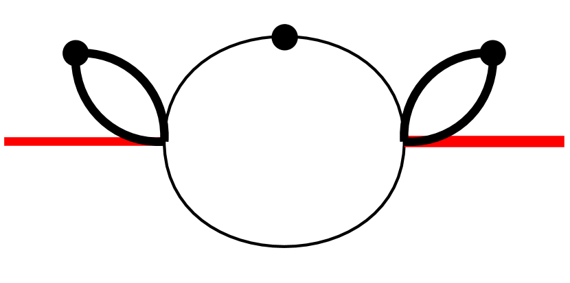
$\text{M}^{\text{P1}}_{1}$

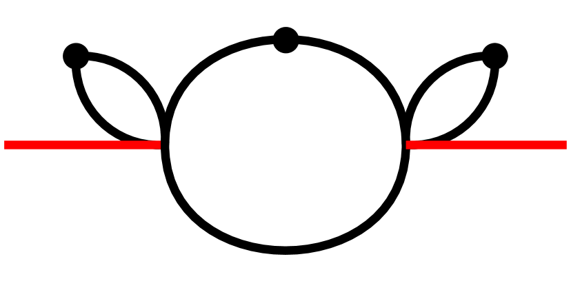
$\text{M}^{\text{P1}}_{2}$

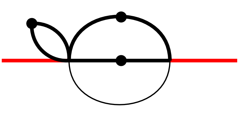
$\text{M}^{\text{P1}}_{3}$

$\text{M}^{\text{P1}}_{4}$

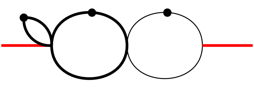
$\text{M}^{\text{P1}}_{5}$

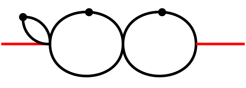
$\text{M}^{\text{P1}}_{6}$

$\text{M}^{\text{P1}}_{7}$

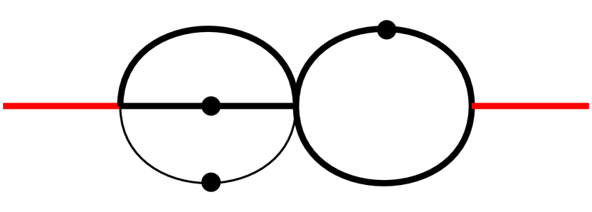
$\text{M}^{\text{P1}}_{8}$

$\text{M}^{\text{P1}}_{9}$

$\text{M}^{\text{P1}}_{10}$

$\text{M}^{\text{P1}}_{11}$

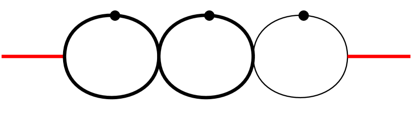
$\text{M}^{\text{P1}}_{12}$

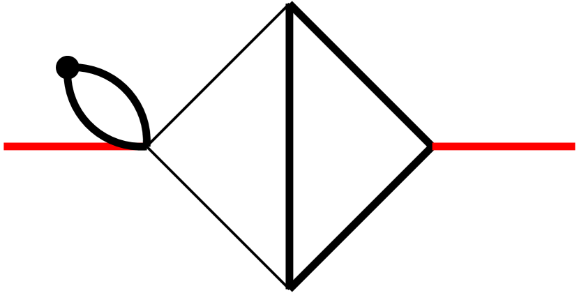
$\text{M}^{\text{P1}}_{13}$

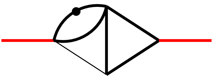
$\text{M}^{\text{P1}}_{14}$

$\text{M}^{\text{P1}}_{15}$

$\text{M}^{\text{P1}}_{16}$

$\text{M}^{\text{P1}}_{17}$

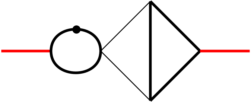
$\text{M}^{\text{P1}}_{18}$

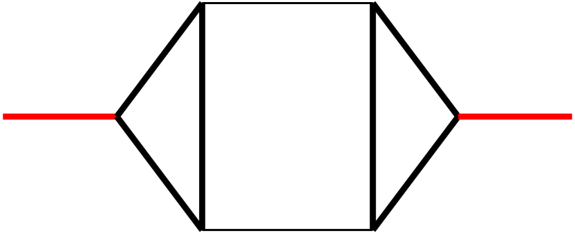
$\text{M}^{\text{P1}}_{19}$

Figure 12: Master integrals in the P1 topology. The thick black and red lines stand for the massive bottom quark and the Higgs boson, respectively. One black dot indicates one additional power of the corresponding propagator.

The topology diagrams are displayed in figure 12 in appendix A. We find the corresponding canonical basis integrals,

$$F^{\text{P1}}_{1} =\text{M}^{\text{P1}}_{1}\left(-z\right),\quad F^{\text{P1}}_{5}=\text{M}^{\text{P1}}_{5}(-r)z,\quad F^{\text{P1}}_{12}=-\text{M}^{\text{P1}}_{12}z^{2}\left(z-4\right),\quad$$

$$F^{\text{P1}}_{13} =\text{M}^{\text{P1}}_{13}\left(-z\right),\quad F^{\text{P1}}_{18}=\text{M}^{\text{P1}}_{18}(-r)z,\quad F^{\text{P1}}_{19}=\text{M}^{\text{P1}}_{19}z^{2}.$$ (19)

The corresponding differential equations are

$$\frac{d\bm{F}^{\text{P1}}}{dw}=\epsilon\left(\sum_{i=1}^{3}\frac{\bm{N_{i}}^{\text{P1}}}{w-l_{i}^{\text{P1}}}\right)\bm{F}^{\text{P1}}$$ (20)

with

$$l^{\text{P1}}_{1}=0\,,~{}l^{\text{P1}}_{2}=1\,,~{}l^{\text{P1}}_{3}=-1\,,~{}$$ (21)

and $\bm{N_{i}}^{\text{P1}}$ being constant rational matrices.

3.3 Boundary conditions

Given the above canonical differential equations, we obtain the results of the basis integrals at each order of $\epsilon$ up to some integration constants. The MPLs in the results can be evaluated efficiently using the PolyLogTools package Duhr:2019tlz , which depends on the algorithm of ref. Vollinga:2004sn in the GiNaC Bauer:2000cp framework. The integration constants are calculated numerically by comparing the results of basis integrals with those obtained using the AMFlow package Liu:2017jxz ; Liu:2020kpc ; Liu:2022chg . Their analytical form is reconstructed using the PSLQ algorithm Ferguson1992 ; Ferguson:1999aa . We find that the transcendental constants relevant to our calculation consist of

$$\{\log(2),\pi,\zeta(3)\}$$ (22)

up to weight four, where $\zeta(n)$ is the Riemann zeta function. All the master integrals are then checked against the numerical computation with AMFlow, and over 200-digit agreement is achieved. We provide the analytical results of the canonical bases in an ancillary file along with the arXiv submission.

4 Renormalization

In the framework of the optical theorem, the imaginary part of each three-loop self energy diagram arises from all possible cuts, corresponding to the sum of both virtual and real corrections. The infrared divergences cancel out in the sum, and only ultraviolet divergences remain.

We perform renormalization following the standard procedure, i.e., by including the contribution from diagrams with counter-terms. The bottom quark mass is renormalized in the on-shell scheme, while the strong coupling $\alpha_{s}$ is renormalized in the $\overline{\rm MS}$ scheme,

$$m_{b,bare} =Z_{m}m_{b},$$

$$\alpha_{s}^{bare}C^{\epsilon} =\mu^{2\epsilon}\alpha_{s}Z_{\alpha_{s}},$$ (23)

where $C_{\epsilon}=(4\pi e^{-\gamma_{E}})^{\epsilon}$. The renormalization constants up to $\alpha_{s}^{2}$ are given by Caswell:1974gg ; Jones:1974mm ; Czakon:2007wk ; Melnikov:2000qh ,

$$Z_{\alpha_{s}} =1+\left(\frac{\alpha_{s}}{4\pi}\right)\frac{2n_{l}-31}{3\epsilon}+\left(\frac{\alpha_{s}}{4\pi}\right)^{2}\left(\frac{\left(31-2n_{l}\right)^{2}}{9\epsilon^{2}}+\frac{19n_{l}-134}{3\epsilon}\right),$$

$$Z^{\overline{\rm MS}}_{m} =1-\left(\frac{\alpha_{s}}{4\pi}\right)\frac{4}{\epsilon}+\left(\frac{\alpha_{s}}{4\pi}\right)^{2}\left(\frac{2(43-2n_{l})}{3\epsilon^{2}}+\frac{10n_{l}-293}{9\epsilon}\right),$$

$$Z^{\text{OS}}_{m} =1+\left(\frac{\alpha_{s}}{4\pi}\right)D_{\epsilon}\left(-\frac{4}{\epsilon}-\frac{16}{3}-\frac{32\epsilon}{3}-\frac{64\epsilon^{2}}{3}\right)$$

$$\quad+\left(\frac{\alpha_{s}}{4\pi}\right)^{2}D_{\epsilon}^{2}\bigg{(}\frac{86-4n_{l}}{3\epsilon^{2}}+\frac{10n_{l}-101}{9\epsilon}+\frac{4\left(2n_{l}-31\right)}{3\epsilon}\log\left(\frac{\mu^{2}}{m^{2}}\right)$$

$$\quad+\frac{2(31-2n_{l})}{3}\log^{2}\left(\frac{\mu^{2}}{m^{2}}\right)+\frac{16(2n_{l}-31)}{9}\log\left(\frac{\mu^{2}}{m^{2}}\right)+\frac{\left(10n_{l}-79\right)\pi^{2}}{9}$$

$$\quad+\frac{\left(142n_{l}-2251\right)}{18}+\frac{8\zeta(3)}{3}-\frac{16\pi^{2}\log(2)}{9}\bigg{)},$$ (24)

where

$$D_{\epsilon}\equiv\frac{\Gamma(1+\epsilon)}{e^{-\gamma_{E}\epsilon}}\left(\frac{\mu^{2}}{m^{2}}\right)^{\epsilon}$$ (25)

and color factors $C_{F}=4/3$, $C_{A}=3$, $T_{R}=1/2$ have been substituted.

The bottom quark Yukawa coupling is related to the bottom quark mass. However, one has the freedom to choose a different renormalization scheme. Though it is expected that the final result for the decay width should be the same if all order corrections are included, the fixed-order results in different schemes may exhibit obvious deviations, which should be taken as one kind of theoretical uncertainty. The results with Yukawa couplings in the on-shell and $\overline{\rm MS}$ scheme can be converted to each other by applying the relations between the two schemes, which have been computed up to $\mathcal{O}(\alpha_{s}^{4})$ Broadhurst:1991fy ; Gray:1990yh ; Marquard:2015qpa ; Marquard:2016dcn . We have performed two separate calculations using different renormalization schemes. The ultraviolet divergences cancel in either scheme, and the final results agree with each other after the conversion of the renormalization scheme.

5 Analytic results

5.1 Full results

The decay width of $H\rightarrow b\bar{b}$ up to $\mathcal{O}(\alpha_{s}^{2})$ can be expressed as

$$\Gamma(H\rightarrow b\bar{b})=\Gamma_{\text{LO}}\left[1+\frac{\alpha_{s}(\mu)}{\pi}X_{1}^{y_{b}y_{b}}+\left(\frac{\alpha_{s}(\mu)}{\pi}\right)^{2}(X_{2}^{y_{b}y_{b}}+X_{2}^{y_{b}y_{t}})\right].$$ (26)

The LO result is

$$\Gamma_{\text{LO}}=\frac{N_{c}}{16\pi}\overline{y}_{b}^{2}m_{H}\left(1-\frac{4}{z}\right)^{3/2}\,,$$ (27)

where $N_{c}=3$ is the number of colors and $\overline{y}_{b}$ is the $\overline{\rm MS}$ Yukawa coupling

$$\overline{y}_{b}(\mu)=\overline{m_{b}}(\mu)\left(2\sqrt{2}G_{F}\right)^{1/2}$$ (28)

with $\overline{m_{b}}$ the $\overline{\rm MS}$ mass of the bottom quark and $G_{F}$ the Fermi constant.

The NLO coefficient $X_{1}^{y_{b}y_{b}}$ reads

$$X_{1}^{y_{b}y_{b}}(w)=2\log\left(\frac{\mu^{2}}{m_{H}^{2}}\right)+\frac{8}{3(w^{2}-1)}\Big{\{}2\left(-w^{2}+i\pi\left(w^{2}+1\right)+1\right)G(-1,w)$$

$$\quad+\frac{1}{2}\left(w^{2}+2i\pi\left(w^{2}+1\right)-1\right)G(1,w)+\frac{w\left(3w^{3}-w^{2}-8w-7\right)G(0,w)}{2(w+1)^{2}}$$

$$\quad+\left(w^{2}+1\right)\left(-2G(-1,0,w)+2G(0,-1,w)+G(0,1,w)-G(1,0,w)\right)$$

$$\quad+\frac{(17-12i\pi)w^{4}+(40+4i\pi)w^{3}+32i\pi w^{2}+(-40+28i\pi)w-17}{8(w+1)^{2}}\Big{\}}.$$ (29)

Though there are $i\pi$ terms in the expression, the full result is real since the MPLs also contain imaginary parts.

The $\mathcal{O}(\alpha_{s}^{2})$ corrections include two parts, i.e., $X_{2}^{y_{b}y_{b}}$ and $X_{2}^{y_{b}y_{t}}$. The latter denotes the contribution from the interference of the bottom and top quark Yukawa coupling induced amplitudes and starts at $\mathcal{O}(\alpha_{s}^{2})$. The corresponding analytical result has been calculated in ref. Primo:2018zby . The former receives contributions from both two and four bottom quark final states, as discussed in section 2,

$$X_{2}^{y_{b}y_{b}}=\tilde{X}_{2,b\bar{b}}^{y_{b}y_{b}}+X_{2,b\bar{b}b\bar{b}}^{y_{b}y_{b}}\,.$$ (30)

The result of $\tilde{X}_{2,b\bar{b}}^{y_{b}y_{b}}$ is given by

$$\tilde{X}_{2,b\bar{b}}^{y_{b}y_{b}}(w)=-\frac{4\left(w^{2}+1\right)^{2}}{9\left(w^{2}-1\right)^{2}}\Big{\{}100G(0,-1,-1,0,w)+28G(0,-1,0,-1,w)+14G(0,-1,0,1,w)$$

$$\quad+76G(0,-1,1,0,w)-128G(0,0,-1,-1,w)-64G(0,0,-1,1,w)-64G(0,0,1,-1,w)$$

$$\quad-32G(0,0,1,1,w)+76G(0,1,-1,0,w)-4G(0,1,0,-1,w)-2G(0,1,0,1,w)$$

$$\quad+35G(0,1,1,0,w)\Big{\}}-\frac{32\left(w^{4}+10w^{2}+1\right)}{9(w-1)(w+1)^{3}}\Big{\{}-6G(1,x_{1},0,-1,w)+4G(1,x_{1},0,0,w)$$

$$\quad-3G(1,x_{1},0,1,w)+G(1,x_{1},1,0,w)-6G(1,x_{2},0,-1,w)+4G(1,x_{2},0,0,w)$$

$$\quad-3G(1,x_{2},0,1,w)+G(1,x_{2},1,0,w)+6G(1,0,0,-1,w)+3G(1,0,0,1,w)$$

$$\quad-G(1,0,1,0,w)\Big{\}}-\frac{32\left(2w^{5}+w^{4}+8w^{3}-2w^{2}+2w+1\right)}{9(w-1)^{2}(w+1)^{3}}\Big{\{}6G(0,x_{1},0,-1,w)$$

$$\quad-4G(0,x_{1},0,0,w)+3G(0,x_{1},0,1,w)-G(0,x_{1},1,0,w)+6G(0,x_{2},0,-1,w)$$

$$\quad-4G(0,x_{2},0,0,w)+3G(0,x_{2},0,1,w)-G(0,x_{2},1,0,w)\Big{\}}$$

$$\quad+\frac{1}{9\left(w^{2}-1\right)^{3}}\Big{\{}-8\left(w^{4}-w^{3}-16w^{2}-w+1\right)(w-1)^{2}G(1,0,0,0,w)$$

$$\quad-16w\left(6w^{4}+2w^{3}+31w^{2}-19w+4\right)(w-1)G(0,0,0,-1,w)$$

$$\quad+w\left(6w^{5}-30w^{4}-113w^{3}-194w^{2}-119w-30\right)G(0,0,0,0,w)$$

$$\quad-4w\left(12w^{5}+w^{4}+94w^{3}-46w^{2}+82w+1\right)G(0,0,0,1,w)$$

$$\quad+4\left(90w^{6}-96w^{5}+741w^{4}-1226w^{3}+523w^{2}-96w-128\right)G(0,-1,0,0,w)$$

$$\quad+32\left(6w^{6}+4w^{5}-35w^{4}+94w^{3}-33w^{2}+4w+8\right)G(0,0,-1,0,w)$$

$$\quad+2\left(94w^{6}+48w^{5}-431w^{4}+1118w^{3}-413w^{2}+48w+112\right)G(0,0,1,0,w)$$

$$\quad+2\left(29w^{6}-60w^{5}+959w^{4}-1628w^{3}+749w^{2}-60w-181\right)G(0,1,0,0,w)\Big{\}}$$

$$\quad+\frac{\pi^{4}\left(231w^{6}-528w^{5}-1774w^{4}-5226w^{3}-1986w^{2}-528w+19\right)}{1620\left(w^{2}-1\right)^{3}}$$

$$\quad-\frac{4i\pi^{3}\left(w^{4}-w^{3}-16w^{2}-w+1\right)G(1,w)}{9(w-1)(w+1)^{3}}$$

$$\quad+\frac{256\pi^{2}\left(w^{4}+10w^{2}+1\right)(G(1,x_{1},w)+G(1,x_{2},w))}{27(w-1)(w+1)^{3}}$$

$$\quad-\frac{256\pi^{2}\left(2w^{5}+w^{4}+8w^{3}-2w^{2}+2w+1\right)(G(0,x_{1},w)+G(0,x_{2},w))}{27(w-1)^{2}(w+1)^{3}}$$

$$\quad+\frac{i\pi^{3}w\left(10w^{5}-18w^{4}-65w^{3}-26w^{2}-75w-18\right)G(0,w)}{27\left(w^{2}-1\right)^{3}}$$

$$\quad+\frac{2\pi^{2}}{27\left(w^{2}-1\right)^{3}}\Big{\{}10\left(w^{4}-w^{3}-16w^{2}-w+1\right)(w-1)^{2}G(1,0,w)$$

$$\quad-w\left(8w^{5}-24w^{4}-89w^{3}-110w^{2}-97w-24\right)G(0,0,w)$$

$$\quad-\left(361w^{6}-384w^{5}+2956w^{4}-4698w^{3}+2084w^{2}-384w-511\right)G(0,-1,w)$$

$$\quad-3\left(19w^{6}-40w^{5}+642w^{4}-1154w^{3}+502w^{2}-40w-121\right)G(0,1,w)\Big{\}}$$

$$\quad-\frac{32\left(w^{4}+10w^{2}+1\right)\zeta(3)G(1,w)}{3(w-1)(w+1)^{3}}$$

$$\quad-\frac{2\left(15w^{6}-18w^{5}-78w^{4}+386w^{3}-94w^{2}-18w-1\right)\zeta(3)G(0,w)}{9\left(w^{2}-1\right)^{3}}$$

$$\quad-\frac{32i\pi\left(w^{4}+10w^{2}+1\right)}{9(w-1)(w+1)^{3}}\Big{\{}-4G(1,x_{1},0,w)-G(1,x_{1},1,w)-4G(1,x_{2},0,w)$$

$$\quad-G(1,x_{2},1,w)+G(1,0,1,w)\Big{\}}-\frac{32i\pi\left(2w^{5}+w^{4}+8w^{3}-2w^{2}+2w+1\right)}{9(w-1)^{2}(w+1)^{3}}\Big{\{}4G(0,x_{1},0,w)$$

$$\quad+G(0,x_{1},1,w)+4G(0,x_{2},0,w)+G(0,x_{2},1,w)\Big{\}}+\frac{4i\pi\left(w^{2}+1\right)^{2}}{9\left(w^{2}-1\right)^{2}}\Big{\{}100G(0,-1,-1,w)$$

$$\quad+76G(0,-1,1,w)+76G(0,1,-1,w)+35G(0,1,1,w)\Big{\}}$$

$$\quad+\frac{\pi i}{9\left(w^{2}-1\right)^{3}}\Big{\{}-w\left(6w^{5}-30w^{4}-113w^{3}-194w^{2}-119w-30\right)G(0,0,0,w)$$

$$\quad-4\left(90w^{6}-96w^{5}+741w^{4}-1226w^{3}+523w^{2}-96w-128\right)G(0,-1,0,w)$$

$$\quad-32\left(6w^{6}+4w^{5}-35w^{4}+94w^{3}-33w^{2}+4w+8\right)G(0,0,-1,w)$$

$$\quad-2\left(94w^{6}+48w^{5}-431w^{4}+1118w^{3}-413w^{2}+48w+112\right)G(0,0,1,w)$$

$$\quad-2\left(29w^{6}-60w^{5}+959w^{4}-1628w^{3}+749w^{2}-60w-181\right)G(0,1,0,w)$$

$$\quad+2\left(15w^{6}-18w^{5}-78w^{4}+386w^{3}-94w^{2}-18w-1\right)\zeta(3)\Big{\}}$$

$$\quad+\frac{8i\pi\left(w^{4}-w^{3}-16w^{2}-w+1\right)G(1,0,0,w)}{9(w-1)(w+1)^{3}}$$

$$\quad+\frac{2(2n_{l}-55)(w^{2}+1)}{9\left(w^{2}-1\right)}\log\left(\frac{\mu^{2}}{m_{H}^{2}}\right)\Big{\{}-2i\pi G(-1,w)-i\pi G(1,w)+2G(-1,0,w)$$

$$\quad-2G(0,-1,w)-G(0,1,w)+G(1,0,w)\Big{\}}+\frac{4\left(w^{2}+1\right)}{9(w-1)(w+1)}\Big{\{}(166-4n_{l})G(-1,-1,0,w)$$

$$\quad+(94-4n_{l})G(-1,0,-1,w)+(110-4n_{l})G(-1,0,0,w)+(2n_{l}-63)G(-1,0,1,w)$$

$$\quad+(4n_{l}-34)G(-1,1,0,w)+(8n_{l}-260)G(0,-1,-1,w)+(4n_{l}-110)G(0,0,-1,w)$$

$$\quad+(2n_{l}-55)G(0,0,1,w)+(45-2n_{l})G(0,1,1,w)+(4n_{l}-34)G(1,-1,0,w)$$

$$\quad+(110-4n_{l})G(1,0,-1,w)+(55-2n_{l})G(1,0,0,w)+(4n_{l}-110)G(1,1,0,w)$$

$$\quad-20G(0,-1,1,w)-20G(0,1,-1,w)\Big{\}}$$

$$\quad+\frac{31w^{4}+86w^{3}-49w^{2}+86w+31}{9(w-1)(w+1)^{3}}\Big{\{}6G(x_{1},0,-1,w)-4G(x_{1},0,0,w)+3G(x_{1},0,1,w)$$

$$\quad-G(x_{1},1,0,w)+6G(x_{2},0,-1,w)-4G(x_{2},0,0,w)+3G(x_{2},0,1,w)-G(x_{2},1,0,w)\Big{\}}$$

$$\quad+\frac{4n_{l}\left(w^{5}+w^{4}-w-1\right)-118w^{5}+480w^{4}-459w^{3}+331w^{2}+628w+162}{9(w-1)^{2}(w+1)^{3}}$$

$$\quad\times\Big{\{}2G(0,0,-1,w)-G(0,0,1,w)\Big{\}}+\frac{1}{18(w-1)^{2}(w+1)^{3}}$$

$$\quad\times\Big{\{}2(w+1)\left(20n_{l}\left(w^{4}-1\right)-383w^{4}+1586w^{3}-2786w^{2}+1586w+1149\right)G(-1,0,0,w)$$

$$\quad-32(w+1)\left(n_{l}\left(w^{4}-1\right)+3w^{4}+32w^{3}-123w^{2}+32w+40\right)G(0,-1,0,w)$$

$$\quad+8(w-1)\left(-4n_{l}(w+1)^{2}\left(w^{2}+1\right)+63w^{4}+120w^{3}+130w^{2}+120w+63\right)G(1,0,-1,w)$$

$$\quad-(w-1)\left(-24n_{l}(w+1)^{2}\left(w^{2}+1\right)+183w^{4}-1220w^{3}+1662w^{2}+4444w+1459\right)G(1,0,0,w)$$

$$\quad+2(w-1)\left(-8n_{l}(w+1)^{2}\left(w^{2}+1\right)+126w^{4}+240w^{3}+260w^{2}+240w+126\right)G(1,0,1,w)$$

$$\quad-8\left(4n_{l}\left(w^{5}+w^{4}-w-1\right)-118w^{5}+480w^{4}-459w^{3}+331w^{2}+628w+162\right)G(0,0,-1,w)$$

$$\quad-2\left(12n_{l}\left(w^{5}+w^{4}-w-1\right)+89w^{5}+319w^{4}-1018w^{3}-1278w^{2}+760w+488\right)G(0,1,0,w)$$

$$\quad+2(w-1)\left(139w^{4}+284w^{3}+274w^{2}+284w+139\right)G(1,1,0,w)$$

$$\quad+\left(-11w^{5}-43w^{4}-203w^{3}-157w^{2}+26w+4\right)G(0,0,0,w)\Big{\}}$$

$$\quad+\frac{8i\pi\left(w^{2}+1\right)}{9\left(w^{2}-1\right)}\Big{\{}(2n_{l}-83)G(-1,-1,w)-(2n_{l}-17)G(-1,1,w)-(2n_{l}-17)G(1,-1,w)\Big{\}}$$

$$\quad+\frac{i\pi\left(31w^{4}+86w^{3}-49w^{2}+86w+31\right)}{9(w-1)(w+1)^{3}}\Big{\{}4G(x_{1},0,w)+G(x_{1},1,w)+4G(x_{2},0,w)$$

$$\quad+G(x_{2},1,w)\Big{\}}+\frac{8\pi^{2}\left(31w^{4}+86w^{3}-49w^{2}+86w+31\right)}{27(w-1)(w+1)^{3}}\Big{\{}G(x_{1},w)+G(x_{2},w)\Big{\}}$$

$$\quad-\frac{i\pi^{3}\left(22w^{5}+66w^{4}+205w^{3}+131w^{2}-37w-3\right)}{54(w-1)^{2}(w+1)^{3}}+\frac{2\left(w^{2}-4w+1\right)\pi^{2}\log(2)}{9(w+1)^{2}}$$

$$\quad-\frac{\left(6n_{l}\left(w^{5}+w^{4}-w-1\right)-159w^{5}+317w^{4}+44w^{3}+844w^{2}+510w+172\right)\zeta(3)}{9(w-1)^{2}(w+1)^{3}}$$

$$\quad+\frac{\pi^{2}}{54(w-1)^{2}(w+1)^{3}}\Big{\{}-(w+1)(32n_{l}\left(w^{4}-1\right)-217w^{4}+6354w^{3}-10770w^{2}$$

$$\quad+6354w+3271)G(-1,w)+\left(33w^{5}+109w^{4}+408w^{3}+288w^{2}-63w-7\right)G(0,w)$$

$$\quad-\left(24n_{l}\left(w^{5}+w^{4}-w-1\right)+311w^{5}+3473w^{4}-6172w^{3}-5972w^{2}+5317w+2275\right)G(1,w)\Big{\}}$$

$$\quad+\frac{i\pi}{18(w-1)^{2}(w+1)^{3}}\Big{\{}-2(w+1)(4n_{l}\left(w^{4}-1\right)+57w^{4}+1586w^{3}-2786w^{2}$$

$$\quad+1586w+709)G(-1,0,w)+32(w+1)\left(n_{l}\left(w^{4}-1\right)+3w^{4}+32w^{3}-123w^{2}+32w+40\right)$$

$$\quad\times G(0,-1,w)+\left(11w^{5}+43w^{4}+203w^{3}+157w^{2}-26w-4\right)G(0,0,w)$$

$$\quad+2\left(12n_{l}\left(w^{5}+w^{4}-w-1\right)+89w^{5}+319w^{4}-1018w^{3}-1278w^{2}+760w+488\right)G(0,1,w)$$

$$\quad-\left(8n_{l}\left(w^{5}+w^{4}-w-1\right)+257w^{5}+1843w^{4}-2882w^{3}-2782w^{2}+2545w+1019\right)G(1,0,w)$$

$$\quad+\left(-32n_{l}\left(w^{5}+w^{4}-w-1\right)+602w^{5}+590w^{4}+20w^{3}-20w^{2}-590w-602\right)G(1,1,w)\Big{\}}$$

$$\quad-\frac{2n_{l}-55}{12}\log^{2}\left(\frac{\mu^{2}}{m_{H}^{2}}\right)+\frac{2n_{l}-55}{9}\log\left(\frac{\mu^{2}}{m_{H}^{2}}\right)\Big{(}4G(-1,w)-G(1,w)\Big{)}$$

$$\quad+\frac{i(2n_{l}-55)w\left(3w^{3}-w^{2}-8w-7\right)}{9(w-1)(w+1)^{3}}\log\left(\frac{\mu^{2}}{m_{H}^{2}}\right)\Big{(}\pi+iG(0,w)\Big{)}$$

$$\quad-\frac{2}{9}\Big{\{}16n_{l}G(-1,-1,w)+2n_{l}G(1,1,w)-392G(-1,-1,w)+24G(-1,1,w)$$

$$\quad+24G(1,-1,w)-43G(1,1,w)\Big{\}}-\frac{2w}{3\left(w^{2}-1\right)}\Big{\{}-2G(0,0,w)+2i\pi G(0,w)\Big{\}}$$

$$\quad+\frac{8\left(n_{l}\left(11w^{2}-12w-1\right)-321w^{2}+471w-45\right)}{27\left(w^{2}-1\right)}G(-1,0,w)$$

$$\quad+\frac{1}{27(w-1)\left(w^{3}+1\right)^{3}}\Big{\{}\Big{(}4n_{l}\left(w^{2}-w+1\right)^{3}\left(11w^{4}+4w^{3}-20w^{2}-44w-13\right)$$

$$\quad-6(41w^{10}-626w^{9}+957w^{8}-2300w^{7}+2753w^{6}-4566w^{5}+3857w^{4}-3404w^{3}$$

$$\quad+957w^{2}-258w-327)\Big{)}G(0,-1,w)+\Big{(}-2n_{l}(w+1)^{2}\left(w^{2}-w+1\right)^{3}\left(7w^{2}-24w+13\right)$$

$$\quad+3(289w^{10}-450w^{9}+449w^{8}+1224w^{7}-2925w^{6}+4408w^{5}-3039w^{4}+1338w^{3}$$

$$\quad+449w^{2}-488w+327)\Big{)}G(0,1,w)+\Big{(}-4n_{l}\left(w^{2}-w+1\right)^{3}\left(w^{4}-w^{3}-28w^{2}+5w+4\right)$$

$$\quad+3(57w^{10}-245w^{9}-516w^{8}+2349w^{7}-5403w^{6}+6486w^{5}-5517w^{4}+2463w^{3}-516w^{2}$$

$$\quad-283w+95)\Big{)}G(1,0,w)\Big{\}}+\frac{G(0,0,w)}{54(w-1)^{2}(w+1)^{4}\left(w^{2}-w+1\right)^{3}}$$

$$\quad\times\Big{\{}-2(6n_{l}+527)w^{12}+(336n_{l}-12575)w^{11}+(32735-936n_{l})w^{10}+24(57n_{l}-2240)w^{9}$$

$$\quad+(31063-756n_{l})w^{8}+(12305-684n_{l})w^{7}+4(423n_{l}-12790)w^{6}+(44291-1440n_{l})w^{5}$$

$$\quad+(360n_{l}-15539)w^{4}+24(13n_{l}-174)w^{3}+(6221-348n_{l})w^{2}+(108n_{l}-1061)w+38\Big{\}}$$

$$\quad+\frac{\pi^{2}}{54(w-1)^{2}(w+1)^{4}\left(w^{2}-w+1\right)^{3}}\Big{\{}n_{l}\left(w^{2}-w+1\right)^{3}(23w^{6}-162w^{5}-71w^{4}+164w^{3}$$

$$\quad+45w^{2}-2w+3)+281w^{12}+9318w^{11}-21794w^{10}+34216w^{9}-18084w^{8}-7596w^{7}$$

$$\quad+31012w^{6}-26382w^{5}+11106w^{4}-160w^{3}-1732w^{2}-84w-117\Big{\}}$$

$$\quad-\frac{8i\pi\left(n_{l}\left(11w^{2}-12w-1\right)-321w^{2}+471w-45\right)}{27\left(w^{2}-1\right)}G(-1,w)$$

$$\quad+\frac{i\pi}{54(w-1)^{2}(w+1)^{4}\left(w^{2}-w+1\right)^{3}}\Big{\{}2(6n_{l}+527)w^{12}+(12575-336n_{l})w^{11}$$

$$\quad+(936n_{l}-32735)w^{10}-24(57n_{l}-2240)w^{9}+(756n_{l}-31063)w^{8}+(684n_{l}-12305)w^{7}$$

$$\quad+(51160-1692n_{l})w^{6}+(1440n_{l}-44291)w^{5}+(15539-360n_{l})w^{4}+(4176-312n_{l})w^{3}$$

$$\quad+(348n_{l}-6221)w^{2}+(1061-108n_{l})w-38\Big{\}}G(0,w)$$

$$\quad+\frac{i\pi}{27(w-1)\left(w^{3}+1\right)^{3}}\Big{\{}4n_{l}\left(w^{2}-w+1\right)^{3}\left(w^{4}-w^{3}-28w^{2}+5w+4\right)$$

$$\quad-3(57w^{10}-245w^{9}-516w^{8}+2349w^{7}-5403w^{6}+6486w^{5}-5517w^{4}$$

$$\quad+2463w^{3}-516w^{2}-283w+95)\Big{\}}G(1,w)$$

$$\quad-\frac{\left(n_{l}\left(22w^{2}+50w+22\right)-614w^{2}-1393w-614\right)}{18(w+1)^{2}}\log\left(\frac{\mu^{2}}{m_{H}^{2}}\right)$$

$$\quad+\frac{1}{27\left(w^{3}+1\right)^{2}}\Big{\{}2n_{l}\left(w^{2}-w+1\right)^{2}\left(59w^{2}+136w+59\right)$$

$$\quad-3\left(993w^{6}+736w^{5}-1424w^{4}+4130w^{3}-1424w^{2}+736w+993\right)\Big{\}}G(-1,w)$$

$$\quad+\frac{1}{324(w-1)(w+1)^{3}\left(w^{2}-w+1\right)^{2}}\Big{\{}(31015-1332n_{l})w^{8}+6(170n_{l}-2271)w^{7}$$

$$\quad+(1440n_{l}-81929)w^{6}+(192374-5112n_{l})w^{5}+6(916n_{l}-34731)w^{4}-22(72n_{l}-2963)w^{3}$$

$$\quad+(14605-756n_{l})w^{2}+6(242n_{l}-7905)w-503\Big{\}}G(0,w)$$

$$\quad+\frac{1}{54(w+1)^{2}\left(w^{2}-w+1\right)^{2}}\Big{\{}3\left(235w^{6}-406w^{5}+764w^{4}-684w^{3}+764w^{2}-406w+235\right)$$

$$\quad-14n_{l}\left(w^{3}+1\right)^{2}\Big{\}}G(1,w)+\frac{i\pi}{324(w-1)(w+1)^{3}\left(w^{2}-w+1\right)^{2}}\Big{\{}(1332n_{l}-31015)w^{8}$$

$$\quad-6(170n_{l}-2271)w^{7}+(81929-1440n_{l})w^{6}+2(2556n_{l}-96187)w^{5}-6(916n_{l}-34731)w^{4}$$

$$\quad+22(72n_{l}-2963)w^{3}+(756n_{l}-14605)w^{2}-6(242n_{l}-7905)w+503\Big{\}}$$

$$\quad+\frac{-18n_{l}\left(195w^{2}+374w+195\right)+98681w^{2}+204550w+98681}{1296(w+1)^{2}}$$ (31)

with

$$x_{1}=l^{\text{NP1}}_{4}=\frac{1+\sqrt{3}i}{2},\quad x_{2}=l^{\text{NP1}}_{5}=\frac{1-\sqrt{3}i}{2}\,.$$ (32)

Here the color factors $C_{F}=4/3$, $C_{A}=3$, and $T_{R}=1/2$ have been substituted by their numeric values, and $n_{l}$ denotes the number of light quark flavors.

The result of $X_{2,b\bar{b}b\bar{b}}^{y_{b}y_{b}}$ is given by

$$X_{2,b\bar{b}b\bar{b}}^{y_{b}y_{b}} =\frac{8}{3\pi\beta(z-4)z}\Big{\{}\frac{F^{4b}_{1}\left(-207z^{2}-3964z-11264\right)}{55296}+\frac{F^{4b}_{2}\left(479z^{2}+18860z-34528\right)}{82944}$$

$$\quad-\frac{F^{4b}_{3}(z-4)(2491z+3012)}{20736}+\frac{F^{4b}_{4}\left(-55z^{3}+254z^{2}+2328z-9216\right)}{3456\beta z}$$

$$\quad+\frac{F^{4b}_{5}\left(-5z^{2}+24z-32\right)}{2304}+\frac{\beta F^{4b}_{6}\left(-5z^{2}+10z+384\right)}{1152}+\frac{F^{4b}_{7}\left(5z^{2}-42z+90\right)}{576}$$

$$\quad+\frac{\beta F^{4b}_{8}\left(17z^{2}-58z-384\right)}{1152}+\frac{F^{4b}_{9}\left(z^{3}-6z^{2}+z-192\right)}{288z}+\frac{F^{4b}_{10}\left(z^{2}-3z-16\right)}{144}$$

$$\quad-\frac{\beta F^{4b}_{12}(z-2)^{2}}{144}\Big{\}}\,,$$ (33)

where $\beta=\sqrt{1-4/z}$ measures the velocity of the bottom quark. The master integrals $F^{4b}_{1}$, $F^{4b}_{2}$ and $F^{4b}_{3}$ are linear combinations of complete elliptic integrals or their derivatives, and the other $F^{4b}_{i}$ can be expressed by one-fold integrals of MPLs and complete elliptic integrals. The complete expressions of all $F^{4b}_{i}$ can be found in Lee:2019wwn . We also provide these expressions in electronic form in the ancillary file attached to this paper.

5.2 Asymptotic expansion

It is interesting to explore the decay width in various limits. First, we study the small bottom quark mass limit, i.e., $m_{b}^{2}\rightarrow 0$ or $z\rightarrow\infty$, while the Yukawa coupling is still kept finite. The NLO coefficient becomes

$$X_{1}^{y_{b}y_{b}}|_{z\rightarrow\infty}=2\log\left(\frac{\mu^{2}}{m_{H}^{2}}\right)+\frac{17}{3}+\frac{12\log(z)+10}{z}+\mathcal{O}(z^{-2})\,.$$ (34)

Therefore, it is safe to take the continuous limit of $m_{b}=0$. This property is in accordance with the Kinoshita-Lee-Nauenberg theorem Kinoshita:1962ur ; Lee:1964is . Here the parameter $m_{b}$ can be considered as a regulator for infrared divergences. Though the virtual and real corrections contain $\log(z)$ terms induced by collinear gluons separately, the dependence on the regulator cancels in the decay width at $\mathcal{O}(z^{0})$. Notice that there are large $\log(z)$ terms at $\mathcal{O}(z^{0})$ if the Yukawa coupling is renormalized in the on-shell scheme.

In the limit of $z\rightarrow\infty$, the NNLO coefficient $\tilde{X}_{2,b\bar{b}}^{y_{b}y_{b}}$ reads

$$\tilde{X}_{2,b\bar{b}}^{y_{b}y_{b}}|_{z\rightarrow\infty}=-\frac{\log^{3}\left(z\right)}{27}+\frac{19\log^{2}\left(z\right)}{54}+\frac{2\zeta(3)\log\left(z\right)}{9}+\frac{\pi^{2}\log\left(z\right)}{54}$$

$$\quad-\frac{503\log\left(z\right)}{324}+\frac{55-2n_{l}}{12}\log^{2}\left(\frac{\mu^{2}}{m_{H}^{2}}\right)+\frac{307-11n_{l}}{9}\log\left(\frac{\mu^{2}}{m_{H}^{2}}\right)+\frac{2(3n_{l}-86)\zeta(3)}{9}$$

$$\quad+\frac{(3n_{l}-98)\pi^{2}}{54}-\frac{19\pi^{4}}{1620}+\frac{2\log(2)\pi^{2}}{9}+\frac{98681-3510n_{l}}{1296}$$

$$\quad+\frac{1}{z}\bigg{(}-\frac{5\log^{4}(z)}{36}+\frac{\log^{3}(z)}{18}+\frac{\pi^{2}\log^{2}(z)}{18}-\frac{(2n_{l}-9)\log^{2}(z)}{2}-\frac{7\pi^{2}\log(z)}{54}$$

$$\quad-(2n_{l}-55)\log(z)\log\left(\frac{\mu^{2}}{m_{H}^{2}}\right)-\frac{(117n_{l}-3625)\log(z)}{27}-4\zeta(3)\log(z)$$

$$\quad-\frac{71\pi^{4}}{540}+\frac{4\pi^{2}\log(2)}{3}-\frac{5(2n_{l}-55)}{6}\log\left(\frac{\mu^{2}}{m_{H}^{2}}\right)+\frac{430\zeta(3)}{9}-\frac{(9n_{l}-175)\pi^{2}}{9}$$

$$\quad+\frac{36829-1548n_{l}}{324}\bigg{)}+\mathcal{O}(z^{-2}),$$ (35)

where we have shown explicitly the first two orders in the expansion. It is obvious that there are large logarithms $\log^{i}(z)$ with $i\leq 3$ at $\mathcal{O}(z^{0})$. This means that the contribution of this part with two bottom quarks in the final state to the decay width is divergent in the massless limit.

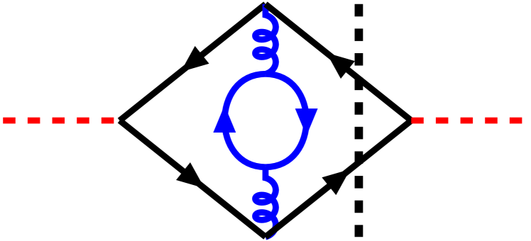
(a)

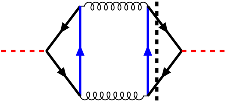
(b)

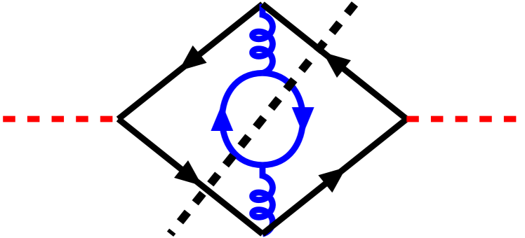
(c)

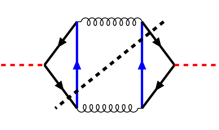
(d)

Figure 8: Typical cut diagrams that have large logarithms $\log^{i}(z)$. The thick black and red lines stand for the massive bottom quark and the Higgs boson, respectively. And the blue line represents the particle that is soft.

These logarithms $\log^{i}(z)$ arise from the diagrams with a bottom quark loop, e.g., see the diagram (a) in figure 8. These diagrams contain up to $1/\epsilon^{3}$ infrared divergences in the massless case, which are converted to $\log^{i}(z),i\leq 3$, in the massive bottom quark case.

It is interesting to note the $\log^{4}(z)$ term at order $\mathcal{O}(z^{-1})$. It appears due to a different reason. It comes from the contribution of diagrams with two soft quarks exchanged between two separate directions, e.g., see the diagram (b) in figure 8.

The other NNLO coefficient $X_{2,b\bar{b}b\bar{b}}^{y_{b}y_{b}}$ consists of master integrals that depend on elliptic integrals. We present the asymptotic expansion results of the master integrals in appendix B. Based on these results, we obtain the asymptotic expansion,

$$X_{2,b\bar{b}b\bar{b}}^{y_{b}y_{b}}|_{z\rightarrow\infty}=\frac{\log^{3}(z)}{27}-\frac{19\log^{2}(z)}{54}-\frac{2\zeta(3)\log(z)}{9}-\frac{\pi^{2}\log(z)}{54}+\frac{503\log(z)}{324}$$

$$\quad+\frac{19\pi^{4}}{1620}-\frac{2\log(2)\pi^{2}}{9}+\frac{5\zeta(3)}{18}+\frac{31\pi^{2}}{108}-\frac{2491}{648}$$

$$\quad+\frac{1}{z}\bigg{(}\frac{\log^{4}(z)}{18}-\frac{\log^{3}(z)}{18}-\frac{2\pi^{2}\log^{2}(z)}{9}+\frac{7\pi^{2}\log(z)}{54}-\frac{\log^{2}(z)}{3}+4\zeta(3)\log(z)$$

$$\quad+\frac{211\log(z)}{54}+\frac{13\pi^{4}}{270}-\frac{7\zeta(3)}{9}+\frac{19\pi^{2}}{18}-\frac{8353}{324}\bigg{)}+\mathcal{O}(z^{-2})\,.$$ (36)

It can be seen that $X_{2,b\bar{b}b\bar{b}}^{y_{b}y_{b}}$ also have large logarithms when $z\rightarrow\infty$. The logarithms $\log^{i}(z),i\leq 3,$ at $\mathcal{O}(z^{0})$ are obtained by calculating the diagrams with a soft gluon splitting to a soft bottom quark pair; see diagram (c) in figure 8. In contrast, the logarithm $\log^{4}(z)$ at $\mathcal{O}(z^{-1})$ arises from the diagrams with a collinear quark splitting to a soft quark and a collinear gluon which splits into a collinear quark and a soft quark further, such as the diagram (d) in figure 8.

Combining the results in eq.(35) and eq.(36), we obtain

$$X_{2}^{y_{b}y_{b}}|_{z\rightarrow\infty\,(m_{b}^{2}\rightarrow 0)}=\frac{55-2n_{l}}{12}\log^{2}\left(\frac{\mu^{2}}{m_{H}^{2}}\right)+\frac{307-11n_{l}}{9}\log\left(\frac{\mu^{2}}{m_{H}^{2}}\right)+\frac{(4n_{l}-113)\zeta(3)}{6}$$

$$\quad+\frac{(2n_{l}-55)\pi^{2}}{36}+\frac{10411-390n_{l}}{144}+\frac{1}{z}\bigg{(}-\frac{\log^{4}(z)}{12}-\frac{\pi^{2}\log^{2}(z)}{6}-\frac{(6n_{l}-25)\log^{2}(z)}{6}$$

$$\quad-\frac{(26n_{l}-829)\log(z)}{6}-(2n_{l}-55)\log(z)\log\left(\frac{\mu^{2}}{m_{H}^{2}}\right)-\frac{5(2n_{l}-55)}{6}\log\left(\frac{\mu^{2}}{m_{H}^{2}}\right)-\frac{\pi^{4}}{12}$$

$$\quad+\frac{4\pi^{2}\log(2)}{3}+47\zeta(3)-\frac{(2n_{l}-41)\pi^{2}}{2}+\frac{791-43n_{l}}{9}\bigg{)}+\mathcal{O}(z^{-2})\,.$$ (37)

The large logarithms of $z$ at $\mathcal{O}(z^{0})$ cancel, as expected. However, the large logarithms at $\mathcal{O}(z^{-1})$ survives. The structure of this kind of large logarithm at higher orders in $\alpha_{s}$ is not well understood. It is promising to explore this issue using the effective field theory, which we leave for future study. After adopting the same renormalization scheme, the above expression is consistent with the result in ref. Harlander:1997xa , which was obtained with the method of large momentum expansion.

It is also interesting to investigate the threshold limit of bottom quark pair production, where the coefficients $X_{1}^{y_{b}y_{b}}$ and $X_{2}^{y_{b}y_{b}}$ are expanded in the limit of $m_{H}\rightarrow 2m_{b}$ or $\beta\rightarrow 0$. Expanding the full analytic results, we have

$$X_{1}^{y_{b}y_{b}}|_{\beta\rightarrow 0}=\frac{2\pi^{2}}{3\beta}+4\log(2)+\frac{4}{3}+2\log\left(\frac{\mu^{2}}{m_{H}^{2}}\right)+\frac{2\pi^{2}\beta}{3}+\mathcal{O}\left(\beta^{2}\right),$$ (38)

and

$$X_{2}^{y_{b}y_{b}}|_{\beta\rightarrow 0}=\frac{1}{\beta^{2}}\left(\frac{4\pi^{4}}{27}+\frac{4\pi^{2}}{9}\right)+\frac{1}{\beta}\bigg{(}\frac{\left(339-22n_{l}\right)\pi^{2}}{54}+\frac{22\log(2)\pi^{2}}{9}$$

$$\quad+\frac{\left(2n_{l}-33\right)\pi^{2}\log(\beta)}{9}+\frac{\left(55-2n_{l}\right)\pi^{2}}{18}\log\left(\frac{\mu^{2}}{m_{H}^{2}}\right)\bigg{)}$$

$$\quad+\bigg{(}\frac{8\pi^{4}}{27}+\frac{(139-3n_{l})\pi^{2}}{27}-\frac{100\log(\beta)\pi^{2}}{27}-\frac{130\log(2)\pi^{2}}{27}-\frac{181\zeta(3)}{9}$$

$$\quad+\frac{(55-2n_{l})}{12}\log^{2}\left(\frac{4\mu^{2}}{m_{H}^{2}}\right)+\frac{(57-2n_{l})}{4}\log\left(\frac{\mu^{2}}{m_{H}^{2}}\right)+\frac{(163-6n_{l})\log(2)}{6}$$

$$\quad+\frac{(13993-506n_{l})}{432}\bigg{)}+\beta\bigg{(}\frac{\left(6n_{l}-303\right)\pi^{2}}{162}+\frac{\left(6n_{l}+101\right)\pi^{2}\log(\beta)}{27}$$

$$\quad+\frac{\left(55-2n_{l}\right)\pi^{2}}{18}\log\left(\frac{\mu^{2}}{m_{H}^{2}}\right)+\frac{418\log(2)\pi^{2}}{27}\bigg{)}+\mathcal{O}\left(\beta^{2}\right).$$ (39)

In obtaining the above compact expressions, we have extensively used the relations among MPLs in Henn:2015sem ; Frellesvig:2016ske . We check that the coefficients of $1/\beta^{2}$ and $1/\beta$ are consistent with the results of two-loop form factors Ablinger:2017hst , which means that the power divergences at $\beta\to 0$ in $X_{1}^{y_{b}y_{b}}$ and $X_{2}^{y_{b}y_{b}}$ come only from virtual corrections. Actually, these velocity-enhanced terms are due to the Coulomb potential interaction between the bottom quark pair. They violate the convergence of perturbative expansion and need to be resummed to all orders in $\alpha_{s}$ by calculating the corresponding Coulomb Green function Beneke:1999qg . Notice that the coefficients of $\pi^{2}/\beta$ in $X_{1}^{y_{b}y_{b}}$ and $\pi^{4}/\beta^{2}$ in $X_{2}^{y_{b}y_{b}}$ agree with those in $e^{+}e^{-}\to t\bar{t}$ production near threshold Czarnecki:1997vz , but the $\pi^{2}/\beta^{2}$ term is different. They can be reproduced by calculating the imaginary part of the first a few terms of the zero-distance Coulomb Green function,

$${\rm Im}~{}G_{0}(E) ={\rm Im}\int\frac{d^{D-1}{\bf{p}}_{1}}{(2\pi)^{D-1}}\frac{{\bf{p}}_{1}\cdot{\bf{p}}_{1}}{E-\frac{{\bf{p}}_{1}^{2}}{m_{b}}}\,+{\rm Im}\int\frac{d^{D-1}{\bf{p}}_{1}}{(2\pi)^{D-1}}\frac{d^{D-1}{\bf{p}}_{2}}{(2\pi)^{D-1}}\frac{{\bf{p}}_{1}\cdot{\bf{p}}_{2}}{E-\frac{{\bf{p}}_{1}^{2}}{m_{b}}}\,\frac{g_{s}^{2}C_{F}}{({\bf{p}}_{1}-{\bf{p}}_{2})^{2}}\,\frac{1}{E-\frac{{\bf{p}}_{2}^{2}}{m_{b}}}$$

$$+{\rm Im}\int\frac{d^{3}{\bf{p}}_{1}}{(2\pi)^{3}}\frac{d^{3}{\bf{p}}_{2}}{(2\pi)^{3}}\frac{d^{3}{\bf{p}}_{3}}{(2\pi)^{3}}\frac{{\bf{p}}_{1}\cdot{\bf{p}}_{3}}{E-\frac{{\bf{p}}_{1}^{2}}{m_{b}}}\,\frac{g_{s}^{2}C_{F}}{({\bf{p}}_{1}-{\bf{p}}_{2})^{2}}\,\frac{1}{E-\frac{{\bf{p}}_{2}^{2}}{m_{b}}}\frac{g_{s}^{2}C_{F}}{({\bf{p}}_{2}-{\bf{p}}_{3})^{2}}\,\frac{1}{E-\frac{{\bf{p}}_{3}^{2}}{m_{b}}}+\mathcal{O}(g_{s}^{6})$$

$$=\frac{\beta^{3}m_{b}^{4}}{4\pi}\left(1+\frac{\alpha_{s}C_{F}}{\pi}\frac{\pi^{2}}{2\beta}+\left(\frac{\alpha_{s}C_{F}}{\pi}\right)^{2}\left(\frac{\pi^{4}}{12\beta^{2}}+\frac{\pi^{2}}{4\beta^{2}}\right)+\mathcal{O}(\alpha_{s}^{3})\right)$$ (40)

with $E=m_{b}\beta^{2}+\mathcal{O}(\beta^{4})$. The ${\bf{p}}_{i}\cdot{\bf{p}}_{j}$ numerator arises because the scalar current $\bar{\psi}_{b}\psi_{b}$ with $\psi_{b}$ the bottom quark field matches to the current $j^{(s)}=\psi^{\dagger}\bm{\sigma}\cdot i{\bf{D}}\chi/m_{b}$ in non-relativistic QCD where $\psi$ and $\chi$ represent the two-component quark and anti-quark field, respectively.

6 Numerical results

We adopt the SM input parameters ParticleDataGroup:2022pth

$$\overline{m_{b}}\,(\overline{m_{b}}) =4.18~{}{\rm GeV}, m_{b} =5.07~{}{\rm GeV},$$

$$m_{H} =125.09~{}{\rm GeV}, m_{Z} =91.1876~{}{\rm GeV},$$ (41)

$$\alpha_{s}(m_{Z}) =0.1181, G_{F} =1.166378\times 10^{-5}~{}{\rm GeV}^{-2},$$

where the on-shell value of $m_{b}$ is obtained from $\overline{m_{b}}(\overline{m_{b}})$ in the $\overline{\rm MS}$ scheme with the four-loop mass relation. The package RunDec Chetyrkin:2000yt ; Herren:2017osy was used to obtain $\overline{m_{b}}$ at other scales, e.g., $\overline{m_{b}}\,(m_{H}/2)=2.956$ GeV, $\overline{m_{b}}\,(m_{H})=2.784$ GeV and $\overline{m_{b}}\,(2m_{H})=2.639$ GeV.

$\quad\quad\mu$	$\quad\frac{1}{2}m_{H}$	$\quad m_{H}$	$\quad 2m_{H}$
$X_{1}^{y_{b}y_{b}}$(our res.)	$+3.037513882$	$+5.810102605$	$+8.582691327$
$X_{1}^{y_{b}y_{b}}$(Ref. Harlander:1997xa )	$+3.037513882$	$+5.810102605$	$+8.582691327$
$\tilde{X}_{2,b\bar{b}}^{y_{b}y_{b}}$(our res.)	$-4.537634223$	$+29.22467780$	$+78.04118427$
${X}_{2}^{y_{b}y_{b}}$(our res.)	$-3.181291730$	$+30.58102030$	$+79.39752676$
${X}_{2}^{y_{b}y_{b}}$(Ref. Harlander:1997xa )	$-3.181291730$	$+30.58102030$	$+79.39752676$

Table 1: The numerical results for the $X_{1}^{y_{b}y_{b}}$, $\tilde{X}_{2}^{y_{b}y_{b}}$ and ${X}_{2}^{y_{b}y_{b}}$ coefficients.

The numerical results of $X_{1}^{y_{b}y_{b}}$ and ${X}_{2}^{y_{b}y_{b}}$ at the scale $\mu=m_{H}/2,m_{H},2m_{H}$ are shown in table 1. We also provide the results from the asymptotic expansion expression in Harlander:1997xa . Perfect agreements were found for both the NLO $X_{1}^{y_{b}y_{b}}$ and NNLO $X_{2}^{y_{b}y_{b}}$ coefficients.

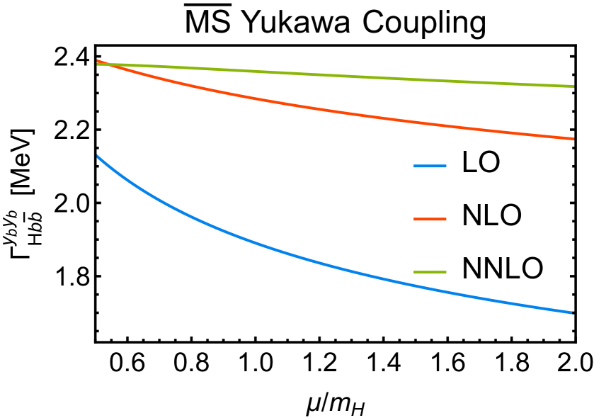
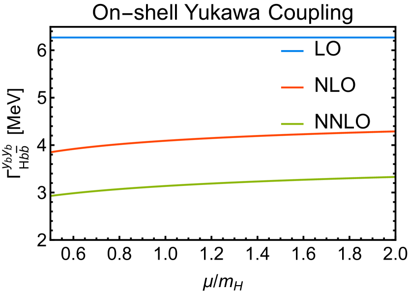
Figure 9: $\Gamma_{Hb\bar{b}}^{y_{b}y_{b}}$ at different values of $\mu$. The left (right) plot corresponds to the result with $\overline{\rm MS}$ (on-shell) Yukawa couplings. The LO, NLO and NNLO predictions are represented by the blue, red, and green lines, respectively.

Combining the corrections up to $\mathcal{O}(y_{b}^{2}\alpha_{s}^{2})$, we obtain $\Gamma^{y_{b}y_{b}}_{Hb\bar{b}}$ up to NNLO. We show the results of $\Gamma^{y_{b}y_{b}}_{Hb\bar{b}}$ with both the $\overline{\rm MS}$ and the on-shell Yukawa coupling in figure 9. The renormalization scale $\mu$ varies from $\mu=1/2m_{H}$ to $\mu=2m_{H}$. In the $\overline{\rm MS}$ scheme, the LO decay width exhibits a strong scale dependence, and it changes by about $23\%$ for $\mu$ in the range $[1/2m_{H},2m_{H}]$. The scale uncertainty is significantly reduced down to about $9\%$ and $3\%$ at NLO and NNLO, respectively. The NLO correction increases the LO decay width by a factor of $12\%\sim 28\%$ depending on the scale. The NNLO correction is very small at $\mu=m_{H}/2$ but can be as large as $7\%$ at $\mu=2m_{H}$.

The LO decay width in the on-shell scheme does not depend on the scale. The scale uncertainty is about $11\%$ and $13\%$ at NLO and NNLO, respectively. At a typical scale $\mu=m_{H}$, the NLO correction decreases the LO result by $35\%$, and the NNLO correction reduces the decay width further by $23\%$. This behavior indicates that the perturbative expansion with the on-shell Yukawa coupling converges slower than that with the $\overline{\rm MS}$ Yukawa coupling.

Comparing the two schemes, one can find that the results in the on-shell scheme are larger than those in the $\overline{\rm MS}$ scheme. The main reason is that the pole mass $m_{b}$ = 5.07 GeV is much larger than the $\overline{\rm MS}$ mass $\overline{m_{b}}(\mu=m_{H})$ = 2.78 GeV. However, higher-order corrections reduce the difference between the two schemes prominently, signifying its importance in providing reliable theoretical predictions.

width	LO	NLO	NNLO($y_{b}^{2}$)	NNLO($y_{b}y_{t}$)	NNNLO($y_{b}^{2}$)	NNNNLO($y_{b}^{2}$)
$\overline{\rm MS}$	1.891${}^{+0.241}_{-0.192}$	2.285${}^{+0.105}_{-0.110}$	2.359${}^{+0.020}_{-0.041}$	2.376${}^{+0.026}_{-0.046}$	2.379${}^{+0.005}_{-0.015}$	2.377${}^{+0.006}_{-0.006}$
on-shell	6.269	4.092${}^{+0.197}_{-0.242}$	3.138${}^{+0.191}_{-0.210}$	3.193${}^{+0.181}_{-0.197}$	2.804${}^{+0.112}_{-0.096}$	2.649${}^{+0.065}_{-0.049}$

Table 2: Decay width of $\Gamma_{Hb\bar{b}}$ (in MeV) at different orders in QCD. The second row shows the results with the $\overline{\rm MS}$ Yukawa coupling while the third row shows the results with the on-shell Yukawa coupling. The renormalization scale uncertainties around $\mu=m_{H}$ are also shown. The NNLO($y_{b}y_{t}$), NNNLO($y_{b}^{2}$), and NNNNLO($y_{b}^{2}$) results were calculated using the formulas in refs. Larin:1995sq ; Chetyrkin:1996sr ; Baikov:2005rw ; Herzog:2017dtz .

Given that the scheme dependence constitutes the dominant theory uncertainty now, it is necessary to see how it changes as higher orders are taken into account. We adopt the $\mathcal{O}(y_{b}y_{t}\alpha_{s}^{2})$ correction in the expansion of $m_{b}^{2}$/$m_{H}^{2}$ and $m_{H}^{2}$/$m_{t}^{2}$ Larin:1995sq , and the $\mathcal{O}(y_{b}^{2}\alpha_{s}^{3})$ and $\mathcal{O}(y_{b}^{2}\alpha_{s}^{4})$ corrections in the massless bottom quark limit Chetyrkin:1996sr ; Baikov:2005rw ; Herzog:2017dtz . One can see that the central value for the decay width in the $\overline{\rm MS}$ scheme becomes stable quickly and that the scale uncertainty is decreased to $\pm 0.3\%$ after the NNNNLO correction is included. In contrast, the NNNLO correction in the on-shell scheme decreases the NNLO result by $12\%$, and the NNNNLO correction reduces the decay width by $5.5\%$ further. The scale uncertainty is still $2\%$ at NNNNLO. All these features manifest that the results in the on-shell scheme have a bad convergence behavior. It is more appropriate to take the $\overline{\rm MS}$ scheme in this high-energy process.

Our analytic results can also be applied to the decay of heavy scalar particles. If there is a new scalar Higgs with a mass of more than 350 GeV, it can decay to a top quark pair. In this process, we have five massless light quarks and one massive top quark. The decay width $\Gamma_{Ht\bar{t}}$ of $H\to t\bar{t}$ with $m_{t}=172.69$ GeV and different values of $m_{H}$ are shown in figure 10. The NNLO correction increases the NLO result by $3\%\sim 17\%$ at $\mu=m_{H}$ as $m_{H}$ varies from 400 GeV to 1 TeV, and the scale uncertainty reduces from $7\%\sim 13\%$ at NLO to $2\%\sim 8\%$ at NNLO.

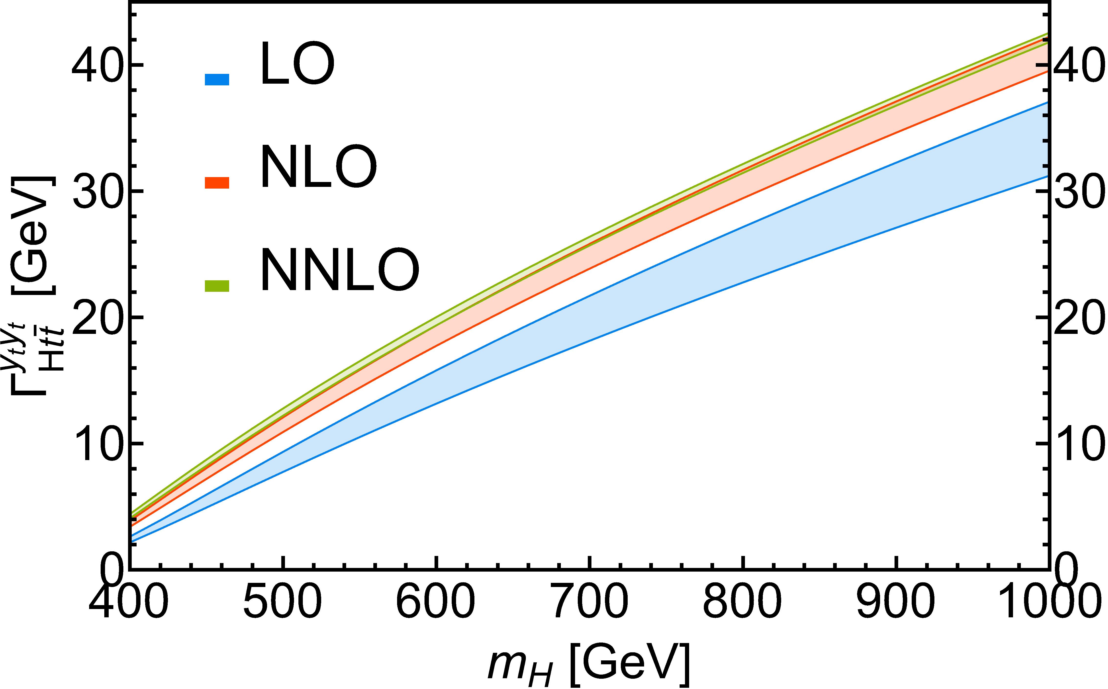
Figure 10: $\Gamma_{Ht\bar{t}}$ at different values of $m_{H}$. The LO, NLO and NNLO predictions with QCD scale uncertainties are represented by the blue, red, and green bands, respectively.

7 Conclusion

We present an exact result of the decay width of $H\to b\bar{b}$ at $\mathcal{O}(y_{b}^{2}\alpha_{s}^{2})$ with full dependence on $m_{b}$. The result is obtained by calculating the imaginary part of the three-loop self-energy diagrams of the Higgs boson which have two bottom quarks in the propagators. The master integrals are calculated using the method of differential equations combined with the choice of a canonical basis. The result has been expressed in terms of multiple polylogarithms. The contribution from the four bottom quarks is also calculated analytically and written as a linear combination of complete elliptic integrals and one-fold integrals of them. The expansion of our analytical result in the small quark mass $m_{b}$ limit agrees with the previous computation in a different method. The threshold expansion shows velocity enhancement which is caused by Coulomb potential interactions. Though the structure is not the same as that in the top quark pair production near the threshold, we checked that the power divergent terms can be reproduced by calculating a new Coulomb Green function. We discuss the numerical results in both the $\overline{\rm MS}$ and on-shell renormalization schemes for the Yukawa coupling. Higher-order QCD corrections reduce both the scale uncertainty and the difference between the two schemes. The analytical results presented in this paper enable accurate and fast evaluation of the decay width of heavy scalar particles.

Appendix A Topologies of the master integrals

The topology diagrams of the master integrals in the NP1 and P1 are displayed below.

$\text{M}^{\text{NP1}}_{1}$

$\text{M}^{\text{NP1}}_{2}$

Appendix B Asymptotic expansion of the master integrals

In the limit of $z\rightarrow\infty\,(m_{b}\rightarrow 0)$, all the master integrals that are needed in $X_{2,b\bar{b}b\bar{b}}^{y_{b}y_{b}}$ can be expanded with the method in Lee:2020obg . Here we present the asymptotic expansion results:

$${F^{4b}_{1}}|_{z\rightarrow\infty}=12\pi\log^{2}(z)-4\pi^{3}$$

$$\quad-\frac{1}{z}\bigg{(}144\pi\log^{2}(z)+144\pi\log(z)-48\pi^{3}\bigg{)}+\mathcal{O}(z^{-2}),$$

$${F^{4b}_{2}}|_{z\rightarrow\infty}=18\pi\log^{2}(z)-24\pi\log(z)-6\pi^{3}$$

$$\quad-\frac{1}{z}\bigg{(}72\pi\log^{2}(z)+72\pi\log(z)-24\pi^{3}-144\pi\bigg{)}+\mathcal{O}(z^{-2}),$$

$${F^{4b}_{3}}|_{z\rightarrow\infty}=-6\pi\log(z)+12\pi$$

$$\quad+\frac{1}{z}\bigg{(}36\pi\log^{2}(z)-36\pi\log(z)-12\pi^{3}+36\pi\bigg{)}+\mathcal{O}(z^{-2}),$$

$${F^{4b}_{4}}|_{z\rightarrow\infty}=12\pi\log^{2}(z)-8\pi^{3}$$

$$\quad-\frac{1}{z}\bigg{(}72\pi\log^{2}(z)+48\pi\log(z)-24\pi^{3}+96\pi\bigg{)}+\mathcal{O}(z^{-2}),$$

$${F^{4b}_{5}}|_{z\rightarrow\infty}=4\pi\log^{3}(z)-4\pi^{3}\log(z)-96\pi\zeta(3)$$

$$\quad+\frac{1}{z}\bigg{(}144\pi\log^{2}(z)+432\pi\log(z)-48\pi^{3}+432\pi\bigg{)}+\mathcal{O}(z^{-2}),$$

$${F^{4b}_{6}}|_{z\rightarrow\infty}=-4\pi\log^{3}(z)+8\pi^{3}\log(z)-36\pi\zeta(3)-8\pi^{3}\log(2)$$

$$\quad-\frac{1}{z}\bigg{(}24\pi\log^{2}(z)+96\pi\log(z)+8\pi^{3}\bigg{)}+\mathcal{O}(z^{-2}),$$

$${F^{4b}_{7}}|_{z\rightarrow\infty}=4\pi\log^{3}(z)-8\pi^{3}\log(z)+72\pi\zeta(3)$$

$$\quad+\frac{1}{z}\bigg{(}48\pi\log^{2}(z)+144\pi\log(z)-8\pi^{3}+48\pi\bigg{)}+\mathcal{O}(z^{-2}),$$

$${F^{4b}_{8}}|_{z\rightarrow\infty}=-2\pi\log^{3}(z)+6\pi^{3}\log(z)-60\pi\zeta(3)-8\pi^{3}\log(2)$$

$$\quad-\frac{1}{z}\bigg{(}12\pi\log^{2}(z)-4\pi^{3}-96\pi\bigg{)}+\mathcal{O}(z^{-2}),$$

$${F^{4b}_{9}}|_{z\rightarrow\infty}=-\frac{1}{2}\pi\log^{4}(z)+\pi^{3}\log^{2}(z)+24\pi\zeta(3)\log(z)-\frac{19\pi^{5}}{10}$$

$$\quad+\frac{1}{z}\bigg{(}4\pi\log^{3}(z)+24\pi\log^{2}(z)-4\pi^{3}\log(z)+144\pi\log(z)-48\pi\zeta(3)+8\pi^{3}+240\pi\bigg{)}$$

$$\quad+\mathcal{O}(z^{-2}),$$

$${F^{4b}_{10}}|_{z\rightarrow\infty}=\pi\log^{4}(z)-4\pi^{3}\log^{2}(z)+72\pi\zeta(3)\log(z)+\frac{13\pi^{5}}{15}$$

$$\quad-\frac{1}{z}\bigg{(}48\pi\log^{2}(z)+240\pi\log(z)-8\pi^{3}+288\pi\bigg{)}+\mathcal{O}(z^{-2}),$$

$${F^{4b}_{12}}|_{z\rightarrow\infty}=\frac{3}{4}\pi\log^{4}(z)-\frac{7}{2}\pi^{3}\log^{2}(z)+96\pi\zeta(3)\log(z)-\frac{43\pi^{5}}{60}$$

$$\quad-\frac{1}{z}\bigg{(}6\pi\log^{3}(z)+30\pi\log^{2}(z)-14\pi^{3}\log(z)+96\pi\log(z)+192\pi\zeta(3)-10\pi^{3}+36\pi\bigg{)}$$

$$\quad+\mathcal{O}(z^{-2}).$$ (42)

References

- (1) ATLAS collaboration, A detailed map of Higgs boson interactions by the ATLAS experiment ten years after the discovery, Nature 607 (2022) 52–59, [2207.00092].
- (2) CMS collaboration, A. Tumasyan et al., A portrait of the Higgs boson by the CMS experiment ten years after the discovery, Nature 607 (2022) 60–68, [2207.00043].
- (3) Particle Data Group collaboration, R. L. Workman et al., Review of Particle Physics, PTEP 2022 (2022) 083C01.
- (4) CMS collaboration, A. M. Sirunyan et al., Measurement of the top quark Yukawa coupling from kinematic distributions in the lepton+jets final state in proton-proton collisions at 13 TeV, Phys. Rev. D 100 (2019) 072007, [1907.01590].
- (5) CMS collaboration, A. M. Sirunyan et al., Measurement of the top quark Yukawa coupling from kinematic distributions in the dilepton final state in proton-proton collisions at 13 TeV, Phys. Rev. D 102 (2020) 092013, [2009.07123].
- (6) ATLAS collaboration, M. Aaboud et al., Observation of decays and production with the ATLAS detector, Phys. Lett. B 786 (2018) 59–86, [1808.08238].
- (7) CMS collaboration, A. M. Sirunyan et al., Observation of Higgs boson decay to bottom quarks, Phys. Rev. Lett. 121 (2018) 121801, [1808.08242].
- (8) ATLAS collaboration, G. Aad et al., Direct constraint on the Higgs-charm coupling from a search for Higgs boson decays into charm quarks with the ATLAS detector, Eur. Phys. J. C 82 (2022) 717, [2201.11428].
- (9) CMS collaboration, A. Tumasyan et al., Search for Higgs Boson Decay to a Charm Quark-Antiquark Pair in Proton-Proton Collisions at s=13 TeV, Phys. Rev. Lett. 131 (2023) 061801, [2205.05550].
- (10) ATLAS collaboration, G. Aad et al., Measurements of Higgs boson production cross-sections in the decay channel in pp collisions at = 13 TeV with the ATLAS detector, JHEP 08 (2022) 175, [2201.08269].
- (11) CMS collaboration, A. Tumasyan et al., Measurements of Higgs boson production in the decay channel with a pair of leptons in proton–proton collisions at TeV, Eur. Phys. J. C 83 (2023) 562, [2204.12957].
- (12) ATLAS collaboration, G. Aad et al., A search for the dimuon decay of the Standard Model Higgs boson with the ATLAS detector, Phys. Lett. B 812 (2021) 135980, [2007.07830].
- (13) CMS collaboration, A. M. Sirunyan et al., Evidence for Higgs boson decay to a pair of muons, JHEP 01 (2021) 148, [2009.04363].
- (14) F. An et al., Precision Higgs physics at the CEPC, Chin. Phys. C 43 (2019) 043002, [1810.09037].
- (15) CEPC Physics Study Group collaboration, H. Cheng et al., The Physics potential of the CEPC. Prepared for the US Snowmass Community Planning Exercise (Snowmass 2021), in Snowmass 2021, 5, 2022, 2205.08553.
- (16) Y. Zhu, H. Cui and M. Ruan, The Higgs→,, gg measurement at CEPC, JHEP 11 (2022) 100, [2203.01469].
- (17) E. Braaten and J. P. Leveille, Higgs Boson Decay and the Running Mass, Phys. Rev. D 22 (1980) 715.
- (18) N. Sakai, Perturbative QCD Corrections to the Hadronic Decay Width of the Higgs Boson, Phys. Rev. D 22 (1980) 2220.
- (19) P. Janot, First Order QED and QCD Radiative Corrections to Higgs Decay Into Massive Fermions, Phys. Lett. B 223 (1989) 110–118.
- (20) M. Drees and K.-i. Hikasa, NOTE ON QCD CORRECTIONS TO HADRONIC HIGGS DECAY, Phys. Lett. B 240 (1990) 455.
- (21) A. Dabelstein and W. Hollik, Electroweak corrections to the fermionic decay width of the standard Higgs boson, Z. Phys. C 53 (1992) 507–516.
- (22) B. A. Kniehl, Radiative corrections for f anti-f () in the standard model, Nucl. Phys. B 376 (1992) 3–28.
- (23) A. L. Kataev, The Order O (alpha alpha-s) and O (alpha**2) corrections to the decay width of the neutral Higgs boson to the anti-b b pair, JETP Lett. 66 (1997) 327–330, [hep-ph/9708292].
- (24) L. Mihaila, B. Schmidt and M. Steinhauser, to order , Phys. Lett. B 751 (2015) 442–447, [1509.02294].
- (25) S. G. Gorishnii, A. L. Kataev, S. A. Larin and L. R. Surguladze, Corrected Three Loop QCD Correction to the Correlator of the Quark Scalar Currents and (Tot) ( Hadrons), Mod. Phys. Lett. A 5 (1990) 2703–2712.
- (26) K. G. Chetyrkin, Correlator of the quark scalar currents and Gamma(tot) (H — hadrons) at O (alpha-s**3) in pQCD, Phys. Lett. B 390 (1997) 309–317, [hep-ph/9608318].
- (27) P. A. Baikov, K. G. Chetyrkin and J. H. Kuhn, Scalar correlator at O(alpha(s)**4), Higgs decay into b-quarks and bounds on the light quark masses, Phys. Rev. Lett. 96 (2006) 012003, [hep-ph/0511063].
- (28) F. Herzog, B. Ruijl, T. Ueda, J. A. M. Vermaseren and A. Vogt, On Higgs decays to hadrons and the R-ratio at N4LO, JHEP 08 (2017) 113, [1707.01044].
- (29) R. Mondini, M. Schiavi and C. Williams, N3LO predictions for the decay of the Higgs boson to bottom quarks, JHEP 06 (2019) 079, [1904.08960].
- (30) X. Chen, P. Jakubčík, M. Marcoli and G. Stagnitto, The parton-level structure of Higgs decays to hadrons at N3LO, JHEP 06 (2023) 185, [2304.11180].
- (31) W. Bernreuther, L. Chen and Z.-G. Si, Differential decay rates of CP-even and CP-odd Higgs bosons to top and bottom quarks at NNLO QCD, JHEP 07 (2018) 159, [1805.06658].
- (32) A. Behring and W. Bizoń, Higgs decay into massive b-quarks at NNLO QCD in the nested soft-collinear subtraction scheme, JHEP 01 (2020) 189, [1911.11524].
- (33) G. Somogyi and F. Tramontano, Fully exclusive heavy quark-antiquark pair production from a colourless initial state at NNLO in QCD, JHEP 11 (2020) 142, [2007.15015].
- (34) W. Bizoń, E. Re and G. Zanderighi, NNLOPS description of the decay with MiNLO, JHEP 06 (2020) 006, [1912.09982].
- (35) Y. Hu, C. Sun, X.-M. Shen and J. Gao, Hadronic decays of Higgs boson at NNLO matched with parton shower, JHEP 08 (2021) 122, [2101.08916].
- (36) R. Mondini and C. Williams, at next-to-next-to-leading order accuracy, JHEP 06 (2019) 120, [1904.08961].
- (37) J. Gao, Higgs boson decay into four bottom quarks in the SM and beyond, JHEP 08 (2019) 174, [1905.04865].
- (38) A. Primo, G. Sasso, G. Somogyi and F. Tramontano, Exact Top Yukawa corrections to Higgs boson decay into bottom quarks, Phys. Rev. D 99 (2019) 054013, [1812.07811].
- (39) R. Mondini, U. Schubert and C. Williams, Top-induced contributions to and at , JHEP 12 (2020) 058, [2006.03563].
- (40) K. G. Chetyrkin and A. Kwiatkowski, Second order QCD corrections to scalar and pseudoscalar Higgs decays into massive bottom quarks, Nucl. Phys. B 461 (1996) 3–18, [hep-ph/9505358].
- (41) R. Harlander and M. Steinhauser, Higgs decay to top quarks at O (alpha-s**2), Phys. Rev. D 56 (1997) 3980–3990, [hep-ph/9704436].
- (42) T. Hahn, Generating Feynman diagrams and amplitudes with FeynArts 3, Comput. Phys. Commun. 140 (2001) 418–431, [hep-ph/0012260].
- (43) V. Shtabovenko, R. Mertig and F. Orellana, FeynCalc 9.3: New features and improvements, Comput. Phys. Commun. 256 (2020) 107478, [2001.04407].
- (44) F. V. Tkachov, A Theorem on Analytical Calculability of Four Loop Renormalization Group Functions, Phys. Lett. B 100 (1981) 65–68.
- (45) K. G. Chetyrkin and F. V. Tkachov, Integration by Parts: The Algorithm to Calculate beta Functions in 4 Loops, Nucl. Phys. B 192 (1981) 159–204.
- (46) S. Laporta, High precision calculation of multiloop Feynman integrals by difference equations, Int. J. Mod. Phys. A 15 (2000) 5087–5159, [hep-ph/0102033].
- (47) A. V. Smirnov and F. S. Chuharev, FIRE6: Feynman Integral REduction with Modular Arithmetic, Comput. Phys. Commun. 247 (2020) 106877, [1901.07808].
- (48) J. Klappert, F. Lange, P. Maierhöfer and J. Usovitsch, Integral reduction with Kira 2.0 and finite field methods, Comput. Phys. Commun. 266 (2021) 108024, [2008.06494].
- (49) R. N. Lee and A. I. Onishchenko, -regular basis for non-polylogarithmic multiloop integrals and total cross section of the process , JHEP 12 (2019) 084, [1909.07710].
- (50) A. V. Kotikov, Differential equations method: New technique for massive Feynman diagrams calculation, Phys. Lett. B 254 (1991) 158–164.
- (51) A. V. Kotikov, Differential equation method: The Calculation of N point Feynman diagrams, Phys. Lett. B 267 (1991) 123–127.
- (52) J. M. Henn, Multiloop integrals in dimensional regularization made simple, Phys. Rev. Lett. 110 (2013) 251601, [1304.1806].
- (53) A. B. Goncharov, Multiple polylogarithms, cyclotomy and modular complexes, Math. Res. Lett. 5 (1998) 497–516, [1105.2076].
- (54) M. Argeri, S. Di Vita, P. Mastrolia, E. Mirabella, J. Schlenk, U. Schubert et al., Magnus and Dyson Series for Master Integrals, JHEP 03 (2014) 082, [1401.2979].
- (55) L.-B. Chen and J. Wang, Analytic two-loop master integrals for tW production at hadron colliders: I *, Chin. Phys. C 45 (2021) 123106, [2106.12093].
- (56) C. Duhr and F. Dulat, PolyLogTools — polylogs for the masses, JHEP 08 (2019) 135, [1904.07279].
- (57) J. Vollinga and S. Weinzierl, Numerical evaluation of multiple polylogarithms, Comput. Phys. Commun. 167 (2005) 177, [hep-ph/0410259].
- (58) C. W. Bauer, A. Frink and R. Kreckel, Introduction to the GiNaC framework for symbolic computation within the C++ programming language, J. Symb. Comput. 33 (2002) 1–12, [cs/0004015].
- (59) X. Liu, Y.-Q. Ma and C.-Y. Wang, A Systematic and Efficient Method to Compute Multi-loop Master Integrals, Phys. Lett. B 779 (2018) 353–357, [1711.09572].
- (60) X. Liu, Y.-Q. Ma, W. Tao and P. Zhang, Calculation of Feynman loop integration and phase-space integration via auxiliary mass flow, Chin. Phys. C 45 (2021) 013115, [2009.07987].
- (61) X. Liu and Y.-Q. Ma, AMFlow: A Mathematica package for Feynman integrals computation via auxiliary mass flow, Comput. Phys. Commun. 283 (2023) 108565, [2201.11669].
- (62) H. Ferguson and D. Bailey, A polynomial time, numerically stable integer relation algorithm, 1992.
- (63) H. Ferguson, D. Beiley and S. Arno, Analysis of PSLQ, an integer relation finding algorithm, Math. Comp. 68 (1999) 351.
- (64) W. E. Caswell, Asymptotic Behavior of Nonabelian Gauge Theories to Two Loop Order, Phys. Rev. Lett. 33 (1974) 244.
- (65) D. R. T. Jones, Two Loop Diagrams in Yang-Mills Theory, Nucl. Phys. B 75 (1974) 531.
- (66) M. Czakon, A. Mitov and S. Moch, Heavy-quark production in gluon fusion at two loops in QCD, Nucl. Phys. B 798 (2008) 210–250, [0707.4139].
- (67) K. Melnikov and T. v. Ritbergen, The Three loop relation between the MS-bar and the pole quark masses, Phys. Lett. B 482 (2000) 99–108, [hep-ph/9912391].
- (68) D. J. Broadhurst, N. Gray and K. Schilcher, Gauge invariant on-shell Z(2) in QED, QCD and the effective field theory of a static quark, Z. Phys. C 52 (1991) 111–122.
- (69) N. Gray, D. J. Broadhurst, W. Grafe and K. Schilcher, Three Loop Relation of Quark (Modified) Ms and Pole Masses, Z. Phys. C 48 (1990) 673–680.
- (70) P. Marquard, A. V. Smirnov, V. A. Smirnov and M. Steinhauser, Quark Mass Relations to Four-Loop Order in Perturbative QCD, Phys. Rev. Lett. 114 (2015) 142002, [1502.01030].
- (71) P. Marquard, A. V. Smirnov, V. A. Smirnov, M. Steinhauser and D. Wellmann, -on-shell quark mass relation up to four loops in QCD and a general SU gauge group, Phys. Rev. D 94 (2016) 074025, [1606.06754].
- (72) T. Kinoshita, Mass singularities of Feynman amplitudes, J. Math. Phys. 3 (1962) 650–677.
- (73) T. D. Lee and M. Nauenberg, Degenerate Systems and Mass Singularities, Phys. Rev. 133 (1964) B1549–B1562.
- (74) J. M. Henn, A. V. Smirnov and V. A. Smirnov, Evaluating Multiple Polylogarithm Values at Sixth Roots of Unity up to Weight Six, Nucl. Phys. B 919 (2017) 315–324, [1512.08389].
- (75) H. Frellesvig, D. Tommasini and C. Wever, On the reduction of generalized polylogarithms to and and on the evaluation thereof, JHEP 03 (2016) 189, [1601.02649].
- (76) J. Ablinger, A. Behring, J. Blümlein, G. Falcioni, A. De Freitas, P. Marquard et al., Heavy quark form factors at two loops, Phys. Rev. D 97 (2018) 094022, [1712.09889].
- (77) M. Beneke, A. Signer and V. A. Smirnov, Top quark production near threshold and the top quark mass, Phys. Lett. B 454 (1999) 137–146, [hep-ph/9903260].
- (78) A. Czarnecki and K. Melnikov, Two loop QCD corrections to the heavy quark pair production cross-section in e+ e- annihilation near the threshold, Phys. Rev. Lett. 80 (1998) 2531–2534, [hep-ph/9712222].
- (79) K. G. Chetyrkin, J. H. Kuhn and M. Steinhauser, RunDec: A Mathematica package for running and decoupling of the strong coupling and quark masses, Comput. Phys. Commun. 133 (2000) 43–65, [hep-ph/0004189].
- (80) F. Herren and M. Steinhauser, Version 3 of RunDec and CRunDec, Comput. Phys. Commun. 224 (2018) 333–345, [1703.03751].
- (81) S. A. Larin, T. van Ritbergen and J. A. M. Vermaseren, The Large top quark mass expansion for Higgs boson decays into bottom quarks and into gluons, Phys. Lett. B 362 (1995) 134–140, [hep-ph/9506465].
- (82) J. Ellis, TikZ-Feynman: Feynman diagrams with TikZ, Comput. Phys. Commun. 210 (2017) 103–123, [1601.05437].
- (83) R. N. Lee, A. A. Lyubyakin and V. A. Stotsky, Total cross sections of processes with via multiloop methods, JHEP 01 (2021) 144, [2010.15430].