Navigating the Complex Landscape of Shock Filter Cahn-Hilliard Equation: From Regularized to Young Measure Solutions

Abstract

Image inpainting involves filling in damaged or missing regions of an image by utilizing information from the surrounding areas. In this paper, we investigate a highly nonlinear partial differential equation inspired by the modified Cahn-Hilliard equation. Instead of using standard potentials that depend solely on pixel intensities, we consider morphological image enhancement filters that are based on a variant of the shock filter:

$$\partial_{t}u =\Delta\left(-\nu\left(\arctan(\Delta u)|\nabla u|\right)-\mu\Delta u\right)+\lambda(u_{0}-u).$$

This is referred to as the Shock Filter Cahn-Hilliard Equation. This equation is nonlinear with respect to the second-order derivative, which poses significant mathematical challenges. To address these, we make use of a specific approximation argument, establishing the existence of a family of approximate solutions through the Leray-Schauder fixed point theorem and the Aubin-Lions lemma. In the limit, we obtain a solution strategy wherein we can prove the existence and uniqueness of solutions. Proving the latter involves the use of Young measures and Kruzhkov entropy type-admissibility conditions.

Additionally, we use a numerical method based on the convexity splitting idea to approximate solutions of the nonlinear partial differential equation and achieve fast inpainting results. To demonstrate the effectiveness of our approach, we apply our method to standard binary images and compare it with variations of the Cahn-Hilliard equation commonly used in the field.

MSC Classification]65M06, 94A08, 68U10, 47H10, 35K55, 80A22

1 Introduction

Digital image inpainting is an important task in image processing applications that involves reconstructing unknown regions of an image based on information from its surrounding areas. We will refer to these unknown regions as the inpainting domain. For a given image $u_{0}$, defined on the image domain $\Omega\subset\mathbb{R}^{2}$, the objective is to restore the image on the inpainting domain $\omega\subset\Omega$ so that the reconstructions are not easily detectable by an ordinary observer.

Drawing inspiration from the manual inpainting techniques, Bertalmio et al. [2] were among the first to introduce an anisotropic PDE that smoothly propagates information from outside the inpainting domain $\Omega\setminus\omega$ inside the domain, following the direction of isophotes (contours of constant greyscale intensity). In particular, anisotropic diffusion is a natural choice as it ensures the sharpness of the reconstructed image. Furthermore, they incorporated the isophote direction as a boundary condition at the edges of the inpainting domain. More precisely, this means that

$$u_{t}=-\nabla^{\perp}u\cdot\nabla\Delta u,$$ (1.1)

had to be solved on $\omega$, where the perpendicular gradient $\nabla^{\perp}u=(-u_{y},u_{x})$ is the direction of smallest change in the image intensity and $\Delta u$ is the measure of image smoothness. Because isophotes depend on the geometry of the inpainting domain and can intersect at the final time, it became necessary to intertwine this process with a diffusion procedure.

As discussed in [3], this approach borrows ideas from computational fluid dynamics and applies them to image analysis challenges. To make it more apparent, one can visualize image intensity as a stream function for a two-dimensional incompressible flow. In this analogy, the Laplacian of the image intensity acts as the fluid’s vorticity and is transported into the inpainting domain by a vector field defined by the stream function. Such an interpretation underscores the need for incorporating diffusion into the inpainting problem. Finally, this approach is designed to preserve isophotes while ensuring that the gradient vectors match at the boundary of the inpainting domain. This method is based on the Navier-Stokes equations of fluid dynamics, taking advantage of well-established theoretical and numerical results in that field.

Because the success of the inpainting process depends on the preferences of the human observer, perception of edges, color, and texture, it is reasonable to model the missing edges using elastica-type curves [57, 63, 54].

More precisely, if we extend the inpainting domain $\omega$ in $\Omega$ and denote it by $\omega_{\epsilon}$, then we can extrapolate the isophotes of an image $u$ by a collection of curves $\{\gamma_{t}\}_{t\in[I_{0},I_{m}]}$ with no mutual crossing, which coincides with the isophotes of $u$ on $\omega_{\epsilon}\setminus\omega$ and minimize the energy

$$\int_{I_{0}}^{I_{m}}\!\!\int_{\gamma_{t}}(\alpha+\beta|\kappa_{\gamma_{t}}|^{p})dsdt,$$ (1.2)

where $[I_{0},I_{M}]$ is the intensity span and $\kappa_{\gamma_{t}}$ is the curvature of $\gamma_{t}$. By adjusting parameters $\alpha$ and $\beta$ based on the specific application at hand, this energy effectively penalizes a generalized form of Euler’s elastica energy.

In [57], the authors introduced two inpainting models. The first is based on the seminal Mumford-Shah image model [47], while the second—termed the Mumford-Shah-Euler image model—serves as its high-order correction. This enhanced model augments the original by substituting the embedded straight-line curve model with Euler’s elastica, a concept initially presented by Mumford in the context of curve modeling. Although this approach provides a more refined representation, it comes with a computational cost. Recognizing this challenge, efforts have been directed towards devising more efficient algorithms. To this end, various extensions that employ augmented Lagrangians have been explored, as documented in [13, 62, 68].

This type of model falls in the category of variational inpainting which is an umbrella term that, among others, incorporates the total variation inpainting [56, 31, 20], and the active contour model based on the well-known Mumford and Shah’s segmentation [64]. In particular, Esedoglu and Shen [32] introduced a modification of the Mumford–Shah segmentation model [58, 64] that incorporates curvature of edge contours into the functional. The curvature term provides us with control over both the position and direction of edges in the digital image. More precisely, for a given image $u_{0}(x)$, one needs to minimize

$$MSE(u,K)=\int_{\Omega\setminus K}|\nabla u|^{2}dx+\int_{K}(\alpha+\beta\kappa^{2})ds+\lambda\int_{\Omega\setminus\omega}(u-u_{0})^{2}dx,$$ (1.3)

where the unknown set $K$ represents edge collection i.e. union of curves and approximates the edges of the given image $u_{0}(x)$, $\kappa$ is the curvature, $ds$ the length element, $\lambda$ is a positive constant, and $\alpha$ and $\beta$ are two positive constants as before. The last term in (1.3) is called the fidelity term and it penalizes deviations, in the $L^{2}$ sense, of the piecewise smooth function $u$ from the original image $u_{0}$ outside of the inpainting domain. Several years later Bertozzi et al. [4, 5] proposed a binary image inpainting model that simplifies the previously presented Esedoglu–Shen model (1.3). Moreover, they observed that the fourth-order gradient flow present in the Esedoglu–Shen model shared similarities with a much simpler model called the Cahn–Hilliard equation.

1.1 The Cahn-Hilliard equation

The Cahn-Hilliard equation (also CHE in the sequel) is a macroscopic field model that describes the phase separation [19, 49] of a binary alloy at a fixed temperature. Beyond its primary application, the CHE is used in diverse domains, including pattern formation [67, 69], biology [38], fluid dynamics [43, 40, 44], and most notably in image processing [15, 9, 10, 11, 12]. Let $u_{0}:\Omega\subset\mathbb{R}^{2}\to\{-1,1\}$ be a given binary image, and suppose that $\omega\subset\Omega$ denotes the inpainting domain. The interpolation $u:(0,T)\times\Omega\to\{-1,1\}$ of the original image $u_{0}$ is obtained as the solution of the modified CHE:

$$u_{t} =\Delta\left(-\nu H^{\prime}(u)-\mu\Delta u\right)+\lambda({\bf x})(u_{0}-u),\;\;\text{on}\;\;(0,T)\times\Omega,$$ (1.4)

$$u\big{|}_{t=0} =u_{0}({\bf x}),\ \$$ (1.5)

together with the appropriate boundary conditions that will be discussed later. Here, the constants $\mu,\nu>0$ depend on a concrete situation, and for some large $\lambda_{0}>0$, the fidelity term $\lambda:\Omega\to\mathbb{R}$ is defined as follows

$$\lambda({\bf x})=\begin{cases}\lambda_{0},\;\;\;\text{if }{\bf x}\in\Omega\setminus\omega,\\ 0,\;\;\;\text{if }{\bf x}\in\omega.\end{cases}$$ (1.6)

In the special case when $H(u)=\frac{1}{2}(1-u^{2})^{2}$ (termed the double-well potential), equation (1.4) reduces to the well-known CHE, as detailed in the original paper [16]). Before delving into various forms of $H$, let us briefly comment on the fidelity term $\lambda$.

The fidelity term plays a crucial role in the equation, ensuring that the inpainted image $u$ closely resembles the original image $u_{0}$ outside the damaged areas. Indeed, for large $\lambda_{0}$ the term $\lambda({\bf x})(u-u_{0})$ must not be large or it cannot be controlled by the rest of the equation. Therefore, for large $\lambda_{0}$, the inpainted image $u$ must be close to the original image in the domain $\Omega\backslash\omega$ (since then the product $\lambda_{0}(u-u_{0})$ is moderate and, roughly speaking, can be controlled by $u_{t}-\Delta\left(-\nu H^{\prime}(u)-\mu\Delta u\right)$; see also (1.3)). We note in passing that this is also the reason why the boundary data for (1.4) are not of substantial importance and it will have an influence only in a very small neighborhood of the boundary (assuming that the inpainted domain is away from the boundary). Moreover, the presence of $\lambda$ ensures that the form of the image has no influence on the inpainting away from the inpainting domain and we can always extend the image domain and force boundary conditions of our choice. Let us now discuss choices of $H$.

1.2 The choice of nonlinear potential $H$

The functional $H(u)$ represents a nonlinear potential with two wells corresponding to $u=-1$ and $u=1$. In the context of inpainting binary images, the values $u=1$ and $u=-1$ can signify the white and black pixels, respectively. In short, since $H$ drives the pixel intensities toward one of these wells, one could, borrowing from machine learning terminology, view $H$ as a form of classifier. In the recent literature, the search for the physically meaningful potential $H$ has been extensive. The initial motivation for this arose from a simple observation that the solutions $u$ of the CHE equipped with double-well potential do not stay bounded to the interval $[-1,1]$. In many applications, this violates the inherent physical laws governing the system. However, from a computational standpoint, one can address this issue using thresholding techniques. These methods redefine any values of $u>1$ as $u=1$ and any values of $u<-1$ as $u=-1$. For example, this approach can be found in the research by Cherfils et al. [25], wherein the numerical scheme is paired with thresholding in its final steps.

Another possibility is to utilize the non-smooth logarithmic potentials [26, 27]:

$$H_{log}(u)=\frac{\theta}{2}\left((1+u)\log(1+u)+(1-u)\log(1-u)\right)+\frac{\theta_{c}}{2}(1-u^{2}),$$ (1.7)

where $0<\theta<\theta_{c}$ is a constant. The singularity of $H_{log}^{\prime}(u)$ furthermore imposes the bounds on $u\in(-1,1)$. The application of a non-smooth logarithmic potential in image inpainting tasks has been demonstrated to decrease the convergence time [24].

In recent years, a version of the CHE that uses a non-smooth potential has been studied in works such as [9, 34] for image inpainting problems. This approach involves using a non-smooth double obstacle potential, defined as:

$$H_{quad}(u)=\psi(u)+\frac{1}{2}(1-u)^{2},\;\;\;\;\;\;\psi(u)=I_{[-1,1]}(u)=\begin{cases}0,\;\;\;\text{if }u\in[-1,1],\\ +\infty,\;\;\;\text{otherwise,}\end{cases}$$ (1.8)

where $I_{A}$ is the indicator function of the set $A$. In [9], authors developed an efficient finite-element solver for image inpainting problems and demonstrated that non-smooth potential produces superior results when compared to the double well potential.

At the end of this subsection, we note that a well-posedness result for a more general situation of (1.13) with so-called degenerate diffusion mobility (i.e. the diffusion coefficient depends on $u$ as well) was obtained in [28].

1.3 Numerical solutions based on the convexity splitting approach

An additional noteworthy aspect of this approach is the availability of efficient numerical methods for solving the CHE [9, 21, 6]. Here, we will employ ideas based on the convexity splitting approach introduced by Eyre [33], and later investigated by several researchers in [21, 36, 37, 60]. In the convexity splitting scheme, the energy functionals are divided into a convex and a concave part. The main idea is to treat the convex part implicitly and the concave part explicitly. Namely, let $\mathcal{H}$ be a Hilbert space and $\mathcal{E}=\mathcal{E}_{1}-\mathcal{E}_{2}$ energy such that it could be written as the difference of two convex energies $\mathcal{E}_{1}$ and $\mathcal{E}_{2}$. Then, the discretization

$$\frac{u^{n+1}-u^{n}}{\Delta t}=-\nabla_{\mathcal{H}}\mathcal{E}_{1}(u^{n+1})-\nabla_{\mathcal{H}}\mathcal{E}_{2}(u^{n}),$$ (1.9)

of the gradient flow

$$u_{t}=-\nabla_{\mathcal{H}}\mathcal{E}(u),$$ (1.10)

satisfies the energy stability property $\mathcal{E}(u^{n+1})\leq\mathcal{E}(u^{n})$. Moreover, under the right conditions [1], this approach can allow for an unconditionally stable time-discretization scheme. The CHE is derived as the $H^{-1}$ gradient flow of the Ginzburg–Landau energy defined in the following way:

$$\mathcal{E}_{1}[u]=\int_{\Omega}\left[\nu H(u({\bf x}))+\frac{1}{2}\mu|\nabla u({\bf x})|^{2}\right]d{\bf x},$$ (1.11)

where $u$ typically denotes the concentration, $H(u)$ is the Helmholtz free energy density, $\varepsilon$ is proportional to the thickness of the transition region between two phases. For further insights into the derivation of both first and second-order unconditionally energy-stable numerical schemes based on equation (1.11), the work in [1] serves as a comprehensive reference.

In addition, one could derive the fidelity term as the $L^{2}$ gradient flow of energy defined by

$$\mathcal{E}_{2}[u]=\frac{\lambda}{2}\int_{\Omega\setminus\omega}\left(u_{0}-u\right)^{2}d{\bf x}.$$ (1.12)

Let us note that modified CHE (1.4) is not strictly a gradient flow but could be interpreted as the superposition of gradient descent with respect to $H^{-1}$ inner product for energy defined with (1.11) and the gradient descent with the respect to $L^{2}$ inner product defined with (1.12).

As we will see in Section 4, the numerical method based on convexity splitting can be applied to the modified CHE (1.4) by applying it to functionals $\mathcal{E}_{1}$ and $\mathcal{E}_{2}$ separately.

1.4 The current contribution

Recently, in [48] a regularized version of the shock filters $-\mathop{\rm sgn\,}\nolimits({\Delta u})|\nabla u|$ developed by Rudin and Osher [50] was considered as a potential choice for the generalization of the functional $H$. Here, $-\mathop{\rm sgn\,}\nolimits({\Delta u})$ is an edge-detection term that exhibits a changing sign across any essential singular feature so that the local flow field is governed toward the features, and $|\nabla u|$ is the magnitude of the gradient. The main idea is based on utilizing a dilation process in proximity to image maxima and an erosion process surrounding image minima. To ascertain the influence zone of each maximum and minimum, the Laplacian is employed as a classifier. If the Laplacian is negative, the pixel in question is assigned to the influence zone of a maximum; conversely, if the Laplacian is positive, the pixel is considered to belong to the influence zone of a minimum. When applied to the digital image, this equation creates strong discontinuities at image edges and a piecewise constant segmentation within regions of similar grayscale intensities. Accordingly, iterated shock filtering may be conceived of as a morphological segmentation technique. Shock filter belongs to the class of morphological image enhancement equations [14, 35, 17, 61]. From the mathematical point of view, this equation satisfies a maximum–minimum principle which means that the pixel intensities of the processed image will remain within the range of the original image. Besides the mathematical analysis of the regularized equation, the authors [48] demonstrated that this equation shows the tendency to extend image structures while preserving image sharpness, therefore eliminating the diffusive effects visible in the case of a CHE with a double-well potential. However, in certain examples, this modification of CHE has demonstrated an uncritical tendency to form edges, and additional steps are needed to control this effect. In this paper, we will address this issue by proposing a more regular classifier $-|\nabla u|\arctan({\Delta u})$ that, in applications, has a less expressed tendency towards edge formation. The problem to be considered here thus has the form

$$\partial_{t}u =\Delta\Big{(}-\nu\arctan(\Delta u)|\nabla u|-\mu\Delta u\Big{)}+\lambda(u_{0}-u)\;\;\text{on}\;\;(0,T)\times\Omega,$$ (1.13)

$$u(t,{\bf x}) =u_{0}({\bf x})\;\;\text{on}\;\;\{t=0\}\times\Omega,$$ (1.14)

$$u(t,{\bf x}) =\frac{\partial u(t,{\bf x})}{\partial\vec{n}}=0\;\;\text{on}\;\;[0,\infty)\times\partial\Omega.$$ (1.15)

We name it Shock Filter Cahn-Hilliard equation. Besides numerical simulations applied on standard inpainting examples, we will perform a thorough mathematical analysis of the equation and use tools from functional analysis to prove the compactness of approximate solutions (Leray-Schauder fixed point theorem and Aubin-Lions lemma), and Young measures [29] to impose the concept of a solution. Lastly, to ascertain the uniqueness of the solution to this equation, we utilize admissibility conditions inspired by Kruzhkov’s work [42]. To this end, we note that, unlike the entropy admissibility concept from [42], we use entropies $\eta(u)=(u-\varphi)^{2}$, $\varphi\in Lip([0,T];H^{2}(\Omega))$.

1.5 Mathematical aspects

The variants of the CHE presented in (1.4) hold not only significant practical importance but also a rich mathematical structure. Numerous existence and uniqueness results can be found for the equation. Typically, the latter is a proof that the equation has an appropriate physical background; processes in nature are invariably predictable under fixed conditions. This also suggests that different numerical methods should converge towards the same result.

Regarding the previous works on the subject, an exhaustive overview can be found in [46]. Roughly speaking, there is always a possibility to establish local existence and uniqueness to (1.4), but global existence depends on the growth rate of the potential $H$. Besides the standard double-well potential for $H$, we mention in particular the situation of the logarithmic type potential which is regular inside the interval $(-1,1)$ introduced in [27]. In [24] one can find a proof of the local well-posedness while in [45] the author presents an intricative proof of the global well-posedness. The case of so-called double obstacle potential was introduced in [8] and considered in [34] in the frame of the inpainting problem. The authors proved well-posedness in the sense that the function $u$ solving the problem satisfies a set of equations and an inequality. This means that rather than adhering to a conventional weak formulation of the problem, there exists a more generalized (and weaker) solution concept.

We note that removing regularizing effects of the equation (such as diffusion; see e.g. the vanishing viscosity method [7]) or decreasing the regularity of the coefficients often necessitate adaptations in the notion of solution. A typical and well-known example is a passage from the standard to a weak solution concept or from the weak solution concept to the $\delta$-solution concept (see e.g. [41] and references therein). Moreover, passing to a weaker solution concept broadens the set of possible solution candidates. Thus, in order to obtain uniqueness, one needs to introduce admissibility conditions that would single out physically reasonable solutions (see the typical situation in [42]).

In the current contribution, we have a somewhat similar situation to the one from [8, 34], but instead of an irregular coefficient, we have the second derivative order term under a non-linear function. Therefore, we need to devise a generalization of the standard weak solution concept and the corresponding admissibility conditions in order to have a well-posedness of our problem. These are provided in Definition 1 and Definition 2, respectively. We note that the admissibility conditions actually correspond to [8, (1.16)] and [8, (1.17)], respectively (or [34, (1.5a)] and [34, (1.5b)], respectively).

As for the existence proof, a widely spread technique is the Galerkin scheme which is convenient for (1.4), (1.5) since the solutions belong to Hilbert spaces and we can write them via the corresponding basis (see e.g. [45] and references therein). In [34], the situation is slightly different since one needs to regularize the coefficients first and then prove convergence of such obtained family of solutions. Here, our first step is to approximate the operator on the right-hand side of (1.13) using convolution operators at suitable places, and then, via the Leray-Schauder fixed point theorem, we aim to establish the existence of a family of solutions, denoted as $(u_{\varepsilon})$, corresponding to the regularized equation. Then, by letting the regularization parameter to zero, we reach the solution concept given by Definition 1. It involves the generalized Young measures [29] whose usage seems unavoidable here since we need to express the limit $\arctan(\Delta u_{\varepsilon})$ knowing merely weak convergence of $(\Delta u_{\varepsilon})$ in $L^{2}([0,T]\times\Omega)$.

Finally, we need to introduce an additional criterion in order to eliminate the non-uniqueness of solutions to the problem. To this end, we are going to use the fact that $\arctan$ is an increasing function. This will enable us to replace $\int_{\mathbb{R}}\arctan(\xi)d\pi_{t,{\bf x}}(\xi)$ (where $d\pi_{t,{\bf x}}(\xi)$ is previously defined Young measure being part of the solution to the problem) by $\arctan(\Delta\varphi)$ for a fixed $\varphi\in L^{2}([0,T];W)$ for an appropriately chosen $W\subset H^{2}(\Omega)$ (depending on the boundary data). As expected, the admissibility conditions are given in the form of an inequality, but it is still enough for the uniqueness proof.

Regarding the boundary conditions, we have already explained that from a practical point of view, they are not of substantial importance. However, this could be an obstacle in the theoretical analysis of the equation. We note that (1.13) augmented with the Dirichlet conditions

$$u(t,\cdot)\big{|}_{\partial\Omega}=\Delta u(t,\cdot)\big{|}_{\partial\Omega}=0,$$ (1.16)

or the Neumann conditions

$$\frac{\partial u(t,\cdot)}{\partial\vec{n}}\Big{|}_{\partial\Omega}=\frac{\partial(\Delta u(t,\cdot))}{\partial\vec{n}}\Big{|}_{\partial\Omega}=0,$$ (1.17)

are handled similarly since we can construct approximate solutions via the Galerkin approximation (see Section 3.2). A problem here lies in the fact that neither of the latter conditions (Dirichlet or Neumann) allows for the elimination of boundary terms in (1.13) when deriving the energy estimate. Namely, informally speaking, if we multiply (1.13) by $u$ and integrate over $[0,T]\times\Omega$, upon application of the integration by parts, some boundary terms will remain on the right-hand side. Moreover, it is not clear what the boundary conditions mean since we do not have the existence of the strong boundary traces for granted. Indeed, due to the presence of the highly nonlinear term $\arctan(\Delta u)$, the solution $u$ might not be of the bounded variation. Therefore, we shall (implicitly) include the boundary conditions in the variational formulation of (1.13), (1.15), (1.14) (see Definition 1).

We shall separately comment on the case of the Dirichlet and Neumann boundary conditions in Section 3.2. By requiring that a solution belongs to the span of appropriate eigenvectors of the Laplace operator, it seems possible to formalize the latter situations as well. However, we find the construction slightly artificial. Therefore, we decided to go with the boundary conditions given in (1.15).

1.6 Organization of the paper

The paper is organized as follows. In Section 2, we recall notions and notations that we are going to use throughout the paper. In Section 3, we consider the mathematical analysis of equation (1.13), (1.14), (1.15) where we use the Leray-Schauder fixed point theorem and Aubin-Lions lemma to prove the existence of the solution to the regularized problem. Then, we employ Young measures to obtain the existence result for the original equation (1.13).Finally, we introduce admissibility conditions and prove the stability result. In Section 4 we provide the numerical procedure based on the convexity splitting method, and finally, in Section 5 we present the inpainting results of various binary shapes. We conclude the paper with final comments and a summary of the main results.

2 Auxiliary notions and notations

In this section, we shall introduce notions and notations that we are going to use. In particular, we shall recall the Leray-Schauder fixed point theorem, Aubin-Lions lemma, and generalized Young measures.

Constants $C(A)$ and $\widetilde{C}(A)$ will denote generic positive constants depending on $A$. The operator $\nabla$ and $\Delta$ are always taken with respect to ${\bf x}\in\Omega$ only.

Let $\rho:\mathbb{R}\to\mathbb{R}_{0}^{+}$ be a smooth, compactly supported function, such that

$$\int_{\mathbb{R}}\rho(z)dz=1,\;\;\;\text{ and }\;\;\;\rho_{\varepsilon}({\bf x})=\frac{1}{\varepsilon^{2}}\rho\left(\frac{x_{1}}{\varepsilon}\right)\rho\left(\frac{x_{2}}{\varepsilon}\right),\ \ {\bf x}=(x_{1},x_{2}).$$ (2.18)

We note that in the sense of distribution, it holds

$$\rho_{\varepsilon}\rightharpoonup\delta(x_{1})\otimes\delta(x_{2})\ \ {\rm as}\ \ \varepsilon\to 0\ \ {\rm in}\ \ {\cal D}(\mathbb{R}^{2}).$$

For a measurable function $f$ defined on $[0,T)\times\mathbb{R}^{2}$, we define the standard convolution with respect to the spatial variable

$$f_{\varepsilon}(t,{\bf x}):=f(t,{\bf x})\star_{\bf x}\rho_{\varepsilon}=\int_{\mathbb{R}^{2}}f(t,{\bf y})\rho_{\varepsilon}({\bf x}-{\bf y})d{\bf y},\ \ t\in[0,T),\;{\bf x}\in\mathbb{R}^{2}.$$ (2.19)

We stress that in the sequel, we shall distinguish between the ${\bf x}$-convolution $f_{\varepsilon}$ of a function $f$, and a function $f(t,{\bf x};\varepsilon)$ depending on the parameter $\varepsilon$. In particular, when we write $f_{\varepsilon}(\cdot;\varepsilon)$ we imply the function $f_{\varepsilon}(t,{\bf x};\varepsilon)=f(t,{\bf x};\varepsilon)\star\rho_{\varepsilon}$.

In order to prove the existence of the solution we shall need the Leray-Schauder fixed point theorem and Lions-Aubins lemma [55]. We recall them here for readers’ convenience.

Theorem 2.1 (Leray-Schauder fixed point theorem).

Let ${\cal T}$ be a continuous and compact mapping of a Banach space $X$ into itself, such that the set

$$\{x\in X:\,x=\psi{\cal T}x\text{ for some }0\leq\psi\leq 1\},$$

is bounded. Then ${\cal T}$ has a fixed point.

Theorem 2.2 (Aubin-Lions lemma).

Let $X_{0}$, $X$ and $X_{1}$ be three Banach spaces with $X_{0}\subset X\subset X_{1}$. Suppose that $X_{0}$ is compactly embedded in $X$ and that $X$ is continuously embedded in $X_{1}$. For $1\leq p,q\leq\infty$, let

$$W=\{u\in L^{p}([0,T];X_{0})|\,{\partial_{t}{u}}\in L^{q}([0,T];X_{1})\}.$$

(i) If $p<\infty$, then the embedding of $W$ into $L^{p}((0,T);X)$ is compact.

(ii) If $p=\infty$ and $q>1$, then the embedding of $W$ into $C((0,T);X)$ is compact.

To proceed, we denote by ${\cal M}([0,T]\times\Omega)$ the space of Radon measures on $[0,T]\times\Omega$ that have a finite total mass and by ${\cal M}^{+}([0,T]\times\Omega)$ the subspace of nonnegative measures. Similarly, ${\cal M}(\mathbb{R})$ is the space of Radon measures on $\mathbb{R}$. We have the following adaptation of theorem on generalized Young measures from [29].

Theorem 2.3.

(Generalized Young Measures) [29, Theorem 1]. If $(u_{\varepsilon})$ is an arbitrary family of functions whose $L^{2}$ norm on a set $[0,T]\times\Omega\subset\mathbb{R}^{n}$ is uniformly bounded, then $(u_{\varepsilon})$ contains a subsequence with the following properties. There exists a Radon measure ${\bm{\eta}}\in{\cal M}([0,T]\times\Omega)$

$$|u_{\varepsilon}|^{2}\rightharpoonup{\bm{\eta}}\text{ in }{\cal M}([0,T]\times\Omega),$$

and a ${\bm{\eta}}-$ measurable map

$$(t,{\bf x})\mapsto\pi_{(t,{\bf x})}^{1}$$

from $[0,T]\times\Omega$ to ${\cal M}^{+}(\mathbb{R})$ such that for all $g$ of the following form

$$g(v)=g_{0}(v)(1+|v|^{2}),\ \ g_{0}\in C(\mathbb{R})$$

we have

$$g(u_{\varepsilon})\rightharpoonup\langle\pi^{1},g_{0}\rangle(1+h)d{\bf x}dt,$$

where $h$ denotes the Radon-Nikodym derivative of ${\bm{\eta}}$ with respect to $d{\bf x}dt$, i.e.

$$\lim_{\varepsilon\to 0}\int_{0}^{T}\!\!\int_{\Omega}\phi g(u_{\varepsilon})d{\bf x}dt=\int_{0}^{T}\!\!\int_{\Omega}\phi\langle\pi_{(t,x)}^{1},g_{0}\rangle(1+h)d{\bf x}dt,$$ (2.20)

for all $\phi\in C_{0}^{\infty}.$

3 Mathematical analysis of (1.13), (1.14), (1.15)

In this section, we will address the mathematical aspects of existence and uniqueness of the weak solution (in an appropriate sense) of for problem (1.13), (1.14), (1.15). With the notation from the previous section, we start the analysis by considering a regularized equation of the following form

$$\partial_{t}u(\,\cdot\,;\varepsilon) =\Delta\Big{(}-\nu\big{(}\arctan(\Delta u(\,\cdot\,;\varepsilon)\star_{\bf x}\rho_{\varepsilon})|\nabla u(\,\cdot\,;\varepsilon)|\big{)}\star_{\bf x}\rho_{\varepsilon}-\mu\Delta u(\,\cdot\,;\varepsilon)\Big{)}$$ (3.21)

$$+\lambda(u_{0}-u(\,\cdot\,;\varepsilon)):=\Delta\Big{(}-\big{(}\nu\,\arctan(\Delta u_{\varepsilon})|\nabla u|\big{)}_{\varepsilon}-\mu\Delta u\Big{)}+\lambda(u_{0}-u),$$

where we denote $u=u(\,\cdot\,;\varepsilon)$. We shall use the same notation in the sequel when there is no danger to make a confusion. We impose the same initial and boundary data as for (1.13) i.e. we take

$$u(0,{\bf x};\varepsilon)=u_{0}({\bf x})\ \ {\rm and}\ \ u(\,\cdot\,;\varepsilon) =\frac{\partial u(\,\cdot\,;\varepsilon)}{\partial\vec{n}}=0\;\;\text{on}\;\;\partial\Omega.$$ (3.22)

The plan is to prove a well-posedness result for (3.21), (3.22) and then to show that the family of solutions $(u(\,\cdot\,;\varepsilon))_{\varepsilon>0}$ to the regularized equations is uniformly bounded in $L^{2}([0,T];H^{2}(\Omega))$, $T>0$ (and thus strongly precompact in $L^{2}([0,T];H^{1}(\Omega))$). The latter properties of the family of solutions actually imply that the essence of the equation is not substantially changed by the introduced regularization. Finally, by letting $\varepsilon$ tend to zero using the Young measures, we introduce a solution concept in the frame of which we are able to prove the existence of a solution to the starting equation (1.13). By imposing additional admissibility conditions, we are also able to prove well-posedness results for (1.13) as well.

We begin with the following theorem.

Theorem 3.1.

For a fixed $\varepsilon>0$, there exists a solution $u(\cdot;\varepsilon)\in L^{2}([0,T];H^{2}(\Omega))$, $T>0$, to (3.21), (3.22) whose bound in the $L^{2}([0,T];H^{2}(\Omega))$-norm is independent of $\varepsilon$.

Remark 1.

It is not difficult to see that the solution $u(\cdot;\varepsilon)$ to (3.21), (3.22) stated in the previous theorem is unique. However, this is not of particular importance for the paper as a whole.

Proof.

We are going to use a fairly standard fixed-point theorem technique. To this end, we define the following space

$$W:=\{g\in L^{2}([0,T];H^{1}(\Omega)):\,g(t,{\bf x})=\nabla g(t,{\bf x})\cdot\vec{n}=0\text{ for }(t,{\bf x})\in[0,T]\times{\partial\Omega}\},$$ (3.23)

and define the mapping ${\cal T}:W\to W$ such that for a given $v\in W$, we take ${\cal T}(v)=u$ as the solution to the problem

$$\begin{split}\partial_{t}u&=\Delta\Big{(}\big{(}-\nu\arctan(\Delta v_{\varepsilon})|\nabla v|\big{)}_{\varepsilon}-\mu\Delta u\Big{)}+\lambda(u_{0}-u),\\ u|_{t=0}&=u_{0}({\bf x}),\ \ \ \ \ u|_{\partial\Omega}=\nabla u\cdot\vec{n}|_{\partial\Omega}=0.\end{split}$$ (3.24)

The existence of solution to (3.24) can be found in [13] in the case when $u_{0}=0$ with non-zero boundary conditions. The situation can be adapted to (3.24) by finding a particular solution $\widetilde{u}$ satisfying the equation from (3.24) with $u|_{t=0}=u_{0}({\bf x})$, but with the Dirichlet conditions (1.16). The function $\widetilde{u}$ can be obtained using the Galerkin method (see an explanation in Section 3.2). Then, the unknown function $v=u-\widetilde{u}$ can be obtained as a solution to the equation from [13]. We note that the Galerkin method does not apply in the case of initial-boundary conditions (3.22) since they are not consistent with the Galerkin approximation (see the comments in Section 3.2).

We shall prove that the mapping ${\cal T}$ satisfies conditions of the Leray-Schauder theorem (see Section 2). To this end, notice first that (3.24) admits a solution $u\in L^{2}([0,T];H^{2}(\Omega))$ (see [13] and the explanation given above). We shall prove that $u$ is bounded in $L^{2}([0,T];H^{2}(\Omega))$ by a constant which depends only on the $L^{2}([0,T];H^{1}(\Omega))$-norm of $v$. Indeed, we multiply (3.24) by $u$ and integrate over $[0,T]\times\Omega$. After taking into account integration by parts and boundary conditions from (3.24), we get:

$$\int_{0}^{T}\!\!\!\int_{\Omega}\frac{\partial_{t}u^{2}}{2}d{\bf x}dt +\mu\int_{0}^{T}\!\!\!\int_{\Omega}|\Delta u|^{2}d{\bf x}dt$$

$$=\int_{0}^{T}\!\!\!\int_{\Omega}\big{(}-\nu\arctan(\Delta v_{\varepsilon})|\nabla v|\big{)}_{\varepsilon}\Delta ud{\bf x}dt+\int_{0}^{T}\!\!\!\int_{\Omega}\lambda(u_{0}-u)ud{\bf x}dt.$$

From here, using the initial conditions (left-hand side) and the discrete Young inequality (right-hand side), we get

$$\int_{\Omega}\frac{u^{2}(T,\cdot)}{2}d{\bf x} -\int_{\Omega}\frac{u_{0}^{2}({\bf x})}{2}d{\bf x}+\mu\int_{0}^{T}\!\!\int_{\Omega}|\Delta u|^{2}d{\bf x}dt$$ (3.25)

$$\leq\int_{0}^{T}\!\!\int_{\Omega}\left(\frac{\nu^{2}}{2\mu}\big{(}\arctan(\Delta v_{\varepsilon})|\nabla v|\big{)}_{\varepsilon}^{2}+\frac{\mu}{2}|\Delta u|^{2}\right)d{\bf x}dt$$

$$+\frac{\lambda_{0}}{2}\int_{0}^{T}\!\!\int_{\Omega\setminus\omega}u_{0}^{2}d{\bf x}dt-\frac{\lambda_{0}}{2}\int_{0}^{T}\!\!\int_{\Omega\setminus\omega}u^{2}d{\bf x}dt.$$

Next, we use Young’s convolution inequality for the term containing the arctan

$$\int_{\Omega}\big{(}\arctan(\Delta v_{\varepsilon})|\nabla v|\big{)}_{\varepsilon}^{2}d{\bf x} \leq\int_{\Omega}\big{(}\arctan(\Delta v_{\varepsilon})|\nabla v|\big{)}^{2}d{\bf x}\;\left(\int_{\Omega}|\rho_{\varepsilon}|d{\bf x}\right)^{2}$$ (3.26)

$$=\int_{\Omega}\big{(}\arctan(\Delta v_{\varepsilon})|\nabla v|\big{)}^{2}d{\bf x},$$

where we took into account $\|\rho_{\varepsilon}\|_{L^{1}(\Omega)}^{2}=1$. Furthermore, we can neglect the last term on the right-hand side of (3.25) (since it is negative) and use (3.26) to obtain

$$\int_{\Omega}\frac{u^{2}(T,\cdot)}{2}d{\bf x} -\int_{\Omega}\frac{u_{0}^{2}({\bf x})}{2}d{\bf x}+\frac{\mu}{2}\int_{0}^{T}\!\!\int_{\Omega}|\Delta u|^{2}d{\bf x}dt-\frac{\lambda_{0}}{2}\int_{0}^{T}\!\!\int_{\Omega\setminus\omega}u_{0}^{2}d{\bf x}dt$$ (3.27)

$$\leq\int_{0}^{T}\!\!\int_{\Omega}\frac{\nu^{2}}{2\mu}\big{(}\arctan(\Delta v_{\varepsilon})|\nabla v|\big{)}^{2}d{\bf x}dt$$

$$\leq\int_{0}^{T}\!\!\int_{\Omega}\widetilde{C}|\nabla v|^{2}d{\bf x}dt\leq\widetilde{C}\|v\|^{2}_{L^{2}([0,T];H^{1}(\Omega))},$$

since $\arctan(\Delta v_{\varepsilon})$ can be bounded by a constant, that we have included in $\widetilde{C}$. We have thus proved that $\|{\cal T}(v)=u\|_{L^{2}([0,T];H^{2}(\Omega))}$ is bounded by $\|v\|_{L^{2}([0,T];H^{1}(\Omega))}$ (multiplied by a constant).

Using the Aubin-Lions lemma (given in Section 2 for readers’ convenience), this is enough to conclude that the mapping ${\cal T}$ is compact. Indeed, we use the following Banach spaces:

$$X_{0} =\{g\in H^{2}(\Omega):\,g({\bf x})=\nabla g({\bf x})\cdot\vec{n}=0\text{ for }{\bf x}\in\partial\Omega\},$$

$$X =\{g\in H^{1}(\Omega):\,g({\bf x})=\nabla g({\bf x})\cdot\vec{n}=0\text{ for }{\bf x}\in\partial\Omega\},$$

$$X_{1} =H^{-2}(\Omega):=(H^{2}(\Omega))^{\prime}.$$

Clearly, $X_{0}$, $X$, and $X_{1}$ satisfy the conditions of the Aubin-Lions lemma. We now consider the set

$$\begin{split}{\cal T}(W)={\cal W}=\{u\in L^{2}([0,T];H^{2}(\Omega)):\,\text{$u$ solves \eqref{regularized-LS} for some $v\in L^{2}([0,T];H^{1}(\Omega))$}\}.\end{split}$$ (3.28)

In order to prove that ${\cal T}$ is compact, it is enough to show that ${\cal W}$ is compact. Since the function $u$ solves (3.24), we have (keep in mind that $X_{1}=H^{-4}(\Omega)$)

$$\|\partial_{t}u\|_{L^{2}([0,T];X_{1})}=\|\Delta\left(\nu\big{(}-\arctan(\Delta v_{\varepsilon})|\nabla v|\big{)}_{\varepsilon}-\mu^{2}\Delta u\right)+\lambda(u_{0}-u)\|_{L^{2}([0,T];X_{1})}$$

$$\leq\nu\|\Delta\left(\arctan(\Delta v_{\varepsilon})|\nabla v|\right)\|_{L^{2}([0,T];X_{1})}+\mu\|\Delta^{2}u\|_{L^{2}([0,T];X_{1})}+\lambda_{0}\|(u_{0}-u)\|_{L^{2}([0,T]\times\Omega)}$$

$$\leq\nu\|\arctan(\Delta v_{\varepsilon})|\nabla v|\|_{L^{2}([0,T];X_{1})}+\mu\|u\|_{L^{2}([0,T]\times\Omega)}$$

$$\qquad+\lambda_{0}(\|u_{0}\|_{L^{2}([0,T]\times\Omega)}+\|u\|_{L^{2}([0,T]\times\Omega)})\leq\nu\|v\|_{L^{2}([0,T];H^{1}(\Omega))}\leq\widetilde{C}(\mu,\nu,\lambda_{0}).$$

Thus, we have seen that ${\cal W}$ satisfies conditions of the Aubin-Lions lemma i.e. ${\cal W}$ is compactly embedded in $W=L^{2}([0,T];X)$.

From here, we see that the mapping ${\cal T}$ maps a bounded subset of $W$ to a compact subset of $W$ i.e. ${\cal T}$ is a compact mapping. It is also not hard to see that it is continuous as well (since solutions to the bi-parabolic equations are stable with respect to the coefficients). To conclude the arguments from the Leray-Schauder fixed point theorem, we need to prove that the set

$$B=\{u\in L^{2}([0,T];X):\,u=\sigma{\cal T}(u)\text{ for some }0\leq\sigma\leq 1\},$$

is bounded. To this end, we go back to (3.27) and discover from there that if $u=\sigma{\cal T}(u)$, then

$$\int_{\Omega}\frac{u^{2}(T,\cdot)}{2}d{\bf x}dt-\int_{\Omega}\frac{u_{0}^{2}({\bf x})}{2}d{\bf x}+\frac{\mu}{2}\int_{0}^{T}\!\!\!\int_{\Omega}|\Delta u|^{2}d{\bf x}dt -\frac{\lambda_{0}}{2}\int_{0}^{T}\!\!\int_{\Omega\setminus\omega}u_{0}^{2}d{\bf x}dt$$

$$\leq\sigma C(\mu,\nu,\lambda_{0})\|u\|^{2}_{L^{2}([0,T];H^{1}(\Omega))}.$$

From the standard interpolation inequality (see e.g. [39]), we can find a constant $\widetilde{C}(\mu,\nu,\lambda_{0})$ such that (keep in mind that $0\leq\sigma\leq 1$)

$$\int_{\Omega}\frac{u^{2}(T,\cdot)}{2}d{\bf x}dt-\int_{\Omega}\frac{u_{0}^{2}({\bf x})}{2}d{\bf x} +\frac{\mu}{2}\int_{0}^{T}\!\!\!\int_{\Omega}|\Delta u|^{2}d{\bf x}dt-\frac{\lambda_{0}}{2}\int_{0}^{T}\!\!\int_{\Omega\setminus\omega}u_{0}^{2}d{\bf x}dt$$ (3.29)

$$\leq C(\mu,\nu,\lambda_{0})\|u\|^{2}_{L^{2}([0,T];H^{1}(\Omega))}$$

$$\leq\widetilde{C}(\mu,\nu,\lambda_{0})\|u\|^{2}_{L^{2}([0,T]\times\Omega)}+\frac{\mu}{4}\int_{0}^{T}\!\!\!\int_{\Omega}|\Delta u|^{2}d{\bf x}dt.$$

From here, we get

$$\int_{\Omega}\frac{u^{2}(T,\cdot)}{2}d{\bf x}dt-\int_{\Omega}\frac{u_{0}^{2}({\bf x})}{2}d{\bf x}+\frac{\mu}{4}\int_{0}^{T}\!\!\!\int_{\Omega}|\Delta u|^{2}d{\bf x}dt\leq\widetilde{C}(\mu,\nu,\lambda_{0})\|u\|^{2}_{L^{2}([0,T]\times\Omega)}.$$

The Gronwall inequality implies

$$\|u\|^{2}_{L^{2}([0,T]\times\Omega)}+\frac{\mu}{4}\|\Delta u\|_{L^{2}([0,T]\times\Omega)}^{2}\leq e^{\widetilde{C}(\mu,\nu)T}\int_{\Omega}\frac{u_{0}^{2}({\bf x})}{2}d{\bf x},$$ (3.30)

which together with (3.29) and the interpolation inequality provides for constants $c,C>0$

$$\|u\|_{L^{2}([0,T];H^{1}(\Omega))}\leq C\left(\int_{0}^{T}\!\!\int_{\Omega}u^{2}d{\bf x}dt+\int_{0}^{T}\!\!\int_{\Omega}|\Delta u|^{2}d{\bf x}dt\right)\leq c<\infty.$$

This proves boundedness of the set $B$. We have thus proved that all the conditions of the Leray-Schauder fixed point theorem are fulfilled which implies the existence of the fixed point $u$ of the mapping ${\cal T}$. The fixed point $u$ is the solution to (3.21), (3.22). $\Box$

Next, we aim to let the regularization parameter $\varepsilon$ tend to 0. In order to do so we will need a generalized $L^{2}$ version of the Young measures given in Theorem 2.3. We introduce the following definition of solution to (1.13), (1.14), (1.15).

Definition 1.

We say that a pair $(u(\cdot,\cdot),\pi_{(t,x)}(\cdot))$ such that $u\in L^{2}((0,T);H^{2}(\Omega))$ and $\pi_{(t,{\bf x})}\in L^{1}_{w}([0,T]\times\Omega;{\cal M}(\mathbb{R}))$ (where the subscript $w$ stands for the weak topology), such that

• for all $\varphi\in W\cap Lip([0,T];H^{2}(\Omega))$ (see (3.23)) with $\varphi(T,{\bf x})=0$ for all ${\bf x}\in\Omega$, we have

  $$\int_{0}^{T}\int_{\Omega}u\,\partial_{t}\varphi\,d{\bf x}dt+\int_{\Omega}u_{0}({\bf x})\,\varphi(0,{\bf x})d{\bf x}$$ (3.31)

  $$=\int_{0}^{T}\int_{\Omega}\left(\nu\,\int_{\mathbb{R}}\arctan(\xi)d\pi_{(t,x)}(\xi)\,|\nabla u|+\mu\Delta u\right)\Delta\varphi\,d{\bf x}dt$$

  $$\ \ -\int_{0}^{T}\!\int_{\Omega}\lambda(u_{0}-u)\,\varphi\,d{\bf x}dt;$$

• it holds

  $$\big{\|}\int_{\mathbb{R}}\arctan(\xi)d\pi_{(t,x)}(\xi)\big{\|}_{L^{\infty}([0,T]\times\Omega)}\leq c(\pi)<\infty,$$ (3.32)

  for a constant $c(\pi)>0$.

We have the following theorem.

Theorem 3.2.

There exists a solution to (1.13), (1.14), (1.15) in the sense of the Definition 1.

Proof.

We shall prove that a subsequential limit of solutions $(u(\,\cdot\,;\varepsilon))_{\varepsilon}$ to (3.24) generates the function $u$ and the measure valued function $\pi$ which satisfy conditions of Definition 1. To be more precise, we shall show that there exists a zero-subsequence $(\varepsilon_{n})$ such that $u(\,\cdot\,;\varepsilon_{n})\to u$ in $L^{2}([0,T];H^{1}(\Omega))$ and the sequence $(v(\,\cdot\,;\varepsilon_{n})):=(\Delta u\,(\cdot\,;\varepsilon_{n}))$ which converges in the sense of Theorem 2.3 toward the functional $\pi\in L^{1}_{w}([0,T]\times\Omega;{\cal M}(\mathbb{R}))$.

To this end, by (3.30) we see that $(u(\,\cdot\,;\varepsilon))_{\varepsilon}$ is bounded in $L^{2}([0,T];H^{2}(\Omega))$ and using the Aubin-Lions lemma as in the proof of Theorem 3.1, we see that $(u(\,\cdot\,;\varepsilon))_{\varepsilon}$ is strongly precompact in $L^{2}([0,T];H^{1}(\Omega))$. Thus, there exists a zero–subsequence $(\varepsilon_{n})$ such that

$$u(\,\cdot\,;\varepsilon_{n})\to u\ \ {\rm in}\ \ L^{2}([0,T];H^{1}(\Omega))\ \ {\rm as}\ \ n\to\infty.$$ (3.33)

This implies that all terms in (3.21) except

$$-\Delta\nu\big{(}\arctan(\Delta u(\,\cdot\,;\varepsilon)\star_{\bf x}\rho_{\varepsilon})|\nabla u(\,\cdot\,;\varepsilon)|\big{)}\star_{\bf x}\rho_{\varepsilon}$$ (3.34)

will converge toward their natural counterparts obtained simply by replacing $u(\cdot;\varepsilon)$ by $u$. As for the term (3.34), we have in the weak sense for any fixed $\varphi\in W\cap Lip([0,T];H^{2}(\Omega))$

$$\begin{split}&\langle-\Delta\nu\big{(}\arctan(\Delta u(\,\cdot\,;\varepsilon_{n})\star_{\bf x}\rho_{\varepsilon_{n}})|\nabla u(\,\cdot\,;\varepsilon_{n})|\big{)}\star_{\bf x}\rho_{\varepsilon_{n}},\varphi\rangle\\ &=-\int_{0}^{T}\int_{\Omega}\nu\big{(}\arctan(\Delta u(\,\cdot\,;\varepsilon_{n})\star_{\bf x}\rho_{\varepsilon_{n}})|\nabla u(\,\cdot\,;\varepsilon_{n})|\big{)}\star_{\bf x}\rho_{\varepsilon_{n}}\,\Delta\varphi\,d{\bf x}dt\\ &=-\int_{0}^{T}\int_{\Omega}\nu\arctan(\Delta u(\,\cdot\,;\varepsilon_{n})\star_{\bf x}\rho_{\varepsilon_{n}})\,|\nabla u(\,\cdot\,;\varepsilon_{n})|\,\Delta(\varphi\star_{\bf x}\rho_{\varepsilon_{n}})\,d{\bf x}dt.\end{split}$$ (3.35)

Here, we have by (3.33)

$$|\nabla u(\,\cdot\,;\varepsilon_{n})|\to|\nabla u|\ \ {\rm in}\ \ L^{2}([0,T]\times\Omega)\ \ {\rm as}\ \ n\to\infty,$$ (3.36)

and by Theorem 2.3 (along a non-relabelled sequence) for any $\phi\in C^{\infty}_{0}([0,T]\times\Omega)$

$$\int_{0}^{T}\int_{\Omega}\arctan(\Delta u(\,\cdot\,;\varepsilon_{n}))\,\phi\,d{\bf x}dt\to\int_{0}^{T}\int_{\Omega}\phi\,\langle\pi_{(t,x)}^{1},\frac{\arctan(\,\cdot\,)}{1+|\,\cdot\,|^{2}}\rangle(1+h)d{\bf x}dt$$ (3.37)

where, with the notations from the latter theorem, we take $g_{0}(v)=\frac{\arctan(u)}{1+v^{2}}$ in (2.20). The function $h$ is the Radon-Nikodym derivative of the measure obtained as a weak-$\star$ subsequential limit of $(|\Delta u(\,\cdot\,;\varepsilon_{n})|^{2})$ in the space of Radon measure ${\cal M}([0,T]\times\Omega)$ with respect to the Lebesgue measure $d{\bf x}dt$. If we write

$$\pi=\frac{1+h}{1+|\,\cdot\,|^{2}}\pi_{(t,x)}^{1}(\,\cdot\,)$$

we reach to the conclusion of the theorem. Indeed, notice first that from (3.37) it follows that (3.32) holds since the right-hand side is actually an $L^{\infty}([0,T]\times\Omega)$ weak-$\star$ limit of the sequence $\arctan(\Delta u(\,\cdot\,;\varepsilon_{n}))$.

To show (3.31), we fix $\eta>0$ and denote $\varphi_{\eta}=\varphi\star_{t,{\bf x}}\rho_{\eta}$ (we have taken the convolution with respect to both variables), we have from (3.35) (after taking Theorem 2.3 into account and since $\varphi_{\eta}$ is smooth):

$$\begin{split}&\lim\limits_{n\to\infty}\langle-\Delta\nu\big{(}\arctan(\Delta u(\,\cdot\,;\varepsilon_{n})\star_{\bf x}\rho_{\varepsilon_{n}})|\nabla u(\,\cdot\,;\varepsilon_{n})|\big{)}\star_{\bf x}\rho_{\varepsilon_{n}},\varphi\rangle\\ &=-\lim\limits_{n\to\infty}\int_{0}^{T}\int_{\Omega}\nu\arctan(\Delta u(\,\cdot\,;\varepsilon_{n})\star_{\bf x}\rho_{\varepsilon_{n}})\,|\nabla u(\,\cdot\,;\varepsilon_{n})|\,\Delta\varphi_{\eta}\star_{\bf x}\rho_{\varepsilon_{n}}\,d{\bf x}dt\\ &-\lim\limits_{n\to\infty}\int_{0}^{T}\int_{\Omega}\nu\arctan(\Delta u(\,\cdot\,;\varepsilon_{n})\star_{\bf x}\rho_{\varepsilon_{n}})\,|\nabla u(\,\cdot\,;\varepsilon_{n})|\,\Delta(\varphi-\varphi_{\eta})\star_{\bf x}\rho_{\varepsilon_{n}}\,d{\bf x}dt\\ &=-\int_{0}^{T}\int_{\Omega}\nu\Big{(}\int_{\mathbb{R}}\arctan(\xi)d\pi_{(t,x)}(\xi)\Big{)}|\nabla u|\Delta\varphi_{\eta}\,d{\bf x}dt+o_{\eta}(1).\end{split}$$ (3.38)

where $o_{\eta}(1)$ is a standard Landau symbol denoting the function tending to zero as $\eta\to 0$.

Indeed, it holds

$$\begin{split}&\lim\limits_{n\to\infty}\Big{|}\int_{0}^{T}\int_{\Omega}\nu\arctan(\Delta u(\,\cdot\,;\varepsilon_{n})\star_{\bf x}\rho_{\varepsilon_{n}})\,|\nabla u(\,\cdot\,;\varepsilon_{n})|\,\Delta(\varphi-\varphi_{\eta})\star_{\bf x}\rho_{\varepsilon_{n}}\,d{\bf x}dt\Big{|}\\ &\leq\lim\limits_{n\to\infty}\|\nu\arctan(\Delta u(\,\cdot\,;\varepsilon_{n})\star_{\bf x}\rho_{\varepsilon_{n}})\,|\nabla u(\,\cdot\,;\varepsilon_{n})|\|_{L^{2}([0,T]\times\Omega)}\,\|\Delta(\varphi-\varphi_{\eta})\|_{L^{2}([0,T]\times\Omega)}\end{split}$$

and since $\|\Delta(\varphi-\varphi_{\eta})\|_{L^{2}([0,T]\times\Omega)}\to 0$ as $\eta\to 0$, we see that (3.38) indeed holds. Finally, letting $\eta\to 0$ in (3.38), we discover

$$\begin{split}&\lim\limits_{n\to\infty}\langle-\Delta\nu\big{(}\arctan(\Delta u(\,\cdot\,;\varepsilon_{n})\star_{\bf x}\rho_{\varepsilon_{n}})|\nabla u(\,\cdot\,;\varepsilon_{n})|\big{)}\star_{\bf x}\rho_{\varepsilon_{n}},\varphi\rangle\\ &=-\int_{0}^{T}\int_{\Omega}\nu\Big{(}\int_{\mathbb{R}}\arctan(\xi)d\pi_{(t,x)}(\xi)\Big{)}|\nabla u|\Delta\varphi\,d{\bf x}dt.\end{split}$$ (3.39)

From the above, we see that we can test (3.21) by an arbitrary $\varphi\in W\cap Lip([0,T];H^{2}(\Omega))$, take into account conditions (3.22) and let $\varepsilon\to 0$ along the subsequence $(\varepsilon_{n})$ given above to conclude the existence result. $\Box$

In the sequel, we shall say that $u$ is the solution to (1.13), (1.14), (1.15) implying that it is accompanied with the functional $\pi_{(t,{\bf x})}\in L^{1}_{w}([0,T]\times\Omega;{\cal M}(\mathbb{R}))$ such that the pair $(u,\pi_{(t,{\bf x})})$ satisfies Definition 1.

A useful corollary of the previous theorem is boundedness of $\partial_{t}u$ as a functional from the space

$$W_{2}=\{g\in L^{2}([0,T];H^{2}(\Omega)):\,g(t,{\bf x})=\nabla_{\bf x}g(t,{\bf x})\cdot\vec{n}=0\text{ for }(t,{\bf x})\in[0,T]\times{\partial\Omega}\}$$

with the norm induced by $L^{2}([0,T];H^{2}(\Omega))$. More precisely, we have the following

Corollary 3.3.

Let $u$ be the solution to (1.13), (1.14), (1.15) and denote by $u^{\varepsilon}$ its convolution with respect to $t\geq 0$:

$$u^{\varepsilon}(t,{\bf x})=u(\cdot,{\bf x})\star\frac{1}{\varepsilon}\rho(t/\varepsilon).$$

The family $(u^{\varepsilon})_{\varepsilon}$ satisfies for any $\phi\in W_{2}$

$$\big{|}\langle\partial_{t}u^{\varepsilon},\phi\rangle\big{|}\leq c\|\phi\|_{W_{2}}.$$ (3.40)

for a constant $c$ independent of $\varepsilon$.

Proof.

We fix $t>0$ and take $\varphi=\frac{1}{\varepsilon}\rho((t-\tau)/\varepsilon)\phi(t,{\bf x})$ in (3.31) where we consider $\tau$ as the time variable. We get after integrating over $t\in[0,T]$ (and denoting by $F^{\varepsilon}$ the convolution of $F$ with respect to $t$)

$$\big{|}\langle\partial_{t}u^{\varepsilon},\phi\rangle\big{|} \leq\Big{|}\int_{0}^{T}\int_{\Omega}\left(\nu\,\int_{\mathbb{R}}\arctan(\xi)d\pi_{(t,x)}(\xi)\,|\nabla u|+\mu\Delta u\right)^{\varepsilon}\,\Delta\phi\,d{\bf x}dt\Big{|}$$

$$+\Big{|}\int_{0}^{T}\int_{\Omega}\lambda(u_{0}-u)^{\varepsilon}\,\phi\,d{\bf x}dt\Big{|}.$$

Here, we use the Cauchy-Scwartz inequality, Young inequality for convolution and (3.32) to conclude

$$\big{|}\langle\partial_{t}u^{\varepsilon},\phi\rangle\big{|} \leq\Big{(}c(\pi)\|\nabla u\|_{L^{2}([0,T]\times\Omega)}+\mu\|\Delta u\|_{L^{2}([0,T]\times\Omega))}\Big{)}\,\|\Delta\phi\|_{L^{2}([0,T]\times\Omega)}$$

$$+\|\lambda(u_{0}-u)\|_{L^{2}([0,T]\times\Omega)}\,\|\phi\|_{L^{2}([0,T]\times\Omega)}\leq C\|\phi\|_{W_{2}}$$

for a constant $C$ depending on $c(\pi)$, $\lambda_{0}$, and $L^{2}$-norms of $\Delta u$, $u$, and $u_{0}$. The last inequality holds since $W_{2}$ have the induced $L^{2}([0,T];H^{2}(\Omega))$-topology. $\Box$

We shall conclude the section by stating another property of a solution $u$ to (1.13), (1.14), (1.15) (here and in the sequel – solution in the sense of Definition 1). Namely, we have the following theorem regarding existence of initial traces of $u$. It will be a base for the proof of existence of the strong traces of admissible solutions.

Theorem 3.4.

The initial condition $u_{0}$ is the weak trace of the solution $u$ to (1.13), (1.14), (1.15) in the sense that for every $\phi\in H^{2}(\Omega)$, it holds

$${\rm ess}\!\lim\limits_{\!t\to 0}\int_{\Omega}u(t,{\bf x})\phi({\bf x})d{\bf x}=\int_{\Omega}u_{0}({\bf x})\phi({\bf x})d{\bf x}.$$ (3.41)

Proof.

We first take in (3.31) the test function of the form

$$\varphi(t,{\bf x})=\phi({\bf x})\chi_{t_{0}}(t)$$

where

$$\chi^{\varepsilon}_{t_{0}}(t)=\begin{cases}0,&t\geq t_{0}\\ \frac{t_{0}-t}{\varepsilon},&t_{0}-\varepsilon\leq t\leq t_{0}\\ 1,&else\end{cases}.$$

After taking into account that $\chi_{t_{0}}$ is supported in $[0,t_{0}]$, we have

$$\frac{1}{\varepsilon}\int_{t_{0}-\varepsilon}^{t_{0}}\int_{\Omega}u\,\phi\,d{\bf x}dt+\int_{\Omega}u_{0}({\bf x})\,\phi({\bf x})d{\bf x}$$

$$=-\int_{0}^{t_{0}}\int_{\Omega}\left(\nu\,\int_{\mathbb{R}}\arctan(\xi)d\pi_{(t,x)}(\xi)\,|\nabla u|+\mu\Delta u\right)\chi^{\varepsilon}_{t_{0}}\,\Delta\phi\,d{\bf x}dt$$

$$\ \ +\int_{0}^{t_{0}}\!\int_{\Omega}\lambda(u_{0}-u)\,\chi^{\varepsilon}_{t_{0}}\,\phi\,d{\bf x}dt.$$

Next, assume that $t_{0}\in E$ where $E$ is the set of Lebesgue points of the function $t\mapsto\int_{\Omega}u(t,{\bf x})\phi({\bf x})\,d{\bf x}$ and let $\varepsilon\to 0$ in the latter expression. We note that the set $E$ is of the full measure. We get after taking into account $\chi^{\varepsilon}_{t_{0}}(t)\overset{\varepsilon\to 0}{\longrightarrow}{\bf 1}_{[0,t_{0}]}$ almost everywhere (where ${\bf 1}_{[0,t_{0}]}$ is the characteristic function of the set $[0,t_{0}]$)

$$\int_{\Omega}u(t_{0},{\bf x})\phi({\bf x})\,d{\bf x}dt+\int_{\Omega}u_{0}({\bf x})\,\phi({\bf x})d{\bf x}$$

$$=-\int_{0}^{t_{0}}\int_{\Omega}\left(\nu\,\int_{\mathbb{R}}\arctan(\xi)d\pi_{(t,x)}(\xi)\,|\nabla u|+\mu\Delta u\right)\,\Delta\phi\,d{\bf x}dt$$

$$\ \ +\int_{0}^{t_{0}}\!\int_{\Omega}\lambda(u_{0}-u)\,\,\phi\,d{\bf x}dt$$

To conclude (3.41), it is now left to let $t_{0}\to 0$ along the above defined (full) set of the Lebesgue points $E$, and to take into account $u\in L^{2}([0,T];H^{2}(\Omega))$ and (3.32). The proof is concluded. $\Box$

3.1 Admissibility concept and uniqueness

As we have already mentioned, we are dealing with a highly nonlinear equation with a fairly weak solution concept and it is not expected to have a unique solution without additional conditions. These are sometimes called entropy admissibility conditions (see [42] where such an approach was essentially initiated). To motivate them, we start by testing the regularized equation by $u-\varphi$ where $\varphi\in Lip([0,T];H^{2}(\Omega))$ is such that it satisfies (1.14) and (1.15):

$$\varphi(t,{\bf x})=\nabla_{{\bf x}}\varphi(t,{\bf x})\cdot\vec{n}|_{\partial\Omega}=0\ \ {\rm for}\ \ (t,{\bf x})\in[0,T]\times\partial\Omega.$$ (3.42)

We have for every $t\in[0,T]$ (employing the approximation argument as in Corollary 3.3 if necessary)

$$\int_{0}^{t}\int_{\Omega}\left(u-\varphi\right)\partial_{t}u\,d{\bf x}dt^{\prime}$$ (3.43)

$$=-\int_{0}^{t}\int_{\Omega}\Big{(}\nu\arctan(\Delta u_{\varepsilon})|\nabla u|\,\Delta(u-\varphi)_{\varepsilon}+\mu\Delta u\,\Delta(u-\varphi)\Big{)}\,d{\bf x}dt^{\prime}$$

$$+\int_{0}^{t}\int_{\Omega}\lambda(u_{0}-u)(u-\varphi)d{\bf x}dt^{\prime}.$$

Next, we add and subtract $\arctan(\Delta\varphi_{\varepsilon})$ in the first summand on the right-hand side and $\Delta\varphi$ in the second summand on the right-hand side, and use the fact that $\arctan$ is an increasing function. We have

$$\int_{0}^{t}\int_{\Omega}\frac{1}{2}\partial_{t}\left(u-\varphi\right)^{2}d{\bf x}dt^{\prime}+\int_{0}^{t}\int_{\Omega}(u-\varphi)\partial_{t}\varphi d{\bf x}dt^{\prime}$$ (3.44)

$$=-\int_{0}^{t}\int_{\Omega}\Big{(}\nu(\arctan(\Delta u_{\varepsilon})-\arctan(\Delta\varphi_{\varepsilon}))|\nabla u|\Delta(u-\varphi)_{\varepsilon}$$

$$\qquad\qquad\qquad+\nu\arctan(\Delta\varphi_{\varepsilon})|\nabla u|\Delta(u-\varphi)_{\varepsilon}+\mu\Delta(u-\varphi)\Delta(u-\varphi)+\mu\Delta\varphi\Delta(u-\varphi)\Big{)}d{\bf x}dt^{\prime}$$

$$\quad+\int_{0}^{t}\int_{\Omega}\lambda(u_{0}-u)(u-\varphi)d{\bf x}dt^{\prime}$$

$$\leq-\int_{0}^{t}\int_{\Omega}\Big{(}\nu\arctan(\Delta\varphi_{\varepsilon})|\nabla u|\,\Delta(u-\varphi)_{\varepsilon}+\mu\Delta\varphi\Delta(u-\varphi)\Big{)}d{\bf x}dt^{\prime}$$

$$\quad+\int_{0}^{t}\int_{\Omega}\lambda(u_{0}-u)(u-\varphi)d{\bf x}dt^{\prime}.$$

Now, we want to let $\varepsilon\to 0$. We recall that along a (non-relabeled) subsequence we have (keep in mind that in (3.44) we have $u:=u(\,\cdot\,;\varepsilon)$ and the function $u$ below is from Theorem 3.2 i.e. it is independent of $\varepsilon$)

$$\begin{split}u(\,\cdot\,;\varepsilon)\to u\ \ \text{strongly in}\ \ L^{2}([0,T]\times\Omega)\\ \nabla_{{\bf x}}u(\,\cdot\,;\varepsilon)\to\nabla_{{\bf x}}u\ \ \text{strongly in}\ \ L^{2}([0,T]\times\Omega)\\ \Delta u(\,\cdot\,;\varepsilon)\rightharpoonup\Delta u\ \ \text{weakly in}\ \ L^{2}([0,T]\times\Omega)\\ \varphi_{\varepsilon}\to\varphi\ \ \text{strongly in}\ \ Lip([0,T]\times H^{2}(\Omega)).\end{split}$$ (3.45)

Thus, letting $\varepsilon\to 0$ in (3.44) along the subsequence chosen in Theorem 3.2, we reach to the following admissibility conditions.

Definition 2.

We say that the function $u\in L^{2}([0,T];H^{2}(\Omega))$ represents an admissible solution to problem (1.13), (1.14), (1.15) if

• there exists the functional $\pi_{(t,{\bf x})}\in L^{1}_{w}([0,T]\times\Omega;{\cal M}(\mathbb{R}))$ such that the pair $(u,\pi_{(t,{\bf x})})$ satisfies conditions of Definition 1;

• the following inequality holds for almost every $t\in[0,T]$ and every $\varphi\in Lip([0,T];H^{2}(\Omega))$ satisfying (3.42):

  $$\int_{\Omega}\frac{1}{2}(u(t,{\bf x})-\varphi(t,{\bf x}))^{2}d{\bf x}-\int_{\Omega}\frac{1}{2}(u_{0}({\bf x})-\varphi(0,{\bf x}))^{2}d{\bf x}$$ (3.46)

  $$+\int_{0}^{t}\!\!\int_{\Omega}(u-\varphi)\partial_{t}\varphi d{\bf x}dt^{\prime}\leq\int_{0}^{t}\!\!\int_{\Omega}\Big{(}\nu\arctan(\Delta\varphi)|\nabla u|\big{)}\Delta(u-\varphi)+\mu\Delta\varphi\Delta(u-\varphi)\Big{)}d{\bf x}dt^{\prime}$$

  $$+\int_{0}^{t}\int_{\Omega}\lambda(u_{0}-u)(u-\varphi)d{\bf x}dt^{\prime}.$$

The previous definition provides stability of solutions and it essentially singles out solutions obtained by the limiting procedure from the proof of Theorem 3.2. Before we prove the well-posedness of admissibility solutions to (1.13), (1.14), (1.15), we need to prove that such solutions admit strong traces at $t=0$.

Theorem 3.5.

An admissible solution to (1.13), (1.14), (1.15) in the sense of Definition 2 admits the strong trace at $t=0$ in the sense

$${\rm ess}\!\lim\limits_{t\to 0}\int_{\Omega}|u(t,{\bf x})-u_{0}({\bf x})|^{2}d{\bf x}=0.$$ (3.47)

Proof.

We follow the proof of Theorem 3.4 and, with the notation from there, we take (for an $\varepsilon$ such that $t_{0}-\varepsilon>0$)

$$\varphi(t,{\bf x})=\chi^{\varepsilon}_{t_{0}}(t)u_{0}({\bf x}).$$

We get from (3.46) after taking $t=t_{0}-\varepsilon$ as well:

$$\int_{\Omega}\frac{1}{2}(u(t_{0}-\varepsilon,{\bf x})-u_{0}({\bf x}))^{2}d{\bf x}$$

$$\leq\int_{0}^{t_{0}-\varepsilon}\!\!\int_{\Omega}\Big{(}\nu\arctan(\chi^{\varepsilon}_{t_{0}}\Delta u_{0})|\nabla u|\big{)}\Delta(u-\chi^{\varepsilon}_{t_{0}}u_{0})+\mu\chi^{\varepsilon}_{t_{0}}\,\Delta u_{0}\,\Delta(u-\chi^{\varepsilon}_{t_{0}}u_{0})\Big{)}d{\bf x}dt^{\prime}$$

$$+\int_{0}^{t_{0}-\varepsilon}\int_{\Omega}\lambda(u_{0}-u)(u-\chi^{\varepsilon}_{t_{0}}u_{0})d{\bf x}dt^{\prime}.$$

By letting $\varepsilon\to 0$ along a subsequence defining the value of $t\mapsto\int_{\Omega}\frac{1}{2}(u(t,{\bf x})-u_{0}({\bf x}))^{2}d{\bf x}$ in its Lebesgue point $t_{0}$ here (we always always tacitly assuming that $t_{0}$ is the Lebesgue point of an appropriate function), we have

$$\int_{\Omega}\frac{1}{2}(u(t_{0},{\bf x})-u_{0}({\bf x}))^{2}d{\bf x}$$

$$\leq\int_{0}^{t_{0}}\!\!\int_{\Omega}\Big{(}\nu\arctan(\Delta u_{0})|\nabla u|\big{)}\Delta(u-u_{0})+\mu\,\Delta u_{0}\,\Delta(u-u_{0})\Big{)}d{\bf x}dt^{\prime}$$

$$+\int_{0}^{t_{0}}\int_{\Omega}\lambda(u_{0}-u)(u-u_{0})d{\bf x}dt^{\prime}.$$

Finally, letting here $t_{0}\to 0$, we reach to the conclusion of the theorem. $\Box$

Theorem 3.6.

There exists a unique admissible solution to (1.13), (1.14), (1.15) in the sense of Definition 2.

Proof.

As we have seen from (3.43)–(3.45), the family of solution $(u(\cdot,\varepsilon))$ to (3.24) converges along a subsequence as $\varepsilon\to 0$ in $L^{2}([0,T];\Omega)$ toward an admissible solution $u(t,{\bf x})$ to (1.13), (1.14), (1.15) in the sense of Definition 2.

Now, we want to prove stability of admissible solutions to (1.13), (1.14), (1.15). We take two admissible solutions to the latter problem say $u$ and $v$ with the initial data $u_{0}$ and $v_{0}$, respectively. We denote by $u^{\epsilon}$ and $v^{\epsilon}$ mollification of $u$ and $v$ with respect to $t$:

$$u^{\epsilon}(t,{\bf x})=u(\cdot,{\bf x})\star\frac{1}{\epsilon}\rho(t/\epsilon),\ \ v^{\epsilon}(t,{\bf x})=v(\cdot,{\bf x})\star\frac{1}{\epsilon}\rho(t/\epsilon).$$

Now, write (3.46) for $u$ and $v$ and write $v^{\epsilon}$ and $u^{\epsilon}$ instead of $\varphi$, respectively. We have

$$\int_{\Omega}\frac{1}{2}(u(t,{\bf x})-v^{\epsilon}(t,{\bf x}))^{2}d{\bf x}-\int_{\Omega}\frac{1}{2}(u_{0}({\bf x})-v^{\epsilon}(0,{\bf x}))^{2}d{\bf x}$$ (3.48)

$$+\!\int_{0}^{t}\!\!\int_{\Omega}(u-v^{\epsilon})\partial_{t}v^{\epsilon}d{\bf x}dt^{\prime}\!\leq\!\int_{0}^{t}\!\!\int_{\Omega}\!\Big{(}\nu\arctan(\Delta v^{\epsilon})|\nabla u|\,\Delta(u-v^{\epsilon})\!+\!\mu\Delta v^{\epsilon}\Delta(u-v^{\epsilon})\Big{)}d{\bf x}dt^{\prime}$$

$$+\int_{0}^{t}\int_{\Omega}\lambda\,(u_{0}-u)(u-v^{\epsilon})d{\bf x}dt^{\prime},$$

and

$$\int_{\Omega}\frac{1}{2}(v(t,{\bf x})-u^{\epsilon}(t,{\bf x}))^{2}d{\bf x}-\int_{\Omega}\frac{1}{2}(v_{0}({\bf x})-u^{\epsilon}(0,{\bf x}))^{2}d{\bf x}$$ (3.49)

$$+\!\int_{0}^{t}\!\!\int_{\Omega}(v-u^{\epsilon})\partial_{t}u^{\epsilon}d{\bf x}dt^{\prime}\!\leq\!\int_{0}^{t}\!\!\int_{\Omega}\!\Big{(}\nu\arctan(\Delta u^{\epsilon})|\nabla u|\,\Delta(v-u^{\epsilon})\!+\!\mu\Delta v^{\epsilon}\Delta(v-u^{\epsilon})\Big{)}d{\bf x}dt^{\prime}$$

$$+\int_{0}^{t}\int_{\Omega}\lambda(v_{0}-v)(v-u^{\epsilon})d{\bf x}dt^{\prime}.$$

Next, we add (3.48) and (3.49) and we aim to let $\varepsilon\to 0$. We have

$$\int_{\Omega}\frac{1}{2}\left((u(t,{\bf x})-v^{\epsilon}(t,{\bf x}))^{2}+(v(t,{\bf x})-u^{\epsilon}(t,{\bf x}))^{2}\right)d{\bf x}$$ (3.50)

$$-\int_{\Omega}\frac{1}{2}(u_{0}({\bf x})-v^{\epsilon}(0,{\bf x}))^{2}d{\bf x}-\int_{\Omega}\frac{1}{2}(v_{0}({\bf x})-u^{\epsilon}(0,{\bf x}))^{2}$$

$$+\int_{0}^{t}\!\!\int_{\Omega}(u-v^{\epsilon})\partial_{t}v^{\epsilon}d{\bf x}dt^{\prime}+\int_{0}^{t}\!\!\int_{\Omega}(v-u^{\epsilon})\partial_{t}u^{\varepsilon}d{\bf x}dt^{\prime}$$

$$\leq\int_{0}^{t}\!\!\int_{\Omega}\nu\Big{(}\arctan(\Delta v^{\epsilon})|\nabla u|\,\Delta(u-v^{\epsilon})+\arctan(\Delta u^{\epsilon})|\nabla v|\,\Delta(v-u^{\epsilon})\Big{)}d{\bf x}dt^{\prime}$$

$$-\mu\int_{0}^{t}\!\!\int_{\Omega}\left(\Delta v^{\epsilon}\Delta(u-v^{\epsilon})+\Delta u^{\epsilon}\Delta(v-u^{\epsilon})\right)d{\bf x}dt^{\prime}$$

$$+\int_{0}^{t}\int_{\Omega}\lambda(u_{0}-u)(u-v^{\epsilon})\,d{\bf x}dt^{\prime}+\int_{0}^{t}\int_{\Omega}\lambda(v_{0}-v)(v-u^{\epsilon})\,d{\bf x}dt^{\prime},$$

Note that by (3.47), we have in $L^{2}(\Omega)$

$$v^{\epsilon}(0,\cdot)\to v_{0}\ \ {\rm and}\ \ u^{\epsilon}(0,\cdot)\to u_{0}.$$ (3.51)

Let us consider the last term on the left-hand side of the previous expression. We have

$$\begin{split}&\int_{0}^{t}\!\!\int_{\Omega}(u-v^{\epsilon})\partial_{t}v^{\epsilon}d{\bf x}dt^{\prime}+\int_{0}^{t}\!\!\int_{\Omega}(v-u^{\epsilon})\partial_{t}u^{\epsilon}d{\bf x}dt^{\prime}\\ &=\int_{0}^{t}\!\!\int_{\Omega}(u^{\epsilon}-v^{\epsilon})\partial_{t}v^{\epsilon}d{\bf x}dt^{\prime}+\int_{0}^{t}\!\!\int_{\Omega}(v^{\epsilon}-u^{\epsilon})\partial_{t}u^{\epsilon}d{\bf x}dt^{\prime}\\ &+\int_{0}^{t}\!\!\int_{\Omega}(u-u^{\epsilon})\partial_{t}v^{\epsilon}d{\bf x}dt^{\prime}+\int_{0}^{t}\!\!\int_{\Omega}(v-v^{\epsilon})\partial_{t}u^{\epsilon}d{\bf x}dt^{\prime}\\ &=-\frac{1}{2}\int_{0}^{t}\!\!\int_{\Omega}\partial_{t}(v^{\epsilon}-u^{\epsilon})^{2}d{\bf x}dt^{\prime}+o_{\epsilon}(1),\end{split}$$ (3.52)

where $o_{\epsilon}(1)$ is as before the Landau symbol denoting the function tending to zero as $\epsilon\to 0$. Indeed, by Corollary 3.3, we have

$$|o_{\epsilon}(1)|: =\Big{|}\int_{0}^{t}\!\!\int_{\Omega}(u-u^{\epsilon})\partial_{t}v^{\epsilon}d{\bf x}dt^{\prime}+\int_{0}^{t}\!\!\int_{\Omega}(v-v^{\epsilon})\partial_{t}u^{\epsilon}d{\bf x}dt^{\prime}\Big{|}$$

$$\leq c\left(\|u-u^{\epsilon}\|_{L^{2}([0,T];H^{2}(\Omega))}+\|v-v^{\epsilon}\|_{L^{2}([0,T];H^{2}(\Omega))}\right)\to 0\ \ {\rm as}\ \ \epsilon\to 0$$

since $u^{\epsilon}$ and $v^{\epsilon}$ are merely convolutions of $L^{2}([0,T];H^{2}(\Omega))$ functions $u$ and $v$, respectively. Taking this, (3.52), and (3.51) into account, we get after letting $\epsilon\to 0$ in (3.50)

$$\int_{\Omega}\frac{1}{2}(u(t,{\bf x})-v(t,{\bf x}))^{2}d{\bf x}-\int_{\Omega}\frac{1}{2}(u_{0}({\bf x})-v_{0}({\bf x}))^{2}d{\bf x}$$

$$\leq\int_{0}^{t}\!\!\int_{\Omega}\nu\Big{(}\arctan(\Delta v)|\nabla u|\,\Delta(u-v)+\arctan(\Delta u)|\nabla v|\,\Delta(v-u)\Big{)}d{\bf x}dt^{\prime}$$

$$\ \ -\mu\int_{0}^{t}\!\!\int_{\Omega}\left(\Delta v\,\Delta(u-v)+\Delta u\,\Delta(v-u)\right)d{\bf x}dt^{\prime}$$

$$\ \ +\int_{0}^{t}\int_{\Omega}\lambda(u_{0}-u)(u-v)\,d{\bf x}dt^{\prime}+\int_{0}^{t}\int_{\Omega}\lambda(v_{0}-v)(v-u)\,d{\bf x}dt^{\prime},$$

Rearranging the $\arctan$ terms and using the fact that $\arctan$ is an increasing function similarly as in (3.44), we have from the latter equation

$$\int_{\Omega}\frac{1}{2}(u(t,{\bf x})-v(t,{\bf x}))^{2}d{\bf x}-\int_{\Omega}\frac{1}{2}(u_{0}({\bf x})-v_{0}({\bf x}))^{2}d{\bf x}$$

$$\leq-\int_{0}^{t}\!\!\int_{\Omega}\nu\big{(}\arctan(\Delta u)-\arctan(\Delta v)\big{)}|\nabla u|\,\Delta(u-v)d{\bf x}dt^{\prime}$$

$$\ \ +\int_{0}^{t}\!\!\int_{\Omega}\nu\arctan(\Delta u)(|\nabla u|-|\nabla v|)\,\Delta(v-u)\,d{\bf x}dt^{\prime}$$

$$\ \ -\mu\int_{0}^{t}\!\!\int_{\Omega}\left(\Delta(u-v)\right)^{2}d{\bf x}dt^{\prime}+\int_{0}^{t}\int_{\Omega}\lambda(u_{0}-u-v_{0}+u)(u-v)\,d{\bf x}dt^{\prime}$$

$$\leq\int_{0}^{t}\!\!\int_{\Omega}\nu\arctan(\Delta u)|\nabla u-\nabla v|\,\Delta(v-u)\,d{\bf x}dt^{\prime}$$

$$\ \ -\mu\int_{0}^{t}\!\!\int_{\Omega}\left(\Delta(u-v)\right)^{2}d{\bf x}dt^{\prime}+\int_{0}^{t}\int_{\Omega}\lambda(u_{0}-u-v_{0}+u)(u-v)\,d{\bf x}dt^{\prime}$$

From the above, we have upon using the Cauchy-Schwartz and discrete Young inequality

$$\int_{\Omega}\frac{1}{2}(u(t,{\bf x})-v(t,{\bf x}))^{2}d{\bf x}+\mu\int_{0}^{t}\!\!\int_{\Omega}\left(\Delta(u-v)\right)^{2}d{\bf x}dt^{\prime}$$

$$\leq\int_{\Omega}(u_{0}-v_{0})^{2}\,d{\bf x}+C(\mu)\int_{0}^{t}\!\!\int_{\Omega}|\nabla u-\nabla v|^{2}\,d{\bf x}dt^{\prime}+\frac{\mu}{2}\int_{0}^{t}\!\!\int_{\Omega}\big{|}\Delta(v-u)\big{|}^{2}\,d{\bf x}dt^{\prime}$$

$$+\int_{0}^{t}\int_{\Omega}\lambda(u_{0}-v_{0})^{2}\,d{\bf x}dt+2\int_{0}^{t}\int_{\Omega}(u-v)^{2}\,d{\bf x}dt^{\prime}$$

for a constant $C(\mu)>0$. After simple rearrangements and by the interpolation inequality as in (3.29), this becomes

$$\int_{\Omega}\frac{1}{2}(u(t,{\bf x})-v(t,{\bf x}))^{2}d{\bf x}+\frac{\mu}{4}\int_{0}^{t}\!\!\int_{\Omega}\left(\Delta(u-v)\right)^{2}d{\bf x}dt^{\prime}$$

$$\leq(1+\lambda_{0}t)\int_{\Omega}(u_{0}-v_{0})^{2}\,d{\bf x}+\widetilde{C}(\mu)\int_{0}^{t}\!\!\int_{\Omega}(u-v)^{2}\,d{\bf x}dt^{\prime}$$

for another constant $\widetilde{C}(\mu)$. From the Gronwall inequality, analogically with (3.30), we see that it holds

$$\int_{\Omega}\frac{1}{2}(u(t,{\bf x})-v(t,{\bf x}))^{2}d{\bf x}\leq\bar{C}\int_{\Omega}(u_{0}-v_{0})^{2}\,d{\bf x}$$

again for a constant $\bar{C}$ depending on $\lambda_{0}$, $t$, and $\widetilde{C}(\mu)$. This concludes the stability proof. $\Box$

3.2 Equation (1.13) with Dirichlet and Neumann conditions

We shall now briefly discuss how to formulate a solution concept which would incorporate Dirichlet conditions (1.16) or Neumann conditions (1.17), and how to prove well-posedness of the equation in the framework of such a concept. To this end, we need to adapt the approximation procedure as follows.

We need the characteristic function $\chi_{\varepsilon}$ of the $\varepsilon^{1/2}$-interior of $\Omega_{\varepsilon^{1/2}}=\{{\bf x}\in\Omega:\,{\rm dist}({\bf x},\partial\Omega)>\varepsilon^{1/2}\}$:

$$\chi_{\varepsilon}({\bf x})=\begin{cases}1,&{\bf x}\in\Omega_{\varepsilon^{1/2}}\\ 0,&{\bf x}\notin\Omega_{\varepsilon^{1/2}}\end{cases}.$$

We note that the support of the convolution $\chi_{\varepsilon}\star\rho_{\varepsilon}$, with $\rho_{\varepsilon}$ given in (2.18), is still compact in $\Omega$ for $\varepsilon$ small enough:

$${\rm supp}\chi_{\varepsilon}\star\rho_{\varepsilon}\subset\Omega,\ \ \varepsilon<<1.$$ (3.53)

Now, we considered the regularized equation (3.21) and augment it by the initial condition (1.14), and Dirichlet (1.16) or Neumann (1.17) boundary data. Let us focus on the case of Dirichlet boundary data (the Neumann initial data are considered analogically). To this end, we look for approximate solution to (3.21) in the form

$$u_{n}(t,{\bf x};\varepsilon)=\sum\limits_{k=1}^{n}\alpha^{n}_{k}(t;\varepsilon)e_{k}({\bf x}),$$ (3.54)

where $\alpha^{n}_{k}(t;\varepsilon)\in C^{1}([0,T])$ are unknown functions and $e_{k}({\bf x})$, $k\in{\bf N}$, are eigenvectors of the Laplace operator with zero boundary data i.e. they solve

$$\Delta e_{k}=\lambda_{k}e_{k},\qquad e_{k}\big{|}_{\partial\Omega}=0.$$ (3.55)

Note that $e_{k}$, $k\in{\bf N}$, also satisfy $\Delta e_{k}=\lambda_{k}e_{k}\big{|}_{\partial\Omega}=0$ which makes the approximation (3.54) consistent with boundary data (1.16). Then, using the apriori estimates as in the proof of Theorem 3.1 together with the Aubin-Lions lemma, we are able strong $L^{2}([0,T];H^{1}(\Omega))$ of the sequence $(u_{n})$ and the limit will be the weak solution to (3.21), (1.14), (1.16).

To proceed, we introduce the space

$$W_{n}=\{\varphi\in C^{1}([0,T];H^{2}(\Omega)):\,\exists n\in{\bf N}\ \ \varphi(t,{\bf x})\in Span\{e_{k}\}_{k=1,\dots,n}\},$$

where $Span\{e_{k}\}_{k=1,\dots,n}$ is the standard span of the basis $\{e_{k}\}_{k=1,\dots,n}$ of the form (3.54) consisting of solutions to (3.55).

Then, we let $\varepsilon\to 0$ along an appropriate subsequence in (3.21) in the sense of distributions and we will end up with Definition 1. A similar situation is with the admissibility conditions and one can get them in the same way as when considering (3.21). Consequently, an admissible solution to (1.13), (1.16) will be unique.

A natural question here is how to distinguish between solutions to (1.13) with different initial conditions. It is actually done through the appropriate choice of the test function and we introduce the following definition of an admissible solution to (1.13), (1.14), (1.16).

Definition 3.

We say that the function $u\in L^{2}([0,T];H^{2}(\Omega))$ represents an admissible solution to problem (1.13), (1.14), (1.16) if

• there exists the functional $\pi_{(t,{\bf x})}\in L^{1}_{w}([0,T]\times\Omega;{\cal M}(\mathbb{R}))$ such that the pair $(u,\pi_{(t,{\bf x})})$ satisfies conditions of Definition 1 with $\phi\in W_{n}$;

• the following inequality holds for every $\varphi\in W_{n}$ satisfying (1.16) and almost every $t\in[0,T]$:

  $$\int_{\Omega}\frac{1}{2}(u(t,{\bf x})-\varphi(t,{\bf x}))^{2}d{\bf x}-\int_{\Omega}\frac{1}{2}(u_{0}({\bf x})-\varphi(0,{\bf x}))^{2}d{\bf x}$$ (3.56)

  $$+\int_{0}^{t}\!\!\int_{\Omega}(u-\varphi)\partial_{t}\varphi d{\bf x}dt^{\prime}\leq\int_{0}^{t}\!\!\int_{\Omega}\Big{(}\nu\arctan(\Delta\varphi)|\nabla u|\big{)}\Delta(u-\varphi)+\mu\Delta\varphi\Delta(u-\varphi)\Big{)}d{\bf x}dt^{\prime}$$

  $$+\int_{0}^{t}\int_{\Omega}\lambda(u_{0}-u)(u-\varphi)d{\bf x}dt^{\prime}.$$

The completely same procedure works in the case of conditions (1.17), but we need to replace the eigenvalues $e_{k}$ by the ones solving the Neumann problem

$$\Delta e_{k}=\lambda e_{k},\qquad\frac{\partial e_{k}}{\partial\vec{n}}\big{|}_{\partial\Omega}=0.$$

Regarding existence and uniqueness proofs, they go along the lines of Theorem 3.1 and Theorem 3.6. The proof of Theorem 3.1 for the problem (1.13), (1.14), (1.16) is completely the same as the one for (1.13), (1.14), (1.15).

We also note that in the uniqueness proof, it is enough to replace the convolutions $u^{\varepsilon}$ and $v^{\varepsilon}$ appearing there by the $N$-dimensional approximations of the (admissible in the sense of Definition 3) solutions $u$ and $v$ of the form (3.54) and then to let the approximation parameter $N$ tend to infinity.

4 Numerical method

In this section, we implement a fast solver for the Shock filter CHE based on the convexity splitting idea introduced by Eyre [33] and later applied it in the image inpainting problems by Gillette [4]. Let us recall that the CHE is a gradient flow in $H^{-1}$ with the energy

$$\mathcal{E}_{1}[u] =\int_{\Omega}\left(\dfrac{\varepsilon}{2}|\nabla u|^{2}+\dfrac{1}{\varepsilon}H(u)\right)d{\bf x},$$ (4.57)

and the fidelity term could be obtained from a $L^{2}$ gradient flow

$$\mathcal{E}_{2}[u] =\int_{\Omega\setminus\omega}\dfrac{\lambda}{2}(u_{0}-u)^{2}d{\bf x}.$$ (4.58)

Here, $h(u)$ is a real-valued differentiable function such that

$$h(u)=\nabla_{H^{-1}}\left(\int_{\Omega}H(u)d{\bf x}\right)=|\nabla u|\arctan({\Delta u}),$$ (4.59)

where $\nabla_{H^{-1}}(\cdot)$ means the gradient descent with respect to the $H^{-1}$ norm. It is worth noting that only function $h$ is needed for the numerical scheme and that the formula (4.59) is only provided for clarity, as $H$ is not used in the proposed numerical method.

As already mentioned, the considered equation is neither a gradient flow in $L^{2}$ nor in $H^{-1}$, but we can still adopt the idea of convexity splitting to obtain fast inpainting results. Namely, the idea is to apply the convexity splitting on $\mathcal{E}_{1}$ and $\mathcal{E}_{2}$ to split each of the energies into a convex and a concave part and then construct a semi-implicit numerical scheme. The concave part is treated explicitly, and the convex terms are treated implicitly in time. More precisely, if we write the energies as:

$$\mathcal{E}_{1}[u] =\mathcal{E}_{11}[u]-\mathcal{E}_{12}[u],$$ (4.60)

$$\mathcal{E}_{2}[u] =\mathcal{E}_{21}[u]-\mathcal{E}_{22}[u].$$ (4.61)

The resulting convexity splitting scheme is unconditionally energy stable, unconditionally solvable, and converges optimally in the energy norm if all the energies $\mathcal{E}_{ij}$, $i,j={1,2}$ are convex. To make the energies convex, we employ the following decomposition:

$$\mathcal{E}_{11}[u] =\int_{\Omega}\left(\frac{\varepsilon}{2}\displaystyle|\nabla u|^{2}+\frac{C_{1}}{2}|u|^{2}\right)d{\bf x},$$ (4.62)

$$\mathcal{E}_{12}[u] =\int_{\Omega}\left(-\frac{1}{\varepsilon}{H(u)}+\frac{C_{1}}{2}|u|^{2}\right)d{\bf x},$$ (4.63)

$$\mathcal{E}_{21}[u] =\int_{\Omega\setminus\omega}\frac{C_{2}}{2}|u|^{2}d{\bf x},$$ (4.64)

$$\mathcal{E}_{22}[u] =\int_{\Omega\setminus\omega}\left(-\frac{\lambda}{2}(u_{0}-u)^{2}+\frac{C_{2}}{2}|u|^{2}\right)d{\bf x}.$$ (4.65)

The constants $C_{1},C_{2}>0$ need to be chosen large enough to ensure that the energies $\mathcal{E}_{ij}[u]$ are convex. Obviously, $\mathcal{E}_{11}[u]$, $\mathcal{E}_{21}[u]$ are convex independently on $C_{1}$ and $C_{2}$, and if $C_{2}>\lambda_{0}$ then $\mathcal{E}_{22}[u]$ is convex. Furthermore, if we take into account (4.59), for the simulations, we can always find $C_{1}(\varepsilon)$ large enough so that $\mathcal{E}_{12}[u]$ is convex.

The splitting defined with (4.62),(4.63),(4.64),(4.65), yields the following time-stepping scheme

$$\frac{u^{n+1}-u^{n}}{\Delta t}=-\nabla_{H^{-1}}\displaystyle\left(\mathcal{E}_{11}\displaystyle[u^{n+1}]-\mathcal{E}_{12}\displaystyle[u^{n}]\right)-\nabla_{L^{2}}\displaystyle(\mathcal{E}_{21}\displaystyle[u^{n+1}]-\mathcal{E}_{22}\displaystyle[u^{n}]),$$ (4.66)

where $n$ denotes the time step and $\Delta t$ denotes step size. Inserting $\mathcal{E}_{ij}$ into (4.66) translates to the following numerical scheme:

$$\displaystyle(1+C_{2}\Delta t)u^{n+1}+ \,\varepsilon\,\Delta t\,\Delta^{2}u^{n+1}-C_{1}\,\Delta t\,\Delta u^{n+1}$$

$$=\frac{\Delta t}{\varepsilon}\Delta h(u^{n})-C_{1}\,\Delta t\,\Delta u^{n}+\lambda\,\Delta t\,(u_{0}-u^{n})+\displaystyle(1+C_{2}\Delta t)u^{n}.$$ (4.67)

Because of the significant simplification of Laplacian and Bi-Laplacian operators in the Fourier space, described hereafter, we will implement the Fourier spectral method for spatial discretization. After computing the Fourier transform, rearranging (4) results in the following iteration scheme:

$$\begin{split}(\widehat{u^{n+1}})_{k,l}=\frac{\widehat{u^{n}}_{k,l}+\Delta t\displaystyle\left(\dfrac{1}{\varepsilon}K_{k,l}\cdot(\widehat{h_{\delta}(u^{n})})_{k,l}-C_{1}K_{k,l}\cdot\widehat{u^{n}}_{k,l}+\widehat{\displaystyle(\lambda(u_{0}-u^{n}))}_{k,l}+C_{2}\widehat{u^{n}}_{k,l}\right)}{1+\Delta t\displaystyle(C_{2}+\varepsilon K_{k,l}^{2}-C_{1}K_{k,l})}.\end{split}$$ (4.68)

To obtain $u^{n+1}$ in the direct space we simply perform the inverse discrete Fourier transformation on $\widehat{u^{n+1}}$. Finally, let us just note that in the case of CHE, it is easy to obtain first-order schemes that are unconditionally energy stable using the convexity splitting (4.62),(4.63), and similar extensions could be done for (4.64), (4.65). However, given that modified CHE cannot be derived as a gradient flow in Hilbert space, one cannot extend the approach from [52, 60, 59] to our case. Nevertheless, as we will demonstrate in the next section, the inpainting results obtained with the proposed approach are obtained fast and of high quality as long as constants $C_{1}$ and $C_{2}$ are large enough to ensure the convexity of the energies $\mathcal{E}_{ij}.$

5 Results

In this section, we explore the potential applications of the proposed Shock Filter Cahn-Hilliard equation for image inpainting problems. We focus on the inpainting of binary images containing conventional shapes, such as stripes and crosses, and compare these results with the ones obtained with the CHE equipped with the conventional double-well potential. Throughout the provided examples, the designated inpainting area is marked in grey.

In all our simulations, we utilize the two-scale approach delineated in [5]. This method has shown efficacy in bridging edges over extensive inpainting regions when applied to the CHE. In the first step, the inpainting is carried out with a larger value of the regularizing parameter, resulting in the topological reconnection of shapes and edges that may have been smeared by diffusion. The second step utilizes the results from the first step and continues with a much smaller value of the regularizing parameter to sharpen the edges after reconnection.

All programs were written in Matlab, in accordance with the code and notation written by Parisotto and Schönlieb [51], which served as the reference code for the simulations involving the CHE with double well potential. All simulations were executed on a standard desktop computer. For simplicity, we scaled the images to grayscale so that their intensities lie within the range $[0,1]$. Unless otherwise specified, all time values are presented as the number of iterative steps taken by the numerical algorithm, with $t=n$ indicating the $n-$th step of the numerical scheme. Moreover, all methods in our evaluation use optimized parameters obtained through the exhaustive enumeration method.

5.1 Inpainting of the standard binary shapes

(a) Original image

(b) CH equation

(c) Proposed equation

Figure 1: Results of image inpainting for the image of stripes.

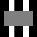
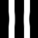
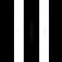
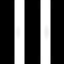
In Figure 1, we present a comparison between the proposed equation and the CHE equipped with the double-well potential for inpainting a standard binary image of stripes. The image domain is represented by a grey rectangle, which is larger than what is commonly used in the literature for this test image [5, 34]. The comparison was based on the quality of the resulting images, as well as the presence of diffusive effects introduced by the CHE. Figure 1(b) was obtained after 8000 iterations, where the first 4000 iterations were done with $\varepsilon=100$, and then $\varepsilon=1$. Furthermore, besides the irregularly reconstructed inpainting domain, we can observe the diffusive effects in the regions containing black-to-white or white-to-black transitions (edges). On the other hand, in Figure 1(c) we have recovered the sharp edges and the natural continuation of the features of the image into the inpainting domain. The image was obtained after 10000 iterations, using the same two-scale approach with $\varepsilon=100$ and then $\varepsilon=2$. As discussed later, the inpainting process seems to slow down as the inpainting domain becomes barely detectable. Even though mean-squared error (MSE) values can sometimes be in discordance with the human eye, for this example, the image obtained by the CHE resulted in an MSE of 0.0172, while the image obtained by the proposed equation has an MSE of 0.0157.

(a) Original image

(b) CH equation

(c) Proposed equation

Figure 2: Results of image inpainting for the image of a cross.

In Figure 2, we consider a cross-shaped image with a damaged region at the centre. The results of the inpainting process obtained with the CHE are presented in Figure 2(b) and are obtained after 8000 iterations, following the two-scale approach with $\varepsilon=100$, and then $\varepsilon=1$. Let us note that these results are consistent with the results obtained in previous studies (e.g., Figure 3.1 in [6], Figures 1 and 2 in [4], or Figure 3 in [9]). In the inpainted image produced by the proposed equation in Figure 2(c), we observe that it effectively restores the missing information while preserving the edges and extending the image features in a natural manner. In comparison with Figure 4 in [48], the newly formed edges in the centre of the image seem more natural and can be obtained without coupling the equation with the thresholding operation. This image was obtained after 30000 iterations with $\varepsilon=100$ and then $\varepsilon=2$.

(a) After 100 iterations

(b) After 1000 iterations

(c) After 4000 iterations

(d) After 8000 iterations

Figure 3: Snapshots of the evolution of the inpainting process for the image of a cross (as in Figure 2).

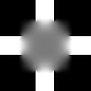
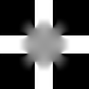
Figure 3 presents a sequence of snapshots demonstrating the progression of the inpainting process when the maximal number of iterations is set to 100, 1000, 4000, and 8000 iterations. It can be observed that the initial phase of the inpainting process is characterized by a rapid recovery of the image features. However, as the inpainting domain diminishes, the process tends to become slower, and the area of image restoration between iteration numbers 4000 and 8000 (Figure 3(c) and Figure 3(d)) is relatively modest compared to the area recovered during the initial 1000 iterations (Figure 3(a) and Figure 3(b)). The final image was obtained after 30000 iterations and is displayed in Figure 2(c).

(a) Original image

(b) Resulting image (a)

(c) Original image

(d) Resulting image (b)

Figure 4: Inpainting over the large domains.

The results of inpainting for a large inpainting domain are displayed in Figure 4, where ion can observe that the image features have been retrieved without any apparent diffusive effects. However, it is noteworthy that the process required a substantial number of iterations to restore the entire image because the size of the inpainting domain constituted approximately $60\%$ of the image size. The same parameters $\varepsilon$ were used as in Figure 1 and Figure 2, and Figure 4(b) was obtained after 20000 iterations, while Figure 4(d) was obtained after 60000 iterations.

5.2 Inpainting results for different choice of parameters

(a) Original image

(b) After 200 iterations

(c) After 1000 iterations

(d) After 4000 iterations

(e) After 8000 iterations

(f) Original image

(g) After 200 iterations

(h) After 1000 iterations

(i) After 4000 iterations

(j) After 8000 iterations

(k) Original image

(l) After 200 iterations

(m) After 1000 iterations

(n) After 4000 iterations

(o) After 8000 iterations

Figure 5: Inpainting over the large and complex domain for a different choice of parameters.

Figure 5 depicts a binary image of a cross with a hexagonal inpainting domain located in the centre of the image. Each row exhibits the temporal evolution of the inpainting process for a different choice of parameters $\varepsilon$ with a maximal number of iterations set to 200, 1000, 4000, and 8000 iterations, respectively. We can observe that the changes made inside the inpainting domain are similar for the first two experiments, that is, if the process converges, then it converges following the comparable paths. In the first experiment (Figures 5(a)-5(e)), the parameters used were $\varepsilon=5$ initially, followed by $\varepsilon=2$. The second row (Figures 5(f)-5(j)), involved the use of $\varepsilon=100$ initially, followed by $\varepsilon=2$, which was the same as in the first experiment. In the third experiment (Figures 5(k)-5(o)), we used $\varepsilon=100$ initially, and then $\varepsilon=3$, and we can notice that for this choice of parameters the inpainting domain seems to remain unchanged after the first 200 iterations.

5.3 Limitations

Upon testing the proposed equation, we observed that it exhibited suitable performance in the context of inpainting when the underlying image comprised straight lines, edges, and corners. However, for images that comprised numerous flow-like structures (for example fingerprint image), the performance was modest, and it is recommended to rely on the classical Cahn-Hilliard equation in such cases. We believe that this could be resolved by replacing the Laplacian as the edge classifier for a structure tensor as in the work of Weickert [65] to guarantee that this equation creates shocks orthogonal to the flow direction of the pattern. It is noteworthy that the selection of appropriate parameters poses a significant challenge for all PDE models, and this issue is equally relevant for this model, especially in the context of nonstandard images and large domains. For example, in Figure 5 one can notice that a small change in the $\varepsilon$ in the last experiment resulted in the incomplete inpainting of the unknown region. We have also observed that the CHE required fewer iterations to produce the inpainted images compared to the proposed method. For instance, Figure 2(b) was obtained after 8000 iterations of the two-step process, whereas Figure 2(c) was obtained after 30000 iterations. Overall, these findings suggest that the proposed equation is a viable alternative to the CHE for image inpainting, as it produces images with fewer diffusive effects, albeit requiring more iterations than the CHE. In short, these results highlight the trade-off between computational efficiency and the quality of the reconstructed images when selecting an appropriate nonlinear classifier $H$.

Conclusions and final remarks

Inspired by the inpainting methods based on the Cahn-Hilliard equation, we have introduced the fully nonlinear fourth-order PDE in which the image reconstruction is driven by the diffusion joined by the nonlinear term belonging to the class of morphological image enhancement methods. Our primary objective was to establish the well-posedness of this equation and investigate its potential for inpainting tasks.

To achieve the latter, we employed Young measures to devise a suitable solution concept. Additionally, a robust adaptation of the Kruzhkov entropy admissibility approach enabled us to address the challenging non-linearity present in the equation and to demonstrate the existence and stability of an appropriate class of solutions.

Our work not only contributes to the field of inpainting but also sheds light on the broader topic of non-linear partial differential equations in image processing. By establishing the well-posedness of our equation, we have taken a significant step towards enhancing the understanding of complex non-linear systems in this context.

The obtained results provide a solid theoretical foundation for the practical application of this inpainting model. To this end, we have utilized the idea of convexity splitting to derive a numerical scheme for practical implementation. Using the testing binary images that contain straight lines or edges in the inpainting domain, we have demonstrated that the proposed morphological classifier naturally extends image structures and preserves image sharpness, leading to superior results compared to a standard Cahn-Hilliard equation with a double-well potential. For binary shapes that contain a lot of curves (such as fingerprint image or zebra), we have noticed that the introduced equation shows more modest results and it seems to be more sensitive to changes in parameters as compared to the classical CHE.

In conclusion, we have presented a well-posed formulation of the Shock Filter Cahn-Hilliard equation for image inpainting and conducted numerical simulations in order to solidify both its theoretical foundation and demonstrate its potential for practical applications. We hope that our result will contribute toward enriching the theoretical landscape of inpainting models and providing a deeper perspective on the role of fully non-linear PDEs in image processing.

References

• [1] R. Backofen, S.M.  Wise, M. Salvalaglio, A. Voigt, Convexity splitting in a phase field model for surface diffusion, Int.J. Num. Anal. Model. 16 (2020), 192–209.
• [2] M. Bertalmio, G. Sapiro, V. Caselles and C. Ballester, Image inpainting, Proceedings of the 27th annual conference on Computer graphics and interactive techniques. ACM Press/Addison-Wesley Publishing Co., 2000.
• [3] M. Bertalmio, A. Bertozzi, and G. Sapiro, Navier-Stokes, fluid dynamics, and image and video inpainting, Computer Vision and Pattern Recognition, 2001. CVPR 2001. Proceedings of the 2001 IEEE Computer Society Conference on. Vol. 1. IEEE, 2001.
• [4] A. Bertozzi, S. Esedoglu, and A. Gillette, Inpainting of binary images using the Cahn–Hilliard equation, IEEE Transactions on Image Processing 16 (2006), 285–291.
• [5] A. Bertozzi, S. Esedoglu, A. Gillette, Analysis of a two-scale Cahn–Hilliard model for binary image inpainting, Multiscale Modeling & Simulation 6 (2007), 913–936.
• [6] A. Bertozzi, C. B. Schönlieb, Unconditionally stable schemes for higher order inpainting Comm. Math. Sci. 9 (2011), 413–457.
• [7] S. Bianchini, A. Bressan, Vanishing viscosity solutions of nonlinear hyperbolic systems, Annals of Mathematics 161 (2005), 223–342.
• [8] J. F. Blowey, C. M. Elliot, The Cahn–Hilliard gradient theory for phase separation with non-smooth free energy Part 1: Mathematical analysis, European J. Appl. Math. 2 (1991), 233–280.
• [9] J. Bosch, D.  Kay, M.  Stoll, and A.  J.  Wathen, Fast solvers for Cahn–Hilliard inpainting, SIAM J. Imaging Sci. 7 (2014), 67–97.
• [10] J. Bosch, M.  Stoll, A fractional inpainting model based on the vector-valued Cahn–Hilliard equation, SIAM J. Imaging Sci. 8 (2015), 2352–2382.
• [11] A. L. Brkić, D. Mitrovic, A. Novak, On the image inpainting problem from the viewpoint of a nonlocal Cahn-Hilliard type equation, J. Adv. Res. 25 (2020), 67–76.
• [12] A. L. Brkić, A. Novak, A nonlocal image inpainting problem using the linear Allen–Cahn equation, Conference on Non-integer Order Calculus and Its Applications. Springer, 2018.
• [13] R. Brown, Z. W. Shen, The initial-Dirichlet problem for a fourth order parabolic equation in Lipschitz cylinders, Indiana Univ. Math. J. 39 (1990), 1313–1353.
• [14] A. Buades, C. Bartomeu, M. Jean-Michel, Neighborhood filters and PDE’s, Numerische Mathematik 105 (2006), 1–34.
• [15] M. Burger, L. He, C.-B. Schönlieb, Cahn–Hilliard inpainting and a generalization for grayvalue images, SIAM J. Imaging Sci. 2 (2009), 1129–1167.
• [16] J. W.  Cahn , J. E.  Hilliard, Free energy of a nonuniform system. I. Interfacial free energy, The Journal of Chemical Physics 28 (1958), 258–267.
• [17] J. Calder, A. Mansouri, A. Yezzi, Image sharpening via Sobolev gradient flows, SIAM J. Imaging Sci. 3 (2010), 981–1014.
• [18] J. A. Carrillo, S. Kalliadasis, F. Liang, S. P. Perez, Enhancement of damagedimage prediction through Cahn–Hilliard image inpainting, R. Soc. Open Sci. 8 (2021), 201294.
• [19] M.E. Cates, E. Tjhung, Theories of binary fluid mixtures: from phase-separation kinetics to active emulsions, J. Fluid Mech. 836 (2018), P1.
• [20] T.F. Chan, J. Shen, H.-M. Zhou, Total variation wavelet inpainting, Journal of Mathematical imaging and Vision 25 (2006), 107–125.
• [21] M. Cheng, J.A.  Warren, An efficient algorithm for solving the phase field crystal model, J. of Computational Physics 227 (2008), 6241–6248.
• [22] L. Cherfils, H. Fakih, A. Miranville, A Cahn–Hilliard system with a fidelity term for color image inpainting, Journal of Mathematical Imaging and Vision 54 (2016), 117–131.
• [23] L. Cherfils, H. Fakih, A. Miranville, A complex version of the Cahn–Hilliard equation for grayscale image inpainting, Multiscale Modeling & Simulation 15 (2017), 575–605.
• [24] L. Cherfils, F. Hussein, A. Miranville, On the Bertozzi–Esedoglu–Gillette–Cahn–Hilliard equation with logarithmic nonlinear terms, SIAM J. Imaging Sci. 8 (2015), 1123–1140.
• [25] L. Cherfils, F. Hussein, A. Miranville, Finite-dimensional attractors for the Bertozzi–Esedoglu–Gillette–Cahn–Hilliard equation in image inpainting, Inverse Problems $\&$ Imaging 9 (2015), 105–125.
• [26] L. Cherfils, A. Miranville, S. Zelik, The Cahn-Hilliard equation with logarithmic potentials, Milan J. Math. 79 (2011), 561–596.
• [27] M.I.M.  Copetti, C.M. Elliott, Numerical analysis of the Cahn–Hilliard equation with a logarithmic free energy, Numerische Mathematik, 63 (1992), 39–65.
• [28] S. Dai, Q. Du, Weak Solutions for the Cahn–Hilliard Equation with Degenerate Mobility, Arch. Rational Mech. Anal. 219 (2016), 1161–1184.
• [29] R. DiPerna, A. Majda, Oscillation and concentration in weak solutions in the incompressible fluid equations, Comm. Math. Phys. 108 (1987), 667–689.
• [30] L. Escauriaza, S. Montaner, C. Zhang, Analyticity of solutions to parabolic evolutions and applications, SIAM J. Math. Anal. 49 (2017), 4064–4092.
• [31] S. Esedoglu, S.J. Osher, Decomposition of images by the anisotropic Rudin-Osher-Fatemi model, Comm. Pure App. Math. 57 (2004), 1609–1626.
• [32] S. Esedoglu, S. Jianhong, Digital inpainting based on the Mumford–Shah–Euler image model, Eur. J. App. Math. 13 (2002), 353–370.
• [33] D.J. Eyre, Unconditionally gradient stable time marching the Cahn-Hilliard equation, MRS Online Proceedings Library (OPL) 529 (1998).
• [34] H. Garcke, K. Fong Lam, and V. Styles, Cahn–Hilliard inpainting with the double obstacle potential, SIAM Journal on Imaging Sciences 11 (2018), 2064-2089.
• [35] G. Gilboa, N.  Sochen, Y.Y. Zeevi, Image enhancement and denoising by complex diffusion processes, IEEE Trans.Pattern Anal. Machine Intelligence 26 (2004), 1020–1036.
• [36] K. Glasner, S.  Orizaga, Improving the accuracy of convexity splitting methods for gradient flow equations, J. Comp. Phys. 315 (2016), 52–64.
• [37] H. Gomez, T. JR Hughes, Provably unconditionally stable, second-order time-accurate, mixed variational methods for phase-field models, J. Comp. Phys. 230 (2011), 5310–5327.
• [38] P. Fischer, J.  Mergheim, P.  Steinmann, On the C1 continuous discretization of non-linear gradient elasticity: A comparison of NEM and FEM based on Bernstein–Bézier patches, Int. J. Num. Meth. Eng. 82 (2010), 1282–1307.
• [39] D. Gilbarg, N. Trudinger, Elliptic partial differential equation of second order. Fundamental Principles of Mathematical Sciences 224. Springer-Verlag, Berlin, 1983.
• [40] D. Han, X. Wang, A second order in time, uniquely solvable, unconditionally stable numerical scheme for Cahn–Hilliard–Navier–Stokes equation, J. Comp. Phys. 290 (2015), 139–156.
• [41] H. Kalisch, D. Mitrovic, On Existence and Admissibility of Singular Solutions for Systems of Conservation Laws, Int. J. Appl. Comput. Math 8 175 (2022).
• [42] S. N. Kruzhkov, First order quasilinear equations in several independent variables, Mat.Sb. 81 (1970), 1309–1351.
• [43] C. Liu, and J. Shen, A phase field model for the mixture of two incompressible fluids and its approximation by a Fourier-spectral method, Physica D: Nonlinear Phenomena 179 (2003), 211–228.
• [44] F. Magaletti, F. Picano, M. Chinappi, L. Marino, C.  M.  Casciola, The sharp-interface limit of the Cahn–Hilliard/Navier–Stokes model for binary fluids, J. Fluid Mech. 714 (2013), 95–126.
• [45] A. Miranville, The Cahn–Hilliard equation and some of its variants, AIMS Mathematics 2 (2017), 479–544.
• [46] A. Miranville, The Cahn–Hilliard equation: recent advances and applications, Society for Industrial and Applied Mathematics, 2019.
• [47] D. Mumford, J. Shah, Optimal approximations by piecewise smooth functions and associated variational problems, Communications on Pure and Applied Mathematics 42 (1989), 577–685.
• [48] A. Novak, N. Reinić, Shock filter as the classifier for image inpainting problem using the Cahn-Hilliard equation, Comp. & Math. App. 123 (2022), 105–114.
• [49] A. Novick-Cohen, The Cahn–Hilliard equation, Handbook of differential equations: evolutionary equations 4 (2008): 201–228.
• [50] S. Osher, L.I. Rudin, Feature-oriented image enhancement using shock filters, SIAM J. Num. Anal. 27 (1990), 919–940.
• [51] S.  Parisotto, C.-B.  Schn̈lieb. MATLAB/Python Codes for the Image Inpainting Problem (3.0.1). Zenodo. (2020).
• [52] S. Pei, H. Yanren, and Y. Bo, A linearly second-order energy stable scheme for the phase field crystal model, Applied Numerical Mathematics 140 (2019), 134–164.
• [53] S. Puri, A. J. Bray, J. L. Lebowitz, Phase-separation kinetics in a model with order parameter-dependent mobility, Phys. Rev. E 56 (1997), 758.
• [54] T. Ringholm, J. Lazic, C-B. Schonlieb, Variational image regularization with Euler’s elastica using a discrete gradient scheme, SIAM J. Imaging Sci. 11 (2018), 2665–2691.
• [55] T. Roubícek, Nonlinear partial differential equations with applications, Vol. 153. Springer Science, 2013.
• [56] L.I. Rudin, S.  Osher, E.  Fatemi, Nonlinear total variation based noise removal algorithms, Physica D: Nonlinear Phenomena 60 (1992), 259–268.
• [57] J. Shen, S. H. Kang, and T. F.  Chan, Euler’s elastica and curvature–based inpainting, SIAM Journal on Applied Mathematics 63 (2003), 564–592.
• [58] J. Shen, T. F. Chan, Mathematical models for local nontexture inpaintings, SIAM J. App. Math. 62 (2002), 1019–1043.
• [59] J. Shin, and H. G.  Lee, A linear, high-order, and unconditionally energy stable scheme for the epitaxial thin film growth model without slope selection, Applied Numerical Mathematics 163 (2021): 30-42.
• [60] J. Shin, H. Geun, J. Lee, Unconditionally stable methods for gradient flow using convex splitting Runge-Kutta scheme, J. Comput. Phys. 347 (2017), 367–381.
• [61] V. R.Simi, D. Reddy Edla, J. Joseph, An inverse mathematical technique for improving the sharpness of magnetic resonance images, J. Ambient Intelligence and Humanized Computing 14 (2023), 2061–2075.
• [62] X.-C. Tai, J.  Hahn, G. J. Chung, A fast algorithm for Euler’s elastica model using augmented Lagrangian method, SIAM J. Imaging Sci. 4 (2011), 313–344.
• [63] D.N.H.  Thanh, VB Surya Prasath, S. Dvoenko, An adaptive image inpainting method based on Euler’s elastica with adaptive parameters estimation and the discrete gradient method, Signal Processing 178 (2021), 107797.
• [64] A. Tsai, A.  Yezzi, A. S.  Willsky, Curve evolution implementation of the Mumford-Shah functional for image segmentation, denoising, interpolation, and magnification, IEEE Trans. Image Process. 10 (2001), 1169–1186.
• [65] J.  Weickert, Coherence-enhancing shock filters. Pattern Recognition: 25th DAGM Symposium, Magdeburg, Germany, September 10-12, 2003. Proceedings 25. Springer Berlin Heidelberg, 2003.
• [66] X. Yang, Numerical approximations for the Cahn–Hilliard phase field model of the binary fluid-surfactant system, J. Sci. Computing 74 (2018), 1533–1553.
• [67] M.A. Zaks, A.  Podolny, A. A.  Nepomnyashchy and A. A.  Golovin, Periodic stationary patterns governed by a convective Cahn–Hilliard equation, SIAM J. App. Math. 66 (2005), 700–720.
• [68] W. Zhu, X.-C. Tai, T. Chan, Augmented Lagrangian method for a mean curvature based image denoising model, Inverse Probl. Imaging 7 (2013), 1409–1432.
• [69] H. Zhao, B.D.  Storey, R.D.  Braatz, M.Z.  Bazant Learning the physics of pattern formation from images, Phys. Rev. Lett. 124 (2020), 060201.