CAFE: Conflict-Aware Feature-wise Explanations

Abstract

Feature attribution methods are widely used to explain neural models by determining the influence of individual input features on the models’ outputs. We propose a novel feature attribution method, CAFE (Conflict-Aware Feature-wise Explanations), that addresses three limitations of the existing methods: their disregard for the impact of conflicting features, their lack of consideration for the influence of bias terms, and an overly high sensitivity to local variations in the underpinning activation functions. Unlike other methods, CAFE provides safeguards against overestimating the effects of neuron inputs and separately traces positive and negative influences of input features and biases, resulting in enhanced robustness and increased ability to surface feature conflicts. We show experimentally that CAFE is better able to identify conflicting features on synthetic tabular data and exhibits the best overall fidelity on several real-world tabular datasets, while being highly computationally efficient.

1 INTRODUCTION

Feature attribution methods, which aim to determine the effects of individual features on the predictions of machine learning models, are popular approaches for post-hoc explainability (Guidotti et al.,, 2018; Zhang et al.,, 2021). Such methods include, amongst others, LIME (Ribeiro et al.,, 2016), SHAP (Lundberg and Lee,, 2017), Gradient $\cdot$ Input (Shrikumar et al.,, 2016), LRP (Bach et al.,, 2015), DeepLIFT (Shrikumar et al.,, 2017), Integrated Gradients (Sundararajan et al.,, 2017) and SmoothGrad (Smilkov et al.,, 2017). Feature attribution scores can surface useful insights about models, including bugs and biases (Pezeshkpour et al.,, 2021; Meng et al.,, 2022).

It is generally agreed that fidelity of explanations to models is important (Yeh et al.,, 2019; Sokol and Flach,, 2020; Nauta et al.,, 2023) and, when a model is faced with unclear or partially contradictory inputs, a faithful explanation method should be capable of unearthing such conflicts (Wang and Nvasconcelos,, 2019). For example, consider a healthcare AI system predicting a patient’s risk of death based on vital signs and previous treatments. When faced with a normal temperature reading, the system may typically predict a lower overall risk, but this line of reasoning may be suppressed when the patient was recently administered an antipyretic drug. A faithful explanation should surface this internal conflict instead of simply concluding that the body temperature reading and antipyretic drug administration had no effect on the prediction.

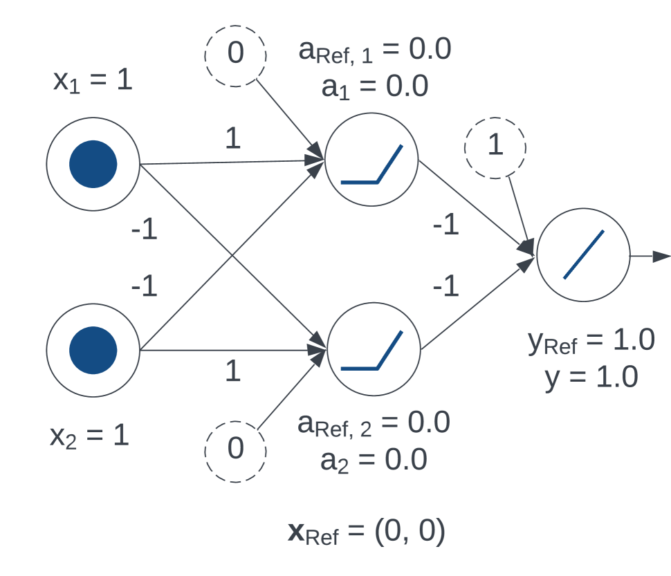
(a) XNOR NN

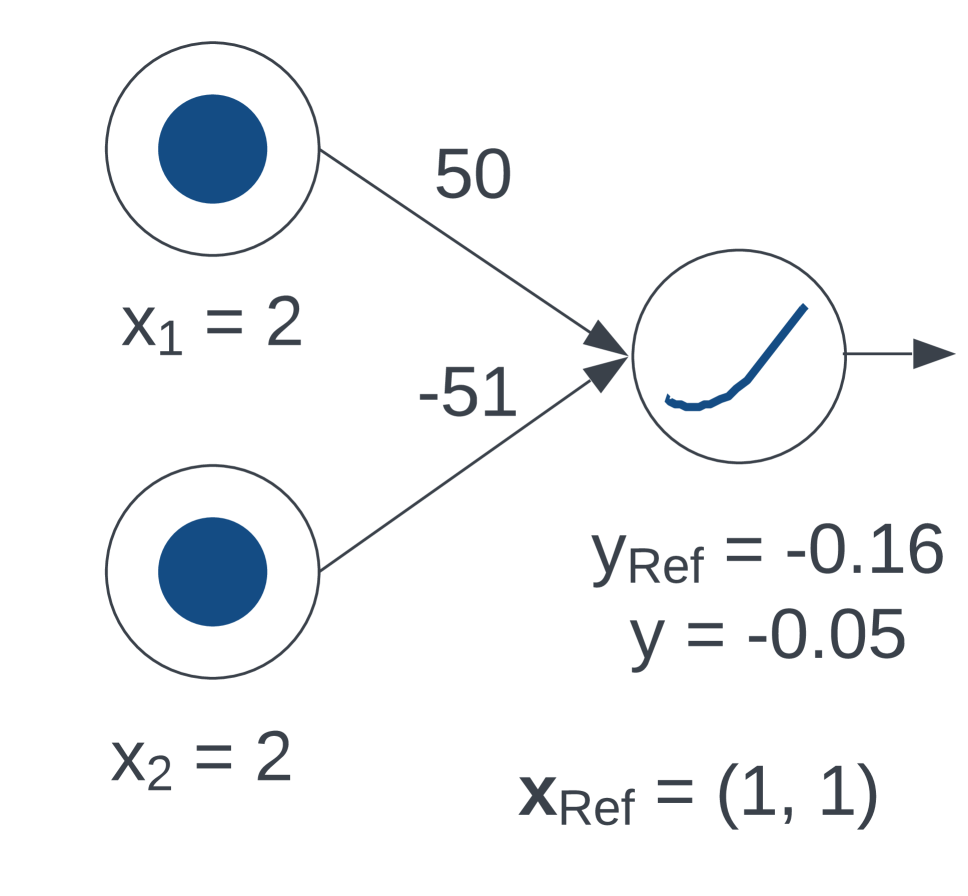
(b) GELU NN

Method	Attribution Scores
	$x_{1}$	$x_{2}$
G $\cdot$ I	-8.52	8.69
LRP	2.28	-2.32
DL-R	-5.66	5.77
DL-RC	24.56	-24.44
IG	-5.66	5.77
CAFE (0.0)	+0.0/-0.05	+0.16/-0.0
CAFE (1.0)	+49.16/-0.05	+0.16/-49.16

(c) Attribution scores returned by the different attribution methods for the GELU NN in Figure 1(b)

Figure 1: Illustrations of the issues addressed by CAFE (where 0.0 and 1.0 in brackets reflect conflict sensitivity, see Section 4), with Gradient $\cdot$ Input (G $\cdot$ I), LRP, DeepLIFT Rescale (DL-R), DeepLIFT RevealCancel (DL-RC) and Integrated Gradients (IG) as baselines. For the XNOR NN (Figure 1(a)), all baselines disregard conflicting features and biases, returning zero feature attributions. Meanwhile, CAFE (1.0) returns +1/-1 for both features and 1 for the bias. For the GELU NN (Figure 1(b)), Figure 1(c) shows that G $\cdot$ I, DL-R and IG return erroneous scores for both features, significantly overestimating their possible effect on the output; LRP and DL-RC do not exhibit the attribution explosion issue here, but their scores still do not fully capture conflicting features.

Existing feature attribution methods often fail to unearth conflicts. For example, consider the neural network model (NN) in Figure 1(a), computing the binary XNOR function (which is $0$ if exactly one of the two binary inputs is $1$ and $1$ otherwise), and the input ${\bm{x}}=(1,1)$. By inspection of the weights and neuron activations, it is clear that the input features are in conflict, pushing the pre-activations of both hidden neurons to zero values for which the ReLU function is inactive. This causes all gradient-based feature attribution methods to return zero attribution scores for both input features, thus failing to surface that the features were considered but eventually cancelled out. Additionally, since the input features cancel each other symmetrically and since the NN output is driven by the $+1$ bias of the output neuron, even methods that are not gradient-based and are explicitly designed to handle conflicts (notably DeepLIFT RevealCancel) return zeros. This simple example also illustrates another common deficiency of existing feature attribution methods — that they ignore the effect of the bias terms on predictions and may thus provide an incomplete understanding of the NN behaviour.

Another desirable property for feature attribution methods is robustness to local variations in the model activations and, by extension, its gradients, especially since NNs and their gradients can be highly irregular (Balduzzi et al.,, 2017). Instead, many existing feature attribution methods are prone to what we call “attribution score explosion”, which can cause the attribution scores to become unreasonably low or high, far beyond the model’s actual output range. For illustration, consider the NN in Figure 1(b), input ${\bm{x}}=(2,2)$ and reference input ${\bm{x}}_{\text{ref}}=(1,1)$. Figure 1(c) shows that all methods except for LRP and DeepLIFT RevealCancel assign large negative scores to $x_{1}$ and large positive scores to $x_{2}$. While these scores somewhat capture the local behaviour of the GELU activation function, they significantly overstate the effects of each feature. Indeed, since GELU flattens and tends to $0$ as its input becomes increasingly negative, the highest amount by which $x_{2}$ as a negative feature can increase the output from the reference value $y_{\text{ref}}=-0.16$ is $0.16$. The positive attribution scores returned for $x_{2}$ are thus unreasonably high. Meanwhile, although the scores from LRP and DeepLIFT RevealCancel show that $x_{1}$ could also have a positive effect, they only illustrate fractions of this hypothetical effect and also mask the actual small negative effect of $x_{1}$ in the negative range of GELU. Instead, it may be useful to capture both positive and negative effects of features, and to be able to control the degree to which the hypothetical, cancelled features’ effects are reflected in the attribution scores.

We introduce a new feature attribution method for NNs, CAFE (Conflict-Aware Feature-wise Explanations), designed to overcome these issues while also (i) allowing users to control how much (if any) of the cancelled effects should be captured in the produced attribution scores (via a conflict sensitivity hyper-parameter) and (ii) being computable in a single pass through the explained NNs. Our experimental results show that CAFE produces the most accurate attribution scores on synthetic tabular data with conflicting features and achieves the overall best fidelity when applied to four datasets and models from the OpenXAI benchmark (Agarwal et al.,, 2022) as well as a mortality prediction model trained on (a subset of) the MIMIC-IV medical database (Johnson et al.,, 2023).

2 RELATED WORK

Most relevant to our work are feature attribution methods, which quantify the importance of each input feature with respect to the output of a machine learning model. Amongst these, simple gradients (Simonyan et al.,, 2013) or gradients multiplied with the inputs (Shrikumar et al.,, 2016) capture NNs’ behavior in a small vicinity around the input, which may not represent the overall behavior when the models represent irregular or saturated functions. As an alternative to using raw gradients, several enhanced gradient-based attribution methods have been proposed, including LRP (Bach et al.,, 2015; Montavon et al.,, 2019), DeepLIFT Rescale (Shrikumar et al.,, 2017) and Integrated Gradients (Sundararajan et al.,, 2017). These methods may not reflect the effects of conflicting features and also exhibit other limitations, as illustrated in Section 1. CAFE borrows from DeepLIFT and Integrated Gradients the use of a specified reference input to compute explanations.

Some feature attribution methods are model-agnostic. For instance, LIME (Ribeiro et al.,, 2016) produces feature attribution scores by approximating any model using an interpretable linear model. Meanwhile, Shapley Value Sampling (Strumbelj and Kononenko,, 2010) and SHAP (Lundberg and Lee,, 2017) leverage Shapley values (Shapley,, 1953) from game theory to assess feature importance. These methods, however, often necessitate extensive sampling and multiple model evaluations, making them computationally demanding.

Two attribution methods are particularly relevant to our goals of accounting for conflicts and biases. DeepLIFT RevealCancel (Shrikumar et al.,, 2017) uses an approximation of Shapley values for surfacing cancelled features, to some extent, but suffers from other limitations, as illustrated in Section 1. Bias Back-propagation (Wang et al.,, 2019) attributes the effects of biases to input features, differing from CAFE, which computes separate attribution scores for input features and biases, thus distinguishing between the two.

CAFE aims to better understand the reasoning of NNs, by unearthing conflicts between features and the role of biases. Similarly, existing work on deliberative explanations  (Wang and Nvasconcelos,, 2019) emphasized the importance of capturing insecurities in NNs, though it focused exclusively on images and produced sets of potentially ambiguous input regions instead of attribution scores, making it orthogonal to our approach. Also related to internal model deliberations are contrastive explanations with pertinent negatives (Dhurandhar et al.,, 2018), which highlight the missing parts of inputs that could cause the model to predict different classes, making them closer in spirit to counterfactual explanations. Finally, SpArX (Ayoobi et al.,, 2023) aims at tracking the full reasoning of NNs through their sparsification. However, the produced explanations are considerably more complex than attribution scores and may not scale to larger NNs.

Evaluating AI model explanations, including feature attributions, remains an open research area, with a general lack of standardisation and a variety of discordant viewpoints on what constitutes a more desirable explanation (Zhou et al.,, 2021; Chen et al.,, 2022; Rahnama,, 2023; Nauta et al.,, 2023; Le et al.,, 2023). Several properties have been proposed and studied in the literature (e.g. see (Sokol and Flach,, 2020; Nauta et al.,, 2023) for some overviews). Amongst these, fidelity (also referred to as correctness, faithfulness or descriptive accuracy (Nauta et al.,, 2023)) is widely regarded as crucial (Yeh et al.,, 2019), as it amounts to explanations being truthful to the model they aim to explain: we will use this measure for comparison between CAFE and several baselines. CAFE is also designed to satisfy the commonly enforced completeness property (Sundararajan et al.,, 2017) (also known as “summation-to-delta” (Shrikumar et al.,, 2017) or “sensitivity-N” (Ancona et al.,, 2018)), requiring that the sum of the attribution scores should be equal to the difference between the model outputs for the reference input and for the actual input. Finally, we consider properties of missingness from (Lundberg and Lee,, 2017) and linearity from Sundararajan et al., (2017).

3 PRELIMINARIES

Our goal is to explain an NN $\mathcal{M}:\mathbb{R}^{\text{dim}(0)}\rightarrow\mathbb{R}^{\text{dim}(N)}$ with $N$ layers, taking inputs of dimension $\text{dim}(0)$ and returning outputs of dimension $\text{dim}(N)$. We view $\mathcal{M}$ as composed of layers $L^{(1)},\ldots,L^{(N)}$, where $L^{(1)}$ is the input layer and $L^{(N)}$ is the output layer. When referring to the vector of activation values of the neurons in layer $L^{(n)}$ ($1\!\leq\!n\!\leq\!N$), we use the notation ${\bm{a}}^{(n)}$.

In order to simplify our definitions, we assume that linear transformations and applications of activation functions are performed by distinct layers. A linear layer $L^{(n+1)}$ computes the operation ${\bm{a}}^{(n+1)}={\bm{W}}^{(n+1)\top}{\bm{a}}^{(n)}+{\bm{b}}^{(n+1)}$ where ${\bm{a}}^{(n)}\in\mathbb{R}^{\text{dim}(n)}$ is the output of the previous layer, ${\bm{a}}^{(n+1)}\in\mathbb{R}^{\text{dim}(n+1)}$ is the layer output, ${\bm{W}}^{(n+1)}\in\mathbb{R}^{\text{dim}(n)\times\text{dim}(n+1)}$ is the weight matrix and ${\bm{b}}^{(n+1)}\in\mathbb{R}^{\text{dim}(n+1)}$ is the bias vector. As conventional, we refer to the individual elements of ${\bm{W}}^{(n+1)}$ and ${\bm{b}}^{(n+1)}$ as ${W}^{(n+1)}_{i,j}$ and ${b}^{(n+1)}_{j}$, respectively, where $i$ and $j$ are indexes to neurons in layer $L^{(n)}$ and $L^{(n+1)}$, respectively. An activation layer $L^{(n+1)}$ computes the operation $\textbf{a}^{(n+1)}=\phi^{(n+1)}(\textbf{a}^{(n)})$ for some activation function $\phi^{(n+1)}$. The input and output dimensions, $\text{dim}(n)$ and $\text{dim}(n+1)$ respectively, of an activation layer are always identical. When dealing with classification models, we disregard the final softmax layer, as this has been argued to result in more intuitive model explanations (Shrikumar et al.,, 2017).

Our problem of interest is computing the positive attribution scores ${\bm{S}}^{+}\in\mathbb{R}^{(\text{dim}(0)+1)\times\text{dim}(N)}$ and the negative attribution scores ${\bm{S}}^{-}\in\mathbb{R}^{(\text{dim}(0)+1)\times\text{dim}(N)}$ (with $\text{dim}(0)$ feature attribution scores and one extra bias attribution score for each output neuron) for $\mathcal{M}({\bm{x}})$, given some input ${\bm{x}}\in\mathbb{R}^{\text{dim}(0)}$ and a reference input ${\bm{x}}_{\text{ref}}\in\mathbb{R}^{\text{dim}(0)}$. The latter can be any suitable baseline in the given context, e.g. mean or median feature values, zeroes or random noise. We will use the notation $x_{f}$ and $x_{\text{ref},f}$ to refer to the individual features of the actual input and the reference input, respectively, with $f\in\{1,2,\dots,\text{dim}(0)\}$ acting as the feature index. We will also consider the joint scores ${\bm{S}}^{*}\!=\!{\bm{S}}^{+}\!-\!{\bm{S}}^{-}$. When computing the attribution scores, we will consider a version of $\mathcal{M}$, denoted $\mathcal{M}_{\text{ref}}$, with all biases ablated (i.e. set to $0$). We will refer to $\mathcal{M}_{\text{ref}}$’s activation values at layer $L^{(n)}$ when applied to ${\bm{x}}_{\text{ref}}$ as ${\bm{a}}^{(n)}_{\text{ref}}$.

Finally, to refer to the intermediate (positive or negative) feature attribution scores computed at layer $L^{(n)}$ for feature $f$ and neuron $i$, we will use the notation $S^{(n),+}_{f,i}$ and $S^{(n),-}_{f,i}$, respectively. Similarly, we will refer to the intermediate bias attribution scores as $S^{(n),+}_{\text{bias},i}$ and $S^{(n),-}_{\text{bias},i}$. We will also use sign variables $\sigma$ and $\tau$ to refer to a value from $\{+,-\}$. In a slight abuse of notation, we will sometimes employ $\sigma$ and $\tau$ as operators that are ignored if referring to the $+$ sign and that flip the sign of the operand if referring to the $-$ sign, e.g. $\sigma(5)=-5$ if $\sigma=-$ and $\tau(-5)=-5$ if $\tau=+$.

4 EXPLAINING NNs WITH CAFE

CAFE aims to quantify how much each input feature contributes to the NN’s output and (optionally) the effects these features could have on the output if they were not in conflict with each other. Thus, unlike other methods, CAFE returns two separate scores for each feature — separately capturing its overall positive and negative effects. This is crucial for uncovering conflicts between features, including cases in which a single feature is “controversial”, i.e., it affects the output both positively and negatively. In addition to scores for the inputs, CAFE also returns aggregated scores for the bias terms, indicating how much these biases affected the output compared to the input features. This may highlight cases where predictions are primarily driven by the NN biases rather than the input. We introduce the CAFE rules for the individual NN components below, while providing examples in the supplement.

4.1 Input Layer Rule

This rule simply requires that the scores amount to the absolute difference between each actual input feature and reference input feature, as captured below.

Definition 1 (Attribution Scores (Input Layer Rule)).

The input layer attribution scores for input ${\bm{x}}$ and reference input ${\bm{x}}_{\text{ref}}$ are defined as follows (for $f\in\{1,2,\dots,\text{dim}(0)\}$ the feature index, $i\in\{1,2,\dots,\text{dim}(1)\}$ the index of a neuron in the input layer $L^{(1)}$ and $\sigma\in\{+,-\}$ as in Section 3):

$$S^{(1),\sigma}_{f,i} =\begin{cases}\max(\sigma(x_{f}-x_{\text{ref},f}),0)&\text{if $f=i$}\\ 0&\text{otherwise}\end{cases}$$

$$S^{(1),\sigma}_{\text{bias},i} =0$$

Note that, as there is not yet any interaction between features, all scores are set to $0$ except for the feature attribution scores of input neurons, which are set to the corresponding (positive or negative) differences between the reference inputs and the actual inputs.

4.2 Linear Layer Rule

The propagation of scores through a linear layer is similar to performing a standard forward pass — we simply multiply the attribution scores by the edge weights and sum them together, adding the bias term in the end. However, to distinguish between the positive and negative effects, we consider the positive and negative edge weights and biases separately, as follows.

Definition 2 (Attribution Scores (Linear Layer Rule)).

The attribution scores for the $j$-th neuron in a linear layer $L^{(n+1)}$ are:

$$S^{(n+1),\sigma}_{f,j} =\sum_{i}^{|L^{(n)}|}\Bigl{(}\max(\sigma({W}^{(n+1)}_{i,j}),0)S^{(n),+}_{f,i}$$

$$\phantom{=\sum_{i}^{|L^{(n)}|}\Bigl{(}}+\max(\sigma(-{W}^{(n+1)}_{i,j}),0)S^{(n),-}_{f,i}\Bigr{)}$$

$$S^{(n+1),\sigma}_{\text{bias},j} =\sum_{i}^{|L^{(n)}|}\Bigl{(}\max(\sigma({W}^{(n+1)}_{i,j}),0)S^{(n),+}_{\text{bias},i}$$

$$\phantom{=\sum_{i}^{|L^{(n)}|}\Bigl{(}}+\max(\sigma(-{W}^{(n+1)}_{i,j}),0)S^{(n),-}_{\text{bias},i}\Bigr{)}$$

$$\phantom{=d}+\max(\sigma({b}^{(n+1)}_{j}),0)$$

4.3 Activation Rule

Defining the rule for propagating scores through non-linear activations is a considerably greater challenge, as the effects of the non-linearities cannot be precisely captured by linear scores, forcing us to approximate. A possible approach is to compute attribution scores as for the linear layers, by considering a linear approximation of the activation function, with a slope identical to the mean slope on the interval between the reference activation (for ${\bm{x}}_{\text{ref}}$) and the actual activation (for ${\bm{x}}$). This approach, similar in spirit to DeepLIFT Rescale and Integrated Gradients, is insufficient for achieving our goals, as illustrated in Section 1.

We choose instead to additionally consider the behaviour of the activation function on the wider range spanned by the competing positive and negative effects at the given neuron, so as to estimate the hypothetical effect each feature could have if it was not cancelled as a result of the interaction with the other features. Additionally, this approach allows us to ensure that attribution scores do not become excessively high or low for extreme inputs (see Definition 2 and the associated text for details). In order to use this strategy, we first define several intermediate notions, eventually leading to Definition 8. We first define the notion of positive, negative and combined input effects on a given neuron:

Definition 3 (Input Effects (Activation Rule)).

The input effects at the $j$-th neuron in activation layer $L^{(n+1)}$ are defined as follows:

$${e}^{(n+1),\sigma}_{j} =\sigma\left(S^{(n),\sigma}_{\text{bias},j}+\sum_{f}^{|{\bm{x}}|}S^{(n),\sigma}_{f,j}\right)$$

$${e}^{(n+1),*}_{j} ={e}^{(n+1),+}_{j}+{e}^{(n+1),-}_{j}$$

with ${e}^{(n+1),\sigma}_{j}$ the positive/negative input effect for $\sigma=+$/$-$, respectively, and ${e}^{(n+1),*}_{j}$ the combined effect.

Intuitively, the positive and negative effects capture the total positive and negative deviations from the reference pre-activation (i.e. pre-activation for ${\bm{x}}_{\text{ref}}$ when all biases are ablated) at the given neuron. We can then specify how much the activation function values change on intervals of interest, as follows:

Definition 4 (Rectified Activation Deltas (Activation Rule)).

Let $L^{(n+1)}$ be an activation layer applying an activation function $\phi^{(n+1)}$, and let:

$${a}^{(n+1),\sigma}_{j} =\phi^{(n+1)}({a}^{(n)}_{\text{ref},j}+{e}^{(n+1),\sigma}_{j})$$

$${a}^{(n+1),*}_{j} =\phi^{(n+1)}({a}^{(n)}_{\text{ref},j}+{e}^{(n+1),*}_{j})$$

$${a}^{(n+1),\text{ref}}_{j} ={a}^{(n+1)}_{\text{ref},j}=\phi^{(n+1)}({a}^{(n)}_{\text{ref},j})$$

Further, let the auxiliary rectified activation deltas be:

$$\Delta^{(n+1),(\circ\rightarrow\bullet),d}_{j}\!=\!\begin{cases}\max({a}^{(n+1),\bullet}_{j}\!-\!{a}^{(n+1),\circ}_{j},0)&\text{if $d\!=\!\nearrow$}\\ \max({a}^{(n+1),\circ}_{j}\!-\!{a}^{(n+1),\bullet}_{j},0)&\text{if $d\!=\!\searrow$}\end{cases}$$

where $\circ,\bullet\in\{+,-,*,\text{ref}\}$ specify the activation delta boundary points while $d\in\{\nearrow,\searrow\}$ denotes the positive/negative slope along which the activation delta is computed. Then, the rectified activation deltas are:

$$\Delta^{(n+1),*,d}_{j}=\begin{cases}\Delta^{(n+1),(\text{ref}\rightarrow*),d}_{j}&\text{if ${e}^{(n+1),*}_{j}\geq 0$}\\ \Delta^{(n+1),(*\rightarrow\text{ref}),d}_{j}&\text{otherwise}\end{cases}$$

$$\Delta^{(n+1),+,d}_{j}=\begin{cases}\Delta^{(n+1),(*\rightarrow+),d}_{j}&\text{if ${e}^{(n+1),*}_{j}\geq 0$}\\ \Delta^{(n+1),(\text{ref}\rightarrow+),d}_{j}&\text{otherwise}\end{cases}$$

$$\Delta^{(n+1),-,d}_{j}=\begin{cases}\Delta^{(n+1),(-\rightarrow\text{ref}),d}_{j}&\text{if ${e}^{(n+1),*}_{j}\geq 0$}\\ \Delta^{(n+1),(-\rightarrow*),d}_{j}&\text{otherwise}\end{cases}$$

where $d\in\{\nearrow,\searrow\}$ is a positive/negative slope. Here, $\Delta^{(n+1),*,d}_{j}$ is the rectified activation delta for the combined effect, $\Delta^{(n+1),+,d}_{j}$ is the rectified activation delta for the positive effect and $\Delta^{(n+1),-,d}_{j}$ is the rectified activation delta for the negative effect.

On a high level, the $\Delta^{(n+1),*,d}_{j}$ rectified activation delta indicates the actual changes in the activation value at a particular neuron in comparison to its reference activation. Meanwhile, the $\Delta^{(n+1),+,d}_{j}$ and $\Delta^{(n+1),-,d}_{j}$ activation deltas capture the hypothetical changes in the activation values if the positive and negative influences at the given neuron did not partially cancel. This is instrumental to our goals of handling conflicting features and limiting the feature attribution scores to realistic values. We provide a more thorough explanation of rectified activation deltas in the supplement.

We now define the peak impact of positive/negative inputs on positive/negative outputs of activation layer neurons:

Definition 5 (Peak Attribution Flows (Activation Rule)).

The peak attribution flows at the $j$-th neuron in activation layer $L^{(n)}$ are defined as follows:

$$p^{(n),(\sigma\rightarrow\tau)}_{j}=\begin{cases}\mathds{1}[\sigma({e}^{(n),*}_{j})\geq 0]\Delta^{(n),*,\nearrow}_{j}\\ \phantom{}+\max(\Delta^{(n),+,\nearrow}_{j},\Delta^{(n),-,\nearrow}_{j})&\text{if $\sigma=\tau$}\\ \mathds{1}[\sigma({e}^{(n),*}_{j})\geq 0]\Delta^{(n),*,\searrow}_{j}\\ \phantom{}+\max(\Delta^{(n),+,\searrow}_{j},\Delta^{(n),-,\searrow}_{j})&\text{otherwise}\\ \end{cases}$$

We refer to $p^{(n),(\sigma\rightarrow\tau)}_{j}$ as the peak attribution flow from $\sigma$-signed inputs to $\tau$-signed outputs.

Intuitively, peak attribution flows establish the maximum impact of inputs on outputs of activation layer neurons, including both the “real” effects (i.e., the actual observed change in the neurons’ output with respect to the reference) and the hypothetical, cancelled effects from the conflicting features. To this end, the peak flows are computed by summing the corresponding rectified activation delta for the combined effect (capturing the “real” component) and the maximum rectified activation delta for the positive and negative effects (capturing the hypothetical, cancelled component). Note that the hypothetical effects from positive and negative inputs will never arise simultaneously, which is why they are combined using a maximum. Separating the rectified activation deltas for positive and negative slopes then enables us to accurately attribute the changes in activation function values to their respective combinations of positive/negative inputs and outputs. Note also that this definition maintains the completeness property, as the real output effect can be recovered by subtracting the peak flows for negative targets from those for positive targets.

The next notion is analogue to peak attribution flows but incorporates the real, currently observable effects from the inputs, potentially ignoring the hypothetical effects of conflicting features, as follows.

Definition 6 (Clipped Linear Attribution Flows (Activation Rule)).

The clipped linear attribution flows at $j$-th neuron in activation layer $L^{(n)}$ are:

$$l^{(n),(\sigma\rightarrow\tau)}_{j}=\begin{cases}\min\biggl{(}|{e}^{(n),\sigma}_{j}|\frac{\Delta^{(n),*,\nearrow}_{j}}{|{e}^{(n),*}_{j}|+\epsilon},\\ \phantom{\min\biggl{(}}p^{(n),(\sigma\rightarrow\tau)}_{j}\biggr{)}&\text{if $\sigma=\tau$}\\ \min\biggl{(}|{e}^{(n),\sigma}_{j}|\frac{\Delta^{(n),*,\searrow}_{j}}{|{e}^{(n),*}_{j}|+\epsilon},\\ \phantom{\min\biggl{(}}p^{(n),(\sigma\rightarrow\tau)}_{j}\biggr{)}&\text{otherwise}\\ \end{cases}$$

where $\epsilon$ is a small positive stabiliser enforcing the behaviour $\frac{0}{0}\!=\!0$. We refer to $l^{(n),(\sigma\rightarrow\tau)}_{j}$ as linear attribution flow from $\sigma$-signed inputs to $\tau$-signed outputs.

Thus, the clipped linear attribution flows are computed as a minimum of two quantities: the first estimates the attribution score flows by a linear approximation of the activation function on the interval between the reference activation and the current activation for the given input ${\bm{x}}$; the second is the peak attribution flows from Definition 5. The former ensures that the score flows are grounded in the actual behaviour of the activation function on its active interval, spanned by the reference pre-activation and the pre-activation for the current input. The latter avoids possible attribution score explosions by clipping the attribution score flows obtained by the (imprecise) linear approximation if they exceed the maximum achievable activation function values for extreme inputs.

The last auxiliary notion we need before defining attribution scores are attribution multipliers:

Definition 7 (Attribution Multipliers (Activation Rule)).

The attribution multipliers for the $j$-th neuron in activation layer $L^{(n)}$ are:

$$m^{(n),(\sigma\rightarrow\tau)}_{j} =\frac{(1-c^{(n)})l^{(n),(\sigma\rightarrow\tau)}_{j}+c^{(n)}p^{(n),(\sigma\rightarrow\tau)}_{j}}{|{e}^{(n),\sigma}_{j}|+\epsilon}$$

where $\epsilon$ is a small positive stabiliser enforcing $\frac{0}{0}\!=\!0$ and $c^{(n)}$ is the conflict sensitivity constant, $0\leq c^{(n)}\leq 1$, specifying how much to capture the cancelled effects of conflicting features. We refer to $m^{(n),(\sigma\rightarrow\tau)}_{j}$ as the multiplier from $\sigma$-signed to $\tau$-signed scores.

The attribution multipliers compute a weighted average of the corresponding capped linear attribution flows and the peaked attribution flows. The weights of the two components are customisable by the user-provided constant $c^{(n)}$, which can differ for every activation layer. This enables the end-users to decide how much to reflect the hypothetical effects of conflicting features in the resulting feature attribution scores. Values of $c^{(n)}$ closer to $0$ typically result in more focused attribution scores while the values closer to $1$ encourage greater sensitivity to conflicts between the individual features. The multipliers are also normalised by the corresponding positive/negative input effects. This ensures that the total attribution flows reflected in the peak and linear flows are redistributed between the individual features proportionally to their contribution to the total positive/negative input effects.

Finally, the attribution scores for activation layers are:

Definition 8 (Attribution Scores (Activation Rule)).

The attribution scores for $j$-th neuron and $f$-th feature from input ${\bm{x}}$ at activation layer $L^{(n+1)}$ are:

$$S^{(n+1),\sigma}_{\text{idx},j} =m^{(n+1),(+\rightarrow\sigma)}_{j}S^{(n),+}_{\text{idx},j}+m^{(n+1),(-\rightarrow\sigma)}_{j}S^{(n),-}_{\text{idx},j}$$

where $\text{idx}\in\{1,\ldots,\text{dim}(0),\text{bias}\}$.

5 EVALUATION

Here, we focus on the following aspects: theoretical properties providing guarantees on CAFE’s behaviour for any NN, computational complexity, ability to produce correct attribution scores on synthetic data with conflicting features and fidelity of CAFE’s attribution scores for models trained on real-world datasets.

5.1 Theoretical Analysis

We prove that CAFE satisfies (adapted variants) three desirable properties from the literature. Missingness, considered by Lundberg and Lee, (2017) for SHAP, requires that missing features are always assigned a zero attribution score. Linearity, one of the axioms for Integrated Gradients (Sundararajan et al.,, 2017), requires that the attribution scores preserve any linear behaviour, that is, for a model formed as a linear combination of two other models, the attribution scores should be the result of applying the same linear combination to the scores for the two constituent models. Finally, completeness requires that the attribution scores exactly account for all the changes to the model output caused by the input features.

Theorem 1.

CAFE satisfies missingness, linearity and completeness for any choice of conflict sensitivity constants $c^{(n)}$ for the individual layers.

The proof as well as the precise definitions of the properties are provided in the supplement. Note that we adapted the original definitions so that they are applicable to CAFE with its unique properties.

In the supplement, we also show that the time complexity of CAFE is $\mathcal{O}(C\cdot\text{dim}(0))$, where $C$ is the cost of the forward function associated with the explained NN. We show that, with batching, the runtimes of CAFE are comparable to gradient-based methods and significantly better than methods requiring sampling.

Table 1: Performance of different attribution methods in our synthetic data experiments for different continuous data dimensions $D$, conflict likelihoods $l$, hidden layer dimensions $H$ and activation functions $\phi$. We report the RMSE errors on the validation (VE) and test (TE) sets. Results in each row are averaged over five differently initialised datasets and NNs (the standard deviations and statistical measures are reported in the supplement). The methods are Gradient $\cdot$ Input (G $\cdot$ I), LRP, DeepLIFT Rescale (DL-R), Integrated Gradients (IG), SmoothGrad (SG), Gradient SHAP (GS), Kernel SHAP (KS), Shapley Value Sampling (SVS), LIME, and CAFE (with different values of $c^{(n)}$ for all $n$).

$D$	$l$	$H$	$\phi$	VE	TE	Attribution RMSE ($\downarrow$)
						G $\cdot$ I	LRP	DL-R	IG	SG	GS	KS	SVS	LIME
2	0.30	16	ReLU	0.03	0.07	3.27	3.27	3.19	3.18	4.86	3.19	1.81	1.59	1.69
3	0.25	24		0.02	0.04	2.66	2.66	2.57	2.59	3.96	2.59	1.60	1.27	1.49
4	0.20	32		0.10	0.08	2.57	2.57	2.46	2.47	4.33	2.49	1.66	1.29	1.51
5	0.15	40		0.09	0.11	2.13	2.13	2.04	2.06	4.25	2.07	1.53	1.12	1.33
2	0.30	16	GELU	0.02	0.06	3.28	3.14	3.07	3.07	4.89	3.09	1.81	1.59	1.69
3	0.25	24		0.03	0.04	2.68	2.56	2.50	2.52	3.94	2.53	1.60	1.27	1.48
4	0.20	32		0.09	0.09	2.55	2.37	2.24	2.28	4.27	2.30	1.66	1.29	1.51
5	0.15	40		0.09	0.12	2.14	2.05	2.02	2.03	4.26	2.04	1.53	1.13	1.33

$D$	$l$	$H$	$\phi$	Attribution RMSE ($\downarrow$)
				CAFE (0)	CAFE (0.25)	CAFE (0.5)	CAFE (0.75)	CAFE (1)
2	0.30	16	ReLU	3.27	2.61	1.85	1.01	0.35
3	0.25	24		2.66	2.06	1.44	0.80	0.43
4	0.20	32		2.57	1.98	1.39	0.82	0.52
5	0.15	40		2.13	1.62	1.13	0.67	0.42
2	0.30	16	GELU	3.14	2.48	1.71	0.90	0.74
3	0.25	24		2.56	1.96	1.29	0.62	0.60
4	0.20	32		2.37	1.82	1.24	0.75	1.01
5	0.15	40		2.05	1.56	1.03	0.60	0.88

Table 2: Infidelity of the different attribution methods applied to NNs trained on real data for smaller (S, with Gaussian noise standard deviation 0.5 and categorical resampling probability 0.1) and larger (L, standard deviation 0.75, categorical resampling probability 0.2) perturbations. For the evaluation on the COMPAS, HELOC, Adult and German datasets, we used the corresponding pretrained models from the OpenXAI benchmark. For MIMIC-IV, we trained five differently initialised models and averaged the results (the standard deviations are reported in the supplement).

Method	Attribution Infidelity ($\downarrow$)
	COMPAS		HELOC		Adult		German		MIMIC-IV
	S	L	S	L	S	L	S	L	S	L
Gradient $\cdot$ Input	11.74	29.93	14.34	38.10	27.48	51.67	0.024	0.051	2.29	4.97
LRP	11.74	29.93	14.34	38.10	27.48	51.67	0.024	0.051	2.29	4.97
DeepLIFT Rescale	10.84	27.51	13.60	35.89	27.51	51.75	0.024	0.051	2.20	4.80
Integrated Gradients	10.84	27.51	13.60	35.89	27.51	51.75	0.024	0.051	2.21	4.82
SmoothGrad	29.14	69.46	16.49	41.65	28.05	52.45	0.054	0.110	3.14	6.26
Gradient SHAP	10.86	27.55	13.95	36.73	27.27	51.30	0.024	0.052	2.28	4.92
Kernel SHAP	14.45	35.64	16.65	42.38	31.54	59.27	0.054	0.108	2.75	5.65
Shapley Value Sampling	10.75	27.20	12.23	31.34	27.49	51.76	0.045	0.094	2.19	4.76
LIME	17.95	42.67	16.18	41.24	28.52	53.62	0.060	0.124	2.64	5.48
CAFE ($c=0.00$)	11.74	29.93	14.34	38.10	27.48	51.67	0.024	0.051	2.29	4.97
CAFE ($c=0.25$)	10.99	27.87	12.27	32.16	27.48	51.66	0.024	0.051	2.08	4.49
CAFE ($c=0.50$)	10.73	27.01	11.64	29.62	27.47	51.66	0.024	0.051	2.13	4.44
CAFE ($c=0.75$)	10.73	26.79	11.68	29.09	27.47	51.66	0.024	0.051	2.30	4.64
CAFE ($c=1.00$)	10.88	26.94	11.90	29.25	27.48	51.66	0.024	0.051	2.48	4.91

5.2 Experiments with Synthetic Data

In these experiments, we aim to empirically test the ability of CAFE and various other baselines to correctly identify the effects of conflicting features. To this end, we construct several synthetic datasets using a controlled data generation process, which enables us to establish the expected “ground-truth” attribution scores for the different features. On a high level, our procedure generates samples with $D$ continuous features and the same number of binary cancellation features, which counteract the effect of the corresponding continuous features when positive. The likelihood of each cancellation feature being positive is given by a conflict likelihood $l$. The label and the expected feature attribution scores for each sample are then derived using a set of weights, which specify the effects of the continuous features that are not cancelled by a cancellation feature. We compute the attribution scores for CAFE and the baseline methods (using their implementations in Captum (Kokhlikyan et al.,, 2020)), and compare them with the expected attribution scores using the RMSE metric. CAFE’s positive and negative scores are combined into a single joint score for a fair comparison with the baselines. We ensure that the explained NNs achieve low error on our test data, giving us confidence that their reasoning is aligned with the data generation process. The details of our experimental strategy are given in the supplement.

The results are summarised in Table 1. Variants of CAFE using larger cancellation sensitivity constants consistently outperform all the considered baselines. CAFE ($c=1.00$) achieves the best performance in most experiments, except for the two larger NNs with GELU activations, for which it is outperformed by CAFE ($c=0.75$). A possible explanation is that larger NNs with more complex activation functions may not exactly match the underlying data generation process, making “ground-truth” scores comparison a less reliable metric. Alternately, it is possible that CAFE ($c=1.00$) scores may be more noisy, overestimating some of the feature conflicts. Overall, the results suggest that CAFE with higher values of the cancellation sensitivity constant is highly capable of attributing conflicting features, even when compared to time-consuming perturbation methods.

5.3 Experiments with Real Data

We use four datasets and pre-trained NNs from the OpenXAI benchmark (Agarwal et al.,, 2022) — COMPAS (Angwin et al.,, 2016), Home Equity Line of Credit (HELOC) (FICO,, 2022), Adult Income (Yeh and hui Lien,, 2009) and German Credit (Hofmann,, 1994). Additionally, we train NNs for mortality prediction on a subset of the MIMIC-IV database (Johnson et al.,, 2023). Details of the data construction and model training for MIMIC-IV are in the supplement. For all datasets, we use infidelity (Yeh et al.,, 2019) to evaluate how well attribution scores predict the behaviour of the explained NN on significantly perturbed inputs, with lower values indicating better results. We use Captum to compute both baseline explanation scores and infidelity values, computing attribution scores using a zero reference input (where applicable) and considering joint CAFE scores as for synthetic data.

The results are summarised in Table 2. Variants of CAFE consistently outperformed other methods in most NNs and datasets, except for Adult Income where Gradient SHAP narrowly outperforms CAFE. In contrast with the experiments on the synthetic data, the CAFE variants with moderate cancellation sensitivity constants outperform CAFE ($c\!=\!1.00$). This is expected, as the conflicts between real data features are likely to be more complex, making scores fully capturing them more noisy. We give examples of CAFE feature scores along with additional qualitative analysis in the supplement.

6 CONCLUSION

We introduced a novel feature attribution method, CAFE, addressing three significant limitations common to previously proposed methods in the literature. In particular, CAFE provides a more principled handling of conflicting features, separately quantifies the effects of the bias terms and provides additional safeguards against overestimating the effects of the input features on the output. We showed that CAFE satisfies several theoretical properties previously identified as desirable for feature attribution methods and demonstrated its superior performance over other approaches in synthetic and real-world data experiments.

There are several promising directions for future work. First, CAFE could be extended to other types of neural architectures, such as CNNs and transformers. Second, it would be interesting to and conduct user studies evaluating CAFE from a more human-centric perspective and establishing whether surfacing feature conflicts, separating positive and negative feature attribution scores and considering the effects of the bias terms enhances the user’s understanding of the explained model. Finally, CAFE could be used as a component for constructing deeper, mechanistic explanations of machine learning models, as it can efficiently compute feature attribution scores with respect to each internal neuron of the considered network.

Acknowledgements

We thank Matthew Wicker for his helpful feedback on an early vesion of this work. Our research was partially funded by the European Research Council (ERC) under the European Union’s Horizon 2020 research and innovation programme (grant agreement No. 101020934, ADIX) and by J.P. Morgan and by the Royal Academy of Engineering under the Research Chairs and Senior Research Fellowships scheme. Any views or opinions expressed herein are solely those of the authors.

References

References are included at the end of the document, after the supplementary materials.

Text

CAFE: Conflict-Aware Feature-wise Explanations
Supplementary Materials

Adam Dejl¹, Hamed Ayoobi¹, Matthew Williams² and Francesca Toni^1
1Department of Computing, Imperial College London

²Department of Surgery & Cancer, Imperial College London

{ad5518, h.ayoobi, matthew.williams, ft}@imperial.ac.uk

This supplementary material is organised as follows. In Section A, we provide a more detailed account of the related gradient-based feature attribution methods. In Section B, we give brief descriptions of some of the key notions introduced in sections 3 and 4 of the main text along with additional notes on these notions. In Section C, we provide worked examples of computing the CAFE scores for the NNs introduced in Figure 1 of the main text, as well as additional visualisations for an example application of the activation rule. In Section D, we provide details on the properties of CAFE as well as the proofs for Theorem 1 from the main text. Section E states the details regarding our experiments, while Section F shows several examples of CAFE attribution scores. Finally, the FAQs in Section G provide answers to several questions that may be relevant to practitioners and researchers who wish to use or extend CAFE in their work.

Appendix A FURTHER NOTES ON GRADIENT-BASED ATTRIBUTION METHODS

In this section, we give a slightly more detailed description of the related gradient-based feature attribution methods, focusing more on their respective properties and mutual relations.

One of the simplest methods for computing the feature attribution scores is to take the gradient of the function modelled by the considered model with respect to its input (Simonyan et al.,, 2013). This gradient may additionally be multiplied with the inputs, which has been argued to produce more intuitive feature attribution scores (Shrikumar et al.,, 2016). Unfortunately, these simple approaches only indicate the behaviour of the model on an infinitesimally small region around the considered model input. If the function of the considered model is highly irregular or saturates for the given input (e.g. due to the score for the predicted class already being sufficiently high), its behaviour in a limited neighbourhood may not be indicative of the overall behaviour of the model.

As an alternative to using raw gradients, the LRP method (Bach et al.,, 2015; Montavon et al.,, 2019) introduced a set of rules for propagating relevance scores from the output of a neural network towards its inputs while maintaining the conservation property, analogical to the completeness property considered for methods using a reference input. It was later shown that the base variant of LRP is equivalent to Gradient $\cdot$ Input when applied to networks with ReLU activations (Shrikumar et al.,, 2016). Additionally, since LRP was only designed for networks using ReLU and tanh activation functions, it was demonstrated to behave erratically for activation functions for which $f(0)\neq 0$ (Ancona et al.,, 2018).

DeepLIFT Rescale (Shrikumar et al.,, 2017) and Integrated Gradients (Sundararajan et al.,, 2017) are two related feature attribution methods that aim to address the issues of instability and saturation of the model function by considering its gradients over a path from the currently considered input to a chosen reference point. The two methods differ in their approach to computing the scores — while Integrated Gradients estimate the mean gradient between the reference and the current input by sampling points along the path between them, DeepLIFT approximates the gradient by computing activation differences at the different neurons of the considered model. Both methods satisfy the completeness or summation-to-delta property, which stipulates that the produced attribution scores need to sum to the difference between the model output for the current input and the output for the reference input. In practice, both of these methods have been found to produce highly similar scores for most models, with DeepLIFT often being significantly faster to compute. However, DeepLIFT was also found to behave erratically on networks using multiplicative interactions for which Integrated Gradients still returned reasonable scores (Ancona et al.,, 2018).

As argued in the main text of our paper, gradient-based methods are generally unable to accurately capture conflicts between features and also often exhibit other limitations, such as the attribution score explosion problem.

Appendix B NOTES ON CAFE NOTIONS

In this section, we provide brief descriptions of the key notions that we introduced or used in the main paper along with additional notes.

Reference Input

The reference input (${\bm{x}}_{\text{ref}}$) should be a context-dependent neutral value with respect to which the attribution scores should be computed. In the context of tabular data, the commonly used choices for a reference input include zeroes or mean/median values of the features. We discuss the choice of the reference input in more detail in the FAQs in Section G.

Reference (Pre-)Activations

The reference (pre-)activations are the (pre-)activation values of neurons obtained by applying the explained model with all biases ablated ($\mathcal{M}_{\text{ref}}$) to the reference input (${\bm{x}}_{\text{ref}}$).

Attribution Scores

Scores estimating the positive or negative effects of a feature or the network biases on a particular network neuron. Without additional context, we typically mean the attribution scores computed with respect to the output neuron of the network (or, in the case of multi-class classification, the output neuron corresponding to the class predicted with the highest likelihood).

Input Effects

The input effects capture the signed differences from the reference pre-activation (${a}^{(n)}_{\text{ref},j}$) at a certain neuron when considering only the positively contributing inputs (positive input effect, ${e}^{(n+1),+}_{j}$), only the negatively contributing inputs (negative input effect, ${e}^{(n+1),-}_{j}$) or positive and negative inputs combined together (combined input effect, ${e}^{(n+1),*}_{j}$).

Auxiliary Rectified Activation Deltas

The auxiliary rectified activation deltas indicate the changes in the activation function values along a certain direction (positive or negative) between two boundary points of interest. For example, the value $\Delta^{(n+1),(\text{ref}\rightarrow*),\nearrow}_{j}$ indicates how much the value of the activation function increased on the interval $[{a}^{(n)}_{\text{ref},j},{a}^{(n)}_{\text{ref},j}+{e}^{(n+1),*}_{j}]$, i.e., the interval between the reference pre-activation and the pre-activation with the combined positive and negative effects from the input ${\bm{x}}$. As the name suggests, auxiliary rectified activation deltas can never be negative — as they are clipped to zero if their corresponding changes in the activation function values are negative. This also means that out of two matching deltas with different slopes ($\nearrow$, $\searrow$), only one can ever be non-zero. This also holds for the main rectified activation deltas (described in greater detail below).

Rectified Activation Deltas

The rectified activation deltas allow us to consider changes in the activation function value along a particular direction (positive or negative) on the intervals spanned by four points of interest in its domain — the reference point corresponding to the pre-activation ${a}^{(n),\text{ref}}_{j}$, the positive effect point corresponding to the pre-activation ${a}^{(n),\text{ref}}_{j}+{e}^{(n+1),+}_{j}$, the negative effect point corresponding to the pre-activation ${a}^{(n),\text{ref}}_{j}+{e}^{(n+1),-}_{j}$ and the combined effect point corresponding to the pre-activation ${a}^{(n+1),\text{ref}}_{j}+{e}^{(n+1),*}_{j}$. The intervals between these points need to be constructed differently depending on whether the combined effects at the given neuron are non-negative (${e}^{(n+1),*}_{j}\geq 0$) or negative (${e}^{(n+1),*}_{j}<0$), resulting in consideration of these two cases by the corresponding definitions. This is because the relative order of the four points changes between these two cases, and we are only interested in computing the activation deltas for the intervals spanned by the adjacent points. The concept of the rectified activation deltas can be better understood in the context of the examples in this supplement.

Peak Attribution Flows

As explained in the main paper, the primary purpose of the peak attribution flows is to establish the maximum impact of neuron’s positive/negative inputs on its positive/negative outputs. This includes both actual observed changes in the neuron’s output with respect to the reference and hypothetical changes in the output that could arise due to the cancelled positive and negative inputs.

Clipped Linear Attribution Flows

Clipped linear attribution flows are a notion similar to peak attribution flows, with the difference that clipped linear attribution flows are only supposed to capture the behaviour of the neuron on its currently “active” interval, i.e., the interval between the reference pre-activation and the pre-activation corresponding to the combined effects from positive and negative inputs. The clipped linear attribution flows are clipped if they exceed the value of peak attribution flows, preventing attribution score explosion.

Attribution Multipliers

These are multipliers specifying the coefficients to use when propagating attribution scores through activation layers. Depending on the value of the cancellation sensitivity constant for the given layer, they control the degree to which the hypothetical effects of conflicting features at the given layer should be reflected in the propagated attribution scores.

Appendix C WORKED CAFE EXAMPLES

In this section, we provide several worked examples of computing the CAFE rules. In the first two examples (C.1 and C.2, respectively), we focus on computing the CAFE scores for the XNOR and GELU networks introduced in Figure 1 of the main text. In the third example (5), we provide more detailed visualisations of applying the activation rule to a single GELU neuron.

C.1 XNOR NN

In our first worked example, we will demonstrate the process of computing the CAFE scores on the XNOR NN from Figure 1 in the main text. The network is visualised in Figure 2. Note that for the supplement version of the plot, we followed the convention of separating linear and activation layers and also included tables showing the intermediate and final attribution scores computed by CAFE (1.0).

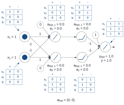
Figure 2: An expanded plot of the example XNOR NN from Figure 1 in the main paper, following the convention of separating linear and activation layers and showing the CAFE (1.0) attributions for the individual neurons.

Input Layer $L^{(1)}$

The first step of computing the CAFE explanation for this network is to evaluate the initial attribution scores for the neurons in the input layer $L^{(1)}$. Considering the differences between the features in the actual input ${\bm{x}}=(1,1)$ and the features in the reference input ${\bm{x}}_{\text{ref}}=(0,0)$, we obtain:

$$S^{(1),+}_{1,1} =\max(1-0,0)=1$$

$$S^{(1),+}_{2,2} =\max(1-0,0)=1$$

with the other scores for the input layer trivially being zero.

Linear Layer $L^{(2)}$

Next, we can compute the attribution scores for the first linear layer $L^{(2)}$ by performing a modified forward pass through this layer, distinguishing between positive and negative scores in the process. We get the following scores:

$$S^{(2),+}_{1,1} =(\max({W}^{(2)}_{1,1},0)\cdot S^{(1),+}_{1,1}+\max(-{W}^{(2)}_{1,1},0)\cdot S^{(1),-}_{1,1})+(\max({W}^{(2)}_{2,1},0)\cdot S^{(1),+}_{1,2}+\max(-{W}^{(2)}_{2,1},0)\cdot S^{(1),-}_{1,2})$$

$$=(\max(1,0)\cdot 1+\max(-1,0)\cdot 0)+(\max(-1,0)\cdot 0+\max(1,0)\cdot 0)=1$$

$$S^{(2),-}_{2,1} =(\max(-{W}^{(2)}_{1,1},0)\cdot S^{(1),+}_{2,1}+\max({W}^{(2)}_{1,1},0)\cdot S^{(1),-}_{2,1})+(\max(-{W}^{(2)}_{2,1},0)\cdot S^{(1),+}_{2,2}+\max({W}^{(2)}_{2,1},0)\cdot S^{(1),-}_{2,2})$$

$$=(\max(-1,0)\cdot 0+\max(1,0)\cdot 0)+(\max(1,0)\cdot 1+\max(-1,0)\cdot 0)=1$$

$$S^{(2),-}_{1,2} =(\max(-{W}^{(2)}_{1,2},0)\cdot S^{(1),+}_{1,1}+\max({W}^{(2)}_{1,2},0)\cdot S^{(1),-}_{1,1})+(\max(-{W}^{(2)}_{2,2},0)\cdot S^{(1),+}_{1,2}+\max({W}^{(2)}_{2,2},0)\cdot S^{(1),-}_{1,2})$$

$$=(\max(1,0)\cdot 1+\max(-1,0)\cdot 0)+(\max(-1,0)\cdot 0+\max(1,0)\cdot 0)=1$$

$$S^{(2),+}_{2,2} =(\max({W}^{(2)}_{1,2},0)\cdot S^{(1),+}_{2,1}+\max(-{W}^{(2)}_{1,2},0)\cdot S^{(1),-}_{2,1})+(\max({W}^{(2)}_{2,2},0)\cdot S^{(1),+}_{2,2}+\max(-{W}^{(2)}_{2,2},0)\cdot S^{(1),-}_{2,2})$$

$$=(\max(-1,0)\cdot 0+\max(1,0)\cdot 0)+(\max(1,0)\cdot 1+\max(-1,0)\cdot 0)=1$$

with the other scores again being zero.

Activation Layer $L^{(3)}$

We now have to propagate the scores through the ReLU activation layer $L^{(3)}$. Note that, since ReLU is a simple piecewise-linear function and since we are computing our attribution scores with respect to the zero reference input ${\bm{x}}_{\text{ref}}=(0,0)$, many of the computations for the activation rule may seem to be unnecessarily complex. However, it will be easy to see the importance of our general rules once we move to the following example considering a NN with a GELU activation and a non-zero reference input.

As the first step of applying the activation rule, we compute the input effects at each of the two ReLU neurons:

$${e}^{(3),+}_{1} =S^{(2),+}_{\text{bias},1}+S^{(2),+}_{1,1}+S^{(2),+}_{2,1}=0+1+0=1$$

$${e}^{(3),-}_{1} =-(S^{(2),-}_{\text{bias},1}+S^{(2),-}_{1,1}+S^{(2),-}_{2,1})=-(0+0+1)=-1$$

$${e}^{(3),*}_{1} =1+(-1)=0$$

$${e}^{(3),+}_{2} =S^{(2),+}_{\text{bias},2}+S^{(2),+}_{1,2}+S^{(2),+}_{2,2}=0+0+1=1$$

$${e}^{(3),-}_{2} =-(S^{(2),-}_{\text{bias},2}+S^{(2),-}_{1,2}+S^{(2),-}_{2,2})=-(0+1+0)=-1$$

$${e}^{(3),*}_{2} =1+(-1)=0$$

As we can observe, the input effects capture the fact that the two input features could cause the ReLU neuron pre-activation to change by $+1/-1$ compared to the reference input, but these influences completely cancelled out. Further following the procedure for the activation rule, we can now compute the rectified activation deltas. Recall that this is a three-stage process, starting with the computation of the activation function values at four points of interest:

$${a}^{(3),+}_{1} =\text{ReLU}({a}^{(2)}_{\text{ref},1}+{e}^{(3),+}_{1})=\text{ReLU}(0+1)=1$$

$${a}^{(3),-}_{1} =\text{ReLU}({a}^{(2)}_{\text{ref},1}+{e}^{(3),-}_{1})=\text{ReLU}(0+(-1))=0$$

$${a}^{(3),*}_{1} =\text{ReLU}({a}^{(2)}_{\text{ref},1}+{e}^{(3),*}_{1})=\text{ReLU}(0+0)=0$$

$${a}^{(3),\text{ref}}_{1} ={a}^{(3)}_{\text{ref},1}=\text{ReLU}({a}^{(2)}_{\text{ref},1})=\text{ReLU}(0)=0$$

In this and many of the following steps, we only show the computations for the first of the two ReLU neurons. This is because most of the intermediate values are exactly the same for both neurons, since the corresponding reference pre-activations and input effects are identical (although the scores for the individual features differ). We can now compute the auxiliary rectified activation deltas required for computing the final rectified activation deltas:

$$\Delta^{(3),(\text{ref}\rightarrow*),\nearrow}_{1} =\max({a}^{(3),*}_{1}-{a}^{(3),\text{ref}}_{1},0)=\max(0-0,0)=0$$

$$\Delta^{(3),(*\rightarrow+),\nearrow}_{1} =\max({a}^{(3),+}_{1}-{a}^{(3),*}_{1},0)=\max(1-0,0)=1$$

$$\Delta^{(3),(-\rightarrow\text{ref}),\nearrow}_{1} =\max({a}^{(3),\text{ref}}_{1}-{a}^{(3),-}_{1},0)=\max(0-0,0)=0$$

As before, we only show the steps for computing the deltas for the first ReLU neuron, with the deltas for the second neuron being identical. We also omit the auxiliary activation deltas that are zero or irrelevant to the subsequent steps. Using the quantities above, we can easily obtain the final rectified activation deltas:

$$\Delta^{(3),*,\nearrow}_{1} =\Delta^{(3),(\text{ref}\rightarrow*),\nearrow}_{1}=0$$

$$\Delta^{(3),+,\nearrow}_{1} =\Delta^{(3),(*\rightarrow+),\nearrow}_{1}=1$$

$$\Delta^{(3),-,\nearrow}_{1} =\Delta^{(3),(-\rightarrow\text{ref}),\nearrow}_{1}=0$$

Note that we only explicitly computed the deltas for a positive slope ($\nearrow$). Since the ReLU function is non-decreasing along its whole domain, the corresponding deltas for a negative slope ($\searrow$) are trivially zero. We can observe that the rectified activation deltas capture the fact that the activation function value did not change when considering the combined positive and negative inputs to the given neuron ($\Delta^{(3),*,\nearrow}_{1}=0$) or the negative inputs ($\Delta^{(3),-,\nearrow}_{1}=0$). However, it did increase by $1$ when considering only the positive inputs ($\Delta^{(3),+,\nearrow}_{1}=1$). We can now use the computed rectified activation deltas to evaluate the peak attribution flows:

$$p^{(3),(+\rightarrow+)}_{1} =\mathds{1}[{e}^{(3),*}_{1}\geq 0]\Delta^{(3),*,\nearrow}_{1}+\max(\Delta^{(3),+,\nearrow}_{1},\Delta^{(3),-,\nearrow}_{1})=1\cdot 0+\max(1,0)=1$$

$$p^{(3),(-\rightarrow+)}_{1} =\mathds{1}[-{e}^{(3),*}_{1}\geq 0]\Delta^{(3),*,\searrow}_{1}+\max(\Delta^{(3),+,\searrow}_{1},\Delta^{(3),-,\searrow}_{1})=1\cdot 0+\max(0,0)=0$$

$$p^{(3),(+\rightarrow-)}_{1} =\mathds{1}[{e}^{(3),*}_{1}\geq 0]\Delta^{(3),*,\searrow}_{1}+\max(\Delta^{(3),+,\searrow}_{1},\Delta^{(3),-,\searrow}_{1})=1\cdot 0+\max(0,0)=0$$

$$p^{(3),(-\rightarrow-)}_{1} =\mathds{1}[-{e}^{(3),*}_{1}\geq 0]\Delta^{(3),*,\nearrow}_{1}+\max(\Delta^{(3),+,\nearrow}_{1},\Delta^{(3),-,\nearrow}_{1})=1\cdot 0+\max(1,0)=1$$

As the peak attribution flows tell us, the positive inputs to the first ReLU neuron could increase its output by $1$, while the negative inputs could decrease its output by $1$. Since we are using the cancellation sensitivity constant value of $c^{(3)}=1$, we could theoretically skip the computation of the clipped linear attribution flows, as it does not influence the output scores in any way. Nevertheless, we include it for completeness:

$$l^{(3),(+\rightarrow+)}_{1} =\min\biggl{(}|{e}^{(3),+}_{1}|\frac{\Delta^{(3),*,\nearrow}_{1}}{|{e}^{(3),*}_{1}|+\epsilon},p^{(3),(+\rightarrow+)}_{1}\biggr{)}=\min\biggl{(}|1|\frac{0}{|0|+\epsilon},1\biggr{)}=\min(0,1)=0$$

$$l^{(3),(-\rightarrow+)}_{1} =\min\biggl{(}|{e}^{(3),-}_{1}|\frac{\Delta^{(3),*,\searrow}_{1}}{|{e}^{(3),*}_{1}|+\epsilon},p^{(3),(-\rightarrow+)}_{1}\biggr{)}=\min\biggl{(}|-1|\frac{0}{|0|+\epsilon},0\biggr{)}=\min(0,0)=0$$

$$l^{(3),(+\rightarrow-)}_{1} =\min\biggl{(}|{e}^{(3),+}_{1}|\frac{\Delta^{(3),*,\searrow}_{1}}{|{e}^{(3),*}_{1}|+\epsilon},p^{(3),(+\rightarrow-)}_{1}\biggr{)}=\min\biggl{(}|1|\frac{0}{|0|+\epsilon},0\biggr{)}=\min(0,0)=0$$

$$l^{(3),(-\rightarrow-)}_{1} =\min\biggl{(}|{e}^{(3),-}_{1}|\frac{\Delta^{(3),*,\nearrow}_{1}}{|{e}^{(3),*}_{1}|+\epsilon},p^{(3),(-\rightarrow-)}_{1}\biggr{)}=\min\biggl{(}|-1|\frac{0}{|0|+\epsilon},1\biggr{)}=\min(0,1)=0$$

As we can see, since there is no actually observed impact of the neuron inputs on its outputs (due to the conflicting features cancelling each other out), the linear attribution flows are all zero. We can now compute the attribution multipliers, the last intermediate quantity we need for obtaining the final scores:

$$m^{(3),(+\rightarrow+)}_{1} =\frac{(1-c^{(3)})l^{(3),(+\rightarrow+)}_{1}+c^{(3)}p^{(3),(+\rightarrow+)}_{1}}{|{e}^{(3),+}_{1}|+\epsilon}=\frac{(1-1)\cdot 0+1\cdot 1}{|1|+\epsilon}=1$$

$$m^{(3),(-\rightarrow+)}_{1} =\frac{(1-c^{(3)})l^{(3),(-\rightarrow+)}_{1}+c^{(3)}p^{(3),(-\rightarrow+)}_{1}}{|{e}^{(3),-}_{1}|+\epsilon}=\frac{(1-1)\cdot 0+1\cdot 0}{|-1|+\epsilon}=0$$

$$m^{(3),(+\rightarrow-)}_{1} =\frac{(1-c^{(3)})l^{(3),(+\rightarrow-)}_{1}+c^{(3)}p^{(3),(+\rightarrow-)}_{1}}{|{e}^{(3),+}_{1}|+\epsilon}=\frac{(1-1)\cdot 0+1\cdot 0}{|1|+\epsilon}=0$$

$$m^{(3),(-\rightarrow-)}_{1} =\frac{(1-c^{(3)})l^{(3),(-\rightarrow-)}_{1}+c^{(3)}p^{(3),(-\rightarrow-)}_{1}}{|{e}^{(3),-}_{1}|+\epsilon}=\frac{(1-1)\cdot 0+1\cdot 1}{|-1|+\epsilon}=1$$

In the above, we assumed that the value of $\epsilon$ is negligible. Given these multipliers, it is easy to see that the positive and negative attribution scores will actually stay the same when propagated through the ReLU layer. Indeed, for the final attribution scores, we obtain:

$$S^{(3),+}_{1,1} =m^{(3),(+\rightarrow+)}_{1}S^{(2),+}_{1,1}+m^{(3),(-\rightarrow+)}_{1}S^{(2),-}_{1,1}=1\cdot 1+0\cdot 0=1$$

$$S^{(3),-}_{2,1} =m^{(3),(+\rightarrow-)}_{1}S^{(2),+}_{2,1}+m^{(3),(-\rightarrow-)}_{1}S^{(2),-}_{2,1}=0\cdot 0+1\cdot 1=1$$

$$S^{(3),-}_{1,2} =m^{(3),(+\rightarrow-)}_{2}S^{(2),+}_{1,2}+m^{(3),(-\rightarrow-)}_{2}S^{(2),-}_{1,2}=0\cdot 0+1\cdot 1=1$$

$$S^{(3),+}_{2,2} =m^{(3),(+\rightarrow+)}_{2}S^{(2),+}_{2,2}+m^{(3),(-\rightarrow+)}_{2}S^{(2),-}_{2,2}=1\cdot 1+0\cdot 0=1$$

This time, we included the scores for the second ReLU neuron, as they differ from the first neuron, although we omitted the computation for scores evaluating to zero.

Linear Layer $L^{(4)}$

To obtain the final scores, we propagate the attributions through the linear layer $L^{(4)}$:

$$S^{(4),+}_{1,1} =(\max({W}^{(4)}_{1,1},0)\cdot S^{(3),+}_{1,1}+\max(-{W}^{(4)}_{1,1},0)\cdot S^{(3),-}_{1,1})+(\max({W}^{(4)}_{2,1},0)\cdot S^{(3),+}_{1,2}+\max(-{W}^{(4)}_{2,1},0)\cdot S^{(3),-}_{1,2})$$

$$=(\max(-1,0)\cdot 1+\max(1,0)\cdot 0)+(\max(-1,0)\cdot 0+\max(1,0)\cdot 1)=1$$

$$S^{(4),-}_{1,1} =(\max(-{W}^{(4)}_{1,1},0)\cdot S^{(3),+}_{1,1}+\max({W}^{(4)}_{1,1},0)\cdot S^{(3),-}_{1,1})+(\max(-{W}^{(4)}_{2,1},0)\cdot S^{(3),+}_{1,2}+\max({W}^{(4)}_{2,1},0)\cdot S^{(3),-}_{1,2})$$

$$=(\max(1,0)\cdot 1+\max(-1,0)\cdot 0)+(\max(1,0)\cdot 0+\max(-1,0)\cdot 1)=1$$

$$S^{(4),+}_{2,1} =(\max({W}^{(4)}_{1,1},0)\cdot S^{(3),+}_{2,1}+\max(-{W}^{(4)}_{1,1},0)\cdot S^{(3),-}_{2,1})+(\max({W}^{(4)}_{2,1},0)\cdot S^{(3),+}_{2,2}+\max(-{W}^{(4)}_{2,1},0)\cdot S^{(3),-}_{2,2})$$

$$=(\max(-1,0)\cdot 0+\max(1,0)\cdot 1)+(\max(-1,0)\cdot 1+\max(1,0)\cdot 0)=1$$

$$S^{(4),-}_{2,1} =(\max(-{W}^{(4)}_{1,1},0)\cdot S^{(3),+}_{2,1}+\max({W}^{(4)}_{1,1},0)\cdot S^{(3),-}_{2,1})+(\max(-{W}^{(4)}_{2,1},0)\cdot S^{(3),+}_{2,2}+\max({W}^{(4)}_{2,1},0)\cdot S^{(3),-}_{2,2})$$

$$=(\max(1,0)\cdot 0+\max(-1,0)\cdot 1)+(\max(1,0)\cdot 1+\max(-1,0)\cdot 0)=1$$

$$S^{(4),+}_{\text{bias},1} =(\max({W}^{(4)}_{1,1},0)\cdot S^{(3),+}_{\text{bias},1}+\max(-{W}^{(4)}_{1,1},0)\cdot S^{(3),-}_{\text{bias},1})+(\max({W}^{(4)}_{2,1},0)\cdot S^{(3),+}_{\text{bias},2}+\max(-{W}^{(4)}_{2,1},0)\cdot S^{(3),-}_{\text{bias},2})$$

$$\phantom{=(}+\max({b}^{(4)}_{1},0)=(\max(-1,0)\cdot 0+\max(1,0)\cdot 0)+(\max(-1,0)\cdot 0+\max(1,0)\cdot 0)+\max(1,0)=1$$

$$S^{(4),-}_{\text{bias},1} =(\max(-{W}^{(4)}_{1,1},0)\cdot S^{(3),+}_{\text{bias},1}+\max({W}^{(4)}_{1,1},0)\cdot S^{(3),-}_{\text{bias},1})+(\max(-{W}^{(4)}_{2,1},0)\cdot S^{(3),+}_{\text{bias},2}+\max({W}^{(4)}_{2,1},0)\cdot S^{(3),-}_{\text{bias},2})$$

$$\phantom{=(}+\max(-{b}^{(4)}_{1},0)=(\max(1,0)\cdot 0+\max(-1,0)\cdot 0)+(\max(1,0)\cdot 0+\max(-1,0)\cdot 0)+\max(-1,1)=0$$

As we can see, the scores capture the hypothetical impact of both conflicting features as well as the effect of the bias term.

C.2 GELU NN

In our second example, we will compute the CAFE (1.0) scores for the GELU NN from Figure 1 in the main text. As previously for the XNOR network from Section C.1, we provide a detailed visualisation of this network in Figure 3.

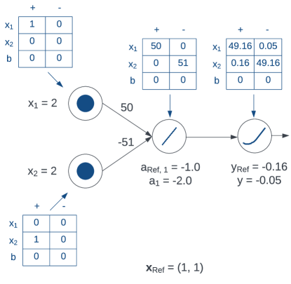
Figure 3: An expanded plot of the example GELU NN from Figure 1 in the main paper, following the convention of separating linear and activation layers and showing the CAFE (1.0) attributions for the individual neurons.

Input Layer $L^{(1)}$

We start by computing the attribution scores for the neurons in the input layer $L^{(1)}$. This can be done by considering the differences between the features in the actual input ${\bm{x}}=(2,2)$ and the features in the reference input ${\bm{x}}_{\text{ref}}=(2,2)$:

$$S^{(1),+}_{1,1} =\max(2-1,0)=1$$

$$S^{(1),+}_{2,2} =\max(2-1,0)=1$$

with all other scores being zero.

Linear Layer $L^{(2)}$

We proceed by propagating the scores through the first linear layer $L^{(2)}$, using our modified version of the standard forward pass:

$$S^{(2),+}_{1,1} =(\max({W}^{(2)}_{1,1},0)\cdot S^{(1),+}_{1,1}+\max(-{W}^{(2)}_{1,1},0)\cdot S^{(1),-}_{1,1})+(\max({W}^{(2)}_{2,1},0)\cdot S^{(1),+}_{1,2}+\max(-{W}^{(2)}_{2,1},0)\cdot S^{(1),-}_{1,2})$$

$$=(\max(50,0)\cdot 1+\max(-50,0)\cdot 0)+(\max(-51,0)\cdot 0+\max(51,0)\cdot 0)=50$$

$$S^{(2),-}_{2,1} =(\max(-{W}^{(2)}_{1,1},0)\cdot S^{(1),+}_{2,1}+\max({W}^{(2)}_{1,1},0)\cdot S^{(1),-}_{2,1})+(\max(-{W}^{(2)}_{2,1},0)\cdot S^{(1),+}_{2,2}+\max({W}^{(2)}_{2,1},0)\cdot S^{(1),-}_{2,2})$$

$$=(\max(-50,0)\cdot 0+\max(50,0)\cdot 0)+(\max(51,0)\cdot 1+\max(-51,0)\cdot 0)=51$$

As for the input layer, we only explicitly state the non-zero scores.

Activation Layer $L^{(3)}$

To obtain the final attribution scores, we apply the activation rule to the output GELU layer $L^{(3)}$. In contrast with the ReLU activations used in the XNOR example, the GELU function is non-monotonic, which will allow us to nicely illustrate the utility of the different auxiliary notions that we defined for the activation rule.

We start by computing the input effects at the output GELU neuron:

$${e}^{(3),+}_{1} =S^{(2),+}_{\text{bias},1}+S^{(2),+}_{1,1}+S^{(2),+}_{2,1}=0+50+0=50$$

$${e}^{(3),-}_{1} =-(S^{(2),-}_{\text{bias},1}+S^{(2),-}_{1,1}+S^{(2),-}_{2,1})=-(0+0+51)=-51$$

$${e}^{(3),*}_{1} =50+(-51)=-1$$

The values indicate that the positively contributing features (in this case, only $x_{1}$) could potentially increase the pre-activation of the GELU neuron by $50$ while the negative features ($x_{2}$) could decrease it by $51$. Taken together, the positive and negative features decrease the neuron pre-activation by $-1$.

Using the above values for the input effects, we can now compute the rectified activation deltas. As a first step of this three-stage process, we compute the activation function values at four points of interest:

$${a}^{(3),+}_{1} =\text{GELU}({a}^{(2)}_{\text{ref},1}+{e}^{(3),+}_{1})=\text{GELU}(-1+50)=49$$

$${a}^{(3),-}_{1} =\text{GELU}({a}^{(2)}_{\text{ref},1}+{e}^{(3),-}_{1})=\text{GELU}(-1+(-51))=0$$

$${a}^{(3),*}_{1} =\text{GELU}({a}^{(2)}_{\text{ref},1}+{e}^{(3),*}_{1})=\text{GELU}(-1+(-1))=-0.05$$

$${a}^{(3),\text{ref}}_{1} ={a}^{(3)}_{\text{ref},1}=\text{GELU}({a}^{(2)}_{\text{ref},1})=\text{GELU}(-1)=-0.16$$

We can now compute the auxiliary rectified activation deltas:

$$\Delta^{(3),(*\rightarrow\text{ref}),\searrow}_{1} =\max({a}^{(3),*}_{1}-{a}^{(3),\text{ref}}_{1},0)=\max(-0.05-(-0.16),0)=0.11$$

$$\Delta^{(3),(\text{ref}\rightarrow+),\nearrow}_{1} =\max({a}^{(3),+}_{1}-{a}^{(3),\text{ref}}_{1},0)=\max(49-(-0.16),0)=49.16$$

$$\Delta^{(3),(-\rightarrow*),\searrow}_{1} =\max({a}^{(3),-}_{1}-{a}^{(3),*}_{1},0)=\max(0-(-0.05),0)=0.05$$

Note that we omitted the auxiliary deltas that are zero or irrelevant to the subsequent steps. Using the computed values, we can directly obtain the final rectified activation deltas:

$$\Delta^{(3),*,\searrow}_{1} =\Delta^{(3),(*\rightarrow\text{ref}),\searrow}_{1}=0.11$$

$$\Delta^{(3),+,\nearrow}_{1} =\Delta^{(3),(\text{ref}\rightarrow+),\nearrow}_{1}=49.16$$

$$\Delta^{(3),-,\searrow}_{1} =\Delta^{(3),(-\rightarrow*),\searrow}_{1}=0.05$$

Before moving on, let us consider the meaning of the deltas we just computed. The rectified activation delta for the combined effect $\Delta^{(3),*,\searrow}_{1}$ tells us that the activation function decreased by $0.11$ on the interval between the reference pre-activation and the actual pre-activation for the currently observed input. This means that the actual inputs of the neuron changed its activation by $0.11$ with the function slope being negative on the corresponding interval. Meanwhile, the rectified activation delta for the positive effect $\Delta^{(3),+,\nearrow}_{1}$ indicates that the activation function increased by $49.16$ on an interval between the reference pre-activation and the pre-activation obtained by only considering the positively contributing inputs at the given neuron while disregarding the negative ones. This means that the activation of the neuron could potentially change by $49.16$ were it not for the negative features inhibiting this change. Finally, the rectified activation delta for the negative effect $\Delta^{(3),-,\searrow}_{1}$ signifies that the activation function decreased by $0.05$ on the interval between the pre-activation obtained by only considering the negatively contributing inputs and the actual pre-activation for the currently observed input. This tells us that the negative features on their own could further change the neuron output by $0.05$.

We can now use the computed rectified activation deltas to evaluate the peak attribution flows:

$$p^{(3),(+\rightarrow+)}_{1} =\mathds{1}[{e}^{(3),*}_{1}\geq 0]\Delta^{(3),*,\nearrow}_{1}+\max(\Delta^{(3),+,\nearrow}_{1},\Delta^{(3),-,\nearrow}_{1})=0\cdot 0+\max(49.16,0)=49.16$$

$$p^{(3),(-\rightarrow+)}_{1} =\mathds{1}[-{e}^{(3),*}_{1}\geq 0]\Delta^{(3),*,\searrow}_{1}+\max(\Delta^{(3),+,\searrow}_{1},\Delta^{(3),-,\searrow}_{1})=1\cdot 0.11+\max(0,0.05)=0.16$$

$$p^{(3),(+\rightarrow-)}_{1} =\mathds{1}[{e}^{(3),*}_{1}\geq 0]\Delta^{(3),*,\searrow}_{1}+\max(\Delta^{(3),+,\searrow}_{1},\Delta^{(3),-,\searrow}_{1})=0\cdot 0.11+\max(0,0.05)=0.05$$

$$p^{(3),(-\rightarrow-)}_{1} =\mathds{1}[-{e}^{(3),*}_{1}\geq 0]\Delta^{(3),*,\nearrow}_{1}+\max(\Delta^{(3),+,\nearrow}_{1},\Delta^{(3),-,\nearrow}_{1})=1\cdot 0+\max(49.16,0)=49.16$$

As we can see, the peak attribution flows capture the possible effects of the positive/negative inputs on the positive/negative outputs of the given GELU neuron. In particular, the positive inputs can be seen as potentially increasing the output of the neuron by 49.16 from the reference output value, while the negative inputs can be seen as counteracting this by decreasing it by the same value. However, as the GELU function is non-monotonic, positive inputs can also be seen as causing a decrease in the output of the neuron by 0.05, which is caused by preventing the negative features from pushing the pre-activation to a range in which the GELU function is zero instead of being negative. Meanwhile, the negative inputs can also be seen as causing an increase in the output of the neuron by 0.16, by pushing the pre-activation further away from the global GELU minimum.

For reference, we also compute the clipped linear attribution flows, even though they are not strictly needed when using the conflict sensitivity constant $c^{(3)}=1$:

$$l^{(3),(+\rightarrow+)}_{1} =\min\biggl{(}|{e}^{(3),+}_{1}|\frac{\Delta^{(3),*,\nearrow}_{1}}{|{e}^{(3),*}_{1}|+\epsilon},p^{(3),(+\rightarrow+)}_{1}\biggr{)}=\min\biggl{(}|50|\frac{0}{|-1|+\epsilon},49.16\biggr{)}=\min(0,49.16)=0$$

$$l^{(3),(-\rightarrow+)}_{1} =\min\biggl{(}|{e}^{(3),-}_{1}|\frac{\Delta^{(3),*,\searrow}_{1}}{|{e}^{(3),*}_{1}|+\epsilon},p^{(3),(-\rightarrow+)}_{1}\biggr{)}=\min\biggl{(}|-51|\frac{0.11}{|-1|+\epsilon},0.16\biggr{)}=\min(5.61,0.16)=0.16$$

$$l^{(3),(+\rightarrow-)}_{1} =\min\biggl{(}|{e}^{(3),+}_{1}|\frac{\Delta^{(3),*,\searrow}_{1}}{|{e}^{(3),*}_{1}|+\epsilon},p^{(3),(+\rightarrow-)}_{1}\biggr{)}=\min\biggl{(}|50|\frac{0.11}{|-1|+\epsilon},0.05\biggr{)}=\min(5.5,0.05)=0.05$$

$$l^{(3),(-\rightarrow-)}_{1} =\min\biggl{(}|{e}^{(3),-}_{1}|\frac{\Delta^{(3),*,\nearrow}_{1}}{|{e}^{(3),*}_{1}|+\epsilon},p^{(3),(-\rightarrow-)}_{1}\biggr{)}=\min\biggl{(}|-51|\frac{0}{|-1|+\epsilon},49.16\biggr{)}=\min(0,49.16)=0$$

As we can observe, clipping the scores with the values of peak attribution flows prevented the attribution score explosion issue in this case, as the linear approximation on its own grossly overestimated the possible effects of the neuron inputs. Indeed, since the GELU function flattens and tends to 0 as its input becomes increasingly negative, the highest amount by which the negative inputs can increase the output from the reference value $y_{\text{ref}}=-0.16$ is 0.16 — much lower than the estimated value of 5.61.

We are now in position to compute the attribution multipliers needed for obtaining the final scores:

$$m^{(3),(+\rightarrow+)}_{1} =\frac{(1-c^{(3)})l^{(3),(+\rightarrow+)}_{1}+c^{(3)}p^{(3),(+\rightarrow+)}_{1}}{|{e}^{(3),+}_{1}|+\epsilon}=\frac{(1-1)\cdot 0+1\cdot 49.16}{|50|+\epsilon}=0.9832$$

$$m^{(3),(-\rightarrow+)}_{1} =\frac{(1-c^{(3)})l^{(3),(-\rightarrow+)}_{1}+c^{(3)}p^{(3),(-\rightarrow+)}_{1}}{|{e}^{(3),-}_{1}|+\epsilon}=\frac{(1-1)\cdot 0.16+1\cdot 0.16}{|-51|+\epsilon}=0.0031$$

$$m^{(3),(+\rightarrow-)}_{1} =\frac{(1-c^{(3)})l^{(3),(+\rightarrow-)}_{1}+c^{(3)}p^{(3),(+\rightarrow-)}_{1}}{|{e}^{(3),+}_{1}|+\epsilon}=\frac{(1-1)\cdot 0.05+1\cdot 0.05}{|50|+\epsilon}=0.0010$$

$$m^{(3),(-\rightarrow-)}_{1} =\frac{(1-c^{(3)})l^{(3),(-\rightarrow-)}_{1}+c^{(3)}p^{(3),(-\rightarrow-)}_{1}}{|{e}^{(3),-}_{1}|+\epsilon}=\frac{(1-1)\cdot 0+1\cdot 49.16}{|-51|+\epsilon}=0.9639$$

Note that the multipliers are normalised by the positive/negative effect values at the given neuron. In this example, this is not strictly needed, as it only involves a single positively contributing feature and a single negatively contributing feature to the pre-activation of the considered GELU neuron. However, in general, there could be multiple such features, requiring us to distribute the total scores between them proportionally to their impact on the neuron pre-activations.

Given the multipliers above, we can now easily compute the final attribution scores:

$$S^{(3),+}_{1,1} =m^{(3),(+\rightarrow+)}_{1}S^{(2),+}_{1,1}+m^{(3),(-\rightarrow+)}_{1}S^{(2),-}_{1,1}=0.9832\cdot 50+0.0031\cdot 0=49.16$$

$$S^{(3),-}_{1,1} =m^{(3),(+\rightarrow-)}_{1}S^{(2),+}_{1,1}+m^{(3),(-\rightarrow-)}_{1}S^{(2),-}_{1,1}=0.0010\cdot 50+0.9639\cdot 0=0.05$$

$$S^{(3),+}_{2,1} =m^{(3),(+\rightarrow+)}_{1}S^{(2),+}_{2,1}+m^{(3),(-\rightarrow+)}_{1}S^{(2),-}_{2,1}=0.9832\cdot 0+0.0031\cdot 51=0.16$$

$$S^{(3),-}_{2,1} =m^{(3),(+\rightarrow-)}_{1}S^{(2),+}_{2,1}+m^{(3),(-\rightarrow-)}_{1}S^{(2),-}_{2,1}=0.0010\cdot 0+0.9639\cdot 51=49.16$$

As we can see, the scores directly match those shown in the Figure above, as well as those stated in the corresponding table in Figure 1 of the main paper.

C.3 GELU Neuron Visualisation

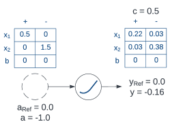
Figure 4: The example GELU neuron considered in Section 5. We assume that we already computed the attribution scores for the neuron pre-activation, which are visualised in the figure.

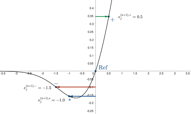
Figure 5: Visualisation of the input effects for the example GELU neuron

To provide further intuition regarding the activation rule, we consider one more example. This time, we will only consider propagating the CAFE (0.5) attribution scores through a single GELU neuron, allowing us to provide a more comprehensive visualisation of the whole process. The considered neuron is shown in Figure 4. Note that we assume that we have already computed the attribution scores for the neuron pre-activations: $S^{(n),+}_{1,j}=0.5$ and $S^{(n),-}_{2,j}=1.5$ with the other scores being zero, as visualised in the figure.

As in the previous applications of the activation rule, we start by computing the input effects at the neuron:

$${e}^{(n+1),+}_{j} =S^{(n),+}_{\text{bias},j}+S^{(n),+}_{1,j}+S^{(n),+}_{2,j}=0+0.5+0=0.5$$

$${e}^{(n+1),-}_{j} =-(S^{(n),-}_{\text{bias},j}+S^{(n),-}_{1,j}+S^{(n),-}_{2,j})=-(0+0+1.5)=-1.5$$

$${e}^{(n+1),*}_{j} =0.5+(-1.5)=-1$$

For illustration, these effects are also visualised in Figure 5.

We can now compute the rectified activation deltas. As in the previous examples, we follow a three-stage procedure, starting by computing the activation function values at four points of interest:

$${a}^{(n+1),+}_{j} =\text{GELU}({a}^{(n)}_{\text{ref},j}+{e}^{(n+1),+}_{j})=\text{GELU}(0+0.5)=0.35$$

$${a}^{(n+1),-}_{j} =\text{GELU}({a}^{(n)}_{\text{ref},j}+{e}^{(n+1),-}_{j})=\text{GELU}(0+(-1.5))=-0.10$$

$${a}^{(n+1),*}_{j} =\text{GELU}({a}^{(n)}_{\text{ref},j}+{e}^{(n+1),*}_{j})=\text{GELU}(0+(-0.5))=-0.16$$

$${a}^{(n+1),\text{ref}}_{j} ={a}^{(n+1)}_{\text{ref},j}=\text{GELU}({a}^{(n)}_{\text{ref},j})=\text{GELU}(0)=0$$

We proceed by computing the auxiliary rectified activation deltas:

$$\Delta^{(n+1),(*\rightarrow\text{ref}),\nearrow}_{j} =\max({a}^{(n+1),\text{ref}}_{j}-{a}^{(n+1),*}_{j},0)=\max(0-(-0.16),0)=0.16$$

$$\Delta^{(n+1),(\text{ref}\rightarrow+),\nearrow}_{j} =\max({a}^{(n+1),+}_{j}-{a}^{(n+1),\text{ref}}_{j},0)=\max(0.35-0,0)=0.35$$

$$\Delta^{(n+1),(-\rightarrow*),\searrow}_{j} =\max({a}^{(n+1),-}_{j}-{a}^{(n+1),*}_{j},0)=\max(-0.10-(-0.16),0)=0.06$$

Finally, we can obtain the main rectified activation deltas:

$$\Delta^{(n+1),*,\nearrow}_{j} =\Delta^{(n+1),(\text{ref}\rightarrow*),\nearrow}_{j}=0.16$$

$$\Delta^{(n+1),+,\nearrow}_{j} =\Delta^{(n+1),(\text{ref}\rightarrow+),\nearrow}_{j}=0.35$$

$$\Delta^{(n+1),-,\searrow}_{j} =\Delta^{(n+1),(-\rightarrow*),\searrow}_{j}=0.06$$

Note that in all the above steps, we only list non-zero deltas relevant to computing the attribution scores. We visualise the rectified activation deltas in Figure 6.

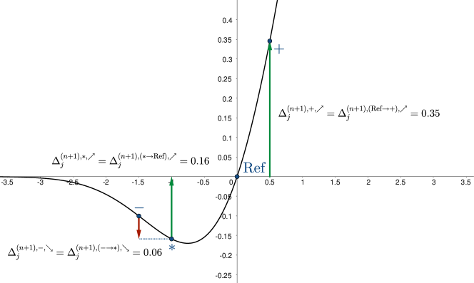
Figure 6: Visualisation of the rectified activation deltas for the example GELU neuron

With the rectified activation deltas above, we can now evaluate the peak attribution flows:

$$p^{(n+1),(+\rightarrow+)}_{j} =\mathds{j}[{e}^{(n+1),*}_{j}\geq 0]\Delta^{(n+1),*,\nearrow}_{j}+\max(\Delta^{(n+1),+,\nearrow}_{j},\Delta^{(n+1),-,\nearrow}_{j})=0\cdot 0.16+\max(0.35,0)=0.35$$

$$p^{(n+1),(-\rightarrow+)}_{j} =\mathds{j}[-{e}^{(n+1),*}_{j}\geq 0]\Delta^{(n+1),*,\searrow}_{j}+\max(\Delta^{(n+1),+,\searrow}_{j},\Delta^{(n+1),-,\searrow}_{j})=1\cdot 0+\max(0,0.06)=0.06$$

$$p^{(n+1),(+\rightarrow-)}_{j} =\mathds{j}[{e}^{(n+1),*}_{j}\geq 0]\Delta^{(n+1),*,\searrow}_{j}+\max(\Delta^{(n+1),+,\searrow}_{j},\Delta^{(n+1),-,\searrow}_{j})=0\cdot 0.11+\max(0,0.06)=0.06$$

$$p^{(n+1),(-\rightarrow-)}_{j} =\mathds{j}[-{e}^{(n+1),*}_{j}\geq 0]\Delta^{(n+1),*,\nearrow}_{j}+\max(\Delta^{(3),+,\nearrow}_{j},\Delta^{(n+1),-,\nearrow}_{j})=1\cdot 0.16+\max(0.35,0)=0.51$$

The key quantities used in the computation of the peak attribution flows are visualised in Figure 7. The two bidirectional arrows with lighter shades indicate the components capturing the “hypothetical”, cancelled effects of the inputs on the outputs. In order to maintain the completeness property, these are always added to the peak attribution flows with opposite targets, ensuring that they cancel out when subtracted from each other. Meanwhile, the dark-green unidirectional arrow indicates the “real” difference in the neuron output observed for the currently used input. This quantity is only added to one of the peak attribution flows with the corresponding target sign, in line with the completeness property.

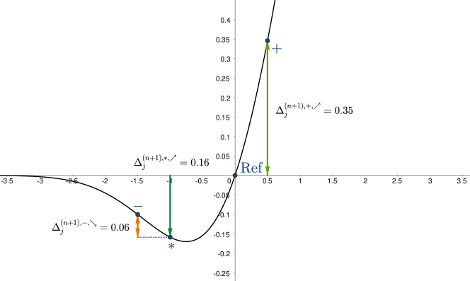
Figure 7: Visualisation of the key quantities used in the computation of the peak attribution flows for the example GELU neuron

We can now proceed by computing the clipped linear attribution flows:

$$l^{(n+1),(+\rightarrow+)}_{j} =\min\biggl{(}|{e}^{(n+1),+}_{j}|\frac{\Delta^{(n+1),*,\nearrow}_{j}}{|{e}^{(n+1),*}_{j}|+\epsilon},p^{(n+1),(+\rightarrow+)}_{j}\biggr{)}=\min\biggl{(}|0.5|\frac{0.16}{|-1|+\epsilon},0.35\biggr{)}=\min(0.08,0.35)=0.08$$

$$l^{(n+1),(-\rightarrow+)}_{j} =\min\biggl{(}|{e}^{(n+1),-}_{j}|\frac{\Delta^{(n+1),*,\searrow}_{j}}{|{e}^{(n+1),*}_{j}|+\epsilon},p^{(n+1),(-\rightarrow+)}_{j}\biggr{)}=\min\biggl{(}|-1.5|\frac{0}{|-1|+\epsilon},0.06\biggr{)}=\min(0,0.06)=0$$

$$l^{(n+1),(+\rightarrow-)}_{j} =\min\biggl{(}|{e}^{(n+1),+}_{j}|\frac{\Delta^{(n+1),*,\searrow}_{j}}{|{e}^{(n+1),*}_{j}|+\epsilon},p^{(n+1),(+\rightarrow-)}_{j}\biggr{)}=\min\biggl{(}|0.5|\frac{0}{|-1|+\epsilon},0.06\biggr{)}=\min(0,0.06)=0$$

$$l^{(n+1),(-\rightarrow-)}_{j} =\min\biggl{(}|{e}^{(n+1),-}_{j}|\frac{\Delta^{(n+1),*,\nearrow}_{j}}{|{e}^{(n+1),*}_{j}|+\epsilon},p^{(n+1),(-\rightarrow-)}_{j}\biggr{)}=\min\biggl{(}|-1.5|\frac{0.16}{|-1|+\epsilon},0.51\biggr{)}=\min(0.24,0.51)=0.24$$

The computation of clipped linear attribution flows is visualised in Figure 8. As we can observe, the main quantities used for computing the linear attribution flows are based on a linear approximation of the activation function between the reference pre-activation and the pre-activation for the current input. In this case, the linear approximation does not overestimate the possible outputs of the function, so the values obtained in this way can be used directly without being clipped by the values of the peak attribution flows.

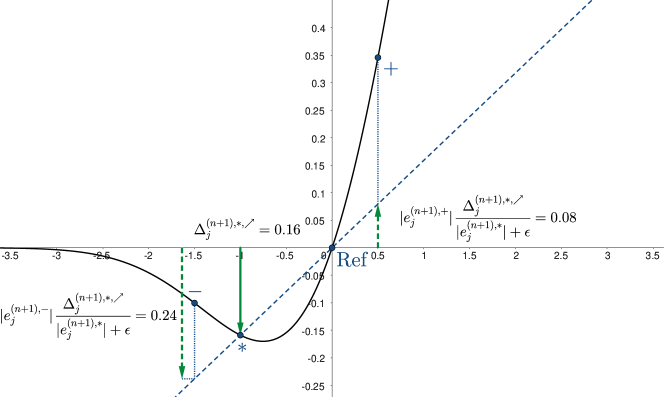
Figure 8: Visualisation of the computation of clipped linear attribution flows for the example GELU neuron

With the above peak attribution flows and clipped linear attribution flows, we can now compute the attribution multipliers:

$$m^{(n+1),(+\rightarrow+)}_{j} =\frac{(1-c^{(n+1)})l^{(n+1),(+\rightarrow+)}_{j}+c^{(n+1)}p^{(n+1),(+\rightarrow+)}_{j}}{|{e}^{(n+1),+}_{j}|+\epsilon}=\frac{(1-0.5)\cdot 0.08+0.5\cdot 0.35}{|0.5|+\epsilon}=0.43$$

$$m^{(n+1),(-\rightarrow+)}_{j} =\frac{(1-c^{(n+1)})l^{(n+1),(-\rightarrow+)}_{j}+c^{(n+1)}p^{(n+1),(-\rightarrow+)}_{j}}{|{e}^{(n+1),-}_{j}|+\epsilon}=\frac{(1-0.5)\cdot 0+0.5\cdot 0.06}{|-1.5|+\epsilon}=0.02$$

$$m^{(n+1),(+\rightarrow-)}_{j} =\frac{(1-c^{(n+1)})l^{(n+1),(+\rightarrow-)}_{j}+c^{(n+1)}p^{(n+1),(+\rightarrow-)}_{j}}{|{e}^{(n+1),+}_{j}|+\epsilon}=\frac{(1-0.5)\cdot 0+0.5\cdot 0.06}{|0.5|+\epsilon}=0.06$$

$$m^{(n+1),(-\rightarrow-)}_{j} =\frac{(1-c^{(n+1)})l^{(n+1),(-\rightarrow-)}_{j}+c^{(n+1)}p^{(n+1),(-\rightarrow-)}_{j}}{|{e}^{(n+1),-}_{j}|+\epsilon}=\frac{(1-0.5)\cdot 0.24+0.5\cdot 0.51}{|-1.5|+\epsilon}=0.25$$

Given these multipliers, we can now compute the final attribution scores:

$$S^{(n+1),+}_{1,j} =m^{(n+1),(+\rightarrow+)}_{j}S^{(n),+}_{1,j}+m^{(n+1),(-\rightarrow+)}_{j}S^{(n),-}_{1,j}=0.43\cdot 0.5+0.02\cdot 0=0.22$$

$$S^{(n+1),-}_{1,j} =m^{(n+1),(+\rightarrow-)}_{j}S^{(n),+}_{1,j}+m^{(n+1),(-\rightarrow-)}_{j}S^{(n),-}_{1,j}=0.06\cdot 0.5+0.25\cdot 0=0.03$$

$$S^{(n+1),+}_{2,j} =m^{(n+1),(+\rightarrow+)}_{j}S^{(n),+}_{2,j}+m^{(n+1),(-\rightarrow+)}_{j}S^{(n),-}_{2,j}=0.43\cdot 0+0.02\cdot 1.5=0.03$$

$$S^{(n+1),-}_{2,j} =m^{(n+1),(+\rightarrow-)}_{j}S^{(n),+}_{2,j}+m^{(n+1),(-\rightarrow-)}_{1}S^{(n),-}_{2,j}=0.06\cdot 0+0.25\cdot 1.5=0.38$$

Appendix D CAFE PROPERTIES AND PROOFS

In this section of the appendix, we provide detailed definitions and proofs of the theoretical properties introduced in Section 5.1 of the main text. We also give a more detailed analysis of the computational complexity of CAFE and compare its properties to other relevant methods.

D.1 Missingness

In this section, we show that CAFE satisfies the “missingness” property, which was previously considered by Lundberg and Lee, (2017) (though their version did not include reference inputs):

Property 1 (Missingness).

A feature attribution satisfies the missingness property iff the attribution method always assigns a score of $0$ to features:

1. that are $0$, if the feature attribution method does not use a reference input.

2. that are equal to the reference input, if the feature attribution method uses a reference input.

Proposition 1.

CAFE satisfies the missingness property for any choice of the constants $c^{(n)}$ for the individual layers.

Proof 1.

We prove Proposition 1 by structural induction over the CAFE rules.

For the base case, we aim to show that, for an arbitrary input ${\bm{x}}$, reference input ${\bm{x}}_{\text{ref}}$, input layer $L^{(1)}$, feature index $f$, we have $x_{\text{ref},f}=x_{f}\implies\forall i.[S^{(1),+}_{f,i}=0\land S^{(1),-}_{f,i}=0]$. Assuming $x_{\text{ref},f}=x_{f}$ and taking an arbitrary $i$, we consider two cases:

1. $f=i$. Then, by the input layer rule,

   $$S^{(1),+}_{f,i} =\max(x_{f}-x_{\text{ref},f},0)=\max(x_{f}-x_{f},0)=\max(0,0)=0$$

   $$S^{(1),-}_{f,i} =\max(-(x_{f}-x_{\text{ref},f}))=\max(x_{f}-x_{f},0)=\max(0,0)=0$$

   as required.

2. $f\neq i$. Then, $S^{(1),+}_{f,i}=0$ and $S^{(1),-}_{f,i}=0$ directly, by definition.

Thus, we have shown that $\forall i.[S^{(1),+}_{f,i}=0\land S^{(1),-}_{f,i}=0]$ given the assumption $x_{\text{ref},f}=x_{f}$, which concludes the proof of the base case.

For the linear rule case, we aim to show that, for an arbitrary linear layer $L^{(n+1)}$ where $n\geq 1$ and feature index $f$, we have $x_{\text{ref},f}=x_{f}\implies\forall j.[S^{(n+1),+}_{f,i}=0\land S^{(n+1),-}_{f,i}=0]$, given the inductive hypothesis $x_{\text{ref},f}=x_{f}\implies\forall i.[S^{(n),+}_{f,i}=0\land S^{(n),-}_{f,i}=0]$. Assuming $x_{\text{ref},f}=x_{f}$, taking an arbitrary neuron index $j$ and applying the linear rule, we get:

$$S^{(n+1),+}_{f,j} =\sum_{i}^{|L^{(n)}|}\left(\max({W}^{(n+1)}_{i,j},0)\cdot S^{(n),+}_{f,i}+\max(-{W}^{(n+1)}_{i,j},0)\cdot S^{(n),-}_{f,i}\right)$$

$$=\sum_{i}^{|L^{(n)}|}\left(\max({W}^{(n+1)}_{i,j},0)\cdot 0+\max(-{W}^{(n+1)}_{i,j},0)\cdot 0\right)=0$$

$$S^{(n+1),-}_{f,j} =\sum_{i}^{|L^{(n)}|}\left(\max(-{W}^{(n+1)}_{i,j},0)\cdot S^{(n),+}_{f,i}+\max(-(-{W}^{(n+1)}_{i,j}),0)\cdot S^{(n),-}_{f,i}\right)$$

$$=\sum_{i}^{|L^{(n)}|}\left(\max(-{W}^{(n+1)}_{i,j},0)\cdot 0+\max({W}^{(n+1)}_{i,j},0)\cdot 0\right)=0$$

where the second step follows directly from the inductive hypothesis. This shows that $x_{\text{ref},f}=x_{f}\implies\forall j.[S^{(n+1),+}_{f,i}=0\land S^{(n+1),-}_{f,i}=0]$, concluding the proof of the linear rule case.

For the activation rule case, we aim to show that, for an arbitrary activation layer $L^{(n+1)}$ where $n\geq 1$ and feature index $f$, we have $x_{\text{ref},f}=x_{f}\implies\forall j.[S^{(n+1),+}_{f,j}=0\land S^{(n+1),-}_{f,j}=0]$, given the inductive hypothesis $x_{\text{ref},f}=x_{f}\implies\forall i.[S^{(n),+}_{f,i}=0\land S^{(n),-}_{f,i}=0]$. Assuming $x_{\text{ref},f}=x_{f}$, taking an arbitrary neuron index $j$ and applying the activation rule, we get:

$$S^{(n+1),+}_{f,j} =S^{(n),+}_{f,j}m^{(n+1),(+\rightarrow+)}_{j}+S^{(n),-}_{f,j}m^{(n+1),(-\rightarrow+)}_{j}$$

$$=0\cdot m^{(n+1),(+\rightarrow+)}_{j}+0\cdot m^{(n+1),(-\rightarrow+)}_{j}=0$$

$$S^{(n+1),-}_{f,j} =S^{(n),+}_{f,j}m^{(n+1),(+\rightarrow-)}_{j}+S^{(n),-}_{f,j}m^{(n+1),(-\rightarrow-)}_{j}$$

$$=0\cdot m^{(n+1),(+\rightarrow-)}_{j}+0\cdot m^{(n+1),(-\rightarrow-)}_{j}=0$$

where the second step again follows directly from the inductive hypothesis. This shows that $x_{\text{ref},f}=x_{f}\implies\forall i.[S^{(n),+}_{f,i}=0\land S^{(n),-}_{f,i}=0]$, concluding our proof for the activation rule.

Since we have considered all the CAFE rules, by induction, we have proven Proposition 1.

D.2 Linearity

As our next formal property, we consider linearity, which has been previously proposed as a desirable axiom for the Integrated Gradients method (Sundararajan et al.,, 2017):

Property 2 (Linearity).

A feature attribution method is linear iff, for any two models $\mathcal{M}_{1}$ and $\mathcal{M}_{2}$, coefficients $a$ and $b$, a combined model $\mathcal{M}_{3}({\bm{x}})\triangleq a\cdot\mathcal{M}_{1}({\bm{x}})+b\cdot\mathcal{M}_{2}({\bm{x}})$, current input ${\bm{x}}$ and reference input ${\bm{x}}_{\text{ref}}$ (if the attribution method takes a reference input), the feature attribution scores for $\mathcal{M}_{3}$ and input ${\bm{x}}$ with respect to the reference input ${\bm{x}}_{\text{ref}}$ are equal to ${\bm{S}}_{3}=a\cdot{\bm{S}}_{1}+b\cdot{\bm{S}}_{2}$, where ${\bm{S}}_{1}$ and ${\bm{S}}_{2}$ are the attribution scores computed for the input ${\bm{x}}$, reference input ${\bm{x}}_{\text{ref}}$ and the models $\mathcal{M}_{1}$ and $\mathcal{M}_{2}$, respectively.

Proposition 2.

CAFE is linear for any choice of the constants $c^{(n)}$ for the individual layers, considering the joint attribution scores ${\bm{S}}^{*}={\bm{S}}^{+}-{\bm{S}}^{-}$.

We restrict Proposition 2 to the joint feature attribution scores, as the linearity property was originally proposed for methods returning a single score for each feature.

Proof 2.

To prove Proposition 2, it is only sufficient to consider the linear rule, as the other rules do not apply when computing the scores for a linear combination of two inputs. Take arbitrary models $\mathcal{M}_{1}$ and $\mathcal{M}_{2}$, coefficients $a$ and $b$, a combined model such that $\mathcal{M}_{3}({\bm{x}})\triangleq a\cdot\mathcal{M}_{1}({\bm{x}})+b\cdot\mathcal{M}_{2}({\bm{x}})$, current input ${\bm{x}}$ and reference input ${\bm{x}}_{\text{ref}}$ (if the attribution method takes a reference input). We aim to show that, if CAFE returns scores ${\bm{S}}^{+}_{1}$ and ${\bm{S}}^{-}_{1}$ for $\mathcal{M}_{1}$, scores ${\bm{S}}^{+}_{2}$ and ${\bm{S}}^{-}_{2}$ for $\mathcal{M}_{2}$ and scores ${\bm{S}}^{+}_{3}$ and ${\bm{S}}^{-}_{3}$ (while considering the current input ${\bm{x}}$ and the reference input ${\bm{x}}_{\text{ref}}$), the following equality will hold: ${\bm{S}}^{+}_{3}-{\bm{S}}^{-}_{3}=a\cdot({\bm{S}}^{+}_{1}-{\bm{S}}^{-}_{1})+b\cdot({\bm{S}}^{+}_{2}-{\bm{S}}^{-}_{2})$. Since we only have two weights, $a$ and $b$, and no additive biases in the current linear operation, by the linear rule, we get:

$${\bm{S}}^{+}_{3}-{\bm{S}}^{-}_{3}$$

$$=\max(a,0)\cdot{\bm{S}}^{+}_{1}+\max(-a,0)\cdot{\bm{S}}^{-}_{1}+\max(b,0)\cdot{\bm{S}}^{+}_{2}+\max(-b,0)\cdot{\bm{S}}^{-}_{2}$$

$$\phantom{=(}-(\max(-a,0)\cdot{\bm{S}}^{+}_{1}+\max(-(-a),0)\cdot{\bm{S}}^{-}_{1}+\max(-b,0)\cdot{\bm{S}}^{+}_{2}+\max(-(-b),0)\cdot{\bm{S}}^{-}_{2})$$

$$=(\max(a,0)-\max(-a,0))\cdot({\bm{S}}^{+}_{1}-{\bm{S}}^{-}_{1})+(\max(b,0)-\max(-b,0))\cdot({\bm{S}}^{+}_{2}-{\bm{S}}^{-}_{2})$$

$$=a\cdot({\bm{S}}^{+}_{1}-{\bm{S}}^{-}_{1})+b\cdot({\bm{S}}^{+}_{2}-{\bm{S}}^{-}_{2})$$

as required. This concludes the proof.

D.3 Completeness

As our final property, we consider completeness, which has been previously considered by several as a desirable property for feature attribution methods (Sundararajan et al.,, 2017; Shrikumar et al.,, 2017; Ancona et al.,, 2018):

Property 3 (Completeness).

A feature attribution method is complete iff, for any model $\mathcal{M}$, input ${\bm{x}}$ and reference input ${\bm{x}}_{\text{ref}}$, for which the attribution method computes scores s:

1. $\mathcal{M}({\bm{x}})=\sum_{f}S_{f}$, i.e. the sum of all returned feature attribution scores is equal to the model output, if the feature attribution method does not use a reference input.

2. $\mathcal{M}({\bm{x}})-\mathcal{M}({\bm{x}}_{\text{ref}})=\sum_{f}S_{f}$, i.e. the sum of all returned feature attribution scores is equal to the difference between the model outputs for the input ${\bm{x}}$ and the reference input ${\bm{x}}_{\text{ref}}$, if the feature attribution method uses a reference input.

Intuitively, the completeness property states that the attribution method should exactly account for all the changes to the model output as a result of the model input or the differences between the current input and the reference input. For CAFE, we wish to show the following proposition:

Proposition 3.

CAFE satisfies the completeness property for any choice of the constants $c^{(n)}$ for the individual layers, provided that the negative feature attribution scores ${\bm{S}}^{-}$ are considered to be negative when summing the scores and that $\mathcal{M}_{\text{ref}}({\bm{x}}_{\text{ref}})$ is considered as the baseline output.

As previously with linearity, our proposition needs to specify the handling of the two different kinds of scores returned by CAFE, as the original property was formulated for attribution methods only computing a single score. Similarly, since CAFE additionally captures the effects of the biases, we adjust the proposition to consider the reference output from a model without such biases $\mathcal{M}_{\text{ref}}$.

Proof 3.

We prove Proposition 3 by structural induction over the CAFE rules.

For the base case, we aim to show that, for an arbitrary input ${\bm{x}}$, reference input ${\bm{x}}_{\text{ref}}$ and input layer $L^{(1)}$, we have $\forall i.[\sum_{f}S^{(1),+}_{f,i}+S^{(1),+}_{\text{bias},i}-\sum_{f}S^{(1),-}_{f,i}-S^{(1),-}_{\text{bias},i}=x_{f}-x_{\text{ref},f}]$. By taking an arbitrary $i$ and applying the input layer rule, we get:

$$\sum_{f}^{|\mathbf{x}|}S^{(1),+}_{f,i}+S^{(1),+}_{\text{bias},i}-\sum_{f}^{|\mathbf{x}|}S^{(1),-}_{f,i}-S^{(1),-}_{\text{bias},i}$$

$$=\sum_{f\neq i}^{|\mathbf{x}|}S^{(1),+}_{f,i}+S^{(1),+}_{i,i}+S^{(1),+}_{\text{bias},i}-\sum_{f\neq i}^{|\mathbf{x}|}S^{(1),-}_{f,i}-S^{(1),-}_{i,i}-S^{(1),-}_{\text{bias},i}$$

$$=0+\max(x_{f}-x_{\text{ref},f},0)+0-0-\max(x_{\text{ref},f}-x_{f},0)-0$$

$$=x_{f}-x_{\text{ref},f}$$

This concludes the proof of the base case.

For the linear rule case, we aim to show that, for an arbitrary linear layer $L^{(n+1)}$ where $n>=1$, we have $\forall j.[\sum_{f}S^{(n+1),+}_{f,j}+S^{(n+1),+}_{\text{bias},j}-\sum_{f}S^{(n+1),-}_{f,j}-S^{(n+1),-}_{\text{bias},j}={a}^{(n+1)}_{j}-{a}^{(n+1)}_{\text{ref},j}]$, given the inductive hypothesis $\forall i.[\sum_{f}S^{(n),+}_{f,i}+S^{(n),+}_{\text{bias},i}-\sum_{f}S^{(n),-}_{f,i}-S^{(n),-}_{\text{bias},i}={a}^{(n)}_{i}-{a}^{(n)}_{\text{ref},i}]$. Taking an arbitrary $j$ and applying the linear rule, we get:

$$\sum_{f}^{|{\bm{x}}|}S^{(n+1),+}_{f,j}+S^{(n+1),+}_{\text{bias},j}-\sum_{f}^{|{\bm{x}}|}S^{(n+1),-}_{f,j}-S^{(n+1),-}_{\text{bias},j}-S^{(n+1),-}_{f,j}$$

$$=\sum_{f}^{|{\bm{x}}|}\sum_{i}^{|L^{(n)}|}\left(\max({W}^{(n+1)}_{i,j},0)S^{(n),+}_{f,i}+\max(-{W}^{(n+1)}_{i,j},0)S^{(n),-}_{f,i}\right)$$

$$\phantom{=(}+\sum_{f}^{|{\bm{x}}|}\sum_{i}^{|L^{(n)}|}\left(\max({W}^{(n+1)}_{i,j},0)S^{(n),+}_{\text{bias},i}+\max(-{W}^{(n+1)}_{i,j},0)S^{(n),-}_{\text{bias},i}\right)+\max({b}^{(n+1)}_{j},0)$$

$$\phantom{=(}-\sum_{f}^{|{\bm{x}}|}\sum_{i}^{|L^{(n)}|}\left(\max(-{W}^{(n+1)}_{i,j},0)S^{(n),+}_{f,i}+\max({W}^{(n+1)}_{i,j},0)S^{(n),-}_{f,i}\right)$$

$$\phantom{=(}-\sum_{f}^{|{\bm{x}}|}\sum_{i}^{|L^{(n)}|}\left(\max(-{W}^{(n+1)}_{i,j},0)S^{(n),+}_{\text{bias},i}-\max({W}^{(n+1)}_{i,j},0)S^{(n),-}_{\text{bias},i}\right)-\max(-{b}^{(n+1)}_{j},0)$$

$$=\sum_{i}^{|L^{(n)}|}\bigg{(}\left(\max({W}^{(n+1)}_{i,j},0)-\max(-{W}^{(n+1)}_{i,j},0)\right)\sum_{f}^{|{\bm{x}}|}S^{(n),+}_{f,i}$$

$$\phantom{=\sum_{i}^{|L^{(n)}|}(}+\left(\max({W}^{(n+1)}_{i,j},0)-\max(-{W}^{(n+1)}_{i,j},0)\right)\sum_{f}^{|{\bm{x}}|}S^{(n),+}_{\text{bias},i}$$

$$\phantom{=\sum_{i}^{|L^{(n)}|}(}-\left(\max({W}^{(n+1)}_{i,j},0)-\max(-{W}^{(n+1)}_{i,j},0)\right)\sum_{f}^{|{\bm{x}}|}S^{(n),-}_{f,i}$$

$$\phantom{=\sum_{i}^{|L^{(n)}|}(}-\left(\max({W}^{(n+1)}_{i,j},0)-\max(-{W}^{(n+1)}_{i,j},0)\right)\sum_{f}^{|{\bm{x}}|}S^{(n),-}_{\text{bias},i}\bigg{)}$$

$$\phantom{=(}+\max({b}^{(n+1)}_{j},0)-\max(-{b}^{(n+1)}_{j},0)$$

$$=\sum_{i}^{|L^{(n)}|}\left({W}^{(n+1)}_{i,j}\left(\sum_{f}^{|{\bm{x}}|}S^{(n),+}_{f,i}+\sum_{f}^{|{\bm{x}}|}S^{(n),+}_{\text{bias},i}-\sum_{f}^{|{\bm{x}}|}S^{(n),-}_{f,i}-\sum_{f}^{|{\bm{x}}|}S^{(n),-}_{\text{bias},i}\right)\right)+{b}^{(n+1)}_{j}$$

$$=\sum_{i}^{|L^{(n)}|}\left({W}^{(n+1)}_{i,j}({a}^{(n)}_{i}-{a}^{(n)}_{\text{ref},i})\right)+{b}^{(n+1)}_{j}$$

$$=\sum_{i}^{|L^{(n)}|}\left({W}^{(n+1)}_{i,j}{a}^{(n)}_{i}\right)+{b}^{(n+1)}_{j}-\sum_{i}^{|L^{(n)}|}\left({W}^{(n+1)}_{i,j}{a}^{(n)}_{\text{ref},i}\right)$$

$$={a}^{(n+1)}_{j}-{a}^{(n+1)}_{\text{ref},j}$$

applying the inductive hypothesis in the process. This concludes the proof for the linear layer rule.

Finally, we consider the activation rule case. We aim to show that, for an arbitrary activation layer $L^{(n+1)}$ where $n\geq 1$, we have $\forall j.[\sum_{f}S^{(n+1),+}_{f,j}+S^{(n+1),+}_{\text{bias},j}-\sum_{f}S^{(n+1),-}_{f,j}-S^{(n+1),-}_{\text{bias},j}={a}^{(n+1)}_{j}-{a}^{(n+1)}_{\text{ref},j}]$, given the inductive hypothesis $\forall j.[\sum_{f}S^{(n),+}_{f,j}+S^{(n),+}_{\text{bias},j}-\sum_{f}S^{(n),-}_{f,j}-S^{(n),-}_{\text{bias},j}={a}^{(n+1)}_{j}-{a}^{(n)}_{\text{ref},j}]$. In order to prove this statement, we will first show completeness for peak and clipped linear attribution flows and later demonstrate that this implies completeness for the final attribution scores. For the peak attribution flows in particular, we aim to show that $\forall j.[p^{(n+1),(+\rightarrow+)}_{j}+p^{(n+1),(-\rightarrow+)}_{j}-p^{(n+1),(+\rightarrow-)}_{j}-p^{(n+1),(-\rightarrow-)}_{j}={a}^{(n+1)}_{j}-{a}^{(n+1)}_{\text{ref},j}]$. Taking an arbitrary $j$ and applying the relevant definitions as well as the inductive hypothesis, we obtain:

$$p^{(n+1),(+\rightarrow+)}_{j}+p^{(n+1),(-\rightarrow+)}_{j}-p^{(n+1),(+\rightarrow-)}_{j}-p^{(n+1),(-\rightarrow-)}_{j}$$

$$=\left(\mathds{1}[{e}^{(n),*}_{j}\geq 0]\Delta^{(n),*,\nearrow}_{j}+\max(\Delta^{(n),+,\nearrow}_{j},\Delta^{(n),-,\nearrow}_{j})\right)$$

$$\phantom{=(}+\left(\mathds{1}[-{e}^{(n),*}_{j}\geq 0]\Delta^{(n),*,\searrow}_{j}+\max(\Delta^{(n),+,\searrow}_{j},\Delta^{(n),-,\searrow}_{j})\right)$$

$$\phantom{=(}-\left(\mathds{1}[{e}^{(n),*}_{j}\geq 0]\Delta^{(n),*,\searrow}_{j}+\max(\Delta^{(n),+,\searrow}_{j},\Delta^{(n),-,\searrow}_{j})\right)$$

$$\phantom{=(}-\left(\mathds{1}[-{e}^{(n),*}_{j}\geq 0]\Delta^{(n),*,\nearrow}_{j}+\max(\Delta^{(n),+,\nearrow}_{j},\Delta^{(n),-,\nearrow}_{j})\right)$$

$$=\mathds{1}[{e}^{(n),*}_{j}\geq 0]\Delta^{(n),*,\nearrow}_{j}+\mathds{1}[-{e}^{(n),*}_{j}\geq 0]\Delta^{(n),*,\searrow}_{j}-\mathds{1}[-{e}^{(n),*}_{j}\geq 0]\Delta^{(n),*,\nearrow}_{j}-\mathds{1}[{e}^{(n),*}_{j}\geq 0]\Delta^{(n),*,\searrow}_{j}$$

$$=(\mathds{1}[{e}^{(n),*}_{j}\geq 0]+\mathds{1}[-{e}^{(n),*}_{j}\geq 0])\Delta^{(n+1),(\text{ref}\rightarrow*),\nearrow}_{j}-(\mathds{1}[-{e}^{(n),*}_{j}\geq 0]+\mathds{1}[{e}^{(n),*}_{j}\geq 0])\Delta^{(n+1),(*\rightarrow\text{ref}),\nearrow}_{j}$$

$$=\max({a}^{(n+1),*}_{j}-{a}^{(n+1),\text{ref}}_{j},0)-\max({a}^{(n+1),\text{ref}}_{j}-{a}^{(n+1),*}_{j},0)$$

$$=\max\left(\phi^{(n+1)}({a}^{(n)}_{\text{ref},j}+{e}^{(n+1),*}_{j})-\phi^{(n+1)}({a}^{(n)}_{\text{ref},j}),0\right)$$

$$\phantom{=(}-\max\left(\phi^{(n+1)}({a}^{(n)}_{\text{ref},j})-\phi^{(n+1)}({a}^{(n)}_{\text{ref},j}+{e}^{(n+1),*}_{j}),0\right)$$

$$=\phi^{(n+1)}({a}^{(n)}_{\text{ref},j}+{e}^{(n+1),*}_{j})-\phi^{(n+1)}({a}^{(n)}_{\text{ref},j})$$

$$=\phi^{(n+1)}({a}^{(n)}_{\text{ref},j}+\sum_{f}^{|{\bm{x}}|}S^{(n),+}_{f,i}+S^{(n),+}_{\text{bias},j}-\sum_{f}^{|{\bm{x}}|}S^{(n),-}_{f,i}-S^{(n),-}_{\text{bias},j})-\phi^{(n+1)}({a}^{(n)}_{\text{ref},j})$$

$$=\phi^{(n+1)}({a}^{(n)}_{\text{ref},j}+{a}^{(n+1)}_{j}-{a}^{(n)}_{\text{ref},j})-\phi^{(n+1)}({a}^{(n)}_{\text{ref},j})$$

$$=\phi^{(n+1)}({a}^{(n+1)}_{j})-\phi^{(n+1)}({a}^{(n)}_{\text{ref},j})$$

$$={a}^{(n+1)}_{j}-{a}^{(n+1)}_{\text{ref},j}$$

as required. To show completeness for the clipped linear attribution flows, we first prove a lemma $\forall j.[|{e}^{(n),+}_{j}|\frac{\Delta^{(n),*,\nearrow}_{j}}{|{e}^{(n),*}_{j}|+\epsilon}+|{e}^{(n),-}_{j}|\frac{\Delta^{(n),*,\searrow}_{j}}{|{e}^{(n),*}_{j}|+\epsilon}-{e}^{(n),+}_{j}\frac{\Delta^{(n),*,\searrow}_{j}}{|{e}^{(n),*}_{j}|+\epsilon}-|{e}^{(n),-}_{j}|\frac{\Delta^{(n),*,\nearrow}_{j}}{|{e}^{(n),*}_{j}|+\epsilon}={a}^{(n+1)}_{j}-{a}^{(n+1)}_{\text{ref},j}]$. Taking an arbitrary $j$ and applying the relevant definitions as well as the inductive hypothesis, we obtain:

$$|{e}^{(n),+}_{j}|\frac{\Delta^{(n),*,\nearrow}_{j}}{|{e}^{(n),*}_{j}|+\epsilon}+|{e}^{(n),-}_{j}|\frac{\Delta^{(n),*,\searrow}_{j}}{|{e}^{(n),*}_{j}|+\epsilon}-|{e}^{(n),+}_{j}|\frac{\Delta^{(n),*,\searrow}_{j}}{|{e}^{(n),*}_{j}|+\epsilon}-|{e}^{(n),-}_{j}|\frac{\Delta^{(n),*,\nearrow}_{j}}{|{e}^{(n),*}_{j}|+\epsilon}$$

$$=\frac{({e}^{(n),+}_{j}-|{e}^{(n),-}_{j}|)\cdot(\Delta^{(n),*,\nearrow}_{j}-\Delta^{(n),*,\searrow}_{j})}{|{e}^{(n),*}_{j}|+\epsilon}$$

$$=\frac{{e}^{(n),*}_{j}}{|{e}^{(n),*}_{j}|+\epsilon}\cdot(\Delta^{(n),*,\nearrow}_{j}-\Delta^{(n),*,\searrow}_{j})$$

$$\approx\mathds{1}[{e}^{(n),*}_{j}\geq 0]\cdot(\Delta^{(n),*,\nearrow}_{j}-\Delta^{(n),*,\searrow}_{j})-\mathds{1}[{e}^{(n),*}_{j}<0]\cdot(\Delta^{(n),*,\nearrow}_{j}-\Delta^{(n),*,\searrow}_{j})$$

$$=\mathds{1}[{e}^{(n),*}_{j}\geq 0]\Delta^{(n),*,\nearrow}_{j}+\mathds{1}[{e}^{(n),*}_{j}<0]\Delta^{(n),*,\searrow}_{j}-\mathds{1}[{e}^{(n),*}_{j}<0]\Delta^{(n),*,\nearrow}_{j}-\mathds{1}[{e}^{(n),*}_{j}\geq 0]\Delta^{(n),*,\searrow}_{j}$$

$$=...$$

$$={a}^{(n+1)}_{j}-{a}^{(n+1)}_{\text{ref},j}$$

as required. Note that we assumed that $\epsilon$ is negligible. We also omitted several of the proof steps, as they would be identical to the steps in the proof for peak attribution flows. Given the completeness result for peak attribution flows and the lemma shown immediately above, we can now show that clipped linear attribution flows themselves also satisfy completeness. Taking an arbitrary $j$, we consider the following exhaustive cases:

1. $\Delta^{(n),*,\nearrow}_{j}>0$. Then necessarily $\Delta^{(n),*,\searrow}_{j}=0$ and $p^{(n+1),(-\rightarrow+)}_{j}=p^{(n+1),(+\rightarrow-)}_{j}$. Thus, by peak attribution flows completeness, $p^{(n+1),(+\rightarrow+)}_{j}-p^{(n+1),(-\rightarrow-)}_{j}={a}^{(n+1)}_{j}-{a}^{(n+1)}_{\text{ref},j}$. Since $\Delta^{(n),*,\searrow}_{j}=0$, we also get that $l^{(n+1),(-\rightarrow+)}_{j}=l^{(n+1),(+\rightarrow-)}_{j}=0$. Thus, by the lemma, it also holds that ${e}^{(n),+}_{j}\frac{\Delta^{(n),*,\nearrow}_{j}}{|{e}^{(n),*}_{j}|+\epsilon}-|{e}^{(n),-}_{j}|\frac{\Delta^{(n),*,\nearrow}_{j}}{|{e}^{(n),*}_{j}|+\epsilon}={a}^{(n+1)}_{j}-{a}^{(n+1)}_{\text{ref},j}$. Then, since either $p^{(n+1),(+\rightarrow+)}_{j}\geq{e}^{(n),+}_{j}\frac{\Delta^{(n),*,\nearrow}_{j}}{|{e}^{(n),*}_{j}|+\epsilon}\land p^{(n+1),(-\rightarrow-)}_{j}\geq|{e}^{(n),-}_{j}|\frac{\Delta^{(n),*,\nearrow}_{j}}{|{e}^{(n),*}_{j}|+\epsilon}$ or $p^{(n+1),(+\rightarrow+)}_{j}<{e}^{(n),+}_{j}\frac{\Delta^{(n),*,\nearrow}_{j}}{|{e}^{(n),*}_{j}|+\epsilon}\land p^{(n+1),(-\rightarrow-)}_{j}<|{e}^{(n),-}_{j}|\frac{\Delta^{(n),*,\nearrow}_{j}}{|{e}^{(n),*}_{j}|+\epsilon}$, we get that $l^{(n+1),(+\rightarrow+)}_{j}-l^{(n+1),(-\rightarrow-)}_{j}={a}^{(n+1)}_{j}-{a}^{(n+1)}_{\text{ref},j}$, which is sufficient to show completeness in this case.

2. $\Delta^{(n),*,\searrow}_{j}>0$. Then necessarily $\Delta^{(n),*,\nearrow}_{j}=0$ and $p^{(n+1),(+\rightarrow+)}_{j}=p^{(n+1),(-\rightarrow-)}_{j}$. Thus, by peak attribution flows completeness, $p^{(n+1),(-\rightarrow+)}_{j}-p^{(n+1),(+\rightarrow-)}_{j}={a}^{(n+1)}_{j}-{a}^{(n+1)}_{\text{ref},j}$. Since $\Delta^{(n),*,\nearrow}_{j}=0$, we also get that $l^{(n+1),(+\rightarrow+)}_{j}=l^{(n+1),(-\rightarrow-)}_{j}=0$. Thus, by the lemma, it also holds that $|{e}^{(n),-}_{j}|\frac{\Delta^{(n),*,\searrow}_{j}}{|{e}^{(n),*}_{j}|+\epsilon}-{e}^{(n),+}_{j}\frac{\Delta^{(n),*,\searrow}_{j}}{|{e}^{(n),*}_{j}|+\epsilon}={a}^{(n+1)}_{j}-{a}^{(n+1)}_{\text{ref},j}$. Then, since either $p^{(n+1),(-\rightarrow+)}_{j}\geq|{e}^{(n),-}_{j}|\frac{\Delta^{(n),*,\searrow}_{j}}{|{e}^{(n),*}_{j}|+\epsilon}\land p^{(n+1),(+\rightarrow-)}_{j}\geq{e}^{(n),+}_{j}\frac{\Delta^{(n),*,\searrow}_{j}}{|{e}^{(n),*}_{j}|+\epsilon}$ or $p^{(n+1),(-\rightarrow+)}_{j}<|{e}^{(n),-}_{j}|\frac{\Delta^{(n),*,\searrow}_{j}}{|{e}^{(n),*}_{j}|+\epsilon}\land p^{(n+1),(+\rightarrow-)}_{j}<{e}^{(n),+}_{j}\frac{\Delta^{(n),*,\searrow}_{j}}{|{e}^{(n),*}_{j}|+\epsilon}$, we get that $l^{(n+1),(-\rightarrow+)}_{j}-l^{(n+1),(+\rightarrow-)}_{j}={a}^{(n+1)}_{j}-{a}^{(n+1)}_{\text{ref},j}$, which is sufficient to show completeness in this case.

3. $\Delta^{(n),*,\nearrow}_{j}=\Delta^{(n),*,\searrow}_{j}=0$. Then, it is necessarily the case that $l^{(n+1),(+\rightarrow+)}_{j}=l^{(n+1),(-\rightarrow+)}_{j}=l^{(n+1),(+\rightarrow-)}_{j}=l^{(n+1),(-\rightarrow-)}_{j}=0$. Since necessarily ${a}^{(n+1)}_{j}-{a}^{(n+1)}_{\text{ref},j}=0$, it is easy to see that completeness is satisfied.

Now that we have shown completeness for both peak attribution flows and clipped linear attribution flows, it remains to show that completeness also holds for the final attribution scores. Taking an arbitrary $j$ and using the relevant definitions, we get:

$$\sum_{f}^{|{\bm{x}}|}S^{(n+1),+}_{f,j}+S^{(n+1),+}_{\text{bias},j}-\sum_{f}^{|{\bm{x}}|}S^{(n+1),-}_{f,j}-S^{(n+1),-}_{\text{bias},j}$$

$$=\sum_{f}^{|{\bm{x}}|}\left(S^{(n),+}_{f,i}m^{(n+1),(+\rightarrow+)}_{j}+S^{(n),-}_{f,i}m^{(n+1),(-\rightarrow+)}_{j}\right)+S^{(n),+}_{\text{bias},j}m^{(n+1),(+\rightarrow+)}_{j}+S^{(n),-}_{\text{bias},j}m^{(n+1),(-\rightarrow+)}_{j}$$

$$\phantom{=}-\sum_{f}^{|{\bm{x}}|}\left(S^{(n),+}_{f,i}m^{(n+1),(+\rightarrow-)}_{j}+S^{(n),-}_{f,i}m^{(n+1),(-\rightarrow-)}_{j}\right)-S^{(n),+}_{\text{bias},j}m^{(n+1),(+\rightarrow-)}_{j}-S^{(n),-}_{\text{bias},j}m^{(n+1),(-\rightarrow-)}_{j}$$

$$=(m^{(n+1),(+\rightarrow+)}_{j}-m^{(n+1),(+\rightarrow-)}_{j})\cdot(\sum_{f}^{|{\bm{x}}|}S^{(n),+}_{f,i}+S^{(n),+}_{\text{bias},j})$$

$$\phantom{=(}+(m^{(n+1),(-\rightarrow+)}_{j}-m^{(n+1),(-\rightarrow-)}_{j})\cdot(\sum_{f}^{|{\bm{x}}|}S^{(n),-}_{f,i}+S^{(n),-}_{\text{bias},j})$$

$$=\Bigg{(}\frac{(1-c^{(n+1)})l^{(n+1),(+\rightarrow+)}_{j}+c^{(n+1)}p^{(n+1),(+\rightarrow+)}_{j}}{{e}^{(n+1),+}_{j}+\epsilon}$$

$$\phantom{=\Bigg{(}}-\frac{(1-c^{(n+1)})l^{(n+1),(+\rightarrow-)}_{j}+c^{(n+1)}p^{(n+1),(+\rightarrow-)}_{j}}{{e}^{(n+1),+}_{j}+\epsilon}\Bigg{)}\cdot{e}^{(n+1),+}_{j}$$

$$\phantom{=(}+\Bigg{(}\frac{(1-c^{(n+1)})l^{(n+1),(-\rightarrow+)}_{j}+c^{(n+1)}p^{(n+1),(-\rightarrow+)}_{j}}{|{e}^{(n+1),-}_{j}|+\epsilon}$$

$$\phantom{=(+\Bigg{(}}-\frac{(1-c^{(n+1)})l^{(n+1),(-\rightarrow-)}_{j}+c^{(n+1)}p^{(n+1),(-\rightarrow-)}_{j}}{|{e}^{(n+1),-}_{j}|+\epsilon}\Bigg{)}\cdot|{e}^{(n+1),-}_{j}|$$

$$\approx(1-c^{(n+1)})\cdot(l^{(n+1),(+\rightarrow+)}_{j}+l^{(n+1),(-\rightarrow+)}_{j}-l^{(n+1),(+\rightarrow-)}_{j}-l^{(n+1),(-\rightarrow-)}_{j})$$

$$\phantom{=(}+c^{(n+1)}\cdot(p^{(n+1),(+\rightarrow+)}_{j}+p^{(n+1),(-\rightarrow+)}_{j}-p^{(n+1),(+\rightarrow-)}_{j}-p^{(n+1),(-\rightarrow-)}_{j})$$

$$=(1-c^{(n+1)})\cdot({a}^{(n+1)}_{j}-{a}^{(n+1)}_{\text{ref},j})+c^{(n+1)}\cdot({a}^{(n+1)}_{j}-{a}^{(n+1)}_{\text{ref},j})$$

$$={a}^{(n+1)}_{j}-{a}^{(n+1)}_{\text{ref},j}$$

which concludes the proof for the activation layer rule. Note that completeness holds even if ${e}^{(n+1),+}_{j}=0$ or $|{e}^{(n+1),-}_{j}|=0$, as the corresponding attribution flows will necessarily be zero as well in such a case, ensuring that no attribution is “lost”. We have again employed the assumption that $\epsilon$ is negligible.

Since we have proved completeness for all the CAFE rules, by induction, we have proven Proposition 3.

D.4 Computational Complexity

From the definitions in Section 4 of the main text, it is clear that the CAFE scores can be computed in a single forward pass through the explained model. However, since CAFE computes separate positive and negative scores for all features as well as the biases with respect to each internal neuron, the number of operations required for this forward pass is $2k\cdot(\text{dim}(0)+1)$ times higher than in a standard forward pass (for some constant $k$). Let us assume that the forward function associated with the explained model $\mathcal{M}$ can be evaluated in $\mathcal{O}(C)$. Then, the asymptotic complexity of computing the CAFE scores is $\mathcal{O}(C\cdot\text{dim}(0))$.

Apart from asymptotic complexity, we also evaluate the computational efficiency of CAFE in practice by measuring its runtimes in our experiments and comparing them with other methods. The results are captured in Table 3. We can observe that the runtimes of CAFE are on par with or only slightly worse than those of the simplest gradient-based methods (Gradient $\cdot$ Input and LRP) while being significantly better compared to more complex approaches, especially those requiring extensive sampling.

D.5 Comparison to Gradient-Based Methods

To better position CAFE with respect to prior work and to provide guidance to users who may be deciding between multiple different feature attribution methods, we compare the properties of CAFE to several other relevant gradient-based attribution methods. In particular, we consider Gradient $\cdot$ Input (G $\cdot$ I) (Shrikumar et al.,, 2016), LRP (Bach et al.,, 2015; Montavon et al.,, 2019), DeepLIFT Rescale (DL-R) and DeepLIFT RevealCancel (DL-RC) (Shrikumar et al.,, 2017), and Integrated Gradients (IG) (Sundararajan et al.,, 2017). An overview of our comparison is presented in Table 4. We provide further details about each of the considered properties below:

Table 3: Absolute runtimes for different attribution methods applied to models trained on real data for smaller (S) and larger (L) perturbations. While CAFE scales similarly to the fastest gradient-based methods, sampling-based approaches are computationally expensive for larger datasets

Method	Runtime in seconds ($\downarrow$)
	COMPAS		HELOC		Adult		German		MIMIC-IV
	S	L	S	L	S	L	S	L	S	L
Gradient $\cdot$ Input	0.01	0.01	0.02	0.02	0.12	0.12	0.00	0.00	0.03 $\pm$ 0.002	0.03 $\pm$ 0.001
LRP	0.01	0.01	0.01	0.01	0.12	0.12	0.00	0.00	0.03 $\pm$ 0.000	0.04 $\pm$ 0.003
DeepLIFT Rescale	0.02	0.02	0.04	0.04	0.54	0.45	0.00	0.00	0.15 $\pm$ 0.003	0.15 $\pm$ 0.004
Integrated Gradients	4.31	4.27	11.33	11.01	763.53	746.49	0.22	0.14	167.91 $\pm$ 1.576	172.65 $\pm$ 2.855
SmoothGrad	0.06	0.06	0.14	0.13	2.37	2.32	0.01	0.01	0.62 $\pm$ 0.014	0.62 $\pm$ 0.009
Gradient SHAP	0.06	0.14	0.14	0.14	2.40	2.25	0.01	0.01	0.65 $\pm$ 0.044	0.64 $\pm$ 0.034
Kernel SHAP	6.59	6.60	10.97	10.81	46.30	48.33	1.11	1.09	24.78 $\pm$ 0.563	25.29 $\pm$ 0.283
Shapley Value Sampling	0.07	0.06	0.28	0.32	0.34	0.34	0.12	0.11	0.13 $\pm$ 0.011	0.13 $\pm$ 0.010
LIME	7.79	7.70	12.89	12.82	59.12	56.54	1.32	1.33	29.04 $\pm$ 0.667	29.21 $\pm$ 0.266
CAFE ($c=0.00$)	0.01	0.01	0.05	0.05	0.16	0.15	0.01	0.01	0.05 $\pm$ 0.002	0.05 $\pm$ 0.004
CAFE ($c=0.25$)	0.01	0.01	0.05	0.04	0.16	0.16	0.01	0.01	0.05 $\pm$ 0.003	0.05 $\pm$ 0.002
CAFE ($c=0.50$)	0.01	0.01	0.05	0.04	0.15	0.16	0.01	0.01	0.05 $\pm$ 0.001	0.05 $\pm$ 0.002
CAFE ($c=0.75$)	0.01	0.01	0.05	0.05	0.15	0.16	0.01	0.01	0.05 $\pm$ 0.001	0.05 $\pm$ 0.002
CAFE ($c=1.00$)	0.01	0.01	0.05	0.05	0.16	0.15	0.01	0.01	0.05 $\pm$ 0.002	0.05 $\pm$ 0.003

Missingness, Linearity and Completeness

We have already explained these properties and shown that CAFE satisfies them in the above sections. Most of the other gradient-based approaches also satisfy these desiderata. A notable exception is Gradient $\cdot$ Input, which does not satisfy completeness. This is because it only considers the local gradient at a single point, which may be arbitrarily large or small regardless of the model output.

Exact Computability Without Sampling

CAFE, along with the majority of the other considered methods, is computable with a single pass through the considered model (respectively two passes, if we additionally consider the computation of the activations for the reference input for methods that use such an input), and thus does not require any sampling. The only considered method that doesn’t satisfy this are the Integrated Gradients, which require sampling to approximate the mean gradient of the considered model along the path from the reference input to the current input.

Table 4: Comparison between CAFE and other related feature attribution methods

Property	Method
	G $\cdot$ I	LRP	DL-R	DL-RC	IG	CAFE
Missingness	✓	✓	✓	✓	✓	✓
Linearity	✓	✓	✓	✓	✓	✓
Completeness	✗	✓	✓	✓	✓	✓
Exactly computable without sampling	✓	✓	✓	✓	✗	✓
Handles $\phi(0)\neq 0$ nonlinearities	✓	✗	✓	✓	✓	✓
Accepts reference input	✗	✗	✓	✓	✓	✓
Safeguards against attribution explosion	✗	✗	✗	✓	✗	✓
Basic conflict awareness	✗	✗	✗	(✓)	✗	✓
Adjustable conflict awareness	✗	✗	✗	✗	✗	✓
Separates $+$ and $-$ feature attributions	✗	✗	✗	✗	✗	✓
Captures effects of biases	✗	✗	✗	✗	✗	✓

Handling of $\phi(0)\neq 0$ Nonlinearities

CAFE, as well as most of the other considered feature attribution approaches, is largely agnostic to the choice of the activation function (although some methods may still behave non-intuitively for non-monotonic or piecewise-linear functions, as we demonstrated on several examples above). The LRP method is an exception, as it was specifically designed for networks using ReLU or tanh activations. Thus, as was earlier noted by Ancona et al., (2018), it may return erratic scores for models using activation functions that return non-zero values for $x=0$, such as sigmoid or softplus.

Reference Input

As described above, CAFE explanations can be computed with respect to a specified reference input. The attribution scores returned in this case can be seen as explaining the differences between the behaviour of the model for the reference input and the current input at hand. Integrated Gradients and both variants of DeepLIFT also accept reference input, while Gradient $\cdot$ Input and LRP do not. Gradient $\cdot$ Input only estimates the behaviour of the model at a single point, resulting in potentially less precise and noisier attribution scores, while LRP can be argued to be implicitly using a reference input of 0.

Safeguards Against Attribution Score Explosion

As we explained in the main text, CAFE prevents the attribution scores from becoming excessively large or low by checking whether the output estimated by a linear approximation of the activation function is achievable. Meanwhile, as we have shown in several examples, most of the alternative attribution methods are relatively sensitive to this phenomenon and can easily return scores of excessive magnitudes. The only exception is DeepLIFT RevealCancel, which computes attribution scores solely based on the activation function outputs for different values, which eliminates the issue.

Basic Conflict Awareness

One of the primary goals of CAFE is to reliably capture the effects of cancelled features if the user commands so by choosing suitably large values for the $c^{(n)}$ constants. This is in contrast to the majority of alternative feature attribution methods, which typically ignore the effects of conflicting features if they are not already captured in the gradient information. This is problematic for functions such as ReLU or GELU that are inactive or non-monotonic on parts of their domain. As far as we are aware, the only other attribution method that explicitly strives to capture conflicts is DeepLIFT RevealCancel. While it performs better in this sense than other approaches, we argue that it is still relatively limited in this regard, as we have demonstrated in our analysis in the main text. Nevertheless, we still mark DeepLIFT RevealCancel as being partially able to identify conflicts.

Adjustable Conflict Awareness

As much as the capability to capture conflicts is desirable, there may be cases in which we wish to obtain more focused attribution scores partially ignoring the conflicting features. For example, we may opt to largely ignore conflicts in the earlier layers of a deep learning model, as these layers typically operate on more noisy, lower-level features, while taking into account conflicts in the later layers, which may reason in more high-level and human-understandable terms. Past research has suggested that adapting the propagation rules per layer may be beneficial (Montavon et al.,, 2019). CAFE enables users to do so seamlessly by simply adjusting the $c^{(n)}$ parameters for each layer, controlling how sensitive the attributions are to the cancelled effects. To the best of our knowledge, no other feature attribution method enables these kinds of adjustments.

Separate Positive and Negative Feature Attributions

CAFE is also unique in separately identifying the positive and negative contributions of each feature. This may provide more rich information in cases in which the conflicts between features are more complex or when a single feature contributes both positively and negatively (e.g. via two separate neurons). If needed, the positive and negative attributions can still be combined into a single joint score by computing the operation ${\bm{S}}^{*}={\bm{S}}^{+}-{\bm{S}}^{-}$.

Bias Effects

Most of the existing attribution methods ignore the effects of the network bias terms on the output. This may result in the generation of misleading scores in cases in which the output of the model is mainly driven by the biases. Additionally, the interactions between the bias terms and the input features may further distort the returned attributions. In contrast, CAFE explicitly considers biases in its rules and computes separate attribution scores $s_{\text{bias}}^{+}$ and $s_{\text{bias}}^{-}$ indicating their combined effects on the output.

Appendix E EXPERIMENTAL DETAILS

In this section, we provide additional details regarding our experiments. All our experimental evaluation was performed on a standard x86_64 machine running a customised distribution of Ubuntu 22.04.3. We did not make use of graphical accelerators in our experiments, as we found the performance on a CPU to be sufficient for our purposes — especially since most of the evaluation on the real data was performed on pre-trained models from the OpenXAI benchmark. In all experiments, we used the baseline implementations available in Captum (Kokhlikyan et al.,, 2020) with their default parameters. The perturbation-based methods were additionally provided with a feature mask specifying the one-hot-encoded categorical features. For computing model performance metrics, we used the metric implementations from TorchEval, with the exception of RMSE, which was computed using scikit-learn (Pedregosa et al.,, 2011). For computing means, standard deviations and other statistical measures, we used the respective methods from NumPy. Code for all our experiments is included in the supplemental materials, including all the hyperparameters and random seeds necessary for reproducing the results.

E.1 Synthetic Data Experiments

Table 5: Performance of different attribution methods in our synthetic data experiments for different continuous data dimensions $D$, conflict likelihoods $l$, hidden layer dimensions $H$ and activation functions $\phi$. We report the RMSE errors on the validation (VE) and test (TE) sets. Results in each row are averaged over five differently initialised datasets and NNs. In addition to the results from the main paper, we also report the standard deviations. The considered methods are Gradient $\cdot$ Input (G $\cdot$ I), LRP, DeepLIFT Rescale (DL-R), Integrated Gradients (IG), SmoothGrad (SG), Gradient SHAP (GS), Kernel SHAP (KS), Shapley Value Sampling (SVS), LIME, and CAFE (with different values of $c^{(n)}$).

$D$	$l$	$H$	$\phi$	VE	TE	Attribution RMSE ($\downarrow$)
						G $\cdot$ I	LRP	DL-R	IG
2	0.30	16	ReLU	0.03 $\pm$ 0.022	0.07 $\pm$ 0.050	3.27 $\pm$ 0.985	3.27 $\pm$ 0.985	3.19 $\pm$ 1.026	3.18 $\pm$ 1.031
3	0.25	24		0.02 $\pm$ 0.008	0.04 $\pm$ 0.025	2.66 $\pm$ 0.375	2.66 $\pm$ 0.375	2.57 $\pm$ 0.338	2.59 $\pm$ 0.342
4	0.20	32		0.10 $\pm$ 0.047	0.08 $\pm$ 0.025	2.57 $\pm$ 0.430	2.57 $\pm$ 0.430	2.46 $\pm$ 0.391	2.47 $\pm$ 0.387
5	0.15	40		0.09 $\pm$ 0.023	0.11 $\pm$ 0.058	2.13 $\pm$ 0.304	2.13 $\pm$ 0.304	2.04 $\pm$ 0.310	2.06 $\pm$ 0.295
2	0.30	16	GELU	0.02 $\pm$ 0.006	0.06 $\pm$ 0.069	3.28 $\pm$ 0.985	3.14 $\pm$ 0.970	3.07 $\pm$ 0.998	3.07 $\pm$ 0.998
3	0.25	24		0.03 $\pm$ 0.005	0.04 $\pm$ 0.015	2.68 $\pm$ 0.387	2.56 $\pm$ 0.385	2.50 $\pm$ 0.408	2.52 $\pm$ 0.399
4	0.20	32		0.09 $\pm$ 0.041	0.09 $\pm$ 0.035	2.55 $\pm$ 0.447	2.37 $\pm$ 0.406	2.24 $\pm$ 0.436	2.28 $\pm$ 0.416
5	0.15	40		0.09 $\pm$ 0.018	0.12 $\pm$ 0.064	2.14 $\pm$ 0.306	2.05 $\pm$ 0.306	2.02 $\pm$ 0.316	2.03 $\pm$ 0.315

$D$	$l$	$H$	$\phi$	Attribution RMSE ($\downarrow$)
				SG	GS	KS	SVS	LIME
2	0.30	16	ReLU	4.86 $\pm$ 1.527	3.19 $\pm$ 1.036	1.81 $\pm$ 0.506	1.59 $\pm$ 0.552	1.69 $\pm$ 0.472
3	0.25	24		3.96 $\pm$ 0.670	2.59 $\pm$ 0.343	1.60 $\pm$ 0.196	1.27 $\pm$ 0.211	1.49 $\pm$ 0.182
4	0.20	32		4.33 $\pm$ 0.500	2.49 $\pm$ 0.395	1.66 $\pm$ 0.254	1.29 $\pm$ 0.155	1.51 $\pm$ 0.228
5	0.15	40		4.25 $\pm$ 0.795	2.07 $\pm$ 0.304	1.53 $\pm$ 0.188	1.12 $\pm$ 0.136	1.33 $\pm$ 0.170
2	0.30	16	GELU	4.89 $\pm$ 1.544	3.09 $\pm$ 1.015	1.81 $\pm$ 0.505	1.59 $\pm$ 0.551	1.69 $\pm$ 0.471
3	0.25	24		3.94 $\pm$ 0.664	2.53 $\pm$ 0.402	1.60 $\pm$ 0.196	1.27 $\pm$ 0.211	1.48 $\pm$ 0.182
4	0.20	32		4.27 $\pm$ 0.514	2.30 $\pm$ 0.418	1.66 $\pm$ 0.254	1.29 $\pm$ 0.152	1.51 $\pm$ 0.226
5	0.15	40		4.26 $\pm$ 0.821	2.04 $\pm$ 0.315	1.53 $\pm$ 0.187	1.13 $\pm$ 0.137	1.33 $\pm$ 0.169

$D$	$l$	$H$	$\phi$	Attribution RMSE ($\downarrow$)
				CAFE (0)	CAFE (0.25)	CAFE (0.5)	CAFE (0.75)	CAFE (1)
2	0.30	16	ReLU	3.27 $\pm$ 0.985	2.61 $\pm$ 0.737	1.85 $\pm$ 0.500	1.01 $\pm$ 0.274	0.35 $\pm$ 0.401
3	0.25	24		2.66 $\pm$ 0.375	2.06 $\pm$ 0.296	1.44 $\pm$ 0.227	0.80 $\pm$ 0.195	0.43 $\pm$ 0.216
4	0.20	32		2.57 $\pm$ 0.430	1.98 $\pm$ 0.355	1.39 $\pm$ 0.303	0.82 $\pm$ 0.309	0.52 $\pm$ 0.410
5	0.15	40		2.13 $\pm$ 0.304	1.62 $\pm$ 0.231	1.13 $\pm$ 0.156	0.67 $\pm$ 0.081	0.42 $\pm$ 0.056
2	0.30	16	GELU	3.14 $\pm$ 0.970	2.48 $\pm$ 0.744	1.71 $\pm$ 0.504	0.90 $\pm$ 0252	0.74 $\pm$ 0.242
3	0.25	24		2.56 $\pm$ 0.385	1.96 $\pm$ 0.297	1.29 $\pm$ 0.213	0.62 $\pm$ 0.129	0.60 $\pm$ 0.082
4	0.20	32		2.37 $\pm$ 0.406	1.82 $\pm$ 0.330	1.24 $\pm$ 0.262	0.75 $\pm$ 0.219	1.01 $\pm$ 0.280
5	0.15	40		2.05 $\pm$ 0.306	1.56 $\pm$ 0.222	1.03 $\pm$ 0.138	0.60 $\pm$ 0.052	0.88 $\pm$ 0.243

The data generation process for the synthetic data experiments is parameterised with a dimension $D$ specifying the number of continuous features, a cancellation likelihood $l$ determining the likelihood of each feature in each sample being cancelled, a standard deviation $s$ to be used for constructing a diagonal covariance matrix of a multivariate Gaussian distribution and a range $[a,b]$ for the randomly generated feature weights. During the data generation, we first sample the weights ${\bm{w}}\in\mathbb{R}^{D}$ for each of $D$ continuous features from a uniform distribution $U(a,b)$. We then generate each sample $[{\bm{x}},{\bm{c}}]$ by drawing the continuous features ${\bm{x}}\in\mathbb{R}^{D}$ from a Gaussian distribution $\mathcal{N}(\mathbf{0},\text{diag}(s^{2}))$ and independently drawing the binary cancellation features ${\bm{c}}\in\{0,1\}^{D}$ from a Bernoulli distribution $\text{Bernoulli}(l)$. The continuous label for each sample is then derived as $y=\sum_{i}\mathds{1}[c_{i}=0]w_{i}x_{i}$. That is, the influence of each continuous feature is only reflected in the label if the corresponding cancellation feature is zero and is cancelled otherwise. With the labels derived in this way, the natural “ground-truth” attribution score for the $i$-th continuous feature is $x_{i}w_{i}$, while the score for the corresponding cancellation feature is $-\mathds{1}[c_{i}=1]w_{i}x_{i}$.

Using the described data generation procedure, we generate a collection of datasets with different parameters and conduct a series of experiments. For each experiment, we generated five datasets with $10000$ samples using different random seeds. These datasets were split into training, validation and test portions in the ratio of $6:2:2$. On each of the training portions, we trained five differently initialised neural models with two hidden layers for $2000$ epochs using the AdamW optimizer (Loshchilov and Hutter,, 2019) and selected the model with the best performance on the validation dataset. All the selected models achieved a low error on the test dataset, giving us confidence that their internal reasoning should be aligned with the data generation process. We then evaluated CAFE and the baseline feature attribution methods by computing the root-mean-square error (RMSE) between the attribution scores returned by these methods for the samples in the test set and the expected “ground-truth” scores. For the baseline methods, we used the implementations available in Captum (Kokhlikyan et al.,, 2020), while CAFE was implemented using PyTorch (Paszke et al.,, 2019). Attribution scores for methods taking in a reference input (including CAFE) were computed with respect to a zero vector. In order to make the comparison fair to methods not distinguishing between positive and negative scores, we only considered the combined CAFE scores obtained by subtracting the negative scores from the positive ones. In each experiment, we averaged the results over the five generated datasets and selected models. Although most of the results were already stated in the main paper, in this supplement, we provide an expanded version including the standard deviations — see Table 5.

E.2 Real Data Experiments

Table 6: Infidelity of the different attribution methods applied to NNs trained on MIMIC-IV for smaller (S, with Gaussian noise standard deviation 0.5 and categorical resampling probability 0.1) and larger (L, standard deviation 0.75, categorical resampling probability 0.2) perturbations. In addition to the means stated in the main paper, we additionally report the standard deviations.

Method	Attribution Infidelity ($\downarrow$)
	MIMIC-IV
	S	L
Gradient $\cdot$ Input	2.29 $\pm$ 0.177	4.97 $\pm$ 0.458
LRP	2.29 $\pm$ 0.177	4.97 $\pm$ 0.458
DeepLIFT Rescale	2.20 $\pm$ 0.210	4.80 $\pm$ 0.521
Integrated Gradients	2.21 $\pm$ 0.214	4.82 $\pm$ 0.530
SmoothGrad	3.14 $\pm$ 0.146	6.26 $\pm$ 0.449
Gradient SHAP	2.28 $\pm$ 0.223	4.92 $\pm$ 0.559
Kernel SHAP	2.75 $\pm$ 0.175	5.65 $\pm$ 0.474
Shapley Value Sampling	2.19 $\pm$ 0.150	4.76 $\pm$ 0.423
LIME	2.64 $\pm$ 0.173	5.48 $\pm$ 0.460
CAFE ($c=0.00$)	2.29 $\pm$ 0.177	4.97 $\pm$ 0.458
CAFE ($c=0.25$)	2.08 $\pm$ 0.179	4.49 $\pm$ 0.444
CAFE ($c=0.50$)	2.13 $\pm$ 0.253	4.44 $\pm$ 0.520
CAFE ($c=0.75$)	2.30 $\pm$ 0.325	4.64 $\pm$ 0.619
CAFE ($c=1.00$)	2.48 $\pm$ 0.356	4.91 $\pm$ 0.676

As described in the main text, for our real data experiments, we used four datasets and pretrained models from the OpenXAI benchmark (Agarwal et al.,, 2022) in addition to our own model strained on a subset of the MIMIC-IV medical database (Johnson et al.,, 2023). Our version of the MIMIC-IV dataset was constructed from a cohort of all patients with recorded ICU stays. For each patient, we extracted the admission weight, heart rate (HR), mean blood pressure (MBP), respiratory rate (RR), oxygen saturation (SpO2), body temperature, admission type, gender and admission age values from the first hour of their first ICU stay. These variables were selected as the most relevant in cooperation with our clinical collaborators. Patients for which some of the data were unavailable or contained clinically unrealistic values were excluded from the dataset. We took the 30-day patient mortality as the label and our prediction target. For the purposes of training of our models, the continuous values were scaled using a robust scaler from scikit-learn (Pedregosa et al.,, 2011) using the quantile range $[10,90]$ while the categorical features were encoded using a one-hot encoding. Additionally, to reduce the imbalance in the data, we randomly upsampled the patients with the positive label to form one-third of all samples. The upsampling was performed for a training set only. Following this process, we obtained a training set with 52338 samples and a test set with 4586 samples. In the infidelity evaluation experiment, we trained a collection of five differently initialised models with two hidden layers of 32 neurons each on the training set for 100 epochs using the AdamW optimizer and averaged the results for these models. Our models reached an average accuracy of $0.81\pm 0.003$ and AUC of $0.76\pm 0.003$ on the test set.

For computing the infidelity metrics in all experiments (including the ones for the OpenXAI models), we used a perturbation function adding Gaussian noise with zero mean and a specified standard deviation to continuous features and randomly resampling categorical variables with a specified likelihood. We evaluated the infidelity of the different attribution methods both on smaller perturbations (with a standard deviation of the Gaussian noise of 0.5 and categorical resampling probability of 0.1) and larger perturbations (with a standard deviation of the Gaussian noise of 0.75 and categorical resampling probability of 0.2). To compute the infidelity metric itself, we used the respective implementation from Captum (Kokhlikyan et al.,, 2020), using the normalization option to ensure that the metric is invariant to a constant scaling of the attributions.

Most of the main results were provided in the main text. In Table 6, we additionally report the means and standard deviations for the MIMIC-IV experiments (there are no standard deviations for the OpenXAI experiments, as the benchmark only contains a single pre-trained model for each dataset). Note that the perturbations used for computing the infidelity measure were generated using a different random seed for each of the five explained models, resulting in a relatively high variability of the infidelity scores over the different runs. However, considering paired samples for each seed, the infidelity improvements of CAFE ($c=0.25$) on smaller perturbations and of CAFE ($c=0.25$) and CAFE ($c=0.5$) on larger perturbations in comparison with all the considered baseline methods are statistically significant at the $0.05$ significance level (as determined by t-test for related samples from SciPy).

Appendix F CAFE ATTRIBUTION EXAMPLES

In this section, we consider example CAFE attribution scores for four data points from our MIMIC-IV dataset — one for a true positive sample (Figure 9), a true negative sample (Figure 10), a false positive sample (Figure 11) and a false negative sample (Figure 12). The data points were selected as the first occurring representatives of the given category in our randomly ordered test set. In all examples, we compare the CAFE scores with DeepLIFT Rescale, as it was the overall best-performing gradient-based baseline in our MIMIC experiments. For fairness and ease of comparison between the two methods, we only consider the combined positive and negative scores for CAFE.

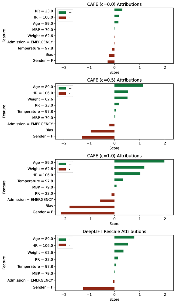
Figure 9: CAFE and DeepLIFT Rescale attribution scores for a correctly classified positive sample from our MIMIC-IV dataset (prediction score 0.51)

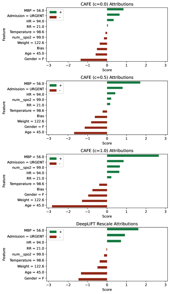
Figure 10: CAFE and DeepLIFT Rescale attribution scores for a correctly classified negative sample from our MIMIC-IV dataset (prediction score 0.23)

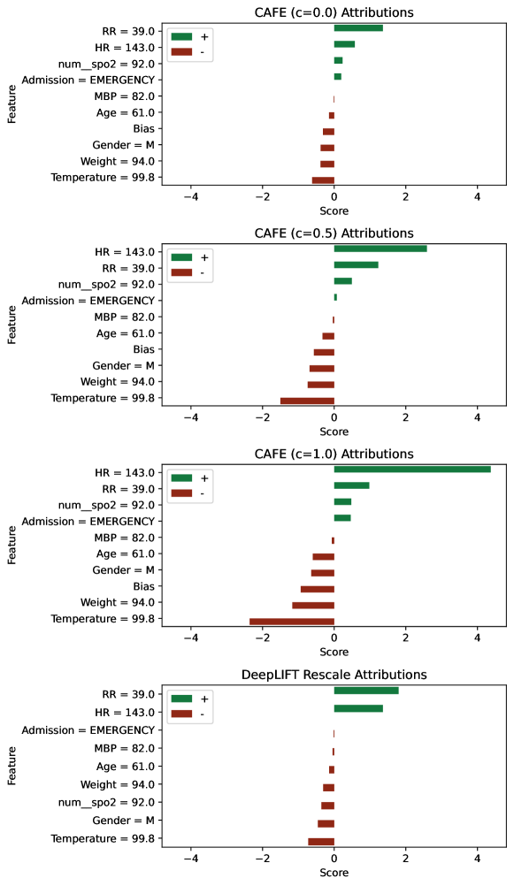
Figure 11: CAFE and DeepLIFT Rescale attribution scores for an incorrectly classified negative sample from our MIMIC-IV dataset (prediction score 0.63)

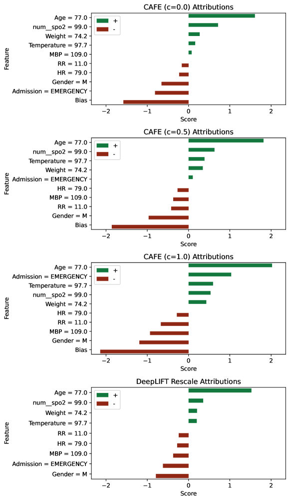
Figure 12: CAFE and DeepLIFT Rescale attribution scores for an incorrectly classified positive sample from our MIMIC-IV dataset (prediction score 0.35)

In the first example (Figure 9) showing attributions for a true positive, we can see that all methods except for CAFE (0.0) considered the high age to be the key feature for predicting a higher likelihood of 30-day mortality, which seems intuitive. It is possible that the age feature partially interfered with the other features or the bias, explaining why it was not well captured by CAFE (0.0). Additionally, we can observe that in comparison to DeepLIFT, CAFE identifies a strong negative effect of the bias. This is to be expected, as the model was trained on a partially imbalanced dataset with a majority of negative samples. Female gender is identified by all methods as a strongly negatively contributing feature, which may be somewhat counterintuitive. Our hypothesis is that the model may be using the gender attribute for a partial representation of its default bias against predicting a positive label, for both of its possible values. This hypothesis also seems to be supported by the attributions scores for the other examples, where the gender attribute always has a relatively strong negative effect on the prediction, regardless of whether it is male or female (though a female gender seems to be associated with stronger negative biases in our examples).

In the second example (Figure 10, we consider the attribution scores for a correctly classified negative sample. We can see that the most strongly contributing features identified by all the considered methods, are a low mean blood pressure and an urgent admission, both reasonable features in the given context. In comparison with other methods, CAFE (0.5) and CAFE (1.0) identify the relatively low age of 45 as a more important feature, which again seems intuitive. All variants of CAFE capture a non-negligible negative effect of the bias, though relatively less important than in the previous example.

The third example (Figure 11) considers an incorrectly classified negative sample. In this case, the relatively high respiratory rate and heart rate are most important for the positive classification. This is reasonable, as high rates for these vital signs typically indicate higher distress and an overall worse clinical state of the patient. Variants of CAFE with higher cancellation sensitivity constant consider the heart rate to be the more important of the two features, while CAFE (0.0) and DeepLIFT state the opposite.

Finally, the fourth example (Figure 12) perhaps most clearly demonstrates the advantage of considering the effect of the bias in the attribution scores. Here, the incorrect negative classification of the model seems to be predominantly caused by the negative bias, which counteracted otherwise strong positively contributing features, such as the high age (77 years). While all variants of CAFE clearly show this, DeepLIFT does not.

Appendix G FAQ

In this section, we provide answers to several questions that may be relevant to practitioners and researchers wishing to use or build upon CAFE in their work.

G.1 What activation functions and model classes are supported by CAFE?

In our experiments, we evaluated CAFE on networks using the ReLU and GELU activations, as we consider these to be one of the most common choices for recent neural architectures. Nevertheless, CAFE does not make any particular assumptions regarding the used activation function, and is thus readily applicable to networks using other common activation functions, such as tanh, sigmoid, swish or softplus. In theory, CAFE may fail to produce reasonable attribution scores for highly irregular activation functions with high numbers of local maxima and minima. However, such functions would likely be unsuitable for use in neural networks, so we do not see this to be a practical limitation.

As implemented and used in our work, CAFE is directly applicable to feedforward model architectures. However, we believe that it would be relatively easy to extend to other kinds of models, such as convolutional neural networks and networks using residual connections. As described in (Wang et al.,, 2019), specialised operations performed by these networks can often be viewed as linear manipulations with sparse matrices or as applications of special activation functions. Similarly, CAFE could also be adapted to transformers using an approach analogical to the one recently proposed for LRP (Ali et al.,, 2022). Further investigation of these extensions poses a promising line of future work.

G.2 What values should I use for the cancellation sensitivity constants?

Typically, the choice of the cancellation sensitivity constants $c^{(n)}$ should be guided by the particular use-case for the produced attribution scores. In cases where simpler and less noisy explanations are desired, it might be preferable to use lower $c^{(n)}$s. However, we would generally advise against using the value of $0$, as we believe that at least a limited ability to surface conflicts is crucial for producing faithful explanations — see the introduction of our paper for the relevant discussion. Meanwhile, in cases in which a greater sensitivity to conflicts is preferred and where more noisy scores are less of a concern, we would recommend the use of larger values of $c^{(n)}$. In the absence of any specific preferences, a value of $c^{(n)}=0.5$ appears to be a sensible default based on our experimental results on real data. Alternately, the value of $c^{(n)}$ could be tuned to maximize the fidelity to the considered model and data. In the case of deeper models with a larger number of layers, we would suggest using lower values of $c^{(n)}$ for lower layers and higher values for later layers, as the conflicts in later layers would typically be more relevant to the model output.

G.3 What value should I use for the reference input?

Similarly to the cancellation sensitivity constant, the appropriate reference input is likely to be context-dependent. For continuous tabular data, vectors of zeroes or mean/median values are common choices. We believe the zero values to be a slightly more principled choice, as it forces the reference model (i.e., the model without biases) to output zero in regression tasks or a uniform distribution in classification tasks. Given this, the completeness property ensures that all changes from this base output are explained by the attribution scores. Additionally, the zero reference is the only option that guarantees that the model does not use any of the reference values in its computations, potentially masking their effect on the prediction during the computation of the attribution scores. Nevertheless, the use of zero reference vectors could also be criticised, as these will often be outside of the data manifold, making the corresponding attributions potentially less grounded in the behaviour of the model on the data distribution. From this point of view, the use of mean or median values may be more appropriate. For categorical data, we believe that a reasonable choice of reference is again zero, although the mode or a domain-specific base category may also be reasonable choices.

G.4 Are there any benefits to using CAFE if I do not care about capturing conflicts between features?

Firstly, we would like to highlight that consideration of conflicts is helpful for producing explanations with a higher fidelity, as evidenced in our experiments. Thus, we believe that using CAFE with non-zero conflict sensitivity constants may produce generally more useful attribution scores, even if surfacing conflicts is not the explicit goal. Nevertheless, even using CAFE (0.0) offers several potential advantages over other methods — in particular, quantifying the effects of the bias, safeguarding against attribution score explosion and distinguishing between positive and negative attribution scores.

G.5 What are the considerations to take when explaining models using CAFE?

Note that the attribution scores computed by CAFE (as well as other attribution methods) are only approximations of the true behaviour of the explained model and may not provide a fully accurate account of the effects of the individual input features. In particular, “reasonably-looking” attribution scores for a particular example are not necessarily a guarantee that the explained model functions correctly or makes correct decisions. Past research has also suggested that cognitive biases of explanation recipients may lead them to incorrect judgements about the behaviour of the model even if the generated scores are accurate (Chu et al.,, 2020; Ghassemi et al.,, 2021). Thus, while feature attribution scores may help uncover and diagnose issues, they cannot exclude their presence and should be used critically in combination with other model evaluation and verification techniques.

Also, while CAFE aims to accurately identify conflicts and safeguard against attribution score explosion, there are still some cases in which its scores may not fully capture feature conflicts or may overestimate the effects of the input features. See the answers to the below questions for details.

G.6 Are there any cases in which CAFE cannot fully capture conflicts between features?

While CAFE aims to surface most of the conflicts between features, there are some cases in which it is unable to do so, even when using the conflict sensitivity constant of $1$. In particular, CAFE may not always capture hypothetical effects of positive or negative features that are masked by the non-monotonicity of the considered activation function. For example, when considering a GELU neuron with the inputs $x_{1}=-2$ and $x_{2}=-5$, CAFE will conclude that both features have no effect on the output, since $\text{GELU}(-7)-\text{GELU}(0)=0$. This ignores the fact that the GELU function decreases and then increases again on the interval, and that the $x_{1}$ input could change the neuron output to $-0.05$ in the absence of $x_{2}$. Effects cancelled in this way could theoretically be captured by considering all activation function extrema within the intervals examined by CAFE. The computed effects could then be added to both positive and negative attribution scores so as to maintain completeness. Nevertheless, we do not believe that doing so would make the attribution scores particularly more insightful. Additionally, having to consider arbitrary activation function extrema would make our method considerably more complicated.

G.7 Are there any cases in which CAFE overestimates the effects of the input features?

Yes, despite the safeguards against the attribution score explosion problem, CAFE can overestimate the possible effects of certain features. For example, consider a model $\mathcal{M}(x)=\text{ReLU}(-\text{ReLU}(1-x))$. It is easy to see that the output of this model will always be zero regardless of the value of $x$, even if the bias is removed. Nevertheless, for an input $x=1$, CAFE (1.0) computes attribution score of $+1$ for $x$ and $-1$ for the bias. This is because the CAFE activation rule can only consider the local behaviour at the individual neurons rather than the global behaviour of the model.

G.8 Are there any relations between CAFE and other feature attribution methods?

Since CAFE (0.0) effectively computes average gradients of the non-linearities (with additional adjustments safeguarding against attribution score explosion), its combined positive and negative scores are equivalent to Gradient $\cdot$ Input, LRP and DeepLIFT when computed with respect to a zero reference input for a network with ReLU activations and no additive biases. This is because the linear attribution flow clipping does not affect CAFE attributions computed for ReLU networks, since the slope of the activation function on its active range is constant.

G.9 The definitions in the paper only describe how to compute the individual elements of the CAFE attribution scores. Is it possible to vectorise these operations?

Yes, computations of the CAFE scores can be easily vectorised and batched with the use of indicator vectors and matrices to switch between the different cases from our definitions. Please see our code for an example of how this can be done — it relatively closely follows the definitions from the main text.

References

- Agarwal et al., (2022) Agarwal, C., Krishna, S., Saxena, E., Pawelczyk, M., Johnson, N., Puri, I., Zitnik, M., and Lakkaraju, H. (2022). OpenXAI: Towards a transparent evaluation of model explanations. Advances in Neural Information Processing Systems, 35:15784–15799.
- Ali et al., (2022) Ali, A., Schnake, T., Eberle, O., Montavon, G., Müller, K.-R., and Wolf, L. (2022). XAI for transformers: Better explanations through conservative propagation. In Chaudhuri, K., Jegelka, S., Song, L., Szepesvari, C., Niu, G., and Sabato, S., editors, Proceedings of the 39th International Conference on Machine Learning, volume 162 of Proceedings of Machine Learning Research, pages 435–451. PMLR.
- Ancona et al., (2018) Ancona, M., Ceolini, E., Öztireli, C., and Gross, M. (2018). Towards better understanding of gradient-based attribution methods for deep neural networks. In 6th International Conference on Learning Representations, ICLR 2018, Vancouver, BC, Canada, April 30 - May 3, 2018, Conference Track Proceedings. OpenReview.net.
- Angwin et al., (2016) Angwin, J., Larson, J., Mattu, S., and Kirchner, L. (2016). Machine Bias.
- Ayoobi et al., (2023) Ayoobi, H., Potyka, N., and Toni, F. (2023). SpArX: Sparse Argumentative Explanations for Neural Networks. In In proceedings of the 26th European Conference on Artificial Intelligence, ECAI 2023, volume 372 of Frontiers in Artificial Intelligence and Applications, pages 149 – 156, Kraków, Poland. IOS Press.
- Bach et al., (2015) Bach, S., Binder, A., Montavon, G., Klauschen, F., Müller, K.-R., and Samek, W. (2015). On pixel-wise explanations for non-linear classifier decisions by layer-wise relevance propagation. PloS one, 10(7):e0130140.
- Balduzzi et al., (2017) Balduzzi, D., Frean, M., Leary, L., Lewis, J., Ma, K. W.-D., and McWilliams, B. (2017). The shattered gradients problem: If resnets are the answer, then what is the question? In International Conference on Machine Learning, pages 342–350. PMLR.
- Chen et al., (2022) Chen, Z., Subhash, V., Havasi, M., Pan, W., and Doshi-Velez, F. (2022). What makes a good explanation?: A harmonized view of properties of explanations. In Workshop on Trustworthy and Socially Responsible Machine Learning, NeurIPS 2022.
- Chu et al., (2020) Chu, E., Roy, D., and Andreas, J. (2020). Are visual explanations useful? a case study in model-in-the-loop prediction. arXiv preprint arXiv:2007.12248.
- Dhurandhar et al., (2018) Dhurandhar, A., Chen, P.-Y., Luss, R., Tu, C.-C., Ting, P., Shanmugam, K., and Das, P. (2018). Explanations based on the missing: Towards contrastive explanations with pertinent negatives. In Proceedings of the 32nd International Conference on Neural Information Processing Systems, NIPS’18, page 590–601, Red Hook, NY, USA. Curran Associates Inc.
- FICO, (2022) FICO (2022). Explainable Machine Learning Challenge.
- Ghassemi et al., (2021) Ghassemi, M., Oakden-Rayner, L., and Beam, A. L. (2021). The false hope of current approaches to explainable artificial intelligence in health care. The Lancet Digital Health, 3(11):e745–e750.
- Guidotti et al., (2018) Guidotti, R., Monreale, A., Ruggieri, S., Turini, F., Giannotti, F., and Pedreschi, D. (2018). A survey of methods for explaining black box models. ACM Comput. Surv., 51(5).
- Hofmann, (1994) Hofmann, H. (1994). Statlog (German Credit Data).
- Johnson et al., (2023) Johnson, A. E. W., Bulgarelli, L., Shen, L., Gayles, A., Shammout, A., Horng, S., Pollard, T. J., Moody, B., Gow, B., wei H. Lehman, L., Celi, L. A., and Mark, R. G. (2023). MIMIC-IV, a freely accessible electronic health record dataset. Scientific Data, 10.
- Kokhlikyan et al., (2020) Kokhlikyan, N., Miglani, V., Martin, M., Wang, E., Alsallakh, B., Reynolds, J., Melnikov, A., Kliushkina, N., Araya, C., Yan, S., and Reblitz-Richardson, O. (2020). Captum: A unified and generic model interpretability library for PyTorch. CoRR, abs/2009.07896.
- Le et al., (2023) Le, P. Q., Nauta, M., Nguyen, V. B., Pathak, S., Schlötterer, J., and Seifert, C. (2023). Benchmarking eXplainable AI - A survey on available toolkits and open challenges. In International Joint Conference on Artificial Intelligence.
- Loshchilov and Hutter, (2019) Loshchilov, I. and Hutter, F. (2019). Decoupled weight decay regularization. In 7th International Conference on Learning Representations, ICLR 2019, New Orleans, LA, USA, May 6-9, 2019. OpenReview.net.
- Lundberg and Lee, (2017) Lundberg, S. M. and Lee, S.-I. (2017). A unified approach to interpreting model predictions. In Proceedings of the 31st International Conference on Neural Information Processing Systems, NIPS’17, page 4768–4777, Red Hook, NY, USA. Curran Associates Inc.
- Meng et al., (2022) Meng, C., Trinh, L., Xu, N., Enouen, J., and Liu, Y. (2022). Interpretability and fairness evaluation of deep learning models on MIMIC-IV dataset. Scientific Reports, 12.
- Montavon et al., (2019) Montavon, G., Binder, A., Lapuschkin, S., Samek, W., and Müller, K.-R. (2019). Layer-wise relevance propagation: an overview. Explainable AI: interpreting, explaining and visualizing deep learning, pages 193–209.
- Nauta et al., (2023) Nauta, M., Trienes, J., Pathak, S., Nguyen, E., Peters, M., Schmitt, Y., Schlötterer, J., van Keulen, M., and Seifert, C. (2023). From anecdotal evidence to quantitative evaluation methods: A systematic review on evaluating explainable AI. ACM Comput. Surv., 55(13s).
- Paszke et al., (2019) Paszke, A., Gross, S., Massa, F., Lerer, A., Bradbury, J., Chanan, G., Killeen, T., Lin, Z., Gimelshein, N., Antiga, L., Desmaison, A., Köpf, A., Yang, E. Z., DeVito, Z., Raison, M., Tejani, A., Chilamkurthy, S., Steiner, B., Fang, L., Bai, J., and Chintala, S. (2019). PyTorch: An imperative style, high-performance deep learning library. In Wallach, H. M., Larochelle, H., Beygelzimer, A., d’Alché-Buc, F., Fox, E. B., and Garnett, R., editors, Advances in Neural Information Processing Systems 32: Annual Conference on Neural Information Processing Systems 2019, NeurIPS 2019, December 8-14, 2019, Vancouver, BC, Canada, pages 8024–8035.
- Pedregosa et al., (2011) Pedregosa, F., Varoquaux, G., Gramfort, A., Michel, V., Thirion, B., Grisel, O., Blondel, M., Prettenhofer, P., Weiss, R., Dubourg, V., Vanderplas, J., Passos, A., Cournapeau, D., Brucher, M., Perrot, M., and Duchesnay, E. (2011). Scikit-learn: Machine learning in python. J. Mach. Learn. Res., 12(null):2825–2830.
- Pezeshkpour et al., (2021) Pezeshkpour, P., Jain, S., Singh, S., and Wallace, B. C. (2021). Combining feature and instance attribution to detect artifacts. CoRR, abs/2107.00323.
- Rahnama, (2023) Rahnama, A. H. A. (2023). The blame problem in evaluating local explanations, and how to tackle it.
- Ribeiro et al., (2016) Ribeiro, M. T., Singh, S., and Guestrin, C. (2016). “Why should I trust you?”: Explaining the predictions of any classifier. Proceedings of the 22nd ACM SIGKDD International Conference on Knowledge Discovery and Data Mining.
- Shapley, (1953) Shapley, L. S. (1953). 17. A Value for n-Person Games, pages 307–318. Princeton University Press, Princeton.
- Shrikumar et al., (2017) Shrikumar, A., Greenside, P., and Kundaje, A. (2017). Learning important features through propagating activation differences. In Precup, D. and Teh, Y. W., editors, Proceedings of the 34th International Conference on Machine Learning, ICML 2017, Sydney, NSW, Australia, 6-11 August 2017, volume 70 of Proceedings of Machine Learning Research, pages 3145–3153. PMLR.
- Shrikumar et al., (2016) Shrikumar, A., Greenside, P., Shcherbina, A., and Kundaje, A. (2016). Not just a black box: Learning important features through propagating activation differences. arXiv preprint arXiv:1605.01713.
- Simonyan et al., (2013) Simonyan, K., Vedaldi, A., and Zisserman, A. (2013). Deep inside convolutional networks: Visualising image classification models and saliency maps. CoRR, abs/1312.6034.
- Smilkov et al., (2017) Smilkov, D., Thorat, N., Kim, B., Viégas, F. B., and Wattenberg, M. (2017). SmoothGrad: Removing noise by adding noise. CoRR, abs/1706.03825.
- Sokol and Flach, (2020) Sokol, K. and Flach, P. (2020). Explainability fact sheets: a framework for systematic assessment of explainable approaches. In Proceedings of the 2020 Conference on Fairness, Accountability, and Transparency, pages 56–67.
- Strumbelj and Kononenko, (2010) Strumbelj, E. and Kononenko, I. (2010). An efficient explanation of individual classifications using game theory. J. Mach. Learn. Res., 11:1–18.
- Sundararajan et al., (2017) Sundararajan, M., Taly, A., and Yan, Q. (2017). Axiomatic attribution for deep networks. In Precup, D. and Teh, Y. W., editors, Proceedings of the 34th International Conference on Machine Learning, ICML 2017, Sydney, NSW, Australia, 6-11 August 2017, volume 70 of Proceedings of Machine Learning Research, pages 3319–3328. PMLR.
- Wang and Nvasconcelos, (2019) Wang, P. and Nvasconcelos, N. (2019). Deliberative explanations: visualizing network insecurities. In Wallach, H., Larochelle, H., Beygelzimer, A., d'Alché-Buc, F., Fox, E., and Garnett, R., editors, Advances in Neural Information Processing Systems, volume 32. Curran Associates, Inc.
- Wang et al., (2019) Wang, S., Zhou, T., and Bilmes, J. (2019). Bias also matters: Bias attribution for deep neural network explanation. In Chaudhuri, K. and Salakhutdinov, R., editors, Proceedings of the 36th International Conference on Machine Learning, volume 97 of Proceedings of Machine Learning Research, pages 6659–6667. PMLR.
- Yeh et al., (2019) Yeh, C., Hsieh, C., Suggala, A. S., Inouye, D. I., and Ravikumar, P. (2019). On the (in)fidelity and sensitivity of explanations. In Wallach, H. M., Larochelle, H., Beygelzimer, A., d’Alché-Buc, F., Fox, E. B., and Garnett, R., editors, Advances in Neural Information Processing Systems 32: Annual Conference on Neural Information Processing Systems 2019, NeurIPS 2019, December 8-14, 2019, Vancouver, BC, Canada, pages 10965–10976.
- Yeh and hui Lien, (2009) Yeh, I.-C. and hui Lien, C. (2009). The comparisons of data mining techniques for the predictive accuracy of probability of default of credit card clients. Expert Systems with Applications, 36(2, Part 1):2473–2480.
- Zhang et al., (2021) Zhang, Y., Tiňo, P., Leonardis, A., and Tang, K. (2021). A survey on neural network interpretability. IEEE Transactions on Emerging Topics in Computational Intelligence, 5(5):726–742.
- Zhou et al., (2021) Zhou, J., Gandomi, A. H., Chen, F., and Holzinger, A. (2021). Evaluating the quality of machine learning explanations: A survey on methods and metrics. Electronics, 10(5).