Emergent topological ordered phase for the Ising-XY Model revealed by cluster-updating Monte-Carlo method

Abstract

The two-component cold atom systems with anisotropic hopping amplitudes can be phenomenologically described by a two-dimensional Ising-XY coupled model with spatial anisotropy. At low temperatures, theoretical predictions [Phys. Rev. A 72, 053604 (2005)] and [arXiv:0706.1609] indicate the existence of a topological ordered phase characterized by Ising and XY disorder but with 2XY ordering. However, due to ergodic difficulties faced by Monte Carlo methods at low temperatures, this topological phase has not been numerically explored. We propose a linear cluster updating Monte Carlo method, which flips spins without rejection in the anisotropy limit but does not change the energy. Using this scheme and conventional Monte Carlo methods, we succeed in revealing the nature of topological phases with half-vortices and domain walls. In the constructed global phase diagram, Ising and XY type transitions are very close to each other and differ significantly from the schematic phase diagram reported earlier. We also propose and explore a wide range of quantities, including magnetism, superfluidity, specific heat, susceptibility, and even percolation susceptibility, and obtain consistent and reliable results. Furthermore, we observe first-order transitions characterized by common intersection points in magnetizations for different system sizes, as opposed to the conventional phase transition where Binder cumulants of various sizes share common intersections. The results are useful to help cold atom experiments explore the half-vortex topological phase.

I Introduction

In the 1970s, the topological phase and phase transitions were proposed and described by the two-dimensional XY model, which has broad applications including the description of superconductivity in 2D films, 2D crystals, 2D magnets, and various other systems [1, 2, 3, 4]. This phenomenon eventually is called the celebrated Berezinskii-Kosterlitz-Thouless (BKT) transition, as referenced in the papers [1, 2]. The BKT transition typically involves the unbinding of vortex-antivortex pairs on a lattice [5].

An integer vortex is defined as a circulation of the gradient of the angle $\theta$ of the standard XY spins, given by $\oint\nabla\theta\cdot d\vec{\ell}=2\pi n$, where $n$ is an integer. However, when $n$ is a fraction, specifically 1/2, a half-integer vortex emerges in certain modified XY models that include terms like $\text{cos}(2\theta_{i}-2\theta_{j})$ [6]. These half-integer vortices are accompanied by strings or domain walls connecting pairs of them. In some cases, with appropriate adjustments to the system’s parameters, the presence of an Ising phase transition is observed, where the spins flip by an angle of 180 degrees, while the long XY spin-wave still persists [6]. Furthermore, other modified terms such as $\text{cos}(q\theta_{i}-q\theta_{j})$, where $q=3,\cdots,8$, induce additional fractional $1/q$-vortex phases in the magnet [7]. These systems exhibit various interesting phases, including the Potts-type transitions  [8] and the newly ordered phases [9, 10].

Some classical lattice spin systems, can be mapped from and used to study the complex quantum many-body systems, which are difficult, even impractical, for efficient quantum numerical methods [11]. The quantum-to-classical mapping here is not a quantum $d$-dimensional mapping to a $d+1$-dimensional square  [12], but rather, it turns quantum operators into classical variables, keeping the spatial dimensions unchanged. Take the Bose-Hubbard model used to describe ultra-cold atoms as the example, the creation (annihilation) operators, $a^{\dagger}(a)$, can be effectively represented in terms of XY spins via the simple mapping $a^{\dagger}\approx e^{-i\theta}$. The interactions between the freedom $\theta_{i}$ on different lattices can be described by the XY model and the generalized version. In 2007, Cenke Xu [13] established a mapping from the two-component Bose-Hubbard model [14] to the double-layer XY model with variables $\theta_{1}$ and $\theta_{2}$ and eventually to the Ising-XY model, featuring spatial anisotropy.

There is a need for large-scale numerical investigations of the Ising-XY model. Firstly, Ref. [13] provides the theoretical analysis and the schematic phase diagram for this model, but there is a lack of published works on related numerical tests to validate these predictions due to some difficulties. Secondly, in the anisotropic limit, the spatially anisotropic Ising-XY model is predicted to exhibit an interesting $B_{1(2)}$ phase, characterized by Ising and XY disorder but 2XY $(2\theta_{1}$ $+2\theta_{2})$ order, where $\theta_{1(2)}$ are the XY spins of the layers, respectively. It would be valuable to explore whether this phase truly exists through numerical simulations and reveal the nature of the $B_{1(2)}$ phase. Thirdly, similar to the fully frustrated XY model [15], the presence of interactions among the Ising variables, excited vortices, and domain walls [16, 17] complicates the understanding of phase transitions between different phases. Numerical studies can shed light on these important elements and provide insights into the behaviors of the Ising-XY model.

This paper addresses the previous questions by employing the Wolff Monte Carlo (MC) method, and our proposed line-shaped cluster-updating MC. These approaches help to overcome non-ergodic issues, at low temperatures and at the limit of high anisotropic parameters. Additionally, to ensure the reliability of the results, parallel tempering (replica exchange MC) is implemented as a cross-check method, as described in Ref. [18]. Extensive numerical simulations reveal the existence and stability of the predicted $B_{1(2)}$ phase, originally suggested by Ref. [13]. Furthermore, a refined global phase diagram is presented. Interestingly, an additional first-order phase transition, not previously mentioned, has also been discovered. This study provides a comprehensive understanding of the Ising-XY model through reliable numerical investigations, offering new insights into the system’s phase diagram and uncovering previously unknown phase transitions.

The outline of this paper is as follows. In Sec. II, the model and the predicted and simulated global phase diagram are shown. In Sec. III, the methods and various quantities are described. The results are shown in Sec. IV. The nature of the $B_{1(2)}$ phase and the phase transitions with other phases are discussed in detail in subsections  IV.1-IV.5. Conclusion and discussion are made in Sec. V.

II Vortex, Model and global phase diagram

II.1 Vortex and anti-vortex

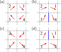
Figure 1: (a) integer vortex, and (b) half-integer vortex and (c) integer anti-vortex, (d) half-integer anti-vortex. The blue line is the domain wall between two spins in a half- integer vortex with an angular difference close to $\pi$.

The integer vortices, half-integer vortices and mathematical descriptions are given here before the specific physical models are presented. In Fig. 1 (a), the integer vortex is shown. Mathematically, it is defined by the four spins around a plaquette $\square{}$. The four spin angles $\theta_{i}$, $i=1,2,3,4$, can be restricted to [$-\pi$, $\pi$] by $\pm 2\pi$. The sum of the differences between adjacent spins is defined as $2\pi n=(\theta_{2}-\theta_{1})+(\theta_{3}-\theta_{2})+(\theta_{4}-\theta_{3})+(\theta_{1}-\theta_{4})$. $2\pi\mathcal{V}$ is naturally equal to 0 if four values in the brackets $()$ are in the range (-$\pi$, $\pi$]. However, whenever any of these values in brackets exceeds the range, there is a possibility of nonzero vorticity by the saw-tooth function, defined by [19]

$$\text{saw}(\theta_{i}-\theta_{j})=\begin{cases}\theta_{i}-\theta_{j}+2\pi,&\theta_{i}-\theta_{j}\leq-\pi,\\ \theta_{i}-\theta_{j},&-\pi<\theta_{i}-\theta_{j}\leq\pi,\\ \theta_{i}-\theta_{j}-2\pi,&\pi<\theta_{i}-\theta_{j}.\end{cases}$$ (1)

Using the configurations in Fig. 1 (a), $\theta_{1,2,3,4}=-\pi/4$, $\pi/4$, $3\pi/4$, $-3\pi/4$, one can get $\Delta\theta_{i,j}=\pi/2$, $\pi/2$, $-3\pi/2$, $\pi/2$. Without using the the saw-tooth function, the sum $\sum\Delta\theta_{i,j}=0$. Using the saw-tooth function, $\sum\Delta\theta_{i,j}=2\pi n,n=1$.

In Fig. 1 (b), the angles are $\theta_{1,2,3,4}=-\pi/8$, $\pi/8$, $3\pi/8$, $-3\pi/8$, and one can get $\Delta\theta_{i,j}=\pi/4$, $\pi/4$, $-3\pi/4$, $\pi/4$. Using the saw function with the modified bounding range $(-\pi/2$ , $\pi/2]$, we can get $\sum\Delta\theta_{i,j}=2\pi n,n=1/2$. In other words, the spin plaquette corresponding to the half-vortex in the configuration $\{\theta_{i}\}$ is also the integer vortex plaquette corresponding to the $\{2\theta_{i}\}$ configuration [20].

II.2 Models

The Bose-Hubbard model, which describes cold atoms with $p_{x}$ and $p_{y}$ orbitals, can be mapped to the double-layer XY model [13]. The Hamiltonian of this model is composed of three terms: $H=H_{up}+H_{dn}+H_{updn}$. $H_{up}$ , $H_{dn}$ , and $H_{updn}$ represent the interaction of spins within the upper layer, within the lower layer, and between the two layers, respectively. These terms are given by :

$$H_{up} =\sum_{i}\left[-J_{a}\cos\left(\nabla_{x}\theta_{i,j,1}\right)-J_{b}\cos\left(\nabla_{y}\theta_{i,j,1}\right)\right],$$ (2)

$$\ H_{dn} =\sum_{i}\left[-J_{b}\cos\left(\nabla_{x}\theta_{i,j,2}\right)-J_{a}\cos\left(\nabla_{y}\theta_{i,j,2}\right)\right],$$ (3)

$$\ H_{updn} =\sum_{i}\left[\gamma\cos\left(2\theta_{i,j,1}-2\theta_{i,j,2}\right)\right].$$ (4)

Here, $J_{a}$, $J_{b}$, and $\gamma$ represent the interaction strengths. It is proposed that the XY spins between the two layers are perpendicular to each other along the vertical direction [13]. To account for this perpendicular alignment, the Ising variable $\sigma$ is introduced, satisfying the relation

$$\theta_{2}=\theta_{1}+\sigma\pi/2.$$ (5)

By substituting this relation into the Hamiltonian and disregarding the constant term $H_{updn}=-\gamma$, the resulting model is the Ising-XY model with spatial anisotropy [13], given by:

$$H =\sum_{\langle i,j\rangle_{x}}-\left(J_{b}+J_{a}\sigma_{i,j}\sigma_{i+\vec{x},j}\right)\cos(\theta_{i,j}-\theta_{i+\vec{x},j})\$$

$$\quad+\sum_{\langle i,j\rangle_{y}}-\left(J_{a}+J_{b}\sigma_{i,j}\sigma_{i,j+\vec{y}}\right)\cos(\theta_{i,j}-\theta_{i,j+\vec{y}}),$$ (6)

where, $\sigma_{i,j}$ represents the Ising spin variables, $\theta_{i,j}$ represents the XY spin variables on the lattice site $(i,j)$, and $\langle i,j\rangle_{x}$ and $\langle i,j\rangle_{y}$ indicate nearest-neighbor interactions in the horizontal ($x$) and vertical ($y$) directions, respectively. In particular, $\theta_{1}$ denotes the spin angle in the bilayer XY model before the mapping, and $\theta$ denotes the spin angle in the Ising-XY model after the mapping Eq. 5.

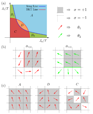
Figure 2: (a) Schematic phase diagram of the model in Eq. 6 and (b) typical configurations $\{\theta_{1}\}$ and $\{\theta_{2}\}$ of the half vortex in the phases $B_{1}$ or $B_{2}$ presented by Ref. [13]. (c) typical configurations of the phase $A$, $D$ and $C$. Red arrows mean the XY spins $\theta_{1}$, gray and white squares represent the Ising spins ($\sigma=1$ and $-1$). The XY spins $\theta_{2}$ can be obtained by the mapping in Eq. 5.

II.3 Phase diagram

Figure 2(a) shows the schematic phase diagram of the model in Eq. 6 at finite temperature [13]. It contains the four phases $A$, $B_{1(2)}$, $C$, and $D$. The phase diagram is symmetric about the $J_{a}=J_{b}$ axis in the plane $J_{a}/T-J_{b}/T$. In order to demonstrate the configurations of each phase, the gray square represents the upward-oriented Ising spin ($\sigma_{i}=1$), while downwards spins are represented by the color white ($\sigma_{i}=-1$). The red arrows indicate the XY spins $\theta_{1}$ in the upper layer. The green arrows indicate the XY spins $\theta_{2}$ in the lower layer.

Figure 2(b) illustrates two typical configurations in the $B_{2}$ phase as illustrated in Refs. [14, 13]. The vertical dashed red line denotes the domain wall of the XY spin $\theta_{1}$, while the XY spin in the other layer, $\theta_{2}$ exhibits domain walls in the horizontal direction through Eq. 5. The main characteristic of the $B_{2}$ phase is the absence of Ising order (sum of Ising variables) due to the presence of numerous domain walls in the actual simulations. Similarly, the long-range XY spin order, as seen in the configurations of $\chi=\theta_{1}+\theta_{2}$, is also expected to be disorder due to the domain walls for the XY spins. However, it is predicted that the $B_{2}$ phase exhibits ordered for the configuration of $2\chi=2\theta_{1}+2\theta_{2}$. To provide a clearer understanding of the above terminology, let’s consider the following example. Suppose there are two spins with opposite orientations on each side of the domain wall, i.e., $\theta_{i,j}-\theta_{i+1,j}\approx\pi$, According to Ref. [13], doubling each angle magnifies the angular difference to $2\pi$, i.e., $2\theta_{i,j}-2\theta_{i+1,j}\approx 2\pi$. Consequently, for spins pointing in opposite directions, doubling their angles results in them becoming identically oriented. The above analysis also applies to the domain wall in the $x$-direction for $\theta_{2}$ (not shown). In summary, the phase $B_{2}$ is predicted to behave in both Ising and XY ($\chi=\theta_{1}+\theta_{2}$) disorder but 2XY ($2\chi$) ordered.

Figure 2 (c) depicts configurations of the phases $A$, $D$, and $C$. The phase $A$ corresponds to an ordered configuration of both Ising and XY spins, the phase $D$ exhibits the Ising order but XY disorder, and the phase $C$ represents disorder in both Ising and XY spins. The order parameters for these four phases are listed in Table. 1.

Table 1: Different phases and their order parameters

phases/orders	$A$	$C$	$D$	$B_{1}$	$B_{2}$
Ising order	✓	✗	✓	✗	✗
XY order ($\chi$)	✓	✗	✗	✗	✗
2XY order ($2\chi$)	✓	✗	✗	✓	✓

Moreover, in the thermodynamic limit, in the region where $M_{x}$ equals 0, $M_{\theta_{1}}$ also tends to zero, just in a different way. This is shown and discussed in the Sec. IV.2.

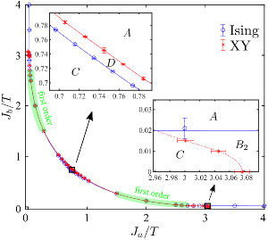
Figure 3: Global phase diagram obtained by the Monte Carlo method. First order phase transitions are found $J_{a}/T=1.5-2.7$. The insets are to make the phase transition boundary visible to the naked eye.

In Fig. 3, we obtain the global phase diagram by the numerical Monte Carlo method. In the plane $J_{a}/T-J_{b}/T$, as shown in Fig. 2, the topology of the phase diagram is consistent with the results predicted by the theory. The phase diagrams still have the $A$, $B_{1}(B_{2})$, $C$, and $D$ phases.

However, as presented by the numerical simulation results, the Ising and XY phase transitions are very close to each other. The change in the sequence of the Ising and XY phase transitions is confirmed. It is difficult to distinguish the two phase transition lines with the naked eye, and for this reason we have drawn enlarged pictures in certain areas, which are placed in the two insets. One inset shows the positions of the $A$, $D$ and $C$ phases. The other inset shows the positions of the $A$, $C$ and $B_{2}$ phases. In the regime $J_{b}/T=0.1,J_{a}/T=1.5-2.7$ marked by green in Fig. 3, first order transitions are found. Other details such as the snapshots of the $B_{1(2)}$ phases are discussed in Sec. IV.

III Methods and Observed quantities

III.1 Methods

In order to construct the global phase diagram, in the anisotropic limit $J_{b}/T\leq 0.2$, we use the combinations of the Metroplis, Wolff, Line-shaped cluster update, and Parallel Tempering MC methods. In the regime $J_{b}/J_{a}\geq 0.2$, we mainly use Wolff and Metroplis algorithms.

(I) Wolff algorithm. For the Ising-XY coupled systems, the Wolff algorithm is used. In the simulation, we first fix the XY spin variables and then update the Ising variables as an effective Ising model with state-dependent interactions as

$$H= \sum_{<i,j>_{x}}-(J_{b}+J_{a}\sigma_{i,j}\sigma_{i+\vec{x},j})J_{XY}^{x}$$ (7)

$$+ \sum_{<i,j>_{y}}-(J_{a}+J_{b}\sigma_{i,j}\sigma_{i,j+\vec{y}})J_{XY}^{y},$$

where $J_{XY}^{x}=cos(\theta_{i,j}-\theta_{i+\vec{x},j})$, $J_{XY}^{y}=\cos(\theta_{i,j}-\theta_{i,j+\vec{y}})$. Then we update the XY spins with fixed Ising variables as with State-dependent interactions,

$$H= \sum_{<i,j>_{x}}-(J_{b}+J_{a}J_{Ising}^{x})\cos(\theta_{i,j}-\theta_{i+\vec{x},j})$$ (8)

$$+ \sum_{<i,j>_{y}}-(J_{a}+J_{b}J_{Ising}^{y})\cos(\theta_{i,j}-\theta_{i,j+\vec{y}}),$$

where $J_{Ising}^{x}=\sigma_{i,j}\sigma_{i+\vec{x},j}$ and $J_{Ising}^{y}=\sigma_{i,j+\vec{y}}$. A MC step performs the updates of the above two Hamiltonians sequentially. This version of Wolff is called cluster-embedding update [21], which has been used simulated Potts-XY model [22].

Figure 4: Schematic diagram of line-shaped cluster update. (a) and (b) update along the $x$-direction with flipping only the Ising spins; (c) and (d) update along the $y$-direction, flipping both the Ising spins and rotating the angle of the XY spin $180^{\circ}$

(II) Line-shaped cluster-update MC. There are difficulties in applying the Wolff or the Metropolis methods alone at low temperatures. The difficulty is the ergodic problem. The $B_{2}$ phase is predicted Ising disordered [13], but such disordered state cannot be reached if the initial state starts from an ordered state with all the same spins. In lower temperatures, and using the metropolis scheme, the states are frozen in the energy local-minimum state and it is difficult to move the spin state across the excited state to global ground state. Traditionally, at lower temperatures, the Wolff cluster is very large, and it can not capture the real information of spin correlations.

The basic idea of the line-shaped cluster MC is as follows. In the parameter limit $J_{b}=0$, one can flip randomly without rejecting the spins within the clusters as the energy does not change. The energies of the configurations in Fig. 4 (a) and Fig. 4 (b) are the same by substituting $J_{b}=0$ into Eq. 7.

Similarly, in the second line of Eq. 8, in the $y$-direction, one rotates the XY spins with angles $\pi$ simultaneously. To fix the energy term in the $x$-direction, one has to flip both the Ising variables simultaneously. Specifically, this can be illustrated by the following equation

$$\begin{split}J_{a}\sigma_{i,j}\sigma_{i+\vec{x},j}\cos(\theta_{i,j}-\theta_{i+\vec{x},j})\equiv\\ J_{a}(-\sigma_{i,j})\sigma_{i+\vec{x},j}\cos([\theta_{i,j}+\pi]-\theta_{i+\vec{x},j}).\end{split}$$ (9)

The advantage of this scheme is that there is no probability of rejection and it can help us to explore the $B_{2}$ phase at $J_{b}=0$ very well.

In the parameter regime $J_{b}\neq 0$ but very close to $0$. One can use the Metropolis method to accept or reject the flip of the spins in the above line-shaped clusters defined as follows:

$$\Delta E_{1} =\sum_{i=1}^{L}\sum_{y}^{\pm 1}2J_{b}\sigma_{i,j}\sigma_{i,j+y}\cos{(\theta_{i,j}-\theta_{i,j+y})}$$

$$\Delta E_{2} =\sum_{j=1}^{L}\sum_{x}^{\pm 1}2J_{b}\cos{(\theta_{i,j}-\theta_{i+x,j})}$$

$$p_{accept} =\left\{\begin{matrix}exp(-\beta\Delta E_{1})&\quad(\text{Fig.~{}\ref{line_cluster_update}(a) $\rightarrow$ (b)})\\ exp(-\beta\Delta E_{2})&\quad(\text{Fig.~{}\ref{line_cluster_update}(c) $\rightarrow$ (d)})\end{matrix}\right.$$ (10)

In the real simulation, we perform $L$ times in each Monte Carlo step to select the directions of the line clusters, which are oriented either horizontally or vertically with a probability of 0.5 and then try to flip the spins within the clusters.

(III) Parallel-Tempering. Parallel-Tempering (PT) is a simulation technique that enhances the efficiency of MC sampling methods [18], especially useful in spin-glass systems [23, 24, 25]. It is particularly effective for systems with complex energy landscapes, where traditional sampling methods may get trapped in local minima. The basic idea behind parallel tempering is to simulate multiple replicas of the system at different temperatures simultaneously. Each replica represents a copy of the system with the same set of spins but at a different temperature. The acceptance probability of an exchange between neighboring replicas satisfies

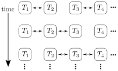
Figure 5: Parallel tempering processes.

$$\begin{split}p&=\min\left(1,\frac{exp\left(-\frac{E_{j}}{T_{i}}-\frac{E_{i}}{T_{j}}\right)}{\exp\left(-\frac{E_{i}}{T_{i}}-\frac{E_{j}}{T_{j}}\right)}\right)\\ &=\min\left(1,e^{\left(E_{i}-E_{j}\right)\left(\frac{1}{T_{i}}-\frac{1}{T_{j}}\right)}\right)\end{split}.$$ (11)

A schematic diagram of replica exchange at different temperatures is given in Fig. 5. The exchange occurs only when executed between neighboring temperatures.

In the actual simulation, we set the temperature range to cover both sides of the phase transition. This approach allows the low-temperature system to feel the influence of the high-temperature system and ensures that the system explores the entire energy landscape, including the local energy minimum. In the case of $J_{b}=0$, the temperature range $(0,1)$ is divided into $250$ equally spaced copies, and $500,000$ steps of relaxation are performed for all the temperature replicas in turn, with one MC step as performing one combination of Wolff, Metropolis, line-shaped cluster update. After performing the above relaxation process, another $2.5$ million updates are performed and the temperature replicas are randomly selected to try to exchange after every $5$ Monte Carlo steps.

III.2 Algorithmic verification

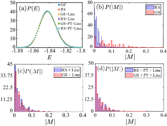
Figure 6: Distribution of energy $P(E)$ and magnetization $P(M)$ for different methods and different initial configurations. (a) The same $P(E)$ by three methods with two different initial configurations. (b) $P(M)$ by the Wolff method, (c) $P(M)$ by the Wolff+line method, and (d) $P(M)$ by the Metropolis+Wolff+Line+PT method.

In Fig. 6, we compare the effects of the combination of different methods at low temperatures and in the anisotropic limit. In total, there are 3 methods, one is a pure Wolff+Metropolis method, the second is a Wolff+Metropolis+Line method, and the third is a Wolff+Metropolis+Line+PT method, and 5 million samples for the histogram. As a generic scheme for updating, the Wolff+Metropolis method is not labeled. The three methods utilize different initial configurations, random or all the same, i.e., marked by “RS” and “GS”. With parameters $L=24$, $J_{b}=0$, $T=0.3$, for the distribution of the energy and Ising magnetization are measured.

In Fig. 6 (a), the distribution of energy $P(E)$ is the same for all methods with different initial states. In Fig. 6 (b), for the first method (Wolff+Metropolis), $P(M)$ is not consistent for different initial states. As seen in Fig. 6 (c), based on the already existing Wolff + Metropolis method, the line- shaped cluster-update MC algorithm allows a high degree of overlap between $P(M)$ obtained for the two initial states. A slight deviation could be due to the fluctuation of the distribution, and another possible reason is that the Line-shaped cluster scheme doesn’t exactly help with the states ergodic. Finally, in Fig. 6 (d), the Wolff+line+PT method helps $P(M)$ overlap in a way that the naked eye can’t see the difference.

III.3 Observed quantities

(i@) Both the BKT and Ising phase transitions can be described by the magnetic order parameters, defined by the Ising magnetization and the XY magnetization defined as,

$$M_{\text{I}}=\frac{1}{N}\expectationvalue{\absolutevalue{\sum_{i}\sigma_{i}}},$$ (12)

$$M_{\theta}=\frac{1}{N}\left\langle\sqrt{\left(\sum_{j}\sin\theta_{j}\right)^{2}+\left(\sum_{j}\cos\theta_{j}\right)^{2}}\right\rangle,$$ (13)

where $\sigma=\pm 1$ represents the Ising spin, $\theta\in[0,2\pi]$ represents the XY spin, and $N$ represents the total number of lattice sites. $M_{\theta}$ is used to define the BKT phase transition with respect to $\theta$, similarly, $M_{\chi}$ and $M_{2\chi}$ can be defined as magnetization order parameters by the variables $\chi$ and $2\chi$. Note that $\theta_{2}=\theta_{1}+\sigma\frac{\pi}{2}$, and $\chi=\theta_{1}+\theta_{2}$.

(ii@) The binder cumulants [26, 27] of the Ising and XY variables are defined as,

$$U_{2}=\frac{n+2}{2}\left(1-\frac{n}{n+2}R_{2}\right),$$ (14)

where $n=1$ for the Ising magnetization, $n=2$ for the XY model, and $R_{2}$ is Binder ratio [28, 29], in the ordered phase, $U_{2}\xrightarrow{}1$.

$$R_{2}=\expectationvalue{M^{4}}/\expectationvalue{M^{2}}^{2}.$$ (15)

(iii@) Specific heat and susceptibilities. We introduce corresponding susceptibilities for all order parameters ($M_{I},M_{\theta},M_{\chi},M_{2\chi}$),

$$\chi_{s}=\frac{1}{k_{B}T}(\expectationvalue{M^{2}}-\expectationvalue{M}^{2}),$$ (16)

and the specific heat $C_{V}$,

$$C_{v}=\frac{1}{k_{B}T^{2}}(\expectationvalue{H^{2}}-\expectationvalue{H}^{2}).$$ (17)

(iv@) The spin stiffness $\rho_{s}$ is defined as follows [27]:

$$\mathcal{\rho}_{s}=\frac{1}{Nd}[\langle H\rangle-\beta(\langle I^{2}_{x}\rangle+\langle I^{2}_{y}\rangle)],$$ (18)

where $\beta$ is inverse of temperature, $N$ is the total number of spins, $d$ is the dimension, and $I_{x},I_{y}$ defined as

$$I_{x}= \sum_{<i,j>_{x}}(J_{b}+J_{a}\sigma_{i,j}\sigma_{i+\vec{x},j})\sin(\theta_{i,j}-\theta_{i+\vec{x},j}),$$ (19)

$$I_{y}= \sum_{<i,j>_{y}}(J_{a}+J_{b}\sigma_{i,j}\sigma_{i,j+\vec{y}})\sin(\theta_{i,j}-\theta_{i,j+\vec{y}}).$$ (20)

(v@) The bond’s order in $x$- and $y$-directions

$$Bond_{x}=\sum_{<i,j>_{x}}\sigma_{i}\sigma_{j}, Bond_{y}=\sum_{<i,j>_{y}}\sigma_{i}\sigma_{j},$$ (21)

where are useful to characterize the melting of Ising domain walls.

(vi@) The percolation susceptibility [30] $S_{2}$ is defined as

$$S_{2}=L^{-2}\expectationvalue{\sum_{i=1}^{N_{c}-1}n_{i}^{2}},$$ (22)

where one removes the cluster containing the highest number of sites during the summing.

IV Results

In this section, we give numerical results in detail. We first scan the phase diagram along the $J_{a}=J_{b}$ diagonal cut in Sec. IV.1, then we scan the regimes $J_{b}\ll J_{b}$ in Sec. IV.2. The signature of $M_{\theta}$ is also analyzed carefully in Sec. IV.3. The regimes of first order transition is confirmed in range about $J_{a}/T\in(1.5,2.7)$ in Sec. IV.4. At $J_{a}/T=3.5$, the phase transition and Ising type universality between $A-B_{2}$ phase are discussed in Sec. IV.5.

IV.1 Phase transitions between the phases $A-D-C$ along $J_{b}=J_{a}$

In this section, we calculate the Ising phase transition and the XY phase transition at isotropic parameters $J_{b}=J_{a}$ and verify that the XY phase transition occurs earlier than the Ising phase transition from low to high temperature. It is understandable that if Ising emerges as a domain wall, the interaction $(1+\sigma_{i}\sigma_{j})=0$, so the algebraic order of the XY spin can only exist before the Ising phase transition or the phase transitions of XY and Ising occur at the same time. In addition, in the coupled system, we also confirm the universalities by data collapse method on the data with different lattices.

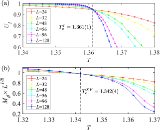
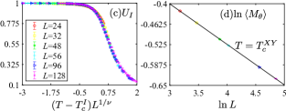
Figure 7: The results along the cut $J_{a}=J_{b}$. (a) the crossing points of $U_{I}$ occur at $T_{Ising}\approx 1.361(1)$, (b) the crossing points of $M_{\theta}L^{\frac{1}{8}}$ occur at $T_{xy}\approx 1.342(4)$. (c) Data collapse of $U_{I}$ (d) $\ln M_{I}$ .vs. $\ln L.$

In Fig. 7 (a), along the diagonal cut $J_{a}=J_{b}$ in the phase diagram, we scan the temperature in the range $T\in[1.34,1.38]$ with lattice sizes $L=24,32,48,56,96,128$. With the increase in temperature, the Ising binder cumulative $U_{I}$ overlap at $T_{c}^{I}\approx 1.361(1)$ for different lattices. At critical regimes,the cumulative moments of the magnetization satisfy the following scaling relationship as [26, 31],

$$\langle M^{k}\rangle_{L}=L^{-k\beta/\nu}\mathcal{F}(\frac{T-T_{C}}{T_{C}}L^{1/\nu}),$$ (23)

where $\mathcal{F}$ is a scaling function. When $T=T_{C}$, the ratio $R_{2}=\langle M^{4}\rangle_{L}/\langle M^{2}\rangle_{L}^{2}$ is independent of $L$, and therefore the data $U_{I}$ for different sizes cross at the critical point.

In Fig. 7 (b), $M_{\theta}L^{1/8}$ vs $T$ is plotted. The data from different sizes also cross at $T=T_{C}$ very well. The reason is as follows. Firstly, the correlation length is proportional to system size as

$$\xi(T)\sim L\sim\lvert\frac{T-T_{C}}{T_{C}}\rvert^{-\nu},$$ (24)

and then

$$M_{\theta}\sim\lvert\frac{T-T_{C}}{T_{C}}\rvert^{\beta}\sim L^{-\beta/\nu}.$$ (25)

Using the critical exponents $\beta=1/8$ and $\nu=1$, the data of $M_{\theta}L^{1/8}$ cross at the same point for different sizes. $M_{\theta}L^{1/8}$ is a very good order parameter to locate the BKT phase transition point $T_{c}^{XY}\approx 1.342(4)$.

To further confirm the Ising transition, we also re-scale $T$ as $(T-T_{C})L^{1/\nu}$, and the data overlap very well as shown in Fig. 7 (c). For the XY transition, leting $k=1$ in Eq. 23, one can get $\langle M_{\theta}\rangle_{L}\propto L^{-1/8}$. Using the log-log plot, the slope is -1/8 as shown in Fig. 7 (d).

By comparison, it can be seen that the XY phase transition $T_{c}^{XY}\approx 1.342(4)$ occurs before the Ising phase transition $T_{c}^{I}\approx 1.361(1)$ as the temperature increases. In the $J_{a}=J_{b}$ limit, the model is approx to the so-called fully-XY model [15, 32], and by re-normalization group [33]. Early on, it was mistakenly thought to be undergoing a single phase transition, due to the fact that there was only one specific heat peak [34, 35]. Finally, this region has been shown to undergo two phase transitions at higher computational accuracy [36] by various methods.

IV.2 Snapshots, and phase transition between the phases $B_{2}-C$ with $J_{b}\ll J_{a}$

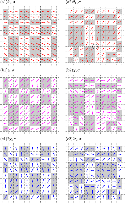
Figure 8: Snapshots Series $\{\theta_{1}$, $\sigma$, $\chi$, $2\chi\}$. Left column: $J_{a}=1$, $J_{b}=0$, $T=0.1$ in the $B_{2}$ phase. Right column: $J_{a}=1$, $J_{b}=0$, $T=0.375$ near the transition point. The Arrows indicate the XY spins, and the shaded squares indicate the Ising spins $\sigma_{i}=1$, and the white squares indicate $\sigma_{i}=-1$. (a) The snapshots of $\{\theta_{1}\}$ and $\{\sigma\}$. The domain walls of $\theta_{1}$ (red) form straight lines aligned in the $y$-direction while the Ising domain walls are represented as closed rectangles. (b) The snapshots of ${\chi=\theta_{1}+\theta_{2}}$ clearly reveal the disorder in $\chi$ with the magnetization $M_{\chi}\approx 0.009$ (left) and $M_{\chi}\approx 0.006$ (right). (c) The snapshot of $\{2\chi\}$ demonstrates the ordered phase, with $M_{2\chi}\approx 0.86$ (left) and $M_{2\chi}\approx 0.367$ (right, near the critical point).

Fig. 8 plots a typical snapshot in the $B_{2}$ phase ($J_{b}/J_{a}=0$), showing the configurations of $\theta_{1}$, $\sigma$, $\chi$ and $2\chi$. The gray squares indicate $\sigma=1$, and the white squares indicate $\sigma=-1$, and the arrows indicating XY spins.

We observe only domain walls inside the $B_{2}$ phase and the half-integer vortex is observed near the transition point between the $B_{2}$ and $C$ phases. Fig. 8 (a), $\theta_{1}$ (red), and $\sigma_{i}$ are shown. $\theta_{2}$ is not shown for clarity purposes, but it can be obtained by Eq. 5. Along different directions of the domain wall, the angle $\theta_{1}$ occurs a $\pi$-flip along the $\mathbb{Z}_{2}$ domain wall in the $y$-direction, while there is no domain wall along the $x$-direction. Conversely, $\theta_{2}$ has a $\pi$-flip along the domain wall in the $x$-direction, while there is no in the $y$ direction (not shown).

Fig. 8 (b) shows the configuration of $\chi=\theta_{1}+\theta_{2}$. It can be seen that the $\chi$ angle inside each shaded block is opposite to the surrounding neighboring spins. There are domain walls in both the $x$ and $y$ directions. Therefore, $M_{\chi}=M_{\theta_{1}+\theta_{2}}\approx 0$ is disordered. Although the actual value in the figure is finite at $M_{\chi}\approx 0.009$, it is found to be zero in the subsequent finite size scaling. Fig. 8 (c) shows the configuration of $2\chi=2\theta_{1}+2\theta_{2}$. For $2\chi$, the domain wall hardly appears anymore, and all the spins point approximately the same way, i.e., $2\chi$ is ordered. In the configuration, the actual value is $M_{2\chi}\approx 0.86$.

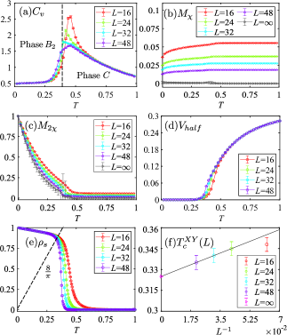
Figure 9: The quantities for the XY variables at $J_{a}=1,J_{b}=0$, and $T_{c}\approx 0.335$. (a) $C_{V}$; (b) the bond orders $Bonds_{x,y}$; (c) $M_{2\chi}$; (d) the density of half-integer vortex (e) the spin stiffness $\rho_{s}$ (f)Extrapolation to obtain the phase-transition point.

Thus, the existence of the $B_{2}$ phase is confirmed and the problem becomes how to determine the phase transition point. Figure 9(a) shows the specific heat $C_{V}$ in the range $T/J_{a}\in[0,1]$ while $J_{b}=0$. Using data for sizes $L=16-48$ it has been shown that, the non-divergent behavior of the specific heat peaks indicates the presence of the BKT phase transition.

As predicted, in both the $B_{2}$ and $C$ phases, $\chi$ is disordered ($M_{\chi}=0,L\rightarrow\infty$) as shown in Fig. 9(b). However, obtaining such data in agreement with expectations is quite challenging. First, the phase transition point corresponds to a very low temperature, around $T_{c}\approx 0.34$. Traditional cluster methods such as the Wolff algorithm are inefficient in this mixed system. As introduced in Sec. III III.1, a combination of various methods including the Metroplis, Wolff, line-shaped cluster and PT methods, is used to obtain results consistent with expectations.

In order to obtain the phase transition point, we analyze the signal of $2\chi$. The first quantity of interest is $M_{2\chi}$ as shown in Fig. 9 (c). In the low-temperature phase with $T<T_{c}$, $M_{2\chi}>0$ and continuously changes smoothly to 0. This suggests that when we magnify the angle by a factor of two, the $2\chi$ ordered state is found from the $\chi$ disordered configuration and remains stable in the thermodynamic limit. Additionally, we assess the density of half-integer vortices, as shown in Fig. 9 (d). In the low-temperature phase, the density of half-integer vortices is zero. In contrast, in the high-temperature phase, numerous half-vortices become excited, resulting in a non-zero density. It’s worth noting that we also measure the integer vortex density, which exhibits non-zero values in both phase $B_{2}$ and phase $C$. However, these results are not presented in this figure.

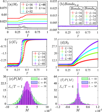
Figure 10: The quantities for the Ising variables ($J_{a}=1,J_{b}=0$). (a) $M_{I}$; (b) the bonds order $Bonds_{x,y}$; (c) $U_{I}$; and (d) the percolation susceptibility $S_{2}$. (e) Distribution of $M_{I}$ in the $C$ phase; (f) the distribution of $M_{I}$ in the $B_{2}$ phase.

In addition, inspired by the formula for the superfluid density of isotropic systems given in the literature [27], we derive an expression for the spin stiffness in the anisotropic case as shown from Eq. 18 to Eq. 20. Within the BKT theory, spin stiffness exhibit a universal jump at $T_{c}$ [37],

$$\rho_{s}=\frac{2}{\nu^{2}\pi}T_{c},~{}~{}\nu=1/2.$$ (26)

The line $8T/\pi$, the spin stiffness data $\rho_{s}$ for various sizes in Fig. 9(e) intersect at the location of the jump $T_{c}\approx 0.325(5)$ and the fitting $T_{c}^{XY}(L)$ vs $L^{-1}$ are shown in in Fig. 9(f).

Next, the phase transition is analyzed from the perspective of the Ising variables. Due to the numerous domain walls in both the $B_{2}$ and $C$ phases, the Ising variables are disordered. Clearly, in Figs. 10(a) and (b), $M_{I}$ is zero as $L\rightarrow\infty$. The average bonds in both directions, described in Eq. 21, are also zeros. However, we see the phase transition signal in terms of the Binder ratio $U_{I}$ corresponding to the Ising variable as well as the percolation susceptibility $S_{2}$ in Figs. 10(c) and (d). In the $C$ phase, the shape of $P(M)$ should be Gaussian as shown in Fig. 10(e). Due to the relations

$$\int_{-\infty}^{\infty}M^{2}\frac{1}{\sqrt{2\pi}}e^{-\frac{M^{2}}{2}}dM=1$$ (27)

and

$$\int_{-\infty}^{\infty}M^{4}\frac{1}{\sqrt{2\pi}}e^{-\frac{M^{2}}{2}}dM=3,$$ (28)

we can get $U_{I}=\frac{3}{2}\left(1-\frac{1}{3}\expectationvalue{M^{4}}/\expectationvalue{M^{2}}^{2}\right)\rightarrow 0$ [26]. In the $B_{2}$ phase, characterized by the quasi-exponential distribution $P(M)=\lambda e^{-\lambda|M|}$ as shown in Fig. 10 (f), we can get $U_{I}<0$. The change in $U_{I}$ from 0 to less than zero reflects the phenomenon of phase transition. Usually, a negative peak of $U_{I}$ represents a first-order phase transition [26]. A negative $U_{I}$, without a negative peak, is not indicative of a first-order phase transition.

IV.3 Signatures of $M_{\theta}$

In this subsection, we list the behaviours of physical quantity $M_{\theta}$, in different phases, as shown in Fig. 11. Because the variables for our numerical simulation are XY spins on one layer $\theta$ and Ising variable $\sigma_{i}$, one might ask whether or not the magnetisation intensity $M_{\theta}$ is 0, except that $M_{\chi}$ is non-zero in phase $B_{2}$.

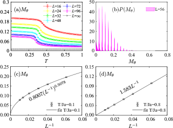
Figure 11: (a) $M_{\theta}$ vs $T$; (b) is the probability distributions of $M_{\theta}$ for sizes $L=56$ when $T/J_{a}=0.1$; (c) and (d) are $M_{\theta}$ vs $L^{-1}$ at different temperatures.

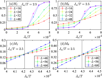
Figure 12: $M_{I}$ and $M_{\theta}$ vs $J_{a}/T$. The intersection positions are close to 0.042 and 0.043, respectively, indicating that the two phase transitions are not at the same location.

In Fig. 11 (a), $M_{\theta}$ vs $T$ is plotted. In the thermodynamic limit, it is not difficult to understand that $M_{\theta}$ is zero in the disordered C phase. But in the $B_{2}$ phase, in addition to the $\chi$-disordered phase characterized by $M_{\chi}=0$, $M_{\theta}$ can also characterize that disordered phase, e.g. $M_{\theta}=0$.

Next, we analyze $M_{\theta}$ through the probability distribution $P(M_{\theta})$ as shown in Fig. 11 (b) at $J_{b}/T=0$. The distribution of $M_{\theta}$ has many discrete peaks. The horizontal coordinates corresponding to these peaks can actually be calculated manually. As shown by the red arrows in the snapshot in Fig. 8 (a), these arrows are almost identical in the vertical direction, i.e. the stripe pattern. Therefore, we simply pick one of the rows of spins to analyze.

The first peak corresponds to a horizontal coordinate of 0, which represents the configuration of the system where there are $L/2$ up spins and $L/2$ down spins. In this case, the probability $P(M_{\theta}=0)$ is proportional to the coefficient $C_{L}^{L/2}$. For the second peak, there are there are $L/2+1$ up spins and $L/2-1$ down spins. Taking $L=56$ for example, the location is $(29-27)/56$ and its probability proportional to $2C_{L}^{L/2-1}$. Thus the ratio of the areas of the two peaks is $C_{L}^{L/2}:2C_{L}^{L/2-1}=0.5208$, which coincides with the results of the MC simulation. We also examine the results at other sizes and other peaks and the conclusions remain the same.

In both the $B_{2}$ and $C$ phases, as the system size approaches infinity in the thermodynamic limit, $M_{\theta}$ converges to 0, but it varies with size in different ways. In Fig. 11 (c), the plot shows $M_{\theta}$ vs. $L^{-1}$ at $T/J_{a}=0.1$ in the $B_{2}$ phase. The data is well fitted with the function $0.8007L^{-0.5078}$. In Fig. 11 (d), in the $C$ phase, the plot of $M_{\theta}$ vs. $L^{-1}$ is well fitted with the function $1.583L^{-1}$ and it decays faster.

In short, the phase $B_{2}$ and phase C, although both are $\theta$ disordered phases, have distinctly different patterns. In the $B_{2}$ phase, the pattern for $\theta$ (red arrows) appears striped, showing disorder only in the $x$ direction, and there are only 2 possibilities for spin direction in the configuration. But in the $C$ phase, the spin is completely disordered, lacking any noticeable pattern.

Table 2: List of parameters and dimensions corresponding to the double-peaked distribution in Fig. 13.

$Ja/T$	$L$	$J_{b}/T(P(E))$	$J_{b}/T(P(M_{I}))$	$J_{b}/T(P(M_{\theta}))$
1.5	48	0.2600	0.2585	0.2580
1.5	72	0.2620	0.2610	0.2606
1.7687	48	0.1761	0.1761	0.1761
1.7687	72	0.1766	0.1766	0.1766
2.0	48	0.1188	0.1188	0.1184
2.0	72	0.1194	0.1194	0.1192
2.7	48	0.0360	0.0440	0.0370
2.7	72	0.0340	0.0360	0.0320

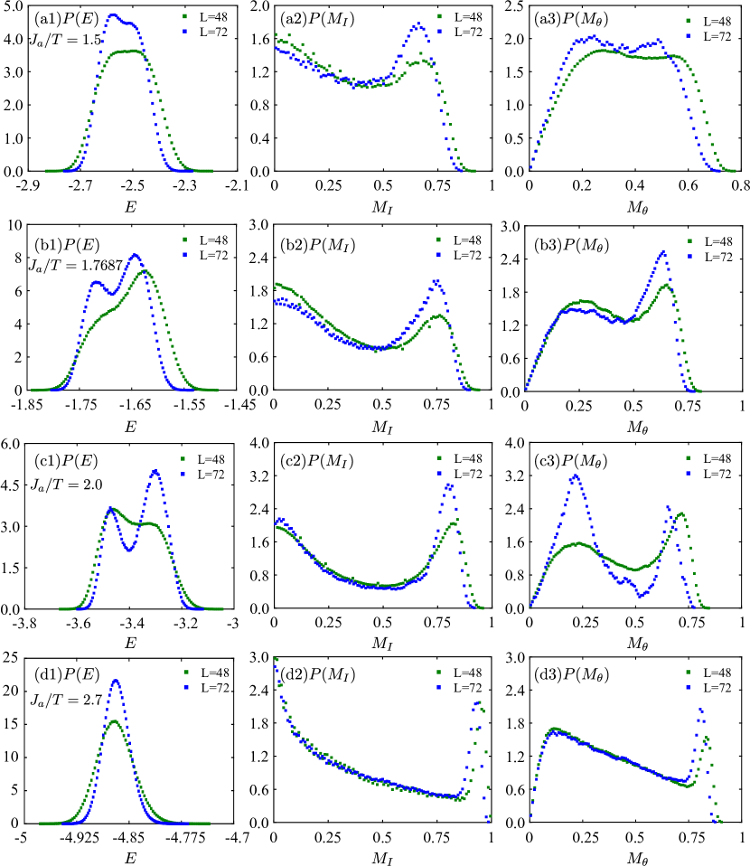
Figure 13: The probability distribution (normalized) of physical quantities near the critical point obtained by fixing the parameter $J_{a}/T$ and scanning $J_{b}/T$. This two-peaked distribution characterizes the first-order phase transition. Details of the parameters are shown in Table. 2.

IV.4 First order transitions along $J_{a}/T=1.5-2.7$

In the global phase diagram in Fig. 3, the regimes marked in green represent first-order phase transitions. Two questions need to be addressed. The first question is whether the Ising first-order phase transition and the XY first-order phase transition occur with the same parameter? Second, what is the signal for the first-order phase transition?

In the results shown in Fig. 12, it is observed that in the region of the first-order phase transition, the phase transitions for the Ising and XY variables still do not occur simultaneously. Fixing $J_{a}/T=2.5$, $M_{I}$ and $M_{\theta}$ versus $J_{b}/T$ are plotted in the range $0-0.08$ and the zoomed range $0.04-0.045$. Apparently, the intersection of $M_{I}$ lines of different sizes is close to 0.042 while the intersection of $M_{\theta}$ lines of different sizes is close to 0.043. Therefore, the two transitions do not occur simultaneously. In this parameter interval, the theoretical predictions [13] of the phase diagram structure and the numerical experiments are in agreement.

In response to the second question, when testing the Binder ratio $U_{I}$ for different sizes, no intersection point is found, but a negative peak is observed [26] (although not shown). In Figure 12, it is intriguing to observe that the magnetization curves, represented by $M_{I}$ and $M_{\theta}$, for different system sizes intersect at the point of phase transition. This intersection is attributed to the symmetry breaking of continuous variables [38]. Further more, the distributions $P(E)$, $P(M_{I})$, $P(M_{\theta})$ are plotted to check whether or not double peaks emerge. At the beginning of the green line, with parameter $J_{a}/T=1.5$, the signatures of the double peaks are weak or even absent, indicating a phenomenon known as pseudo first-order phase transition [39]. As the system size increases, the two peaks in the energy distribution approach each other, as illustrated in Figure 13 (a).

In the regime $J_{b}/T=0.1$, $J_{a}/T=2$ and $J_{a}/T=1.7867$ in Fig. 3, the signature of the first-order transition is the most obvious. The evidence is that the double peaks emerge for the distributions $P(M_{I})$, $P(M_{\theta})$ and $P(E)$ with $L=48,72$ as shown in Figs. 13 (b) and (c). In the end of the green line $J_{a}/T=2.7$, the double peaks of energy disappear. Although both $P(M_{I})$ and $P(M_{\theta})$ exhibit bimodal distributions, which indicates energy degeneracy in the system or coexistence of two phases in the system, it is still not possible to determine whether a first-order phase transition occurs at this point.

It is worth noting that the double peaks observed in $M_{I}$ and $M_{\theta}$ do not occur at the same parameter values $J_{a}/T$ and $J_{b}/T$. There is a deviation between the parameters corresponding to $M_{I}$ and $M_{\theta}$ for different system sizes. Specific values of the parameters are listed in the Table. 2. The parameter difference for $M_{I}$ and $M_{\theta}$, obtained from the same lattice size, indicates that the two phase transitions, do not occur simultaneously.

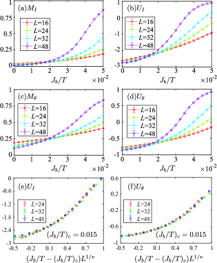
Figure 14: $J_{a}/T=3.5$, (a)$M_{I}$ vs $J_{b}/T$; (b)$U_{I}$ vs $J_{b}/T$; (c)$M_{\theta}$ vs $J_{b}/T$; (d)$U_{\theta}$ vs $J_{b}/T$.

IV.5 $J_{a}/T$=3.5, transitions between the $A$ and $B_{2}$ phases

In Fig. 14, we explore the phase transition between the A-$B_{2}$ phase. By fixing $J_{a}/T=3.5$ and scanning $J_{b}/T$, at this point, we observe that both $M_{I}$ and $M_{\theta}$ for different sizes exhibit common intersections, as reported in Ref. [38] recently.

The Binder ratios $U_{I}$ and $U_{\theta}$ exhibit similar behavior during the phase transition. By performing a data collapse analysis for these two quantities, we plot $U_{I}$ and $U_{\theta}$ as functions of $(T-T_{c})L^{1/\nu}$, for different system sizes. Remarkably, the data points for various sizes overlap with each other. This observation indicates that the critical exponent of the phase transition follows the Ising universal class with $\nu=1$.

V Conclusion

In this paper, we perform large-scale simulations to numerically validate the theoretical results predicted in 2007 [13]. We investigate the spatially anisotropic Ising-XY models using the method of Wolff cluster-updated Monte Carlo (MC) and develop the line-shaped cluster-update MC method to ensure the reliability of our simulation results.

The main findings include exploring clearly the nature of the $B_{2}$ phase and constructing the global phase-diagram. In the anisotropic limit, the $B_{2}$ phase is confirmed Ising and XY disorder, but 2XY order, i.e., $M_{I}=0$, $M_{\chi}=0$ and $M_{2\chi}\neq 0$. Numerical simulations reveal domain walls as dominant within the $B_{2}$ phase, while the half-integer vortices occur at the phase boundary between the $B_{2}$-$C$ phases. The phase transition between $B_{2}$ and $C$ phases is confirmed to be the BKT type with half-integer vortex, as the superfluid density is found to scale as $\rho_{s}=\frac{2}{\nu^{2}\pi}T_{c}$, with the exponent being equal to $\nu=1/2.$

In addition, more details beyond the theory are revealed. In the isotropic limit, the critical points of the Ising are XY phase transitions have been identified at $T_{c}^{I}=1.361(1)$ and $T_{c}^{XY}=1.342(2)$, respectively. In the anisotropic limit, the snapshots within the $B_{2}$ phase are checked very carefully. The XY spins exhibit a quasi-one-dimensional pattern. The magnetization $M_{\theta}(L)$ in the in the $B_{2}$ phase follows a scaling behavior of $M_{\theta}(L)=0.8007L^{-0.5078}$, while in the high temperature disorder $C$ phase, it follows a different scaling behavior of $M_{\theta}(L)=1.583L^{-1}$.

In the parameter regions that deviate from the isotropic and anisotropic limits, both phase transitions become first-order phase transitions. Interestingly, $M_{I}$ and $M_{\theta}$ of different sizes intersect at a point due to continuous symmetry breaking [38]. These phenomena are determined by the double-peaked distribution of the energy. As to whether there is new critical exponents [35], further large-scale calculations are needed in the future.

Indeed, the physics of the Ising-XY model with spatial anisotropy extends beyond two-dimensional lattice systems and can also be observed in three-dimensional systems. This insight was highlighted in the study [13].

The physics of the Ising-XY model for spatial anisotropy is not limited to the two-dimensional lattice system, and can also be observed in the three-dimensional system. This insight was highlighted in the study [13]. Furthermore, one can study the Bose-Hubbard model with $p_{x}$ and $p_{y}$ orbitals directly  [13]. These studies are left for future exploration.

Our result can help understand the half-integer vortex in possible cold-atom theory [14], but it can be realized by cold-atom experiment [40]. Furthermore, our approach offers a case study that demonstrates the mapping of diverse novel states in complex quantum systems to classical systems, enabling large-scale simulations [13].

References

- Berezinsky [1972] V. L. Berezinsky, Sov. Phys. JETP 34, 610 (1972).
- Kosterlitz and Thouless [1972] J. M. Kosterlitz and D. J. Thouless, Journal of Physics C: Solid State Physics 5, L124 (1972).
- Chen et al. [2020] K. Chen, D. J. Srolovitz, and J. Han, Proceedings of the National Academy of Sciences 117, 33077 (2020), https://www.pnas.org/doi/pdf/10.1073/pnas.2017390117 .
- Fraggedakis et al. [2023] D. Fraggedakis, M. R. Hasyim, and K. K. Mandadapu, Proceedings of the National Academy of Sciences 120, e2209144120 (2023), https://www.pnas.org/doi/pdf/10.1073/pnas.2209144120 .
- Kosterlitz [2017] J. M. Kosterlitz, Rev. Mod. Phys. 89, 040501 (2017).
- Lee and Grinstein [1985] D. H. Lee and G. Grinstein, Phys. Rev. Lett. 55, 541 (1985).
- Canova et al. [2014] G. A. Canova, Y. Levin, and J. J. Arenzon, Phys. Rev. E 89, 012126 (2014).
- Drouin-Touchette et al. [2022] V. Drouin-Touchette, P. P. Orth, P. Coleman, P. Chandra, and T. C. Lubensky, Phys. Rev. X 12, 011043 (2022).
- Poderoso et al. [2011] F. C. Poderoso, J. J. Arenzon, and Y. Levin, Phys. Rev. Lett. 106, 067202 (2011).
- Wang et al. [2021] J. Wang, W. Zhang, T. Hua, and T.-C. Wei, Phys. Rev. Res. 3, 013074 (2021).
- Xu and Moore [2005] C. Xu and J. E. Moore, Phys. Rev. B 72, 064455 (2005).
- Sachdev [2011] S. Sachdev, Quantum Phase Transitions, 2nd ed. (Cambridge University Press, 2011).
- Xu [2007] C. Xu, arXiv:0706.1609 (2007).
- Isacsson and Girvin [2005] A. Isacsson and S. M. Girvin, Phys. Rev. A 72, 053604 (2005).
- Berge et al. [1986] B. Berge, H. T. Diep, A. Ghazali, and P. Lallemand, Phys. Rev. B 34, 3177 (1986).
- Granato [1987] E. Granato, Journal of Physics C: Solid State Physics 20, L215 (1987).
- Denniston and Tang [1997] C. Denniston and C. Tang, Phys. Rev. Lett. 79, 451 (1997).
- Swendsen and Wang [1986] R. H. Swendsen and J.-S. Wang, Phys. Rev. Lett. 57, 2607 (1986).
- Beach et al. [2018] M. J. S. Beach, A. Golubeva, and R. G. Melko, Phys. Rev. B 97, 045207 (2018).
- [20] Priviate discussion with Prof. Cenke Xu.
- Wolff [1989] U. Wolff, Phys. Rev. Lett. 62, 361 (1989).
- Hellmann et al. [2009] M. Hellmann, Y. Deng, M. Weiss, and D. W. Heermann, Journal of Physics A: Mathematical and Theoretical 42, 225001 (2009).
- Binder and Young [1986] K. Binder and A. P. Young, Rev. Mod. Phys. 58, 801 (1986).
- Baity-Jesi et al. [2013] M. Baity-Jesi, R. A. Baños, A. Cruz, L. A. Fernandez, J. M. Gil-Narvion, A. Gordillo-Guerrero, D. Iñiguez, A. Maiorano, F. Mantovani, E. Marinari, V. Martin-Mayor, J. Monforte-Garcia, A. M. n. Sudupe, D. Navarro, G. Parisi, S. Perez-Gaviro, M. Pivanti, F. Ricci-Tersenghi, J. J. Ruiz-Lorenzo, S. F. Schifano, B. Seoane, A. Tarancon, R. Tripiccione, and D. Yllanes (Janus Collaboration), Phys. Rev. B 88, 224416 (2013).
- Liu et al. [2005] P. Liu, B. Kim, R. A. Friesner, and B. J. Berne, Proceedings of the National Academy of Sciences 102, 13749 (2005), https://www.pnas.org/doi/pdf/10.1073/pnas.0506346102 .
- Binder [1981a] K. Binder, Phys. Rev. Lett. 47, 693 (1981a).
- Sandvik [2010] A. W. Sandvik, AIP Conference Proceedings 1297, 135 (2010).
- Binder and Landau [1984] K. Binder and D. P. Landau, Phys. Rev. B 30, 1477 (1984).
- Binder [1981b] K. Binder, Phys. Rev. Lett. 47, 693 (1981b).
- Ding et al. [2009] C. Ding, Y. Deng, W. Guo, and H. W. J. Blöte, Phys. Rev. E 79, 061118 (2009).
- Wang et al. [2006] L. Wang, K. S. D. Beach, and A. W. Sandvik, Phys. Rev. B 73, 014431 (2006).
- Granato and Kosterlitz [1986] E. Granato and J. M. Kosterlitz, Journal of Physics C: Solid State Physics 19, L59 (1986).
- Li and Cieplak [1994] M. S. Li and M. Cieplak, Phys. Rev. B 50, 955 (1994).
- Granato et al. [1991] E. Granato, J. M. Kosterlitz, J. Lee, and M. P. Nightingale, Phys. Rev. Lett. 66, 1090 (1991).
- Lee et al. [1991] J. Lee, E. Granato, and J. M. Kosterlitz, Phys. Rev. B 44, 4819 (1991).
- Okumura et al. [2011] S. Okumura, H. Yoshino, and H. Kawamura, Phys. Rev. B 83, 094429 (2011).
- Hübscher and Wessel [2013] D. M. Hübscher and S. Wessel, Phys. Rev. E 87, 062112 (2013).
- Xu et al. [2019] J. Xu, S.-H. Tsai, D. P. Landau, and K. Binder, Phys. Rev. E 99, 023309 (2019).
- Jin et al. [2013] S. Jin, A. Sen, W. Guo, and A. W. Sandvik, Phys. Rev. B 87, 144406 (2013).
- Struck et al. [2013] J. Struck, M. Weinberg, C. Ölschläger, P. Windpassinger, J. Simonet, K. Sengstock, R. Höppner, P. Hauke, A. Eckardt, M. Lewenstein, et al., Nature Physics 9, 738 (2013).