Emergence of unitary symmetry of microcanonically truncated operators in chaotic quantum systems

Abstract

We study statistical properties of matrix elements entering the eigenstate thermalization hypothesis by studying the observables written in the energy eigenbasis and truncated to small microcanonical windows. We put forward a picture, that below certain energy scale collective statistical properties of matrix elements exhibit emergent unitary symmetry. In particular, below this scale the spectrum of the microcanonically truncated operator exhibits universal behavior for which we introduce readily testable criteria. We support this picture by numerical simulations and demonstrate existence of emergent unitary symmetry scale for all considered operators in chaotic many-body quantum systems. We discuss operator and system-size dependence of this energy scale and put our findings into context of previous works exploring emergence of random-matrix behavior in narrow energy windows.

Introduction. The eigenstate thermalization hypothesis (ETH) provides a microscopic explanation for the emergence of thermodynamic behavior in isolated quantum systems. In the spirit of random-matrix theory, the ETH asserts individual energy eigenstates with similar energies are physically equivalent. Accordingly, matrix elements of observables ${\cal O}_{mn}$ written in the energy eigenbasis can be described statistically. Qualitatively this leads to a picture where energy eigenstates confined to a sufficiently narrow microcanonical energy window can be randomly reshuffled without changing the statistics of ${\cal O}_{mn}$. This qualitative picture of ETH based on typicality has been advocated in the literature before [1, 2, 3]. In this paper we quantify it by proposing that within a sufficiently narrow window statistics of matrix elements ${\cal O}_{mn}$ is invariant under an emergent unitary symmetry.

At the technical level we are concerned with an observable $O$ satisfying ETH [4], with its smooth diagonal part subtracted ${\cal O}_{mn}\equiv O_{mn}-O(E)\delta_{mn}$, and then projected (microcanonically truncated) onto a narrow energy window of width $\Delta E$,

$${\cal O}_{\Delta E}=P_{\Delta E}\,{\cal O}\,P_{\Delta E}\ ,$$ (1)

where we have introduced the projection operator,

$$P_{\Delta E}=\sum_{|E_{m}-E_{0}|<\Delta E/2}\ket{m}\bra{m}\ ,$$ (2)

and $d={\rm Tr}(P_{\Delta E})$ denotes the number of states within the window. If for a sufficiently narrow $\Delta E\leq\Delta E_{U}$, operator ${\cal O}_{\Delta E}$ exhibits emergent unitary symmetry $U(d)$, it will impose constraints on correlations of the matrix elements as well as on spectrum of ${\cal O}_{\Delta E}$ as a function of $\Delta E$. The idea of studying spectral properties of ${\cal O}_{\Delta E}$ in conjunction with their $\Delta E$ dependence was put forward in [5], with more detailed studies to follow [6, 7, 8, 9, 10, 11]. A convenient way to probe the spectrum of the microcanonically truncated operator is through its moments

$${\cal M}_{k}(\Delta E)=\frac{\text{Tr}[({\cal O}_{\Delta E})^{k}]}{d}\ ,$$ (3)

which can be combined into free cumulants $\Delta_{k}=\Delta_{k}(\Delta E)$ [3], defined through the iterative relation

$$\Delta_{k}={\cal M}_{k}-\sum_{j=1}^{k-1}\Delta_{j}\sum_{a_{1}+a_{2}+\cdots a_{j}=k-j}{\cal M}_{a_{1}}\cdots{\cal M}_{a_{j}}\ .$$ (4)

We show in the Supplemental Material [12] that unitary symmetry requires $\Delta_{k}\propto d^{k-1}$. Onset of this behavior for sufficiently small $\Delta E$ is the sign of emergent unitary symmetry. We confirm this behavior numerically for a variety of operators in a generic nonintegrable quantum spin systems.

For any $\Delta E\leq\Delta E_{U}$ unitary symmetry fixes the spectrum of ${\cal O}_{\Delta E}$, as well as collective statistics of its matrix elements, in terms of the spectrum of ${\cal O}_{U}\equiv{\cal O}_{{\Delta E}_{U}}$. In particular, within such narrow windows ${\cal O}_{mn}$ should in principle admit a description in terms of a rotational-invariant random-matrix model [19], with the parameters of the model fine-tuned to match the spectrum of ${\cal O}_{U}$. In general, matrix elements within the microcanonical window ${\Delta E}_{U}$ will show non-trivial correlations constrained only by unitary symmetry. When truncated to a much more narrow window $\Delta E\ll\Delta E_{U}$ these correlations will gradually disappear, with the generic matrix model reducing to the Gaussian random matrix model, and the spectrum of ${\cal O}_{\Delta E}$ converging to Wigner’s semicircle as indicated by vanishing $\Delta_{k}$. The scale $\Delta E_{GUE}$ when $\Delta_{k}$ become smaller than some system-size independent tolerance level marks the onset of Gaussian random matrix theory. It was introduced and studied in [7, 8, 9].

The type of emergent symmetry depends of course on global symmetries exhibited by the Hamiltonian and the operator. When the operator in question is real, unitary symmetry should be substituted by orthogonal symmetry, and we expect the operator to be described by a Gaussian orthogonal ensemble at small energy scales. Nevertheless we use the notations $\Delta E_{U}$ and $\Delta E_{GUE}$ throughout the paper to mark the onset of corresponding regimes.

Once we establish existence of $\Delta E_{U}$ for all considered operators, it is natural to ask how this scale would depend on the system size and the type of operator considered. Since the emergent unitary symmetry reshuffles energy eigenstates, it is tempting to identify $\Delta E_{U}$ with the Thouless energy scale $\Delta E_{Th}$ which marks the onset of random-matrix statistics of energy levels, i.e., emergent unitary symmetry reshuffling energy eigenvalues. To complete this proposal, we take into account that Thouless energy controls thermalization time of slowest transport mode present in the system [20, 21, 22, 23, 24, 25, 26, 27, 28]. Hence, for a general operator Thouless scale would coincide with inverse thermalization timescale $\Delta E_{T}$, defined as the size of the short-frequency plateau of function $f^{2}$, entering the ETH ansatz [4],

$${\cal O}_{mn}=e^{-S/2}f(\omega)r_{mn},\,\omega=(E_{m}-E_{n}),\,\overline{r^{2}}=1.$$ (5)

Given that $\omega$-independence of $\overline{{\cal O}_{mn}^{2}}$ is a prerequisite for unitary symmetry, this proposal seems very natural. It ties Thouless energy with inverse thermalization time and the scale of unitary symmetry $\Delta E_{Th}\sim\Delta E_{T}\sim\Delta E_{U}$ for a generic operator.

This picture was first outlined in [1] but it can not be correct in general. As we discussed above, Gaussian random-matrix scale $\Delta E_{GUE}$ is expected to be much smaller, but not parametrically smaller than $\Delta E_{U}$. At the same time, in one-dimensional systems $\Delta E_{GUE}$ has to be parametrically smaller than $\Delta E_{T}$, specifically $\Delta E_{GUE}\propto\Delta E_{T}/L$ [7], which contradicts $\Delta E_{U}\sim\Delta E_{T}$. This contradiction is further elaborated in Supplemental Material [12], where we provide accurate definitions for all scales. While we leave the question of systematically understanding system-size dependence of $\Delta E_{U}$ for the future, in this paper we note that $\Delta E_{U}$ varies significantly for different operators.

Unitary symmetry. Given a Hamiltonian $H$ and an operator ${\cal O}$ we are studying ${\cal O}_{\Delta E}$, i.e., the operator microcanonically truncated to a window $\Delta E$ centered at some $E_{0}$ [see Eq. (1)]. For large $\Delta E$, the operator ${\cal O}_{\Delta E}$ will resemble the untruncated $\mathcal{O}$, but as $\Delta E$ decreases one expects some universal behavior to emerge in case of quantum chaotic systems. We propose that for sufficiently small $\Delta E=\Delta E_{U}$, with some operator-dependent $\Delta E_{U}$, the truncated operator can be described by the following model, exhibiting emergent unitary symmetry,

$${\cal O}_{\Delta E_{U}}\equiv{\cal O}_{U}=U{\cal O}^{\ast}U^{\dagger}\ ,$$ (6)

where $U$ is a Haar-random unitary (or orthogonal) operator of size $d_{U}\equiv d(\Delta E_{U})$ and ${\cal O}^{\ast}$ is some fixed matrix which can be chosen to be diagonal without loss of generality. Then for any $\Delta E\leq\Delta E_{U}$ all properties of

$${\cal O}_{\Delta E}=P_{\Delta E}U{\cal O}^{\ast}U^{\dagger}P_{\Delta E}\ ,$$ (7)

including the spectrum, are unambiguously fixed in terms of $\alpha\equiv d(\Delta E)/d_{U}$ and the spectrum of ${\cal O}^{\ast}$, the latter being the same as the spectrum of ${\cal O}_{U}$. In particular, we find for moments (see Supplemental Material [12] for derivation),

$${\mathcal{M}}_{1}(\Delta E) = {\mathcal{M}}_{1}^{U}\ ,$$ (8)

$${\mathcal{M}}_{2}(\Delta E) = \alpha\,{\mathcal{M}}_{2}^{U}+(1-\alpha)({\mathcal{M}}_{1}^{U})^{2}\ ,$$

$$\vdots$$

where ${\mathcal{M}}_{k}^{U}\equiv{\rm Tr}[({\cal O}_{U})^{k}]/d_{U}$. From here we obtain for free cumulants (4),

$$\Delta_{k}=\alpha^{k-1}\Delta^{U}_{k}\ ,$$ (10)

where $\Delta^{U}_{k}$ indicates free cumulants of ${\cal O}_{U}$. When $\Delta E_{U}$ is sufficiently small compared with the effective temperature, as is the case in our numerical examples below, density of states within the microcanonical window can be considered constant, leading to $d(\Delta E)\propto\Delta E$ and $\Delta_{k}\propto\Delta E^{k-1}$ [12]. This behavior, which we observe for sufficiently narrow microcanonical windows in the numerical examples below, is the signature of emergent unitary symmetry.

Emergent unitary symmetry also has a clear manifestation at the level of matrix-element correlation functions, captured by the framework of general ETH [3, 29, 13]. It proposes that averaged $k$-point function of ${\mathcal{O}}_{mn}$ is given by a smooth function $f_{k}$ of $k$ energies $E_{i}$. Emergent unitary symmetry predicts that when all $E_{i}$ are within a narrow energy window of size $\Delta E_{U}$, $f_{k}=d_{U}^{k-1}\Delta_{k}^{U}$ is a constant. For $k=2$ this is the condition that $f^{2}(\omega)\equiv f_{2}(\omega)$ for $|\omega|\leq\Delta E_{U}$ must be a constant, mentioned above. We provide more technical details connecting our results to the framework of general ETH in Supplemental Material.

Models and Observables. We proceed to study $\Delta_{k}(\Delta E)$ numerically in a chaotic many-body quantum system, where we consider a one-dimensional Ising model with transverse and longitudinal fields,

$$H=\sum_{\ell=1}^{L}\left(g\sigma_{x}^{\ell}+h\sigma_{z}^{\ell}+J\sigma_{z}^{\ell}\sigma_{z}^{\ell+1}\right)\ .$$ (11)

$\sigma_{x,z}^{\ell}$ are Pauli spin operators at site $\ell$ and periodic boundary conditions are employed, $\sigma_{x,z}^{L+1}\equiv\sigma_{x,z}^{1}$. We set $J=1$ and choose the fields as $g=1$ and $h=0.5$ for which $H$ is chaotic and expected to fulfill the ETH [30, 31]. To break the translational and reflection symmetries of $H$, we further add to $H$ two defect terms $h_{d}\sigma_{z}^{\lfloor\frac{L}{3}\rfloor}$ and $-h_{d}\sigma_{z}^{\lfloor\frac{2L}{3}\rfloor}$ with $h_{d}=0.02775$. Our numerical simulations are thus performed in the full Hilbert space of dimension $D=2^{L}$.

Figure 1: Even cumulants $\Delta_{k}$ for $k=2,4,6$ as a function of $\Delta E$ for the density-wave operator ${\cal A}_{q}$ with the wave-number $q=\frac{L}{2}$ (panels [(a),(c),(e)]) and with $q=1$ (panels [(b),(d),(f)]). Data is shown for different system sizes $L=22,24,26,28$ ($L=28$ only for $q=\frac{L}{2}$). Inclined dashed lines (black) indicate theoretical behavior $\Delta_{k}\propto\Delta E^{k-1}$. Vertical dotted lines (blue) indicate the approximate location of $\Delta E_{U}$ for guide to the eye.

As observables, we study density-wave operators of the form,

$${O}_{q}=\frac{1}{\sqrt{L}}\sum_{\ell=1}^{L}\cos\left(\frac{2\pi}{L}q\ell\right){O}^{\ell}\ ,$$ (12)

where we consider different momenta $q=0,1,L/2$ and two different local $O^{\ell}$, i.e.,

$${\cal A}^{\ell} =\frac{h}{2}(\sigma_{x}^{\ell}+\sigma_{x}^{\ell+1})+\frac{g}{2}(\sigma_{z}^{\ell}+\sigma_{z}^{\ell+1})+J\sigma_{z}^{\ell}\sigma_{z}^{\ell+1}\ ,$$

$${\cal B}^{\ell} =\frac{g\sigma_{z}^{\ell}-h\sigma_{x}^{\ell}}{\sqrt{g^{2}+h^{2}}}\ ,$$ (13)

with ${\cal A}^{\ell}$ being the energy density and ${\cal B}^{\ell}$ being constructed to have a small overlap with $H$ [5]. Both operators behave in good agreement with usual indicators of the ETH [5, 9] and we denote the corresponding density-wave operators by ${\cal A}_{q}$ and ${\cal B}_{q}$. Note that numerical data for the local operators ${\cal A}^{\ell},{\cal B}^{\ell}$ can be found in [12].

Figure 2: Similar to Fig. 1, the results for density-wave operator ${\cal B}_{q}$ with $q=\frac{L}{2}$ (panels [(a),(c),(e)]) and $q=1$ (panels [(b),(d),(f)]).

Numerical approach. While studying the properties of ${\cal O}_{\Delta E}$ would usually require full exact diagonalization (ED), we can remarkably go beyond the system sizes accessible to standard ED to compute the moments ${\cal M}_{k}(\Delta E)$ (3). Although we define $\cal O$ by subtracting smooth diagonal part of $O$, in practice for small $\Delta E$ the diagonal matrix elements give a negligible contribution. Indeed, the contribution of $O_{nn}$’s smooth part to ${\cal M}_{k}$ will be suppressed by inverse powers of system size. Thus, in the numerical analysis below use $O$ instead of $\cal O$.

To evaluate moments, we exploit a pure-state technique based on the concept of quantum typicality [32, 33] to compute the moments of ${\cal O}_{\Delta E}$ (see also Refs. [9] and [12] for more details). A key idea within this approach is to realize that the energy filter $P_{\Delta E}$ in Eq. (2) can be expanded as [9], $P_{\Delta E}\ket{\psi}\simeq\sum_{i=0}^{N_{\text{tr}}}C_{i}T_{i}(\tfrac{H-b}{a})\ket{\psi}$, where $T_{i}(x)$ are Chebyshev polynomials of the first kind, $C_{i}$ are appropriately chosen coefficients that encode the energy window $\Delta E$ (see [9, 12]), and $a=(E_{\text{max}}-E_{\text{min}})/2$, $b=(E_{\text{max}}+E_{\text{min}})/2$, where $E_{\text{max(min)}}$ are the extremal eigenvalues of $H$. Moreover, the expansion order $N_{\text{tr}}$ has to be chosen large enough to yield accurate results. Given $P_{\Delta E}$, the trace in Eq. (3) can then be approximated by expectation values with respect to random pure states, e.g., for ${\cal M}_{k}$ we have ${\cal M}_{k}\approx\frac{\langle\psi|(P_{\Delta E}{\cal O}P_{\Delta E})^{k}|\psi\rangle}{\langle\psi|P_{\Delta E}|\psi\rangle}$ ,  with $\ket{\psi}$ being a Haar-random state constructed in the computational basis. According to quantum typicality, the accuracy of this approximation improves with the number of states $d$ inside the energy window. The accuracy can be further improved by averaging over different realization of random states. By applying $P_{\Delta E}$ efficiently using sparse matrices, we are able to study the free cumulants $\Delta_{k}$ for systems up to $L=28$.

Results. In Fig. 1, we show cumulants $\Delta_{k}$ as a function of energy window width $\Delta E$, for the energy density-wave operators ${\cal A}_{q}$ for two different wave numbers $q=L/2$ and $q=1$. Note that for the density-wave operators with $q>0$ all odd cumulants approximately vanish (for $q=0$, ${\cal A}_{q}$ is the Hamiltonian apart from the small defect), hence we only show results for even ones $\Delta_{2,4,6}$. In Fig. 1, we observe $\Delta_{k}\propto\Delta E^{k-1}$ behavior at sufficiently small energy scales, $\Delta E\leq\Delta E_{U}$, indicating the onset of emergent unitary symmetry. The deviations from power-law behavior at extremely small $\Delta E$ are due to numerical errors aggravated by small number of states within such energy windows. A very similar picture emerges for the operators ${\cal B}_{q}$ with $q=L/2,1$ in Fig. 2, with the behavior $\Delta_{k}\propto\Delta E^{k-1}$ clearly visible below certain energy scale. We further observe the predicted power-law behavior for ${\cal B}_{q}$ with $q=0$ in Fig. 3, where we consider $k\leq 6$ including odd orders. Our results clearly support emergence of unitary symmetry for all operators considered. In the Supplemental material [12], we analyze local operators ${\cal A}^{\ell},{\cal B}^{\ell}$ and show existence of $\Delta E_{U}$, and expected power-law behavior below this scale, in these cases as well.

Figure 3: Cumulants $\Delta_{k}$ for $k\leq 6$ as a function of $\Delta E$ for the density-wave operator ${\cal B}_{q}$ with $q=0$. Similar to Figs. 1,2, inclined dashed lines (black) indicate theoretical behavior $\Delta_{k}\propto\Delta E^{k-1}$. Vertical dotted lines (blue) indicate the approximate location of $\Delta E_{U}$ as a guide to the eye.

Combined with our theoretical results, Figs. 1 - 3 represent main contribution of this work. Our results demonstrate existence of scale $\Delta E_{U}$ below which the statistical properties of matrix elements ${\cal O}_{mn}$ become universal while still exhibiting non-trivial correlations constraint by unitary symmetry. Furthermore, scaling behavior (10) confirmed in Figs. 1 - 3 implies $\Delta_{k}/(\Delta_{2})^{k/2}\to 0$ when $\Delta E\to 0$ (up to statistical fluctuations), which confirms that ${\cal O}_{\Delta E}$ approaches a Gaussian random matrix at even smaller scales.

Comparing results of $\Delta_{k}$ for different $k$, we find that in most cases, the size of the energy window marking the onset of $\Delta_{k}\propto(\Delta E)^{k-1}$ behavior is similar for higher cumulants with $k>2$, but typically much smaller than the region of linear growth of $\Delta_{2}$ [the operator ${\cal A}_{1}$ is an exception, see Fig. 1 (b),(d),(f)]. This difference between the range of power law behavior of $\Delta_{2}$ and $\Delta_{k>2}$ can be explained by the fact that correlations between matrix elements have a fingerprint only in higher cumulants $\Delta_{k>2}$. As mentioned above, the inverse thermalization time $\Delta E_{T}$, identified with the size of short-frequency plateau of the ETH function $f^{2}$, by definition coincides with the energy range where $\Delta_{2}\propto\Delta E$ scales linearly. Our data thus suggest that $\Delta E_{U}$ (vertical dashed line in Figs. 1 - 3) in most cases is much smaller than inverse thermalization time $\Delta E_{T}$.

A natural next step would be to investigate finite size scaling of $\Delta E_{U}$. While a conclusive analysis of the $L$-dependence of $\Delta E_{U}$ likely requires system sizes much larger than numerically available, the data in Figs. 1 - 3 (as well as additional data in the Supplemental Material [12]) indicate that $\Delta E_{U}$ decreases for larger system sizes.

Conclusion & Outlook. In this paper we have introduced a novel energy scale $\Delta E_{U}$ marking the onset of emergent unitary symmetry, i.e., unitary random matrix theory universality of ${\mathcal{O}}_{mn}$ – matrix elements entering the eigenstate thermalization hypothesis. The scale is operator-specific. For $|E_{n}-E_{m}|\leq\Delta E_{U}$, matrix elements exhibit unitary symmetry, which governs their collective statistical properties. This is to say, below this scale ${\mathcal{O}}_{mn}$ can be described in terms of a single-trace random matrix theory, which is explicitly unitary invariant [19]. To probe this scale we considered a truncation of an operator $\mathcal{O}$ to microcanonical energy window of size $\Delta E$, defined in (1). We have shown that emergent unitary symmetry for $\Delta E\leq\Delta E_{U}$ is manifest through a simple power law $\Delta E$ dependence of free cumulants $\Delta_{k}$ (4),

$$\Delta_{k}(\Delta E)\propto(\Delta E)^{k-1}\ .$$ (14)

This provides a set of readily testable criteria, which can be accessed numerically beyond exact diagonalization.

We tested this behavior numerically for different operators satisfying ETH in the case of a generic quantum chaotic spin chain, and in each case found explicit evidence of the emergent unitary symmetry. Corresponding values of $\Delta E_{U}$ vary significantly for different operators, as well as the ratio $\Delta E_{U}/\Delta E_{T}$, where $\Delta E_{T}$ is operator’s inverse thermalization time. Our finite-size scaling analysis is not conclusive but consistent with theoretical expectation that in the large system size limit scales form the hierarchy $\Delta E_{GUE}\ll\Delta E_{U}\ll\Delta E_{T}$, see [12] for details. In particular when $L\rightarrow\infty$, for the considered one-dimensional system we expect both $\Delta E_{GUE}$ and $\Delta E_{U}$ to exhibit the same system-size dependence and be parametrically smaller than $E_{T}$.

Our results provide a unifying picture, connecting works studying spectral properties of microcanonically-truncated operators [5, 6, 7, 8, 9, 10, 11] and those focusing on correlations between off-diagonal matrix elements [39, 41, 40, 42, 43, 19, 34, 35, 36, 37, 38]. An implicit question underlying these studies is to identify the degree of universality exhibited by the off-diagonal matrix elements of a typical operator in a generic quantum system. An analogous question about universality of energy spectrum of quantum chaotic systems is answered by the famous Bohigas-Giannoni-Schmit conjecture [44], which postulates random matrix universality (with global symmetries of the matrix model matching those of the original system). For the off-diagonal matrix elements, a conceptually similar proposal is given by a general random matrix theory. The question of universality was recently investigated for holographic models of quantum gravity [36, 37, 38], yielding a multi-matrix model description specific for those cases. Our work, which studies a generic quantum chaotic model, provides evidence that emergent unitary symmetry is indeed the universal description for all operators satisfying ETH, with an operator-specific validity range $\Delta E_{U}$. This picture constitutes a compelling analog of the Bohigas-Giannoni-Schmit conjecture, and deserves further investigation. A natural question would be to repeat our analysis for different types of quantum chaotic systems, including time-dependent Floquet models without energy conservation, as well as semi-classical few-body systems with a chaotic classical counterpart. We also emphasize the question of understanding relative scaling of $\Delta E_{U}$, $\Delta E_{T}$ and $\Delta E_{Th}$ as a key to unite emergent unitary symmetry of this paper with the RMT universality of energy spectrum in one comprehensive framework of quantum chaos.

Acknowledgements. We thank Eugene Kanzieper for extensive discussions concerning random unitary projectors. This work has been funded by the Deutsche Forschungsgemeinschaft (DFG), under Grant No. 397107022, No. 397067869, and No. 397082825, within the DFG Research Unit FOR 2692, under Grant No. 355031190. A. D. is supported by the National Science Foundation under Grant No. PHY 2310426. This work was performed in part at Aspen Center for Physics, which is supported by National Science Foundation grant PHY-2210452. J. R. acknowledges funding from the European Union’s Horizon Europe research and innovation programme, Marie Skłodowska-Curie grant no. 101060162, and the Packard Foundation through a Packard Fellowship in Science and Engineering.

Supplemental material

Random unitary projector

Our starting point is a large $N\times N$ matrix $A$ (with $N\gg 1$), projected onto an $M$-dimensional subspace with a Haar-random unitary projector $P$. We can write that explicitly as $\tilde{A}=PAP^{T}$. Clearly, resulting $M\times M$ matrix $\tilde{A}$ will exhibit unitary symmetry with the spectrum being its only invariant. Thus, without loss of generality, we can write,

$$\tilde{A}=P\,U\,A\,U^{\dagger}P^{T}\ ,$$ (S1)

where $U$ is an $N\times N$ Haar-random unitary and $P$ is any fixed projector of rank $M$, an $M\times N$ matrix satisfying $PP^{T}={\mathcal{I}}_{M}$. For simplicity we can choose $P$ to be the projector on first $M$ coordinates

$$\tilde{A}_{ij}=U_{i}^{k}A_{kl}(U^{*})_{j}^{l}\ ,\quad 1\leq i,j\leq M,\quad 1\leq k,l\leq N\ .$$ (S2)

At this point it is convenient to use block representation of the Haar-random unitary (orthogonal) matrix $U$, which is well-known in physics literature modeling scattering matrix of 1D systems [1, 2, 3],

$$U=\left(\begin{array}[]{c|c}r_{M\times M}&t_{M\times(N-M)}\\ \hline\cr t^{\prime}_{(N-M)\times M}&r^{\prime}_{(N-M)\times(N-M)}\end{array}\right)\ ,$$ (S5)

Here,

$$r_{M\times M}=u_{1}\,{\rm diag}(1-T_{i})\,u_{2}^{\dagger}\ ,$$ (S6)

$$t_{M\times(N-M)}=iu_{1}\Lambda v_{2}^{\dagger},\qquad\Lambda_{ij}=\delta_{ij}T_{i}^{1/2}\ ,$$ (S7)

where $u_{1},u_{2}$ are two Haar-random $M\times M$ unitary matrices and $v_{1},v_{2}$ are two random $(N-M)\times(N-M)$ unitary matrices. Moreover, $T_{i}=0$ for $i>M$, while for $i\leq M$, $0\leq T_{i}\leq 1$ are random variables with a joint probability distribution,

$$dP={1\over S}\prod_{i=1}^{M}dT_{i}\,T_{i}^{\alpha-1}\prod_{i<j}|T_{i}-T_{j}|^{\beta}\ ,$$ (S8)

with $\alpha=\beta(N-2M+1)/2$, and $\beta=1,2,4$ as usual marks GOE, GUE, or GSE ensemble (meaning $U$ and other matrices above may have been Haar-orthogonal or Haar-symplectic). Above we have also assumed that $M\leq N/2$. Factor $S$ in (S8) is added for normalization, it can be evaluated explicitly using Selberg integral,

$$S(\tilde{\alpha},\tilde{\beta},\tilde{\gamma}) = \prod_{i=1}^{M}dT_{i}\,T_{i}^{\tilde{\alpha}-1}(1-T_{i})^{\tilde{\beta}-1}\prod_{i<j}|T_{i}-T_{j}|^{2\tilde{\gamma}}$$

$$=\prod_{j=0}^{M-1}{\Gamma(\tilde{\alpha}+j\tilde{\gamma})\Gamma(\tilde{\beta}+j\tilde{\gamma})\Gamma(1+(j+1)\tilde{\gamma})\over\Gamma(\tilde{\alpha}+\tilde{\beta}+(M+j-1)\tilde{\gamma})\Gamma(1+\tilde{\gamma})}\ ,$$

with the parameters $\tilde{\alpha}=\alpha,\,\tilde{\beta}=1,\,\tilde{\gamma}=\beta/2$. The expectation value of the product $T_{1}T_{2}\dots T_{k}$ with the measure (S8) is given by Aomoto’s integral formula,

$$\prod_{i=1}^{M}dT_{i}\,T_{i}^{\tilde{\alpha}-1}\left(\prod_{i=1}^{k}T_{i}\right)(1-T_{i})^{\tilde{\beta}-1}\prod_{i<j}|T_{i}-T_{j}|^{2\tilde{\gamma}}$$

$$\qquad=S\prod_{j=1}^{k}{\tilde{\alpha}+(M-j)\tilde{\gamma}\over\tilde{\alpha}+\tilde{\beta}+(2M-j-1)\gamma}\ .$$ (S9)

After changing the variables $T_{i}\rightarrow 1-T_{i}$ we find,

$$\langle\prod_{i=1}^{k}(1-T_{i})\rangle={\tilde{M}!\,(\tilde{N}-k)!\over\tilde{N}!\,(\tilde{M}-k)!}\ ,$$ (S10)

where $\tilde{M}=M+2/\beta-1$, and $\tilde{N}=N+2/\beta-1$. Since we are working in the limit of large $N\geq M\gg 1$ the difference between $\tilde{M},\tilde{N}$ and $M,N$ and hence the difference between different Gaussian ensembles (unitary, orthogonal or symplectic) can be neglected. Our goal is to evaluate moments of $\tilde{A}$

$${\mathcal{M}}_{k}={\langle{\rm Tr}\tilde{A}^{k}\rangle\over M}\ ,$$ (S11)

starting from the known moments of $A$, ${\mathcal{A}}_{k}={\rm Tr}(A^{k})/N$. As a starting point we evaluate,

$${\rm det}(z-\tilde{A})=z^{M}e^{{\rm Tr}\ln(1-\tilde{A}/z)}\ .$$ (S12)

Without loss of generality we can assume matrix $A$ is diagonal, with the eigenvalues $a_{i}$. Furthermore, as a technical assumption, we consider the case when all $a_{i}=0$ for $i>M$. It is easy to see then that each term in $1/z$ expansion of

$$e^{{\rm Tr}\ln(1-\tilde{A}/z)}=$$ (S13)

$$\quad 1-{\sum_{i}(1-T_{i})a_{i}\over z}+{\sum_{i\neq j}(1-T_{i})(1-T_{j})a_{i}a_{j}/2\over z^{2}}+\dots$$

only involve products of $1-T_{i}$ with distinct indexes. Using (S10) we readily find,

$$\langle{\rm det}(z-\tilde{A})\rangle=z^{M}\sum_{k=0}^{\infty}{a_{k}\over z^{k}}{\tilde{M}!\,(\tilde{N}-k)!\over\tilde{N}!\,(\tilde{M}-k)!}\ ,$$ (S14)

where $a_{k}$ are defined via,

$${\rm exp}\left(-\sum_{k=1}^{\infty}{{\rm Tr}(A^{k})\over k\,z^{k}}\right)\equiv 1+\sum_{k=1}^{\infty}{a_{k}\over z^{k}},$$ (S15)

$$a_{1}=-{\rm Tr}A,\quad a_{2}={({\rm Tr}\,A)^{2}-{\rm Tr}\,A^{2}\over 2}\ ,\quad\dots$$

Eventually, we are interested in calculating resolvent

$${1\over M}\langle{\rm Tr}{1\over z-\tilde{A}}\rangle={1\over z}+\sum_{k=1}^{\infty}{{\mathcal{M}_{k}}\over z^{k+1}}\ ,$$ (S16)

which is given by $z$-derivative of $\langle\ln{\rm det}(z-\tilde{A})\rangle$. In the large-$M$ limit we can instead evaluate $z$-derivative of $\ln\,\langle{\rm det}(z-\tilde{A})\rangle$ yielding,

$$\sum_{k=1}^{\infty}{{\mathcal{M}_{k}}\over z^{k+1}}={1\over M}{d\over dz}\ln\left(1+\sum_{k=1}^{\infty}{a_{k}\over z^{k}}{{M}!\,({N}-k)!\over{N}!\,({M}-k)!}\right)\ .$$

We have removed tilde from $M$ and $N$ because we are working in the large-$M,N$ limit. After introducing $\alpha=M/N$ in the large-$M,N$ limit we find

$${\mathcal{M}}_{1}={\mathcal{A}}_{1},$$

$${\mathcal{M}}_{2}=\alpha{\mathcal{A}}_{2}+(1-\alpha){\mathcal{A}}_{1}^{2},$$

$${\mathcal{M}}_{3}=\alpha^{2}{\mathcal{A}}_{3}+3\alpha(1-\alpha){\mathcal{A}}_{1}{\mathcal{A}}_{2}+(2\alpha^{2}-3\alpha+1){\mathcal{A}}_{1}^{3},$$

$${\mathcal{M}}_{4}=\alpha^{3}{\mathcal{A}}_{4}+4\alpha^{2}(1-\alpha){\mathcal{A}}_{1}{\mathcal{A}}_{3}+2\alpha^{2}(1-\alpha){\mathcal{A}}_{2}^{2}+$$

$$2\alpha(5\alpha^{2}-8\alpha+3){\mathcal{A}}_{1}^{2}{\mathcal{A}}_{2}+(-5\alpha^{3}+10\alpha^{2}-6\alpha+1){\mathcal{A}}_{1}^{4},$$

$$\dots,$$ (S17)

c.f. Eqs. (7) and (8) in the main text. Here we have dropped the assumption that $A$ has at most $M$ non-zero eigenvalues. Correctness of final result can be checked for low moments directly by writing it in components, e.g.,

$$M\,{\mathcal{M}}_{2}=\sum_{i,j=1}^{M}\sum_{k,l,r,t=1}^{N}\langle U_{ik}A_{kl}U^{*}_{lj}U_{jr}A_{rt}U^{*}_{ti}\rangle\ ,$$ (S18)

and using multi-point correlations of individual matrix elements $U_{ij}$ [4]. At this point we introduce free cumulants $\Delta_{k}$

$$\Delta_{1} ={\cal M}_{1}$$

$$\Delta_{2} ={\cal M}_{2}-{\cal M}_{1}^{2}$$

$$\Delta_{3} ={\cal M}_{3}-3{\cal M}_{2}{\cal M}_{1}+2{\cal M}_{1}^{3}$$

$$\Delta_{4} ={\cal M}_{4}-4{\cal M}_{3}{\cal M}_{1}-2{\cal M}_{2}^{2}+10{\cal M}_{2}{\cal M}_{1}^{2}-5{\cal M}_{1}^{4}$$

$$\vdots$$ (S19)

After a straightforward calculation Eq. (S17) yields

$$\Delta_{k}^{(M)}=\alpha^{k-1}\Delta_{k}^{(N)},$$ (S20)

where $\Delta_{k}^{(M)}$ and $\Delta_{k}^{(N)}$ indicate free cumulants defined in terms of moments ${\cal M}$ and $\cal A$, respectively. Eq. (S20) implies a universal behavior of free cumulants under unitary symmetry.

One can further simplify the relation between free cumulants and the moments, by considering the so-called central moments,

$${\cal M}_{k}^{c}\equiv\frac{\text{Tr}({\cal O}-{\cal M}_{1}\mathbb{1})}{d}.$$ (S21)

Then Eq. (S19) becomes

$$\Delta_{1} =0,$$

$$\Delta_{2} ={{\cal M}^{c}_{2}},$$

$$\Delta_{3} ={{\cal M}^{c}_{3}},$$

$$\Delta_{4} ={{\cal M}^{c}_{4}}-2{{\cal M}^{c}_{2}}^{2},$$

$$\Delta_{5} ={{\cal M}^{c}_{5}}-5{{\cal M}^{c}_{3}}{{\cal M}^{c}_{2}},$$

$$\Delta_{6} ={\cal M}_{6}^{c}-6{\cal M}_{2}^{c}{\cal M}_{4}^{c}+7({\cal M}_{2}^{c})^{3}-3({\cal M}_{3}^{c})^{2}\ .$$ (S22)

Figure S1: Numerical demonstration of our analytical derivation for a random-matrix toy model. Free cumulants $\Delta_{k}$ versus $\alpha=\frac{d}{D}$ for an operator ${\cal O}$ whose spectrum follows a $4$th order $\chi^{2}$ distribution and a a Hamiltonian drawn from GOE, leading to the Haar-random orthogonal $U$. Results are shown for Hilbert-space dimension $D=2^{L}$, where $L=12,13,14$. The dashed line indicates the scaling $\propto{d}^{k-1}$.

We provide a numerical check of our analytical result, Eq. (S20). To that end we consider a diagonal random matrix ${\cal O}^{*}$ from Eq.  (5) in the main text, with the matrix elements drawn from the $4$th order $\chi^{2}$ distribution, and the transformation $U$ from a Haar-random orthogonal ensemble (one can think of a Hamiltonian drawn from the GOE). We evaluate free cumulants $\Delta_{k}$ numerically and show them as a function of the ratio $\alpha=\frac{d}{D}$ (ratio of the energy window’s dimension and the whole Hilbert space size) in Fig. S1. The scaling $\Delta_{k}\propto\alpha^{k-1}$ can be clearly observed, except for the fluctuations at the very small window sizes, which are due to insufficient statistics for very small $d$. The results are in agreement with (S20).

Relation to general ETH

We consider the same theoretical model as in the main text, a unitary-invariant operator

$${\cal O}_{U}=U{\cal O}^{\ast}U^{\dagger}\ ,$$ (S23)

where $U$ is a Haar-random unitary operator of size $d_{U}\equiv d(\Delta E_{U})$. We denote the matrix elements of ${\cal O}_{U}$ simply by ${\cal O}_{mn}$ (subindex $U$ is dropped), and study the correlation function between matrix elements,

$$F_{k}(i_{1},\cdots,i_{k}):=\overline{{\mathcal{O}}_{i_{1}i_{2}}\cdots{\mathcal{O}}_{i_{k}i_{1}}}\ ,$$ (S24)

where averaging is over the unitary group. One can readily see that the result is independent of $i_{1},\dots,i_{k}$

$$F_{k}=d_{U}^{k-1}\Delta_{k}^{U}\ ,$$ (S25)

where $\Delta_{k}^{U}$ is the $k$-th free cumulant of ${\mathcal{O}}_{U}$. To make a connection with general ETH, we consider an operator ${\mathcal{O}}_{mn}$ written in the eigenbasis of a chaotic Hamiltonian $H$. Then the correlation function,

$$\overline{{\mathcal{O}}_{i_{1}i_{2}}\cdots{\mathcal{O}}_{i_{k}i_{1}}}=e^{-(k-1)S(E_{+})}f_{k}(\vec{\omega})\ ,$$ (S26)

where average is understood to be over the values of $i_{\alpha}$ within some narrow intervals centered around $E_{\alpha}$, will be a smooth function of its arguments,

$$E_{+} = (E_{1}+\dots+E_{k})/k\ ,$$ (S27)

$$\vec{\omega} = (E_{2}-E_{1},\dots,E_{k}-E_{k-1})\ ,$$ (S28)

This was recently proposed and verified numerically in [5, 6].

Comparing this with the prediction of unitary invariant model above, we readily conclude that emergent unitary symmetry at scales smaller than $\Delta E_{U}$ is equivalent to condition that cumulants $f_{k}(\vec{\omega})$ become constant at small frequencies, when all components of $\vec{\omega}$ are not exceeding $\Delta E_{U}$,

$$f_{k}(\vec{\omega})=(e^{S(E_{+})}/d_{U})^{k-1}\Delta^{U}_{k}\ .$$ (S29)

Taking into account Eq. (9) in the main text, this expression will not change if instead of $\Delta E_{U}$ one considers any other smaller window $\Delta E<\Delta E_{U}$.

For example for $k=2$ we find,

$$f^{2}(\bar{E},\omega)=(e^{S(\bar{E})}/d)\Delta_{2}\ ,\quad{\rm for}\,\,|\omega|\leq\Delta E_{U}\ ,$$ (S30)

in full agreement with the ETH ansatz [7],

$${\mathcal{O}}_{mn} = {\mathcal{O}}(\bar{E})\delta_{mn}+e^{-\frac{S(\bar{E})}{2}}f(\bar{E},\omega)r_{mn}\ ,$$ (S31)

$$\omega = E_{m}-E_{n}\ ,\quad\bar{E}=(E_{m}+E_{n})/2\ .$$ (S32)

We emphasize, constant value of $f^{2}(\omega)$ is a necessary but not sufficient condition for unitary symmetry. Full unitary symmetry requires all higher cumulant functions $f_{k}$ to be constant at small frequencies, when all components of $\vec{\omega}$ are smaller than $\Delta E_{U}$. This condition was already recognized in [5, 6] as the condition for the “rotation-invariant ETH” of [8], which, up to certain subtleties, is mathematically equivalent to the model we considered. The crucial difference between our work and [5, 6, 8] is in the choice of observables and the numerical method, which allows us to probe the scale when this behavior emege. Evaluating cumulant functions $f_{k}$ requires exact diagonalization, which limits analysis to modest system sizes. By formulating the implications of unitary symmetry in terms of cumulants $\Delta_{k}$ we devised the readily testable predictions (Eq. (9) in the main text), which can be probed numerically at larger system sizes with help of methods of typicality.

Definitions and the relation between $\Delta E_{Th},\Delta E_{T},\Delta E_{U},\Delta E_{RMT}$

We start with Thouless energy $\Delta E_{Th}$, which marks the onset of Random Matrix Theory behavior of energy levels. To define $\Delta E_{Th}$ one considers level rigidity, variance in the number $N$ of energy levels within a narrow microcanonical window of width $\Delta E$, centered around some $E$,

$$(\langle N^{2}\rangle-\langle N\rangle^{2})(\Delta E)\ .$$ (S33)

Averaging here is understood in terms of choosing different windows, with different but similar central energy $E$, with the same energy density.

For a quantum chaotic system the Bohigas-Giannoni-Schmit conjecture [9] predicts that for sufficiently small $\Delta E$ the answer of level rigidity would be the same as given by a Gaussian RMT. Say, in case of GUE, the variance would be proportional to $\ln(\Delta E)$. Thouless energy is defined as the smallest $\Delta E$, for which variance will start deviating from the RMT value. To quantify that, one normally introduces a small parameter $\epsilon$, such that

$$\left|{\langle N^{2}\rangle_{RMT}\over\langle N^{2}\rangle}-1\right|_{\Delta E_{Th}}=\epsilon\ .$$ (S34)

A similar definition can be given in time domain in terms of the spectral form factor.

For spatially-extended systems with local interaction Thouless energy will be decreasing (non increasing) with system size, while the density of states $e^{S}$ will be a function of energy density $E/V$, where $V$ is the volume. Thus, for sufficiently large systems the definition of $\Delta E_{Th}$ would not require spectrum unfolding, which is a standard numerical procedure to define $\Delta E_{Th}$ for finite $V$ [17].

The definition above is ambiguous, it depends on an arbitrary small parameter $\epsilon$. The idea is to keep $\epsilon$ fixed while taking system size $V$ to be very large. In this case $\Delta E_{Th}$ defines a scale, together with its system-size dependence. It is expected that the inverse Thouless energy $1/\Delta E_{Th}$ will be the timescale of the slowest transport mode [10, 11, 12, 13, 14, 15]. For a chaotic 1D system of the kind discussed in the main text, we expect the slowest transport mode to be diffusive, yielding $\Delta E_{Th}\sim L^{-2}$, where $L$ is the system length.

Next we discuss inverse thermalization time $E_{T}$. Unlike $\Delta E_{Th}$, which was a property of Hamiltonian, inverse thermalization time, as well as scales $\Delta E_{U}$ and $\Delta E_{GUE}$ introduced below, are operator-specific. We define $E_{T}$ as an inverse thermalization time, where the latter is time $T$ which marks the saturation of the (integral of the) 2pt-function of $\mathcal{O}$. In the energy domain this is the same as the size of the plateau region of $f^{2}$ (S31) at small $\omega$. In practice to define $E_{T}$ we use free cumulant $\Delta_{2}(\Delta E)$. As discussed above, constant $f^{2}(\omega)$ is equivalent to linearly growing $\Delta_{2}(\Delta E)$, we thus define $\Delta E_{T}$ as the minimal value of $\Delta E$ for which $\Delta_{2}$ deviates from linear growth

$$\left|\frac{\Delta_{2}}{a\ \Delta E}-1\right|_{\Delta E_{T}}=\epsilon\ ,$$ (S35)

and $a\,\Delta E$ is the best fit for $\Delta_{2}(\Delta E)$ at small $\Delta E$.

As in the case of Thouless energy we had to introduce an arbitrary small parameter $\epsilon$ [not related to $\epsilon$ in (S34)], and assume that system size $V$ is very large, such that one can neglect nonlinearities of the energy spectrum density. This definition provides a rigorous way, at least in principle, to define $\Delta E_{T}$ scaling with $V$. As we mentioned before, it is expected that $\Delta E_{Th}$ will match $\Delta E_{T}$ for the slowest operator (i.e. smallest $\Delta E_{T}$ among all local operators) in the sense of system-size dependence, $E_{Th}\sim E_{T}$. Thus, for the spin chain discussed in the text, which we expect to be diffusive, for typical local operators we expect $E_{T}\sim L^{-2}$. For the density-wave operators (Eq. (11) in the main text) we expect

$$\Delta E_{T}\sim{q^{2}\over L^{2}}\ ,$$ (S36)

where $q$ controls the wave length. Our numerical data is too sensitive to finite size corrections to verify this scaling numerically, as we now explain.

We note, that the definition of $E_{T}$ in terms of $\Delta_{2}$, while conceptually straightforward, is prone to significant finite size effects. This is because the shape of $f^{2}(\omega)$ changes significantly for small $L$, and therefore the plateau region has to be either defined with a very large “tolerance” $\epsilon$ or $\Delta E_{T}$ can change drastically as $L$ increases. We illustrate the problem in Fig. S2, where $\Delta_{2}/d$ (essentially $\int_{0}^{\Delta E}f^{2}(\omega)d\omega/\Delta E$) is shown as a function of $\Delta E$ for different $L$. Finite size effects in the definition of $\Delta E_{T}$ is one of the main factors complicating finite scaling analysis of $\Delta E_{U}/\Delta E_{T}$.

Finally, we define $\Delta E_{U}$ – the central concept introduced in this paper – as the scale marking the onset of emergent unitary symmetry. Namely we require that for $\Delta E\leq\Delta E_{U}$ free cumulants scale as outlined in (S20). Again, we can introduce arbitrary small $\epsilon$ and define a energy scale $\Delta E^{(k)}_{U}$ as the point of deviation from the unitary invariance-imposed behavior for $\Delta_{k}$, cf. (S35),

$$\left|\frac{\Delta_{k}}{a_{k}(\Delta E)^{k-1}}-1\right|_{\Delta E^{(k)}_{U}}=\epsilon\ ,$$ (S37)

where $a_{k}(\Delta E)^{k-1}$ is the best fit for $\Delta_{k}$ for small $\Delta E$. As above, as the system size grows, we can neglect nonlinearities of the energy spectrum density distinguishing $(\Delta E)^{k-1}$ from $d^{k-1}$. We notice that in all cases considered, $\Delta E_{U}^{(l)}\leq\Delta E_{U}^{(k)}$ for $l<k$. Therefore we can equivalently say that for $\Delta E\leq\Delta E_{U}^{(k)}$, all cumulants $\Delta_{l}$ with $l\leq k$ deviate from Eq. (S20) by not more than some $\epsilon$.

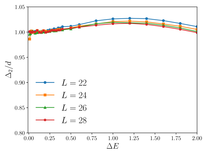
Figure S2: $\Delta_{2}/d$ versus $\Delta E$ for the operator ${\cal A}_{q=\frac{L}{2}}$. This operator, in the large system size limit, should have $L$-independent thermalization time. This behavior is difficult to observe from the available data for $\Delta_{2}$. The data confirms, that for small $\Delta E$ the ratio $\Delta_{2}/d$ is approximately constant (the plateau of $f^{2}(\omega)$). Now, if we define $\Delta E_{T}$ as the point where $\Delta_{2}/d$ deviates, say by $1\%$, from the constant value, the approximate numerical value will be $\Delta E_{T}\approx 0.3$. But since the curve of $(\Delta_{2}/d)$ changes its overall shape for growing $L$, it is conceivable that for large L the “plateau” region will extend to much large values of order $\Delta E_{T}\approx 1-1.5$.

With this definition we readily find $\Delta E_{U}^{(2)}=\Delta E_{T}$. In our numerical analysis we defined $\Delta E_{U}=\Delta E_{U}^{(4)}$ and saw that in most cases $\Delta E_{U}^{(6)}\approx\Delta E_{U}^{(4)}\ll\Delta E_{U}^{(2)}=\Delta E_{T}$. An interesting question is to understand the scaling of $\Delta E_{U}^{(k)}$ for $k\gg 1$. To this end, we introduce one more scale $\Delta E_{GUE}$ which marks the onset of Gaussian RMT universality. Gaussian RMT is characterized by vanishing higher free cumulants, $\Delta_{k}=0$, except for $k=2$. It is natural thus to define $\Delta E_{RMT}^{(k)}$, similarly to (S37), as a maximal value of $\Delta E$ within which all higher moments, properly normalized, plunge below some $\epsilon$,

$$\left|{\Delta_{k}\over(\Delta_{2})^{k/2}}\right|_{\Delta E_{RMT}}=\epsilon\ .$$ (S38)

So far the operator exhibits emergent unitary symmetry, (S20) predicts

$$\frac{\Delta_{k}}{(\Delta_{2})^{k/2}}\sim\left(\frac{d(\Delta E)}{d(\Delta E_{U}^{(k)})}\right)^{\frac{k}{2}-1}\rightarrow 0\ ,$$ (S39)

for small $\Delta E$. Thus, we immediately conclude that for any small but fixed $\epsilon$, Gaussian RMT scale $\Delta E_{GUE}^{(k)}$ will be (much) smaller, but not parametrically (in terms of system-size dependence) smaller than $\Delta E_{U}^{(k)}$.

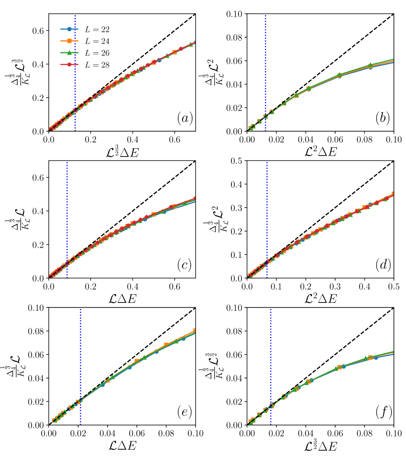
Figure S3: $\frac{\Delta_{4}^{\frac{1}{3}}}{K_{\cal L}}{\cal L}^{p}$ versus ${\cal L}^{p}\Delta E$ with the best fit values of $K_{\cal L}$ and $p$ to achieve $L$-independence (best data collapse) for (a) ${\cal A}_{q=\frac{L}{2}}$; (b) ${\cal A}_{q=1}$; (c) ${\cal B}_{q=\frac{L}{2}}$; (d) ${\cal B}_{q=1}$; (e) ${\cal B}_{q=0}$ and (f) local energy operator ${\cal A}$ (S43). Here ${\cal L}=L/24$ and use $p=\frac{n}{2}$ with integer $n$ as a tuning parameter. Inclined dashed lines (black) indicate theoretical behavior $\Delta_{k}\propto\Delta E^{k-1}$. Vertical dotted lines (blue) indicate the approximate location of $\Delta E_{U}$ as an guide to the eye.

This conclusion, combined with the result of [16] suggests a non-trivial scaling hierarchy. Indeed, by considering thermalization of the density-wave operators (of the type introduced in Eq. (11) in the main text) in 1D systems, and assuming they are coupled to conserved quantity with the sub-ballistic (e.g. diffusive) transport, Ref. [16] imposed a bound on the $\Delta E_{GUE}$ scale,

$$\Delta E_{GUE}\lesssim\Delta E_{T}/L\ .$$ (S40)

This scale has a simple physical interpretation of inverse timescale when the expectation value of $\mathcal{O}$ in some initial out-of-equilibrium state $\ket{\Psi}$ will become of order of quantum fluctuations,

$$\langle\Psi|{\mathcal{O}}(t)|\Psi\rangle\approx e^{-\Delta E_{T}t}\sim e^{-S/2}\ .$$ (S41)

The bound (S40) is based on the property of Gaussian RMT that the largest eigenvalue of the microcanonically truncated operator will grow with $\Delta E$ as $\sqrt{\Delta E}$. (This is the same as the size of Wigner’s semicircle distribution being proportional to square root of the matrix size $\sqrt{d}$.) This behavior is guaranteed, provided $\Delta_{2}^{k}$ gives leading contribution to ${\cal M}_{2k}$ (S11), or $\Delta_{2k}/(\Delta_{2})^{k}\ll 1$ for $k\gg 1$. In other words, for $k\gg 1$, $\Delta E_{GUE}^{(k)}$ obeys (S40). Combining all together we find $\Delta E_{GUE}^{(k)}\ll\Delta E_{U}^{(k)}$ while both scale with $L$ as

$$\Delta E_{T}/L\sim{q^{2}\over L^{3}}\ ,$$ (S42)

and thus parametrically smaller than $\Delta E_{T}$.

We emphasize, the system size scaling (S42) should apply to $\Delta E_{RMT}^{(k)},\Delta E_{U}^{(k)}$ with $k\gg 1$, while in our numerical analysis we used $k=4$. We leave open the question of how $\Delta E_{U}^{(k)}/\Delta E_{U}^{(l)}$ would scale with the system-size when $k\gg l$. Elucidating this question would be necessary to confirm the hierarchical behavior $\Delta E_{GUE}\ll\Delta E_{U}\ll\Delta E_{T}$ introduced in the main text.

Additional numerical results

System size dependence of $\Delta E_{U}$.

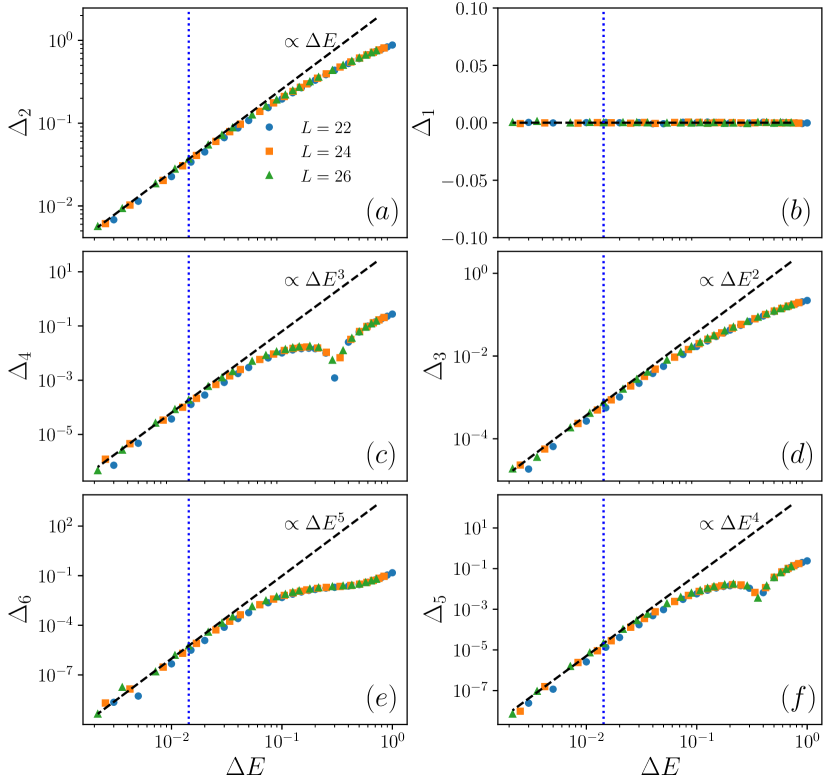
Figure S4: Free cumulants $\Delta_{k}$ versus $\Delta E$ for local operator ${\cal A}$. Inclined dashed lines (black) indicate theoretical behavior $\Delta_{k}\propto\Delta E^{k-1}$. Vertical dotted lines (blue) indicate the approximate location of $\Delta E_{U}$ for guide to the eye.

Numerically, the procedure to determine $\Delta E_{U}$ from Eq. (S37) is not very accurate. To study $L$ dependence of $\Delta E_{U}$ we employ a different approach. Considering an operator of interest, we try to find two tuning parameters $K_{L}$ and $p$ such that the curves of ${\Delta_{4}^{1/3}L^{p}\over K_{L}}$ as a function of $L^{p}\Delta E$ for different $L$ would approximately be $L$-independent. We do this in two steps. We first consider $\Delta_{4}^{\frac{1}{3}}$, which grows linearly for small $\Delta E$, and find $K_{L}^{-1}$ such that for very small $\Delta E$, $K_{L}^{-1}\Delta_{4}^{\frac{1}{3}}\approx\Delta E$. Next we find a tuning parameter $p$ to achieve best possible data collapse ($L$-independence) of $\frac{\Delta_{4}^{\frac{1}{3}}}{K_{L}}{L}^{p}$ as a function of ${L}^{p}\Delta E$. We choose $p$ in the form $p=\frac{n}{2}$ with integer $n$. For convenience instead of $L$ we use ${\cal L}=L/24$ and plot $\frac{\Delta_{4}^{\frac{1}{3}}}{K_{\cal L}}{\cal L}^{p}$ as a function of ${\cal L}^{p}\Delta E$. The results are shown in in Fig. S3, where we find $p$ to be positive for all operators considered. This suggests $\Delta E_{U}\sim L^{-p}$ scaling with positive $p$.

Our results suggest that $\Delta E_{U}\propto{\cal L}^{-p}$ with $p\geq 0$, but the precise value of $p$ is dependent on the observable of interest. While a perfect data collapse is difficult to achieve for most observables, the precise finite-size scaling of $\Delta E_{U}$ remains unclear. This should not come as a surprise, as the system sizes $L=22,\dots,28$ are likely still too small to observe the asymptotic scaling regime.

Local operators. Next we consider a local energy density operator ,

$${\cal A}=\frac{h}{2}(\sigma_{x}^{1}+\sigma_{x}^{2})+\frac{g}{2}(\sigma_{z}^{1}+\sigma_{z}^{2})+J\sigma_{z}^{1}\sigma_{z}^{2}\ .$$ (S43)

Numerical results are show in Fig. S4. Similar to the density wave operator, apart from the deviations at extremely small $\Delta E$, $\Delta_{k}\propto\Delta E^{k-1}$ behavior is observed below certain energy scale, indicating emergence of unitary symmetry at $\Delta E\leq\Delta E_{U}$.

Finally in Fig. S5, we study another local operator

$${\cal B}=h\sigma_{z}^{1}-g\sigma_{x}^{1}.$$ (S44)

Similarly, $\Delta_{k}\propto\Delta E^{k-1}$ behavior emerges within a sufficiently small energy window.

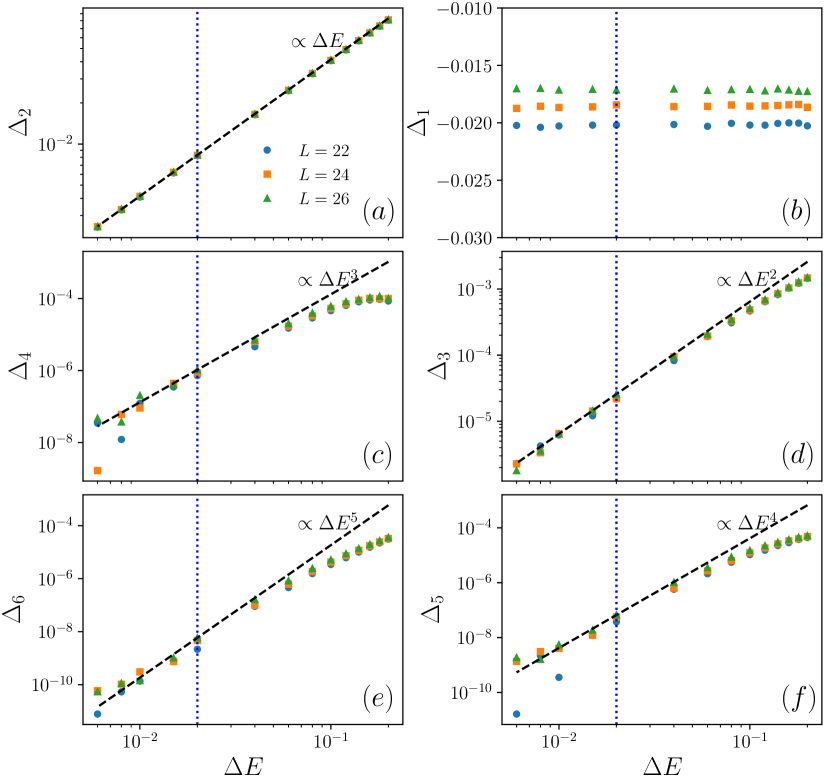
s

Figure S5: Free cumulants $\Delta_{k}$ versus $\Delta E$ for local operator ${\cal B}$. Inclined dashed lines (black) indicate theoretical behavior $\Delta_{k}\propto\Delta E^{k-1}$. Vertical dotted lines (blue) indicate the approximate location of $\Delta E_{U}$ for guide to the eye.

Details of the numerical method

The key idea of our numerical approach is the expansion of projector operator $P_{\Delta E}=\sum_{|E_{m}-E_{0}|<\Delta E/2}\ket{m}\bra{m}$ in terms of Chebyshev polynomials of the Hamiltonian given, see Eq. (S52) in the main text. In this section, we are going to explain the numerical method in more detail.

In the eigenbasis, $P_{\Delta E}$ can be written as,

$$P_{\Delta E} =\sum_{m}P(E_{m})|m\rangle\langle m|\ ,$$ (S45)

$$P_{\Delta E}(E) =\text{rect}\left(\frac{E-E_{0}}{\Delta E}\right)\ ,$$ (S46)

where $\text{rect}(x)$ indicates the rectangular function defined as,

$$\text{rect}(x)=\begin{cases}0&\text{if }|x|\geq\frac{1}{2}\\ 1&\text{if }|x|<\frac{1}{2}\end{cases}\ .$$ (S47)

The rectangular function can be expanded in terms of Chebyshev polynomials of the first kind (denoted by $T_{k}(x)$),

$$P_{\Delta E}(E)=\sum_{k=0}^{\infty}C_{k}T_{k}\left(\frac{E-b}{a}\right),$$ (S48)

where $a=(E_{\text{max}}-E_{\text{min}})/2$, $b=(E_{\text{max}}+E_{\text{min}})/2$. The coefficients $C_{k}$ are written as

$$C_{0}=\frac{1}{\pi}\left[\arcsin\left(\frac{\frac{\Delta E}{2}+b-E_{0}}{a}\right)-\arcsin\left(\frac{-\frac{\Delta E}{2}+b-E_{0}}{a}\right)\right]\ ,$$ (S49)

and

$$C_{k}(k\geq 1) =\frac{2(-1)^{k+1}}{\pi k}\biggl{[}\sin\biggl{(}k\arccos\biggl{(}\frac{\frac{\Delta E}{2}+b-E_{0}}{a}\biggl{)}\biggl{)}$$

$$-\sin\biggl{(}k\arccos\biggl{(}\frac{-\frac{\Delta E}{2}+b-E_{0}}{a}\biggl{)}\biggl{)}\biggl{]}\ .$$ (S50)

In practice, the infinite series in Eq. (S48) needs to be truncated to finite order $N_{\text{tr}}$,

$$P_{\Delta E}(E)\simeq\sum_{k=0}^{N_{\text{tr}}}C_{k}T_{k}\left(\frac{E-b}{a}\right)\ .$$ (S51)

In the following, we denote $N_{\text{tr}}$ by $N$ for simplicity. $P_{\Delta E}$ finally can be approximated as

$$P_{\Delta E}\simeq P_{\Delta E}^{(N)}\equiv\sum_{k=0}^{N}C_{k}T_{k}\left(\frac{H-b}{a}\right)\ .$$ (S52)

Applying the above equation to a Gaussian random state

$$|\psi\rangle=\sum_{i=1}^{D}c_{i}|i\rangle\ ,$$ (S53)

where $c_{i}$ is a Gaussian random number and $\ket{i}$ denote the computational basis, the $k$-th moment of an operator $\cal O$ can be approximated by relying on quantum typicality,

$${\cal M}_{k}\simeq\frac{\langle\psi|(P_{\Delta E}^{(N)}{\cal O}P_{\Delta E}^{(N)})^{k}|\psi\rangle}{\langle\psi|P_{\Delta E}^{(N)}|\psi\rangle}\ .$$ (S54)

Moreover, making use of $\left(P_{\Delta E}^{(N)}\right)^{2}\simeq P_{\Delta E}^{(N)}$, Eq. (S54) is simplified as

$${\cal M}_{k}\simeq{\cal M}_{k}^{\text{typ}}\equiv\frac{\langle\psi|P_{\Delta E}^{(N)}({\cal O}P_{\Delta E}^{(N)})^{k}|\psi\rangle}{\langle\psi|P_{\Delta E}^{(N)}|\psi\rangle}\ ,$$ (S55)

where one only needs to apply the energy filter $P_{\Delta E}^{(N)}$ for $k+1$ times, instead of $2k$ times in the original expression (S54). In the numerical simulations, to further reduce statistical errors, an additional average is taken over $N_{\text{typ}}$ different realization of random state,

$$\overline{{\cal M}_{k}^{\text{typ}}}=\frac{1}{N_{\text{typ}}}\sum_{n=1}^{N_{\text{typ}}}\frac{\langle\psi_{n}|P_{\Delta E}^{(N)}({\cal O}P_{\Delta E}^{(N)})^{k}|\psi_{n}\rangle}{\langle\psi_{n}|P_{\Delta E}^{(N)}|\psi_{n}\rangle}\ .$$ (S56)

where $|\psi_{n}\rangle$ indicates an individual realization of a Gaussian random state. The Chebyshev expansion becomes more accurate if one increases the number of terms in the expansion $N$, but the simulation time is proportional to $N$, hence larger $N$ will result in a longer simulation time. In our numerical simulations $N=100a\frac{2\pi}{\Delta E}$ which is found to yield high accuracy of results.

Error analysis

Figure S6: Comparison of $\Delta^{\text{typ}}_{k}$ (green triangle, averaged over $2^{12}$ random states), $\Delta^{\text{ch}}_{k}$ (orange square) and $\Delta_{k}$ (blue circle with solid line, calculated by ED) for operator: [(a) (c)] ${\cal A}_{q=\frac{L}{2}}$ and [(b) (d)] ${\cal A}_{q=1}$ for system size $L=16$.

In this section, we perform an error analysis of our typicality-based numerical method. The total error in our approach comes from two different sources: (i) a truncation error $\varepsilon_{\text{tr}}$ [due to the finite order $N$ in the Chebyshev expansion (S52)], and (ii) a typicality error $\varepsilon_{\text{typ}}$ [due to approximating the trace by a random state in Eq. (S54)]. The typicality error $\varepsilon_{\text{typ}}$ is easy to estimate. It scales as $\varepsilon_{\text{typ}}\sim(N_{\text{typ}}d)^{-1/2}$, where $d$ is the number of states in the energy window. In the numerical simulations, $N_{\text{typ}}$ is chosen according to the system size, $N_{\text{typ}}\propto 2^{-L}$, which then assures similar accuracy for different $L$. More precisely, the typicality error for the approximation of ${\cal M}_{k}$ is given by

$$\varepsilon_{\text{typ}}({\cal M}_{k})=\sqrt{\frac{{\cal M}_{2k}-{\cal M}_{k}^{2}}{N_{\text{typ}}d}}\ .$$ (S57)

The relative (typicality) error is given by

$$\frac{\varepsilon_{\text{typ}}({\cal M}_{k})}{|{\cal M}_{k}|}=\sqrt{\frac{{\cal M}_{2k}-{\cal M}_{k}^{2}}{{\cal M}_{k}^{2}}}\frac{1}{\sqrt{N_{\text{typ}}d}}\ .$$ (S58)

We will readily see that it depends on the order $k$. To estimate the relative error of even moments, let’s consider the case where all odd moments vanish. It is known that if an operator can be described by a GOE random matrix, one has

$${\cal M}_{2k}=\Lambda_{k}({\cal M}_{2})^{k}\ ,$$ (S59)

where $\Lambda_{k}=\frac{(2k)!}{(k+1)!k!}$ is the Catalan number. Within a small energy window $\Delta E\ll\Delta E_{U}$, $k$-th cumulant decays as $\Delta_{k}\propto{\Delta E}^{k-1}$, Eq. (S59) holds approximately, and one has

$$\frac{{\cal M}_{2k}-{\cal M}_{k}^{2}}{{\cal M}_{k}^{2}}\sim\frac{\Lambda_{k}}{\Lambda_{\frac{k}{2}}^{2}}\sim k^{\frac{3}{2}}\ ,\quad\text{for even }k\gg 2\ .$$ (S60)

As a result one has the following estimation for even moments

$$\frac{\varepsilon_{\text{typ}}({\cal M}_{k})}{|{\cal M}_{k}|}\sim k^{\frac{3}{4}}\frac{1}{\sqrt{N_{\text{typ}}d}}\ ,$$ (S61)

indicating that the relative error of ${\cal M}_{k}$ increases as a power law in $k$. For the density-wave operators with non-zero wave number, odd moments approximately vanish. So in our numerical simulation, we neglect all the odd moments and only even moments are considered. For all other operators, for which the odd moments are not negligibly small, the ratio $\frac{{\cal M}_{2k}-{\cal M}_{k}^{2}}{{\cal M}_{k}^{2}}$ is operator-dependent. Usually we expect that $\frac{{\cal M}_{2k}-{\cal M}_{k}^{2}}{{\cal M}_{k}^{2}}$ increase with $k$, which leads to a larger relative error for higher moments. It should be mentioned here that, as free cumulants $\Delta_{k}$ are calculated by making use of moments ${\cal M}_{k}$, their relative error are in general larger than that of ${\cal M}_{k}$.

Figure S7: Comparison of result of $\Delta_{k}$ from single precision $\Delta^{\text{sp}}_{k}$ (blue circle) and double precision $\Delta^{\text{sp}}_{k}$ (red square) simulations, for operator: [(a) (c)] ${\cal A}_{q=\frac{L}{2}}$ and [(b) (d)] ${\cal A}_{q=1}$ for system size $L=24$. The result is obtained from a single random state.

The truncation error $\varepsilon_{\text{tr}}$ depends on the number of Chebyshev polynomials we keep in the expansion of Eq. (S52). Different from the typicality error, an analytical expression of truncation error is very hard to derive. We try to estimate $\varepsilon_{\text{tr}}$ numerically instead. To this end, we consider

$${\cal M}_{k}^{\text{ch}}\equiv\frac{\text{Tr}\left[P_{\Delta E}^{(N)}({\cal O}P_{\Delta E}^{(N)})^{k}\right]}{\text{Tr}\left[P_{\Delta E}^{(N)}\right]}\ .$$ (S62)

It can be easily seen that ${\cal M}_{k}^{\text{ch}}\to{\cal M}_{k}$ for $N\rightarrow\infty$ and $\overline{{\cal M}_{k}^{\text{typ}}}\to{\cal M}_{k}^{\text{ch}}$ if the Hilbert-space dimension is sufficiently large or if the results are averaged over many realizations of random state. Here $\overline{{\cal M}_{k}^{\text{typ}}}$ indicates that the trace is approximated by random states. We denote the cumulants calculated by $\overline{{\cal M}_{k}^{\text{typ}}}$ and ${\cal M}_{k}^{\text{ch}}$ as $\Delta^{\text{typ}}_{k}$ and $\Delta^{\text{ch}}_{k}$, respectively. The error $\varepsilon_{\text{typ}}$ and $\varepsilon_{\text{tr}}$ can be probed by

$$\varepsilon_{\text{tr}}\propto|\Delta_{k}^{\text{ch}}-\Delta_{k}|\ ,\quad\varepsilon_{\text{typ}}\propto|\Delta_{k}^{\text{ch}}-\Delta_{k}^{\text{typ}}|\ .$$ (S63)

We compare $\Delta^{\text{typ}}_{k}$, $\Delta^{\text{ch}}_{k}$ and $\Delta_{k}$ for system size $L=16$ in Fig. S6 . For the operators considered, a neat agreement between $\Delta_{k}^{\text{ch}}$ and $\Delta_{k}$ can be seen, indicating a small truncation error $\varepsilon_{\text{tr}}$. $\Delta_{k}^{\text{typ}}$ (calculated by averaging over $2^{12}$ random states) also remains very close to $\Delta_{k}^{\text{ch}}$ for almost all $\Delta E$, indicating a small typicality error $\varepsilon_{\text{typ}}$. Deviations can be observed for $\Delta E\rightarrow 0$, especially for $\Delta_{6}$ of ${\cal A}_{q=\frac{L}{2}}$ [Fig. S6 (b)] when the number of states within the energy window plunges below $d\lesssim 1000$.

It should be mentioned here that all our numerical simulations with the typicality-based method are done in single precision. The accuracy of single precision simulation is checked in several observables (see Fig. S7), where we find that the difference between results from single and double precision simulations are neglectably small.

References

- [1] L. D’Alessio,Y. Kafri, A. Polkovnikov, and M. Rigol, From quantum chaos and eigenstate thermalization to statistical mechanics and thermodynamics, Adv. Phys. 65, 239 (2016).
- [2] A. Dymarsky, N. Lashkari, and H. Liu, Subsystem eigenstate thermalization hypothesis, Phys. Rev. E 97, 012140 (2018).
- [3] S. Pappalardi, L. Foini, and J. Kurchan, Eigenstate Thermalization Hypothesis and Free Probability, Phys. Rev. Lett. 129, 170603 (2022).
- [4] M. Srednicki, The approach to thermal equilibrium in quantized chaotic systems, J. Phys. A 32, 1163 (1999).
- [5] A. Dymarsky and H. Liu, New characteristic of quantum many-body chaotic systems, Phys. Rev. E 99, 010102 (2019).
- [6] A. Dymarsky, Mechanism of macroscopic equilibration of isolated quantum systems, Phys. Rev. B 99, 224302 (2019).
- [7] A. Dymarsky, Bound on Eigenstate Thermalization from Transport, Phys. Rev. Lett. 128, 190601 (2022).
- [8] J. Richter, A. Dymarsky, R. Steinigeweg, and J. Gemmer, Eigenstate thermalization hypothesis beyond standard indicators: Emergence of random-matrix behavior at small frequencies, Phys. Rev. E 102, 042127 (2020).
- [9] J. Wang, M. Lamann, J. Richter, R. Steinigeweg, A. Dymarsky, and J. Gemmer, Eigenstate Thermalization Hypothesis and Its Deviations from Random-Matrix Theory beyond the Thermalization Time, Phys. Rev. Lett. 128, 180601 (2022).
- [10] S. Pappalardi, L. Foini, and J. Kurchan, Microcanonical windows on quantum operators, arXiv:2304.10948 (2023).
- [11] F. Iniguez and M. Srednicki, Microcanonical Truncations of Observables in Quantum Chaotic Systems, arXiv:2305.15702 (2023).
- [12] See supplemental material for details on random unitary projectors and our derivation of Eq. (10), additional numerical results, our definition of different energy scales, and details on our numerical approach. Supplemental material includes Refs. [14, 15, 16, 17, 18].
- [13] M. Fava, J. Kurchan and S. Pappalardi, Designs via Free Probability, arXiv:2308.06200 (2023).
- [14] P. Forrester, Quantum conductance problems and the Jacobi ensemble, J. Phys. A: Math. Gen. 39, 6861 (2006).
- [15] D. Savin, H. Sommers, and W. Wieczorek, Nonlinear statistics of quantum transport in chaotic cavities, Phys. Rev. B 77, 125332 (2008).
- [16] P. Vidal and E. Kanzieper, Statistics of reflection eigenvalues in chaotic cavities with nonideal leads, Phys. Rev. Lett. 108, 206806 (2012).
- [17] Z. Puchala and J. Miszczak, Symbolic integration with respect to the Haar measure on the unitary groups, Bull. Pol. Acad. Sci. Tech. Sci. 65, 21 (2017).
- [18] J. C. Osborn and J. J. M. Verbaarschot, Thouless energy and correlations of QCD Dirac eigenvalues, Nucl. Phys. B 525, 738 (1998).
- [19] L. Foini and J. Kurchan, Eigenstate Thermalization and Rotational Invariance in Ergodic Quantum Systems, Phys. Rev. Lett. 123, 260601 (2019).
- [20] B. Altshuler and B. Shklovskii, Repulsion of energy levels and conductivity of small metal samples, Sov. Phys. JETP 64, 127 (1986).
- [21] A. Friedman, A. Chan, A. De Luca, and J. Chalker, Spectral Statistics and Many-Body Quantum Chaos with Conserved Charge, Phys. Rev. Lett. 123, 210603 (2019).
- [22] M. Winer, and B. Swingle, Hydrodynamic Theory of the Connected Spectral form Factor, Phys. Rev. X 12, 021009 (2022).
- [23] M. Winer, and B. Swingle, Spontaneous symmetry breaking, spectral statistics, and the ramp, Phys. Rev. B 105, 104509 (2022).
- [24] M. Winer, and B. Swingle, Emergent Spectral Form Factors in Sonic Systems, arXiv:2211.09134 (2023).
- [25] M. Winer, and B. Swingle, Reappearance of Thermalization Dynamics in the Late-Time Spectral Form Factor, arXiv:2307.14415 (2023).
- [26] D. Roy and T. Prosen, Random matrix spectral form factor in kicked interacting fermionic chains, Phys. Rev. E 102, 060202(R) (2020).
- [27] D. Roy, D. Mishra, and T. Prosen, Spectral form factor in a minimal bosonic model of many-body quantum chaos, Phys. Rev. E 106, 024208 (2022).
- [28] V. Kumar and D. Roy Many-body quantum chaos in mixtures of multiple species, arXiv:2310.06811 (2023).
- [29] S. Pappalardi, F. Fritzsch and T. Prosen, General Eigenstate Thermalization via Free Cumulants in Quantum Lattice Systems, arXiv:2303.00713 (2023).
- [30] M. C. Bañuls, J. I. Cirac, and M. B. Hastings, Strong and Weak Thermalization of Infinite Nonintegrable Quantum Systems, Phys. Rev. Lett. 106, 050405 (2011).
- [31] J. F. Rodriguez-Nieva, C. Jonay, and Vedika Khemani, Quantifying quantum chaos through microcanonical distributions of entanglement, arXiv:2305.11940 (2023).
- [32] T. Heitmann, J. Richter, D. Schubert, and R. Steinigeweg, Selected applications of typicality to real-time dynamics of quantum many-body systems, Z. Naturforsch. 75, 421 (2020).
- [33] F. Jin, D. Willsch, M. Willsch, H. Lagemann, K. Michielsen, and H. De Raedt, Random State Technology, J. Phys. Soc. Jpn. 90, 012001 (2021).
- [34] A. Belin, J. de Boer, and D. Liska, Non-Gaussianities in the statistical distribution of heavy OPE coefficients and wormholes, JHEP 06, 116 (2022).
- [35] T. Anous, A. Belin, J. de Boer, and D. Liska, OPE statistics from higher-point crossing, JHEP 06, 102 (2022).
- [36] D. L. Jafferis, D. K. Kolchmeyer, B. Mukhametzhanov, and J. Sonner, Matrix Models for Eigenstate Thermalization, Phys. Rev. X 13, 031033 (2023).
- [37] D. L. Jafferis, D. K. Kolchmeyer, B. Mukhametzhanov, and J. Sonner, Jackiw-Teitelboim gravity with matter, generalized eigenstate thermalization hypothesis, and random matrices, Phys. Rev. D 108, 066015 (2023).
- [38] A. Belin, J. de Boer, D. L. Jafferis, P. Nayak, and J. Sonner, Approximate CFTs and Random Tensor Models, arXiv:2308.03829 (2023).
- [39] L. Foini and J. Kurchan, The Eigenstate Thermalization Hypothesis and Out of Time Order Correlators, Phys. Rev. E 99, 042139 (2019).
- [40] A. Chan, A. De Luca and J. T. Chalker, “Eigenstate Correlations, Thermalization and the Butterfly Effect,” Phys. Rev. Lett. 122 (2019) no.22, 220601, arXiv:1810.11014.
- [41] C. Murthy and M. Srednicki, Bounds on chaos from the eigenstate thermalization hypothesis, Phys. Rev. Lett. 123, 230606 (2019).
- [42] M. Brenes, S. Pappalardi, M. T. Mitchison, J. Goold, and A. Silva, Out-of-time-order correlations and the fine structure of eigenstate thermalisation, Phys. Rev. E 104, 034120 (2021).
- [43] D. Hahn, D. J. Luitz, and J. T. Chalker, The statistical properties of eigenstates in chaotic many-body quantum systems, arXiv:2309.12982 (2023).
- [44] O. Bohigas, M. J. Giannoni, and C. Schmit, Characterization of Chaotic Quantum Spectra and Universality of Level Fluctuation Laws, Phys. Rev. Lett. 52, 1 (1984).

References

- [1] P. Forrester, Quantum conductance problems and the Jacobi ensemble, J. Phys. A: Math. Gen. 39, 6861 (2006).
- [2] D. Savin, H. Sommers, and W. Wieczorek, Nonlinear statistics of quantum transport in chaotic cavities, Phys. Rev. B 77, 125332 (2008).
- [3] P. Vidal and E. Kanzieper, Statistics of reflection eigenvalues in chaotic cavities with nonideal leads, Phys. Rev. Lett. 108, 206806 (2012).
- [4] Z. Puchala and J. Miszczak, Symbolic integration with respect to the Haar measure on the unitary groups, Bull. Pol. Acad. Sci. Tech. Sci. 65, 21 (2017).
- [5] S. Pappalardi, L. Foini, and J. Kurchan, Eigenstate Thermalization Hypothesis and Free Probability, Phys. Rev. Lett. 129, 170603 (2022).
- [6] S. Pappalardi, F. Fritzsch and T. Prosen, General Eigenstate Thermalization via Free Cumulants in Quantum Lattice Systems, arXiv:2303.00713 (2023).
- [7] M. Srednicki, The approach to thermal equilibrium in quantized chaotic systems, J. Phys. A 32, 1163 (1999).
- [8] L. Foini and J. Kurchan, Eigenstate Thermalization and Rotational Invariance in Ergodic Quantum Systems, Phys. Rev. Lett. 123, 260601 (2019).
- [9] O. Bohigas, M. J. Giannoni, and C. Schmit, Characterization of Chaotic Quantum Spectra and Universality of Level Fluctuation Laws, Phys. Rev. Lett. 52, 1 (1984).
- [10] B. Altshuler and B. Shklovskii, Repulsion of energy levels and conductivity of small metal samples, Sov. Phys. JETP 64, 127 (1986).
- [11] A. Friedman, A. Chan, A. De Luca, and J. Chalker, Spectral Statistics and Many-Body Quantum Chaos with Conserved Charge, Phys. Rev. Lett. 123, 210603 (2019).
- [12] M. Winer, and B. Swingle, Hydrodynamic Theory of the Connected Spectral form Factor, Phys. Rev. X 12, 021009 (2022).
- [13] M. Winer, and B. Swingle, Spontaneous symmetry breaking, spectral statistics, and the ramp, Phys. Rev. B 105, 104509 (2022).
- [14] M. Winer, and B. Swingle, Emergent Spectral Form Factors in Sonic Systems, arXiv:2211.09134 (2023).
- [15] M. Winer, and B. Swingle, Reappearance of Thermalization Dynamics in the Late-Time Spectral Form Factor, arXiv:2307.14415 (2023).
- [16] A. Dymarsky, Bound on Eigenstate Thermalization from Transport, Phys. Rev. Lett. 128, 190601 (2022).
- [17] J. C. Osborn and J. J. M. Verbaarschot, Thouless energy and correlations of QCD Dirac eigenvalues, Nucl. Phys. B 525, 738 (1998).