Cayley Linear–Time Computable Groups

Abstract

This paper looks at the class of groups admitting normal forms for which the right multiplication by a group element is computed in linear time on a multi–tape Turing machine. We show that the groups $\mathbb{Z}_{2}\wr\mathbb{Z}^{2}$, $\mathbb{Z}_{2}\wr\mathbb{F}_{2}$ and Thompson’s group $F$ have normal forms for which the right multiplication by a group element is computed in linear time on a $2$–tape Turing machine. This refines the results previously established by Elder and the authors that these groups are Cayley polynomial–time computable.

Keywords     Cayley linear–time computable group, multi–tape Turing machine, wreath product, Thompson’s group

1 Introduction

Extensions of the notion of an automatic group introduced by Thurston and others [10] have been studied by different researchers. One of the extensions is the notion of a Cayley automatic group introduced by Kharlampovich, Khoussainov and Miasnikov [14]. In their approach a normal form is defined by a bijection between a regular language and a group such that the right multiplication by a group element is recognized by a two–tape synchronous automaton. Elder and the authors looked at the further extension of Cayley automatic groups allowing the language of normal forms to be arbitrary (though it is always recursively enumerable [2, Theorem 3]) but requiring the right multiplication by a group element to be computed by an automatic function (a function that can be computed by a two–tape synchronous automaton). This extension is referred to as Cayley position–faithful one–tape linear–time computable groups [2, Definition 3]. These groups admit quasigeodesic normal forms (see Definition 3) for which the right multiplication by a group element is computed in linear time (on a position–faithful one–tape Turing machine) and the normal form is computed in quadratic time [2, Theorem 2].

In this paper we look at the groups admitting normal forms for which the right multiplication by a group element is computed in linear time on a multi–tape Turing machine (we refer to such groups as Cayley linear–time computable). These normal forms are not necessarily quasigeodesic, see, e.g., the normal form of $\mathbb{Z}_{2}\wr\mathbb{Z}^{2}$ considered in Section 3. However, if such normal form is quasigeodesic, then it is computed in quadratic time (see Theorem 5), thus, fully retaining the basic algorithmic properties of normal forms for Cayley automatic groups: computability of the right multiplication by a group element in linear time and normal form in quadratic time. Cayley linear–time computable groups form a subset of Cayley polynomial–time computable groups introduced in [2, Definition 5], but clearly include all Cayley position–faithful one–tape linear–time computable groups. We show that the groups $\mathbb{Z}_{2}\wr\mathbb{Z}^{2}$, $\mathbb{Z}_{2}\wr\mathbb{F}_{2}$ and Thompson’s group $F$ are Cayley linear–time computable (on a $2$–tape Turing machine) which refines the previous claims that these groups are Cayley polynomial–time computable [2]. To show that these three groups are Cayley linear–time computable we use the normal forms previously studied by the second author and Khoussainov for groups $\mathbb{Z}_{2}\wr\mathbb{Z}^{2}$ and $\mathbb{Z}_{2}\wr\mathbb{F}_{2}$ [3] and Elder and Taback for Thompson’s group $F$ [9]. We note that [3, Theorems 5, 8] and [9, Theorem 3.6] showing that $\mathbb{Z}_{2}\wr\mathbb{F}_{2}$, $\mathbb{Z}_{2}\wr\mathbb{Z}^{2}$ and Thompson’s group $F$ are context–free, indexed and deterministic non–blind 1–counter graph automatic, respectively, do not imply that the right multiplications by a group element for the normal forms considered in these groups are computed in linear time on a $2$–tape Turing machine. The latter requires careful verification that is done in this paper.

Several researchers studied extensions of automatic groups utilizing different computational models. Bridson and Gilman considered an extension of asynchronously automatic groups using indexed languages [4]. Baumslag, Shapiro and Short extended the notion of an automatic group based on parallel computations by pushdown automata [1]. Brittenham and Hermiller introduced autostackable groups which also extends the notion of an automatic group [5]. Elder and Taback introduced $\mathcal{C}$–graph automatic groups extending Cayley automatic groups and studied them for different classes of languages $\mathcal{C}$ [8]. Jain, Khoussainov and Stephan introduced the class of a semiautomatic groups [12] which generalizes the notion of a Cayley automatic group. Jain, Moldagaliyev, Stephan and Tran studied extensions of Cayley automatic groups using transducers and tree automata [13].

The paper is organized as follows. In Section 2 we introduce the notion of a Cayley $k$–tape linear–time computable group. In Sections 3, 4 and 5 we show that the wreath products $\mathbb{Z}_{2}\wr\mathbb{Z}^{2}$, $\mathbb{Z}_{2}\wr\mathbb{F}_{2}$ and Thompson’s group $F$, respectively, are Cayley $2$–tape linear–time computable. Section 6 concludes the paper. Section 7 (Appendix) contains a proof of Theorem 4.

2 Preliminaries

In this section we introduce the notion of a Cayley linear–time computable group. We start with defining a basic concept underlying this notion – a function computed on a position–faithful $k$–tape Turing machine in linear time, where $k$ is a positive integer.

Definition 1.

A position–faithful $k$–tape Turing machine is a Turing machine with $k$ semi–infinite tapes for each of which the leftmost position contains the special symbol $\boxplus$ which only occurs at this position and cannot be modified. We denote by $\boxdot$ a special blank symbol, by $\Sigma$ the input alphabet for which $\Sigma\cap\{\boxplus,\boxdot\}=\varnothing$ and by $\Gamma$ the tape alphabet for which $\Sigma\cup\{\boxplus,\boxdot\}\subseteq\Gamma$. Initially, for the input $x\in\Sigma^{*}$, the configuration of the first tape is $\boxplus x\boxdot^{\infty}$ with the head being at the $\boxplus$ symbol. The configurations of other $k-1$ tapes are $\boxplus\boxdot^{\infty}$ with the head pointing at the $\boxplus$ symbol. During the computation the Turing machine operates as usual, reading and writing symbols from $\Gamma$ in cells to the right of the $\boxplus$ symbol.

A function $f:\Sigma^{*}\rightarrow\Sigma^{*}$ is said to be computed on a position–faithful $k$–tape Turing machine in linear time, if for the input string $x\in\Sigma^{*}$ of length $n$ when started with the first tape content being $\boxplus x\boxdot^{\infty}$ and other tapes content being $\boxplus\boxdot^{\infty}$, the heads pointing at $\boxplus$, the Turing machine reaches an accepting state and halts in $Cn$ or fewer steps with the first tape having prefix $\boxplus f(x)\boxdot$, where $C>0$ is a constant. There is no restriction on the output beyond the first appearance of $\boxdot$ on the first tape, the content of other tapes and the positions of their heads.

In Definition 1 position–faithfulness refers to a way the output in $\Sigma^{*}$ computed on a Turing machine is defined: it is the string $v\in\Sigma^{*}$ for which the content of the first tape after a Turing machine halts is $\boxplus v\boxdot w\boxdot^{\infty}$, where $w$ is some string in $\Gamma^{*}$. In general the output in $\Sigma^{*}$ computed on a Turing machine can be defined as the content of the first tape after it halts with all symbols in $\Gamma\setminus\Sigma$ removed: see [15] where the output of the computation on a one–tape Turing machine is defined as the string $y\in\Gamma^{*}$ for which the content of the tape after it halts is $\boxplus y\boxdot^{\infty}$, where $y$ is either empty or the last symbol of $y$ is not $\boxdot$. For $k=1$ the restriction to position–faithful Turing machine matters – there exist functions computed in linear time on a one–tape Turing machine which cannot be computed in linear time on a position–faithful one–tape Turing machine [7]. The latter is due to the fact that shifting may require quadratic time. For $k>1$ the restriction to position–faithful Turing machines becomes irrelevant as shifting can always be done in linear time. Therefore, for $k>1$, we will simply say that a function if computed on a $k$–tape Turing machine in linear time omitting the term position–faithful. Recall that a function $f:\Sigma^{*}\rightarrow\Sigma^{*}$ is called automatic if the language of convolutions $L_{f}=\{u\otimes v\,|\,u,v\in\Sigma^{*}\}$ is regular. Case, Jain, Seah and Stephan showed that $f:\Sigma^{*}\rightarrow\Sigma^{*}$ is computed on a position–faithful $1$–tape Turing machine in linear time if and only if it is automatic [7]. For $k>1$ the class of functions computed on $k$–tape Turing machines in linear time is clearly wider than the class of automatic functions.

Now let $G$ be a finitely generated group. Let $S=\{s_{1},\dots,s_{k}\}\subset G$ be a set of its semigroup generators. That is, every group element of $G$ can be written as a product of elements in $S$. Below we define Cayley linear–time computable groups.

Definition 2.

We say that $G$ is Cayley position–faithful $k$–tape linear–time computable if there exist a language $L\subseteq\Sigma^{*}$, a bijective mapping $\psi:L\rightarrow G$ and functions $f_{s}:\Sigma^{*}\rightarrow\Sigma^{*}$, for $s\in S$, each of which is computed on a position–faithful $k$–tape Turing machine in linear time, such that for every $w\in L$ and $s\in S$: $\psi(f_{s}(w))=\psi(w)s$. That is, the following diagram commutes:

$$\leavevmode\hbox to52.78pt{\vbox to41.77pt{\text{[drawing]}}}, {L} {L} {G} {G} \scriptstyle{f_{s}} \scriptstyle{\psi} \scriptstyle{\psi} \scriptstyle{r_{s}} {L} {L} {G} {G} \scriptstyle{f_{s}} \scriptstyle{\psi} \scriptstyle{\psi} \scriptstyle{r_{s}}$$

where $r_{s}:G\rightarrow G$ is the right multiplication by $s$ in $G$: $r_{s}(g)=gs$ for all $g\in G$.

We refer to a bijective mapping $\psi:L\rightarrow G$ as representation. It defines a normal form of a group $G$ which for every group element $g\in G$ assigns a unique string in $w\in L$ such that $\psi(w)=g$. For the latter we also say that $w$ is a normal form of a group element $g$. We will say that a representation $\psi:L\rightarrow G$ from Definition 2, as well as the corresponding normal form of $G$, are position–faithful $k$–tape linear–time computable. We note that Definition 2 does not depend on the choice of a set of semigroup generators $S$ – this follows directly from the observation that a composition of functions computed on position–faithful $k$–tape Turing machines in linear time is also computed on a position–faithful $k$–tape Turing machine in linear time. For $k>1$ we will simply say that a group is Cayley $k$–tape linear–time computable omitting the term position–faithful. Similarly, we will say that a representation (a normal form) is $k$–tape linear–time computable (or multi–tape linear–time computable if the number of tapes is not specified).

Cayley position–faithful one–tape linear–time computable groups were studied in [2]. They comprise wide classes of groups (e.g., all polycyclic groups), but at the same time retain all basic properties of Cayley automatic groups. Namely, each of such groups admits a normal form for which the right multiplication by a fixed group element is computed in linear time and for a given word $g_{1}\dots g_{n}$, $g_{i}\in S$, the normal form of $g=g_{1}\dots g_{n}$ is computed in quadratic time. Furthermore, a position–faithful one–tape linear–time computable normal form is always quasigeodesic [2, Theorem 1]; see the notion of a quasigeodesic normal form introduced by Elder and Taback [8, Definition 4]:

Definition 3.

A representation $\psi:L\rightarrow G$ (a normal form of $G$) is said to be quasigeodesic if there exists a constant $C>0$ such that for all $g\in G$: $|w|\leqslant C(d_{S}(g)+1)$, where $w$ is the normal form of $g$, $|w|$ is its length and $d_{S}(g)$ is the length of a shortest word $g_{1}\dots g_{n}$, $g_{i}\in S$, for which $g=g_{1}\dots g_{n}$ in $G$.

Moreover, this statement can be generalized to the following theorem.

Theorem 4.

A one–tape $o(n\log n)$–time computable normal form is quasigeodesic.

Proof.

See Section 7 (Appendix) for the proof. ∎

If $k>1$, a $k$–tape linear–time computable normal form is not necessarily quasigeodesic: in Section 3 we show that the normal form of the wreath product $\mathbb{Z}_{2}\wr\mathbb{Z}^{2}$ constructed in [3, Section 5] is $2$–tape linear–time computable; but this normal form is not quasigeodesic [3, Remark 9]. However, if a $k$–tape linear–time computable normal form is quasigeodesic, then it satisfies the same basic algorithmic property as a position–faithful one–tape linear–time computable normal form – it is computed in quadratic time [2, Theorem 2]. Indeed, let $\psi:L\rightarrow G$ be a bijection between a language $L\subseteq\Sigma^{*}$ and a group $G$ defining a quasigeodesic $k$–tape linear–time computable normal form of $G$. Let $S\subset G$ be a finite set of semigroup generators.

Theorem 5.

There is a quadratic–time algorithm which for a given word $g_{1}\dots g_{n}\in S^{*}$, $g_{i}\in S$, computes the normal form of the group element $g=g_{1}\dots g_{n}\in G$ – the string $w\in L$ for which $\psi(w)=g$.

Proof.

Let $w_{i}\in L$ be the normal form of the group element $g_{1}\dots g_{i}$: $\psi(w_{i})=g_{1}\dots g_{i}$ for $i=1,\dots,n$. Let $w_{0}$ be the normal form of the identity: $\psi(w_{0})=e$. For each $i=0,\dots,n-1$, the string $w_{i+1}$ is computed from $w_{i}$ on a $k$–tape Turing machine in $O(|w_{i}|)$ time. Since the normal form is quasigeodesic, $|w_{i}|\leqslant C(i+1)$ for all $i=0,\dots,n-1$. So $w_{i+1}$ is computed from $w_{i}$ in $O(i)$ time for all $i=0,\dots,n-1$. Now an algorithm computing $w$ from a given input $g_{1}\dots g_{n}$ is as follows. Starting from $w_{0}$ it consecutively computes $w_{1},w_{2},\dots,w_{n-1}$ and $w_{n}$. The running time for this algorithm is at most $O(n^{2})$. ∎

As an immediate corollary of Theorem 5 we obtain that the word problem for a group $G$ which admits a quasigeodesic $k$–tape linear–time computable normal form is decidable in quadratic time.

3 The Wreath Product $\mathbb{Z}_{2}\wr\mathbb{Z}^{2}$

In this section we will show that the group $\mathbb{Z}_{2}\wr\mathbb{Z}^{2}$ is Cayley $2$–tape linear–time computable. Every group element of $\mathbb{Z}_{2}\wr\mathbb{Z}^{2}$ can be written as a pair $(f,z)$, where $z\in\mathbb{Z}^{2}$ and $f:\mathbb{Z}^{2}\rightarrow\mathbb{Z}_{2}$ is a function for which $f(\xi)$ is the non–identity element of $\mathbb{Z}_{2}$ for at most finitely many $\xi\in\mathbb{Z}^{2}$. We denote by $c$ the non–identity element of $\mathbb{Z}_{2}$ and by $a=(1,0)$ and $b=(0,1)$ the generators of $\mathbb{Z}^{2}=\{(x,y)\,|\,x,y\in\mathbb{Z}\}$. The group $\mathbb{Z}_{2}$ is canonically embedded in $\mathbb{Z}_{2}\wr\mathbb{Z}^{2}$ by mapping $c$ to $(f_{c},e)$, where $f_{c}:\mathbb{Z}^{2}\rightarrow\mathbb{Z}_{2}$ is a function for which $f_{c}(z^{\prime})=e$ for all $z^{\prime}\neq e$ and $f_{c}(e)=c$. The group $\mathbb{Z}^{2}$ is canonically embedded in $\mathbb{Z}_{2}\wr\mathbb{Z}^{2}$ by mapping $z\in\mathbb{Z}^{2}$ to $(f_{e},z)$, where $f_{e}(z^{\prime})=e$ for all $z^{\prime}\in\mathbb{Z}^{2}$. Therefore, we can identify $a,b$ and $c$ with the corresponding group element $(f_{e},a)$, $(f_{e},b)$ and $(f_{c},e)$ in $\mathbb{Z}_{2}\wr\mathbb{Z}^{2}$, respectively. The group $\mathbb{Z}_{2}\wr\mathbb{Z}^{2}$ is generated by $a,b$ and $c$, so $S=\{a,a^{-1},b,b^{-1},c\}$ is a set of its semigroup generators. The formulas for the right multiplication in $\mathbb{Z}_{2}\wr\mathbb{Z}^{2}$ by $a$, $a^{-1}$, $b$, $b^{-1}$ and $c$ are as follows. For a given $g=(f,z)\in\mathbb{Z}_{2}\wr\mathbb{Z}^{2}$, where $z=(x,y)$, $ga=(f,z_{1})$ for $z_{1}=(x+1,y)$, $ga^{-1}=(f,z_{1}^{\prime})$ for $z_{1}^{\prime}=(x-1,y)$, $gb=(f,z_{2})$ for $z_{2}=(x,y+1)$, $gb^{-1}=(f,z_{2}^{\prime})$ for $z_{2}^{\prime}=(x,y-1)$ and $gc=(f^{\prime},z)$, where $f^{\prime}(z^{\prime})=f(z^{\prime})$ for all $z^{\prime}\neq z$ and $f^{\prime}(z)=f(z)c$.

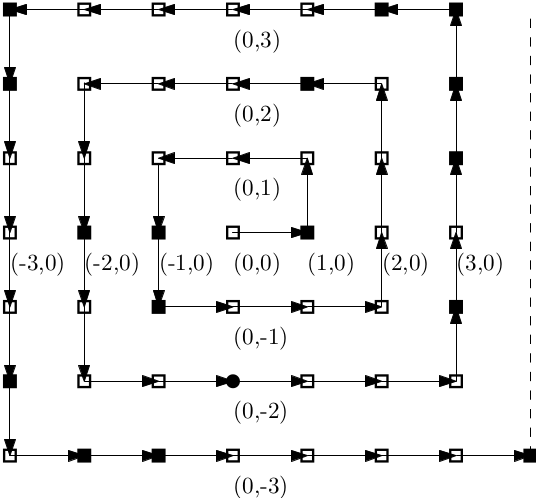
Figure 1: An infinite digraph $\Gamma$ and an element $h\in\mathbb{Z}_{2}\wr\mathbb{Z}^{2}$.

Normal form. We will use a normal form for elements of $\mathbb{Z}_{2}\wr\mathbb{Z}^{2}$ described in [3]. Let $\Gamma$ be an infinite directed graph shown on Fig. 1 which is isomorphic to $\left(\mathbb{N};\mathrm{S}\right)$, where $\mathrm{S}:\mathbb{N}\rightarrow\mathbb{N}$ is the successor function $\mathrm{S}(n)=n+1$. The vertices of $\Gamma$ are identified with elements of $\mathbb{Z}^{2}$; each vertex of $\Gamma$, except $(0,0)$, has exactly one ingoing and one outgoing edges and the vertex $(0,0)$ has one outgoing edge and no ingoing edges. Let $t:\mathbb{N}\rightarrow\mathbb{Z}^{2}$ be a mapping defined as follows: $t(1)=(0,0)$ and, for $k>1$, $t(k)=(x,y)$ is the end vertex of a directed path in $\Gamma$ of length $k-1$ which starts at the vertex $(0,0)$.

We denote by $\Sigma$ the alphabet $\Sigma=\{0,1,C_{0},C_{1}\}$. Let $g=(f,z)$ be an element of the group $\mathbb{Z}_{2}\wr\mathbb{Z}^{2}$. We denote by $r$ a number for which $t(r)=z$. Let $m=\max\{k\,|\,f(t(k))=1\}$ and $\ell=\max\{m,r\}$. A normal form $w\in\Sigma^{*}$ of the group element $g$ is defined to be a string $w=\sigma_{1}\dots\sigma_{\ell}$ of length $\ell$ for which $\sigma_{k}=0$, if $f(t(k))=0$ and $k\neq r$, $\sigma_{k}=1$ if $f(t(k))=1$ and $k\neq r$, $\sigma_{k}=C_{0}$ if $f(t(k))=0$ and $k=r$, $\sigma_{k}=C_{1}$ if $f(t(k))=1$ and $k=r$. For an illustration consider a group element $h\in\mathbb{Z}_{2}\wr\mathbb{Z}^{2}$ shown on Fig. 1: a white square indicates that the value of a function $f$ at a given point is $e$, a black square indicates that it is $c$, a black disk at the point $p=(0,-2)$ indicates that $f(p)=c$ and it specifies the position of the lamplighter. A normal form of the group element $h$ is the string: $0100011000000100001000C_{1}000101111000011000101100001$.

We denote by $L\subseteq\Sigma^{*}$ a language of all such normal forms. The described normal form of $\mathbb{Z}_{2}\wr\mathbb{Z}^{2}$ defines a bijection $\psi:L\rightarrow\mathbb{Z}_{2}\wr\mathbb{Z}^{2}$ mapping $w\in L$ to the corresponding group element $g\in\mathbb{Z}_{2}\wr\mathbb{Z}^{2}$. This normal form is not quasigeodesic [3, Remark 9].

Construction of Turing machines computing the right multiplication in $\mathbb{Z}_{2}\wr\mathbb{Z}^{2}$ by $a^{\pm 1},b^{\pm 1}$ and $c$. For the right multiplication in $\mathbb{Z}_{2}\wr\mathbb{Z}^{2}$ by $c$, consider a one–tape Turing machine which reads the input $u\in\Sigma^{*}$ from left to right and when the head reads a symbol $C_{0}$ or $C_{1}$ it changes it to $C_{1}$ or $C_{0}$, respectively, and then it halts. If the head reads the blank symbol $\boxdot$, which indicates that the input $u$ has been read, it halts. The described Turing machine halts in linear time for every input $u\in\Sigma^{*}$. Moreover, if the input $u\in L$, it computes the output $v\in L$ for which $\psi(u)c=\psi(v)$.

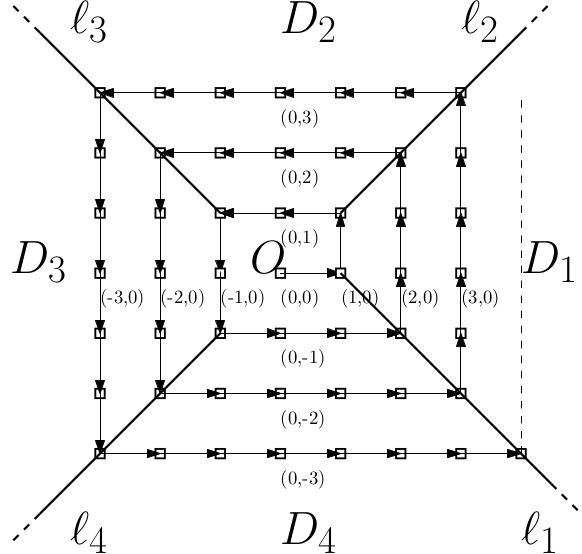
Figure 2: A digraph $\Gamma$ and subsets of $\mathbb{Z}^{2}$: $O$, $\ell_{1}$, $\ell_{2}$, $\ell_{3}$, $\ell_{4}$, $D_{1}$, $D_{2}$, $D_{3}$ and $D_{4}$.

Let us describe a two–tape Turing machine computing the right multiplication by $a$ in $\mathbb{Z}_{2}\wr\mathbb{Z}^{2}$ which halts in linear time on every input in $u\in\Sigma^{*}$. We refer to this Turing machine as $\mathrm{TM}_{a}$. A key idea for constructing $\mathrm{TM}_{a}$ is to divide $\mathbb{Z}^{2}=\{(x,y)\,|\,x,y\in\mathbb{Z}\}$ into nine subsets $O$, $\ell_{1}$, $\ell_{2}$, $\ell_{3}$, $\ell_{4}$, $D_{1}$, $D_{2}$, $D_{3}$ and $D_{4}$ shown on Fig. 2:

• $O=\{(0,0)\}$,

• $\ell_{1}=\{\left(x,-(x-1)\right)\in\mathbb{Z}^{2}\,|\,x>0\}$,

• $\ell_{2}=\{\left(x,x\right)\in\mathbb{Z}^{2}\,|\,x>0\}$,

• $\ell_{3}=\{\left(-x,x\right)\in\mathbb{Z}^{2}\,|\,x>0\}$,

• $\ell_{4}=\{\left(-x,-x\right)\in\mathbb{Z}^{2}\,|\,x>0\}$,

• $D_{1}=\{\left(x,y\right)\in\mathbb{Z}^{2}\,|\,-(x-1)<y<x,x>1\}$,

• $D_{2}=\{\left(x,y\right)\in\mathbb{Z}^{2}\,|\,-y<x<y,y>0\}$,

• $D_{3}=\{\left(x,y\right)\in\mathbb{Z}^{2}\,|\,x<y<-x,x<0\},$

• $D_{4}=\{\left(x,y\right)\in\mathbb{Z}^{2}\,|\,y<x<-y+1,y<0\}$.

For a given $k\in\mathbb{N}$ we denote by $i$ the number of turns around the point $(0,0)$ a cursor makes when moving along the graph $\Gamma$ from the vertex $t(1)$ to the vertex $t(k)$. Formally, $i$ is defined as follows. Let $k_{j}=(j+1,-j)$ for $j\geqslant 1$. If $k_{j}\leqslant k<k_{j+1}$, we put $i=j$; if $k<k_{1}$, we put $i=0$.

Now we notice the following. If $t(k)\in\ell_{1}$, then $t(m)\in D_{1}$ for $k<m<k+(2i+1)$ and $t(m)\in\ell_{2}$ for $m=k+(2i+1)$. If $t(k)\in\ell_{2}$, then $t(m)\in D_{2}$ for $k<m<k+(2i+2)$ and $t(m)\in\ell_{3}$ for $m=k+(2i+2)$. If $t(k)\in\ell_{3}$, then $t(m)\in D_{3}$ for $k<m<(2i+2)$ and $t(m)\in\ell_{4}$ for $m=k+(2i+2)$. If $t(k)\in\ell_{4}$, then $t(m)\in D_{4}$ for $k<m<k+(2i+3)$ and $t(m)\in\ell_{1}$ for $m=k+(2i+3)$. These observations ensure the correctness of the stage 3 of Algorithm 6.

Algorithm 6 (First iteration).

Initially for $\mathrm{TM}_{a}$ a content of the first tape is $\boxplus u\boxdot^{\infty}$ with a head over $\boxplus$. A content of the second tape is $\boxplus\boxdot^{\infty}$ with a head over $\boxplus$. In the first iteration $\mathrm{TM}_{a}$ moves a head associated to the first tape from left to right until it reads the symbols $C_{0}$ or $C_{1}$ each time identifying the set $O$, $\ell_{1}$, $\ell_{2}$, $\ell_{3}$, $\ell_{4}$, $D_{1}$, $D_{2}$, $D_{3}$ or $D_{4}$ which contains $t(k)$ for the $k$th symbol of $u$ being read. The second tape of $\mathrm{TM}_{a}$ is used for counting the number of turns $i$ when $t(k)$ moves along a spiral formed by a graph $\Gamma$. Formally, in the first iteration $\mathrm{TM}_{a}$ works as follows until the head associated to the first tape reads either $C_{0},C_{1}$ or $\boxdot$. Let $S$ be a variable which can take values only in the set $\{O,\ell_{1},\ell_{2},\ell_{3},\ell_{4},D_{1},D_{2},D_{3},D_{4}\}$.

1. $\mathrm{TM}_{a}$ reads the first $9$ symbols of $u$ setting $S$ to $O$, $\ell_{1}$, $\ell_{2}$, $D_{2}$, $\ell_{3}$, $D_{3}$, $\ell_{4}$, and $D_{4}$ when the head reads the $k$th symbol of $u$ for $k=1,2,3,4,5,6,7,8$, respectively.

2. $\mathrm{TM}_{a}$ reads the $10$th symbol of $u$ and set $S=\ell_{1}$. On the second tape $\mathrm{TM}_{a}$ moves the head right to the next cell and writes the symbol $T$ used for storing the number of turns $i$.

3. The following steps are repeated in loop one after another.

   1. $\mathrm{TM}_{a}$ reads the next symbol of $u$, moves the head associated to the second tape left to the previous cell and set $S=D_{1}$. Then $\mathrm{TM}_{a}$ keeps reading $u$ and, simultaneously, on the second tape it moves the head first left until it reads $\boxplus$ and then right until it reads $\boxdot$. Then it sets $S=\ell_{2}$.

   2. $\mathrm{TM}_{a}$ reads the next symbol of $u$, moves the head associated to the second tape left to the previous cell and set $S=D_{2}$. Then $\mathrm{TM}_{a}$ keeps reading $u$ and, simultaneously, on the second tape it moves the head first left until it reads $\boxplus$ and then right until it reads $\boxdot$. Then it sets $S=\ell_{3}$.

   3. $\mathrm{TM}_{a}$ reads the next symbol of $u$, moves the head associated to the second tape left to the previous cell and set $S=D_{3}$. Then $\mathrm{TM}_{a}$ keeps reading $u$ and, simultaneously, on the second tape it moves the head first left until it reads $\boxplus$ and then right until it reads $\boxdot$. Then it sets $S=\ell_{4}$.

   4. $\mathrm{TM}_{a}$ reads the next symbol of $u$, moves the head associated to the second tape left to the previous cell and set $S=D_{4}$. Then $\mathrm{TM}_{a}$ keeps reading $u$ and, simultaneously, on the second tape it moves the head first left until it reads $\boxplus$ and then right until it reads $\boxdot$. Then $\mathrm{TM}_{a}$ reads the next symbol of $u$, writes $T$ on the second tape and set $S=\ell_{1}$.

If the head associated to the first tape reads $\boxdot$, $\mathrm{TM}_{a}$ halts. If it reads $C_{0}$ or $C_{1}$, $\mathrm{TM}_{a}$ checks if the head associated to the second tape reads $\boxdot$. If the symbol it reads is not $\boxdot$, on the seconds tape $\mathrm{TM}_{a}$ moves the head right until it reads $\boxdot$. Finally, unless $\mathrm{TM}_{a}$ halts, the content of the first tape is $\boxplus u\boxdot^{\infty}$ with the head over $C_{0}$ or $C_{1}$ symbol and the content of the second tape is $\boxplus T^{i}\boxdot^{\infty}$ with the head over the first $\boxdot$ symbol.

The right multiplication of $g=(f,z)\in\mathbb{Z}_{2}\wr\mathbb{Z}^{2}$ by $a$ changes a position of the lamplighter $z$ mapping $g$ to $ga=(f,z^{\prime})$, where $z=(x,y)$ and $z^{\prime}=(x+1,y)$. Let $k$ and $k^{\prime}$ be the integers for which $t(k)=z$ and $t(k^{\prime})=z^{\prime}$. Now we notice the following. If $z\in D_{4}\cup\ell_{4}$, then $k^{\prime}=k+1$. If $z\in\ell_{1}\cup D_{1}\cup\ell_{2}$, then $k^{\prime}=k+(8i+9)$. If $z\in D_{2}\cup\ell_{3}$, then $k^{\prime}=k-1$. If $z\in D_{3}$, then $k^{\prime}=k-(8i+5)$. So for the second iteration there are four cases to consider: $S\in\{O,D_{4},\ell_{4}\}$, $S\in\{\ell_{1},D_{1},\ell_{2}\}$, $S\in\{D_{2},\ell_{3}\}$ and $S=D_{3}$.

Case 1. Suppose $S\in\{O,D_{4},\ell_{4}\}$. On the first tape $\mathrm{TM}_{a}$ writes $0$ or $1$, if the head reads $C_{0}$ or $C_{1}$, respectively. Then the head moves right to the next cell. If the head reads $0$ or $\boxdot$, it writes $C_{0}$. If the head reads $1$, it writes $C_{1}$. Finally $\mathrm{TM}_{a}$ halts.

Case 2. Suppose $S\in\{\ell_{1},D_{1},\ell_{2}\}$. We divide a routine for this case into three stages.

1. On the first tape $\mathrm{TM}_{a}$ writes $0$ or $1$, if the head reads $C_{0}$ or $C_{1}$, respectively.

2. The following subroutine is repeated four times:

   1. The head associated to the first tape moves right to the next cell. If the head reads $\boxdot$, it writes $0$. The head associated to the second tape moves left to the previous cell.

   2. The head associated to the first tape keeps moving to the right writing $0$ if it reads $\boxdot$. Simultaneously, the head associated to the second tape moves first left until it reads $\boxplus$ and then right until it reads $\boxdot$.

3. The head associated to the first tape moves right to the next cell making the last $(8i+9)$th move. If the head reads $0$ or $\boxdot$, it writes $C_{0}$. If the head reads $1$, it writes $C_{1}$. Finally $\mathrm{TM}_{a}$ halts.

Case 3. Suppose $S\in\{D_{2},\ell_{3}\}$. We divide a routine for this case into two stages.

1. Let $\mathrm{ERASE}$ be a boolean variable. If the head associated to the first tape reads $C_{1}$, $\mathrm{TM}_{a}$ sets $\mathrm{ERASE}=\mathrm{false}$. If it reads $C_{0}$, the head moves right to the next cell. If it reads $\boxdot$, $\mathrm{TM}_{a}$ sets $\mathrm{ERASE}=\mathrm{true}$; otherwise, it sets $\mathrm{ERASE}=\mathrm{false}$. Then the head moves back to the previous cell. Note that $\mathrm{ERASE}=\mathrm{true}$ iff the head reads the last symbol of $u$ which is $C_{0}$. Now, if $\mathrm{ERASE}$, the head associated to the first tape writes $\boxdot$. If $\mathrm{not}\,\,\mathrm{ERASE}$, the head writes $0$ or $1$ if it reads $C_{0}$ or $C_{1}$, respectively.

2. The head associated to the first tape moves left to the previous cell. If the head reads $0$ or $1$, it writes $C_{0}$ or $C_{1}$, respectively. Finally $\mathrm{TM}_{a}$ halts.

Case 4. Suppose $S=D_{3}$. We divide a routine for this into three stages.

1. The first stage is exactly the same as the first stage in the case 3.

2. The following subroutine is repeated four times:

   1. The head associated to the second tape moves left to the previous cell.

   2. The head associated to the first tape moves left. For each move, if $\mathrm{ERASE}$ and the head reads $0$, it writes $\boxdot$. If $\mathrm{ERASE}$ and the head reads $1$, $\mathrm{TM}_{a}$ sets $\mathrm{ERASE}=\mathrm{false}$. Simultaneously, the head associated to the second tape moves first left until it reads $\boxplus$ and then right it reads $\boxdot$.

3. The head associated to the first tape moves left to the previous cell making the last $(8i+5)$th move. If the head reads $0$ or $1$, it writes $C_{0}$ or $C_{1}$, respectively. Finally $\mathrm{TM}_{a}$ halts.

Clearly, the runtime of Algorithm 6 is linear. Moreover, for each of the cases 1–4 the routine requires at most linear time. So $\mathrm{TM}_{a}$ halts in linear time for every input $u\in\Sigma^{*}$. If $u\in L$, $\mathrm{TM}_{a}$ halts with the output $v\in L$ written on the first tape for which $\psi(u)a=\psi(v)$. In the same way one can construct two–tape Turing machines computing the right multiplication by $a^{-1}$ and $b^{\pm 1}$ which halt in linear time on every input. Thus we have the following theorem.

Theorem 7.

The wreath product $\mathbb{Z}_{2}\wr\mathbb{Z}^{2}$ is Cayley $2$–tape linear–time computable.

4 The Wreath Product $\mathbb{Z}_{2}\wr\mathbb{F}_{2}$

In this section we show that the group $\mathbb{Z}_{2}\wr\mathbb{F}_{2}$ is Cayley $2$–tape linear–time computable. Every group element of $\mathbb{Z}_{2}\wr\mathbb{F}_{2}$ can be written as a pair $(f,z)$, where $z\in\mathbb{F}_{2}$ and $f:\mathbb{F}_{2}\rightarrow\mathbb{Z}_{2}$ is a function for which $f(\xi)$ is the non–identity element of $\mathbb{Z}_{2}$ for at most finitely many $\xi\in\mathbb{F}_{2}$. We denote by $c$ the non–identity element of $\mathbb{Z}_{2}=\{e,c\}$ and by $a,b$ the generators of $\mathbb{F}_{2}=\langle a,b\rangle$. The group $\mathbb{Z}_{2}$ is canonically embedded in $\mathbb{Z}_{2}\wr\mathbb{F}_{2}$ by mapping $c$ to $(f_{c},e)$, where $f_{c}:\mathbb{F}_{2}\rightarrow\mathbb{Z}_{2}$ is a function for which $f_{c}(x)=e$ for all $x\neq e$ and $f_{c}(e)=c$. The group $\mathbb{F}_{2}$ is canonically embedded in $\mathbb{Z}_{2}\wr\mathbb{F}_{2}$ by mapping $x\in\mathbb{F}_{2}$ to $(f_{e},x)$, where $f_{e}(y)=e$ for all $y\in\mathbb{F}_{2}$. Therefore, we can identify $a,b$ and $c$ with the corresponding group elements $(f_{e},a)$, $(f_{e},b)$ and $(f_{c},e)$ in $\mathbb{Z}_{2}\wr\mathbb{F}_{2}$, respectively. The group $\mathbb{Z}_{2}\wr\mathbb{F}_{2}$ is generated by $a,b$ and $c$, so $S=\{a,a^{-1},b,b^{-1},c\}$ is a set of its semigroup generators. The formulas for the right multiplication in $\mathbb{Z}_{2}\wr\mathbb{F}_{2}$ by $a,a^{-1},b,b^{-1}$ and $c$ are as follows. For a given $g=(f,z)\in\mathbb{Z}_{2}\wr\mathbb{F}_{2}$, $ga=(f,za)$, $ga^{-1}=(f,za^{-1})$, $gb=(f,zb)$, $gb^{-1}=(f,zb^{-1})$ and $gc=(f^{\prime},z)$, where $f^{\prime}(x)=f(x)$ for all $x\neq z$ and $f^{\prime}(z)=f(z)c$.

Normal form. We will use a normal form for elements of $\mathbb{Z}_{2}\wr\mathbb{F}_{2}$ described in [3]. Each element of $\mathbb{F}_{2}$ is identified uniquely with a reduced word over the alphabet $\{a,b,a^{-1},b^{-1}\}$. We denote by $F_{a}$ and $F_{b}$ the sets of elements of $\mathbb{F}_{2}$ for which the reduced words are of the form $a^{\pm 1}w$ and $b^{\pm 1}w$, respectively. Clearly, $\mathbb{F}_{2}=F_{a}\cup F_{b}\cup\{e\}$. Let $F_{a}^{\prime}$ be a set of elements of $\mathbb{F}_{2}$ for which the reduced words are of the form $wa^{\pm 1}$ or the empty word $\varepsilon$, and let $F_{b}^{\prime}$ be a set of elements of $\mathbb{F}_{2}$ for which the reduced words are of the form $wb^{\pm 1}$. Clearly, $\mathbb{F}_{2}=F_{a}^{\prime}\cup F_{b}^{\prime}$. For given $s\in F_{a}^{\prime}$ and $g=(f,z)\in\mathbb{Z}_{2}\wr\mathbb{F}_{2}$, we denote by $V_{s}$ the set $V_{s}=\{p\in F_{b}\,|\,f(sp)=c\vee z=sp\}$. Similarly, for a given $t\in F_{b}^{\prime}$ and $g=(f,z)\in\mathbb{Z}_{2}\wr\mathbb{F}_{2}$, we denote by $H_{t}$ the set $H_{t}=\{p\in F_{a}\,|\,f(tp)=c\vee z=tp\}$. Let $\Sigma$ be the alphabet consisting of ten main symbols: $0$, $1$, $D_{0}$, $D_{1}$, $E_{0}$, $E_{1}$, $($, $)$, $[$, $]$ and fourteen additional symbols: $D_{0}^{A}$, $D_{1}^{A}$, $D_{0}^{B}$, $D_{1}^{B}$, $D_{0}^{C}$, $D_{1}^{C}$, $E_{0}^{C}$, $E_{1}^{C}$, $A_{0}$, $A_{1}$, $B_{0}$, $B_{1}$, $C_{0}$ and $C_{1}$. We will refer to the symbols $D_{0},D_{1},D_{0}^{A},D_{1}^{A},D_{0}^{B},D_{1}^{B},D_{0}^{C},D_{1}^{C}$ and $E_{0},E_{1},E_{0}^{C},E_{1}^{C}$ as $D$–symbols and $E$–symbols, respectively. A normal form of a given element $g\in\mathbb{Z}_{2}\wr\mathbb{F}_{2}$ is a string over the alphabet $\Sigma$ constructed in a recursive way as follows.

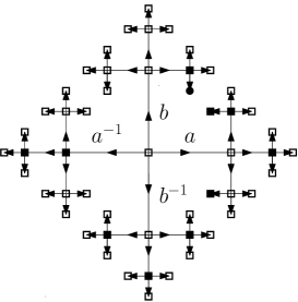
Figure 3: A Cayley graph of $\mathbb{F}_{2}$ and an element $(f,z)\in\mathbb{Z}_{2}\wr\mathbb{F}_{2}$. Black and white squares indicate that a value of $f$ at a given point is $c$ and $e$, respectively. The black disc indicates a position of the lamplighter $z$ and that $f(z)=c$.

In the first iteration consider a cyclic subgroup $A=\{a^{i}\,|\,i\in\mathbb{Z}\}\leqslant\mathbb{F}_{2}$ which forms a horizontal line in a Cayley graph of $\mathbb{F}_{2}$ with respect to $a$ and $b$, see Fig. 3. Scan this line from left to right checking for each $s\in A$ whether or not $V_{s}\neq\varnothing$, $f(s)=c$, $s=z$ and $s=e$. In case $V_{s}\neq\varnothing$, $s\neq e$ and $s\neq z$, write the symbols $D_{0}$ or $D_{1}$, if $f(s)=e$ or $f(s)=c$, respectively. Similarly, in case $V_{s}\neq\varnothing$, $s=e$ and $z\neq e$, write the symbols $D_{0}^{A}$ or $D_{1}^{A}$, in case $V_{s}\neq\varnothing$, $s=e$ and $z=e$, write the symbols $D_{0}^{B}$ or $D_{1}^{B}$ and in case $V_{s}\neq\varnothing$, $s=z$ and $s\neq e$, write the symbols $D_{0}^{C}$ or $D_{1}^{C}$, if $f(s)=e$ or $f(s)=c$, respectively. In case $V_{s}=\varnothing$, $s\neq e$ and $s\neq z$, write the symbols $0$ or $1$, if $f(s)=e$ or $f(s)=c$, respectively. Similarly, in case $V_{s}=\varnothing$, $s=e$ and $z\neq e$, write the symbols $A_{0}$ or $A_{1}$, in case $V_{s}=\varnothing$, $s=e$ and $z=e$, write the symbols $B_{0}$ or $B_{1}$ and in case $V_{s}=\varnothing$, $s=z$ and $s\neq e$, write the symbol $C_{0}$ or $C_{1}$, if $f(s)=e$ or $f(s)=c$, respectively. Finally, for the obtained bi–infinite string cut the infinite prefix and suffix consisting of $0$s, so the first and the last symbols of the remained finite string are not $0$. For the element of $\mathbb{Z}_{2}\wr\mathbb{F}_{2}$ shown in Fig. 3 the resulted string is $11D^{A}_{0}D_{0}1$.

In the second iteration each new $D$–symbol $\sigma$ is changed to a string of the form $(u^{-}\sigma u^{+})$, where the strings $u^{-}$ and $u^{+}$ are obtained as follows. Every $D$–symbol corresponds to a group element $s\in\mathbb{F}_{2}$. In order to construct $u^{-}$ scan the elements on a vertical ray $B_{s}^{-}=\{sb^{j}\,|\,j<0\}$ from bottom to top checking for each $t\in B_{s}^{-}$ whether or not $H_{t}\neq\varnothing$, $f(t)=c$ and $t=z$. In case $H_{t}\neq\varnothing$ and $t\neq z$, write the symbols $E_{0}$ or $E_{1}$, if $f(t)=e$ or $f(t)=c$, respectively. Similarly, in case $H_{t}\neq\varnothing$ and $t=z$, write the symbols $E_{0}^{C}$ or $E_{1}^{C}$, in case $H_{t}=\varnothing$ and $t\neq z$, write the symbols $0$ or $1$ and in case $H_{t}=\varnothing$ and $t=z$, write the symbols $C_{0}$ or $C_{1}$, if $f(t)=e$ or $f(t)=c$, respectively. Finally, for the obtained infinite string cut the infinite prefix of $0$s, so the first symbol of the remained finite string $u^{-}$ is not $0$. In a similar way a string $u^{+}$ is constructed by scanning the elements on a vertical ray $B_{s}^{+}=\{sb^{j}\,|\,j>0\}$ from bottom to top and cutting the infinite suffix consisting of $0$s. For the element shown in Fig. 3 the resulted string is $11(1E_{0}D_{0}^{A}E_{0})(E_{0}D_{0}E_{1})1$.

In the third iteration each new $E$–symbol $\mu$ is changed to a string of the form $[v^{-}\mu v^{+}]$, where the strings $v^{-}$ and $v^{+}$ are obtained as follows. Every $E$–symbol corresponds to a group element $t\in\mathbb{F}_{2}$. In order to construct $v^{-}$ scan the elements on a horizontal ray $A_{t}^{-}=\{ta^{i}\,|\,i<0\}$ from left to right checking for each $s\in A_{t}^{-}$ whether or not $V_{s}\neq\varnothing$, $f(s)=c$ and $s=z$. In case $V_{s}\neq\varnothing$ and $s\neq z$, write the symbols $D_{0}$ or $D_{1}$, if $f(s)=e$ or $f(s)=c$, respectively. Similarly, in case $V_{s}\neq\varnothing$ and $s=z$, write the symbols $E_{0}^{C}$ or $E_{1}^{C}$, if $f(s)=e$ or $f(s)=c$, respectively. In case $V_{s}=\varnothing$ and $s\neq z$, write the symbols $0$ or $1$, if $f(s)=e$ or $f(s)=c$, respectively. Similarly, in case $V_{s}=\varnothing$ and $s=z$, write the symbols $C_{0}$ or $C_{1}$, if $f(s)=e$ or $f(s)=c$, respectively. Finally, for the obtained infinite string cut the infinite prefix consisting of $0$s, so the first symbol of the remained finite string $v^{-}$ is not $0$. In a similar way a string $v^{+}$ is constructed by scanning the elements on a horizontal ray $A_{t}^{+}=\{ta^{i}\,|\,i>0\}$ from left to right and cutting the infinite suffix consisting of $0$s. For the element in Fig. 3 the resulted string is $11(1[1E_{0}1]D_{0}^{A}[E_{0}D_{1}])([1E_{0}]D_{0}[1E_{1}])1$.

This process is then repeated recursively until no new $D$ or $E$–symbols appear: for $i>1$ the $(2i)$th and the $(2i+1)$th iterations are performed exactly as the second and the third iterations described above, respectively. For the element in Fig. 3 the resulted string is $11(1[1E_{0}1]D_{0}^{A}[E_{0}(C_{1}D_{1})])([1E_{0}]D_{0}[1E_{1}])1$.

We remark that the symbols $C_{0},C_{1},D_{0}^{C},D_{1}^{C},E_{0}^{C},E_{1}^{C}$ and $A_{0},A_{1},D_{0}^{A},D_{1}^{A}$ are used to mark the position of the lamplighter $z\in\mathbb{F}_{2}$ and the identity $e\in\mathbb{F}_{2}$, respectively, when $z\neq e$. The symbols $B_{0},B_{1},D_{0}^{B},D_{1}^{B}$ are used to mark the position of the lamplighter and the identity when $z=e$.

For a given group element $g=(f,z)\in\mathbb{Z}_{2}\wr\mathbb{F}_{2}$, let $u\in\Sigma^{*}$ be a normal form of $g$ obtained by a recursive procedure described above. We denote by $L\subseteq\Sigma^{*}$ a language of all such normal forms. The described normal form of $\mathbb{Z}_{2}\wr\mathbb{F}_{2}$ defines a bijection $\psi:L\rightarrow\mathbb{Z}_{2}\wr\mathbb{F}_{2}$ mapping $u\in L$ to the corresponding group element $g\in\mathbb{Z}_{2}\wr\mathbb{F}_{2}$. This normal form is quasigeodesic [3, Theorem 5].

Construction of Turing machines computing the right multiplication in $\mathbb{Z}_{2}\wr\mathbb{F}_{2}$ by $a^{\pm 1},b^{\pm 1}$ and $c$. For the right multiplication in $\mathbb{Z}_{2}\wr\mathbb{F}_{2}$ by $c$, consider a one–tape Turing machine which reads the input $u\in\Sigma^{*}$ from left to right and when the head reads a symbol $D_{i}^{C}$, $E_{i}^{C}$, $D_{i}^{B}$, $C_{i}$ or $B_{i}$, $i=0,1$, it changes this symbol to $D_{j}^{C}$, $E_{j}^{C}$, $D_{j}^{B}$, $C_{j}$ or $B_{j}$, respectively, for $j=i+1\mod\,2$, and then it halts. If the head reads the blank symbol $\boxdot$, which indicates that the input $u$ has been read, it halts. This Turing machine halts in linear time for every input $u\in\Sigma^{*}$. Moreover, if the input $u\in L$, it computes the output $v\in L$ for which $\psi(u)c=\psi(v)$.

Let us describe a two–tape Turing machine computing the right multiplication by $a$ in $\mathbb{Z}_{2}\wr\mathbb{F}_{2}$ which halts in linear time on every input in $u\in\Sigma^{*}$. We refer to this Turing machine as $\mathrm{TM}_{a}$. We refer to the symbols $C_{0},C_{1},D_{0}^{C},D_{1}^{C},E_{0}^{C},E_{1}^{C}$ as $C$–symbols, $B_{0},B_{1},D_{0}^{B},D_{1}^{B}$ as $B$–symbols and $(,),[,]$ as brackets symbols.

Algorithm 8 (First iteration).

Initially for $\mathrm{TM}_{a}$ a content of the first tape is $\boxplus u\boxdot^{\infty}$ with a head over $\boxplus$. A content of the second tape is $\boxplus\boxdot^{\infty}$ with a head over $\boxplus$. In the first iteration $\mathrm{TM}_{a}$ moves a head associated to the first tape from left to right until it reads either $C$ or $B$–symbol. The second tape is used as a stack for storing the bracket symbols simultaneously checking their configuration:

• If a head on the first tape reads the symbol $($ or $[$, on the second tape a head moves right to the next cell and writes this symbol;

• If a head on the first tape reads the symbol $)$ or $]$, $\mathrm{TM}_{a}$ checks if a head on the second tape reads $($ or $[$, respectively. If not, $\mathrm{TM}_{a}$ halts. Otherwise, on the second tape a head writes the blank symbol $\boxdot$ and moves left to the previous cell.

If on the first tape a head does not read a $C$ or $B$–symbol, $\mathrm{TM}_{a}$ halts after a head reads a blank symbol $\boxdot$ indicating that the input has been read.

Let $S$ be the symbol a head associated to the first tape reads at the end of the first iteration. In the second iteration $\mathrm{TM}_{a}$ works depending on the symbol $S$. There are three cases to consider: $S\in\{D_{0}^{C},D_{1}^{C},D_{0}^{B},D_{1}^{B}\}$, $S\in\{E_{0}^{C},E_{1}^{C}\}$ and $S\in\{C_{0},C_{1},B_{0},B_{1}\}$.

Case 1. Suppose $S\in\{D_{0}^{C},D_{1}^{C},D_{0}^{B},D_{1}^{B}\}$. We notice that if the input $u\in L$ and $S\in\{D_{0}^{C},D_{1}^{C},D_{0}^{B},D_{1}^{B}\}$, then on the second tape a head must read the left bracket symbol $($. So if it is not the left bracket symbol $($, $\mathrm{TM}_{a}$ halts. If it is the left bracket symbol $($, $\mathrm{TM}_{a}$ continues working as described in Algorithm 9.

Algorithm 9 (Second iteration for Case 1).

First $\mathrm{TM}_{a}$ marks the left bracket symbol $($ on the second tape by changing it to $\mathring{(}$. On the first tape it changes the symbol $S$ to $D_{0}$, $D_{1}$, $D_{0}^{A}$ and $D_{1}^{A}$ if $S=D_{0}^{C}$, $D_{1}^{C}$, $D_{0}^{B}$ and $D_{1}^{B}$, respectively. Then $\mathrm{TM}_{a}$ proceeds as shown below.

1. $\mathrm{TM}_{a}$ keeps reading a content of the first tape while on the second tape it works exactly as in Algorithm 8 until on the first tape a head reads the right bracket symbol $)$ and, at the same time, on the second tape a head reads the marked left bracket symbol $\mathring{(}$. If such situation does not occur, $\mathrm{TM}_{a}$ halts after on the first tape a head reads a blank symbol $\boxdot$.

2. On the first tape a head moves right to the next cell and on the second tape a head writes the blank symbol $\boxdot$. Now let $S^{\prime}$ be the symbol that a head associated to the first tape reads. If $S^{\prime}\notin\{0,1,E_{0},E_{1},A_{0},A_{1},\boxdot,],(\,\}$, $\mathrm{TM}_{a}$ halts. Otherwise, depending on $S^{\prime}$, $\mathrm{TM}_{a}$ proceeds as follows.

   1. If $S^{\prime}=0,1,E_{0},E_{1},A_{0}$ or $A_{1}$, $\mathrm{TM}_{a}$ changes it to $C_{0}$, $C_{1}$, $E_{0}^{C}$, $E_{1}^{C}$, $B_{0}$ or $B_{1}$, respectively, and then halts.

   2. If $S^{\prime}=\boxdot$, $\mathrm{TM}_{a}$ changes it to $C_{0}$ and then halts.

   3. If $S^{\prime}=($, on the second tape a head writes the marked left bracket $\mathring{(}$ and on the first tape a head moves right to the next cell. After that $\mathrm{TM}_{a}$ keeps reading a content of the first tape while on the second tape it works exactly like in Algorithm 8 until a head associated to the first tape reads a symbol $Q=D_{0},D_{1},D_{0}^{A}$ or $D_{1}^{A}$ and, at the same time, a head associated to the second tape reads the marked left bracket $\mathring{(}$. If such situation does not occur, $\mathrm{TM}_{a}$ halts after on the first tape a head reads a blank symbol $\boxdot$. Finally $\mathrm{TM}_{a}$ changes the symbol $Q$ to $D_{0}^{C}$, $D_{1}^{C}$, $D_{0}^{B}$ or $D_{1}^{B}$, if $Q=D_{0},D_{1},D_{0}^{A}$ or $D_{1}^{A}$, respectively, and then it halts.

   4. If $S^{\prime}=\,]$, $\mathrm{TM}_{a}$ shifts a non–blank content of the first tape starting with this right bracket symbol $]$ by one position to the right and writes $C_{0}$ before it. Then $\mathrm{TM}_{a}$ halts.

Case 2. Suppose $S\in\{E_{0}^{C},E_{1}^{C}\}$. $\mathrm{TM}_{a}$ continues working as described in Algorithm 10.

Algorithm 10 (Second iteration for Case 2).

On the first tape $\mathrm{TM}_{a}$ changes $S$ to $E_{0}$ and $E_{1}$, if $S=E_{0}^{C}$ and $S=E_{1}^{C}$, respectively, and moves a head right to the next cell. Let $S^{\prime}$ be the symbol that a head associated to the first tape reads. If $S^{\prime}\notin\{0,1,(,]\}$, $\mathrm{TM}_{a}$ halts. Otherwise, depending on $S^{\prime}$, $\mathrm{TM}_{a}$ proceeds as shown below.

1. If $S^{\prime}=0$ or $1$, $\mathrm{TM}_{a}$ changes it to $C_{0}$ or $C_{1}$, respectively, and then halts.

2. If $S^{\prime}=($, on the second tape a head writes the marked left bracket $\mathring{(}$ and on the first tape a head moves right to the next cell. Then $\mathrm{TM}_{a}$ keeps reading a content of the first tape while on the second tape it works exactly as in Algorithm 8 until a head associated to the first tape reads a symbol $Q=D_{0}$ or $D_{1}$ and, at the same time, a head associated to the second tape reads the marked left bracket $\mathring{(}$. If such situation does not occur, $\mathrm{TM}_{a}$ halts after on the first tape a head reads a blank symbol $\boxdot$. Finally $\mathrm{TM}_{a}$ changes the symbol $Q$ to $D_{0}^{C}$ or $D_{1}^{C}$, if $Q=D_{0}$ or $D_{1}$, respectively, and halts.

3. If $S^{\prime}=\,]$, $\mathrm{TM}_{a}$ works exactly as in the case $d$ for the second stage of Algorithm 9.

Case 3. Suppose $S\in\{C_{0},C_{1},B_{0},B_{1}\}$. Let $P$ be the symbol a head associated to the second tape reads. We notice that if the input $u\in L$ and $S\in\{C_{0},C_{1}\}$, then $P\in\{(,[,\boxplus\}$. If $u\in L$ and $S\in\{B_{0},B_{1}\}$, then $P=\boxplus$. So if $S\in\{C_{0},C_{1}\}$ and $P\notin\{(,[,\boxplus\}$ or $S\in\{B_{0},B_{1}\}$ and $P\neq\boxplus$, $\mathrm{TM}_{a}$ halts. Otherwise, it continues working as described in Algorithm 11.

Algorithm 11 (Second iteration for Case 3).

Depending on $P$ and $S$, $\mathrm{TM}_{a}$ works as shown below.

1. If $P=($, then $\mathrm{TM}_{a}$ changes the symbol $S$ to the substring $w$ that is equal to $[E_{0}C_{0}]$ and $[E_{1}C_{0}]$, if $S=C_{0}$ and $S=C_{1}$, respectively. This can be done by shifting the non–blank content of the first tape following $S$ by three positions to the right and then wring $w$ before it; in particular, the symbol $S$ will be overwritten by the left bracket symbol $[$.

2. If $P=[$ and $S=C_{1}$, $\mathrm{TM}_{a}$ changes $C_{1}$ to $1$ and moves a head associated to the first tape by one position to the right. Let $S^{\prime}$ be the symbol a head associated to the first tape reads. If $S^{\prime}\notin\{0,1,E_{0},E_{1},(,]\}$, then $\mathrm{TM}_{a}$ halts. Otherwise, it continues working as shown below.

   • If $S^{\prime}\in\{0,1,E_{0},E_{1}\}$, then $\mathrm{TM}_{a}$ changes $S^{\prime}$ to $C_{0},C_{1},E_{0}^{C},E_{1}^{C}$ if $S^{\prime}=0,1,E_{0},E_{1}$, respectively, and then it halts.

   • If $S^{\prime}=($, then $\mathrm{TM}_{a}$ works exactly as in the case b for Algorithm 10.

   • If $S^{\prime}=\,]$, $\mathrm{TM}_{a}$ works exactly as in the case $d$ for the second stage of Algorithm 9.

3. If $P=[$ and $S=C_{0}$, $\mathrm{TM}_{a}$ moves a head associated to the first tape by one position to the left. Let $T$ be the symbol the head reads. Depending on $T$, $\mathrm{TM}_{a}$ proceeds as shown below.

   • If $T\neq[$, $\mathrm{TM}_{a}$ moves the head by one position to the right, changes $C_{0}$ to $0$ and moves the head again by one position to the right. After that, depending on the symbol $S^{\prime}$ the head reads, it continues working exactly as in the case b of the present algorithm.

   • If $T=[$, $\mathrm{TM}_{a}$ reads the two symbols following $C_{0}$. Let $S^{\prime}$ and $S^{\prime\prime}$ be the first and the seconds symbols following $C_{0}$, respectively. If $S^{\prime}\in\{E_{0},E_{1}\}$ and $S^{\prime\prime}=\,]$, then $\mathrm{TM}_{a}$ changes the substring $[C_{0}S^{\prime}]$ to the symbol $C_{0}$ or $C_{1}$ if $S^{\prime}=E_{0}$ or $S^{\prime}=E_{1}$, respectively. This can be done by shifting the non–blank content of the first tape following the substring $[C_{0}S^{\prime}]$ by three positions to the left and then changing the left bracket symbol $[$ to $C_{0}$ or $C_{1}$ if $S^{\prime}=E_{0}$ or $S^{\prime}=E_{1}$, respectively. If $S^{\prime}\notin\{E_{0},E_{1}\}$ or $S^{\prime\prime}\neq\,]$, $\mathrm{TM}_{a}$ shifts the non–blank content of the first tape following $C_{0}$ by one position to the left. Then, if $S^{\prime}\in\{0,1,E_{0},E_{1},(\}$, $\mathrm{TM}_{a}$ continues working exactly as in the case b of the present algorithm and halts otherwise.

4. If $P=\boxplus$, $\mathrm{TM}_{a}$ moves a head associated to the first tape by one position to the left. Let $T$ be the symbol the head reads. Depending on $S$ and $T$, $\mathrm{TM}_{a}$ proceeds as follows. If $T\neq\boxplus$ or $S\in\{C_{1},B_{0},B_{1}\}$, $\mathrm{TM}_{a}$ moves the head by one position to the right, changes $S$ to $0,1,A_{0}$ or $A_{1}$, if $S=C_{0},C_{1},B_{0}$ or $B_{1}$, respectively, and moves the head again by one position to the right. If $T=\boxplus$ and $S=C_{0}$, $\mathrm{TM}_{a}$ shifts the non–blank content of the first tape following $C_{0}$ by one position to the left erasing $C_{0}$ and places the head over the first symbol after $\boxplus$. Now let $S^{\prime}$ be a symbol the head reads. If $S^{\prime}\notin\{0,1,A_{0},A_{1},\boxdot,(\}$, $\mathrm{TM}_{a}$ halts. Otherwise, if $S^{\prime}\in\{0,1,A_{0},A_{1},\boxdot\}$, $\mathrm{TM}_{a}$ changes $S^{\prime}$ to $C_{0},C_{1},B_{0},B_{1}$ and $C_{0}$ if $S^{\prime}=0,1,A_{0},A_{1}$ and $\boxdot$, respectively, and then halts. If $S^{\prime}=($, $\mathrm{TM}_{a}$ moves a head associated to the second tape by one position to the right. After that it continues working exactly as in the case c for the stage 2 of Algorithm 9.

The runtime of Algorithm 8 is linear. Also, as shifting a portion of a tape by a fixed number of positions requires at most linear time, for each of the algorithms 9–11 the runtime is linear. Therefore, $\mathrm{TM}_{a}$ halts in linear time for every input $u\in\Sigma^{*}$. Moreover, if the input $u\in L$, $\mathrm{TM}_{a}$ halts with the output $v\in L$ for which $\psi(u)a=\psi(v)$ written on the first tape. Two–tape Turing machines computing the right multiplication by $a^{-1}$ and $b^{\pm 1}$ which halt in linear time one every input are constructed in the same way as $\mathrm{TM}_{a}$ with minor modifications. Thus we have the following theorem.

Theorem 12.

The wreath product $\mathbb{Z}_{2}\wr\mathbb{F}_{2}$ is Cayley $2$–tape linear–time computable.

5 Thompson’s Group $F$

In this section we show that Richard Thompson’s group $F$ is Cayley $2$–tape linear–time computable. The group $F=\langle x_{0},x_{1}\,|\,[x_{0}^{-1}x_{1},x_{0}^{-1}x_{1}x_{0}],[x_{0}^{-1}x_{1},x_{0}^{-2}x_{1}x_{0}^{2}]\rangle$ admits the infinite presentation of the form:

$$F=\langle x_{0},x_{1},x_{2}\dots\,|\,\,x_{j}x_{i}=x_{i}x_{j+1}\,\,\mathrm{for}\,\,i<j\rangle.$$

This infinite presentation provides a standard infinite normal form for elements of $F$ with respect to generators $x_{i}$, $i\geqslant 0$, discussed by Brown and Geoghegan [16]. Namely, applying the relations $x_{j}x_{i}=x_{i}x_{j+1}$ for $i<j$, a group element $g\in F$ can be written uniquely as:

$$x_{i_{0}}^{e_{0}}x_{i_{1}}^{e_{1}}\dots x_{i_{m}}^{e_{m}}x_{j_{n}}^{-f_{n}}\dots x_{j_{1}}^{-f_{1}}x_{j_{0}}^{-f_{0}},$$ (1)

where

• $0\leqslant i_{0}<i_{1}<i_{2}<\dots<i_{m}$ and $0\leqslant j_{0}<j_{1}<j_{2}<\dots<j_{n}$;

• $e_{i},f_{j}>0$ for all $i,j$;

• if $x_{i}$ and $x_{i}^{-1}$ are both present in the expression, then so is $x_{i+1}$ or $x_{i+1}^{-1}$.

For other equivalent interpretations of Thompson’s group $F$, as the set of piecewise linear homomorphisms of the interval $[0,1]$ and as the set of pairs of reduced finite rooted binary trees, we refer the reader to [6].

Normal form. Based on the standard infinite normal form (1) Elder and Taback [9] constructed a normal form for elements of $F$ over the alphabet $\Sigma=\{a,b,\#\}$ as follows. Let $M=\max\{i_{m},j_{n}\}$. First let us rewrite (1) in the form such that every generator $x_{i},i=0,\dots,M$ appears twice:

$$x_{0}^{r_{0}}x_{1}^{r_{1}}x_{2}^{r_{2}}\dots x_{M}^{r_{M}}x_{M}^{-s_{M}}\dots x_{2}^{-s_{2}}x_{1}^{-s_{1}}x_{0}^{-s_{0}},$$ (2)

where $r_{i},s_{i}\geqslant 0$, exactly one of $r_{M},s_{M}$ is nonzero, and $r_{i}s_{i}>0$ implies $r_{i+1}+s_{i+1}>0$. After that we rewrite (2) in the following form:

$$a^{r_{0}}b^{s_{0}}\#a^{r_{1}}b^{s_{1}}\#\dots\#a^{r_{M}}b^{s_{M}},$$ (3)

where again $r_{i},s_{i}\geqslant 0$, exactly one of $r_{M},s_{M}$ is nonzero, and $r_{i}s_{i}>0$ implies $r_{i+1}+s_{i+1}>0$. We denote by $L_{\infty}$ the language of all strings of the form (3). The language $L_{\infty}$ is regular [9, Lemma 3.1]. Following the notation in [9], for a given $u=a^{r_{0}}b^{s_{0}}\#a^{r_{1}}b^{s_{1}}\#\dots\#a^{r_{M}}b^{s_{M}}$ from the language $L_{\infty}$ we denote by $\overline{u}$ the corresponding group element $x_{0}^{r_{0}}x_{1}^{r_{1}}x_{2}^{r_{2}}\dots x_{M}^{r_{M}}x_{M}^{-s_{M}}\dots$ $x_{2}^{-s_{2}}x_{1}^{-s_{1}}x_{0}^{-s_{0}}$ in $F$. The described normal form of $F$ defines a bijection between $L_{\infty}$ and $F$ mapping $u$ to $\overline{u}$. This normal form is quasigeodesic [9, Proposition 3.3]

Construction of Turing machines computing the right multiplication in $F$ by $x_{0}^{\pm 1}$ and $x_{1}^{\pm 1}$. By [9, Proposition 3.4] the language $L_{x_{0}^{-1}}=\{\otimes(u,v)\,|\,u,v\in L_{\infty},\overline{u}x_{0}^{-1}=_{F}\overline{v}\}$ is regular. This implies that there is a linear–time algorithm that from a given input $u\in L_{\infty}$ computes the output $v\in L_{\infty}$ such that $\overline{u}x_{0}^{-1}=_{F}\overline{v}$; see, e.g., [10, Theorem 2.3.10]. Moreover, this algorithm can be done in linear time on a one–tape Turing machine [7, Theorem 2.4]. Thus we only have to analyze the right multiplication by $x_{1}^{\pm 1}$. Below we will show that the right multiplication in the group $F$ by $x_{1}^{\pm 1}$ can be computed in linear time on a $2$–tape Turing machine.

We denote by $w$ the infinite normal form (1) for a group element $g\in F$. We denote by $u$ and $v$ the normal forms (3) for $g$ and $gx_{1}^{-1}$, respectively; that is, $\overline{u}=g$ and $\overline{v}=gx_{1}^{-1}$. Let us describe multi–tape Turing machines computing the right multiplication by $x_{1}^{-1}$ and $x_{1}$ in $F$ which halts in linear time on every input in $\Sigma^{*}$. We refer to these Turing machines as $\mathrm{TM}_{x_{1}^{-1}}$ and $\mathrm{TM}_{x_{1}}$, respectively. Initially for $\mathrm{TM}_{x_{1}^{-1}}$ a content of the first tape is $\boxplus u\boxdot^{\infty}$ with the head over $\boxplus$. For $\mathrm{TM}_{x_{1}}$ a content of the first tape is $\boxplus v\boxdot^{\infty}$ with the head over $\boxplus$. A content for each of the other tapes is $\boxplus\boxdot^{\infty}$ with the head over $\boxplus$. We may assume that the input is in the regular language of normal forms $L_{\infty}$. This can be verified in linear time by reading the input on the first tape. If the input is not in $L_{\infty}$, a Turing machine halts. Otherwise, a head associated to the first tape returns to its initial position over the $\boxplus$ symbol.

The general descriptions of $\mathrm{TM}_{x_{1}^{-1}}$ and $\mathrm{TM}_{x_{1}}$ are as follows. For the input $u$ a Turing machine $\mathrm{TM}_{x_{1}^{-1}}$ verifies each of the cases described by Elder and Taback in [9, Proposition 3.5] one by one. Once it finds a valid case, it runs a subroutine computing $v$ from $u$ and writes it on the first tape. Then $\mathrm{TM}_{x_{1}^{-1}}$ halts. For the input $v$ a Turing machine $\mathrm{TM}_{x_{1}}$ first copies it on the second tape where it is stored until it halts. Then $\mathrm{TM}_{x_{1}}$ tries each of the cases one by one. For the case being tried it runs a subroutine computing $u$ from $v$ written on the second tape and writes the output $u$ on the first tape. Then it verifies whether or not the case being tried is valid for $u$. If it is valid, then it runs the corresponding subroutine for $\mathrm{TM}_{x_{1}^{-1}}$ computing $v$ from $u$ and writes it on a third tape; otherwise, it tries the next case. Then $\mathrm{TM}_{x_{1}^{-1}}$ verifies whether or not the contents of the second and the third tapes are the same. If they are the same, then $\mathrm{TM}_{x_{1}^{-1}}$ halts; otherwise, $\mathrm{TM}_{x_{1}^{-1}}$ tries the next case. As there are only finitely many cases to try, $\mathrm{TM}_{x_{1}^{-1}}$ will halt with the string $u$ written on the first tape. For each of the cases in [9, Proposition 3.5] we describe a subroutine for its validity verification, a subroutine for computing $v$ from $u$ and a subroutine for computing $u$ from $v$.

Case 1: Suppose that $s_{0}=0$ or, equivalently, the infinite normal form $w$ does not contain $x_{0}$ to a negative exponent. That is, $u$ is either of the form $u=a^{r_{0}}\#\gamma$ for $\gamma\in\Sigma^{*}$ or $u=a^{r_{0}}$, where $r_{0}\geqslant 0$. This case can be verified by reading $u$. There are the following three cases to consider.

Case 1.1: The normal form $u$ is of the form $u=a^{r_{0}}$ for $r_{0}\geqslant 0$. This case can be verified by reading $u$. If $u=a^{r_{0}}$ for $r_{0}\geqslant 0$, then $v=a^{r_{0}}\#b$. A subroutine for computing $v$ from $u$ appends the suffix $\#b$ to $u$. A subroutine for computing $u$ from $v$ erases the last two symbols of $v$ by writing the blank symbols $\boxdot\boxdot$.

Case 1.2: The normal from $u$ contains at least one $\#$ symbol and $wx_{1}^{-1}$ is the infinite normal form for $gx_{1}^{-1}$. The latter is true if at least one of the following conditions holds.

1. The expression $w$ contains no $x_{1}$ terms to a positive exponent: $r_{1}=0$;

2. The expression $w$ contains $x_{1}$ to a negative power: $s_{1}\neq 0$;

3. The expression $w$ contains $x_{2}$ to a nonzero power: $r_{2}\neq 0$ or $s_{2}\neq 0$.

Each of these three conditions can be verified by reading $u$. If $u=a^{r_{0}}\#a^{r_{1}}b^{s_{1}}\gamma$, where $\gamma$ is empty or begins with $\#$, then $v=a^{r_{0}}\#a^{r_{1}}b^{s_{1}+1}\gamma$. A subroutine for computing $v$ from $u$ shifts a suffix $b^{s_{1}}\gamma$ by one position to the right and writes the $b$ symbol before it. A subroutine for computing $u$ from $v$ shifts the suffix $b^{s_{1}}\gamma$ by one position to the left.

Case 1.3: The normal form $u$ is of the form $u=a^{r_{0}}\#a^{r_{1}}\gamma$ with $r_{1}>0$ and $\gamma$ is either empty or $\gamma=\#\#\gamma^{\prime}$ for $\gamma^{\prime}\in\Sigma^{*}$. This case can be trivially verified by reading $u$. The infinite normal form $w$ is $w=x_{0}^{r_{0}}x_{1}^{r_{1}}\eta$, where $\eta$ is either empty or $\eta=x_{i}^{r_{i}}\dots x_{j}^{-s_{j}}$ for some $i,j>2$. Then $wx_{1}^{-1}=x_{0}^{r_{0}}x_{1}^{r_{1}}\eta x_{1}^{-1}=x_{0}^{r_{0}}x_{1}^{r_{1}}\eta^{\prime}$, where $\eta^{\prime}$ is obtained from $\eta$ replacing $x_{i}^{\pm 1}$ by $x_{i-1}^{\pm 1}$. Therefore, for $u=a^{r_{0}}\#a^{r_{1}}\gamma$ we have the following three subcases.

1. If $r_{1}>1$ and $\gamma$ is empty, then $v=a^{r_{0}}\#a^{r_{1}-1}$. A subroutine for computing $v$ from $u$ erases the last symbol of $u$ by writing the blank symbol $\boxdot$. A subroutine for computing $u$ from $v$ appends the $a$ symbol to $v$.

2. If $r_{1}=1$ and $\gamma$ is empty, then $v=a^{r_{0}}$. A subroutine for computing $v$ from $u$ erases the last two symbols of $u$ by writing $\boxdot\boxdot$. A subroutine for computing $u$ from $v$ appends $\#a$ to $v$.

3. If $r_{1}>1$ and $\gamma=\#\#\gamma^{\prime}$, then $v=a^{r_{0}}\#a^{r_{1}-1}\#\gamma^{\prime}$. A subroutine for computing $v$ from $u$ shifts the suffix $\#\gamma^{\prime}$ by two positions to the left. A subroutine for computing $u$ from $v$ shifts the suffix $\#\gamma^{\prime}$ by two positions to the right and writes $a\#$ before it.

All described subroutines for Cases 1 can be done in linear time on one tape.

Case 2: Suppose that $s_{0}\neq 0$. That is, $u$ is either of the form $u=a^{r_{0}}b^{s_{0}}\#\gamma$ for $\gamma\in\Sigma^{*}$ or $u=a^{r_{0}}b^{s_{0}}$, where $r_{0}\geqslant 0$ and $s_{0}>0$. This can be verified in linear time by reading $u$. Since $w$ ends in $x_{0}^{-1}$, $wx_{1}^{-1}$ is not the infinite normal form for $gx_{1}^{-1}$. Applying the relations $x_{0}^{-1}x_{j}^{-1}=x_{j+1}^{-1}x_{0}^{-1}$, $j>0$, $f_{0}$ times we obtain that if $1+f_{0}\leqslant j_{1}$, $gx_{1}^{-1}$ is equal to $x_{i_{0}}^{e_{0}}x_{i_{1}}^{e_{1}}\dots x_{i_{m}}^{e_{m}}x_{j_{n}}^{-f_{n}}\dots x_{j_{1}}^{-f_{1}}x_{1+f_{0}}^{-1}x_{0}^{-f_{0}}$. If $1+f_{0}>j_{1}$, then applying the relations $x_{j_{1}}^{-1}x_{j}^{-1}=x_{j+1}^{-1}x_{j_{1}}^{-1}$, $j>j_{1}$, $f_{1}$ times we obtain that if $1+f_{0}+f_{1}\leqslant j_{2}$, $gx_{1}^{-1}$ is equal to $x_{i_{0}}^{e_{0}}x_{i_{1}}^{e_{1}}\dots x_{i_{m}}^{e_{m}}x_{j_{n}}^{-f_{n}}\dots x_{j_{2}}^{-f_{2}}x_{1+f_{0}+f_{1}}^{-1}x_{j_{1}}^{-f_{1}}x_{0}^{-f_{0}}$. This process is continued until the first time we obtain $x_{R}^{-1}$ where either:

• $R=1+f_{0}+f_{1}+\dots+f_{n}>j_{n}$, or

• $R=1+f_{0}+f_{1}+\dots+f_{t}\leqslant j_{t+1}$ for some $0\leqslant t\leqslant n-1$.

In Algorithm 13 below we describe a two–tape Turing machine $\mathrm{TM}_{R}$ that for a given normal form $u$ written on the first tape writes a string $b^{R}$ on the second tape.

Algorithm 13 (A subroutine for computing $R$).

Initially a content of the first tape is $\boxplus u\boxdot^{\infty}$ with a head over $\boxplus$. A content of the second tape is $\boxplus\boxdot^{\infty}$ with a head over $\boxplus$. Let  $\mathrm{STOP}_{1}$ be a boolean variable which is true if a head on the first tape reads $\boxdot$ and false otherwise, let  $\mathrm{STOP}_{2}$ be a boolean variable which is true if a head on the second tape reads $\boxplus$ and false otherwise. Finally let $\mathrm{CASE}$ be a boolean variable which is true if $R>j_{n}$ and false if $R=1+f_{0}+\dots+f_{t}\leqslant j_{t+1}$ for some $0\leqslant t\leqslant n-1$.

1. On the first tape $\mathrm{TM}_{R}$ moves a head by one position to the right. On the second tape $\mathrm{TM}_{R}$ moves a head by one position to the right and writes the symbol $b$.

2. While $\mathrm{not}$ $(\mathrm{STOP_{1}}$ $\mathrm{or}$ $\mathrm{STOP_{2}})$:

   1. If a head on the first tape reads the $a$ symbol, on the first tape $\mathrm{TM}_{R}$ moves the head by one position to the right.

   2. If a head on the first tape reads the $b$ symbol, on the second tape $\mathrm{TM}_{R}$ moves the head by one position to the right and writes the $b$ symbol while on the first tape it moves a head by one position to the right.

   3. If a head on the first tape reads the $\#$ symbol, on the second tape $\mathrm{TM}_{R}$ writes the blank symbol $\boxdot$ and moves a head by one position to the left while on the first tape it moves a head by one position to the right.

3. To find a correct value of the boolean variable $\mathrm{CASE}$ the subroutine proceeds as follows.

   1. If  $\mathrm{STOP_{1}}$, we set $\mathrm{CASE=true}$.

   2. If  $\mathrm{not}$ $\mathrm{STOP_{1}}$, on the first tape $\mathrm{TM}_{R}$ checks if a head reads the $b$ symbol. If not, on the first tape it moves a head by one position to the right and checks again if a head reads the $b$ symbol. This process is continued until either a head reads $\boxdot$ or the $b$ symbol. If it reads $\boxdot$, we set $\mathrm{CASE=true}$. If it reads the $b$ symbol, we set $\mathrm{CASE=false}$.

4. Then $\mathrm{TM}_{R}$ erases all $b$ symbols on the second tape. If a head on the second tape reads the $b$ symbol it writes $\boxdot$ and moves a head by one position to the left. This process is continued until a head on the second tape reads $\boxplus$.

5. Depending on the value of $\mathrm{CASE}$ the subroutine proceeds as follows.

   1. Suppose $\mathrm{CASE}$. First a head on the second tape moves by one position to the right and writes the $b$ symbol. Then, if a head on the first tape reads the $b$ symbol, it moves by one position to the left while a head on the second tape moves by one position to the right and writes the $b$ symbol. If a head on the first tape reads $\#$ or the $a$ symbol, it moves by one position to the left. This process is continued until a head on the first tape reads $\boxplus$.

   2. Suppose $\mathrm{not}$ $\mathrm{CASE}$. If a head on the first tape reads the $b$ symbol, it moves by one position to the left while a head on the second tape moves by one position to the right and writes the $b$ symbol. If a head on the first tape reads $\#$ or the $a$ symbol, it moves by one position to the left. This process is continued until a head on the first tape reads $\boxplus$.

From Algorithm 13 it can be seen that a subroutine for computing $R$ can be done in linear time on a two–tape Turing machine. Depending on the value of $\mathrm{CASE}$ we consider the following two cases.

Case 2.1: Suppose $\mathrm{CASE}$. That is, $R>j_{n}$. Let $M=\max\{i_{m},j_{n}\}$. There are three subcases to consider: $R>M$, $R=M$ and $R<M$. Each of these three subcases can be checked as follows. First note that $M$ is just the number of $\#$ symbols in the normal form $u$. So we run a subroutine which reads $u$ on the first tape and each time a head reads the $\#$ symbol, on a separate tape it moves a head by one position to the right and writes the $\#$ symbol. In the end of this subroutine the content of this separate tape is $\boxplus\#^{M}\boxdot^{\infty}$. Now to check whether $R>M$, $R=M$ or $R<M$ we can synchronously read the tapes $\boxplus b^{R}\boxdot^{\infty}$ and $\boxplus\#^{M}\boxdot^{\infty}$ with the heads initially over the $\boxplus$ symbols.

(a) Suppose $R>M$. Then the infinite normal form of $gx_{1}^{-1}$ is

$$x_{i_{0}}^{e_{0}}x_{i_{1}}^{m_{1}}\dots x_{i_{m}}^{e_{m}}x_{R}^{-1}x_{j_{n}}^{-f_{n}}\dots x_{j_{2}}^{-f_{2}}x_{j_{1}}^{-f_{1}}x_{0}^{-f_{0}},$$

where $f_{0}\neq 0$. We write $u$ in the form $u=a^{r_{0}}b^{s_{0}}\gamma$, where $\gamma$ is either empty or starts with $\#$, ends with $a$ or $b$ and contains exactly $M$ $\#$ symbols. Then $v=a^{r_{0}}b^{s_{0}}\gamma\#^{R-M}b$. A subroutine for computing $v$ from $u$ appends the string $\#^{R-M}b$ to $u$ as follows. First a head on the first tape where $u$ is written moves to the last non–blank symbol. Then we synchronously read the tapes $\boxplus b^{R}\boxdot^{\infty}$ and $\boxplus\#^{M}\boxdot^{\infty}$ from the beginning until both heads are over the $\boxdot$ symbols. If a head on the tape $\boxplus b^{R}\boxdot^{\infty}$ reads the $b$ symbol but a head on the tape $\boxplus\#^{M}\boxdot^{\infty}$ reads $\boxdot$, on the first tape a head moves by one position to the right and writes the $\#$ symbol. As a result the content of a first tape will be $\boxplus a^{r_{0}}b^{r_{0}}\gamma\#^{R-M}\boxdot^{\infty}$ with a head over the last $\#$ symbol. After that a head on the first tape moves by one position to right and writes the $b$ symbol.

A subroutine for computing $u$ from $v$ moves a head to the last symbol of $u$, which is $b$. Then it writes the $\boxdot$ and moves a head by one position to the left. If a head reads $\#$ it writes $\boxdot$ and moves a head by one position to the left. This process is continued until a head reads a symbol which is not $\#$. As a result the content of a first tape will be $\boxplus a^{r_{0}}b^{s_{0}}\gamma\boxdot^{\infty}$.

(b) Suppose $R=M$. This can only occur if $R=i_{m}$. Then the infinite normal form of $gx_{1}^{-1}$ is either:

$$x_{i_{0}}^{e_{0}}x_{i_{1}}^{e_{1}}\dots x_{i_{m}}^{e_{m}-1}x_{j_{n}}^{-f_{n}}\dots x_{j_{2}}^{-f_{2}}x_{j_{1}}^{-f_{1}}x_{j_{0}}^{-f_{0}}\,\,\mathrm{if}\,\,e_{m}>1,\mathrm{or}$$

$$x_{i_{0}}^{e_{0}}x_{i_{1}}^{e_{1}}\dots x_{i_{m-1}}^{e_{m-1}}x_{j_{n}}^{-f_{n}}\dots x_{j_{2}}^{-f_{2}}x_{j_{1}}^{-f_{1}}x_{j_{0}}^{-f_{0}}\,\,\mathrm{if}\,\,e_{m}=1.$$

The latter expression is an infinite normal form as $i_{m}=R\geqslant j_{n}+2$ and $w$ is an infinite normal form. Indeed, for Case 2.1 we have that $1+f_{0}+\dots+f_{n-1}>j_{n}$. Therefore,

$$R=1+f_{0}+\dots+f_{n-1}+f_{n}\geqslant j_{n}+2.$$ (4)

If we write $u$ in the form $u=\gamma\#^{s}a^{e_{m}}$, then $v=\gamma\#^{s}a^{e_{m}-1}$ when $e_{m}>1$ and $v=\gamma$ if $e_{m}=1$.

A subroutine for computing $v$ from $u$ reads $u$ to check if $e_{m}>1$ or $e_{m}=1$. If $e_{m}>1$, it erases the last $a$ symbol by writing $\boxdot$. If $e_{m}=1$, it erases the last $a$ symbol by writing $\boxdot$ and moves a head by one position to the left. If a head reads $\#$ it writes $\boxdot$ and moves by one position to the left. This is continued until a head reads a symbol which is not $\#$. As a result the content of the first tape will be $\boxplus\gamma\boxdot^{\infty}$.

A subroutine for computing $u$ from $v$ is a follows. First we run Algorithm 13 for the input $v$. As result we get $\boxplus b^{R}\boxdot^{\infty}$ written on a second tape. Now let $M^{\prime}$ be the number of $\#$ symbols in $v$. Like in the subcase (a) of Case 2.1 we run a subroutine that computes $M^{\prime}$ and appends $\#^{R-M^{\prime}}$ to $v$ if $R\geqslant M^{\prime}$; if $R<M^{\prime}$ the consideration of this subcase (b) is skipped. Finally in the last step it appends $a$. As a result the content of the first tape will be $\boxplus\gamma\#^{R-M^{\prime}}a\boxdot^{\infty}$ if $R>M^{\prime}$ and $\boxplus\gamma a\boxdot^{\infty}$ if $R=M^{\prime}$.

(c) Suppose $R<M$. Then $i_{m}=M$. There are three subsubcases to consider.

1) The generator $x_{R}$ does not appear in $w$. That is, $u$ is of the form $u=\gamma\#a^{r_{R-1}}\#\#\eta$, where $\eta\in\{a,\#\}^{*}$; note that $s_{R-1}=0$ by the inequality (4). This subsubcase is verified by finding the $R$th $\#$ symbol in $u$ and checking whether or not the next symbol after it is $a$. If it is not $a$, then $x_{R}$ does not appear in $w$. If we write $u$ in the form $u=\gamma\#a^{r_{R-1}}\#\#\eta$, then $v=\gamma\#a^{r_{R-1}}\#b\#\eta$. A subroutine for computing $v$ from $u$ inserts the $b$ symbol before the $(R+1)$th $\#$ symbol – it shifts the suffix $\#\eta$, which begins with the $(R+1)$th $\#$ symbol, by one position to the right and writes the $b$ symbol before it. A subroutine for computing $u$ from $v$ shifts the suffix $\#\eta$ by one position to the left erasing the $b$ symbol. This can be done without knowing $b^{R}$ written on another tape: we read $v$ from the right to the left until a head reads the $b$ symbol, then we shift the suffix $\#\eta$ following it by one position to the left. This is a correct algorithm as the suffix $\eta$ does not have any $b$ symbols.

2) The generator $x_{R}$ appears in $w$ together with $x_{R+1}$. That is, $u$ is either of the form $u=\gamma\#a^{r_{R}}\#a^{r_{R+1}}\eta$, with $r_{R},r_{R+1}>0$ , where $\eta\in\{a,\#\}^{*}$ is either empty or begins with $\#$. This subsubcase is verified by finding the $R$th and $(R+1)$th $\#$ symbols in $u$ and checking whether or not both symbols after them are $a$. If both of them are $a$, then $x_{R}$ and $x_{R+1}$ appear in $w$. If we write $u$ in the form $u=\gamma\#a^{r_{R}}\#a^{r_{R+1}}\eta$, then $v=\gamma\#a^{r_{R}}b\#a^{r_{R+1}}\eta$. A subroutine for computing $v$ from $u$ inserts the $b$ symbol before the $(R+1)$th $\#$ symbol like in the previous subsubcase. A subroutine for computing $u$ from $v$ shifts the suffix $\#a^{r_{R+1}}\eta$ by one position to the left erasing the $b$ symbol. Like in the previous case this can be done without knowing $b^{R}$ written on another tape: we read $v$ from the right to the left until a head reads the $b$ symbol, then we shift the suffix following it by one position to the left.

3) The generator $x_{R}$ appears in $w$ but $x_{R+1}$ does not appear in $w$. That is, $u$ is of the form $u=\gamma\#a^{r_{R}}\#\#\eta$, where $\eta\in\{a,\#\}^{*}$. This subsubcase is verified by checking whether or not the first symbol after the $R$th $\#$ symbol is $a$ and the first symbol after the $(R+1)$th $\#$ symbol is not $a$. If the latter is true, then $x_{R}$ appears in $w$ but $x_{R+1}$ does not. Now if $u=\gamma\#a^{r_{R}}\#\#\eta$, where $\eta\in\{a,\#\}^{*}$, then $v=\gamma\#a^{r_{R}-1}\#\eta$; note that for $r_{R}=1$, $v$ is a valid normal form by the inequality (4). A subroutine for computing $v$ from $u$ shifts the suffix $\#\eta$ following the $(R+1)$th $\#$ symbol by two positions to the left erasing the subword $a\#$ that precedes this suffix. A subroutine for computing $u$ from $v$ first runs Algorithm 13 for the input $v$ writing $\boxplus b^{R}\boxdot^{\infty}$ on a second tape and then inserts the subword $a\#$ before the suffix $\#\eta$ which begins with the $(R+1)$th $\#$ symbol; if the $(R+1)$th $\#$ symbol is not found in $v$ then the consideration of this subsubcase is skipped.

Case 2.2: Suppose $\mathrm{not}$ $\mathrm{CASE}$. That is, $R=1+f_{0}+f_{1}+\dots+f_{t}\leqslant j_{t+1}$ for some $0\leqslant t\leqslant n-1$. Then $gx_{1}^{-1}$ is equal to:

$$x_{i_{0}}^{e_{0}}x_{i_{1}}^{e_{1}}\dots x_{i_{m}}^{e_{m}}x_{j_{n}}^{-f_{n}}\dots x_{j_{t+1}}^{-f_{t+1}}x_{R}^{-1}x_{j_{t}}^{-f_{t}}\dots x_{j_{0}}^{-f_{0}}.$$ (5)

Note that $R>j_{t}$ by the construction of $R$. There are two cases to consider depending whether or not (5) is an infinite normal form.

Case 2.2.1: Suppose that (5) is not an infinite normal form. This only happens when $R<j_{t+1}$ and for $w$ the generator $x_{R}$ is present to a positive power while $x_{R+1}$ is not present to any non–zero power. This situation occurs only if there is an index $p\leqslant m$ for which $i_{p}=R$, $i_{p+1}\neq R+1$ and $j_{t+1}\neq R+1$. That is, $u$ is of the form $u=\gamma\#a^{r_{R}}\#\#\eta$. This subcase is verified by finding the $(R+1)$th $\#$ symbol and checking if the previous symbol is $a$ and the next symbol is $\#$. If we write $u$ in the form $u=\gamma\#a^{r_{R}}\#\#\eta$, then $v=\gamma\#a^{r_{R}-1}\#\eta$. Note that for $r_{R}=1$, $v$ is a valid normal form since $R>j_{t}+1$; this is because $1+f_{0}+\dots+{f_{t-1}}>j_{t}$, so $R=1+f_{0}+\dots+f_{t-1}+f_{t}>j_{t}+1$.

A subroutine for computing $v$ from $u$ shifts the suffix $\#\eta$ following the $(R+1)$th $\#$ symbol by two positions to the left erasing the subword $a\#$ that precedes this suffix. A subroutine for computing $u$ from $v$ is the same as for the subsubcase (c).3 of Case 2.1: it runs Algorithm 13 for the input $v$ and then inserts the subword $a\#$ before the suffix $\#\eta$ which begins with the $(R+1)$th $\#$ symbol. Note that for Case 2.2.1 $R$ must be the same for $u$ and $v$ as $R<j_{t+1}$.

Case 2.2.2: Suppose that (5) is an infinite normal form. This happens only in the following subcases.

1. $x_{R}^{-1}$ is already in $w$, that is, $R=j_{t+1}$. That is, $u$ is of the form $u=\gamma\#a^{r_{R}}b^{s_{R}}\eta$ with $s_{R}>0$, where $\eta$ is either empty or begins with $\#$. This subcase is verified by finding the $R$th $\#$ symbol in $u$ and checking if the suffix following it is of the form $a^{k}b\mu$ for $k\geqslant 0$. If we write $u$ in the form $u=\gamma\#a^{r_{R}}b^{s_{R}}\eta$, then $v=\gamma\#a^{r_{R}}b^{s_{R}+1}\eta$. A subroutine for computing $v$ from $u$ first reads the input $u$ until it finds the $R$th $\#$ symbol. Then it reads the suffix $a^{r_{R}}b^{s_{R}}\eta$ until it reads the $b$ symbol first time. After that it shifts the suffix $b^{s_{R}}\eta$ by one position to the right and writes the $b$ symbol before it. A subroutine for computing $u$ from $v$ first reads the input $v$ until it finds the $R$th $\#$ symbol. Then it reads the suffix $a^{r_{R}}b^{s_{R}+1}\eta$ until it reads the $b$ symbol first time. After that it erases this $b$ symbol and shifts the suffix following it by one position to the left.

2. $x_{R}^{-1}$ is not in $w$, but $x_{R}$ and either $x_{R+1}$ or $x_{R+1}^{-1}$ are present in $w$. That is, $u$ is of the form $u=\gamma\#a^{r_{R}}\#a^{r_{R+1}}b^{s_{R+1}}\eta$ with $r_{R}>0$ and $r_{R+1}+s_{R+1}>0$, where $\eta$ is either empty of begins with $\#$. This subcase is verified by finding the the $R$th $\#$ symbol in $u$ and checking if the suffix following it is of the form $a^{k}\#a\mu$ or $a^{k}\#b\mu$ for $k\geqslant 1$. If we write $u$ in the form $u=\gamma\#a^{r_{R}}\#a^{r_{R+1}}b^{s_{R+1}}\eta$, then $v=\gamma\#a^{r_{R}}b\#a^{r_{R+1}}b^{s_{R+1}}\eta$. A subroutine for computing $v$ from $u$ inserts the $b$ symbol before the suffix $\#a^{r_{R+1}}b^{s_{R+1}}\eta$ which begins with the $(R+1)$th $\#$ symbol. A subroutine for computing $u$ from $v$ shifts the suffix $\#a^{r_{R+1}}b^{s_{R+1}}\eta$ by one position to the left which erases the $b$ symbol preceding this suffix.

3. Both $x_{R}$ and $x_{R}^{-1}$ are not present in $w$. That is, $u$ is of the form $u=\gamma\#a_{r_{R-1}}\#\#\eta$; note that $b_{R-1}=0$ because $R>j_{t}+1$. This subcase is verified by finding the $R$th $\#$ symbol in $u$ and checking that the symbol next to it is $\#$. If we write $u$ in the form $u=\gamma\#a_{r_{R-1}}\#\#\eta$, then $v=\gamma\#a_{r_{R-1}}\#b\#\eta$. A subroutine for computing $v$ from $u$ inserts the $b$ symbol after the $R$th $\#$ symbol. A subroutine for computing $u$ from $v$ shifts the suffix $\#\eta$ which begins with the $(R+1)$th $\#$ symbol by one position to the left which erases the $b$ symbol preceding this suffix.

All described subroutines for Case 2 can be done in linear time on two tapes. Indeed, Algorithm 13 requires only two tapes with the output $\boxplus b^{R}\boxdot^{\infty}$ appearing on the second tape. Furthermore, in all subroutines where we needed an extra tape we could use the convolution of the second tape and this extra tape. When we use a separate tape to compute $M$, writing $\boxplus\#^{M}\boxdot^{\infty}$ on it, we can simply do it on the second tape using the symbols $b\choose\#$, $b\choose\boxdot$ and $\boxdot\choose\#$. For the same argument in the construction of $\mathrm{TM}_{x_{1}}$ introducing the additional tape for storing a copy of $v$ can be avoided. Thus we proved the following theorem.

Theorem 14.

Thompson’s group $F$ is Cayley 2–tape linear–time computable.

6 Discussion and Open Questions

Theorems 12 and 14 show that the wreath product $\mathbb{Z}_{2}\wr\mathbb{F}_{2}$ and Thompson’s group $F$ admit quasigeodesic $2$–tape linear–time computable normal forms. The following questions are apparent from these results.

1. Is $F$ Cayley position–faithful one–tape linear–time computable?

2. Is $\mathbb{Z}_{2}\wr\mathbb{F}_{2}$ Cayley position–faithful one–tape linear–time computable?

It is an open problem whether or not $F$ is automatic. The first question is a weak formulation of this open problem. The group $\mathbb{Z}_{2}\wr\mathbb{F}_{2}$ is not automatic. However, it is not known whether or not $\mathbb{Z}_{2}\wr\mathbb{F}_{2}$ is Cayley automatic. The second question is a weak formulation of the latter problem. Theorem 7 shows that the wreath product $\mathbb{Z}_{2}\wr\mathbb{Z}^{2}$ admits a $2$–tape linear–time computable normal form. However, this normal form is not quasigeodesic. It is an open problem whether or not $\mathbb{Z}_{2}\wr\mathbb{Z}^{2}$ is Cayley automatic. As a weak formulation of this open problem we leave the following question for future consideration.

1. Does $\mathbb{Z}_{2}\wr\mathbb{Z}^{2}$ admit a quasigeodesic normal form for which the right multiplication by a group element is computed in polynomial time?

By Theorem 4, if for a normal form the right multiplication is computed on a one–tape Turing machine in linear time, then it is always quasigeodesic. So when studying extensions of Cayley automatic groups it sounds natural to restrict oneself to quasigeodesic normal forms. We leave the following extensions of Cayley automatic groups for future consideration:

• Cayley position–faithful linear–time computable groups;

• Cayley linear–time computable groups with quasigeodesic normal form;

• Cayley polynomial–time computable groups with quasigeodesic normal form.

7 Appendix: Proof of Theorem 4

Let $\psi:L\rightarrow G$ be a bijection between a language $L\subseteq\Sigma^{*}$ and a group $G$ defining a Cayley one–tape $o(n\log n)$–time computable normal form of $G$. Let $S\subset G$ be a finite set of semigroup generators. For each $s\in S$ there exists a one–tape $o(n\log n)$–time computable function $f_{s}:\Sigma^{*}\rightarrow\Sigma^{*}$ such that $\psi(f_{s}(w))=\psi(w)s$ for all $w\in L$. For a given $s\in S$ we denote by $\mathrm{TM}_{s}$ a one–tape Turing machine computing the function $f_{s}$ in $o(n\log n)$ time. For a given $x\in\Sigma^{*}$ we denote by $\mathrm{TM}_{s}(x)$ the output of the computation on $\mathrm{TM}_{s}$ for the input $x$: it is the string $y$ over the tape alphabet of $\mathrm{TM}_{s}$ for which the content of the tape after $\mathrm{TM}_{s}$ halts is $\boxplus y\boxdot^{\infty}$, where $y$ is either empty or the last symbol of $y$ is not $\boxdot$ [15]. We denote by $\mathrm{TM}_{s}^{\prime}$ a Turing machine which works exactly like $\mathrm{TM}_{s}$, but writes the marked blank symbol $\mathring{\boxdot}$ instead of $\boxdot$. Let $\Sigma_{s}=\left(\Gamma_{s}\cup\{\mathring{\boxdot}\}\right)\setminus\{\boxdot\}$, where $\Gamma_{s}$ is the tape alphabet of $\mathrm{TM}_{s}$. Below we show that the language of convolutions $L_{s}=\{x\otimes z\,|\,x\in\Sigma^{*}\wedge z=\mathrm{TM}_{s}^{\prime}(x)\in\Sigma_{s}^{*}\}$ is regular.

We first recall the notion of convolutions of two strings $x\in\Sigma^{*}$ and $z\in\Sigma_{s}^{*}$. Let $\diamond$ be a padding symbol which does not belong to the alphabet $\Sigma$ and $\Sigma_{s}$. The convolution $x\otimes z$ is the string of length $\max\{|x|,|z|\}$ for which the $k$th symbol is $\sigma_{1}\choose\sigma_{2}$, where $\sigma_{1}$ is the $k$th symbol of $x$ if $k\leqslant|x|$ and $\diamond$ otherwise and $\sigma_{2}$ is the $k$th symbol of $z$ if $k\leqslant|z|$ and $\diamond$ otherwise. We denote by $\Sigma^{*}\otimes\Sigma_{s}^{*}$ the language of all convolutions $\Sigma^{*}\otimes\Sigma_{s}^{*}=\{x\otimes z\,|\,x\in\Sigma^{*}\wedge z\in\Sigma_{s}^{*}\}$. Note that at most one of $\sigma_{1}$ and $\sigma_{2}$ can be equal to $\diamond$, but never both. Therefore, $\Sigma^{*}\otimes\Sigma_{s}^{*}$ is a language over the alphabet $\Sigma_{s}^{\prime}$ consisting of all symbols $\sigma_{1}\choose\sigma_{2}$ for which $\sigma_{1}\in\Sigma\cup\{\diamond\}$, $\sigma_{2}\in\Sigma_{s}\cup\{\diamond\}$ and $\sigma_{1}$ and $\sigma_{2}$ cannot be equal to $\diamond$ simultaneously. Let us describe a Turing machine $\mathrm{TM}_{s}^{\prime\prime}$ recognizing the language $L_{s}$. For the sake of convenience we assume that $\mathrm{TM}_{s}^{\prime\prime}$ has two semi–infinite tapes with the heads on each of the two tapes moving only synchronously.

Algorithm 15.

Initially, the input string over the alphabet $\Sigma_{s}^{\prime}$ is written on the convolution of two semi–infinite tapes – the first and the second component for each symbol in $\Sigma_{s}^{\prime}$ appears on the first and the second tape, respectively. For each of the two tapes the head is over the first cell.

1. First $\mathrm{TM}_{s}^{\prime\prime}$ scans the input from left to right checking if the input is of the form $x\otimes z\in\Sigma^{*}\otimes\Sigma_{s}^{*}$ for some $x\in\Sigma^{*}$ and $z\in\Sigma_{s}^{*}$. If it is not, the input is rejected. Simultaneously, if on one of the tapes $\mathrm{TM}_{s}^{\prime\prime}$ reads $\diamond$, it writes $\boxdot$. After the heads read $\boxdot$ on both tapes detecting the end of the input, they return back to the initial position.

2. $\mathrm{TM}_{s}^{\prime\prime}$ works exactly like $\mathrm{TM}_{s}^{\prime}$ on the first tape until it halts ignoring the content of the second tape. Then the heads go back to the initial position.

3. After that $\mathrm{TM}_{s}^{\prime\prime}$ scans the content of both tapes checking if the heads read the same symbol. If the heads do not read the same symbol, $\mathrm{TM}_{s}^{\prime\prime}$ halts rejecting the input. When the heads reads $\boxdot$ on both tapes $\mathrm{TM}_{s}^{\prime\prime}$ halts accepting the input.

Let $n=|x|$ and $m=\max\{|x|,|z|\}$. In the first stage of Algorithm 15 $\mathrm{TM}_{s}^{\prime\prime}$ makes $O(m)$ moves. In the second stage it makes $o(n\log n)$ moves. As the length of $\mathrm{TM}_{s}^{\prime}(x)$ is at most $o(n\log n)$, in the third stage $\mathrm{TM}_{s}^{\prime\prime}$ makes at most $o(n\log n)$ moves. Since $n\leqslant m$ we obtain that $\mathrm{TM}_{s}^{\prime\prime}$ makes at most $o(m\log m)$ moves before it either accepts or rejects the input $x\otimes z$. As the heads of $\mathrm{TM}_{s}^{\prime\prime}$ move only synchronously, $\mathrm{TM}_{s}^{\prime\prime}$ works exactly like a one–tape Turing machine recognizing the language $L_{s}$ in time $o(m\log m)$, where $m$ is a length of the input. Recall that Hartmanis [11, Theorem 2] and, independently, Trachtenbrot [17] showed that a language recognized by a one–tape Turing machine in $o(m\log m)$ time is regular. Therefore, the language $L_{s}$ is regular. Now, by the pumping lemma, there exists a constant $C_{s}>0$ such that $|z|\leqslant|x|+C_{s}$ for all $x\in\Sigma^{*}$, where $z=\mathrm{TM}_{s}^{\prime}(x)$. We have: $|f_{s}(x)|\leqslant|\mathrm{TM}_{s}(x)|\leqslant|\mathrm{TM}_{s}^{\prime}(x)|$ for all $x\in\Sigma^{*}$. Therefore, $|f_{s}(x)|\leqslant|x|+C_{s}$ for all $x\in\Sigma^{*}$. Let $C>0$ be some positive constant which is greater than or equal to $C_{s}$ for every $s\in S$ and $|w_{0}|$, where $\psi(w_{0})=e$. For a given $g\in G$ let $g_{1}\dots g_{k}$, $g_{i}\in S$, be a shortest word for which $g=g_{1}\dots g_{k}$ in $G$ and $w$ be the string for which $\psi(w)=g$. Clearly, we have that $|w|\leqslant Ck+|w_{0}|\leqslant C(d_{S}(g)+1)$ which proves the theorem.

References

- [1] Gilbert Baumslag, Michael Shapiro, and Hamish Short. Parallel poly–pushdown groups. Journal of Pure and Applied Algebra, 140(3):209–227, 1999.
- [2] D. Berdinsky, M. Elder, and P. Kruengthomya. Cayley polynomial–time computable groups. Information and Computation, 288:1–15, 2022.
- [3] Dmitry Berdinsky and Bakhadyr Khoussainov. Cayley automatic representations of wreath products. International Journal of Foundations of Computer Sceince, 27(2):147–159, 2016.
- [4] Martin R. Bridson and Robert H. Gilman. Formal language theory and the geometry of 3–manifolds. Commentarii Mathematici Helvetici, 71(1):525–555, 1996.
- [5] Mark Brittenham, Susan Hermiller, and Derek Holt. Algorithms and topology of Cayley graphs for groups. Journal of Algebra, 415:112–136, 2014.
- [6] J. W. Cannon, Floyd W. J., and Parry W. R. Introductory notes on Richard Thompson’s groups. Enseign. Math, 42:215–256, 1996.
- [7] J. Case, S. Jain, S. Seah, and F. Stephan. Automatic functions, linear time and learning. Logical Methods in Computer Science, 9(3:19):1–26, 2013.
- [8] Murray Elder and Jennifer Taback. –graph automatic groups. Journal of Algebra, 413:289–319, 2014.
- [9] Murray Elder and Jennifer Taback. Thompson’s group is –counter graph automatic. Groups Complexity Cryptology, 8(1):21–33, 2016.
- [10] David B. A. Epstein, James W. Cannon, Derek F. Holt, Silvio V. F. Levy, Michael S. Paterson, and William P. Thurston. Word Processing in Groups. Jones and Barlett Publishers. Boston, MA, 1992.
- [11] Juris Hartmanis. Computational complexity of one–tape Turing machine computations. Journal of the Association of Computing Machinery, 15:411–418, 1968.
- [12] Sanjay Jain, Bakhadyr Khoussainov, and Frank Stephan. Finitely generated semiautomatic groups. Computability, 7(2–3):273–287, 2018.
- [13] Sanjay Jain, Birzhan Moldagaliyev, Frank Stephan, and Tien Dat Tran. Lamplighter groups and automata. Acta Informatica, 59(4):451–478.
- [14] Olga Kharlampovich, Bakhadyr Khoussainov, and Alexei Miasnikov. From automatic structures to automatic groups. Groups, Geometry, and Dynamics, 8(1):157–198, 2014.
- [15] Christos Papadimitriou. Computational Complexity. Addison–Wesley, 1994.
- [16] Brown Kenneth S. and Geoghegan Ross. An infinite–dimensional torsion–free group. Invent. Math., 77:367–381, 1984.
- [17] B.A Trachtenbrot. Turing computations with logarithmic delay. Algebra i Logica, 3, 1964. (In Russian) English translation in U. of California Computing Center, Tech. Rep. No. 5, Berkeley, Calif., 1966.