Quantum Integrability and Chaos in periodic Toda Lattice with Balanced Loss-Gain

Abstract

We consider equal-mass quantum Toda lattice with balanced loss-gain for two and three particles. The two-particle Toda lattice is integrable and two integrals of motion which are in involution have been found. The bound-state energy and the corresponding eigenfunctions have been obtained numerically for a few low-lying states. The three-particle quantum Toda lattice with balanced loss-gain and velocity mediated coupling admits mixed phases of integrability and chaos depending on the value of the loss-gain parameter. We have obtained analytic expressions for two integrals of motion which are in involution. Although an analytic expression for the third integral has not been found, the numerical investigation suggests integrability below a critical value of the loss-gain strength and chaos above this critical value. The level spacing distribution changes from the Wigner-Dyson to the Poisson distribution as the loss-gain parameter passes through this critical value and approaches zero. An identical behaviour is seen in terms of the gap-ratio distribution of the energy levels. The existence of mixed phases of quantum integrability and chaos in the specified ranges of the loss-gain parameter has also been confirmed independently via the study of level repulsion and complexity in higher order excited states.

I Introduction

The Toda lattice, a system of particles interacting via exponential potentials, has long been the subject of extensive researchtoda1 ; toda2 ; toda3 . Its remarkable properties, such as solitonic solutionsdate1976 and the integrability of its equations of motionflaschka ; henon ; agrotis , have made it a pivotal topic in the study of integrable systems and mathematical physics. Toda lattice is important in the context of mathematical modelling of many physical phenomena like heat propagation in lattice systemtoda4 ; sataric , dynamics of DNAmuto , peptide bonds in the $\alpha$-helixdovivio , laser dynamicsoppo ; lien ; cialdi . Various generalizations and modification of Toda lattice having realistic physical applications and mathematical importance have been consideredhabib ; casati ; vergara ; ezawa ; proy . Truncated Toda potential perturbed by weak friction and noise is important in galactic dynamicshabib . Chaotic behaviour is seen for Toda lattice with unequal massescasati .

The Balanced Loss-Gain(BLG) system is defined as the one in which the flow preserves the volume in the position-velocity state space, although the individual degrees of freedom may be subjected to gain or losspkg . The system is non-dissipative and may admit a Hamiltonian. A novel feature of such systems is the existence of (quasi-)periodic solutions within some regions of the parameter-space, and have been studied extensively in the context of $\mathcal{PT}$-symmetrybender ; bender2 ; cuevas ; barashenkov ; ds1 ; khare1 ; ds2 ; ds3 ; ds4 ; proy1 ; proy2 ; proy ; sg1 ; sg2 ; pkg2 . The Hamiltonian formulation of generic BLG systems has been discussed in Ref. ds2 ; ds3 ; ds4 ; pkg1 and a few such examples include systems with nonlinear interactionbarashenkov ; ds1 ; khare1 ; ds2 ; ds3 ; ds4 , many particle systemsds2 ; ds3 ; ds4 , systems with space dependent loss-gain termds3 , systems with Lorentz interactionpkg1 , Hamiltonian chaosproy1 ; proy2 ; proy , oligomerspkg etc. The formalism has been extended beyond the mechanical systems —nonlinear Schrödinger equationpkg2 ; sg1 ; sg2 and nonlinear Dirac equationpkg with BLG have been studied from the viewpoint of exact solvability and existence of solutions bounded in time.

A recent addition to the growing list of generalized Toda systems is a Toda lattice with BLGproy . It has been shown that a two-particle Toda system with BLG is integrable and analytic expressions for two integrals of motion which are in involution have been found. Periodic solutions of the equations of motion have been found numerically. A three particle Hamiltonian Toda system with BLG and Velocity Mediated Coupling(VMC) has been shown to admit mixed phases of integrability and chaos. Two of the integrals of motion which are in involution have been found analytically. Although the third integral of motion has not been found analytically, which is required for showing integrability, the numerical studies reveal integrability below a critical value of the loss-gain parameter and chaos above this critical value. The existence of mixed phases of integrability and chaos in the system has been established through the study of sensitivity to the initial conditions, Poincaré Sections, Lyapunov exponent, power-spectra and auto-correlation functionsproy . A non-Hamiltonian Toda system with BLG has also been shown to admit chaotic behaviour and chaos in the system is solely induced due to BLG.

The purpose of the article is to study the Hamiltonian Toda system with BLG and VMC of Ref. proy in the quantum region. The two-particle quantum Toda system is shown to be integrable via the construction of two integrals of motion which are in involution. The translation invariance of the system allows to separate the center of mass motion and the Schödinger equation in the relative coordinate may be interpreted as that of a particle moving in an inverted harmonic oscillator plus a cosine hyperbolic potential. The effective potential is of a single-well or a symmetric/asymmetric double-well depending on the parameters of the system. The quantum bound states have been obtained numerically.

The three particle Hamiltonian Toda lattice is translation invariant. The center of mass motion is separated out in the Jacobi coordinate and the effective Hamiltonian may be interpreted as that of a particle moving in a two dimensional potential, consisting of anisotropic harmonic oscillators and the Toda Potential, and subjected to an external uniform magnetic field with its magnitude being proportional to the loss-gain parameter. The system is exactly solvable in the limit, in which the Toda potential reduces to that of coupled oscillators, such that the starting Hamiltonian describes coupled oscillators with BLG and VMC. The eigenvalues and eigenfunctions are obtained analytically in this particular limit which are given by two decoupled anisotropic oscillators.

In general, the quantum problem is not amenable to analytic solution. The conserved quantity corresponding to the translation invariance may be interpreted as a generalized momentum which commutes with the Hamiltonian, thereby, two of the quantum integrals of motion are found analytically. The third integral of motion that is required to establish integrability has not been found analytically so far. However, the numerical investigations suggest integrability below a critical value of the loss-gain parameter and chaos above this critical value, as is the case for the corresponding classical system. It may be recalled in this context that a link between the classical and quantum chaos may be explored by studying statistical properties of energy levels based on Random Matrix Theory(RMT)haake ; bgs1984 . In particular, for Gaussian Orthogonal Ensemble(GOE), the level statistics of quantum Hamiltonian with integrable classical counterpart follows Poisson distribution berry1977 ; montambaux ; poilblanc ; gaspard ; georgeot ; kudo ; deguchi ; santos ; gubin , while in the chaotic region it follows the Wigner distribution. The level statistics is described in terms of the spacing of nearest-neighbour eigen-energies, and unfolded data is used in the process instead of the raw data. There is an alternative method to circumvent the problems associated with unfolding procedure in some cases where the statistics of ratios of the energy-gaps for consecutive levels is studied. The statistics of gap-ratio of quantum Hamiltonian with integrable classical counterpart follows Poisson distribution, while it follows Wigner distribution in the chaotic regionoganesyan .

In this article, we establish the mixed phases of integrability and chaos by studying the level spacing distribution as well as gap-ratio distribution. The quantum transition from the chaotic to the integrable region is observed when the loss-gain strength crosses a critical value and goes to zero —the level spacing as well as the gap-ratio distributions smoothly changes from the Wigner-Dyson distribution and tends to follow the Poisson distribution. We also show the level repulsion phenomena in the energy spectra in both the two and three particle Toda lattice. It is shown through the graphical presentations that the degree of level repulsion is large in the case of the three particle system. The quantum transition from chaotic to integrable region is also confirmed independently by studying the complex behaviour of higher order excited state wave functions.

The plan of this article is the following. The two-particle Toda system is studied in the next section. The three particle Toda system is presented in Sec. III and the exactly solvable limiting case is described in Sec. III.A. The numerical results for the general quantum problem is described in Sec. III.B. Finally, the results are summarized with discussions in Sec. IV.

II Two Particle Toda lattice

The Hamiltonian of the Periodic Toda lattice is given asproy

$$H = 2\left(p_{1}+\frac{\gamma}{2}x_{2}\right)\left(p_{2}-\frac{\gamma}{2}x_{1}\right)$$ (1)

$$+ \frac{a}{b}\left\{e^{b(x_{1}-x_{2})}+e^{b(x_{2}-x_{1})}-2\right\},$$

where $\gamma$ is the strength of the BLG term and $a$,$b$ are the strengths of nonlinear interaction. The canonical conjugate momenta to the coordinates $(x_{1},x_{2})$ are defined as $(p_{1},p_{2})$. The Hamiltonian (1) is $\mathcal{PT}$-symmetric where the parity transformation $\mathcal{P}:$  $x_{1}\leftrightarrow x_{2},p_{1}\leftrightarrow p_{2}$ and the time-reversal operation $\mathcal{T}:(x_{1},x_{2})\rightarrow(x_{1},x_{2})$, $(p_{1},p_{2})\rightarrow(-p_{1},-p_{2})$. In the limit of $a\rightarrow\infty,b\rightarrow 0$ such that $ab\equiv\omega^{2}$, the above Hamiltonian reduces to that of coupled oscillators with BLG which is a variant of the model considered in Ref. bender . The generic system is translation invariant, and in order to separate out the center of mass motion, we consider the following coordinate transformation:

$$x_{1}=\frac{x+y}{\sqrt{2}},\ x_{2}=\frac{x-y}{\sqrt{2}},\ p_{1}=\frac{p_{x}+p_{y}}{\sqrt{2}},\ p_{2}=\frac{p_{x}-p_{y}}{\sqrt{2}}.$$ (2)

The Hamiltonian in terms of the new coordinates is expressed as,

$$H = p_{x}^{2}-p_{y}^{2}-\gamma(xp_{y}+yp_{x})-\frac{\gamma^{2}}{4}(x^{2}-y^{2})$$ (3)

$$+ \frac{a}{b}\left\{e^{b\sqrt{2}y}+e^{-b\sqrt{2}y}-2\right\}.$$

The $\mathcal{P}$ and $\mathcal{T}$ have the standard definition in this coordinate, namely, $\mathcal{P}:(x,y)\rightarrow(x,-y),(p_{x},p_{y})\rightarrow(p_{x},-p_{y})$ and $\mathcal{T}:(x,y)\rightarrow(x,y),(p_{x},p_{y})\rightarrow(-p_{x},-p_{y})$. The Hamiltonian is invariant under the operation of $\mathcal{PT}$. The Hamiltonian is not positive-definite.

The eigen value equation corresponding to the Hamiltonian (3) is given as,

$$\left[-\left(\partial_{x}^{2}-\partial_{y}^{2}\right)+i\gamma\left(x\partial_{y}+y\partial_{x}\right)-\frac{\gamma^{2}}{4}(x^{2}-y^{2})\right.$$

$$+\left.\frac{a}{b}\left\{e^{b\sqrt{2}y}+e^{-b\sqrt{2}y}-2\right\}\right]\psi=\tilde{E}\psi$$ (4)

where we have used the standard coordinate representation of the Heisenberg equation and denoted $p_{x}:=-i\partial_{x},\ p_{y}:=-i\partial_{y}$. The system is translation invariant and the associated conserved operator,

$$\widehat{\Pi}=\left(-2i\frac{\partial}{\partial x}+\gamma y\right),$$ (5)

commutes with the Hamiltonian (3). Thus, the quantum system is integrable as is the case for the corresponding classical system.

The simultaneous wave function of $\widehat{\Pi}$ and $H$ is considered as,

$$\psi(x,y)=\exp\left[\frac{i}{2}x(k-\gamma y)\right]\phi(y),$$ (6)

which when substituted into Eq. (4) gives the following eigen value equation,

$$\phi^{\prime\prime}(y)+\gamma^{2}y^{2}\phi(y)+\frac{k}{4}(k-2\gamma y)\phi$$

$$+\frac{2a}{b}\left\{\cosh(\sqrt{2}by)-1\right\}\phi(y)=\tilde{E}\phi(y).$$ (7)

We make a transformation $y\rightarrow y-\frac{k}{4\gamma}$ followed by a scale transformation $y\rightarrow\sqrt{2}by$, and the resulting eigen value equation takes the following form,

$$-\phi^{\prime\prime}+\left[-\lambda y^{2}-\beta\left\{\cosh\left(y+y_{0}\right)-1\right\}\right]\phi=E\phi$$ (8)

where $\lambda=\frac{\gamma^{2}}{4b^{4}}$, $\beta=\frac{a}{b^{3}}$, $E=-\frac{1}{2b^{2}}(\tilde{E}-\frac{3k^{2}}{16})$, $y_{0}=\frac{bk}{2\sqrt{2}\gamma}$. It may be noted that $\lambda$ is always positive and $\beta$ can be both positive as well as negative. The eigen value equation in Eq. (8) may be interpreted as that of a particle moving in the one dimensional potential,

$$V(y)=\beta\left(1-\cosh(y+y_{0})\right)-\lambda y^{2}$$ (9)

The potential $V(y)$ has two localized minima for $-2\lambda<\beta<0$ representing a symmetric double-well potential for $y_{0}=0$ and an asymmetric one for $y_{0}\neq 0$. The potential has only one minima at $y=0$, representing a single well, in the remaining region of the parameter-space. The quantum bound states are allowed only for $\beta<0$. The potential and wave functions for the ground and 1st excited states of the system for $\lambda=1,k=0$ and different values of $\beta$ are given in the Fig. 1.

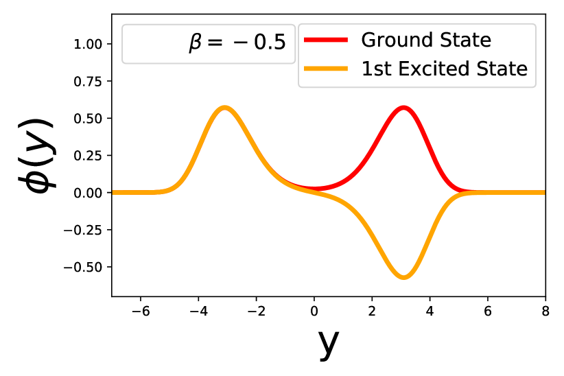
(a)

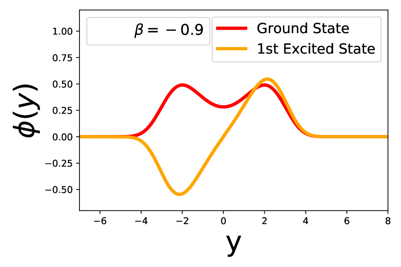
(b)

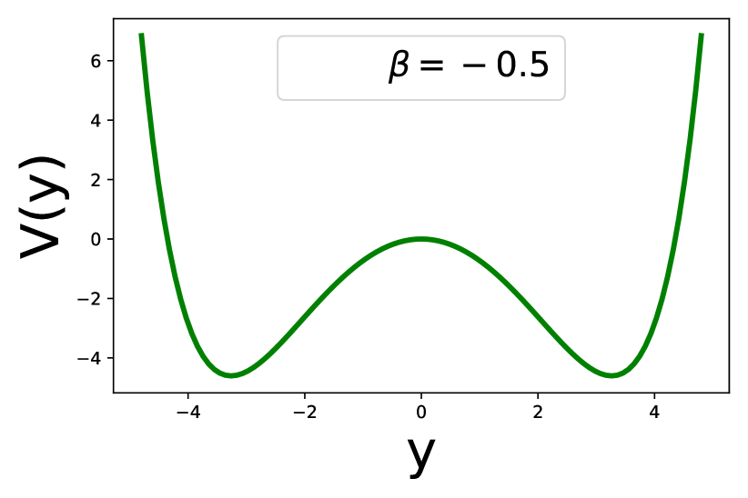
(c)

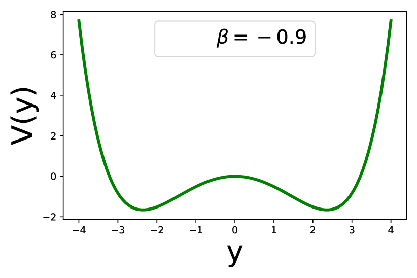
(d)

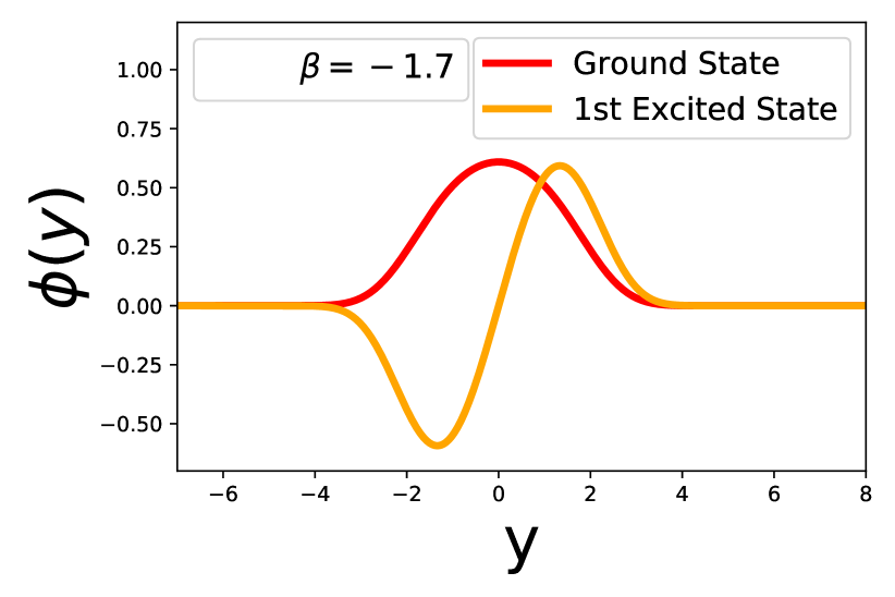
(e)

(f)

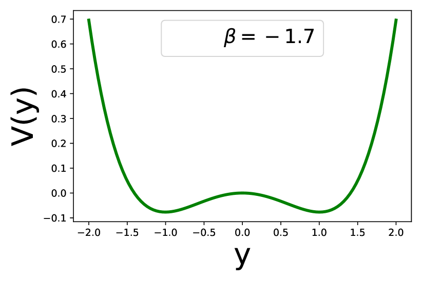
(g)

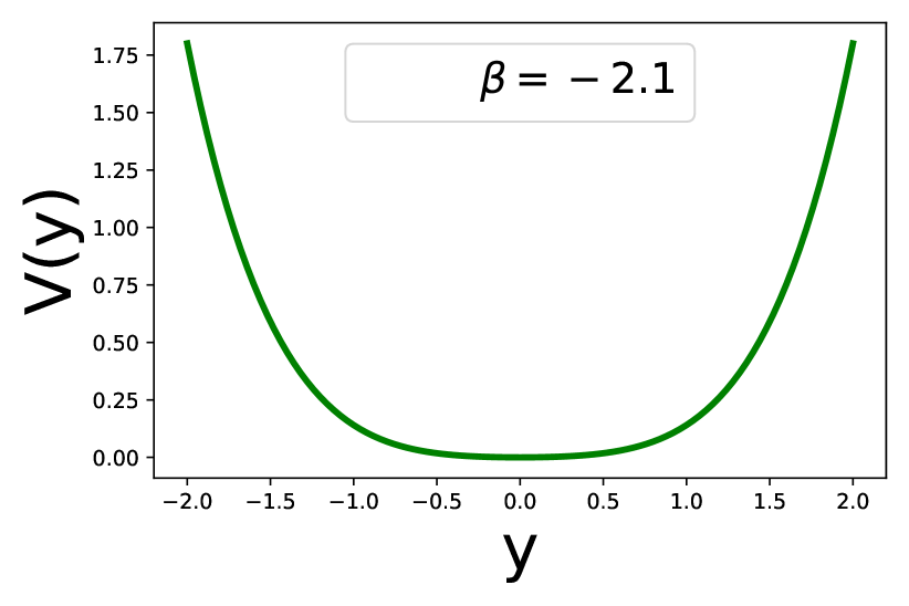
(h)

Figure 1: (Color online) Plot of wave functions and potential for different values of $\beta$ and $\lambda=1$,. Green, Red and Orange solid lines represent potential, ground state and 1st excited state wave functions, respectively. Fig.(a), Fig.(c) $\beta=-0.5$; Fig.(b),Fig.(d) $\beta=-0.9$; Fig.(e),Fig.(g) $\beta=-1.7$; Fig.(f),Fig.(h) $\beta=-2.1$

The barrier between the two wells increases with the decreasing value of $|\beta|$, and the system decomposes into two independent components separated from each other —the wave function is the set of two split up wave functions. The tunnelling probability of the particle from a well to the other increases with the decrease of the barrier height, and the wave-function of the left and right regions tend to overlap. The standard behaviour of wave-function in a double-well represented by a quatric potential is seen in the present context. The eigen values corresponding to the quantum bound states of the system is shown in the Fig. 2 as a function of $\beta$ for a few low lying states.

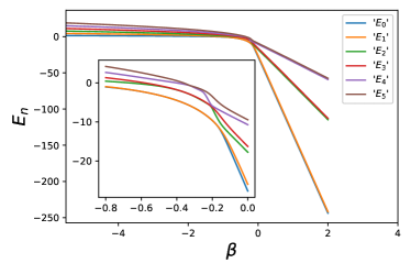
Figure 2: (Color online) Plot of the lowest six energy levels of 2D Toda lattice. Parametric value : $\lambda=1$

We observe that the eigen values come close to each other as $\beta$ increases, although the levels do not cross each other. The degree of level repulsion is low which is obvious for an integrable system. The ground state energy for different values of $\beta$ and $y_{0}$ is shown in the Fig. 3.

Figure 3: (Color online) Plot of ground state energy of 2D Toda lattice for different values of $\beta$ and $y_{0}$. Parametric value : $\lambda=1$

III Periodic Toda lattice with three particles

We consider the following Hamiltonian of a Toda lattice with BLG and VMC for three particles,

$$H = \Pi_{1}\Pi_{2}+\Pi_{1}\Pi_{3}+\Pi_{2}\Pi_{3}+\frac{a}{b}\left[1-e^{b(q_{2}-q_{1})}\right.$$ (10)

$$- \left.e^{b(q_{3}-q_{2})}-e^{b(q_{1}-q_{3})}\right]$$

The generalized momenta appearing in $H$ have the following expressions,

$$\Pi_{1}=p_{1}+\frac{\gamma}{4}(q_{2}+q_{3}),\ \ \Pi_{2}=p_{2}-\frac{\gamma}{4}(q_{1}-q_{3}),$$

$$\Pi_{3}=p_{3}-\frac{\gamma}{4}(q_{1}+q_{2}).$$ (11)

The $\gamma$ dependent terms in $\Pi_{i}$’s produce BLG and VMC in the respective Hamilton’s equations of motion. In particular, the system is governed by the equations of motion,

$$\ddot{q}_{1}+\gamma\dot{q}_{1}+\frac{\gamma}{2}\left(\dot{q}_{2}-\dot{q}_{3}\right)-a\left[e^{b\left(q_{2}-q_{1}\right)}-e^{b\left(q_{1}-q_{3}\right)}\right]=0$$

$$\ddot{q}_{2}+\frac{\gamma}{2}\left(\dot{q}_{1}-\dot{q}_{3}\right)-a\left[e^{b\left(q_{3}-q_{2}\right)}-e^{b\left(q_{2}-q_{1}\right)}\right]=0$$

$$\ddot{q}_{3}-\gamma\dot{q}_{3}+\frac{\gamma}{2}\left(\dot{q}_{1}-\dot{q}_{2}\right)-a\left[e^{b\left(q_{1}-q_{3}\right)}-e^{b\left(q_{3}-q_{2}\right)}\right]=0,$$

where particle-1 and particle-3 are subjected to BLG. Each particle interacts with the remaining two particles via the Toda potential and the VMC. The above classical system has been studied in detail in Ref. proy and shown to admit mixed phases of integrability and chaos —two of the integrals of motion have been obtained analytically. In this article, we study the quantum Hamiltonian $H$ from the view point of its integrability and chaos.

The system is translation invariant. We introduce the Jacobi coordinates $Q_{1},Q_{2},Q_{3}$ in order to separate out the center of mass motion and to work with only two coordinates,

$$Q_{j}=\frac{1}{\sqrt{j(j+1)}}\sum_{k=1}^{j}(q_{k}-jq_{j+1}),Q_{3}=\frac{1}{\sqrt{3}}\sum_{k=1}^{3}q_{k},$$

where $j=1,2$. The momenta $P_{j}$ in the Jacobi coordinates are related to $p_{j}$’s through the same relations —replace $(Q_{k},q_{k})\rightarrow(P_{k},p_{k})$. The Hamiltonian can be rewritten in terms of $(Q_{k},P_{k})$ as,

$$H = \frac{{\tilde{\Pi}_{3}}^{2}}{4}-\frac{\tilde{\Pi}_{1}^{2}}{2}-\frac{\tilde{\Pi}_{2}^{2}}{2}-\frac{a}{b}\left[e^{-b\sqrt{2}Q_{1}}+e^{\frac{b}{\sqrt{2}}(Q_{1}+\sqrt{3}Q_{2})}\right.$$ (12)

$$+ \left.e^{\frac{b}{\sqrt{2}}(Q_{1}-\sqrt{3}Q_{2})}-1\right]$$

where $\tilde{\Pi}_{1}$,$\tilde{\Pi}_{2}$ and $\tilde{\Pi}_{3}$ are the modified generalized momenta:

$$\tilde{\Pi}_{1} = -P_{1}-\frac{\gamma}{4\sqrt{3}}\left(Q_{2}+\sqrt{2}Q_{3}\right)$$

$$\tilde{\Pi}_{2} = -P_{2}+\frac{\gamma}{4\sqrt{3}}\left(Q_{1}-\sqrt{6}Q_{3}\right)$$

$$\tilde{\Pi}_{3} = 2P_{3}-\frac{\gamma}{\sqrt{6}}\left(Q_{1}+\sqrt{3}Q_{2}\right)$$ (13)

The Hamiltonian is not positive-definite even for $\frac{a}{b}<0$.

We quantize the Hamiltonian (12) by replacing $(Q_{j},P_{j})$ with the corresponding operators $(Q_{j},-i\partial_{Q_{j}})$ satisfying the commutation relations $[Q_{j},P_{l}]=i\delta_{jl}$, $[Q_{j},Q_{l}]=0$, $[P_{j},P_{l}]=0$, and denote the resulting Hamiltonian as $\widehat{H}$. We are working with $\hbar=1$. The translation invariance leads to a conserved quantity and the corresponding operator

$$\widehat{\Pi}=-2\sqrt{3}i\frac{\partial}{\partial Q_{3}}+\frac{\gamma}{\sqrt{2}}(Q_{1}+\sqrt{3}Q_{2})$$ (14)

commutes with the Hamiltonian $\widehat{H}$. The complete integrability requires three integrals of motion. However, we have found analytic expressions for two conserved quantities, namely, $\widehat{H}$ and $\widehat{\Pi}$. It will be seen later that numerical investigations indicate integrability of the system in some ranges of the parameter $\gamma$. The commutation relation $[\widehat{H},\widehat{\Pi}]=0$ allows us to find simultaneous wave function of these two operators,

$$\psi(Q_{1},Q_{2},Q_{3}) = \exp\left[\frac{i}{2\sqrt{3}}Q_{3}\left\{k-\frac{\gamma}{\sqrt{2}}\left(Q_{1}\right.\right.\right.$$ (15)

$$+ \left.\left.\left.\sqrt{3}Q_{2}\right)\right\}\right]\phi(Q_{1},Q_{2}),$$

where $k$ is the eigen value of the operator $\widehat{\Pi}$. Inserting the expression of $\psi(Q_{1},Q_{2},Q_{3})$ into the time-independent schrödinger equation $\widehat{H}\psi=\epsilon\psi$, we get an eigen value equation in terms of an effective Hamiltonian $H_{\textrm{eff}}$ and energy E as $H_{\textrm{eff}}\phi=E\phi$, where $E=-(\epsilon-\frac{a}{b})$. The expression of effective Hamiltonian is as follows,

$$H_{\textrm{eff}} = \frac{1}{2}\left(P_{1}+\frac{\gamma}{4\sqrt{3}}Q_{2}\right)^{2}+\frac{1}{2}\left(P_{2}-\frac{\gamma}{4\sqrt{3}}Q_{1}\right)^{2}+V_{\textrm{eff}}$$

$$V_{\textrm{eff}} = -\frac{\gamma^{2}}{6}\left(Q_{1}+\sqrt{3}Q_{2}+\frac{k}{\sqrt{2}\gamma}\right)^{2}+\frac{a}{b}\left[e^{-b\sqrt{2}Q_{1}}\right.$$ (16)

$$+ \left.e^{\frac{b}{\sqrt{2}}(Q_{1}+\sqrt{3}Q_{2})}+e^{\frac{b}{\sqrt{2}}(Q_{1}-\sqrt{3}Q_{2})}\right],$$

where $P_{1},P_{2},Q_{1},Q_{2}$ are to be treated as quantum mechanical operators as mentioned earlier. The effective Hamiltonian may be interpreted as describing a particle moving in a two-dimensional potential $V_{\textrm{eff}}$ and subjected to uniform “fictitious magnetic field”ds2 ; ds3 ; pkg1 perpendicular to the “$Q_{1}-Q_{2}$”-plane with the absolute magnitude $\frac{|\gamma|}{2\sqrt{3}}$. In the terminology of the quantization of system with uniform magnetic field, the “fictitious gauge-potential” in $H_{\textrm{eff}}$ is written in the symmetric gaugeds3 . One may choose the Landau gauge and the corresponding Hamiltonian $H_{L}$ is obtained through a gauge transformation as,

$$H_{L} = exp(-\frac{i\gamma}{4\sqrt{3}}Q_{1}Q_{2})\ H_{\textrm{eff}}\ exp(\frac{i\gamma}{4\sqrt{3}}Q_{1}Q_{2})$$ (17)

$$= \frac{1}{2}(P_{1}+\frac{\gamma}{2\sqrt{3}}Q_{2})^{2}+\frac{P_{2}^{2}}{2}+V_{\textrm{eff}}$$

A quadratic potential arises in $V_{\textrm{eff}}$ as the effect of the BLG and VMC, and the standard Toda potential gets modified. The potential is bounded for $\frac{a}{b}>0$ and contour-plots of the same are shown in Fig. (4) for a few choices of the parameters. We study bound states of the quantum Hamiltonian $H_{\textrm{eff}}$. The analytical treatment of the general eigen value problem appears to be non-trivial, and will be studied numerically. However, exact solutions may be obtained in the limiting case in which the Toda potential is approximated as that of coupled oscillators.

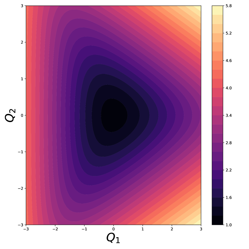
(a)

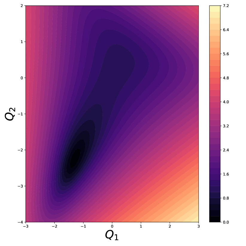
(b)

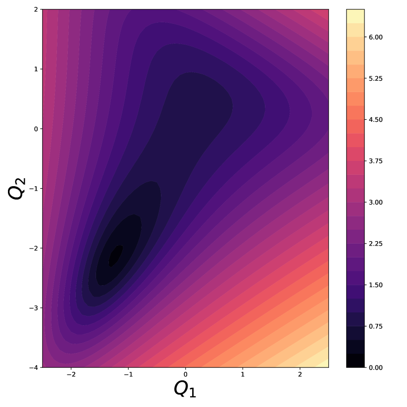
(c)

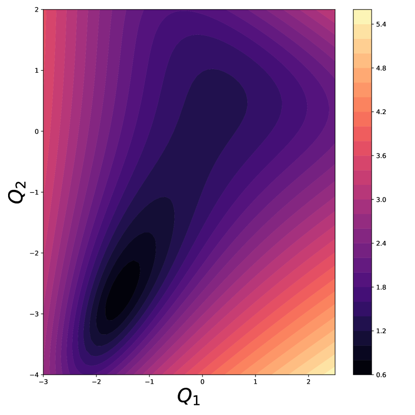
(d)

Figure 4: (Color online) Contour plot of $log(V_{\textrm{eff}})$ for $k=0$. (a) $a=b=1$,$\gamma=0.2$; (b) $a=b=1$,$\gamma=1.6$; (c) $a=0.8$,$b=1$,$\gamma=1.4$; (d) $a=1$,$b=0.8$,$\gamma=1.4$

III.1 A Limiting Case

The Toda potential reduces to that of coupled oscillators in the limit $b\rightarrow 0,a\rightarrow\infty$ such that $ab\equiv\omega^{2}$. The Hamiltonian $H_{\textrm{eff}}$ in this limit reduces to a two-dimensional anisotropic oscillator in an external uniform magnetic field,

$$\tilde{H} = \frac{1}{2}\left(P_{1}+\frac{\gamma}{4\sqrt{3}}Q_{2}\right)^{2}+\frac{1}{2}\left(P_{2}-\frac{\gamma}{4\sqrt{3}}Q_{1}\right)^{2}$$ (18)

$$+ \frac{9\omega^{2}-\gamma^{2}}{6}Q_{1}^{2}+\frac{3\omega^{2}-\gamma^{2}}{2}Q_{2}^{2}-\frac{\gamma^{2}}{\sqrt{3}}Q_{1}Q_{2},$$

where we have taken $k=0$ and dropped the constant term $\frac{3a}{b}$. The term $Q_{1}Q_{2}$ can be removed through a rotation by an angle thirty degree in the anti-clockwise direction. In particular, the transformation

$$Q_{1}=\frac{\sqrt{3}}{2}X+\frac{1}{2}Y,\ Q_{2}=-\frac{1}{2}X+\frac{\sqrt{3}}{2}Y$$ (19)

transforms $\tilde{H}$ to the following form:

$$\tilde{H}=\frac{1}{2}\left(\Pi_{X}^{2}+\Pi_{Y}^{2}\right)+\frac{1}{2}\omega_{1}^{2}X^{2}+\frac{1}{2}\omega_{2}^{2}Y^{2}$$

$$\Pi_{X}={P_{X}+\frac{\gamma}{4\sqrt{3}}Y,\ \Pi_{Y}=P_{Y}-\frac{\gamma}{4\sqrt{3}}X},$$ (20)

where $P_{X}=-i\partial_{x},P_{Y}=-i\partial_{Y}$ and $\omega_{1}^{2}=3\omega^{2},\omega_{2}^{2}=\omega_{1}^{2}-\frac{4\gamma^{2}}{3}$. The Hamiltonian $\tilde{H}$ is $\mathcal{PT}$-symmetric where the parity transformation $\mathcal{P}:(X,Y)\rightarrow(X,-Y),(P_{X},P_{Y})\rightarrow(P_{X},-P_{Y})$ and time reversal operation $\mathcal{T}:(X,Y)\rightarrow(X,Y),(P_{X},P_{Y})\rightarrow(-P_{X},-P_{Y})$. Phase transition occurs in this systems at $9\omega^{2}=4\gamma^{2}$. The eigen values of the systems are real for $\omega^{2}>\frac{4}{9}\gamma^{2}$ and the system is in unbroken $\mathcal{PT}$-symmetric phase. The $\mathcal{PT}$-symmetry is broken for $\omega^{2}<\frac{4}{9}\gamma^{2}$ and the eigen values become imaginary. The Hamiltonian $\tilde{H}$ describes an anisotropic two dimensional harmonic oscillator in an external uniform magnetic field which has been studied earliergui ; rebane . We follow the method outlined in Ref. susy to obtain the eigenspectra. Define a four dimensional vector $U=\left(\omega_{1}X,\Pi_{X},\omega_{2}Y,\Pi_{Y}\right)$ in the phase-space such that $\tilde{H}=\frac{1}{2}UU^{T}$, where $U^{T}$ denotes the transpose of $U$. It may be noted that $\left[U_{i},U_{j}\right]=iM_{ij}$ where the $4\times 4$ matrix $M$ is given by,

$$M=\begin{pmatrix}0&\omega_{1}&0&0\\ -\omega_{1}&0&0&\frac{\gamma}{2\sqrt{3}}\\ 0&0&0&\omega_{2}\\ 0&-\frac{\gamma}{2\sqrt{3}}&-\omega_{2}&0\end{pmatrix}.$$ (21)

The eigenvalues of $iM$ are $(\Omega_{+},-\Omega_{+},\Omega_{-},-\Omega_{-})$ where

$$\Omega_{\pm}=\sqrt{3\left[\omega^{2}\pm\frac{5\gamma}{24}\sqrt{\gamma^{2}+\frac{16}{25}\omega^{2}}-\frac{5}{24}\gamma^{2}\right]},$$ (22)

and reality of $\Omega_{\pm}$ is ensured for $\omega^{2}>\frac{4}{9}\gamma^{2}$. The determinant of the matrix $iM$ is zero for $\omega^{2}=\frac{4}{9}\gamma^{2}$ and $\omega=\pm\frac{2}{3}\gamma$ characterizes a critical phase for which $\Omega_{-}=0$. There exists an orthogonal transformation $V=O^{T}U$ such that the matrix $M$ can be block-diagonalized asstopo ,

$$M_{B}=O^{T}MO=\begin{pmatrix}0&\Omega_{+}&0&0\\ -\Omega_{+}&0&0&0\\ 0&0&0&\Omega_{-}\\ 0&0&-\Omega_{-}&0\end{pmatrix}.$$ (23)

where $O$ is an $O(4)$ rotation matrix and $O^{T}$ is the transpose of $O$. The expression of $O$ is given as,

$$O=\begin{pmatrix}\frac{\sqrt{2}\omega_{1}a_{+}}{\Omega_{+}}({\omega_{2}}^{2}-{\Omega_{+}}^{2})&0&\frac{\sqrt{2}\omega_{1}a_{-}}{\Omega_{-}}({\omega_{2}}^{2}-{\Omega_{-}}^{2})&0\\ 0&\sqrt{2}a_{+}({\omega_{2}}^{2}-{\Omega_{+}}^{2})&0&\sqrt{2}a_{-}({\omega_{2}}^{2}-{\Omega_{-}}^{2})\\ 0&-\frac{\omega_{2}\gamma a_{+}}{\sqrt{6}}&0&-\frac{\omega_{2}\gamma a_{-}}{\sqrt{6}}\\ \frac{\gamma a_{+}\Omega_{+}}{\sqrt{6}}&0&\frac{\gamma a_{-}\Omega_{-}}{\sqrt{6}}&0\end{pmatrix},$$ (24)

where

$$a_{\pm}=\frac{\Omega_{\pm}}{\sqrt{(\omega_{2}^{2}-{\Omega_{\pm}}^{2})^{2}({\omega_{1}}^{2}+{\Omega_{\pm}}^{2})+\frac{\gamma^{2}{\Omega_{\pm}}^{2}}{12}({\omega_{2}}^{2}+{\Omega_{\pm}}^{2})}}.$$

The matrix $O$ is unique modulo $O(4)$ rotations. We denote $M_{D}=\textrm{diag}(\Omega_{+},-\Omega_{+},\Omega_{-},-\Omega_{-})$ and let $S$ diagonalizes $iM$, i. e. $M_{D}=S^{\dagger}(iM)S$. The similarity transformation can not change eigenvalues and let $T$ diagonalizes $iM_{B}$, i.e. $M_{D}=T^{\dagger}(iM_{B})T$. The matrix $O$ is constructed as $O=ST^{\dagger}$. The transformed variables in the phase space $(x,p_{x},y,p_{y})\equiv(v_{1}/{\sqrt{\Omega_{+}}},v_{2}/{\sqrt{\Omega_{+}}},v_{3}/{\sqrt{\Omega_{-}}},v_{4}/{\sqrt{\Omega_{-}}})$ where $\Omega_{-}\neq 0$, satisfy the standard commutation relations,

$$[x,p_{x}]=i,\ [y,p_{y}]=i,\ [x,y]=0=[p_{x},p_{y}].$$ (25)

The Hamiltonian is expressed in terms of new variables as two decoupled anisotropic harmonic oscillators,

$$\tilde{H}=\frac{\Omega_{+}}{2}\left(p_{x}^{2}+x^{2}\right)+\frac{\Omega_{-}}{2}\left(p_{y}^{2}+y^{2}\right).$$ (26)

The Hamiltonian can be expressed in terms of two sets of annihilation and creation operators as,

$$\tilde{H}=\Omega_{+}\left(a^{\dagger}a+\frac{1}{2}\right)+\Omega_{-}\left(b^{\dagger}b+\frac{1}{2}\right),$$

$$a=\frac{1}{\sqrt{2}}\left(p_{x}-ix\right),\ \ b=\frac{1}{\sqrt{2}}\left(p_{y}-iy\right)$$ (27)

The ground state is determined from the conditions $a\Psi_{0}=0,b\Psi_{0}=0$,

$$\Psi_{0}(x,y)=\frac{2}{\sqrt{\pi}}\ e^{-\frac{1}{2}\left(x^{2}+y^{2}\right)},\ \ E_{0,0}=\frac{\Omega_{+}+\Omega_{-}}{2}.$$ (28)

The energy eigenvalues and the eigenfunctions are,

$$E_{n,m}=\left(n+\frac{1}{2}\right)\Omega_{+}+\left(m+\frac{1}{2}\right)\Omega_{-},\ n,m\in\mathbb{Z}^{\geq 0}$$

$$\Psi_{n,m}(x,y)=\frac{(a^{\dagger})^{n}}{\sqrt{n!}}\frac{(b^{\dagger})^{m}}{\sqrt{m!}}\Psi_{0}(x,y).$$ (29)

The wave-function $\Psi_{n,m}(x,y)$ may be expressed in terms of the original variables through a series of inverse transformations which we do not pursue here. It may be noted that there is a reduction in the phase-space for $\omega^{2}=\frac{4}{9}\gamma^{2}$ for which $\Omega_{-}=0$ and the eigenvalues become infinitely degenerate. The energy eigen values are complex for $\omega^{2}<\frac{4}{9}\gamma^{2}$ and entirely real for $\omega^{2}>\frac{4}{9}\gamma^{2}$.

III.2 General Hamiltonian

The eigen value problem for the Hamiltonian $H_{eff}$ in its full generality seems to be unamenable for an analytical treatment. We study the quantum bound states of $H_{eff}$ numerically, and obtain the energy spectra and wave functions by using finite difference method. The scattering states of $H_{eff}$, if any, have been excluded from our purview of study. We have considered $\gamma>0,k\geq 0$ and $a=b=1$ in the numerical calculation unless otherwise stated explicitly. The eigen values and eigenfunctions thus obtained are analyzed to investigate quantum integrability and chaos in the system. In particular, we study avoid level crossing, probability distribution of wave functions in the semi-classical region, level statistics and gap-ratio distribution in order to study quantum integrability and chaos. It is worth recalling that the system in Ref. proy is integrable for $|\gamma|\lessapprox 1.5$ and chaotic above this critical value. We present numerical results in the following for $\gamma$ varying from zero to values above this critical in order to search for quantum integrable and chaotic region.

III.2.1 Avoided level crossing and probability distribution

The lowest ten energy eigen values of $H_{\textrm{eff}}$ for different values of $\gamma$, and $k=0,a=b=1$ are shown in Fig. 5. The energies corresponding to each state decrease with increasing $\gamma$. The energy levels are highly correlated and repel each other. The avoided level crossing is a signature of quantum chaoshaake , since level-crossing gives rise to the degeneracy in the spectrum, implying symmetry and associated conserved quantities in the system. The avoided level crossing is seen for larger values of $\gamma$ in Fig. 5. The level repulsion is not obvious from the figure for smaller values of $\gamma$, and is shown separately in the inset of Fig. 5 for $1\leq\gamma\leq 1.5$. The dependence of the ground state energy of $H_{\textrm{eff}}+\frac{k^{2}}{12}$ on $\gamma$ and $k$ is shown in Fig. 6. The ground state energy is shifted for $k\neq 0$ by an amount of the order of $-\gamma^{2}k$ and the same behaviour is seen.

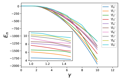
Figure 5: (Color online) Plot of lowest ten energy eigen value of 3-particle system as a function of BLG parameter $\gamma$ for $k=0$ and $a=b=1$

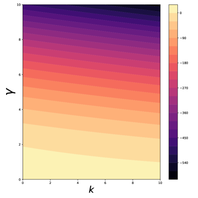
Figure 6: (Color online) Plot of ground state energy for different values of $\gamma$ and $k$. Here $a=b=1$

The Bohr’s correspondence principle allows to make a link between the classical physics and the predictions of quantum mechanics for very high excited states. Thus, a chaotic solution in classical physics should bear some signature in the quantized version of the same system. One of the objects to look for such signatures is the probability distribution of highly excited states. The probability distribution of quantum states of a classically integrable system is expected to be localized in space for low as well as very high quantum numbers. On the other hand, the probability distribution of quantum states corresponding to a classically chaotic system is expected to spread out in space for large values quantum number. The spreading out of the probability distribution for highly excited states can be thought of as the quantum analogue of the chaotic path taken in classical region. We plot the probability distribution of the ground state and a few excited states in Fig. 7 and Fig. 8 for $\gamma=.2$ and $\gamma=1.6$, respectively. It is seen that the probability distribution for $\gamma=0.2$ is localized with uniform distribution for low as well as highly excited states. On the other hand, the complex behaviour arises in the highly excited wave-functions, and manifested in the nonuniform probability distribution for $\gamma=1.6$.

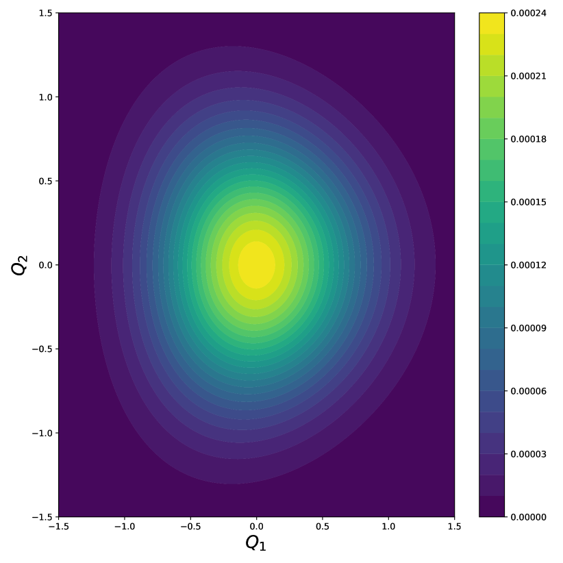
(a)

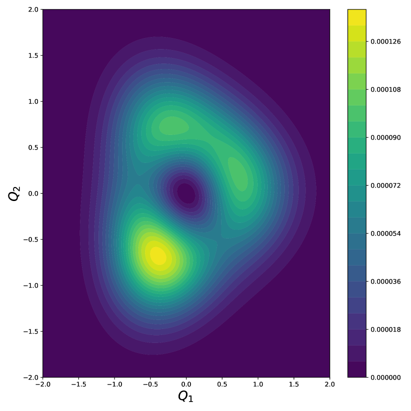
(b)

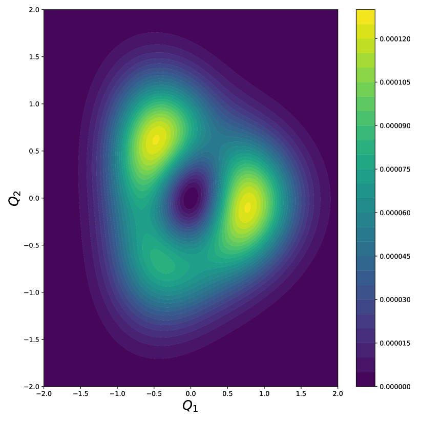
(c)

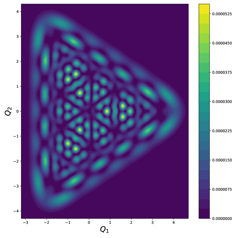
(d)

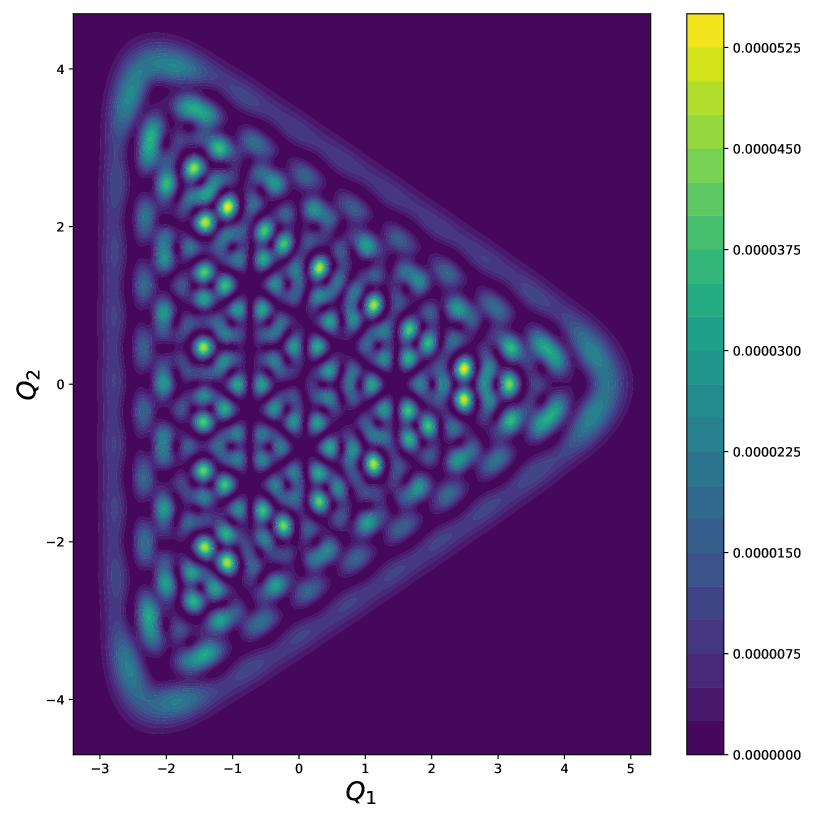
(e)

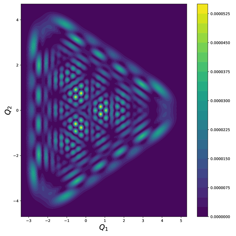
(f)

Figure 7: (Color online) Plot of $|\Phi|^{2}$ for $k=0$,$a=b=1$ and $\gamma=0.2$. (a) Ground state; (b) 1st excited state; (c) 2nd excited state; (d) 200th excited state; (e) 300th excited state; (f) 400th excited state.

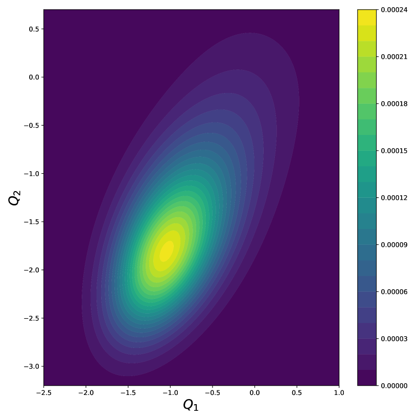
(a)

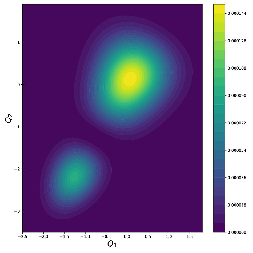
(b)

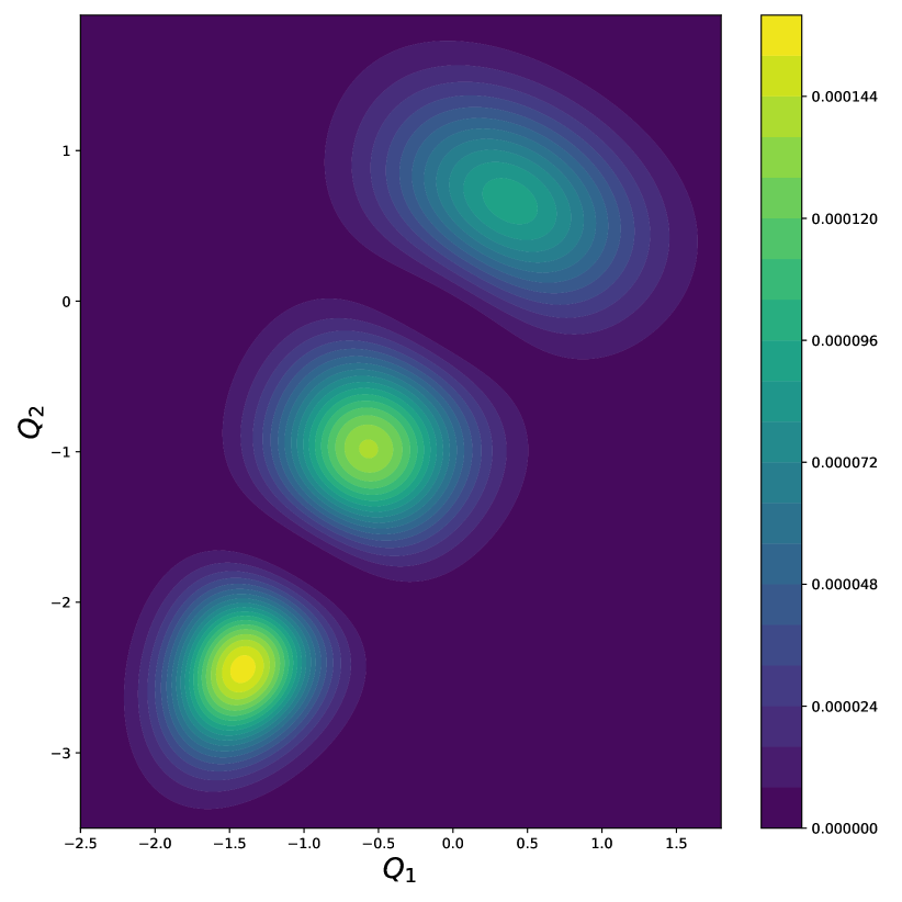
(c)

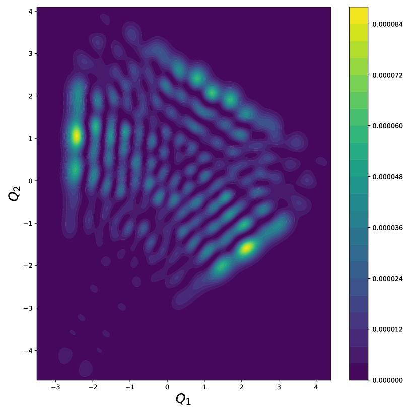
(d)

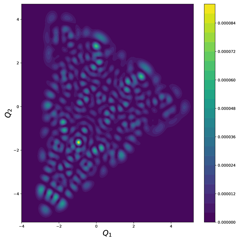
(e)

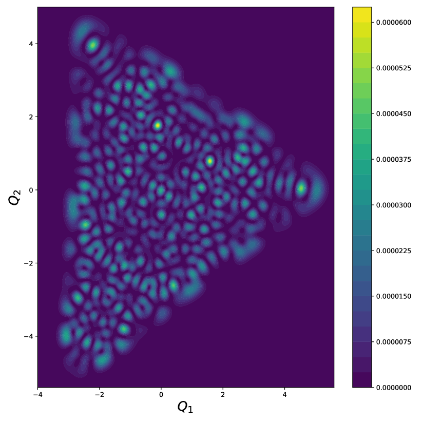
(f)

Figure 8: (Color online) Plot of $|\Phi|^{2}$ for $k=0$,$a=b=1$ and $\gamma=1.6$. (a) Ground state; (b) 1st excited state; (c) 2nd excited state; (d) 200th excited state; (e) 300th excited state; (f) 400th excited state.

III.2.2 Level statistics & Gap-ratio distribution

The chaotic dynamics in classical physics is determined by studying the phase space trajectories, Lyapunov exponents, Poincaré sections etc. The Schrödinger equation being a linear system, the notion of quantum chaos is not uniform, and a quantification of the same is still an active area of research. One of the standard approaches to explore signature of quantum chaos in a classically chaotic system is to study the level statistics. According to the BGS conjecture, the quantum Hamiltonian with chaotic classical dynamics must fall into one of the three classical ensembles of RMTbgs1984 —GOE, Gaussian unitary ensembles(GUE) and Gaussian symplectic ensembles(GSE). The level statistics of quantum Hamiltonian for GOE with integrable classical counterpart follow Poisson law $P_{P}(s)=exp(-s)$, while it follows Wigner distribution $P_{W}(s)=\frac{\pi s}{2}exp\left(-\frac{\pi s^{2}}{4}\right)$ in the classical chaotic region, where $s$ is the spacing of nearest-neighbour eigen-energies berry1977 .

We study level statistics of the eigen spectrum of the Hamiltonian $H_{\textrm{eff}}$. The level spacing distribution is shown by the probability density function $\rho(s)$ of the nearest neighbour spacing of unfolded eigen value. The procedure of unfolding the raw eigen value is a way of locally rescaling the energy spectra such that the mean level density is one. The cumulative spectral function or the staircase function is defined as the number of levels with energy less than or equal to a certain value E. In particular, staircase function is defined as, $N(E)=\sum_{n}\Theta(E-E_{n})$, where $\Theta$ is the unit step function. The function $N(E)$ consists of smooth part $N_{sm}(E)$ and a fluctuating part $N_{fl}(E)$, i. e. $N(E)=N_{sm}+N_{fl}$. We obtain $N_{sm}$ numerically, by fitting the staircase function with a polynomial of degree 15. The unfolded eigen values $x_{i}$ are obtained from raw eigen values $E_{i}$ as $x_{i}=N_{sm}(E_{i})$. Finally The level-spacing distributions are shown by the probability density function $\rho(s)$, where $s=x_{i+1}-x_{i}$.

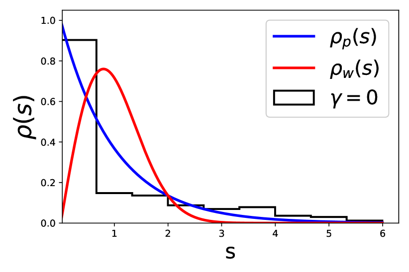
(a)

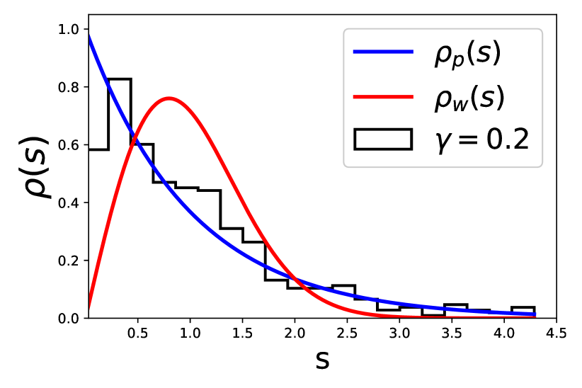
(b)

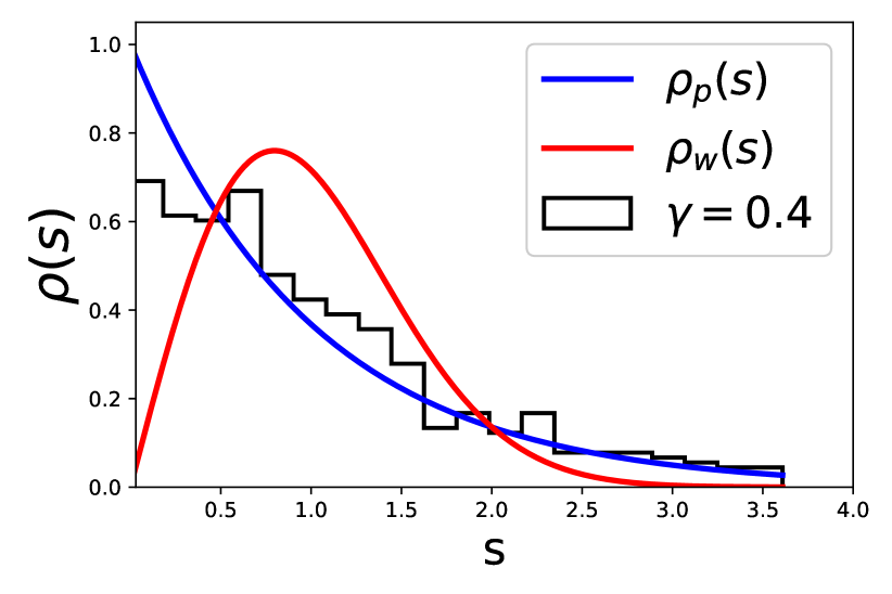
(c)

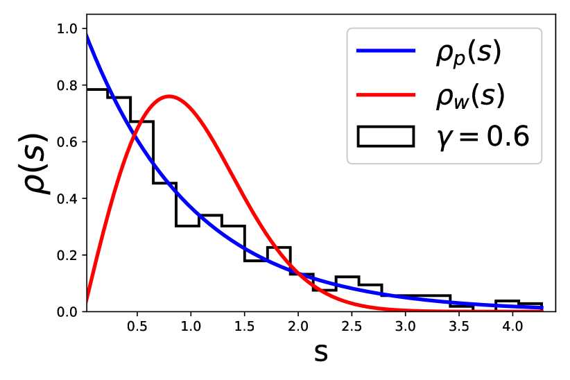
(d)

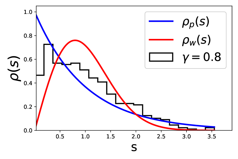
(e)

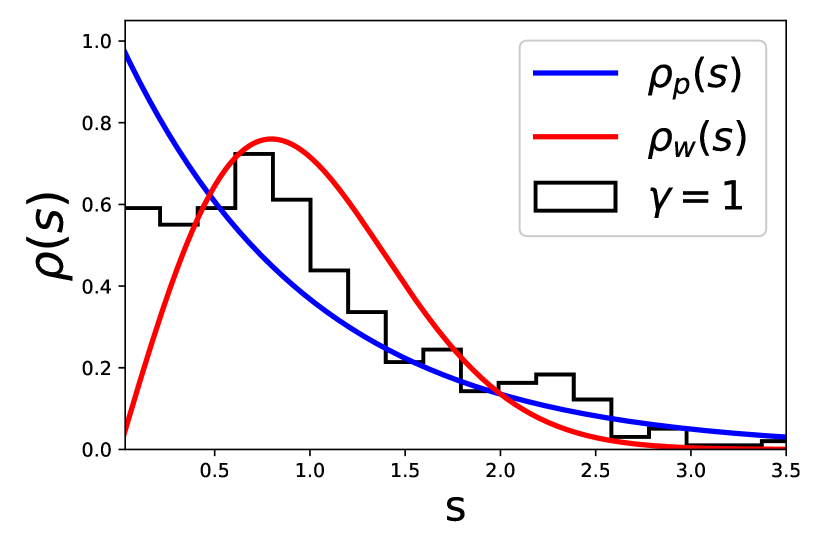
(f)

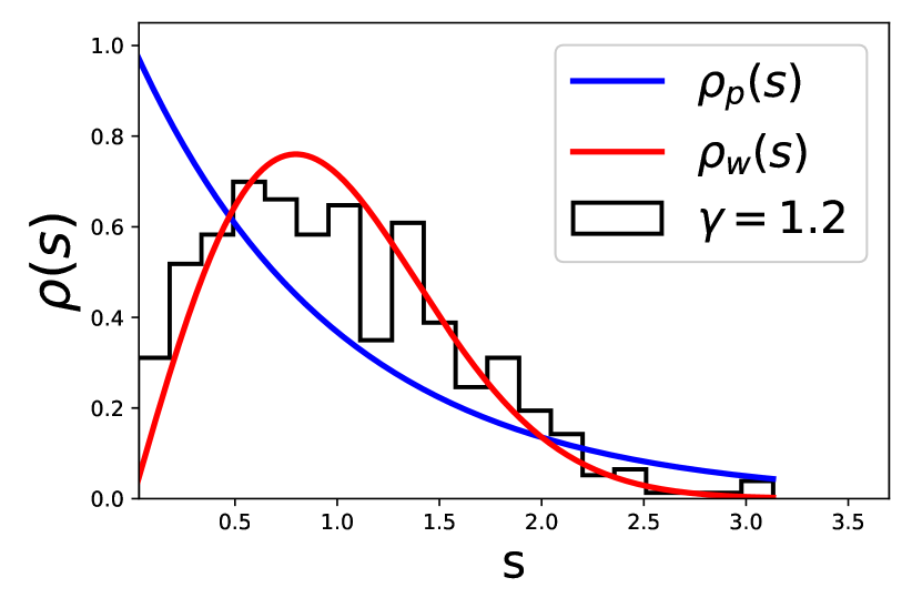
(g)

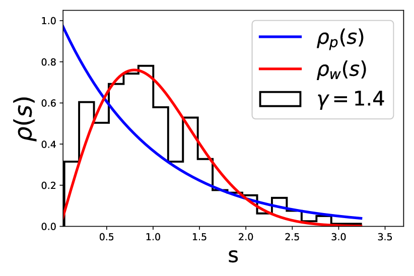
(h)

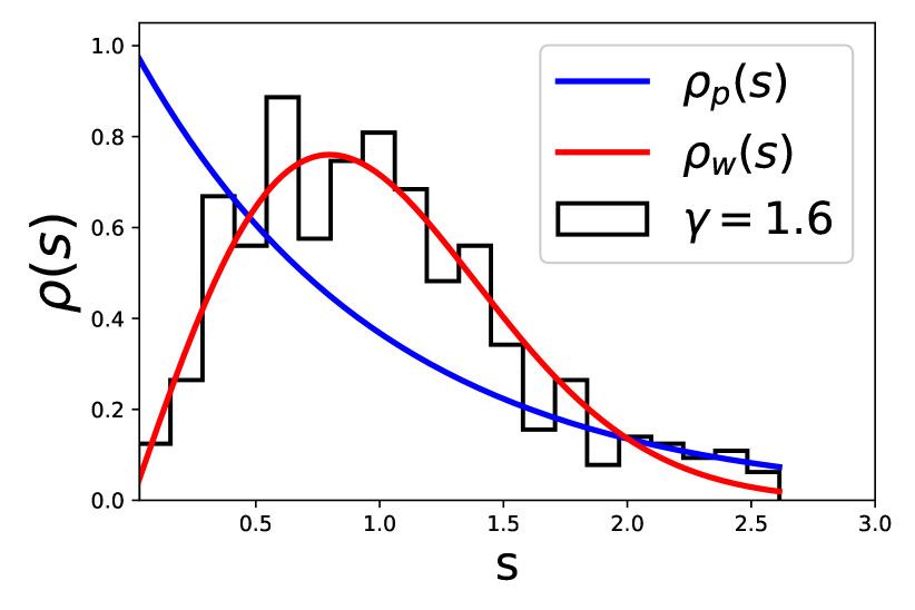
(i)

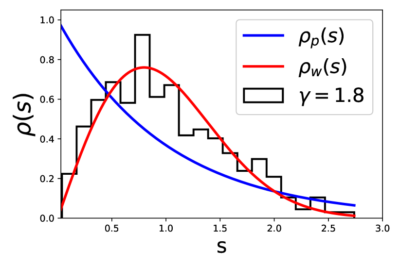
(j)

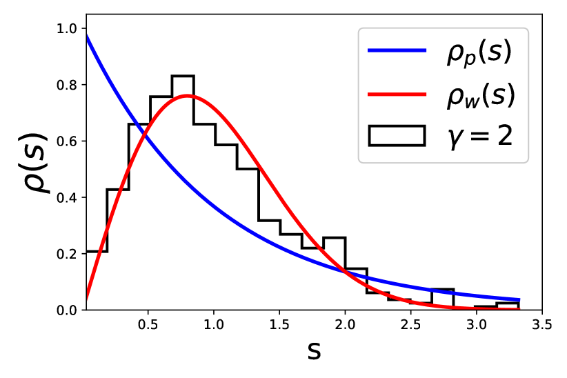
(k)

Figure 9: (Color online) Plot of the level-spacing statistics of Hamiltonian for different values of $\gamma$ and $k=0$,  $a=b=1$. (a) $\gamma=0$; (b) $\gamma=0.2$; (c) $\gamma=0.4$; (d) $\gamma=0.6$; (e) $\gamma=0.8$, (f) $\gamma=1.0$, (g) $\gamma=1.2$, (h) $\gamma=1.4$, (i) $\gamma=1.6$, (j) $\gamma=1.8$, (k) $\gamma=2.0$.

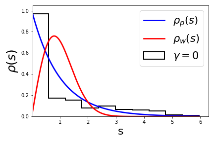
(a)

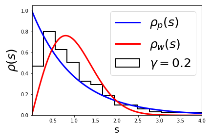
(b)

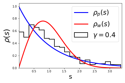
(c)

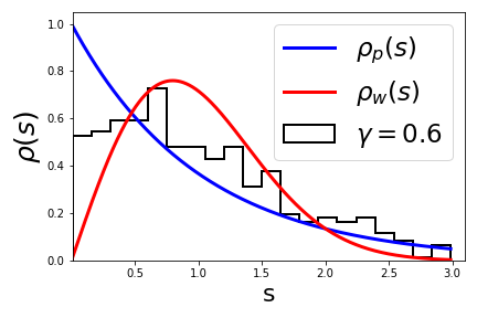
(d)

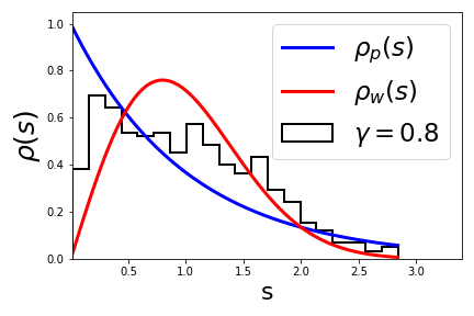
(e)

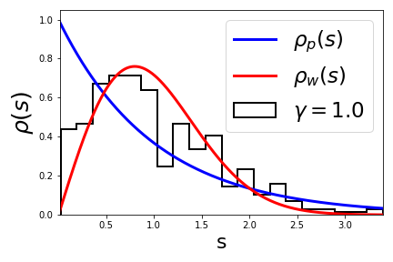
(f)

(g)

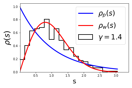
(h)

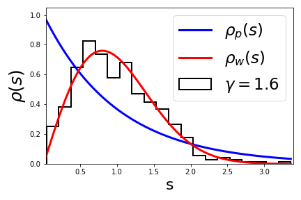
(i)

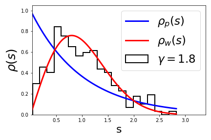
(j)

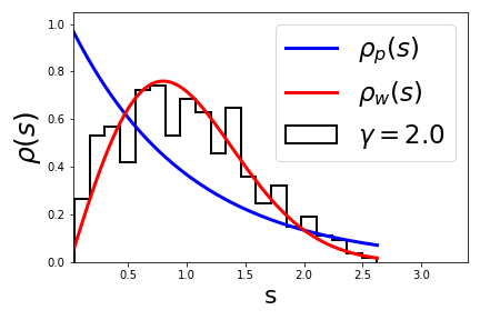
(k)

Figure 10: (Color online) Plot of the level-spacing statistics of Hamiltonian for different values of $\gamma$ and $k=1$ and $a=b=1$. (a) $\gamma=0$; (b) $\gamma=0.2$; (c) $\gamma=0.4$; (d) $\gamma=0.6$; (e) $\gamma=0.8$, (f) $\gamma=1.0$, (g) $\gamma=1.2$, (h) $\gamma=1.4$, (i) $\gamma=1.6$, (j) $\gamma=1.8$, (k) $\gamma=2.0$.

The level spacing distributions of the set of eigen values of the Hamiltonian $H_{\textrm{eff}}$ for different values of $\gamma$ are shown in Fig. 9 and Fig. 10. The blue and red solid lines represent the theoretical graphs for the Poisson and Wigner distributions, respectively. It is seen by comparing Figs. 9 and 10 that the nature of the level spacing distributions are similar for $k=0$ and $k=1$. Further, $\rho(s)$ changes smoothly from the Poisson to Wigner distribution via some intermediate distributions as $\gamma$ is varied from $\gamma=0$ to $\gamma=2$. We define a quantity $\eta$ as follows,

$$\eta=\left|\frac{\int_{0}^{s_{0}}\left[P(s)-P_{W}(s)\right]ds}{\int_{0}^{s_{0}}\left[P_{P}(s)-P_{W}(s)\right]ds}\right|,$$ (30)

where $s_{0}=0.4729......$ is the intersection point of $P_{P}(s)$ and $P_{W}(s)$. It may be noted that $\eta=1$ for $P(s)=P_{P}(s)$, while $\eta=0$ for $P(s)=P_{W}(s)$. Thus, $\eta$ is an indicator of the nature of the distribution, and the plot of the $\eta$ with respect to the parameter $\gamma$ is shown in Fig. 11(a). This diagram in a sense acts as the bifurcation diagram with respect to $\gamma$. The value of $\eta$ approaches one near $\gamma=0$ and goes to zero as $\gamma$ passes through the value $\gamma\approx 1.5$ —the system transits from the integrable to the chaotic region.

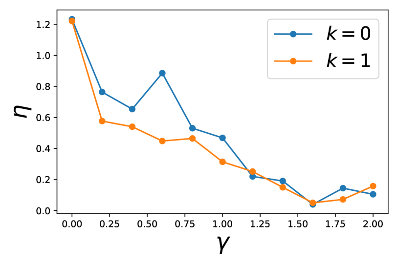
(a)

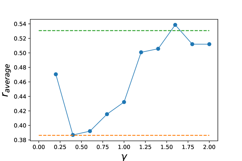
(b)

Figure 11: (Color Online) (a) Plot of $\eta$ with respect to $\gamma$, for $k=0,\ 1$; (b) Plot of $\langle\tilde{r}\rangle$ with respect to $\gamma$ for $k=0$.

The unfolding procedure during the calculation of level statistics is a bit cumbersome and sometime system dependent. The statistics of the ratio of two consecutive energy-gapsoganesyan has been proposed as an alternative measure for the same purpose. The spacing between adjacent energy levels $\delta_{n}=E_{n+1}-E_{n}$, and the ratio between adjacent gaps is defined as,

$$0\leq\tilde{r}_{n}=min\{\delta_{n},\delta_{n-1}\}/max\{\delta_{n},\delta_{n-1}\}\leq 1.$$

The probability distribution of this ratio $\tilde{r}$ for integrable Hamiltonian, $P_{P}(\tilde{r})=\frac{2}{(1+\tilde{r})^{2}}$ and the mean value of this is $\langle\tilde{r}\rangle_{P}=2\ ln2-1\cong 0.386$. The theoretical expression of probability distribution of $\tilde{r}$ in case of $GOE$ ensembles is, $P_{GOE}(\tilde{r})=\frac{27}{4}\frac{\tilde{r}+\tilde{r}^{2}}{(1+\tilde{r}+\tilde{r}^{2})^{2}}$. The mean value in this case, $\langle\tilde{r}\rangle_{GOE}=0.5295\pm 0.0006$.

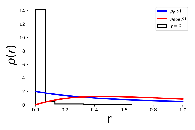
(a)

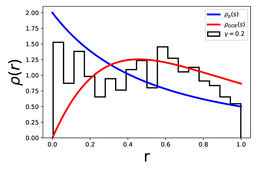
(b)

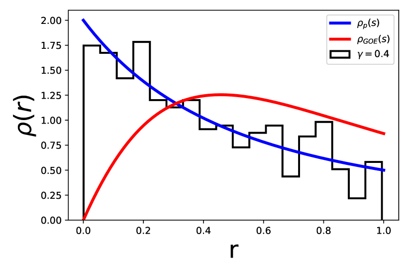
(c)

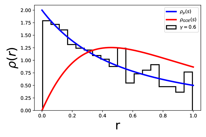
(d)

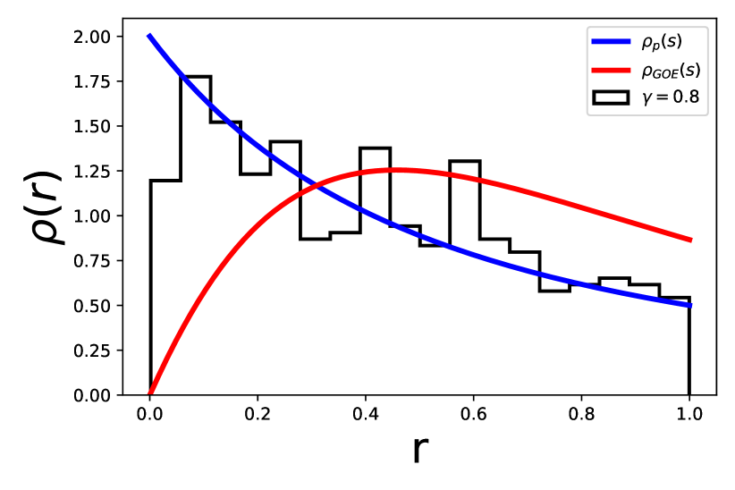
(e)

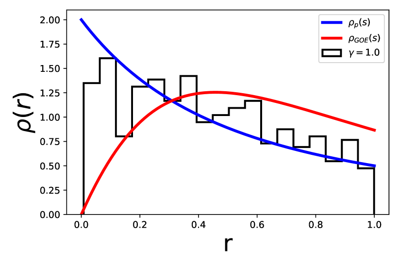
(f)

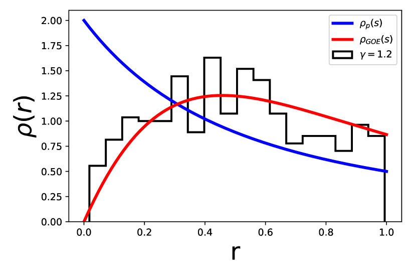
(g)

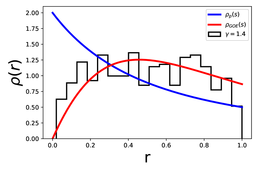
(h)

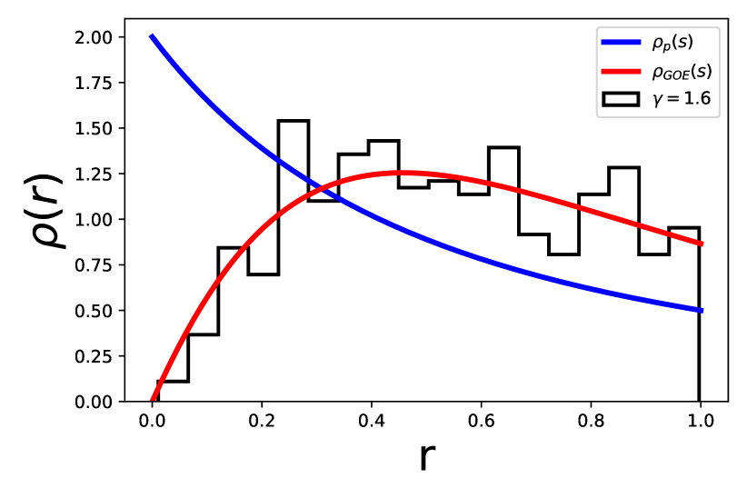
(i)

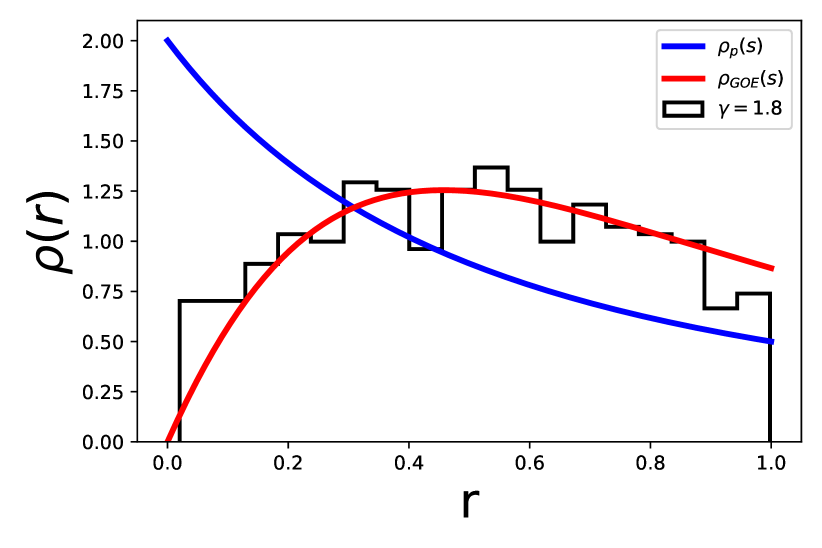
(j)

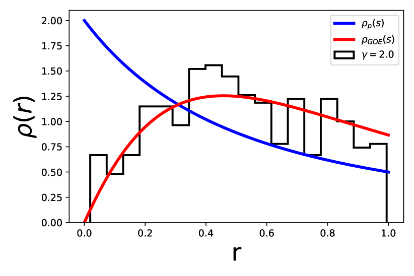
(k)

Figure 12: (Color online) Plot of the Gap Ration $\tilde{r}$ statistics of Hamiltonian with $k=0$,$a=b=1$ for different values of $\gamma$. (a) $\gamma=0$; (b) $\gamma=0.2$; (c) $\gamma=0.4$; (d) $\gamma=0.6$; (e) $\gamma=0.8$, (f) $\gamma=1.0$, (g) $\gamma=1.2$, (h) $\gamma=1.4$, (i) $\gamma=1.6$, (j) $\gamma=1.8$, (k) $\gamma=2.0$.

We study the gap ratio distribution for $k=0$ only because we have already shown that the change in $k$ does not alter the nature of level spacing distribution. The Fig. 12 shows that the probability density distribution of gap ratio $\tilde{r}$ is close to the Poisson distribution up to $\gamma\approx 1.0$. This signifies integrable system. When $\gamma\approx 1.4$ the distribution goes close to the theoretical value of the probability density distribution of GOE ensembles. This signifies the non-integrable region. The Fig. (11(b)) is the bifurcation diagram for this gap ratio distribution. It is see from the bifurcation diagram that while $\gamma\gtrapprox 1.4$ the average value of gap ratio is close to 0.52 i.e. the system is chaotic. We show the quantum transition from integrable to chaotic region by studying nearest neighbour level spacing and gap ratio distribution.

IV Conclusions & Discussions

We have studied the periodic quantum Toda lattice with BLG for two and three particles. The two-particle Toda lattice is integrable and we have constructed two integrals of motion which are in involution. The translation invariance of the system has been used to separate out the center of mass motion, and the effective Hamiltonian in the relative coordinate is described by a particle moving in a potential consisting of harmonic plus cosine hyperbolic. The effective potential describes single or double wells depending on the strength of the loss-gain and the exponential terms. The eigen value equation has been solved numerically, and eigen energies as well as eigenfuntion corresponding to quantum bound states for a few low lying states have been presented. The qualitative behaviour is similar to that of single of double well arising out of a Quartic potential.

The quantum Toda lattice with BLG and VMC for three particles is translation invariant. The effective Hamiltonian after the separation of the center of mass may be interpreted as a particle moving in a two dimensional potential, consisting of anisotropic harmonic oscillators plus Toda potential, and subjected to external uniform magnetic field with its strength being linearly proportional to the strength of the BLG. The angular frequencies of the harmonic oscillators depend quadratically on the strength of the BLG. It has been shown that the effective Hamiltonian is exactly solvable in the limit in which the Toda potential reduces to coupled oscillators. The eigenspectra and eigenfunctions have been obtained analytically by mapping the effective Hamiltonian to that of decoupled anisotropic oscillators in two dimensions via a similarity transformation. There is a limit in which reduction of a degree of freedom occur in phase space and spectra becomes infinitely degenerate.

We have obtained two integrals of motion which are in involution. Although we have not found the third integral of motion which is required to show the complete integrability, the numerical investigations indicates that the three-particle quantum Toda system is integrable below a critical value of the BLG strength and chaotic above this critical value. The quantum integrability and chaos have been investigated via level statistics as well as gap-ratio distribution of the level-spacing of nearest-neighbour eigen values. In particular, we have observed the quantum transition from the chaotic to the integrable region, when the loss-gain strength crosses a critical value and goes to zero —the level spacing as well as the gap-ratio distributions smoothly changes from the Wigner-Dyson distribution and tends to follow the Poisson distribution. We have also studied the level repulsion phenomena in the energy spectra in both the two and three particle Toda lattices. It has been shown through the graphical presentations that the degree of level repulsion is large in the case of the three particle system. The quantum transition from chaotic to integrable region has also been independently confirmed by studying the complexity in higher order excited state wave functions.

There are some immediate questions which may be pursued for future investigations. For example, the analytic expression for the third integral of motion is yet unknown. The standard technique of LAX pair formalism or Painelevé analysis may be employed to find an analytic expression for the same. Further, the generic problem for $N>3$ particles is worth pursuing to see whether or not the mixed phases of intergrability and chaos persist for arbitrary number of particles. It is possible that the system may not be integrable for any range of the strength of the BLG for large $N$. Finally, a semi-classical approach to understand the integrability and chaos is desirable. Some of these issues will be addressed in future publications.

V Acknowledgements

The work of SG is supported by Inspire fellowship(Inspire Code: IF190276) of Govt. of India

References

- (1) M. Toda, Vibration of a Chain with Nonlinear Interaction, Journal of the Physical Society of Japan 22(2), 431, 1967.
- (2) M. Toda, Studies of a non-linear lattice, Phys. Rep. 18, 1 (1975).
- (3) M. Toda, Theory of Nonlinear Lattices, 2nd enl. ed., Springer, Berlin, 1989.
- (4) E. Date and S. Tanaka, Periodic multi-soliton solutions of Korteweg-de Vries equation and Toda lattice, Prog. Theor. Phys. 59, 107 (1976).
- (5) H. Flaschka, The Toda lattice. II. Existence of integrals, Phys. Rev. B 9, 1924 (1974).
- (6) M. Hénon, Integrals of the Toda lattice, Phys. Rev. B 9, 1921 (1974).
- (7) M. A. Agrotis, P. A. Damianou and C. Sophocleous, The Toda lattice is super-integrable, Physica A 365, 235 (2006).
- (8) M. Toda, Solitons and Heat Conduction, Phys. Scr. 20, 424 (1979).
- (9) M. Sataric, J. A. Tuszynski, R. Zakula, and S. Zekovic, Heat conductivity of a perturbed monatomic Toda lattice without impurities, J. Phys.: Condens. Matter 6, 3917 (1994).
- (10) V. Muto, A. C. Scott, and P. L. Christiansen, A Toda lattice model for DNA: Thermally generated solitons, Physica D 44, 75 (1990).
- (11) F. Ovivio, H. G. Bohr, and P. Lindgard, Solitons on H Bond in Proteins, J. Phys.: Con- dens. Matter 15, S1699 (2003).
- (12) G. L. Oppo and A. Politi, Toda potential in laser equations. Z. Phys. B-Condensed Matter 59, 111 (1985).
- (13) Y. Lien, S. M. de Vries, M. P. van Exter, and J. P. Woerdman, Lasers as Toda oscillators, J. Optical Soc. Am. B 19(6), 1461–1466 (2002).
- (14) S. Cialdi, F. Castelli, and F. Prati, Lasers as Toda oscillators: An experimental confirmation, Optics Communications 287, 176 (2013).
- (15) S. Habib, H. E. Kandrup, and M. E. Mahon, Chaos and noise in a truncated Toda potential, Phys. Rev. E 53, 5473 (1996).
- (16) G. Casati and J. Ford, Stochastic transition in the unequal-mass Toda lattice, Phys. Rev. A 12, 1702 (1975).
- (17) L. Vergara and B. A. Malomed, Suppression of the generation of defect modes by a moving soliton in an inhomogeneous Toda lattice, Phys. Rev. E 77, 047601 (2008).
- (18) M. Ezawa, Topological Edge States and Bulk-edge Correspondence in Dimerized Toda Lattice, J. Phys. Soc. Jpn. 91, 024703 (2022).
- (19) P. Roy and P. K. Ghosh, Balanced loss-gain induced chaos in a periodic Toda lattice, Phys. Lett. A 489, 129156(2023).
- (20) P. K. Ghosh, Classical Hamiltonian Systems with balanced loss and gain, J. Phys.: Conf. Ser. 2038, 012012 (2021).
- (21) C. M. Bender, M. Gianfreda, S. K. Ozdemir, B. Peng, and L. Yang, Twofold transition in PT-symmetric coupled oscillators, Phys. Rev. A 88, 062111 (2013).
- (22) C. M. Bender, M. Gianfreda and S. P. Klevansky, Systems of coupled PT-symmetric oscil- lators, Phys. Rev A 90, 022114 (2014).
- (23) Jesús Cuevas, Panayotis G. Kevrekidis, Avadh Saxena, and Avinash Khare, PT-symmetric dimer of coupled nonlinear oscillators, Phys. Rev. A 88, 032108 (2013).
- (24) P. K. Ghosh, Constructing solvable models of vector non-linear Schrödinger equation with balanced loss and gain via non-unitary transformation, Phys. Lett. A 402, 127361(2021).
- (25) S. Ghosh and P. K. Ghosh, Non-linear Schrödinger equation with time-dependent balanced loss-gain and space–time modulated non-linear interaction, Annals of Physics 454, 169330 (2023).
- (26) S. Ghosh and P. K. Ghosh, Solvable limits of a class of generalized vector nonlocal nonlinear Schrödinger equation with balanced loss-gain, Phys. Scr. 98, 115214(2023).
- (27) I. V. Barashenkov and M. Gianfreda, An exactly solvable PT -symmetric dimer from a Hamiltonian system of nonlinear oscillators with gain and loss, J. Phys. A: Math. Theor. 47, 282001 (2014).
- (28) D. Sinha and P. K. Ghosh, -symmetric rational Calogero model with balanced loss and gain, Eur. Phys. J. Plus 132, 460 (2017).
- (29) A. Khare and A. Saxena, Integrable oscillator type and Schrödinger type dimers, J. Phys. A: Math. Theor. 50, 055202 (2017).
- (30) P. K. Ghosh and Debdeep Sinha, Hamiltonian formulation of systems with balanced loss- gain and exactly solvable models, Annals of Physics 388, 276 (2018).
- (31) D. Sinha and P. K. Ghosh, On the bound states and correlation functions of a class of Calogero-type quantum many-body problems with balanced loss and gain, J. Phys. A: Math. Theor. 52, 505203 (2019).
- (32) D. Sinha and P. K. Ghosh, Integrable coupled Liénard-type systems with balanced loss and gain, Annals of Physics 400, 109 (2019).
- (33) P. K. Ghosh and P. Roy, On regular and chaotic dynamics of a non--symmetric Hamiltonian system of a coupled Duffing oscillator with balanced loss and gain, J. Phys. A: Math. Theor. 53, 475202 (2020).
- (34) P. Roy and P. K. Ghosh, Complex dynamical properties of coupled Van der Pol–Duffing oscillators with balanced loss and gain, J. Phys. A : Math. theor. 55, 315701 (2022).
- (35) Pijush K. Ghosh, Taming Hamiltonian systems with balanced loss and gain via Lorentz interaction : General results and a case study with Landau Hamiltonian, J. Phys. A: Math. Theor. 52, 415202 (2019).
- (36) F. Haake, Quantum Signatures of Chaos (Springer-Verlag, Berlin, 1991)
- (37) O. Bohigas, M. J. Giannoni, and C. Schmit, Characterization of Chaotic Quantum Spectra and Universality of Level Fluctuation Laws, Phys. Rev. Lett. 52, 1 (1984).
- (38) M. V. Berry and M. Tabor, Level clustering in the regular spectrum, Proc. R. Soc. Lond. A. 356, 375 (1977).
- (39) G. Montambaux, D. Poilblanc, J. Bellissard, and C. Sire, Quantum Chaos in Spin-Fermion Models, Phys. Rev. Lett. 70, 497 (1993).
- (40) D. Poilblanc, T. Ziman, J. Bellissard, F. Mila, and G. Montambaux, Poisson vs. GOE Statistics in Integrable and Non-Integrable Quantum Hamiltonians, Europhys. Lett., 22 (7), 537 (1993).
- (41) P. van Ede van der Pals and P. Gaspard, Two-dimensional quantum spin Hamiltonians: Spectral properties, Phys. Rev. E 49, 79 (1994).
- (42) B. Georgeot and D.L. Shepelyansky, Integrability and Quantum Chaos in Spin Glass Shards, Phys. Rev. Lett. 81, 5129 (1998).
- (43) K. Kudo and T. Deguchi, Level statistics of XXZ spin chains with a random magnetic field, Phys. Rev. B 69, 132404 (2004).
- (44) T. Deguchi, P. K. Ghosh, and K. Kudo, Level statistics of a pseudo-Hermitian Dicke model, Phys. Rev. E 80, 026213 (2009).
- (45) L. F. Santos and M. Rigol, Onset of quantum chaos in one-dimensional bosonic and fermionic systems and its relation to thermalization, Phys. Rev. E 81, 036206 (2010).
- (46) A. Gubin and L. F. Santos, Quantum chaos: An introduction via chains of interacting spins 1/2, Am. J. Phys. 80, 246 (2012).
- (47) V. Oganesyan and D. A. Huse, Localization of interacting fermions at high temperature, Phys. Rev. B 75, 155111 (2007).
- (48) L. Qiong-Gui, Anisotropic Harmonic Oscillator in a Static Electromagnetic Field, Commun. Theor. Phys. 38, 667 (2002).
- (49) T. K. Rebane, Two Dimensional Oscillator in a Magnetic Field, Journal of Experimental and Theoretical Physics, 114, 220(2012).
- (50) Pijush K. Ghosh, Supersymmetric quantum mechanics on noncommutative space, Eur. Phys. J. C 42, 355(2005).
- (51) D. McDuff and D. Salamon, Introduction to Symplectic Topology, Oxford Science Publications (1998).