UWFormer: Underwater Image Enhancement via a Semi-Supervised Multi-Scale Transformer

Abstract

Underwater images often exhibit poor quality, imbalanced coloration, and low contrast due to the complex and intricate interaction of light, water, and objects. Despite the significant contributions of previous underwater enhancement techniques, there exist several problems that demand further improvement: (i) Current deep learning methodologies depend on Convolutional Neural Networks (CNNs) that lack multi-scale enhancement and also have limited global perception fields. (ii) The scarcity of paired real-world underwater datasets poses a considerable challenge, and the utilization of synthetic image pairs risks overfitting. To address the aforementioned issues, this paper presents a Multi-scale Transformer-based Network called UWFormer for enhancing images at multiple frequencies via semi-supervised learning, in which we propose a Nonlinear Frequency-aware Attention mechanism and a Multi-Scale Fusion Feed-forward Network for low-frequency enhancement. Additionally, we introduce a specialized underwater semi-supervised training strategy, proposing a Subaqueous Perceptual Loss function to generate reliable pseudo labels. Experiments using full-reference and non-reference underwater benchmarks demonstrate that our method outperforms state-of-the-art methods in terms of both quantity and visual quality.

Keywords: Underwater image enhancement, vision transformer, semi-supervised learning, image enhancement

1 Introduction

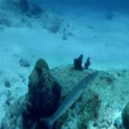
(a) Input

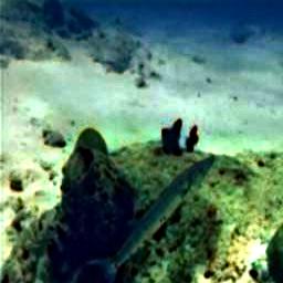
(b) GDCP

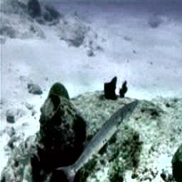
(c) MMLE

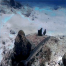
(d) Ucolor

(e) Ours

(f) Target

Figure 1: The figure illustrates a comparison between (a) an underwater image and (f) its enhanced ground truth. Despite the application of (b) traditional enhancement techniques and (c, d) deep learning models, the results still exhibit flaws. By contrast, (e) our method proficiently enhances the image.

Underwater imaging plays a crucial role in the exploration of oceanic ecosystems, the assessment of marine resources, and environmental monitoring. Nevertheless, the quality of underwater images often suffers due to a myriad of factors including light scattering from particle interactions, color cast from light wavelength absorption, turbidity due to suspended particulates, variations in light penetration, the impact of water depth and temperature, motion-induced blurring, and surface disturbances. Consequently, underwater images frequently display diminished clarity, imbalanced coloration, and low contrast. To counter these challenges, a variety of image enhancement techniques have been proposed. These techniques primarily fall into two categories: traditional methods and learning-based solutions [36]. Traditional underwater image enhancement methods typically depend on mathematical models of the underwater environment and prior knowledge like the medium transmission and the dark channel prior [7, 19, 5, 9, 1]. Furthermore, they often necessitate manual input of predefined parameters, which limits their adaptability to varied and dynamic underwater environments, as exemplified in Figure 1 (b).

Learning-based techniques and data-driven methodologies aim to surmount these limitations through direct learning from data. Previous works [8, 39, 24, 12, 22, 21] have demonstrated that superior performance can be attained utilizing deep learning and multi-frequency methods. Nevertheless, most existing methods continue to rely on supervised learning, necessitating extensive paired datasets for model generalization. While training on synthetically generated underwater images [32, 30] could be beneficial, it falls short in effectively capturing the complex characteristics of real-world underwater scenes. Given the limited availability of large paired datasets for underwater image enhancement, it becomes imperative to harness the potential of features within unpaired datasets.

Moreover, existing deep learning-based underwater enhancement techniques rely on CNNs. Although CNNs are adept at capturing local patterns and features within images through their convolutional and pooling layers, they may falter in capturing long-range dependencies and global context. The advent of Vision Transformers [6] allows for the capture of both local and global information. This capacity for cross-positional interaction provides Vision Transformers an edge in managing tasks requiring a broader context and intricate relationships within images. Implementing coarse-to-fine techniques constitutes a viable strategy for optimizing image processing efficiency and alleviating computational resource requirements.

Another significant limitation of these preceding works is the absence of multi-scale enhancement, which becomes particularly important as water interacts with light in a manner that varies depending on the light’s wavelengths. This causes different color spectra to experience distinct attenuation rates during their journey through the water. Consequently, adopting a multi-scale methodology optimized for multiple wavelengths emerges as a more precise strategy for encapsulating the complex interplay of light, water, and objects. Such an approach holds the potential to yield superior image enhancement. To address the aforementioned limitations, this paper offers the following contributions:

1. We introduce UWFormer, a novel semi-supervised Multi-scale Transformer designed to enhance underwater images across multiple frequencies. UWFormer consists of two innovative modules for underwater restoration: the Nonlinear Frequency-aware Attention module and the Multi-scale Fusion Feed-forward network. The incorporation of these two modules fosters frequency-aware attention and varying receptive fields, significantly bolstering the restoration performance.

2. We propose a unique semi-supervised framework for underwater environments. A Subaqueous Perceptual Loss function is employed for generating reliable pseudo labels. This approach enables the teacher’s output to provide a dependable pseudo ground truth for the student model.

3. Comprehensive experiments on 6 benchmark datasets substantiate that our UWFormer outperforms current state-of-the-art methods in terms of visual quality across various underwater scenarios.

2 Related Work

2.1 Traditional Underwater Image Enhancement

The majority of traditional solutions for underwater image enhancement are physics-based [31].

For instance, the model by Ancuti et al. [2], which involves color correction and contrast enhancement, relies on weight mapping and image combination techniques for generating the final output.

Additionally, the MMLE approach[42] utilizes locally adaptive contrast enhancement and color loss minimization to boost image clarity and intensify contrast.

The GDCP method [35] introduces the generalized dark channel prior approach for restoring underwater images. However, in recent years, learning-based methods have gained prominence as superior techniques for enhancing underwater images.

2.2 Learning-based Underwater Image Enhancement

Recent years have witnessed the rapid advancement of learning-based methods.

UGAN  [8] seeks to boost the performance of Autonomous Underwater Vehicles in vision-driven tasks.

UWCNN [16] introduces an underwater image enhancement CNN model based on underwater scene priors.

UColor [17] employs a medium transmission-guided multicolor spatial embedding network to effectively enhance visual quality.

Shallow-UWNet [27] is a lightweight neural network structure that enhances underwater images with fewer parameters.

PWRNet [11] leverages a wavelet boost learning strategy to progressively enhance underwater images in both spatial and frequency domains.

FuineGAN [12] enhances image brightness, contrast, and color balance in real-time, aiding in underwater target detection and identification.

TOPAL [14] proposes an adversarial and perceptually oriented fusion network.

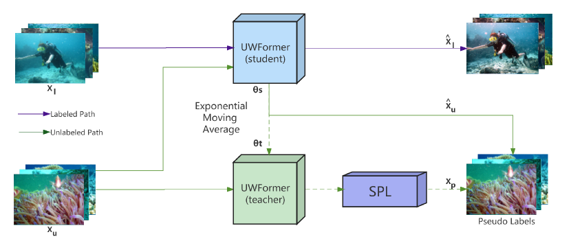
Figure 2: Proposed underwater semi-supervised training strategy. Labeled images $X_{l}\in\mathbb{R}^{C\times H\times W}$ and unlabeled images $X_{u}\in\mathbb{R}^{C\times H\times W}$ are fed to: (i) the student model for training, and (ii) the teacher model for unlabeled prediction. The student model outputs labeled results $\hat{X_{l}}$ and unlabeled results $\hat{X_{u}}$, with the $\hat{X_{l}}$ converging using a supervised loss function. Note that the outputs of the teacher model are evaluated and updated in real-time using the proposed Subaqueous Perceptual Loss (SPL) to generate pseudo labels $X_{p}$. Finally, the unlabeled outputs of the student model $\hat{X_{u}}$ are constrained by $X_{p}$ using an unsupervised loss function. In this case, the weights of the student model are determined by both labeled data and unlabeled data.

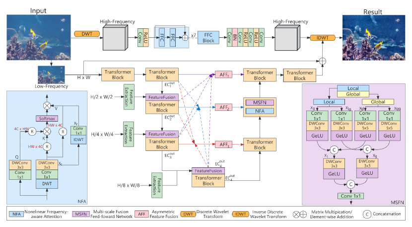
Figure 3: Overall architecture of our proposed UWFormer. An input image $X\in\mathbb{R}^{C\times H\times W}$, it is first processed by DWT to produce three high-frequency images $\left\{X_{LH},X_{HL},X_{HH}\right\}\in\mathbb{R}^{C\times H\times W}$ and one low-frequency image $X_{LL}\in R^{C\times H\times W}$. The three high-frequency images $X_{LH},X_{HL},X_{HH}$ are then merged into a 9-channel image $X_{H}$ and fed into a simple ResNet composed of FFC. The low-frequency part $X_{LL}$ is fed into our MSFormer. Note that the $X_{LL}$ at different scales are subjected to feature extraction and then fed into the MSFormer in a top-down way, where they are fused with the output of the previous encoder. Eventually, the output of the MSFormer $\hat{X_{LL}}$ and the optimized image $\hat{X_{H}}$ are subjected to IDWT to obtain the final result.

3 Methodology

3.1 Overview

The overall architecture of the proposed UWFormer is illustrated in Figure 3. To enable multi-scale enhancement and save computational resources, we adopt lossless downsampling and reconstruction. We utilize the Discrete Wavelet Transform (DWT) and its inverse (IDWT) [26] to enhance individual frequencies using distinct methods. Since high-frequency components, such as texture and edges, often undergo minor alteration [23], we use a simple ResNet composed of Fast Fourier Convolutions to enhance these frequencies. Conversely, we introduce our proposed Transformer architecture to refine low-frequency components, which contain essential color information. This allows for fewer computing resources to be allocated to the high-frequency domain with lower variability, while dedicating more resources to the domain that requires more learning.

3.2 Semi-supervised Training Strategy

The limited availability of labeled underwater enhancement datasets necessitates the integration of unlabeled data to improve performance. To this end, we adopt a mean-teacher based semi-supervised training strategy [33, 10] to learn from both labeled and unlabeled data as illustrated in Figure 2.

Given a labeled underwater image dataset $D_{L}=\left\{\left(x_{i}^{l},y_{i}^{l}\right)\mid x_{i}^{l}\in\mathcal{I}_{s}^{IN},y_{i}^{l}\in\mathcal{I}_{s}^{GT}\right\}_{i=1}^{N}$, where $x_{i}^{l}$ and $y_{i}^{l}$ are the input image set $\mathcal{I}_{s}^{IN}$ and groudtruth set $\mathcal{I}_{s}^{GT}$. Simultaneously, given an unlabeled underwater datset $D_{U}=\left\{x_{i}^{u}\mid x_{i}^{u}\in\mathcal{I}_{u}^{DU}\right\}_{i=1}^{M}$, where $x_{i}^{u}$ indicates the degraded underwater image set $\mathcal{I}_{u}^{DU}$. Our objective is to learn the mapping $M=D_{L}\cup D_{U}\textbf{}$ while ensuring that $D_{L}\cap D_{U}=\emptyset$.

UWFormer comprises two networks with the same structures, referred to as the teacher model and the student model. The primary distinction between the networks lies in how their weights are updated. Specifically, we utilize normal gradient descent to update the student’s weights ($\theta_{s}$), whereas the teacher’s weights ($\theta_{t}$) are updated based on the exponential moving average (EMA) of the student’s weights using the equation described in (1).

$$\theta_{t}=\eta\theta_{t}+(1-\eta)\theta_{s}$$ (1)

the momentum term $\eta\in(0,1)$ is used to indicate the rate of updates made in the EMA update approach. This approach enables the teacher model to incorporate the weights it has learned immediately after each training step. The use of temporal weight averaging stabilizes the training process and enhances performance compared to normal gradient descent, as reported in [29].

Although the teacher network is generally superior to the student network, relying solely on the teacher’s output (pseudo-label) to train the student network on an unidentified dataset can sometimes lead to suboptimal results. To mitigate this risk, we introduce a new loss function Subaqueous Perceptual Loss (SPL) as explained in Section 3.3 to evaluate the teacher output and adjust it in real-time. By doing so, we can treat the teacher’s output as the positive sample $X_{p}$, which provides a reliable pseudo ground truth for the student model.

Our semi-supervised training strategy employs two loss functions: a supervised loss function $L_{sup}$ and an unsupervised loss function $L_{uns}$. For $L_{sup}$, we use the Mean Squared Error $L_{MSE}$, Structural Similarity Index $L_{SSIM}$, and Perceptual Loss $L_{Perc}$ [15] as the loss functions. And the full $L_{sup}$ can be formulated as 2:

$$L_{sup}=L_{MSE}+L_{SSIM}+0.3*L_{Perc}$$ (2)

as given in (3), (4), and (5) respectively.

$$L_{MSE}=\frac{\sum_{\mathrm{i}=1}^{n}(f(x)-y)^{2}}{n}$$ (3)

$$L_{SSIM}=\frac{\left(2\mu_{\mathrm{x}}\mu_{\mathrm{y}}+C_{1}\right)\left(2\sigma_{\mathrm{xy}}+C_{2}\right)}{\left(\mu_{\mathrm{x}}^{2}+\mu_{\mathrm{y}}^{2}+C_{1}\right)\left(\sigma_{\mathrm{x}}^{2}+\sigma_{\mathrm{y}}^{2}+C_{2}\right)}$$ (4)

where $\mu_{\mathrm{x}}$ and $\mu_{\mathrm{y}}$ are the mean of images X and Y, $\sigma_{\mathrm{x}}y$ represents the covariance between images X and Y, $\sigma_{\mathrm{x}}$ and $\sigma_{\mathrm{y}}$ represent the standard deviation of images X and Y. Normally, $C_{1}=(K_{1}\times L)^{2}$ and $C_{2}=(K_{2}\times L)^{2}$ with $K_{1}$, $K_{2}$ and $L$ set to $0.01$, $0.03$ and $255$.

$$L_{\Phi}=\sum^{5}_{k=0}\lambda_{l}||\Phi_{k}(I_{free}^{{}^{\prime}}))-\Phi_{k}(I_{free})||_{1},$$ (5)

where $\Phi$ is the ImageNet-pretrained VGG-16 model. We assess the differences between the CONVk2 ($k=1...5$) and the original pictures ($k=0$ in Equation 5) between the ground truth and the enhanced image.

Regarding the unsupervised loss function, we employ the L1 loss $L_{1}$, and the Contrastive Regularization Loss $L_{cr}$ [10], as given in 7.

$$\mathrm{L}_{1}(\mathrm{\hat{X_{u}}},\mathrm{\hat{X_{p}}})=\sum_{\mathrm{i}=1}^{\mathrm{n}}\mid\mathrm{\hat{X_{u}}}-\mathrm{\hat{X_{p}}}\mid$$ (6)

where $\hat{X_{u}}$ is unlabeled result of student output and $\hat{X_{p}}$ is the positive sample output by teacher model.

$$L_{cr}=\sum_{j=1}^{K}\sum_{i=1}^{M}\omega_{j}\frac{\left|\varphi_{j}\left(\tilde{y}_{i}^{ua}\right),\varphi_{j}\left(y_{i}^{p}\right)\right|}{\left|\varphi_{j}\left(\tilde{y}_{i}^{ua}\right),\varphi_{j}\left(\phi_{s}\left(x_{i}^{ua}\right)\right)\right|}$$ (7)

where $\phi_{s}\left(x_{i}^{ua}\right)$ is the augmented images before being sent to the student model, $\tilde{y}_{i}^{ua}=f_{\theta_{s}}\left(\phi_{s}\left(x_{i}^{ua}\right)\right)$ represents the student output on the unlabeled data, $y_{i}^{p}$ is the positive sample. $\varphi_{j}(\cdot)$ indicates the hidden layer of pretrained VGG-19 and $\omega_{j}$ is the weight coefficient. And the full $L_{uns}$ is written as 8:

$$L_{uns}=L_{1}+L_{cr}$$ (8)

The parameter $\lambda$ represents the current weight of the consistency loss function, which measures the variation in the model’s output under perturbations of the input data. The final objective function is defined as the summation of the labeled loss and the consistency loss, as shown in Equation 9:

$$L_{total}=L_{sup}+\lambda*L_{uns}$$ (9)

3.3 Subaqueous Perceptual Loss

The limited availability of labeled underwater enhancement datasets necessitates the integration of unlabeled data to improve performance. Generally speaking, semi-supervised strategies are suitable for this scenario, but common semi-supervised strategies have not been optimized specifically for underwater augmentation, which may result in ultimately unsatisfactory outcomes. To this end, we introduce a new Subaqueous Perceptual Loss in a special-designed semi-supervised training strategy to learn from both labeled and unlabeled data.

The Subaqueous Perceptual Loss is an underwater quality loss function defined in the CIELab [37, 3] color space that enables the teacher model to produce high-quality reliable pseudo labels, which can be written as Equation 10:

$$SPL=c_{1}\times\sigma_{c}+c_{2}\times\operatorname{c}_{l}+c_{3}\times\mu_{s}$$ (10)

where $c_{1},c_{2},c_{3}$ are weighted coefficients, which are assigned the values 0.4680, 0.2745 and 0.2576 respectively; $\sigma_{c}$ is the chroma standard deviation; $\operatorname{c}_{l}$ is the luminance contrast; $\mu_{s}$ is the average saturation.

3.4 Transformer Architecture

The Vision Transformer model can effectively utilize self-attention to capture both global and local information concurrently, enabling the extraction of global features. This characteristic can be particularly advantageous for enhancing underwater images. Furthermore, coarse-to-fine strategies have been demonstrated to be effective for image enhancement [13, 34, 4]. Accordingly, we propose our Multi-scale Transformer, which stacks Transformers with multi-scale inputs and progressively refines image quality from bottom to top using the coarse-to-fine approach. This multi-scale architecture allows information in the image to flow through the network while tightly integrating low-level and high-level information into a UNet-like structure. The whole process is depicted in Figure 3.

More specifically, the UWFormer model contains four blocks for the feature extraction process at the start and four blocks for the feature reconstruction process at the end of the network. The model consists of a UNet architecture that has been optimized for multi-scale structures, with each block comprised of a Nonlinear Frequency-Aware Attention (NFA) layer and a Multi-Scale Fusion Feed-forward Network (MSFN). In the middle of the network are four encoders and three decoders, with a progressive increase in the number of blocks in each encoder and a progressive decrease in the number of blocks in each decoder. At each scale, we input $X_{1}\in\mathbb{R}^{C\times H/2\times W/2}$, $X_{2}\in\mathbb{R}^{C\times H/4\times W/4}$ and $X_{3}\in\mathbb{R}^{C\times H/8\times W/8}$ in addition to the original input image, $X\in\mathbb{R}^{C\times H\times W}$. Before being fed into each scale’s encoder, the images undergo feature extraction using a convolution-based process and are then concatenated with the output of the previous encoder.

3.4.1 Nonlinear Frequency-Aware Attention

Researchers like [38] have proposed to downsample and reconstruct feature maps in attention mechanism. However, relying on linear layers for learning image information may lead to the inability of the model to capture the non-linear patterns present in images, potentially leading to issues like overfitting and the presence of excessive parameters. To address this issue, we propose a new module called Nonlinear Frequency-aware Attention. In this module, we replace the conventional linear layers with simple convolutional layers and apply DWT and IDWT to enable lossless downsampling and reconstruction of the feature map. This results in a significant improvement of multi-scale enhancement for underwater scenarios and enhances the non-linear expressive power of the attention mechanism.

NFA processes the feature map $X\in\mathbb{R}^{C\times H\times W}$ through two pathways. The first pathway generates the Query $Q\in\mathbb{R}^{4C\times H\times W}$ by passing $X$ through a $1\times 1$ and $3\times 3$ Depth-wise convolutional (DWConv) layer. In the second pathway, we concatenate the result of the DWT of $X$ into four frequency domains and apply them to two sets of $1\times 1$ and $3\times 3$ convolutional layers to produce the Key $K\in\mathbb{R}^{16C\times H/2\times W/2}$ and Value $V\in\mathbb{R}^{16C\times H/2\times W/2}$. IDWT is also performed on the locally concatenated contextualized downsampled feature $X_{c}$ as a byproduct, which, according to wavelet theory, preserves every detail of the original input $X$. The Query, Key, and Value are subsequently reshaped into $\hat{Q}\in\mathbb{R}^{4C\times HW}$, $\hat{K}\in\mathbb{R}^{HW\times 4C}$, and $\hat{V}\in\mathbb{R}^{HW\times 4C}$, respectively, for the purpose of matrix multiplication. By implementing this process of DWT-Convolution-IDWT in the NFA, a more robust local contextualization with an enlarged receptive field is achieved.

Finally, we formulate the NFA as Eq.11:

$$\operatorname{NFA}=\operatorname{MultiHead}\left(Q,K,V,X^{r}\right),$$ (11)

$$\operatorname{MultiHead}\left(Q,K,V,X^{r}\right)=\left[head_{0},...,head_{j},X^{r}\right]W^{O},$$

$$head_{j}=\operatorname{Attention}{\left(Q_{j},K_{j},V_{j}\right)}=\operatorname{Softmax}\left(\frac{Q_{j}K_{j}^{T}}{\sqrt{D_{h}}}\right)V_{j}$$

where $\left[\cdot\right]$ stands for concatenation and $W^{O}$ is the transformation matrix.

3.4.2 Multi-Scale Fusion Feed-forward Network

Inspired by FFC, which uses two channels for image processing, we propose the Multi-Scale Fusion Feed-forward Network. Similar to FFC, MSFN is a multi-scale structure comprising two connected pathways - a local pathway performing regular convolutions on specific input feature channels, and a global pathway, which operates larger convolutions in the global domain. Each path acquires diverse knowledge that is mutually complementary, allowing features to be improved at various scales across the network, facilitated by the exchange of information between them. Our design allows us to enhance features at multiple scales, a key benefit of MSFN over other architectures.

The MSFN model is designed to extract both detailed and global information from an underwater feature map $X\in\mathbb{R}^{C\times H\times W}$. Specifically, the local branch of MSFN employs regular $3\times 3$ depth-wise convolution to extract detailed information, resulting in feature maps $X_{ll}$ and $X_{lg}$ with the same dimensions as $X$. On the other hand, the global branch of MSFN utilizes a larger $5\times 5$ convolution kernel to capture more global information, resulting in feature maps $X_{g}$ and $X_{gl}$ of the same size as $X_{l}$ and $X_{lg}$. To integrate the local and global information, the feature maps from both branches are combined in a cross-scale manner.

This process can be represented mathematically as shown in Equation 12, which yields a superior enhancement quality:

$$Y=f_{1x1}\left[\sigma(f_{3\times 3}^{dwc}(X_{l})),\sigma(f_{3\times 3}^{dwc}(X_{g}))\right],$$ (12)

$$X_{l}=\left[\sigma(f_{3\times 3}^{dwc}(X_{ll})),\sigma(f_{5\times 5}^{dwc}(X_{gl}))\right],$$

$$X_{g}=\left[\sigma(f_{3\times 3}^{dwc}(X_{lg})),\sigma(f_{5\times 5}^{dwc}(X_{gg}))\right]$$

where $\sigma(\cdot)$ indicates GeLU activation, $f_{1\times 1}$ is $1\times 1$ convolution, $f_{3\times 3}^{dwc}$ and $f_{5\times 5}^{dwc}$ denote $3\times 3$ and $5\times 5$ depth-wise convolution, $\left[\cdot\right]$ means concatenation.

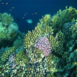
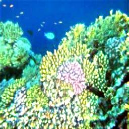
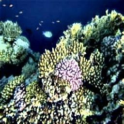
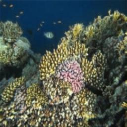
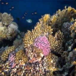
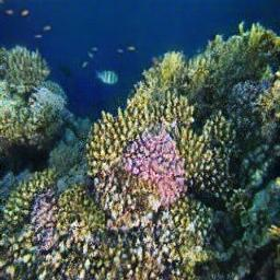
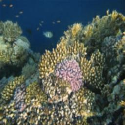
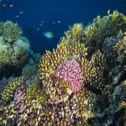
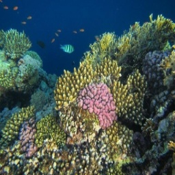
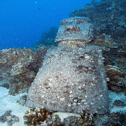
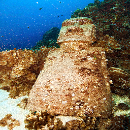
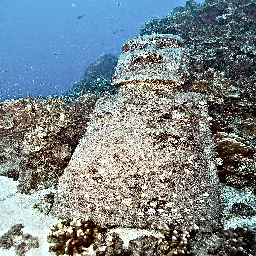
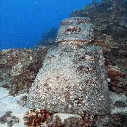
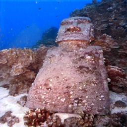
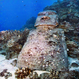
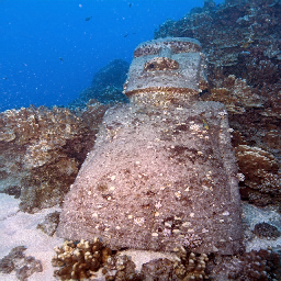
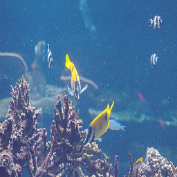
(a)Input

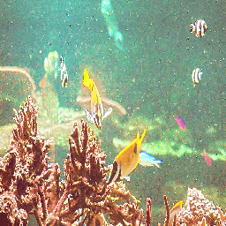
(b)GDCP

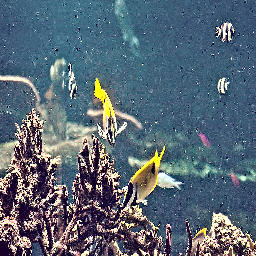
(c)MMLE

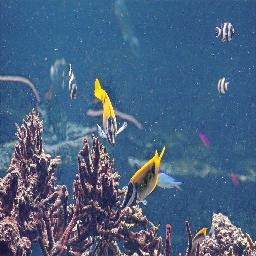
(d)UWCNN

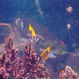
(e)Ucolor

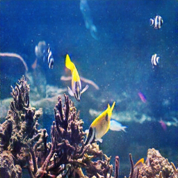
(f)Funie

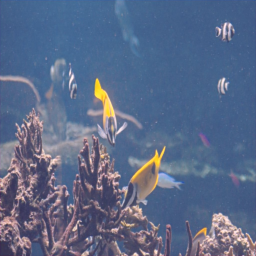
(g)ShallowUW

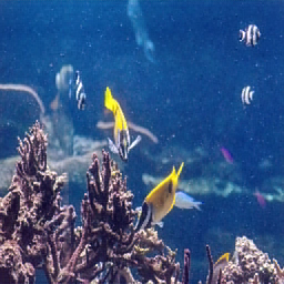
(h)Ours

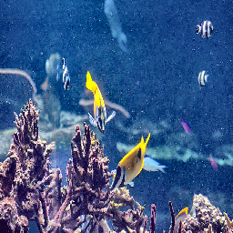
(i)Target

Figure 4: A visual comparison of different image enhancement methods. Methods (b) and (c) show varying degrees of over-optimization, whereas methods (d) and (g) exhibit different degrees of under-optimization. Method (f) shows relatively satisfactory optimization results, yet some optimization defects can still be observed, such as the appearance of white blocks in the middle of the last row. However, our results (h) show superior visual results in terms of color tone and details, and are the closest to the target. The first two rows of images are sourced from EUVP, while the latter two rows are obtained from UIEB.

4 Experiments

4.1 Experiment Settings

In the subsequent section, we provide a comprehensive description of the datasets, evaluation metrics, and implementation specifics. Notably, akin to preceding studies, we do not prioritize network speed in our investigation. Given the consistent test data dimension of $256\times 256$, all methodologies can generate results within a remarkably brief timeframe.

4.1.1 Dataset

The training set for our study comprises 2800 labeled image pairs and 2800 unlabeled images. The labeled dataset, drawn in a 5:2 ratio from EUVP [12] and UIEB [18], includes 890 real-world underwater images from the UIEB dataset, each paired with its corresponding ground truth. The unlabeled images, sourced from EUVPUN [12] and RUIE [25] in an 11:17 ratio, encapsulate a variety of underwater scenes, water types, and lighting conditions, thereby bolstering the generalizability of our model.

For the testing phase, we employ two distinct datasets: full-reference and non-reference. The full-reference dataset encompasses the residual 90 paired images from UIEB and 200 paired images from EUVP. Meanwhile, the non-reference dataset incorporates 1200 images from EUVPUN, all images from U45 [20], the remaining 1930 images from RUIE, and the complete UIEB-60 collection [18]. These datasets, reflecting diverse underwater scenarios, water types, and lighting conditions, provide a robust and comprehensive evaluation of our model’s performance.

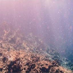
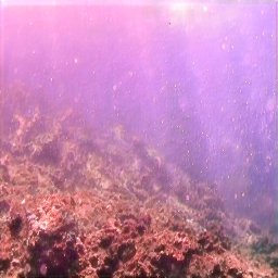
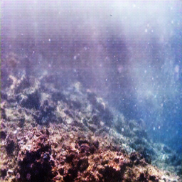
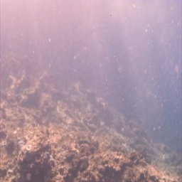
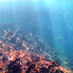
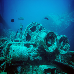
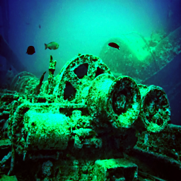
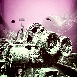
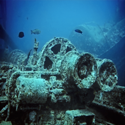
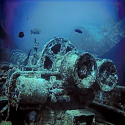
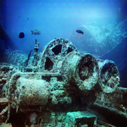
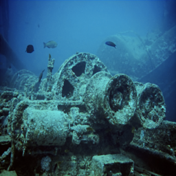
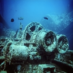
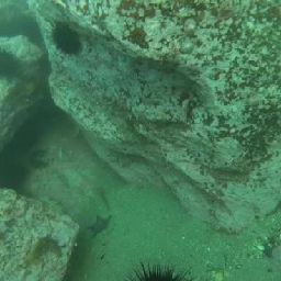
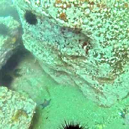
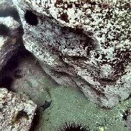
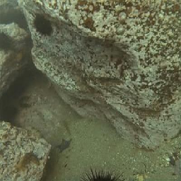
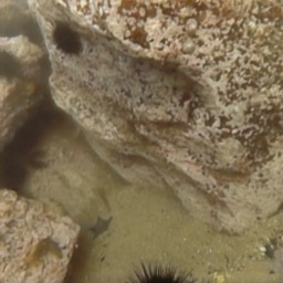
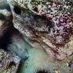
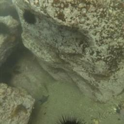
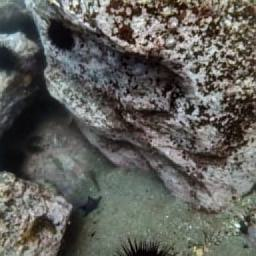
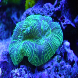
(a)Input

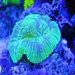
(b)GDCP

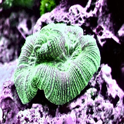
(c)MMLE

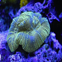
(d)UWCNN

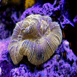
(e)Ucolor

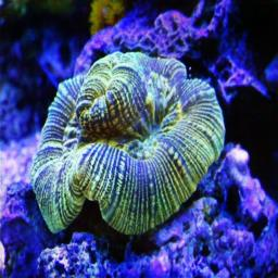
(f)Funie

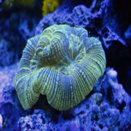
(g)ShallowUW

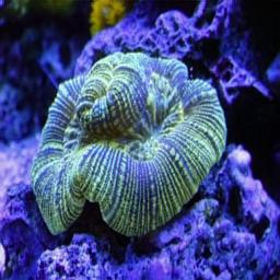
(h)Ours

Figure 5: Visual comparison of different image enhancement methods with no-reference datasets. It shows that methods (b), (c), and (e) exhibit considerable over-enhancement, while methods (d) and (g) do not fully enhance the images. Method (f) shows relatively satisfactory results albeit ambiguous optimization, such as ambiguous optimization in the first row and purple blotches in the third row. Our method (h) provides superior visual results in terms of color tone and details. The images in the rows from top to bottom, respectively originate from UIEB-60, U45, RUIE, and EUVPUN.

Table 1: Quantitative results of comparisons with the state-of-the-art on full-reference datasets. The upper half of the table is the comparison experiment, and the lower half shows the ablation experiment. The best performance is marked in bold.

UIEB EUVP Method PSNR$\uparrow$ SSIM$\uparrow$ LPIPS$\downarrow$ UCIQE$\uparrow$ PSNR$\uparrow$ SSIM$\uparrow$ LPIPS$\downarrow$ UCIQE$\uparrow$ GDCP 14.72 0.745 0.213 0.443 13.10 0.638 0.329 0.427 MMLE 18.24 0.767 0.233 0.441 15.04 0.623 0.269 0.425 UWCNN 18.70 0.841 0.147 0.373 22.98 0.814 0.203 0.388 TOPAL 20.86 0.872 0.109 0.410 20.01 0.801 0.214 0.409 UGAN 21.16 0.787 0.149 0.438 21.58 0.787 0.201 0.424 FunieGAN 19.39 0.802 0.149 0.443 22.06 0.771 0.182 0.418 Ucolor 18.12 0.753 0.228 0.417 20.67 0.786 0.230 0.427 PWRNet 22.50 0.901 0.083 0.427 23.44 0.820 0.208 0.427 ShallowUW 17.66 0.660 0.390 0.354 22.55 0.802 0.205 0.379 UNet 17.93 0.792 0.200 0.389 22.19 0.802 0.212 0.384 W/O SPL 22.12 0.813 0.121 0.401 22.31 0.807 0.171 0.393 MDTA+MSFN 22.61 0.837 0.140 0.402 24.18 0.823 0.151 0.411 NFA+GDFN 22.32 0.831 0.144 0.439 22.56 0.740 0.191 0.425 Supervised 22.72 0.894 0.085 0.413 24.24 0.840 0.155 0.411 Ours 23.23 0.903 0.077 0.446 24.40 0.845 0.129 0.431

Table 2: Quantitative results of comparisons with the state-of-the-art on non-reference datasets. The upper half of the table is the comparison experiment, and the lower half shows the ablation experiment. The best performance is marked in bold, while the second-best performance is underlined.

EUVPUN U45 RUIE UIEB-60 Method UIQM$\uparrow$ UCIQE$\uparrow$ UIQM$\uparrow$ UCIQE$\uparrow$ UIQM$\uparrow$ UCIQE$\uparrow$ UIQM$\uparrow$ UCIQE$\uparrow$ GDCP 2.751 0.420 2.347 0.415 2.706 0.338 2.196 0.393 MMLE 2.737 0.419 2.599 0.423 2.805 0.345 2.197 0.395 UWCNN 2.812 0.374 3.151 0.380 2.580 0.245 2.427 0.338 TOPAL 2.812 0.414 3.165 0.392 2.871 0.287 2.728 0.373 UGAN 2.807 0.438 3.178 0.418 2.882 0.344 2.769 0.394 FunieGAN 2.804 0.440 3.202 0.417 2.802 0.361 2.879 0.401 Ucolor 2.824 0.430 3.042 0.421 2.607 0.275 2.424 0.395 PWRNet 2.806 0.418 3.222 0.423 2.822 0.338 2.700 0.388 ShallowUW 2.824 0.362 2.980 0.348 2.355 0.222 2.379 0.313 UNet 2.485 0.395 2.936 0.378 2.481 0.247 2.406 0.351 W/O SPL 2.718 0.417 3.074 0.403 2.757 0.329 2.726 0.367 MDTA+MSFN 2.723 0.408 3.101 0.401 2.686 0.315 2.711 0.361 NFA+GDFN 2.710 0.403 3.043 0.396 2.711 0.312 2.713 0.391 Supervised 2.658 0.419 3.136 0.403 2.781 0.314 2.718 0.377 Ours 2.831 0.442 3.227 0.440 2.891 0.347 2.789 0.416

4.1.2 Evaluation Metrics

Our study utilizes several full-reference evaluation metrics, namely Peak Signal-to-Noise Ratio (PSNR), Structural Similarity Index (SSIM), and Learned Perceptual Image Patch Similarity (LPIPS) [41].

Regarding non-reference evaluation metrics, we opt for two specific ones. The first is the Underwater Image Quality Metric (UIQM) [28], a metric that takes into account the unique degradation mechanisms and imaging characteristics inherent in underwater images. The second is the Underwater Color Image Quality Evaluation (UCIQE) [37], a linear amalgamation of colorfulness, saturation, and contrast. We select these metrics due to their proven capability to accurately evaluate the quality of underwater images.

4.1.3 Implementation Details

Our model, constructed with PyTorch, is trained employing the Adam optimizer with default parameters, executed on four NVIDIA RTX 8000 GPUs. We utilize a batch size of 4 throughout the 200 epochs of training, with the learning rate being reduced by a factor of 0.1 at the 100th epoch. The training process adheres to a semi-supervised strategy over the course of 200 epochs. Moreover, data augmentation techniques, including random flipping, rotation, cropping, and resizing, are incorporated.

4.2 Comparisons with State-of-the-Arts

We compare our UWFormer model with nine extant state-of-the-art methods, namely GDCP [35], MMLE [42], UWCNN [16], TOPAL [14], UGAN [8], FunieGAN [12], Ucolor [17], PWRNet [11], and ShallowUW [27]. All these methods have been retrained on our datasets for 200 epochs, leveraging their official implementations.

Table 1 delineates the quantitative results derived from the full-reference datasets. The findings demonstrate that our UWFormer surpasses the existing methods in both image similarity and visual quality across the majority of the metrics. The Multi-scale Transformer architecture, providing a larger receptive field during supervised learning, facilitates superior performance in color restoration and detail preservation compared to other methods. The superior efficacy of our proposed method is further depicted in Figure 4, wherein UWFormer yields aesthetically pleasing outcomes, while the methods compared are plagued by issues such as color cast and over-enhancement.

Table 2 articulates the quantitative results garnered from the non-reference datasets. Our UWFormer attains the highest performance for the majority of the metrics, securing the second rank in three metrics within the RUIE and UIEB-60 datasets. Our proposed SPL effectively accomplishes satisfactory performance in semi-supervised learning, while sustaining the performance of supervised learning. It’s noteworthy that generative models may possess a certain advantage for unsupervised tasks. We furnish visual comparisons in Figure 5, which substantiate that our proposed method generates visually gratifying results, surpassing the existing methods.

4.3 Ablation Studies

We conduct ablation studies to evaluate the efficacy of our proposed UWFormer approach, testing its individual components, and replacing NFA and MSFN with MDTA and GDFN, respectively, given their widespread use in Transformer mechanisms. The components are:

1. UNet: Serves as the baseline

2. W/O SPL: Lets the teacher model generate pseudo labels without the application of SPL

3. MDTA+MSFN: Replaces NFA with MDTA [40]

4. NFA+GDFN: Substitutes MSFN with GDFN [40]

5. Supervised: Our complete UWFormer architecture with a fully supervised training strategy

6. Ours: Our complete UWFormer architecture with a semi-supervised training strategy

The outcomes of our ablation studies on the full-reference and non-reference datasets are presented in Tables 1 and 2, respectively. Our complete version surpasses all other variations, with each module making a substantial contribution to the overall performance. Notably, every component proposed in this work enhances performance.

The baseline yields the poorest results. The W/O SPL showcases the effectiveness of the proposed SPL. Our MDTA+MSFN and NFA+GDFN experiments demonstrate the effectiveness of our NFA and MSFN, respectively. The Supervised experiment performs comparably to our full version on the paired dataset, but lags on the non-reference metrics due to the lack of unlabeled data. In conclusion, our full version model exhibits superior performance on both full-reference and non-reference datasets.

Table 3: The user study conduct on full-reference and no-reference datasets ranked several methods, and the results are averaged to determine the rankings. A lower ranking indicates better human subjective evaluation.

Full-reference No-reference Method Ranking Ranking FunieGAN 2.00 1.57 Ucolor 2.88 3.00 PWRNet 4.00 4.00 Ours 1.12 1.42

4.4 User Study

After meticulous deliberation, we select the top three methods, based on our performance metrics, for a user study, the details of which are provided in Table 3. We randomly choose 15 sets of unique images, and 22 participants rate four sets of full-reference and four sets of non-reference results on two criteria for full-reference: (a) Authenticity, and (b) Simulation Effectiveness. These criteria respectively indicate which image mirrors a realistic underwater image most closely and which image is nearest to the target image.

Our rankings are calculated utilizing a weighted average, where lower values corresponded to higher rankings. Our results achieved the top ranking, signifying that our results are the most preferred by the participants.

5 Conclusion

This paper presents UWFormer, an innovative multi-scale Transformer-based network designed to augment images across various frequencies, utilizing a semi-supervised learning strategy. The proposed UWFormer architecture integrates an underwater-specific design that bolsters performance via the amalgamation of a Nonlinear Frequency-aware Attention mechanism and a Multi-scale Fusion Feed-forward network. Moreover, we propose a new loss function, the Subaqueous Perceptual Loss, to effectively guide the teacher model in generating pseudo labels. Extensive experiments on full-reference and non-reference datasets substantiate that UWFormer surpasses existing methods, offering superior quantitative and qualitative results.

References

- [1] D. Akkaynak and T. Treibitz. Sea-thru: A method for removing water from underwater images. In IEEE Conference on Computer Vision and Pattern Recognition, CVPR 2019, Long Beach, CA, USA, June 16-20, 2019, pages 1682–1691. Computer Vision Foundation / IEEE, 2019.
- [2] C. Ancuti, C. O. Ancuti, T. Haber, and P. Bekaert. Enhancing underwater images and videos by fusion. In 2012 IEEE Conference on Computer Vision and Pattern Recognition, Providence, RI, USA, June 16-21, 2012, pages 81–88. IEEE Computer Society, 2012.
- [3] W. G. Backhaus, R. Kliegl, and J. S. Werner. Color vision: Perspectives from different disciplines. Walter de Gruyter, 2011.
- [4] S.-J. Cho, S.-W. Ji, J.-P. Hong, S.-W. Jung, and S.-J. Ko. Rethinking coarse-to-fine approach in single image deblurring. In Proceedings of the IEEE/CVF international conference on computer vision, pages 4641–4650, 2021.
- [5] X. Ding, Z. Liang, Y. Wang, and X. Fu. Depth-aware total variation regularization for underwater image dehazing. Signal Processing: Image Communication, 98:116408, 2021.
- [6] A. Dosovitskiy, L. Beyer, A. Kolesnikov, D. Weissenborn, X. Zhai, T. Unterthiner, M. Dehghani, M. Minderer, G. Heigold, S. Gelly, J. Uszkoreit, and N. Houlsby. An image is worth 16x16 words: Transformers for image recognition at scale. ICLR, 2021.
- [7] P. L. Drews, E. R. Nascimento, S. S. Botelho, and M. F. M. Campos. Underwater depth estimation and image restoration based on single images. IEEE computer graphics and applications, 36(2):24–35, 2016.
- [8] C. Fabbri, M. J. Islam, and J. Sattar. Enhancing underwater imagery using generative adversarial networks. In 2018 IEEE International Conference on Robotics and Automation (ICRA), pages 7159–7165. IEEE, 2018.
- [9] G. Hou, J. Li, G. Wang, Z. Pan, and X. Zhao. Underwater image dehazing and denoising via curvature variation regularization. Multimedia Tools and Applications, 79:20199–20219, 2020.
- [10] S. Huang, K. Wang, H. Liu, J. Chen, and Y. Li. Contrastive semi-supervised learning for underwater image restoration via reliable bank. In Proceedings of the IEEE/CVF Conference on Computer Vision and Pattern Recognition, pages 18145–18155, 2023.
- [11] F. Huo, B. Li, and X. Zhu. Efficient wavelet boost learning-based multi-stage progressive refinement network for underwater image enhancement. In Proceedings of the IEEE/CVF International Conference on Computer Vision, pages 1944–1952, 2021.
- [12] M. J. Islam, Y. Xia, and J. Sattar. Fast underwater image enhancement for improved visual perception. IEEE Robotics and Automation Letters, 5(2):3227–3234, 2020.
- [13] K. Jiang, Z. Wang, P. Yi, C. Chen, B. Huang, Y. Luo, J. Ma, and J. Jiang. Multi-scale progressive fusion network for single image deraining. In 2020 IEEE/CVF Conference on Computer Vision and Pattern Recognition, CVPR 2020, Seattle, WA, USA, June 13-19, 2020, pages 8343–8352. IEEE, 2020.
- [14] Z. Jiang, Z. Li, S. Yang, X. Fan, and R. Liu. Target oriented perceptual adversarial fusion network for underwater image enhancement. IEEE Transactions on Circuits and Systems for Video Technology, pages 1–1, 2022.
- [15] J. Johnson, A. Alahi, and L. Fei-Fei. Perceptual losses for real-time style transfer and super-resolution. In European conference on computer vision, pages 694–711. Springer, 2016.
- [16] C. Li and S. Anwar. Underwater scene prior inspired deep underwater image and video enhancement. Pattern Recognition, 98(1):107038, 2019.
- [17] C. Li, S. Anwar, J. Hou, R. Cong, C. Guo, and W. Ren. Underwater image enhancement via medium transmission-guided multi-color space embedding. IEEE Transactions on Image Processing, 30:4985–5000, 2021.
- [18] C. Li, C. Guo, W. Ren, R. Cong, J. Hou, S. Kwong, and D. Tao. An underwater image enhancement benchmark dataset and beyond. IEEE Transactions on Image Processing, 29:4376–4389, 2019.
- [19] C.-Y. Li, J.-C. Guo, R.-M. Cong, Y.-W. Pang, and B. Wang. Underwater image enhancement by dehazing with minimum information loss and histogram distribution prior. IEEE Transactions on Image Processing, 25(12):5664–5677, 2016.
- [20] H. Li, J. Li, and W. Wang. A fusion adversarial underwater image enhancement network with a public test dataset. ArXiv preprint, abs/1906.06819, 2019.
- [21] Z. Li, X. Chen, C.-M. Pun, and X. Cun. High-resolution document shadow removal via a large-scale real-world dataset and a frequency-aware shadow erasing net. arXiv preprint arXiv:2308.14221, 2023.
- [22] Z. Li, X. Chen, S. Wang, and C.-M. Pun. A large-scale film style dataset for learning multi-frequency driven film enhancement. arXiv e-prints, pages arXiv–2301, 2023.
- [23] J. Liang, H. Zeng, and L. Zhang. High-resolution photorealistic image translation in real-time: A laplacian pyramid translation network. In IEEE Conference on Computer Vision and Pattern Recognition, CVPR 2021, virtual, June 19-25, 2021, pages 9392–9400. Computer Vision Foundation / IEEE, 2021.
- [24] P. Liu, G. Wang, H. Qi, C. Zhang, H. Zheng, and Z. Yu. Underwater image enhancement with a deep residual framework. IEEE Access, 7:94614–94629, 2019.
- [25] R. Liu, X. Fan, M. Zhu, M. Hou, and Z. Luo. Real-world underwater enhancement: Challenges, benchmarks, and solutions under natural light. IEEE Transactions on Circuits and Systems for Video Technology, 30(12):4861–4875, 2020.
- [26] S. G. Mallat. A theory for multiresolution signal decomposition: the wavelet representation. IEEE transactions on pattern analysis and machine intelligence, 11(7):674–693, 1989.
- [27] A. Naik, A. Swarnakar, and K. Mittal. Shallow-uwnet: Compressed model for underwater image enhancement (student abstract). In Thirty-Fifth AAAI Conference on Artificial Intelligence, AAAI 2021, Thirty-Third Conference on Innovative Applications of Artificial Intelligence, IAAI 2021, The Eleventh Symposium on Educational Advances in Artificial Intelligence, EAAI 2021, Virtual Event, February 2-9, 2021, pages 15853–15854. AAAI Press, 2021.
- [28] K. Panetta, C. Gao, and S. Agaian. Human-visual-system-inspired underwater image quality measures. IEEE Journal of Oceanic Engineering, 41(3):541–551, 2015.
- [29] B. T. Polyak and A. B. Juditsky. Acceleration of stochastic approximation by averaging. SIAM journal on control and optimization, 30(4):838–855, 1992.
- [30] S. E. Reed, Z. Akata, X. Yan, L. Logeswaran, B. Schiele, and H. Lee. Generative adversarial text to image synthesis. In M. Balcan and K. Q. Weinberger, editors, Proceedings of the 33nd International Conference on Machine Learning, ICML 2016, New York City, NY, USA, June 19-24, 2016, volume 48 of JMLR Workshop and Conference Proceedings, pages 1060–1069. JMLR.org, 2016.
- [31] P. Sahu, N. Gupta, and N. Sharma. A survey on underwater image enhancement techniques. International Journal of Computer Applications, 87(13), 2014.
- [32] A. Shrivastava, T. Pfister, O. Tuzel, J. Susskind, W. Wang, and R. Webb. Learning from simulated and unsupervised images through adversarial training. In 2017 IEEE Conference on Computer Vision and Pattern Recognition, CVPR 2017, Honolulu, HI, USA, July 21-26, 2017, pages 2242–2251. IEEE Computer Society, 2017.
- [33] A. Tarvainen and H. Valpola. Mean teachers are better role models: Weight-averaged consistency targets improve semi-supervised deep learning results. In I. Guyon, U. von Luxburg, S. Bengio, H. M. Wallach, R. Fergus, S. V. N. Vishwanathan, and R. Garnett, editors, Advances in Neural Information Processing Systems 30: Annual Conference on Neural Information Processing Systems 2017, December 4-9, 2017, Long Beach, CA, USA, pages 1195–1204, 2017.
- [34] C. Wang, X. Xing, Y. Wu, Z. Su, and J. Chen. Dcsfn: Deep cross-scale fusion network for single image rain removal. In Proceedings of the 28th ACM international conference on multimedia, pages 1643–1651, 2020.
- [35] Yan-Tsung, Peng, Keming, Cao, Pamela, C., and Cosman. Generalization of the dark channel prior for single image restoration. IEEE Transactions on Image Processing, 27(6):2856–2868, 2018.
- [36] M. Yang, J. Hu, C. Li, G. Rohde, Y. Du, and K. Hu. An in-depth survey of underwater image enhancement and restoration. IEEE Access, 7:123638–123657, 2019.
- [37] M. Yang and A. Sowmya. An underwater color image quality evaluation metric. IEEE Transactions on Image Processing, 24(12):6062–6071, 2015.
- [38] T. Yao, Y. Pan, Y. Li, C.-W. Ngo, and T. Mei. Wave-vit: Unifying wavelet and transformers for visual representation learning. In Computer Vision–ECCV 2022: 17th European Conference, Tel Aviv, Israel, October 23–27, 2022, Proceedings, Part XXV, pages 328–345. Springer, 2022.
- [39] X. Yu, Y. Qu, and M. Hong. Underwater-gan: Underwater image restoration via conditional generative adversarial network. In Pattern Recognition and Information Forensics: ICPR 2018 International Workshops, CVAUI, IWCF, and MIPPSNA, Beijing, China, August 20-24, 2018, Revised Selected Papers 24, pages 66–75. Springer, 2019.
- [40] S. W. Zamir, A. Arora, S. Khan, M. Hayat, F. S. Khan, and M.-H. Yang. Restormer: Efficient transformer for high-resolution image restoration. In Proceedings of the IEEE/CVF conference on computer vision and pattern recognition, pages 5728–5739, 2022.
- [41] R. Zhang, P. Isola, A. A. Efros, E. Shechtman, and O. Wang. The unreasonable effectiveness of deep features as a perceptual metric. In 2018 IEEE Conference on Computer Vision and Pattern Recognition, CVPR 2018, Salt Lake City, UT, USA, June 18-22, 2018, pages 586–595. IEEE Computer Society, 2018.
- [42] W. Zhang, P. Zhuang, H.-H. Sun, G. Li, S. Kwong, and C. Li. Underwater image enhancement via minimal color loss and locally adaptive contrast enhancement. IEEE Transactions on Image Processing, 31:3997–4010, 2022.