ZoomNeXt: A Unified Collaborative Pyramid Network for Camouflaged Object Detection

Abstract

Recent camouflaged object detection (COD) attempts to segment objects visually blended into their surroundings, which is extremely complex and difficult in real-world scenarios. Apart from the high intrinsic similarity between camouflaged objects and their background, objects are usually diverse in scale, fuzzy in appearance, and even severely occluded. To this end, we propose an effective unified collaborative pyramid network which mimics human behavior when observing vague images and videos, i.e., zooming in and out. Specifically, our approach employs the zooming strategy to learn discriminative mixed-scale semantics by the multi-head scale integration and rich granularity perception units, which are designed to fully explore imperceptible clues between candidate objects and background surroundings. The former’s intrinsic multi-head aggregation provides more diverse visual patterns. The latter’s routing mechanism can effectively propagate inter-frame difference in spatiotemporal scenarios and adaptively ignore static representations. They provides a solid foundation for realizing a unified architecture for static and dynamic COD. Moreover, considering the uncertainty and ambiguity derived from indistinguishable textures, we construct a simple yet effective regularization, uncertainty awareness loss, to encourage predictions with higher confidence in candidate regions. Our highly task-friendly framework consistently outperforms existing state-of-the-art methods in image and video COD benchmarks. The code will be available at https://github.com/lartpang/ZoomNeXt.

1 Introduction

Camouflaged objects are often “seamlessly” integrated into the environment by changing their appearance, coloration or pattern to avoid detection, such as chameleons, cuttlefishes and flatfishes. This natural defense mechanism has evolved in response to their harsh living environments. Broadly speaking, camouflaged objects also refer to objects that are extremely small in size, highly similar to the background, or heavily obscured. They subtly hide themselves in the surroundings, making them difficult to be found, e.g., soldiers wearing camouflaged uniforms and lions hiding in the grass. Therefore, camouflaged object detection (COD) presents a significantly more intricate challenge compared to traditional salient object detection (SOD) or other object segmentation. Recently, it has piqued ever-growing research interest from the computer vision community and facilitates many valuable real-life applications, such as search and rescue [1], species discovery [2], medical analysis (e.g., polyp segmentation [3, 4, 5], lung infection segmentation [6], and cell segmentation [7]), agricultural management [8, 9], and industrial defect detection [10].

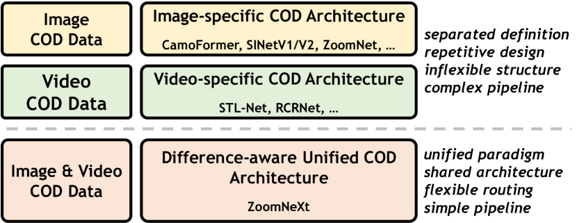
Figure 1: The main purpose of our proposed framework. The static image or video clip containing camouflaged objects can be fed into our network to yield accurate masks using the same architecture. The proposed framework, founded on the flexible routing mechanism, unifies and simplifies the processing pipeline of image and video COD tasks. Specifically, feature propagation inside multiple-scale pyramids with different information granularities ensures the accurate capture of imperceptible objects. Furthermore, the difference-aware adaptive routing mechanism empowers the proposed method with temporal conditional interaction capability only for video data, which provides a solid foundation for perceiving camouflaged objects within both image and video data.

Recently, numerous deep learning-based methods have been proposed and achieved significant progress. Nevertheless, they still struggle to accurately and reliably detect camouflaged objects, due to the visual insignificance of camouflaged objects, and high diversity in scale, appearance and occlusion. By observing our experiments, it is found that the current COD detectors are susceptible to distractors from background surroundings. Thus it is difficult to excavate discriminative and subtle semantic cues for camouflaged objects, resulting in the inability to clearly segment the camouflaged objects from the chaotic background and the predictions of some uncertain (low-confidence) regions. In addition, recent works [11, 12, 13] have attempted to introduce temporal motion cues of objects to further expand the information dimension of the COD task. However, as shown in Fig. 1, the existing best solutions for image [14, 1, 15] and video [13] COD tasks have different information emphases (i.e., the appearance information of static images and the motion information of videos), resulting in incompatibility in architecture design and feature pipeline between the two types of tasks. Taking these into mind, in this paper, we summarize the COD issue into three aspects: 1) How to accurately locate camouflaged objects under conditions of inconspicuous appearance and various scales? 2) How to design a unified framework that is compatible with both image and video feature processing pipelines? 3) How to suppress the obvious interference from the background and infer camouflaged objects more reliably? Intuitively, to accurately find the vague or camouflaged objects in the scene, humans may try to refer to and compare the changes in the shape or appearance at different scales by zooming in and out the image or video. This specific behavior pattern of human beings motivates us to identify camouflaged objects by mimicking the zooming in and out strategy.

With this inspiration, in this paper, we propose a unified collaborative pyramid network, named ZoomNeXt, which significantly improves the existing camouflaged object detection performance for the image and video COD tasks.

Firstly, for accurate object location, we employ scale space theory [16, 17, 18] to imitate zooming in and out strategy. Specifically, we design two key modules, i.e., the multi-head scale integration unit (MHSIU) and the rich granularity perception unit (RGPU). For the camouflaged object of interest, our model extracts discriminative features at different “zoom” scales using the triplet architecture, then adopts MHSIUs to screen and aggregate scale-specific features, and utilizes RGPUs to further reorganize and enhance mixed-scale features. The difference-aware adaptive routing mechanism of the module RGPU can also make full use of the inter-frame motion information to capture camouflaged objects in the video. This flexible data-aware architecture design seamlessly unifies the processing pipeline for static images and video clips into a single convolutional model. Thus, our model is able to mine the accurate and subtle semantic clues between objects and backgrounds under mixed scales and diverse scenes, and produce accurate predictions. Besides, the shared weight strategy used in the proposed method achieves a good balance of efficiency and effectiveness.

Secondly, the last aspect is related to reliable prediction in complex scenarios. Although the object is accurately located, the indistinguishable texture and background will easily bring negative effects to the model learning, e.g. predicting uncertain/ambiguity regions, which greatly reduces the detection performance and cannot be ignored. This can be seen in Fig. 9 (Row 3 and 4) and Fig. 10. To this end, we design a uncertainty awareness loss (UAL) to guide the model training, which is only based on the prior knowledge that a good COD prediction should have a clear polarization trend. Its GT-independent characteristic makes it suitable for enhancing the GT-based BCE loss. This targeted enhancement strategy can force the network to optimize the prediction of the uncertain regions during the training process, enabling our ZoomNeXt to distinguish the uncertain regions and segment the camouflaged objects reliably.

Our contributions can be summarized as follows:

1. For the COD task, we propose ZoomNeXt, which can credibly capture the objects in complex scenes by characterizing and unifying the scale-specific appearance features at different “zoom” scales and the purposeful optimization strategy.

2. To obtain the discriminative feature representation of camouflaged objects, we design MHSIUs and RGPUs to distill, aggregate and strengthen the scale-specific and subtle semantic representation for accurate COD.

3. Through a carefully-designed difference-aware adaptive routing mechanism, our unified conditional architecture seamlessly combines the image and video feature pipelines, enhancing scalability and flexibility.

4. We propose a simple yet effective optimization enhancement strategy, UAL, which can significantly suppress the uncertainty and interference from the background without increasing extra parameters.

5. Without bells and whistles, our model greatly surpasses the recent 30 state-of-the-art methods on four image and two video COD data benchmarks, respectively.

A preliminary version of this work was published in [15]. In this paper, we extend our conference version in the following aspects. First, we explore the video COD task. We extend the targeted task from the single image COD task to image and video COD tasks. Second, we improve image-specific ZoomNet to image-video unified ZoomNeXt. We extend the original static image COD framework to enable further compatibility with the new auxiliary video-related temporal cues. Third, we improve the performance of our method by introducing more structural extensions, i.e., multi-head scale integration unit and rich granularity perception unit. They make our approach superior not only to the conference version, but even to several recent cutting-edge competitors. Fourth, we also introduce and discuss more recently published algorithms for image and video tasks so as to track recent developments in the field and make fair and reasonable comparisons. Last but not least, we provide more analytical experiments and visualization to further study the effectiveness and show the characteristics of the provided components in our method including the MHSIU, RGPU, and GT-free loss function UAL, which helps to better understand their behavior.

2 Related Work

2.1 Camouflaged Object

The study of camouflage has a long history in biology. This behavior of creatures in nature can be regarded as the result of natural selection and adaptation. In fact, in human life and other parts of society, it also has a profound impact, e.g., arts, popular culture, and design. More details can be found in [19]. In the field of computer vision, research on camouflaged objects is often associated with salient object detection (SOD) [20, 21], which mainly deals with those salient and easily observed objects in the scene. In general, saliency models are designed for the general observation paradigm (i.e., finding visually prominent objects). They are not suitable for the specific observation (i.e., finding concealed objects). Therefore, it is necessary to establish models based on the essential requirements and specific data of the task to learn the special knowledge.

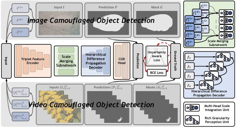
Figure 2: Overall framework of the proposed ZoomNeXt. The shared triplet feature encoder is used to extract multi-level features corresponding to different input “zoom” scales. At different levels of the scale merging subnetwork, MHSIUs are adopted to screen and aggregate the critical cues from different scales. Then the fused features are gradually integrated through the top-down up-sampling path in the hierarchical difference propagation decoder. RGPUs further enhance the feature discrimination by constructing a multi-path structure inside the features. Finally, the probability map of the camouflaged object corresponding to the input image or frame can be obtained. In the training stage, the binary cross entropy and the proposed uncertainty awareness loss are used as the loss function.

2.2 Camouflaged Object Detection (COD)

Different from the traditional SOD [22, 23, 24, 25] task, the COD task pays more attention to the undetectable objects (mainly because of too small size, occlusion, concealment or self-disguise). Due to the differences in the attributes of the objects of interest, the goals of the two tasks are different. The difficulty and complexity of the COD task far exceed the SOD task due to the high similarity between the object and the environment. Although it has practical significance in both the image and video fields, the COD task is still a relatively under-explored computer vision problem.

Some valuable attempts have been made in recent years. The pioneering works [26, 27, 28] collect and release several important image COD datasets CAMO [26], COD10K [27], and NC4K [28]. And, another vanguard [13] extends the task to the video COD task and introduces a large-scale comprehensive dataset MoCA-Mask [13]. These datasets have become representative data benchmarks for the COD task nowadays and built a solid foundation for a large number of subsequent studies.

Recent works [26, 29, 28, 30, 31, 32, 33] construct the multi-task learning framework in the prediction process of camouflaged objects and introduce some auxiliary tasks like classification, edge detection, and object gradient estimation. Among them, [32] also attempts to address the intrinsic similarity of foreground and background for COD in the frequency domain. Some uncertainty-aware methods [34, 35, 36] are proposed to model and cope with the uncertainty in data annotation or COD data itself. In the other methods [37, 38], contextual feature learning also plays an important role. And [39] introduces an explicit coarse-to-fine detection and iterative refinement strategy to refine the segmentation effect. Compared to convolutional neural networks, the vision transformer can encode global contextual information more effectively and also change the way existing methods [14, 40, 41, 42, 43, 13] perceive contextual information. Specifically, [14, 43] are based on the strategy of dividing and merging foreground and background to accurately distinguish highly similar foreground and background. [13] utilizes the multi-scale correlation aggregation and the spatiotemporal transformer to construct short-term and long-term information interactions, and optimize temporal segmentation. [40] aims to enhance locality modeling of the transformer-based model and the feature aggregation in decoders, while [41] preserves detailed clues through the high-resolution iterative feedback design. In addition, there are also a number of bio-inspired methods, such as [27, 1, 44]. They capture camouflaged objects by imitating the behavior process of hunters or changing the viewpoint of the scene.

Although our method can also be attributed to the last category, ours is different from the above methods. Our method simulates the behavior of humans to understand complex images by zooming in and out strategy. The proposed method explores the scale-specific and imperceptible semantic features under the mixed scales for accurate predictions, with the supervision of BCE and our proposed UAL. At the same time, through the adaptive perception ability of the temporal difference, the proposed method also harmonizes both image and video data in a single framework. Accordingly, our method achieves a more comprehensive understanding of the diverse scene, and accurately and robustly segments the camouflaged objects from the complex background.

2.3 Conditional Computation

Conditional computation [45] refers to a series of carefully constructed algorithms in which each input sample actually uses only a subset of feature processing nodes. It can further reduce computation, latency, or power on average, and increase model capacity without a proportional increase in computation. As argued in [45], sparse activations and multiplicative connections may be useful ingredients of conditional computation. Over the past few years, it has become an important solution to the time-consuming and computationally expensive training and inference of deep learning models. Specifically, as a typical paradigm, the mixture of experts (MoE) technique [46] based on sparse selection has shown great potential on a variety of different types of tasks, including language modeling and machine translation [47], multi-task learning [48], image classification [49, 50], and vision-language model [51]. Existing methods mainly rely on MoE and gating strategies to realize dynamic routing of feature flow nodes, and focus on the distinction between different samples of homogeneous data. In the proposed scheme, we propose a new form of conditional computation for differentiated processing of image and video data. Specifically, we construct adaptive video-specific bypasses using the inter-frame difference in video, which automatically ”ignores” static images for good task compatibility.

2.4 Scale Space Integration

The scale-space theory aims to promote an optimal understanding of image structure, which is an extremely effective and theoretically sound framework for addressing naturally occurring scale variations. Its ideas have been widely used in computer vision, including the image pyramid [52] and the feature pyramid [53]. Due to the structural and semantic differences at different scales, the corresponding features play different roles. However, the commonly-used inverted pyramid-like feature extraction structures [54, 55, 56] often cause the feature representation to lose too much texture and appearance details, which are unfavorable for dense prediction tasks [57, 58] that emphasize the integrity of regions and edges. Thus, some recent CNN-based COD methods [27, 38, 37, 29] and SOD methods [59, 60, 61, 62, 63, 64, 65] explore the combination strategy of inter-layer features to enhance the feature representation. These bring some positive gains for accurate localization and segmentation of objects. However, for the COD task, the existing approaches overlook the performance bottleneck caused by the ambiguity of the structural information of the data itself which makes it difficult to be fully perceived at a single scale. Different from them, we mimic the zoom strategy to synchronously consider differentiated relationships between objects and background at multiple scales, thereby fully perceiving the camouflaged objects and confusing scenes. Besides, we also further explore the fine-grained feature scale space between channels.

3 Method

In this section, we first elaborate on the overall architecture of the proposed method, and then present the details of each module and the uncertainty awareness loss function.

3.1 Overall Architecture

Preliminaries Let $\mathbf{I}\in\mathbb{R}^{3\times H\times W}$ and $\{\mathbf{I}_{t}\in\mathbb{R}^{3\times H\times W}\}^{T}_{t=1}$ be the input static image and the input video clip with $T$ frames of the network, where $3$ is the number of color channels and $H,W$ are the height and width. Our network is to generate a gray-scale map $\mathbf{P}$ or clip $\{\mathbf{P}_{t}\}^{T}_{t=1}$ with values ranging from 0 to 1, which reflects the probability that each location may be part of the camouflaged object.

Zooming Strategy The overall architecture of the proposed method is illustrated in Fig. 2. Inspired by the zooming strategy from human beings when observing confusing scenes, we argue that different zoom scales often contain their specific information. Aggregating the differentiated information on different scales will benefit exploring the inconspicuous yet valuable clues from confusing scenarios, thus facilitating COD. To implement it, intuitively, we resort to the image pyramid. Specifically, we customize an image pyramid based on the single scale input to identify the camouflaged objects. The scales are divided into a main scale (i.e. the input scale) and two auxiliary scales. The latter is obtained by re-scaling the input to imitate the operation of zooming in and out.

Feature Processing We utilize the shared triplet feature encoder to extract features on different scales and feed them to the scale merging subnetwork. To integrate these features that contain rich scale-specific information, we design a series of multi-head scale integration units (MHSIUs) based on the attention-aware filtering mechanism. Thus, these auxiliary scales are integrated into the main scale, i.e., information aggregation of “zoom in and out” operation. This will largely enhance the model to distill critical and informative semantic cues for capturing difficult-to-detect camouflaged objects. After that, we construct rich granularity perception units (RGPUs) to gradually integrate multi-level features in a top-down manner to enhance the mixed-scale feature representation. It further increases the receptive field range and diversifies feature representation within the module. The captured fine-grained and mixed-scale clues promote the model to accurately segment the camouflaged objects in the chaotic scenes.

Loss Improvement To overcome the uncertainty in the prediction caused by the inherent complexity of the data, we design an uncertainty awareness loss (UAL) to assist the BCE loss, enabling the model to distinguish these uncertain regions and produce an accurate and reliable prediction.

3.2 Triplet Feature Encoder

We start by extracting deep features through a shared triplet feature encoder for the group-wise inputs, which consists of a feature extraction network and a channel compression network. The feature extraction network is constituted by the commonly-used ResNet [66], EfficientNet [67], or PVTv2 [68] that removes the classification head. And the channel compression network is cascaded to further optimize computation and obtain a more compact feature. For the trade-off between efficiency and effectiveness, the main scale and the two auxiliary scales are empirically set to $1.0\times$, $1.5\times$ and $0.5\times$. And, three sets of 64-channel feature maps corresponding to three input scales are produced by these structures, i.e., $\{f^{k}_{i}\}_{i=1}^{5},\,k\in\{0.5,1.0,1.5\}$. Next, these features are fed successively to the multi-head scale merging subnetwork and the hierarchical difference propagation decoder for subsequent processing.

Figure 3: Illustration of the multi-head scale integration unit.

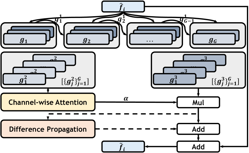
Figure 4: Rich granularity perception unit. Group-wise interaction and channel-wise modulation are used to explore the discriminative and valuable semantics from different channels. Note that each group of features is executed sequentially. The latter one integrates part of the features of the previous one before the feature transformation.

3.3 Scale Merging Subnetwork

We design an attention-based multi-head scale integration unit (MHSIU) to screen (weight) and combine scale-specific information, as shown in Fig. 3. Several such units make up the scale merging subnetwork. Through filtering and aggregation, the expression of different scales is self-adaptively highlighted. The details of this component are described next.

Scale Alignment Before scale integration, the features $f^{1.5}_{i}$ and $f^{0.5}_{i}$ are first resized to be consistent resolution with the main scale feature $f^{1.0}_{i}$. Specifically, for $f^{1.5}_{i}$, we use a hybrid structure of “max-pooling + average-pooling” to down-sample it, which helps to preserve the effective and diverse responses for camouflaged objects in high-resolution features. For $f^{0.5}_{i}$, we directly up-sample it by the bi-linear interpolation. Then, these features are fed into the “attention generator”.

Multi-Head Spatial Interaction Unlike the form of spatial attention in our conference version [15] that relies heavily on a single pattern, here we perform parallel independent transformations on $M$ groups of feature maps, which is inspired by the structure of the multi-head paradigm in Transformer [69]. This design helps extend the model’s ability to mine multiple fine-grained spatial attention patterns in parallel and diversify the representation of the feature space. Specifically, several three-channel feature maps are calculated through a series of convolutional layers. After the cascaded softmax activation layer in each attention group, the attention map $A^{k}_{m}$ corresponding to each scale can be obtained from these groups and used as respective weights for the final integration, where scale group index $k\in\{1,2,3\}$ and attention group index $m\in\{1,2,\dots,M\}$. The process is formulated as:

$$\begin{split}F_{i}&=\left[\mathcal{U}(f^{0.5}_{i}),f^{1.0}_{i},\mathcal{D}(f^{1.5}_{i})\right],\\ \hat{F}_{i}&=\{\texttt{trans}(F_{i},\phi^{m})\}_{m=1}^{M},\\ A_{i}&=\{\texttt{softmax}(\hat{F}_{i,m})\}_{m=1}^{M},\\ \tilde{F}_{i}&=\{\texttt{trans}(F_{i},\gamma^{m})\}_{m=1}^{M},\\ f_{i}&=\{A^{1}_{i,m}\cdot\tilde{F}^{1}_{i,m}+A^{2}_{i,m}\cdot\tilde{F}^{2}_{i,m}+A^{3}_{i,m}\cdot\tilde{F}^{3}_{i,m}\}_{m=1}^{M},\end{split}$$ (1)

where $\left[\star\right]$ represents the concatenation operation. $\mathcal{U}$ and $\mathcal{D}$ refer to the bi-linear interpolation and hybrid adaptive pooling operations mentioned above, respectively. $\texttt{trans}(\star,\phi)$ and $\texttt{trans}(\star,\gamma)$ indicate the several simple linear transformation layers in the attention generator, and $\phi$ and $\gamma$ mean the parameters of these layers. Note that some linear, normalization and activation layers before and after the sampling operation are not shown in Equ. 1 and Fig. 3 for simplicity. And features enhanced in different groups are concatenated along the channel dimension and fed into a decoder for further processing. These designs aim to adaptively and selectively aggregate the scale-specific information to explore subtle but critical semantic cues at different scales, boosting the feature representation.

3.4 Hierarchical Difference Propagation Decoder

1

Input: $\{g_{j}\}_{j=1}^{G}$: feature groups; $G\geq 2$: the number of groups; $\texttt{CBR}_{C_{o}\times C_{i}}$: “$3\times 3$Conv-BN-ReLU” units with input and output channel numbers of $C_{i}$ and $C_{o}$; split and concat: channel-wise splitting and concatenating;

Output: $\{{g^{\prime}}^{2}_{j}\}_{j=1}^{G}$: the feature set for generating the modulation vector $\alpha$; $\{{g^{\prime}}^{3}_{j}\}_{j=1}^{G}$: the feature set used to be modulated and generate the final output of the RGPU;

2 for $i\leftarrow 1,G$ do

3       if  $i=1$  then /* Group $1$ */

4             $f\leftarrow\texttt{CBR}^{i}_{3C\times C}(g_{i})$;

5             ${g^{\prime}}^{1}_{i},{g^{\prime}}^{2}_{i},{g^{\prime}}^{3}_{i}\leftarrow\texttt{split}(f)$;

6             ${g^{\prime}}^{1}_{prev}\leftarrow{g^{\prime}}^{1}_{i}$;

7            

8       else if  $i=G$  then /* Group $G$ */

9             $f\leftarrow\texttt{CBR}^{i}_{2C\times 2C}(\texttt{concat}(g_{i},{g^{\prime}}^{1}_{prev}))$;

10             ${g^{\prime}}^{2}_{i},{g^{\prime}}^{3}_{i}\leftarrow\texttt{split}(f)$;

11            

12       else  /* Group $i$, $1<i<G$ */

13             $f\leftarrow\texttt{CBR}^{i}_{3C\times 2C}(\texttt{concat}(g_{i},{g^{\prime}}^{1}_{prev}))$;

14             ${g^{\prime}}^{1}_{i},{g^{\prime}}^{2}_{i},{g^{\prime}}^{3}_{i}\leftarrow\texttt{split}(f)$;

15             ${g^{\prime}}^{1}_{prev}\leftarrow{g^{\prime}}^{1}_{i}$;

16            

17       end if

18      

19 end for

Algorithm 1 The iteration process in the RGPU.

After MHSIUs, the auxiliary-scale information is integrated into the main-scale branch. Similar to the multi-scale case, different channels also contain differentiated semantics. Thus, it is necessary to excavate valuable clues contained in different channels. To this end, we design the rich granularity perception unit (RGPU) to conduct information interaction and feature refinement between channels, which strengthen features from coarse-grained group-wise iteration to fine-grained channel-wise modulation in the decoder, as depicted in Fig. 4.

Input The input $\hat{f}_{i}$ of the RGPU_i contains the multi-scale fused feature $f_{i}$ from the MHSIU_i and the feature $\tilde{f}_{i+1}$ from the RGPU_i+1 as $\hat{f}_{i}=f_{i}+\mathcal{U}(\tilde{f}_{i+1})$.

Group-wise Iteration We adopt $1\times 1$ convolution to extend the channel number of feature map $\hat{f}_{i}$. The features are then divided into $G$ groups $\{g_{j}\}_{j=1}^{G}$ along the channel dimension. Feature interaction between groups is carried out in an iterative manner. Specifically, the first group $g_{1}$ is split into three feature sets $\{{g^{\prime}}_{1}^{k}\}_{k=1}^{3}$ after a convolution block. Among them, the ${g^{\prime}}_{1}^{1}$ is adopted for information exchange with the next group, and the other two are used for channel-wise modulation. In the $j^{th}$ ($1<j<G$) group, the feature $g_{j}$ is concatenated with the feature ${g^{\prime}}_{j-1}^{1}$ from the previous group along the channel, followed by a convolution block and a split operation, which similarly divides this feature group into three feature sets. It is noted that the output of the group $G$ with the similar input form to the previous groups only contains ${g^{\prime}}_{G}^{2}$ and ${g^{\prime}}_{G}^{3}$. Such an iterative mixing strategy strives to learn the critical clues from different channels and obtain a powerful feature representation. The iteration structure of feature groups in RGPU is actually equivalent to an integrated multi-path kernel pyramid structure with partial parameter sharing. Such a design further enriches the ability to explore diverse visual cues, thereby helping to better perceive objects and refine predictions. The iteration processing is also listed in Alg. 1.

Channel-wise Modulation The features $[\{{g^{\prime}}_{j}^{2}\}_{j=1}^{G}]$ are concatenated and converted into the feature modulation vector $\mathbf{\alpha}$ by a small convolutional network, which is employed to weight another concatenated feature as $\bar{f}_{i}=\alpha\cdot[\{{g^{\prime}}_{j}^{3}\}_{j=1}^{G}]$.

Difference-based Conditional Computation Because the inter-frame difference can directly reflect the temporal motion cues of the camouflaged object in the video, we design the difference-aware adaptive routing mechanism to realize the video-specific inter-frame information propagation and seamlessly unify the image and video COD tasks. Specifically, the features from the group-wise iteration and the channel-wise modulation first utilize the temporal shift operation shift to obtain the difference representation $X=\texttt{shift}(\bar{f}_{i})-\bar{f}_{i}$ between adjacent frames. To enhance the motion cues of the object of interest between frames, the intra-frame self-attention is performed as $Z=XW_{V}\texttt{softmax}(\frac{(XW_{K})^{\top}XW_{Q}}{\sqrt{HW}})$. And these cues are further diffused among video clips by the following convolutional layers performed in the time dimension and added to the original feature $\bar{f}_{i}$. For the static image, this pipeline outputs an all-zero tensor, thus maintaining the original features.

Output The output feature of the RGPU can be obtained by the stacked activation, normalization and convolutional layers, which are defined as: $\tilde{f}_{i}=\texttt{fuse}(\hat{f}_{i}+\bar{f}_{i})$. Based on cascaded RGPUs and several stacked convolutional layers, a single-channel logits map is obtained. The final confidence map $\mathbf{P}$ or map group $\{\mathbf{P}_{t}\}^{T}_{t=1}$ that highlights the camouflaged objects is then generated by a sigmoid function.

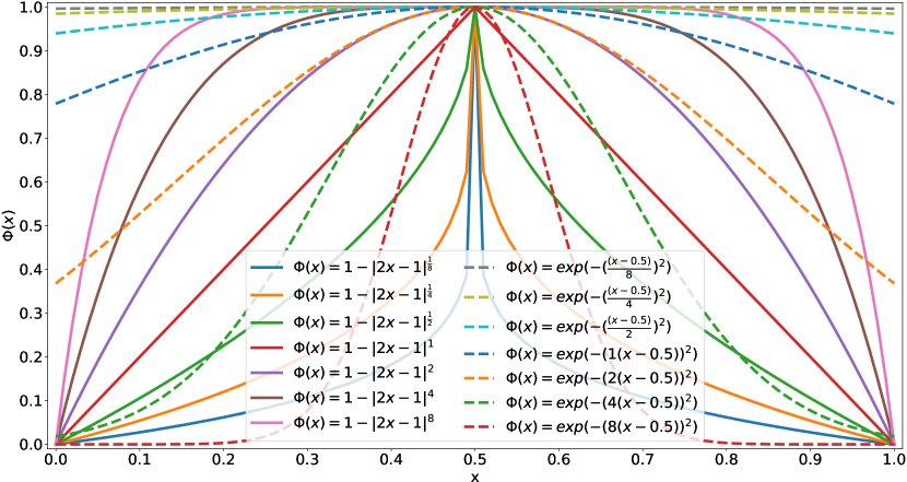
Figure 5: Curves of different forms of the proposed UAL.

TABLE I: Comparisons of different methods based on different backbones on static image COD datasets. ^⋆: Using more datasets. The best three results are highlighted in red, green and blue.

		CAMO					CHAMELEON					COD10K					NC4K
Model	Backbone	Sm $\uparrow$	F${}^{\omega}_{\beta}$ $\uparrow$	MAE $\downarrow$	Fβ $\uparrow$	Em $\uparrow$	Sm $\uparrow$	F${}^{\omega}_{\beta}$ $\uparrow$	MAE $\downarrow$	Fβ $\uparrow$	Em $\uparrow$	Sm $\uparrow$	F${}^{\omega}_{\beta}$ $\uparrow$	MAE $\downarrow$	Fβ $\uparrow$	Em $\uparrow$	Sm $\uparrow$	F${}^{\omega}_{\beta}$ $\uparrow$	MAE $\downarrow$	Fβ $\uparrow$	Em $\uparrow$
Convolutional Neural Network based Methods
SINet20 [27]	ResNet-50	0.745	0.644	0.091	0.702	0.829	0.872	0.806	0.034	0.827	0.946	0.776	0.631	0.043	0.679	0.874	0.808	0.723	0.058	0.769	0.883
SLSR21 [28]	ResNet-50	0.787	0.696	0.080	0.744	0.854	0.890	0.822	0.030	0.841	0.948	0.804	0.673	0.037	0.715	0.892	0.840	0.765	0.048	0.804	0.907
MGL-R21 [29]	ResNet-50	0.775	0.673	0.088	0.726	0.842	0.893	0.812	0.030	0.834	0.941	0.814	0.666	0.035	0.710	0.890	0.833	0.739	0.053	0.782	0.893
PFNet21 [37]	ResNet-50	0.782	0.695	0.085	0.746	0.855	0.882	0.810	0.033	0.828	0.945	0.800	0.660	0.040	0.701	0.890	0.829	0.745	0.053	0.784	0.898
UJSC${}_{\star}^{21}$ [34]	ResNet-50	0.800	0.728	0.073	0.772	0.873	0.891	0.833	0.030	0.848	0.955	0.809	0.684	0.035	0.721	0.891	0.842	0.771	0.046	0.806	0.907
C2FNet21 [38]	ResNet-50	0.796	0.719	0.080	0.762	0.864	0.888	0.828	0.032	0.844	0.946	0.813	0.686	0.036	0.723	0.900	0.838	0.762	0.049	0.794	0.904
UGTR21 [35]	ResNet-50	0.784	0.684	0.086	0.735	0.851	0.887	0.794	0.031	0.819	0.940	0.817	0.666	0.036	0.711	0.890	0.839	0.746	0.052	0.787	0.899
ZoomNet22 [15]	ResNet-50	0.820	0.752	0.066	0.794	0.892	0.902	0.845	0.023	0.864	0.958	0.838	0.729	0.029	0.766	0.911	0.853	0.784	0.043	0.818	0.912
SINetV221 [1]	Res2Net-50	0.820	0.743	0.070	0.782	0.895	0.888	0.816	0.030	0.835	0.961	0.815	0.680	0.037	0.718	0.906	0.847	0.770	0.048	0.805	0.914
BSA-Net22 [30]	Res2Net-50	0.794	0.717	0.079	0.763	0.867	0.895	0.841	0.027	0.858	0.957	0.818	0.699	0.034	0.738	0.901	0.842	0.771	0.048	0.808	0.907
BGNet22 [31]	Res2Net-50	0.812	0.749	0.073	0.789	0.882	0.901	0.851	0.027	0.860	0.954	0.831	0.722	0.033	0.753	0.911	0.851	0.788	0.044	0.820	0.916
SegMaR22 [39]	ResNet-50	0.815	0.753	0.071	0.795	0.884	0.906	0.860	0.025	0.872	0.959	0.833	0.724	0.034	0.757	0.906	0.841	0.781	0.046	0.821	0.907
CamoFormer-R22 [14]	ResNet-50	0.817	0.752	0.067	0.792	0.885	0.898	0.847	0.025	0.867	0.956	0.838	0.724	0.029	0.753	0.930	0.855	0.788	0.042	0.821	0.914
FEDER23 [32]	ResNet-50	0.802	0.738	0.071	0.781	0.873	0.887	0.835	0.030	0.851	0.954	0.822	0.716	0.032	0.751	0.905	0.847	0.789	0.044	0.824	0.915
DGNet23 [33]	EfficientNet-B4	0.838	0.768	0.057	0.805	0.914	0.890	0.816	0.029	0.834	0.956	0.822	0.692	0.033	0.727	0.911	0.857	0.783	0.042	0.813	0.922
Ours23	ResNet-50	0.833	0.774	0.065	0.813	0.891	0.908	0.858	0.021	0.874	0.963	0.861	0.768	0.026	0.801	0.925	0.874	0.816	0.037	0.846	0.928
Ours23	EfficientNet-B4	0.867	0.824	0.046	0.852	0.925	0.911	0.865	0.020	0.879	0.964	0.875	0.797	0.021	0.824	0.941	0.884	0.837	0.032	0.862	0.939
Vision Transoformer based Methods
CamoFormer-P22 [14]	PVTv2-B4	0.872	0.831	0.046	0.854	0.938	0.910	0.865	0.022	0.882	0.966	0.869	0.786	0.023	0.811	0.939	0.892	0.847	0.030	0.868	0.946
FSPNet23 [40]	ViT-B16	0.856	0.799	0.050	0.831	0.928	0.908	0.851	0.023	0.867	0.965	0.851	0.735	0.026	0.769	0.930	0.878	0.816	0.035	0.843	0.937
HitNet23 [41]	PVTv2-B2	0.849	0.809	0.055	0.831	0.910	0.921	0.897	0.019	0.900	0.972	0.871	0.806	0.023	0.823	0.938	0.875	0.834	0.037	0.854	0.929
MSCAF-Net23 [42]	PVTv2-B2	0.873	0.828	0.046	0.852	0.937	0.912	0.865	0.022	0.876	0.970	0.865	0.775	0.024	0.798	0.936	0.887	0.838	0.032	0.860	0.942
SARNet23 [43]	PVTv2-B3	0.874	0.844	0.046	0.866	0.935	0.933	0.909	0.017	0.915	0.978	0.885	0.820	0.021	0.839	0.947	0.889	0.851	0.032	0.872	0.940
Ours23	PVTv2-B2	0.874	0.839	0.047	0.863	0.931	0.922	0.884	0.017	0.896	0.970	0.887	0.818	0.019	0.841	0.948	0.892	0.852	0.030	0.874	0.943
Ours23	PVTv2-B3	0.885	0.854	0.042	0.872	0.942	0.927	0.898	0.017	0.905	0.977	0.895	0.829	0.018	0.848	0.952	0.900	0.861	0.028	0.880	0.949
Ours23	PVTv2-B4	0.888	0.859	0.040	0.878	0.943	0.925	0.897	0.016	0.906	0.973	0.898	0.838	0.017	0.857	0.955	0.900	0.865	0.028	0.884	0.949
Ours23	PVTv2-B5	0.889	0.857	0.041	0.875	0.945	0.924	0.885	0.018	0.896	0.975	0.898	0.827	0.018	0.848	0.956	0.903	0.863	0.028	0.884	0.951

TABLE II: Comparisons of different methods on video COD datasets. “T” represents the number of frames in the video clip. “T=1” is the model without temporal difference, where the dynamic routing is not activated. “T=5” is our final model for the video COD task due to its better performance. The best three results are highlighted in red, green and blue.

		CAD							MoCA-Mask-TE
Model	Backbone	S${}_{m}~{}\uparrow$	F${}^{\omega}_{\beta}~{}\uparrow$	MAE$~{}\downarrow$	F${}_{\beta}~{}\uparrow$	E${}_{m}~{}\uparrow$	mDice$~{}\uparrow$	mIoU$~{}\uparrow$	S${}_{m}~{}\uparrow$	F${}^{\omega}_{\beta}~{}\uparrow$	MAE$~{}\downarrow$	F${}_{\beta}~{}\uparrow$	E${}_{m}~{}\uparrow$	mDice$~{}\uparrow$	mIoU$~{}\uparrow$
EGNet19 [70]	ResNet-50	0.619	0.298	0.044	0.350	0.666	0.324	0.243	0.547	0.110	0.035	0.136	0.574	0.143	0.096
BASNet19 [71]	ResNet-50	0.639	0.349	0.054	0.394	0.773	0.393	0.293	0.561	0.154	0.042	0.173	0.598	0.190	0.137
CPD19 [72]	ResNet-50	0.622	0.289	0.049	0.357	0.667	0.330	0.239	0.561	0.121	0.041	0.152	0.613	0.162	0.113
PraNet20 [4]	ResNet-50	0.629	0.352	0.042	0.397	0.763	0.378	0.290	0.614	0.266	0.030	0.296	0.674	0.311	0.234
SINet20 [27]	ResNet-50	0.636	0.346	0.041	0.395	0.775	0.381	0.283	0.598	0.231	0.028	0.256	0.699	0.277	0.202
SINet-V221 [1]	Res2Net-50	0.653	0.382	0.039	0.432	0.762	0.413	0.318	0.588	0.204	0.031	0.229	0.642	0.245	0.180
PNS-Net21 [73]	ResNet-50	0.655	0.325	0.048	0.417	0.673	0.384	0.290	0.526	0.059	0.035	0.084	0.530	0.084	0.054
RCRNet19 [74]	ResNet-50	0.627	0.287	0.048	0.328	0.666	0.309	0.229	0.555	0.138	0.033	0.159	0.527	0.171	0.116
MG21 [75]	Res2Net-50	0.594	0.336	0.059	0.375	0.692	0.368	0.268	0.530	0.168	0.067	0.195	0.561	0.181	0.127
STL-Net-LT22 [13]	PVTv2-B5	0.696	0.481	0.030	0.524	0.845	0.493	0.402	0.631	0.311	0.027	0.331	0.759	0.360	0.272
STL-Net-ST22 [13]	PVTv2-B5	0.696	0.471	0.031	0.515	0.827	0.484	0.392	0.637	0.304	0.027	0.328	0.734	0.356	0.271
Ours23 (T=1)	PVTv2-B5	0.721	0.525	0.024	0.567	0.759	0.523	0.436	0.690	0.395	0.017	0.424	0.702	0.420	0.353
Ours23 (T=3)	PVTv2-B5	0.741	0.565	0.021	0.598	0.849	0.571	0.487	0.703	0.425	0.010	0.444	0.717	0.446	0.378
Ours23 (T=5)	PVTv2-B5	0.757	0.593	0.020	0.631	0.865	0.599	0.510	0.734	0.476	0.010	0.497	0.736	0.497	0.422
Ours23 (T=7)	PVTv2-B5	0.751	0.583	0.020	0.618	0.837	0.591	0.505	0.706	0.428	0.011	0.444	0.717	0.446	0.382

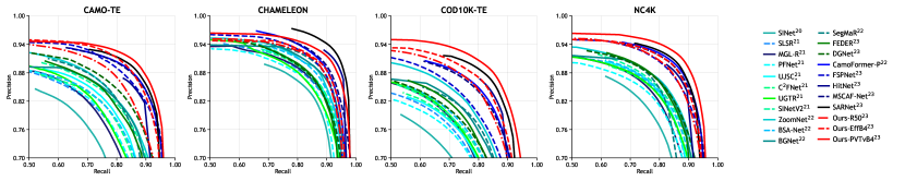
(a) PR curves.

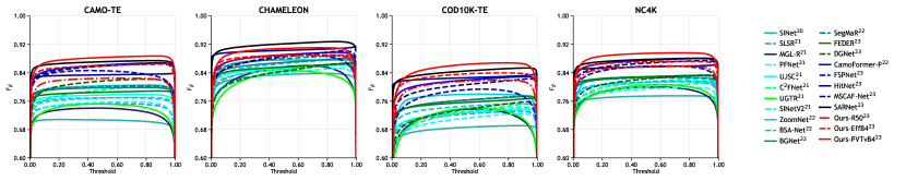
(b) $F_{\beta}$ curves.

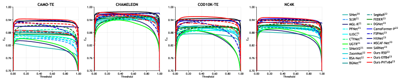
(c) $E_{m}$ curves.

Figure 6: PR, $F_{\beta}$ and $E_{m}$ curves of the proposed model and recent SOTA algorithms over four COD datasets.

3.5 Loss Functions

Binary Cross Entropy Loss (BCE) The BCE loss function is widely used in various binary image segmentation tasks and its mathematical form is:

$$\begin{split}l_{BCE}^{i,j}=-\mathbf{g}_{i,j}\log\mathbf{p}_{i,j}-(1-\mathbf{g}_{i,j})\log(1-\mathbf{p}_{i,j}),\end{split}$$ (2)

where $\mathbf{g}_{i,j}\in\{0,1\}$ and $\mathbf{p}_{i,j}\in[0,1]$ denote the ground truth and the predicted value at position $(i,j)$, respectively. As shown in Fig. 9, due to the complexity of the COD data, if trained only under the BCE, the model produces serious ambiguity and uncertainty in the prediction and fails to accurately capture objects, of which both will reduce the reliability of COD.

Uncertainty Awareness Loss (UAL) To force the model to enhance “confidence” in decision-making and increase the penalty for fuzzy prediction, we design a strong constraint as the auxiliary of the BCE, i.e., the uncertainty awareness loss (UAL). In the final probability map of the camouflaged object, the pixel value range is $[0,1]$, where $0$ means the pixel belongs to the background, and $1$ means it belongs to the camouflaged object. Therefore, the closer the predicted value is to $0.5$, the more uncertain the determination about the property of the pixel is. To optimize it, a direct way is to use ambiguity as the supplementary loss for these difficult samples. To this end, we first need to define the ambiguity measure of the pixel $x$, which maximizes at $x=0.5$ and minimizes at $x=0$ or $x=1$. As a loss, the function should be smooth and continuous with only a finite number of non-differentiable points. For brevity, we empirically consider two forms, $\Phi_{pow}^{\alpha}(x)=1-|2x-1|^{\alpha}$ based on the power function and $\Phi_{exp}^{\alpha}(x)=e^{-(\alpha(x-0.5))^{2}}$ based on the exponential function. Besides, inspired by the form of the weighted BCE loss, we also try to use $\omega=1+\Phi_{pow}^{2}(x)$ as the weight of BCE loss to increase the loss of hard pixels. The different forms and corresponding results are listed in Fig. 5 and Tab. VI. After massive experiments (Sec. 4.3.5), the proposed UAL is formulated as

$$\begin{split}l_{{UAL}}^{i,j}=1-\Delta_{i,j}=1-|2\mathbf{p}_{i,j}-1|^{2}.\end{split}$$ (3)

Total Loss Function Finally, the total loss function can be written as: $L=L_{BCE}+\lambda L_{{UAL}}$, where $\lambda$ is the balance coefficient. We design three adjustment strategies of $\lambda$, i.e., a fixed constant value, an increasing linear strategy, and an increasing cosine strategy in Sec. 4.3.5. From the results shown in Tab. V, we find that the increasing strategies, especially “cosine”, do achieve better performance. So, the cosine strategy is used by default.

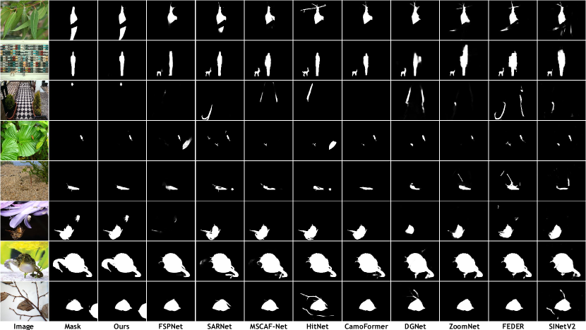
Figure 7: Visual comparisons of some recent COD methods and ours on different types of samples.

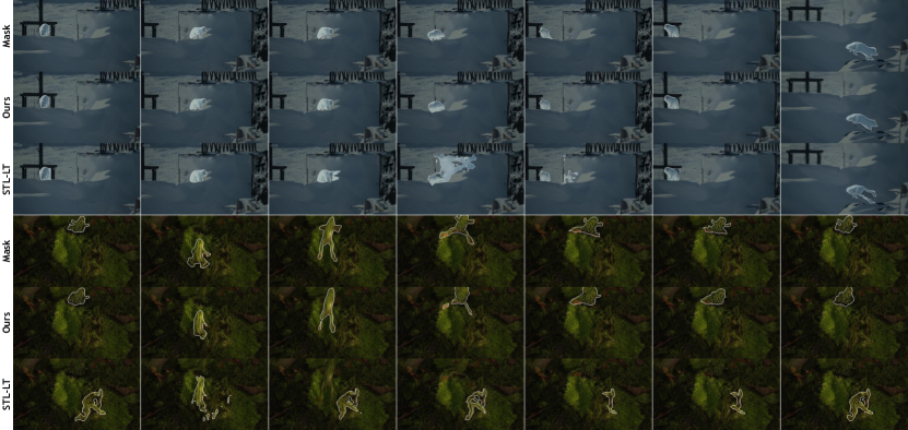
Figure 8: Visual comparisons of “Ours (T=5)” and recent best practice STL-Net-LT [13] for video COD. For better visualization, the grey-scale predictions are thresholded by 0.5 here.

4 Experiments

4.1 Experiment Setup

4.1.1 Datasets

We use four image COD datasets, CAMO [26], CHAMELEON [76], COD10K [27] and NC4K [28], and two video COD datasets, MoCA-Mask [13] and CAD [12].

Image COD CAMO consists of 1,250 camouflaged and 1,250 non-camouflaged images. CHAMELEON contains 76 hand-annotated images. COD10K includes 5,066 camouflaged, 3,000 background and 1,934 non-camouflaged images. NC4K is another large-scale COD testing dataset including 4,121 images from the Internet. Following the data partition of [27, 37, 15, 14, 33], we use all images with camouflaged objects in the experiments, in which 3,040 images from COD10K and 1,000 images from CAMO for training, and the rest ones for testing.

Video COD The recent MoCA-Mask is reorganized from the moving camouflaged animals (MoCA) dataset [11]. MoCA-Mask includes 71 sequences with 19,313 frames for training, and 16 sequences with 3,626 frames for testing, respectively. And it extends the original bounding box annotations of the MoCA dataset to finer segmentation annotations. The camouflaged animal dataset, i.e., CAD, includes 9 short video sequences in total that accompany 181 hand-labeled masks on every $5^{th}$ frame. Except for the training set containing 71 frame sequences of MoCA-Mask for training, the rest of the video sequences are used for testing as [13].

4.1.2 Evaluation Criteria

For image COD, we use eight common metrics for evaluation based on [77, 78], including S-measure [79] (S_m), weighted F-measure [80] (F${}_{\beta}^{\omega}$), mean absolute error (MAE), F-measure [81] (F_β), E-measure [82] (E_m), precision-recall curve (PR curve), F_β-threshold curve (F_β curve), and E_m-threshold curve (E_m curve). And for video COD, the seven metrics used in the recent pioneer work [13] are introduced to evaluate existing methods, including S_m, F${}_{\beta}^{\omega}$, MAE, F_β, E_m, mDice, and mIoU.

4.1.3 Implementation Details

The proposed camouflaged object detector is implemented with PyTorch [83]. And the training settings are on par with recent best practices [27, 37, 15, 33, 14, 13]. The encoder is initialized with the parameters of ResNet [66], EfficientNet [67] and PVTv2 [68] pre-trained on ImageNet, and the remaining parts are randomly initialized. The optimizer Adam with $\texttt{betas}=(0.9,0.999)$ is chosen to update the model parameters. The learning rate is initialized to 0.0001 and follows a step decay strategy. The entire model is trained for 150 epochs with a batch size of 8 in an end-to-end manner on an NVIDIA 2080Ti GPU. During training and inference, the scales of the main input and the ground truth are set to $384\times 384$. Random flipping, rotating, and color jittering are employed to augment the training data and no test-time augmentation is used in the inference phase. In addition, for a fair comparison, we follow the settings used in [13] in the video COD task, i.e., pre-training on COD10K-TR + fine-tuning on MoCA-Mask-TR.

TABLE III: Ablation study on COD10K-TE and NC4K. RGPU: Rich granularity perception unit; MHSIU: Multi-head Scale integration unit; UAL: Uncertainty awareness loss; ARG: Average relative gain.

				COD10K					NC4K
No.	Model	Param. (M)	GFLOPs	Sm $\uparrow$	F${}^{\omega}_{\beta}$ $\uparrow$	MAE $\downarrow$	Fβ $\uparrow$	Em $\uparrow$	Sm $\uparrow$	F${}^{\omega}_{\beta}$ $\uparrow$	MAE $\downarrow$	Fβ $\uparrow$	Em $\uparrow$	ARG
0	Baseline	25.216	41.000	0.826	0.677	0.035	0.724	0.903	0.850	0.756	0.049	0.800	0.912	0.00%
1.1	No.0 + RGPU ($G=2$)	25.583	47.801	0.836	0.691	0.033	0.739	0.913	0.859	0.769	0.047	0.808	0.916	$\uparrow$2.05%
1.2	No.0 + RGPU ($G=4$)	26.364	62.748	0.839	0.696	0.032	0.740	0.915	0.859	0.770	0.046	0.809	0.916	$\uparrow$2.71%
1.3	No.0 + RGPU ($G=6$)	27.145	77.694	0.843	0.705	0.031	0.749	0.914	0.863	0.778	0.045	0.816	0.919	$\uparrow$3.77%
1.4	No.0 + RGPU ($G=8$)	27.926	92.641	0.839	0.700	0.032	0.744	0.911	0.861	0.775	0.045	0.812	0.915	$\uparrow$3.10%
2.1	No.0 + SIU	26.762	152.720	0.852	0.721	0.031	0.763	0.919	0.862	0.780	0.044	0.818	0.919	$\uparrow$4.60%
2.2	No.0 + MH-SIU ($M=2$)	26.576	150.306	0.853	0.724	0.030	0.768	0.922	0.864	0.784	0.043	0.822	0.922	$\uparrow$5.41%
2.3	No.0 + MH-SIU ($M=4$)	26.530	149.100	0.856	0.728	0.029	0.770	0.923	0.870	0.789	0.043	0.825	0.924	$\uparrow$6.03%
2.4	No.0 + MH-SIU ($M=8$)	26.518	148.498	0.856	0.726	0.029	0.769	0.924	0.867	0.783	0.044	0.820	0.922	$\uparrow$5.59%
3	No.0 + RGPU ($G=6$) +MHSIU ($M=4$)	28.458	185.794	0.861	0.734	0.029	0.773	0.924	0.875	0.792	0.042	0.826	0.925	$\uparrow$6.56%
4	No.3 + UAL	28.458	185.794	0.861	0.768	0.026	0.801	0.925	0.874	0.816	0.037	0.846	0.928	$\uparrow$9.94%

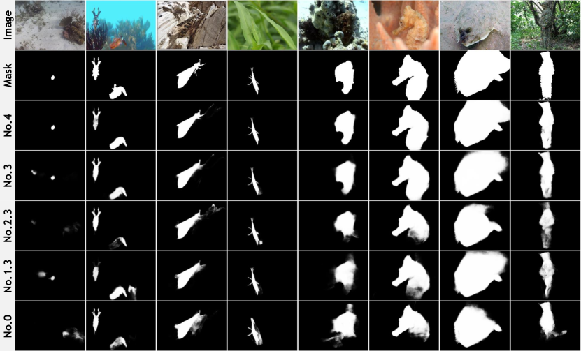
Figure 9: Visual comparisons for showing the effects of the proposed components. The names “No.x” are the same as those in Tab. III. Please zoom in to see more details.

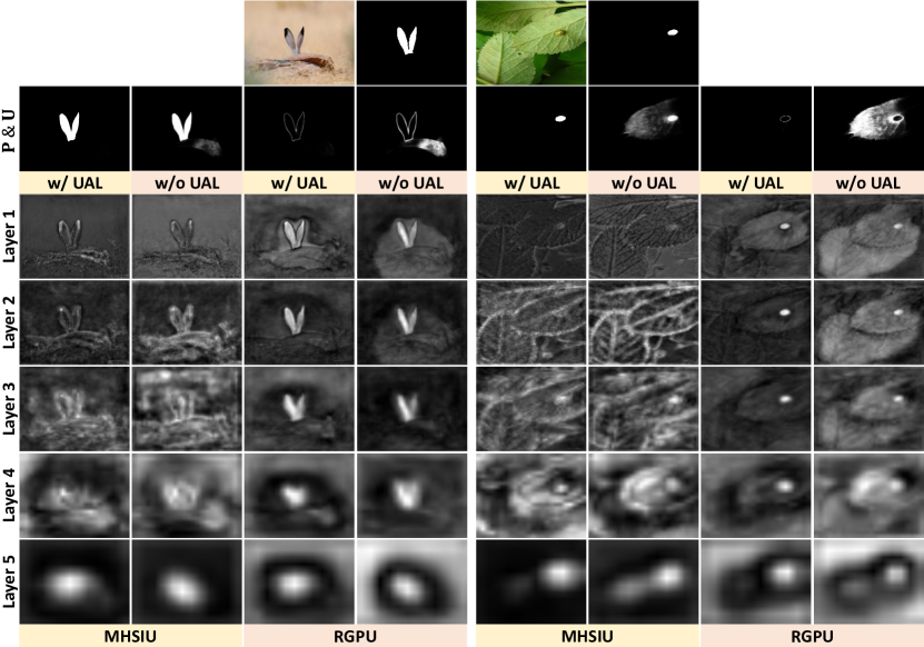
Figure 10: Intermediate feature maps from different stages of the scale merging subnetwork and the hierarchical difference propagation decoder for showing the effects of the proposed components. $\mathbf{P}$: Prediction of the model; $\mathbf{U}$: Uncertainty map generated by $\Phi_{pow}^{2}(x)$ as stated in Sec. 4.3.5.

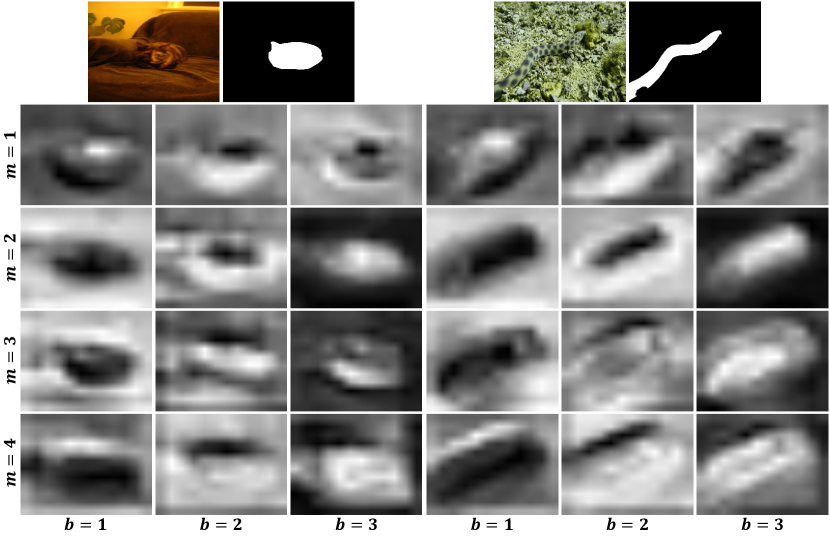
Figure 11: Spatial attention patterns from different heads $\{m=i\}^{M}_{i=1}$ corresponding to all branches $\{b=i\}^{3}_{i=1}$ in the deepest MHSIU.

4.2 Comparisons with State-of-the-arts

In order to evaluate the proposed method, we construct a comparison of it with several recent state-of-the-art image-based and video-based methods, including [27, 28, 29, 37, 34, 38, 35, 15, 1, 30, 31, 39, 14, 32, 33, 40, 41, 42, 43, 73, 74, 75, 13]. The results of all these methods come from existing public data or are generated by models retrained with the corresponding code. The comparison of the proposed method is summarized in Tab. I, Tab. II, and Fig. 6, and the qualitative performance of all methods is shown in Fig. 7 and Fig. 8.

Quantitative Evaluation Tab. I and Tab. II show the detailed comparison results for image and video COD tasks, respectively. It can be seen that the proposed model consistently and significantly surpasses recent methods on all datasets without relying on any post-processing tricks. Compared with the recent several best methods with different backbones, ZoomNet [15], DGNet [33] and SARNet [43] for image COD and STL-Net-LT [13] for video COD, although they have suppressed other existing methods, our method still shows the obvious improvement over the conference version [15] and the performance advantages over recent methods on these datasets. Besides, PR, F_β and E_m curves marked by the red color in Fig. 6 also demonstrate the effectiveness of the proposed method. The flatness of the F_β and E_m curves reflects the consistency and uniformity of the prediction. Our curves are almost horizontal, which can be attributed to the effect of the proposed UAL. It drives the predictions to be more polarized and reduces the ambiguity.

Qualitative Evaluation Visual comparisons of different methods on several typical samples are shown in Fig. 7 and Fig. 8. They present the complexity in different aspects, such as small objects (Row 3-5), middle objects (Row 1 and 2), big objects (Row 6-8), occlusions (Row 1 and 6), background interference (Row 1-3 and 6-8), and indefinable boundaries (Row 2, 3, and 5) in Fig. 7, and motion blur in Fig. 8. These results intuitively show the superior performance of the proposed method. In addition, it can be noticed that our predictions have clearer and more complete object regions, sharper contours, and better temporal consistency.

4.3 Ablation Studies

In this section, we perform comprehensive ablation analyses on different components. Because COD10K is the most widely-used large-scale COD dataset, and contains various objects and scenes, all subsequent ablation experiments are carried out on it.

TABLE IV: Comparisons of mixed and single scale input schemes on COD10K and NC4K. All models are based on the baseline model in Tab. III.

		COD10K					NC4K
Input Scale	Strategy	Sm $\uparrow$	F${}^{\omega}_{\beta}$ $\uparrow$	MAE $\downarrow$	Fβ $\uparrow$	Em $\uparrow$	Sm $\uparrow$	F${}^{\omega}_{\beta}$ $\uparrow$	MAE $\downarrow$	Fβ $\uparrow$	Em $\uparrow$	ARG
$1.0\times$	—	0.826	0.677	0.035	0.724	0.903	0.850	0.756	0.049	0.800	0.912	0.00%
$0.5\times$	—	0.761	0.552	0.049	0.611	0.860	0.810	0.686	0.061	0.737	0.882	$\downarrow$11.36%
$0.5\times,1.0\times$	Addition	0.827	0.672	0.034	0.722	0.910	0.858	0.765	0.046	0.805	0.918	$\uparrow$1.02%
$0.5\times,1.0\times$	MHSIU	0.833	0.689	0.033	0.735	0.911	0.857	0.768	0.046	0.808	0.916	$\uparrow$1.73%
$1.5\times$	—	0.850	0.717	0.031	0.764	0.921	0.856	0.769	0.048	0.810	0.913	$\uparrow$2.80%
$0.5\times,1.5\times$	Addition	0.843	0.715	0.032	0.760	0.920	0.858	0.770	0.047	0.812	0.918	$\uparrow$2.68%
$0.5\times,1.5\times$	MHSIU	0.853	0.719	0.031	0.763	0.922	0.862	0.774	0.046	0.814	0.918	$\uparrow$3.39%
$1.0\times,1.5\times$	Addition	0.852	0.717	0.031	0.761	0.924	0.864	0.776	0.046	0.814	0.919	$\uparrow$3.40%
$1.0\times,1.5\times$	MHSIU	0.856	0.722	0.030	0.767	0.927	0.866	0.780	0.045	0.819	0.920	$\uparrow$4.14%
$0.5\times,1.0\times,1.5\times$	Addition	0.849	0.719	0.030	0.763	0.923	0.863	0.782	0.043	0.819	0.921	$\uparrow$4.29%
$0.5\times,1.0\times,1.5\times$	MHSIU	0.861	0.734	0.029	0.773	0.924	0.875	0.792	0.042	0.826	0.925	$\uparrow$5.46%

TABLE V: Comparisons of different increasing strategies of $\lambda$. $\lambda_{const}$: A constant value and it is set to $1$. $t$ and $T$: The current and total number of iterations, respectively. $\lambda_{min}$ and $\lambda_{max}$: The minimum and maximum values of $\lambda$, and they are set to $0$ and $1$ in our experiments. “$\star_{t_{min}\rightarrow t_{max}}$”: The increasing interval in the iterations is $[t_{min},t_{max}]$, where $\lambda=\lambda_{min}$ when $t\leq t_{min}$, and $\lambda=\lambda_{max}$ when $t\geq t_{max}$.

		COD10K					NC4K
Strategy	$\lambda$	Sm $\uparrow$	F${}^{\omega}_{\beta}$ $\uparrow$	MAE $\downarrow$	Fβ $\uparrow$	Em $\uparrow$	Sm $\uparrow$	F${}^{\omega}_{\beta}$ $\uparrow$	MAE $\downarrow$	Fβ $\uparrow$	Em $\uparrow$
Cosine0→T		0.861	0.768	0.026	0.801	0.925	0.874	0.816	0.037	0.846	0.928
Cosine0.3T→0.7T	$\lambda_{min}+\frac{1}{2}(1-\cos(\frac{t-t_{min}}{t_{max}-t_{min}}\pi))(\lambda_{max}-\lambda_{min})$	0.858	0.767	0.025	0.798	0.925	0.870	0.813	0.037	0.841	0.924
Linear0→T		0.859	0.767	0.026	0.801	0.926	0.870	0.814	0.037	0.843	0.927
Linear0.3T→0.7T	$\lambda_{min}+\frac{t-t_{min}}{t_{max}-t_{min}}(\lambda_{max}-\lambda_{min})$	0.856	0.766	0.026	0.799	0.924	0.869	0.813	0.038	0.843	0.924
Constant	$\lambda_{const}$	0.859	0.767	0.025	0.800	0.928	0.868	0.811	0.039	0.839	0.924

TABLE VI: Different forms of the proposed UAL. Form 0 is our model without UAL. “—”: Unable to converge. Form 1.5 is used by default because of its balanced performance. Their curves are shown in Fig. 5.

			COD10K-TE					NC4K
No.	Form	$\mathbf{\alpha}$	$S_{m}~{}\uparrow$	$F^{\omega}_{\beta}~{}\uparrow$	MAE $\downarrow$	$F_{\beta}~{}\uparrow$	$E_{m}~{}\uparrow$	$S_{m}~{}\uparrow$	$F^{\omega}_{\beta}~{}\uparrow$	MAE $\downarrow$	$F_{\beta}~{}\uparrow$	$E_{m}~{}\uparrow$
0	✗	✗	0.861	0.734	0.029	0.773	0.924	0.875	0.792	0.042	0.826	0.925
1.1, 1.2, 1.3		1/8, 1/4, 1/2	—	—	—	—	—	—	—	—	—	—
1.4		1	0.859	0.762	0.026	0.795	0.923	0.870	0.810	0.039	0.841	0.926
1.5		2	0.861	0.768	0.026	0.801	0.925	0.874	0.816	0.037	0.846	0.928
1.6		4	0.857	0.768	0.027	0.802	0.923	0.868	0.815	0.038	0.844	0.925
1.7	$\Phi_{pow}^{\alpha}(x)=1-|2x-1|^{\alpha}$	8	0.859	0.767	0.026	0.802	0.924	0.867	0.814	0.038	0.843	0.923
2.1		1/8	0.866	0.741	0.027	0.782	0.933	0.875	0.794	0.041	0.828	0.926
2.2		1/4	0.862	0.736	0.028	0.777	0.928	0.876	0.794	0.041	0.828	0.926
2.3		1/2	0.863	0.742	0.028	0.781	0.930	0.876	0.798	0.040	0.831	0.927
2.4		1	0.863	0.753	0.026	0.790	0.927	0.873	0.802	0.039	0.834	0.925
2.5		2	0.862	0.762	0.026	0.797	0.927	0.873	0.810	0.038	0.841	0.928
2.6		4	0.861	0.752	0.027	0.790	0.925	0.872	0.803	0.040	0.835	0.925
2.7	$\Phi_{exp}^{\alpha}(x)=e^{-(\alpha(x-0.5))^{2}}$	8	0.861	0.737	0.028	0.778	0.929	0.874	0.793	0.041	0.827	0.926
3	BCE w/ $\omega=1+\Phi_{pow}^{2}(x)$	2	0.861	0.737	0.028	0.777	0.928	0.873	0.791	0.041	0.825	0.926

4.3.1 Effectiveness of Proposed Modules

In the proposed model, both the MHSIU and the RGPU are very important structures. We install them one by one on the baseline model to evaluate their performance. The results are shown in Tab. III. Note that only the inputs of the main scale are used in our baseline “0” and the models “1.x”. As can be seen, our baseline shows a good performance, probably due to the more reasonable network architecture. From the table, it can be seen that the two proposed modules make a significant contribution to the performance when compared to the baseline. Besides, the visual results in Fig. 9 show that the two modules can benefit each other and reduce their errors to locate and distinguish objects more accurately. These components effectively help the model to excavate and distill the critical and valuable semantics and improve the capability of distinguishing hard objects. Under the cooperation between the proposed modules and the proposed loss function, ZoomNeXt can completely capture the camouflaged objects of different scales and generate the predictions with higher consistency.

4.3.2 Number of Groups in RGPU and Heads in MHSIU

RGPU The recursive iteration strategy in the proposed RGPU stimulates the potential semantic diversity of feature representation. The results in Tab. III show the impact of different number of iteration groups on performance. Although increasing the number of groups introduces more parameters and computation, the performance does not keep increasing. It can be seen from the results that the best performance appears when the number of groups is equal to 6 and also achieves a good balance between performance and efficiency. So we use 6 groups as the default setting in all RGPUs.

MHSIU As shown in Fig. 11, the multi-head paradigm of the MHSIU further enriches the spatial pattern of attention to fine-grained information in different scale spaces. We list the efficiency and performance of different settings in Tab. III. The comparison shows that an increase in the number of heads improves computing efficiency and even performance. The best performance appears when the number of heads is set to 4, which is also the choice in other experiments.

The above experiments reflect from the side that the increase of model complexity does not necessarily lead to the improvement of performance, which also depends on more reasonable structural designs.

4.3.3 Temporal Conditional Computation

Our model introduces the temporal conditional computation, i.e., difference-aware adaptive routing mechanism, which unifies the feature processing pipelines of image and video tasks into the same framework. In Tab. II, we show the performance corresponding to different versions of the model on the video COD task. Since there is no difference in the time dimension when only a single frame is input, the corresponding model only uses static processing nodes. As more frames are fed, adaptively activated network nodes by differential information for the inter-frame interaction further improve the performance on video COD.

4.3.4 Mixed-scale Input Scheme

Our model is designed to mimic the behavior of “zooming in and out”. The feature expression is enriched by combining the scale-specific information from different scales. In Fig. 10, the intermediate features from the deep MHSIU modules show that our mixed-scale scheme plays a positive and important role in locating the camouflaged object. To analyze the role of different scales, we summarize the performance of different combination forms on two large-scale datasets COD10K [27] and NC4K [28] in Tab. IV. The proposed scheme performs better than the single-scale one and simply mixed one. This verifies the rationality of such a design for the COD task.

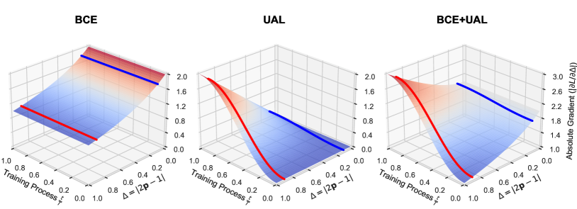
(a) Gradient landscapes.

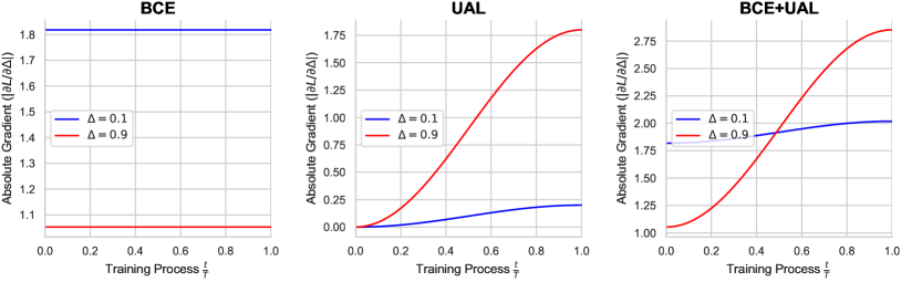
(b) Gradient curves.

Figure 12: Gradient landscapes and curves of the binary cross entropy (BCE) loss and our uncertainty awareness loss (UAL) scheduled by cosine with respect to the measure $\Delta=|2\mathbf{p}-1|$ as in Equ. 3 and the training progress $\frac{t}{T}$, where $t$ and $T$ denote the current and overall iteration steps.

4.3.5 Forms of Loss Function

Options of Setting $\lambda$ We compare three strategies and the results are listed in Tab. V, in which the increasing cosine strategy achieves the best performance. This may be due to the advantage of its smooth change process. This smooth intensity warm-up strategy of UAL motivates the model to take advantage of UAL in improving the learning process and to mitigate the possible negative interference of UAL on BCE due to the lower accuracy of the model during the early stage of training.

Forms of UAL Different forms of UAL are listed in Tab. VI and the corresponding curves are illustrated in Fig. 5. As can be seen, Form 1.5 has a more balanced performance. Also, it is worth noting that, when $\Delta$ approaches 1, the form, which can maintain a larger gradient, will obtain better performance in terms of F${}^{\omega}_{\beta}$, MAE, and F_β.

Gradient of Loss Further, from the gradient of the loss function illustrated in Fig. 12, there is a good collaboration between the proposed UAL and BCE. In the early training phase, the UAL is suppressed and the gradient is dominated by the BCE, thus facilitating a more stable optimization. However, in the later stage, the gradient of UAL is inversely proportional to $\Delta$ representing the certainty of the prediction. Such a design enables UAL to speed up updating simple samples. At the same time, it does not rashly adjust difficult samples, because they need more guidance from the ground truth.

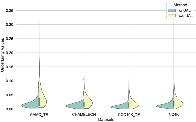
Figure 13: Visual comparison based on the violin plot for the proposed model with/without UAL. It counts the uncertainty measure of the prediction results for four image COD datasets, CAMO-TE [26], CHAMELEON [76], COD10K [27], and NC4K [28]. Better performance requires that the overall uncertainty distribution tends more toward zero. It is best to zoom in for more details.

4.3.6 Effectiveness of UAL

Fig. 9 and Fig. 10 intuitively show that the UAL greatly reduces the ambiguity caused by the interference from the background. We also visualize the uncertainty measure, i.e., UAL, of all results on four image COD datasets in Fig. 13. In Fig. 13, the peaks of the model “w/o UAL” are flatter and more upward, which means that there are more visually blurred/uncertain predictions. Besides, in the corresponding feature visualization in Fig. 10, there is clear background interference in “w/o UAL” due to the complex scenarios and blurred edges, which are extremely prone to yield false positive predictions. However, when UAL is introduced, it can be seen in Fig. 13 that the peaks of “w/ UAL” are sharper than the one of “w/o UAL”, that is, most pixel values approach two extremes and they have higher confidence. And the feature maps in Fig. 10 become more discriminative and present a more compact and complete response in the regions of camouflaged objects.

5 Conclusion

In this paper, we propose ZoomNeXt by imitating the behavior of human beings to zoom in and out on images and videos. This process actually considers the differentiated expressions about the scene from different scales, which helps to improve the understanding and judgment of camouflaged objects. We first filter and aggregate scale-specific features through the scale merging subnetwork to enhance feature representation. Next, in the hierarchical difference propagation decoder, the strategies of grouping, mixing, and fusion further mine the mixed-scale semantics. Lastly, we introduce the uncertainty awareness loss to penalize the ambiguity of the prediction. And, to the best of our knowledge, we are the first to unify the pipelines of image and video COD into a single framework. Extensive experiments verify the effectiveness of the proposed method in both the image and video COD tasks with superior performance to existing state-of-the-art methods.

References

- [1] D.-P. Fan, G.-P. Ji, M.-M. Cheng, and L. Shao, “Concealed object detection,” IEEE Transactions on Pattern Analysis and Machine Intelligence, 2021.
- [2] R. Pérez-de la Fuente, X. Delclòs, E. Peñalver, M. Speranza, J. Wierzchos, C. Ascaso, and M. S. Engel, “Early evolution and ecology of camouflage in insects,” PNAS, 2012.
- [3] G.-P. Ji, G. Xiao, Y.-C. Chou, D.-P. Fan, K. Zhao, G. Chen, and L. Van Gool, “Video polyp segmentation: A deep learning perspective,” Machine Intelligence Research, 2022.
- [4] D.-P. Fan, G.-P. Ji, T. Zhou, G. Chen, H. Fu, J. Shen, and L. Shao, “Pranet: Parallel reverse attention network for polyp segmentation,” in International Conference on Medical Image Computing and Computer-Assisted Intervention, 2020.
- [5] X. Zhao, L. Zhang, and H. Lu, “Automatic polyp segmentation via multi-scale subtraction network,” in International Conference on Medical Image Computing and Computer-Assisted Intervention. Springer, 2021.
- [6] D.-P. Fan, T. Zhou, G.-P. Ji, Y. Zhou, G. Chen, H. Fu, J. Shen, and L. Shao, “Inf-net: Automatic covid-19 lung infection segmentation from ct images,” IEEE Transactions on Medical Imaging, 2020.
- [7] L. Li, J. Liu, S. Wang, X. Wang, and T.-Z. Xiang, “Trichomonas vaginalis segmentation in microscope images,” in International Conference on Medical Image Computing and Computer-Assisted Intervention. Springer, 2022, pp. 68–78.
- [8] L. Liu, R. Wang, C. Xie, P. Yang, F. Wang, S. Sudirman, and W. Liu, “Pestnet: An end-to-end deep learning approach for large-scale multi-class pest detection and classification,” IEEE Access, 2019.
- [9] M. Rizzo, M. Marcuzzo, A. Zangari, A. Gasparetto, and A. Albarelli, “Fruit ripeness classification: A survey,” Artificial Intelligence in Agriculture, 2023.
- [10] D.-P. Fan, G.-P. Ji, P. Xu, M.-M. Cheng, C. Sakaridis, and L. Van Gool, “Advances in deep concealed scene understanding,” Visual Intelligence, 2023.
- [11] H. Lamdouar, C. Yang, W. Xie, and A. Zisserman, “Betrayed by motion: Camouflaged object discovery via motion segmentation,” in Proceedings of Asian Conference on Computer Vision, 2021.
- [12] P. Bideau and E. Learned-Miller, “It’s moving! a probabilistic model for causal motion segmentation in moving camera videos,” in Proceedings of European Conference on Computer Vision, 2016.
- [13] X. Cheng, H. Xiong, D.-P. Fan, Y. Zhong, M. Harandi, T. Drummond, and Z. Ge, “Implicit motion handling for video camouflaged object detection,” in Proceedings of IEEE Conference on Computer Vision and Pattern Recognition, 2022.
- [14] B. Yin, X. Zhang, Q. Hou, B.-Y. Sun, D.-P. Fan, and L. Van Gool, “Camoformer: Masked separable attention for camouflaged object detection,” arXiv preprint arXiv:2212.06570, 2022.
- [15] Y. Pang, X. Zhao, T.-Z. Xiang, L. Zhang, and H. Lu, “Zoom in and out: A mixed-scale triplet network for camouflaged object detection,” in Proceedings of IEEE Conference on Computer Vision and Pattern Recognition, 2022.
- [16] T. Lindeberg, Scale-space theory in computer vision. Springer Science & Business Media, 1994.
- [17] ——, “Feature detection with automatic scale selection,” International Journal of Computer Vision, vol. 30, pp. 79–116, 1998.
- [18] A. Witkin, “Scale-space filtering: A new approach to multi-scale description,” in International Conference on Acoustics, Speech and Signal Processing, Mar. 1984.
- [19] M. Stevens and S. Merilaita, “Animal camouflage: Current issues and new perspectives,” Philosophical transactions of the Royal Society of London. Series B, Biological sciences, Dec. 2008.
- [20] Z. Huang, T.-Z. Xiang, H.-X. Chen, and H. Dai, “Scribble-based boundary-aware network for weakly supervised salient object detection in remote sensing images,” ISPRS Journal of Photogrammetry and Remote Sensing, vol. 191, pp. 290–301, 2022.
- [21] H. Bi, R. Wu, Z. Liu, H. Zhu, C. Zhang, and T.-Z. Xiang, “Cross-modal hierarchical interaction network for rgb-d salient object detection,” Pattern Recognition, vol. 136, p. 109194, 2023.
- [22] A. Borji, M.-M. Cheng, Q. Hou, H. Jiang, and J. Li, “Salient object detection: A survey,” Computational Visual Media, 2014.
- [23] W. Wang, Q. Lai, H. Fu, J. Shen, H. Ling, and R. Yang, “Salient object detection in the deep learning era: An in-depth survey,” IEEE Transactions on Pattern Analysis and Machine Intelligence, 2021.
- [24] T. Zhou, D.-P. Fan, M.-M. Cheng, J. Shen, and L. Shao, “Rgb-d salient object detection: A survey,” Computational Visual Media, 2021.
- [25] T. Wang, Y. Piao, X. Li, L. Zhang, and H. Lu, “Deep learning for light field saliency detection,” in Proceedings of the IEEE International Conference on Computer Vision, 2019.
- [26] T.-N. Le, T. V. Nguyen, Z. Nie, M.-T. Tran, and A. Sugimoto, “Anabranch network for camouflaged object segmentation,” Computer Vision and Image Understanding, 2019.
- [27] D.-P. Fan, G.-P. Ji, G. Sun, M.-M. Cheng, J. Shen, and L. Shao, “Camouflaged object detection,” in Proceedings of IEEE Conference on Computer Vision and Pattern Recognition, 2020.
- [28] Y. Lyu, J. Zhang, Y. Dai, A. Li, B. Liu, N. Barnes, and D.-P. Fan, “Simultaneously localize, segment and rank the camouflaged objects,” in Proceedings of IEEE Conference on Computer Vision and Pattern Recognition, 2021.
- [29] Q. Zhai, X. Li, F. Yang, C. Chen, H. Cheng, and D.-P. Fan, “Mutual graph learning for camouflaged object detection,” in Proceedings of IEEE Conference on Computer Vision and Pattern Recognition, 2021.
- [30] H. Zhu, P. Li, H. Xie, X. Yan, D. Liang, D. Chen, M. Wei, and J. Qin, “I can find you! boundary-guided separated attention network for camouflaged object detection,” in AAAI Conference on Artificial Intelligence, 2022.
- [31] Y. Sun, S. Wang, C. Chen, and T.-Z. Xiang, “Boundary-guided camouflaged object detection,” in International Joint Conference on Artificial Intelligence, 2022.
- [32] C. He, K. Li, Y. Zhang, L. Tang, Y. Zhang, Z. Guo, and X. Li, “Camouflaged object detection with feature decomposition and edge reconstruction,” in Proceedings of IEEE Conference on Computer Vision and Pattern Recognition, 2023.
- [33] G.-P. Ji, D.-P. Fan, Y.-C. Chou, D. Dai, A. Liniger, and L. Van Gool, “Deep gradient learning for efficient camouflaged object detection,” Machine Intelligence Research, 2023.
- [34] A. Li, J. Zhang, Y. Lyu, B. Liu, T. Zhang, and Y. Dai, “Uncertainty-aware joint salient object and camouflaged object detection,” in Proceedings of IEEE Conference on Computer Vision and Pattern Recognition, 2021.
- [35] F. Yang, Q. Zhai, X. Li, R. Huang, A. Luo, H. Cheng, and D.-P. Fan, “Uncertainty-guided transformer reasoning for camouflaged object detection,” in Proceedings of the IEEE International Conference on Computer Vision, 2021.
- [36] Y. Zhang, J. Zhang, W. Hamidouche, and O. Deforges, “Predictive uncertainty estimation for camouflaged object detection,” IEEE Transactions on Image Processing, 2023.
- [37] H. Mei, G.-P. Ji, Z. Wei, X. Yang, X. Wei, and D.-P. Fan, “Camouflaged object segmentation with distraction mining,” in Proceedings of IEEE Conference on Computer Vision and Pattern Recognition, Jun. 2021.
- [38] Y. Sun, G. Chen, T. Zhou, Y. Zhang, and N. Liu, “Context-aware cross-level fusion network for camouflaged object detection,” in International Joint Conference on Artificial Intelligence, 2021.
- [39] Q. Jia, S. Yao, Y. Liu, X. Fan, R. Liu, and Z. Luo, “Segment, magnify and reiterate: Detecting camouflaged objects the hard way,” in Proceedings of IEEE Conference on Computer Vision and Pattern Recognition, 2022.
- [40] Z. Huang, H. Dai, T.-Z. Xiang, S. Wang, H.-X. Chen, J. Qin, and H. Xiong, “Feature shrinkage pyramid for camouflaged object detection with transformers,” in Proceedings of IEEE Conference on Computer Vision and Pattern Recognition, 2023.
- [41] X. Hu, S. Wang, X. Qin, H. Dai, W. Ren, D. Luo, Y. Tai, and L. Shao, “High-resolution iterative feedback network for camouflaged object detection,” in AAAI Conference on Artificial Intelligence, 2023.
- [42] Y. Liu, H. Li, J. Cheng, and X. Chen, “Mscaf-net: A general framework for camouflaged object detection via learning multi-scale context-aware features,” IEEE Transactions on Circuits and Systems for Video Technology, 2023.
- [43] H. Xing, Y. Wang, X. Wei, H. Tang, S. Gao, and W. Zhang, “Go closer to see better: Camouflaged object detection via object area amplification and figure-ground conversion,” IEEE Transactions on Circuits and Systems for Video Technology, 2023.
- [44] J. Yan, T.-N. Le, K.-D. Nguyen, M.-T. Tran, T.-T. Do, and T. V. Nguyen, “Mirrornet: Bio-inspired camouflaged object segmentation,” IEEE Access, 2021.
- [45] Y. Bengio, “Deep learning of representations: Looking forward,” in International Conference on Statistical Language and Speech Processing, 2013.
- [46] R. A. Jacobs, M. I. Jordan, S. J. Nowlan, and G. E. Hinton, “Adaptive mixtures of local experts,” Neural Computation, Feb. 1991.
- [47] N. M. Shazeer, A. Mirhoseini, K. Maziarz, A. Davis, Q. V. Le, G. E. Hinton, and J. Dean, “Outrageously large neural networks: The sparsely-gated mixture-of-experts layer,” ArXiv, 2017.
- [48] H. Hazimeh, Z. Zhao, A. Chowdhery, M. Sathiamoorthy, Y. Chen, R. Mazumder, L. Hong, and E. Chi, “Dselect-k: Differentiable selection in the mixture of experts with applications to multi-task learning,” in International Conference on Neural Information Processing Systems, 2021.
- [49] Y. Lou, F. Xue, Z. Zheng, and Y. You, “Cross-token modeling with conditional computation,” arXiv preprint arXiv:2109.02008, 2021.
- [50] C. Riquelme, J. Puigcerver, B. Mustafa, M. Neumann, R. Jenatton, A. S. Pinto, D. Keysers, and N. Houlsby, “Scaling vision with sparse mixture of experts,” arXiv preprint arXiv:2106.05974, 2021.
- [51] S. Shen, Z. Yao, C. Li, T. Darrell, K. Keutzer, and Y. He, “Scaling vision-language models with sparse mixture of experts,” arXiv preprint arXiv:2303.07226, 2023.
- [52] E. Adelson, C. Anderson, J. Bergen, P. Burt, and J. Ogden, “Pyramid methods in image processing,” RCA Eng., Nov. 1983.
- [53] T.-Y. Lin, P. Dollár, R. Girshick, K. He, B. Hariharan, and S. Belongie, “Feature pyramid networks for object detection,” in Proceedings of IEEE Conference on Computer Vision and Pattern Recognition, 2017.
- [54] K. He, X. Zhang, S. Ren, and J. Sun, “Spatial pyramid pooling in deep convolutional networks for visual recognition,” IEEE Transactions on Pattern Analysis and Machine Intelligence, 2015.
- [55] S. Ren, K. He, R. Girshick, and J. Sun, “Faster r-cnn: towards real-time object detection with region proposal networks,” IEEE Transactions on Pattern Analysis and Machine Intelligence, 2016.
- [56] X. Zhao, Y. Pang, J. Yang, L. Zhang, and H. Lu, “Multi-source fusion and automatic predictor selection for zero-shot video object segmentation,” in Proceedings of the ACM International Conference on Multimedia, 2021.
- [57] J. Long, E. Shelhamer, and T. Darrell, “Fully convolutional networks for semantic segmentation,” in Proceedings of IEEE Conference on Computer Vision and Pattern Recognition, 2015.
- [58] O. Ronneberger, P. Fischer, and T. Brox, “U-net: Convolutional networks for biomedical image segmentation,” in International Conference on Medical Image Computing and Computer-Assisted Intervention, 2015.
- [59] J.-J. Liu, Q. Hou, M.-M. Cheng, J. Feng, and J. Jiang, “A simple pooling-based design for real-time salient object detection,” in Proceedings of IEEE Conference on Computer Vision and Pattern Recognition, 2019.
- [60] Y. Pang, X. Zhao, L. Zhang, and H. Lu, “Multi-scale interactive network for salient object detection,” in Proceedings of IEEE Conference on Computer Vision and Pattern Recognition, Jun. 2020.
- [61] X. Zhao, Y. Pang, L. Zhang, H. Lu, and L. Zhang, “Suppress and balance: A simple gated network for salient object detection,” in Proceedings of European Conference on Computer Vision, 2020.
- [62] W. Ji, G. Yan, J. Li, Y. Piao, S. Yao, M. Zhang, L. Cheng, and H. Lu, “Dmra: Depth-induced multi-scale recurrent attention network for rgb-d saliency detection,” IEEE Transactions on Image Processing, 2022.
- [63] Y. Pang, L. Zhang, X. Zhao, and H. Lu, “Hierarchical dynamic filtering network for rgb-d salient object detection,” in Proceedings of European Conference on Computer Vision, 2020.
- [64] X. Zhao, L. Zhang, Y. Pang, H. Lu, and L. Zhang, “A single stream network for robust and real-time rgb-d salient object detection,” in Proceedings of European Conference on Computer Vision, 2020.
- [65] X. Zhao, Y. Pang, L. Zhang, H. Lu, and X. Ruan, “Self-supervised pretraining for rgb-d salient object detection,” in AAAI Conference on Artificial Intelligence, 2022.
- [66] K. He, X. Zhang, S. Ren, and J. Sun, “Deep residual learning for image recognition,” in Proceedings of IEEE Conference on Computer Vision and Pattern Recognition, 2016.
- [67] M. Tan and Q. Le, “Efficientnet: Rethinking model scaling for convolutional neural networks,” in Proceedings of the International Conference on Machine Learning, 2019.
- [68] W. Wang, E. Xie, X. Li, D.-P. Fan, K. Song, D. Liang, T. Lu, P. Luo, and L. Shao, “Pvt v2: Improved baselines with pyramid vision transformer,” Computational Visual Media, vol. 8, no. 3, pp. 415–424, 2022.
- [69] A. Vaswani, N. Shazeer, N. Parmar, J. Uszkoreit, L. Jones, A. N. Gomez, u. Kaiser, and I. Polosukhin, “Attention is all you need,” in International Conference on Neural Information Processing Systems, 2017.
- [70] J.-X. Zhao, J.-J. Liu, D.-P. Fan, Y. Cao, J. Yang, and M.-M. Cheng, “Egnet: Edge guidance network for salient object detection,” in Proceedings of the IEEE International Conference on Computer Vision, 2019.
- [71] X. Qin, Z. Zhang, C. Huang, C. Gao, M. Dehghan, and M. Jagersand, “Basnet: Boundary-aware salient object detection,” in Proceedings of IEEE Conference on Computer Vision and Pattern Recognition, 2019.
- [72] Z. Wu, L. Su, and Q. Huang, “Cascaded partial decoder for fast and accurate salient object detection,” in Proceedings of IEEE Conference on Computer Vision and Pattern Recognition, 2019.
- [73] G.-P. Ji, Y.-C. Chou, D.-P. Fan, G. Chen, D. Jha, H. Fu, and L. Shao, “Progressively normalized self-attention network for video polyp segmentation,” in International Conference on Medical Image Computing and Computer-Assisted Intervention, 2021.
- [74] C. Yang, H. Lamdouar, E. Lu, A. Zisserman, and W. Xie, “Self-supervised video object segmentation by motion grouping,” in 2021 IEEE/CVF International Conference on Computer Vision (ICCV), 2021.
- [75] ——, “Self-supervised video object segmentation by motion grouping,” in Proceedings of the IEEE International Conference on Computer Vision, 2021.
- [76] P. Skurowski, H. Abdulameer, J. Błaszczyk, T. Depta, A. Kornacki, and P. Kozieł, “Animal camouflage analysis: Chameleon database,” 2017, http://kgwisc.aei.polsl.pl/index.php/pl/dataset/63-animal-camouflage-analysis.
- [77] Y. Pang, “Pysodmetrics: A simple and efficient implementation of sod metrcis,” https://github.com/lartpang/PySODMetrics, 2020.
- [78] ——, “Pysodevaltoolkit: A python-based evaluation toolbox for salient object detection and camouflaged object detection,” https://github.com/lartpang/PySODEvalToolkit, 2020.
- [79] D.-P. Fan, M.-M. Cheng, Y. Liu, T. Li, and A. Borji, “Structure-measure: A new way to evaluate foreground maps,” in Proceedings of the IEEE International Conference on Computer Vision, 2017.
- [80] R. Margolin, L. Zelnik-Manor, and A. Tal, “How to evaluate foreground maps?” in Proceedings of IEEE Conference on Computer Vision and Pattern Recognition, 2014.
- [81] R. Achanta, S. Hemami, F. Estrada, and S. Süsstrunk, “Frequency-tuned salient region detection,” in Proceedings of IEEE Conference on Computer Vision and Pattern Recognition, 2009.
- [82] D.-P. Fan, C. Gong, Y. Cao, B. Ren, M.-M. Cheng, and A. Borji, “Enhanced-alignment measure for binary foreground map evaluation,” in International Joint Conference on Artificial Intelligence, 2018.
- [83] A. Paszke, S. Gross, F. Massa, A. Lerer, J. Bradbury, G. Chanan, T. Killeen, Z. Lin, N. Gimelshein, L. Antiga, A. Desmaison, A. Köpf, E. Yang, Z. DeVito, M. Raison, A. Tejani, S. Chilamkurthy, B. Steiner, L. Fang, J. Bai, and S. Chintala, “Pytorch: An imperative style, high-performance deep learning library,” in International Conference on Neural Information Processing Systems, 2019.