An explicit and symmetric exponential wave integrator for the nonlinear Schrödinger equation with low regularity potential and nonlinearity

Abstract

We propose and analyze a novel symmetric exponential wave integrator (sEWI) for the nonlinear Schrödinger equation (NLSE) with low regularity potential and typical power-type nonlinearity of the form $f(\rho)=\rho^{\sigma}$, where $\rho:=|\psi|^{2}$ is the density with $\psi$ the wave function and $\sigma>0$ is the exponent of the nonlinearity. The sEWI is explicit and stable under a time step size restriction independent of the mesh size. We rigorously establish error estimates of the sEWI under various regularity assumptions on potential and nonlinearity. For "good" potential and nonlinearity ($H^{2}$-potential and $\sigma\geq 1$), we establish an optimal second-order error bound in $L^{2}$-norm. For low regularity potential and nonlinearity ($L^{\infty}$-potential and $\sigma>0$), we obtain a first-order $L^{2}$-norm error bound accompanied with a uniform $H^{2}$-norm bound of the numerical solution. Moreover, adopting a new technique of regularity compensation oscillation (RCO) to analyze error cancellation, for some non-resonant time steps, the optimal second-order $L^{2}$-norm error bound is proved under a weaker assumption on the nonlinearity: $\sigma\geq 1/2$. For all the cases, we also present corresponding fractional order error bounds in $H^{1}$-norm, which is the natural norm in terms of energy. Extensive numerical results are reported to confirm our error estimates and to demonstrate the superiority of the sEWI, including much weaker regularity requirements on potential and nonlinearity, and excellent long-time behavior with near-conservation of mass and energy.

Keywords: nonlinear Schrödinger equation, symmetric exponential wave integrator, low regularity potential, low regularity nonlinearity, error estimate

MSC classification (2020): 35Q55, 65M15, 65M70, 81Q05

1 Introduction

The nonlinear Schrödinger equation (NLSE) arises in various physical applications such as quantum physics and chemistry, Bose-Einstein condensation (BEC), laser beam propagation, plasma and particle physics [7, 28, 43, 37]. In this paper, we consider the following NLSE on a bounded domain $\Omega=\Pi_{i=1}^{d}(a_{i},b_{i})\subset\mathbb{R}^{d}$ ($d=1,2,3$) equipped with periodic boundary condition

$$\left\{\begin{aligned} &i\partial_{t}\psi(\mathbf{x},t)=-\Delta\psi(\mathbf{x},t)+V(\mathbf{x})\psi(\mathbf{x},t)+f(|\psi(\mathbf{x},t)|^{2})\psi(\mathbf{x},t),\quad\mathbf{x}\in\Omega,\ t>0,\\ &\psi(\mathbf{x},0)=\psi_{0}(\mathbf{x}),\quad\mathbf{x}\in\overline{\Omega},\end{aligned}\right.$$ (1.1)

where $t$ is time, $\mathbf{x}\in\mathbb{R}^{d}$ is the spatial coordinate, $\psi:=\psi(\mathbf{x},t)$ is a complex-valued wave function. Here, $V:=V(\mathbf{x})\in L^{\infty}(\Omega)$ is a given real-valued external potential, and $f$ is assumed to be the power-type nonlinearity given by

$$f(\rho)=\beta\rho^{\sigma},\quad\rho:=|\psi|^{2}\geq 0,$$ (1.2)

where $\beta\in\mathbb{R}$ is a given constant and $\sigma>0$ is the exponent of the nonlinearity.

There are many important dynamical properties of the solution $\psi$ to the NLSE (1.1) [6]. The NLSE (1.1) is time reversible or symmetric, i.e. it is unchanged under the change of variable in time as $t\rightarrow-t$ and taking conjugate in the equation. It is also time transverse or gauge invariant, i.e. the equation still holds under the transformation $V\rightarrow V+\alpha$ with $\alpha$ a given constant and $\psi\rightarrow\psi e^{-i\alpha t}$, which immediately implies that the density $\rho=|\psi|^{2}$ is unchanged. Moreover, the NLSE (1.1) conserves the mass

$$M(\psi(\cdot,t))=\int_{\Omega}|\psi(\mathbf{x},t)|^{2}\mathrm{d}\mathbf{x}\equiv M(\psi_{0}),\quad t\geq 0,$$ (1.3)

and the energy

$$E(\psi(\cdot,t))=\int_{\Omega}\left[|\nabla\psi(\mathbf{x},t)|^{2}+V(\mathbf{x})|\psi(\mathbf{x},t)|^{2}+F(|\psi(\mathbf{x},t)|^{2})\right]\mathrm{d}\mathbf{x}\equiv E(\psi_{0}),\quad t\geq 0,$$ (1.4)

where the interaction energy density $F(\rho)$ is given as

$$F(\rho)=\int_{0}^{\rho}f(s)\mathrm{d}s=\frac{\beta}{\sigma+1}\rho^{\sigma+1},\quad\rho\geq 0.$$ (1.5)

When the nonlinearity is chosen as the cubic nonlinearity (i.e. $\sigma=1$ in (1.2)) and the potential is chosen as the harmonic trapping potential (namely, $V(\mathbf{x})=|\mathbf{x}|^{2}/2$), the NLSE (1.1) reduces to the cubic NLSE with smooth potential, which is also known as the Gross-Pitaevskii equation (GPE), especially in the context of BEC. In this case, both $V$ and $f$ are smooth functions. While the NLSE with smooth potential and nonlinearity, such as the GPE, is prevalent, diverse physics applications require the incorporation of low regularity potential and/or nonlinearity, including discontinuous potential, disorder potential, and non-integer power nonlinearity (see [18, 19, 32, 45] and references therein for the applications).

For the cubic NLSE with sufficiently smooth initial data, many accurate and efficient numerical methods have been proposed and analyzed in the last two decades, including the finite difference time domain (FDTD) method [1, 8, 7, 6, 32], the exponential wave integrator (EWI) [9, 33, 24, 19], and the time-splitting method [16, 20, 38, 7, 27, 6, 39, 10, 22, 18]. Among these methods, the Strang time-splitting method is widely used due to its efficient implementation and the preservation of many dynamical properties including the time symmetry, time transverse invariance, dispersion relation, and mass conservation at the discrete level [6]. Recently, some low regularity integrators (LRI) are also designed for the cubic NLSE with low regularity initial data and with/without potential [41, 36, 40, 3, 21, 5, 4].

Most of the aforementioned numerical methods can be extended straightforwardly to solve the NLSE (1.1) with low regularity potential and/or nonlinearity, e.g. the FDTD method [32], the time-splitting method [34, 25, 18, 45, 17], the EWI [19] and the LRI [45, 5, 3] (different from some singular nonlinearities [12, 13, 14, 15, 44], where regularization may be needed). However, their performances deviate considerably when compared to the smooth setting. As demonstrated in [19], compared with FDTD methods, time-splitting methods and LRIs, in the presence of low regularity potential and/or nonlinearity, the Gautschi-type EWI outperforms all of them (at least at semi-discrete level). Nevertheless, it remains a first-order method and fails to preserve either the time symmetry or the conservation of mass and energy. It is of great interest to devise numerical schemes of high order that are capable of preserving the dynamical properties at discrete level. Based on the discussion above, we focus on designing and analyzing structure-preserving Gautschi-type EWIs.

In this work, we introduce a second-order explicit and symmetric Gautschi-type EWI (sEWI), which is particularly advantageous for the NLSE with low regularity potential and nonlinearity. Note that any symmetric methods are at least second order [31]. Additionally, we establish rigorous error estimates under different regularity assumptions on potential and nonlinearity, confirming the scheme’s benefits when applied to the NLSE with low regularity potential and nonlinearity.

In fact, extensive efforts have been made in the literature to design symmetric exponential integrators for the cubic NLSE, motivated by the structure-preserving properties and favorable long-time behavior of these symmetric schemes [24, 30, 31, 2, 29, 4]. However, most of them are fully implicit, which necessitates solving a fully nonlinear system at each time step. Usually, the nonlinear system is solved by fixed point iteration, which is time-consuming, especially in two dimensions (2D) and three dimensions (3D) [24, 2, 29]. Actually, if the nonlinear system is not solved up to sufficient accuracy (e.g. machine accuracy), the symmetric property of the scheme may be destroyed. Moreover, although there are some explicit symmetric schemes in the literature [30], they are only conditionally stable under certain CFL-type time step size restrictions. Additionally, all those schemes lack error estimates under low regularity assumptions on potential and nonlinearity. In contrast, our new sEWI offers several advantages—it is explicit, stable under a time step size restriction that is independent of the mesh size and has been rigorously proved to be well-suited for low regularity potential and nonlinearity.

To show the merit of our new sEWI for the NLSE with low regularity potential and nonlinearity, we rigorously establish error estimates under varying regularity assumptions on potential and nonlinearity. Main results are stated in Sections 3.1 and 4.1, and we also summarize them here:

1. under the assumption of $H^{2}$-potential, $\sigma\geq 1$ and $H^{4}$-solution, we derive an optimal second-order error bound in $L^{2}$-norm at both semi-discrete (Theorem 3.1) and fully discrete (Theorem 4.1) level;

2. under more general assumptions of $L^{\infty}$-potential, $\sigma>0$ and $H^{2}$-solution, we establish a first-order error bound in $L^{2}$-norm along with a uniform $H^{2}$-bound of the numerical solution at both semi-discrete (Theorem 3.2) and fully discrete (Theorem 4.2) level;

3. for the full-discretization scheme, the assumption on the nonlinearity in (i) can be relaxed to $\sigma\geq 1/2$ for certain non-resonant time steps (Theorem 4.3).

For first-order $L^{2}$-norm error bound in time, (ii) mirrors the first-order EWI in [19], which, to our best knowledge, requires the weakest regularity of both potential and nonlinearity, among FDTD method [32], Lei-Trotter time-splitting method [18, 17, 34, 25], and LRIs [3, 5]. In terms of the optimal second-order error bound, the assumption of the sEWI in (i) is significantly weaker than the requirement of the Strang time-splitting method which requires $H^{4}$-potential and $\sigma\geq 3/2$ (or $\sigma=1$) [20, 38, 7]. Although recent results in [17] show that, for the full-discretization of the Strang time-splitting method, it can obtain optimal $L^{2}$-norm error bound under the same assumption as the sEWI in (i), a CFL-type time step size restriction is necessary. Actually, if imposing the same time step size restriction, the regularity requirement on nonlinearity for the sEWI can be further relaxed as in (iii).

We briefly explain the idea of our proof for these results. As mentioned before, (ii) can be similarly obtained with new techniques developed in [19]. Then, with the uniform $H^{2}$-bound of the numerical solution established in (ii), one can easily prove (i) by standard Lady-Windermere’s fan argument. The proof of (iii) relies on another new technique called regularity compensation oscillation (RCO) proposed in [10, 11] for the analysis of long-time dynamics and extended in [17] to the analysis of low regularity potential and nonlinearity. Based on RCO, we estimate high frequency waves by regularity of the solution and estimate low frequency waves by error cancellation. As a result, for certain non-resonant time steps, we can obtain the optimal error bound in $L^{2}$-norm under a weaker assumption on nonlinearity. The exact solution $\psi$ still need to be in $H^{4}$, which is possible when $\sigma\geq 1/2$ with smooth initial data as numerically observed in [18, 17].

The rest of the paper is organized as follows. In Section 2, we present the explicit and symmetric exponential wave integrator (sEWI) and its spatial discretization by the Fourier spectral method. Sections 3-4 are devoted to the error estimates of the sEWI at semi-discrete level and fully discrete level, respectively. Numerical results are reported in Section 5 to confirm our error estimates. Finally, some conclusions are drawn in Section 6. Throughout the paper, we adopt standard notations of vector-valued Sobolev spaces as well as their corresponding norms. The bold letters are always used for vector-valued functions or operators. We denote by $C$ a generic positive constant independent of the mesh size $h$ and time step size $\tau$, and by $C(\alpha)$ a generic positive constant depending only on the parameter $\alpha$. The notation $A\lesssim B$ is used to represent that there exists a generic constant $C>0$, such that $|A|\leq CB$.

2 An explicit and symmetric exponential wave integrator

In this section, we introduce an explicit and symmetric exponential wave integrator (sEWI) and its spatial discretization to solve the NLSE with low regularity potential and nonlinearity. For simplicity of the presentation and to avoid heavy notations, we only carry out the analysis in one dimension (1D) and take $\Omega=(a,b)$. Generalizations to 2D and 3D are straightforward. We define the periodic Sobolev spaces as (see, e.g. [3], for the definition in phase space)

$$H^{m}_{\text{per}}(\Omega):=\{\phi\in H^{m}(\Omega):\phi^{(k)}(a)=\phi^{(k)}(b),\quad k=0,\cdots,m-1\},\quad m\in\mathbb{Z}^{+}.$$

2.1 A semi-discretization in time

For simplicity, define an operator $B$ as

$$B(v)(x):=V(x)v(x)+f(|v(x)|^{2})v(x),\quad v\in L^{2}(\Omega).$$ (2.1)

Choose a time step size $\tau>0$ and denote time steps as $t_{n}=n\tau$ for $n=0,1,\cdots$. In the following, we shall always abbreviate $\psi(\cdot,t)$ by $\psi(t)$ for simplicity when there is no confusion. By Duhamel’s formula, the exact solution $\psi$ satisfies

$$\psi(t_{n}+w)=e^{iw\Delta}\psi(t_{n})-i\int_{0}^{w}e^{i(w-s)\Delta}B(\psi(t_{n}+s))\mathrm{d}s,\quad w\in\mathbb{R}.$$ (2.2)

Multiplying $e^{-iw\Delta}$ on both sides of (2.2), we obtain

$$e^{-iw\Delta}\psi(t_{n}+w)=\psi(t_{n})-i\int_{0}^{w}e^{-is\Delta}B(\psi(t_{n}+s))\mathrm{d}s.$$ (2.3)

Taking $w=\tau$ in (2.3), we get

$$e^{-i\tau\Delta}\psi(t_{n+1})=\psi(t_{n})-i\int_{0}^{\tau}e^{-is\Delta}B(\psi(t_{n}+s))\mathrm{d}s.$$ (2.4)

Taking $w=-\tau$ in (2.3), we get

$$e^{i\tau\Delta}\psi(t_{n-1}) =\psi(t_{n})-i\int_{0}^{-\tau}e^{-is\Delta}B(\psi(t_{n}+s))\mathrm{d}s$$

$$=\psi(t_{n})+i\int_{-\tau}^{0}e^{-is\Delta}B(\psi(t_{n}+s))\mathrm{d}s.$$ (2.5)

Subtracting (2.1) from (2.4), we obtain

$$e^{-i\tau\Delta}\psi(t_{n+1})-e^{i\tau\Delta}\psi(t_{n-1})=-i\int_{-\tau}^{\tau}e^{-is\Delta}B(\psi(t_{n}+s))\mathrm{d}s.$$ (2.6)

Multiplying $e^{i\tau\Delta}$ on both sides of (2.6) yields

$$\psi(t_{n+1})=e^{2i\tau\Delta}\psi(t_{n-1})-i\int_{-\tau}^{\tau}e^{i(\tau-s)\Delta}B(\psi(t_{n}+s))\mathrm{d}s.$$ (2.7)

Applying the Gautschi-type rule to approximate the integral in (2.7), i.e. approximating $\psi(t_{n}+s)$ by $\psi(t_{n})$ and integrating out $e^{i(\tau-s)\Delta}$ exactly, we get

$$\int_{-\tau}^{\tau}e^{i(\tau-s)\Delta}B(\psi(t_{n}+s))\mathrm{d}s\approx\int_{-\tau}^{\tau}e^{i(\tau-s)\Delta}B(\psi(t_{n}))\mathrm{d}s=2\tau e^{i\tau\Delta}{\varphi_{\text{s}}}(\tau\Delta)B(\psi(t_{n})),$$ (2.8)

where ${\varphi_{\text{s}}}:\mathbb{R}\rightarrow\mathbb{R}$ is an analytic and even function defined as

$${\varphi_{\text{s}}}(\theta)=\operatorname{sinc}(\theta)=\frac{\sin(\theta)}{\theta},\qquad\theta\in\mathbb{R}.$$ (2.9)

Plugging (2.8) into (2.7) yields

$$\psi(t_{n+1})\approx e^{2i\tau\Delta}\psi(t_{n-1})-2i\tau e^{i\tau\Delta}{\varphi_{\text{s}}}(\tau\Delta)B(\psi(t_{n})).$$ (2.10)

For the first step, we apply a first-order Gautschi-type approximation as

$$\psi(t_{1})=e^{i\tau\Delta}\psi(t_{0})-i\tau\int_{0}^{\tau}e^{i(\tau-s)\Delta}B(\psi(t_{0}+s))\mathrm{d}s \approx e^{i\tau\Delta}\psi(t_{0})-i\int_{0}^{\tau}e^{i(\tau-s)\Delta}B(\psi(t_{0}))\mathrm{d}s$$

$$=e^{i\tau\Delta}\psi(t_{0})-i\tau\varphi_{1}(i\tau\Delta)B(\psi(t_{0})),$$ (2.11)

where $\varphi_{1}:\mathbb{C}\rightarrow\mathbb{C}$ is an entire function defined as

$$\varphi_{1}(z)=\frac{e^{z}-1}{z},\qquad z\in\mathbb{C}.$$ (2.12)

The operator $\varphi_{1}(i\tau\Delta)$ and $\varphi_{s}(\tau\Delta)$ are defined through their action in the Fourier space, and they satisfy $\varphi_{1}(i\tau\Delta)v,\varphi_{s}(i\tau\Delta)v\in H^{2}_{\text{per}}(\Omega)$ for all $v\in L^{2}(\Omega)$ (see (2.3) and (2.5) in [19]).

Let $\psi^{[n]}(\cdot)$ be the approximation of $\psi(\cdot,t_{n})$ for $n\geq 0$. Applying the approximations Equations 2.10 and 2.1, we obtain an explicit and symmetric exponential wave integrator (sEWI) as

$$\psi^{[n+1]} =e^{2i\tau\Delta}\psi^{[n-1]}-2i\tau e^{i\tau\Delta}{\varphi_{\text{s}}}(\tau\Delta)B(\psi^{[n]}),\quad n\geq 1,$$ (2.13)

$$\psi^{[1]} =e^{i\tau\Delta}\psi^{[0]}-i\tau\varphi_{1}(i\tau\Delta)B(\psi^{[0]}),$$

$$\psi^{[0]} =\psi_{0}.$$

One can check that the scheme is unchanged for $n\geq 1$ when exchanging $n-1$ and $n+1$ and replacing $\tau$ with $-\tau$, which implies that the scheme (2.13) is symmetric in time.

Remark 2.1.

For the computation of the first step $\psi^{[1]}$, instead of the first-order Gautschi-type EWI we present here, one may choose other methods such as the Strang time-splitting method to guarantee time symmetry in the first step, which would be beneficial in the smooth setting. However, according to the analysis in [18, 19, 17], time-splitting methods cannot give accurate approximation in the presence of low regularity potential and/or nonlinearity, and it will totally destroy the regularity of the numerical solution even for one step. Hence, if one wants a better approximation of the first step under the low regularity setting, we suggest computing $\psi^{[1]}$ "exactly" by using the first-order Gautschi-type EWI a few times with a small time step.

2.2 A full-discretization by using the Fourier spectral method in space

In this subsection, we further discretize the sEWI (2.13) in space by the Fourier spectral method to obtain a fully discrete scheme. Usually, the Fourier pseudospectral method is used for spatial discretization, which can be efficiently implemented with FFT. However, due to the low regularity of potential and/or nonlinearity, it is very hard to establish error estimates of the Fourier pseudospectral method, and it is impossible to obtain optimal error bounds in space as order reduction can be observed numerically [19, 26].

Choose a mesh size $h=(b-a)/N$ with $N$ being a positive even integer. Define the index set

$$\mathcal{T}_{N}=\left\{-\frac{N}{2},\cdots,\frac{N}{2}-1\right\},$$

and denote

$$X_{N}=\text{span}\left\{e^{i\mu_{l}(x-a)}:l\in\mathcal{T}_{N}\right\},\quad\mu_{l}=\frac{2\pi l}{b-a}.$$ (2.14)

Let $P_{N}:L^{2}(\Omega)\rightarrow X_{N}$ be the standard $L^{2}$-projection onto $X_{N}$ as

$$(P_{N}u)(x)=\sum_{l\in\mathcal{T}_{N}}\widehat{u}_{l}e^{i\mu_{l}(x-a)},\qquad x\in\overline{\Omega}=[a,b],$$ (2.15)

where $u\in L^{2}(\Omega)$ and $\widehat{u}_{l}$ are the Fourier coefficients of $u$ defined as

$$\widehat{u}_{l}=\frac{1}{b-a}\int_{a}^{b}u(x)e^{-i\mu_{l}(x-a)}\mathrm{d}x,\qquad l\in\mathbb{Z}.$$ (2.16)

Let $\psi^{n}(\cdot)$ be the numerical approximations of $\psi(\cdot,t_{n})$ for $n\geq 0$. Then an explicit and symmetric exponential wave integrator Fourier spectral method (sEWI-FS) reads

$$\widehat{(\psi^{n+1})}_{l} =e^{-2i\tau\mu_{l}^{2}}\widehat{(\psi^{n-1})}_{l}-2i\tau e^{-i\tau\mu_{l}^{2}}\varphi_{s}(\tau\mu_{l}^{2})\widehat{(B(\psi^{n}))}_{l},\quad l\in\mathcal{T}_{N},\quad n\geq 1,$$ (2.17)

$$\widehat{(\psi^{1})}_{l} =e^{-i\tau\mu_{l}^{2}}\widehat{(\psi^{0})}_{l}-i\tau\varphi_{1}(-i\tau\mu_{l}^{2})\widehat{(B(\psi^{0}))}_{l},\quad l\in\mathcal{T}_{N},$$

$$\widehat{(\psi^{0})}_{l} =\widehat{(\psi_{0})}_{l},\quad l\in\mathcal{T}_{N}.$$

Note that the numerical solution $\psi^{n}(n\geq 0)\in X_{N}$ obtained from (2.17) satisfies

$$\psi^{n+1} =e^{2i\tau\Delta}\psi^{n-1}-2i\tau e^{i\tau\Delta}\varphi_{s}(\tau\Delta)P_{N}B(\psi^{n}),\quad n\geq 1,$$ (2.18)

$$\psi^{1} =e^{i\tau\Delta}\psi^{0}-i\tau\varphi_{1}(i\tau\Delta)P_{N}B(\psi^{0}),$$

$$\psi^{0} =P_{N}\psi_{0}.$$

One may check again that when exchanging $n+1$ and $n-1$ and replacing $\tau$ by $-\tau$ in the first equation of (2.18), the equation remains unchanged, which implies that the fully discrete scheme is still time symmetric. Note that the Fourier spectral discretization of the Strang time-splitting method (which is considered in [17]) is no longer symmetric in time.

2.3 Stability

By adopting the standard Von Neumann analysis, we obtain the following linear stability of the sEWI-FS method (2.17).

Proposition 2.2.

Assume that $V(x)\equiv V_{0}\in\mathbb{R}$ and $f(\rho)\equiv f_{0}\in\mathbb{R}$. Then the sEWI-FS method (2.17) is stable when $\tau|V_{0}+f_{0}|\leq 1$.

Proof.

Noting that $B(\phi)=(V_{0}+f_{0})\phi$ and plugging

$$\widehat{(\psi^{n+1})}_{l}=\xi_{l}^{2}\widehat{(\psi^{n-1})}_{l},\quad\widehat{(\psi^{n})}_{l}=\xi_{l}\widehat{(\psi^{n-1})}_{l},\qquad l\in\mathcal{T}_{N},\quad n\geq 1,$$

into the first equation of (2.17), we obtain

$$\xi_{l}^{2}+2i\tau e^{-i\tau\mu_{l}^{2}}\varphi_{s}(\tau\mu_{l}^{2})(V_{0}+f_{0})\xi_{l}-e^{-2i\tau\mu_{l}^{2}}=0,\quad l\in\mathcal{T}_{N},$$

which implies

$$\xi_{l}=e^{-i\tau\mu_{l}^{2}}\left(-i\tau\varphi_{s}(\tau\mu_{l}^{2})(V_{0}+f_{0})\pm\sqrt{1-\tau^{2}(\varphi_{s}(\tau\mu_{l}^{2}))^{2}(V_{0}+f_{0})^{2}}\right).$$

When $\tau|V_{0}+f_{0}|\leq 1$, recalling $|\varphi_{s}(\theta)|\leq 1$, we have $1-\tau^{2}(\varphi_{s}(\tau\mu_{l}^{2}))^{2}(V_{0}+f_{0})^{2}\geq 0$ and thus

$$|\xi_{l}|=\sqrt{\tau^{2}(\varphi_{s}(\tau\mu_{l}^{2}))^{2}(V_{0}+f_{0})^{2}+1-\tau^{2}(\varphi_{s}(\tau\mu_{l}^{2}))^{2}(V_{0}+f_{0})^{2}}=1,\quad l\in\mathcal{T}_{N},$$ (2.19)

which implies the stability of the sEWI-FS method (2.17). ∎

Remark 2.3.

One can design another explicit symmetric EWI by following similar ideas for (2.13). To be precise, by taking $w=\tau$ and $w=-\tau$ in (2.2) instead of (2.3), and subtracting one from the other, one gets

$$\psi(t_{n+1})-\psi(t_{n-1}) =2i\sin(\tau\Delta)\psi(t_{n})$$

$$\quad-i\int_{0}^{\tau}\left[e^{i(\tau-s)\Delta}B(\psi(t_{n}+s))+e^{-i(\tau-s)\Delta}B(\psi(t_{n}-s))\right]\mathrm{d}s.$$ (2.20)

Similar to (2.8), approximating the integral in (2.3) with the Gautschi-type rule by applying $\psi(t_{n}+s)\approx\psi(t_{n})$ and $\psi(t_{n}-s)\approx\psi(t_{n})$, one obtains

$$\int_{0}^{\tau}\left[e^{i(\tau-s)\Delta}B(\psi(t_{n}+s))+e^{-i(\tau-s)\Delta}B(\psi(t_{n}-s))\right]\mathrm{d}s$$

$$\approx\int_{0}^{\tau}(e^{i(\tau-s)\Delta}+e^{-i(\tau-s)\Delta})B(\psi(t_{n}))\mathrm{d}s=2\tau{\varphi_{\text{s}}}(\tau\Delta)B(\psi(t_{n})),$$ (2.21)

which yields another symmetric EWI scheme as

$$\psi^{[n+1]}=\psi^{[n-1]}+2i\sin(\tau\Delta)\psi^{[n]}-2i\tau{\varphi_{\text{s}}}(\tau\Delta)B(\psi^{[n]}),\quad n\geq 1.$$ (2.22)

However, the resulting fully discrete scheme by using the Fourier spectral method in space will be only conditionally stable subject to a time step size restriction $\tau\lesssim h^{2}$. Hence, we will not consider this scheme in this paper.

3 Error estimates of the semi-discretization Equation 2.13

In this section, we shall prove error estimates for the semi-discrete scheme (2.13) under different regularity assumptions on the potential, nonlinearity and exact solution. Let $T_{\text{max}}$ be the maximal existing time of the solution to the NLSE (1.1) and take $0<T<T_{\text{max}}$ be some fixed time.

3.1 Main results

Let $\psi^{[n]}(n\geq 0)$ be obtained from (2.13). For sufficiently smooth potential and nonlinearity as well as the exact solution, we have the following optimal second-order $L^{2}$-norm error bound:

Theorem 3.1 (Optimal second-order error bound for "good" potential and nonlinearity).

Assume that $V\in H^{2}_{\text{\rm per}}(\Omega)$, $\sigma\geq 1$, and $\psi\in C([0,T];H_{\text{\rm per}}^{4}(\Omega))\cap C^{1}([0,T];H^{2}(\Omega))\cap C^{2}([0,T];L^{2}(\Omega))$. There exists $\tau_{0}>0$ sufficiently small such that when $0<\tau<\tau_{0}$, we have

$$\|\psi(\cdot,t_{n})-\psi^{[n]}\|_{L^{2}}\lesssim\tau^{2},\quad\|\psi(\cdot,t_{n})-\psi^{[n]}\|_{H^{1}}\lesssim\tau^{\frac{3}{2}},\quad 0\leq n\leq T/\tau.$$

For more general low regularity potential and/or nonlinearity, which inevitably results in low regularity of the exact solution, we have the following first-order $L^{2}$-norm error bound, which has recently been established for the first-order Gautschi-type EWI in [19].

Theorem 3.2 (Error bound for low regularity potential and/or nonlinearity).

Assume that $V\in L^{\infty}(\Omega)$, $\sigma>0$ and $\psi\in C([0,T];H^{2}_{\text{\rm per}}(\Omega))\cap C^{1}([0,T];L^{2}(\Omega))$. There exists $\tau_{0}>0$ sufficiently small such that when $0<\tau<\tau_{0}$, we have

$$\|\psi(\cdot,t_{n})-\psi^{[n]}\|_{L^{2}}\lesssim\tau,\quad\|\psi^{[n]}\|_{H^{2}}\lesssim 1,$$

$$\|\psi(\cdot,t_{n})-\psi^{[n]}\|_{H^{1}}\lesssim\sqrt{\tau},\qquad 0\leq n\leq T/\tau.$$

Remark 3.3.

Recall the results in [20, 38, 7], to obtain the second-order $L^{2}$-norm error bound of the Strang time-splitting method at semi-discrete level, it is required that $V\in H^{4}_{\text{per}}(\Omega)$ and $\sigma\geq 3/2$ (or $\sigma=1$), which is much stronger than the requirement in Theorem 3.1 of the sEWI. Similarly, in terms of the first-order $L^{2}$-norm error bound at semi-discrete level, as is already discussed in [19], the sEWI also needs significantly weaker regularity than the Lie-Trotter time-splitting method analyzed in [18].

Remark 3.4.

Regarding the assumption of Theorem 3.2, according to the results in [23, 35] (see also [18, 19, 17]), when $V\in L^{\infty}(\Omega)$ and $\sigma>0$, it can be expected that the unique exact solution $\psi\in C([0,T];H^{2}_{\text{per}}(\Omega))\cap C^{1}([0,T];L^{2}(\Omega))$ if $\psi_{0}\in H^{2}_{\text{per}}(\Omega)$ in the NLSE (1.1). The assumption of Theorem 3.1 is compatible with this assumption in the sense that the increment of differentiability orders of potential and nonlinearity are the same as the exact solution. In other words, when $V\in H^{2}_{\text{\rm per}}(\Omega)$ and $\sigma\geq 1$, if $\psi_{0}\in H^{4}_{\text{per}}(\Omega)$, one could expect $\psi\in C([0,T];H_{\text{\rm per}}^{4}(\Omega))\cap C^{1}([0,T];H^{2}(\Omega))\cap C^{2}([0,T];L^{2}(\Omega))$.

In the rest of this section, we shall prove Theorems 3.1 and 3.2. Note that the assumption of Theorem 3.2 is more general than Theorem 3.1. Hence, we start with the proof of Theorem 3.2, and the uniform $H^{2}$-bound of the numerical solution established in Theorem 3.2 will be used to simplify the proof of Theorem 3.1.

3.2 Proof of Theorem 3.2 for low regularity potential and/or nonlinearity

In this subsection, we will establish a first-order error bound for the sEWI under low regularity assumptions made in Theorem 3.2, i.e.

$$V\in L^{\infty}(\Omega),\quad\sigma>0,\quad\psi\in C([0,T];H^{2}_{\text{per}}(\Omega))\cap C^{1}([0,T];L^{2}(\Omega)).$$ (3.1)

Under similar assumptions, a first-order error bound has recently been shown for the first-order Gautschi-type EWI in [19]. Here, following a similar idea, we can prove the same first-order error bound for the sEWI.

To follow the proof for the one step method, we first rewrite the sEWI scheme (2.13) into the matrix form. For simplicity of presentation, we define $\Phi^{\tau}:[H^{2}_{\text{per}}(\Omega)]^{2}\rightarrow H^{2}_{\text{per}}(\Omega)$ as

$$\Phi^{\tau}(\phi_{1},\phi_{0})=e^{2i\tau\Delta}\phi_{0}-2i\tau e^{i\tau\Delta}{\varphi_{\text{s}}}(\tau\Delta)B(\phi_{1}),\quad\phi_{0},\phi_{1}\in H^{2}_{\text{per}}(\Omega).$$ (3.2)

Recalling (2.13), one immediately has

$$\psi^{[n+1]}=\Phi^{\tau}(\psi^{[n]},\psi^{[n-1]}),\qquad n\geq 1.$$

Introducing a semi-discrete numerical flow ${\mathbf{\Phi}}^{\tau}:[H_{\text{per}}^{2}(\Omega)]^{2}\rightarrow[H_{\text{per}}^{2}(\Omega)]^{2}$ as

$${\mathbf{\Phi}}^{\tau}\begin{pmatrix}\phi_{1}\\ \phi_{0}\end{pmatrix}=\mathbf{A}(\tau)\begin{pmatrix}\phi_{1}\\ \phi_{0}\end{pmatrix}+\tau{\mathbf{H}}(\phi_{1})=\begin{pmatrix}\Phi^{\tau}(\phi_{1},\phi_{0})\\ \phi_{1}\end{pmatrix},\quad\phi_{0},\phi_{1}\in H^{2}_{\text{per}}(\Omega),$$ (3.3)

where $\Phi^{\tau}$ is defined in (3.2) and

$$\mathbf{A}(t):=\begin{pmatrix}0&e^{2it\Delta}\\ I&0\end{pmatrix},\quad{\mathbf{H}}(\phi):=\begin{pmatrix}-2ie^{i\tau\Delta}{\varphi_{\text{s}}}(\tau\Delta)B(\phi)\\ 0\end{pmatrix},\quad\phi\in H^{2}_{\text{per}}(\Omega).$$ (3.4)

Define the semi-discrete solution vector $\mathbf{\Psi}^{[n]}(1\leq n\leq T/\tau)\in[H^{2}_{\text{per}}(\Omega)]^{2}$ as

$$\mathbf{\Psi}^{[n]}:=(\psi^{[n]},\psi^{[n-1]})^{T},\qquad 1\leq n\leq T/\tau.$$ (3.5)

Then the sEWI scheme (2.13) can be equivalently written into the matrix form as

$$\mathbf{\Psi}^{[n+1]} ={\mathbf{\Phi}}^{\tau}\left(\mathbf{\Psi}^{[n]}\right)=\mathbf{A}(\tau)\begin{pmatrix}\psi^{[n]}\\ \psi^{[n-1]}\end{pmatrix}+\tau{\mathbf{H}}(\psi^{[n]}),\quad n\geq 1$$ (3.6)

$$\mathbf{\Psi}^{[1]} =\begin{pmatrix}\psi^{[1]}\\ \psi^{[0]}\end{pmatrix}=\begin{pmatrix}e^{i\tau\Delta}\psi_{0}-i\tau\varphi_{1}(i\tau\Delta)B(\psi_{0})\\ \psi_{0}\end{pmatrix}.$$

For $1\leq n\leq T/\tau$, we also define the exact solution vector ${\mathbf{\Psi}(t_{n})}$ as

$${\mathbf{\Psi}(t_{n})}:=(\psi(t_{n}),\psi(t_{n-1}))^{T}.$$ (3.7)

We first present some estimates of the operator $B$ (2.1). The proof can be found in [17].

Lemma 3.5.

Under the assumptions $V\in L^{\infty}(\Omega)$ and $\sigma>0$, for any $v,w\in L^{2}(\Omega)$ satisfying $\|v\|_{L^{\infty}}\leq M$ and $\|w\|_{L^{\infty}}\leq M$, we have

$$\|B(v)-B(w)\|_{L^{2}}\leq C(\|V\|_{L^{\infty}},M)\|v-w\|_{L^{2}}.$$

Let $dB(\cdot)[\cdot]$ be the Gâteaux derivative defined as

$$dB(v)[w]:=\lim_{\varepsilon\rightarrow 0}\frac{B(v+\varepsilon w)-B(v)}{\varepsilon},$$ (3.8)

where the limit is taken for real $\varepsilon$ (see also [18]). Introduce a continuous function $G:\mathbb{C}\rightarrow\mathbb{C}$ as

$$G(z)=\left\{\begin{aligned} &f^{\prime}(|z|^{2})z^{2}=\beta\sigma|z|^{2\sigma-2}z^{2},&z\neq 0,\\ &0,&z=0,\end{aligned}\right.\qquad z\in\mathbb{C}.$$ (3.9)

Plugging the expression of $B$ (2.1) into (3.8), we obtain

$$dB(v)[w]=-i\left[Vw+(1+\sigma)f(|v|^{2})w+G(v)\overline{w}\right],$$ (3.10)

where we use $f^{\prime}(|z|^{2})|z|^{2}=\sigma f(|z|^{2})$ for all $z\in\mathbb{C}$ and define $G(v)(x):=G(v(x))$. Then we have

Lemma 3.6.

Under the assumptions $V\in L^{\infty}(\Omega)$ and $\sigma>0$, for any $v,w\in L^{2}(\Omega)$ satisfying $\|v\|_{L^{\infty}}\leq M$, we have

$$\|dB(v)[w]\|_{L^{2}}\leq C(\|V\|_{L^{\infty}},M)\|w\|_{L^{2}}.$$

By Lemma 3.5, for ${\mathbf{H}}$ in (3.4), using the boundedness of $e^{it\Delta}$ and ${\varphi_{\text{s}}}(t\Delta)$, we have

$$\|{\mathbf{H}}(v)-{\mathbf{H}}(w)\|_{L^{2}}\leq 2\|B(v)-B(w)\|_{L^{2}}\leq C(\|V\|_{L^{\infty}},M)\|v-w\|_{L^{2}}.$$ (3.11)

Then we shall prove Theorem 3.2. By taking $n=0$ in Proposition 3.7 in [19], noting that

$${\mathbf{\Psi}(t_{1})}-\mathbf{\Psi}^{[1]}=(\psi(t_{1}),\psi(t_{0}))^{T}-(\psi^{[1]},\psi_{0})^{T}=(\psi(t_{1})-\psi^{[1]},0)^{T},$$

we have the following error estimate of the first step.

Proposition 3.7.

Under the assumptions (3.1), we have

$$\left\|{\mathbf{\Psi}(t_{1})}-\mathbf{\Psi}^{[1]}\right\|_{H^{\alpha}}\lesssim\tau^{2-\alpha/2},\quad 0\leq\alpha\leq 2.$$

By Lemma 3.6 in [19], for $v\in C([0,\tau];L^{2}(\Omega))\cap W^{1,\infty}([0,\tau];L^{2}(\Omega))$ and

$$u_{1}=-i\int_{0}^{\tau}e^{i(\tau-s)\Delta}v(s)\mathrm{d}s,$$

we have

$$\|\Delta u_{1}\|_{L^{2}}\leq 2\|v\|_{L^{\infty}([0,\tau];L^{2})}+\tau\|\partial_{t}v\|_{L^{\infty}([0,\tau];L^{2})}.$$ (3.12)

As an immediate corollary, if $v\in C([-\tau,\tau];L^{2}(\Omega))\cap W^{1,\infty}([-\tau,\tau];L^{2}(\Omega))$ and

$$u_{2}=-i\int_{-\tau}^{\tau}e^{i(\tau-s)\Delta}v(s)\mathrm{d}s,$$

by noting that

$$u_{2}=-i\int_{0}^{\tau}e^{i(\tau-s)\Delta}v(s)\mathrm{d}s-ie^{i\tau\Delta}\int_{0}^{\tau}e^{i(\tau-s)\Delta}v(s-\tau)\mathrm{d}s,$$

and applying (3.12) to each integral, recalling $\Delta$ and $e^{it\Delta}$ commute and $e^{it\Delta}$ is an isometry on $L^{2}(\Omega)$, we have

$$\|\Delta u_{2}\|_{L^{2}}\leq 4\|v\|_{L^{\infty}([-\tau,\tau];L^{2})}+2\tau\|\partial_{t}v\|_{L^{\infty}([-\tau,\tau];L^{2})}.$$ (3.13)

Proposition 3.8.

Under the assumptions Equation 3.1, we have

$$\|{\mathbf{\Psi}(t_{n+1})}-{\mathbf{\Phi}}^{\tau}({\mathbf{\Psi}(t_{n})})\|_{H^{\alpha}}\lesssim\tau^{2-\alpha/2},\quad 0\leq\alpha\leq 2,\quad 1\leq n\leq T/\tau-1.$$

Proof.

Recalling Equations 3.7 and 3.3, we have, for $1\leq n\leq T/\tau-1$,

$${\mathbf{\Psi}(t_{n+1})}-{\mathbf{\Phi}}^{\tau}({\mathbf{\Psi}(t_{n})})=\begin{pmatrix}\psi(t_{n+1})-\Phi^{\tau}(\psi(t_{n}),\psi(t_{n-1}))\\ 0\end{pmatrix}=:\begin{pmatrix}{\mathcal{L}^{[n]}}\\ 0\end{pmatrix}.$$ (3.14)

Recalling Equations 3.2 and 2.8, we have

$$\Phi^{\tau}(\psi(t_{n}),\psi(t_{n-1})) =e^{2i\tau\Delta}\psi(t_{n-1})-2i\tau e^{i\tau\Delta}{\varphi_{\text{s}}}(\tau\Delta)B(\psi(t_{n}))$$

$$=e^{2i\tau\Delta}\psi(t_{n-1})-i\int_{-\tau}^{\tau}e^{i(\tau-s)\Delta}B(\psi(t_{n}))\mathrm{d}s.$$ (3.15)

From the definition of ${\mathcal{L}^{[n]}}$ in Equation 3.14, subtracting Section 3.2 from Equation 2.7, we have, for $1\leq n\leq T/\tau-1$,

$${\mathcal{L}^{[n]}}=-i\int_{-\tau}^{\tau}e^{i(\tau-s)\Delta}\left[B(\psi(t_{n}+s))-B(\psi(t_{n}))\right]\mathrm{d}s.$$ (3.16)

By Lemmas 3.5 and 3.6, noting that $\partial_{t}B(\psi(t))=dB(\psi(t))[\partial_{t}\psi(t)]$, we have, for $g(s):=B(\psi(t_{n}+s))-B(\psi(t_{n})$ with $-\tau\leq s\leq\tau$,

$$\|g\|_{L^{\infty}([-\tau,\tau];L^{2})}\lesssim\tau,\quad\|\partial_{t}g\|_{L^{\infty}([-\tau,\tau];L^{2})}\lesssim 1.$$ (3.17)

From Equation 3.16, using (3.13), noting Equation 3.17, we obtain,

$$\|\Delta\mathcal{L}^{[n]}\|_{L^{2}}\lesssim\tau.$$ (3.18)

From Equation 3.16, using the isometry property of $e^{it\Delta}$ and Equation 3.17, we have

$$\|{\mathcal{L}^{[n]}}\|_{L^{2}}\leq\int_{-\tau}^{\tau}\|g(s)\|_{L^{2}}\mathrm{d}s\leq 2\tau\|g\|_{L^{\infty}([-\tau,\tau];L^{2})}\lesssim\tau^{2}.$$ (3.19)

The conclusion then follows from Equations 3.18 and 3.19, and the standard interpolation inequalities immediately. ∎

For the linear operator $\mathbf{A}(t)$ defined in (3.4), we have the following estimate, which shall be compared with the isometry property of the free Schrödinger group $e^{it\Delta}$.

Lemma 3.9.

Let $\mathbf{v}=(v_{1},v_{2})^{T}\in[H^{2}_{\text{\rm per}}(\Omega)]^{2}$. For any $t\geq 0$, we have

$$\|\mathbf{A}(t)\mathbf{v}\|_{H^{\alpha}}=\|\mathbf{v}\|_{H^{\alpha}},\quad 0\leq\alpha\leq 2.$$

Proof.

Recalling Equation 3.4 and using the isometry property of $e^{it\Delta}$, we have

$$\|\mathbf{A}(t)\mathbf{v}\|_{H^{\alpha}}^{2}=\|e^{2it\Delta}v_{2}\|_{H^{\alpha}}^{2}+\|v_{1}\|_{H^{\alpha}}^{2}=\|v_{2}\|_{H^{\alpha}}^{2}+\|v_{1}\|_{H^{\alpha}}^{2}=\|\mathbf{v}\|_{H^{\alpha}}^{2},$$

which completes the proof. ∎

By Parseval’s identity, noting that $|{\varphi_{\text{s}}}(\theta)|\leq 1$ for $\theta\in\mathbb{R}$, we immediately have ${\varphi_{\text{s}}}(\tau\Delta)$ is bounded from $H^{m}_{\text{per}}(\Omega)$ to $H^{m}_{\text{per}}(\Omega)$ for all $m\in\mathbb{Z}^{+}$ and $\tau>0$. Besides, we have the following analogs of Lemma 3.8 in [19].

Lemma 3.10.

Let $v\in L^{2}(\Omega)$. For any $0<\tau<1$, we have

$$\|\varphi_{s}(\tau\Delta)v\|_{H^{\alpha}}\lesssim\tau^{-\alpha/2}\|v\|_{L^{2}},\quad 0\leq\alpha\leq 2.$$

Proof.

By Parseval’s identity, recalling that $|{\varphi_{\text{s}}}(\theta)|\leq 1$ for $\theta\in\mathbb{R}$, we have

$$\|{\varphi_{\text{s}}}(\tau\Delta)v\|_{H^{\alpha}}^{2}=(b-a)\sum_{l\in\mathbb{Z}}(1+\mu_{l}^{2})^{\alpha}|{\varphi_{\text{s}}}(-\tau\mu_{l}^{2})|^{2}|\widehat{v}_{l}|^{2}$$

$$\lesssim\sum_{l\in\mathbb{Z}}(1+|\mu_{l}|^{2\alpha})|{\varphi_{\text{s}}}(-\tau\mu_{l}^{2})|^{2}|\widehat{v}_{l}|^{2}\lesssim\|v\|_{L^{2}}^{2}+\sum_{l\in\mathbb{Z}}|\mu_{l}|^{2\alpha}|{\varphi_{\text{s}}}(-\tau\mu_{l}^{2})|^{2}|\widehat{v}_{l}|^{2}.$$ (3.20)

Recalling Equation 2.9, we have, by noting $|\sin(x)|\leq|x|^{1-\alpha/2}$ for $x\in\mathbb{R}$ and $0\leq\alpha\leq 2$,

$$\tau^{\alpha}|\mu_{l}|^{2\alpha}|{\varphi_{\text{s}}}(-\tau\mu_{l}^{2})|^{2}\leq\sup_{x\in\mathbb{R}}|x|^{\alpha}|\operatorname{sinc}(x)|^{2}\leq 1,\qquad l\in\mathbb{Z},\quad 0\leq\alpha\leq 2,$$ (3.21)

which implies

$$\sum_{l\in\mathbb{Z}}|\mu_{l}|^{2\alpha}|{\varphi_{\text{s}}}(-\tau\mu_{l}^{2})|^{2}|\widehat{v}_{l}|^{2}\leq\tau^{-\alpha}\sum_{l\in\mathbb{Z}}|\widehat{v}_{l}|^{2}\lesssim\tau^{-\alpha}\|v\|_{L^{2}}^{2},\quad 0\leq\alpha\leq 2,$$ (3.22)

which, plugged into (3.2), yields the desired result. ∎

With Lemmas 3.9 and 3.10, we can establish the $L^{\infty}$-conditional stability estimate of ${\mathbf{\Phi}}^{\tau}$ defined in (3.3).

Proposition 3.11 ($L^{\infty}$-conditional stability estimate).

Assume that $V\in L^{\infty}(\Omega)$. Let $\mathbf{v}=(v_{1},v_{0})^{T},\mathbf{w}=(w_{1},w_{0})^{T}$ such that $v_{j},w_{j}\in H_{\text{\rm per}}^{2}(\Omega)$ for $j=0,1$ with $\|v_{1}\|_{L^{\infty}}\leq M$ and $\|w_{1}\|_{L^{\infty}}\leq M$. For any $\tau>0$, we have

$$\left\|{\mathbf{\Phi}}^{\tau}(\mathbf{v})-{\mathbf{\Phi}}^{\tau}(\mathbf{w})\right\|_{H^{\alpha}}\leq\|\mathbf{v}-\mathbf{w}\|_{H^{\alpha}}+C(\|V\|_{L^{\infty}},M)\tau^{1-\alpha/2}\|\mathbf{v}-\mathbf{w}\|_{L^{2}},\quad 0\leq\alpha\leq 2.$$

Proof.

Recalling Equations 3.3 and 3.4, by Lemma 3.9 and the isometry property of $e^{it\Delta}$, we have

$$\|{\mathbf{\Phi}}^{\tau}(\mathbf{v})-{\mathbf{\Phi}}^{\tau}(\mathbf{w})\|_{H^{\alpha}} \leq\|\mathbf{A}(\tau)(\mathbf{v}-\mathbf{w})\|_{H^{\alpha}}+\tau\|{\mathbf{H}}(v_{1})-{\mathbf{H}}(w_{1})\|_{H^{\alpha}}$$

$$=\|\mathbf{v}-\mathbf{w}\|_{H^{\alpha}}+2\tau\|{\varphi_{\text{s}}}(\tau\Delta)(B(v_{1})-B(w_{1}))\|_{H^{\alpha}}.$$ (3.23)

By Lemmas 3.5 and 3.10, we have

$$2\tau\|{\varphi_{\text{s}}}(\tau\Delta)(B(v_{1})-B(w_{1}))\|_{H^{\alpha}}\lesssim\tau^{1-\alpha/2}\|B(v_{1})-B(w_{1})\|_{L^{2}}$$

$$\leq\tau^{1-\alpha/2}C(\|V\|_{L^{\infty}},M)\|v_{1}-w_{1}\|_{L^{2}}\leq C(\|V\|_{L^{\infty}},M)\tau^{1-\alpha/2}\|\mathbf{v}-\mathbf{w}\|_{L^{2}},$$ (3.24)

which, plugged into (3.2), completes the proof. ∎

Proof of Theorem 3.2.

Let $e^{[n]}=\psi(t_{n})-\psi^{[n]}$ for $0\leq n\leq T/\tau$ and let

$$\mathbf{e}^{[n]}:={\mathbf{\Psi}(t_{n})}-\mathbf{\Psi}^{[n]}=\begin{pmatrix}e^{[n]}\\ e^{[n-1]}\end{pmatrix},\quad 1\leq n\leq T/\tau.$$ (3.25)

Using Propositions 3.8, 3.11 and 3.7, and following the proof of (3.2) in Theorem 3.1 in [19], we can prove Theorem 3.2. The details are omitted for brevity. ∎

3.3 Proof of Theorem 3.1 for "good" potential and nonlinearity

In this subsection, we shall prove an optimal second-order error bound for the sEWI. We first recall some additional estimates for the operator $B$, which will be frequently used in the proof.

Lemma 3.12 (Lemma 4.2 in [18]).

Under the assumptions that $V\in W^{1,4}(\Omega)$ and $\sigma\geq 1/2$, for any $v,w\in H^{2}(\Omega)$ such that $\|v\|_{H^{2}}\leq M$, $\|w\|_{H^{2}}\leq M$, we have

$$\|B(v)-B(w)\|_{H^{1}}\leq C(\|V\|_{W^{1,4}},M)\|v-w\|_{H^{1}}.$$

Lemma 3.13 (Lemma 4.2 in [17]).

Under the assumptions that $V\in H^{2}(\Omega)$ and $\sigma\geq 1$, for any $v,w\in H^{2}(\Omega)$ such that $\|v\|_{H^{2}}\leq M$, $\|w\|_{H^{2}}\leq M$, we have

$$\|B(v)-B(w)\|_{H^{2}}\leq C(\|V\|_{H^{2}},M)\|v-w\|_{H^{2}}.$$

Lemma 3.14 (Lemma 4.3 in [17]).

Under the assumptions $V\in L^{\infty}(\Omega)$ and $\sigma\geq 1/2$, for any $v_{j},w_{j}\in L^{\infty}(\Omega)$ satisfying $\|v_{j}\|_{L^{\infty}}\leq M$ and $\|w_{j}\|_{L^{\infty}}\leq M$ with $j=1,2$, we have

$$\|dB(v_{1})[w_{1}]-dB(v_{2})[w_{2}]\|_{L^{2}}\leq C(\|V\|_{L^{\infty}},M)\left(\|v_{1}-v_{2}\|_{L^{2}}+\|w_{1}-w_{2}\|_{L^{2}}\right).$$

In particular, when $v_{2}=w_{2}=0$, we have

$$\|dB(v_{1})[w_{1}]\|_{L^{2}}\leq C(\|V\|_{L^{\infty}},M)\left(\|v_{1}\|_{L^{2}}+\|w_{1}\|_{L^{2}}\right).$$

Lemma 3.15 (Lemma 4.4 in [17]).

Under the assumptions $V\in H^{2}(\Omega)$ and $\sigma\geq 1$, for any $v,w\in H^{2}(\Omega)$ satisfying $\|v\|_{H^{2}}\leq M$, $\|w\|_{H^{2}}\leq M$, we have

$$\|dB(v)[w]\|_{H^{2}}\leq C(\|V\|_{H^{2}},M).$$

Then we shall prove Theorem 3.1 under the assumptions that

$$V\in H^{2}_{\text{per}}(\Omega),\quad\sigma\geq 1,\quad\psi\in C([0,T];H^{4}_{\text{per}}(\Omega))\cap C^{1}([0,T];H^{2}(\Omega))\cap C^{2}([0,T];L^{2}(\Omega)).$$ (3.26)

We first establish higher order estimates of the local truncation error under the assumptions (3.26). Define an even analytic function $\varphi_{\text{c}}$ as

$$\varphi_{\text{c}}(\theta)=\frac{\theta\cos(\theta)-\sin(\theta)}{\theta^{3}},\qquad\theta\in\mathbb{R}.$$ (3.27)

Note that $\varphi_{\text{c}}$ defined in (3.27) is bounded on $\mathbb{R}$, and thus the operator $\varphi_{\text{c}}(\tau\Delta)$ is bounded from $H^{m}_{\text{per}}(\Omega)$ to $H^{m}_{\text{per}}(\Omega)$ for all $m\in\mathbb{Z}^{+}$ and $\tau>0$. Moreover, we have the following result.

Lemma 3.16.

Let $\phi\in L^{2}(\Omega)$. For any $0<\tau<1$, we have

$$\|\varphi_{\text{c}}(\tau\Delta)\phi\|_{H^{\alpha}}\lesssim\tau^{-\alpha/2}\|\phi\|_{L^{2}},\quad 0\leq\alpha\leq 2.$$

Proof.

The proof is almost the same as the proof of Lemma 3.10 by noting $\sup_{x\in\mathbb{R}}|x|^{\alpha/2}|\varphi_{\text{c}}(x)|<\infty$. We omit the details here for brevity. ∎

Proposition 3.17.

Under the assumptions (3.26), we have

$$\|{\mathbf{\Psi}(t_{n+1})}-{\mathbf{\Phi}}^{\tau}({\mathbf{\Psi}(t_{n})})\|_{H^{\alpha}}\lesssim\tau^{3-\alpha/2},\quad 0\leq\alpha\leq 2,\quad 1\leq n\leq T/\tau-1.$$

Proof.

Recalling (3.14), it suffices to establish the estimate of ${\mathcal{L}^{[n]}}$. From (3.16), we have

$${\mathcal{L}^{[n]}} =-i\int_{-\tau}^{\tau}e^{i(\tau-s)\Delta}\left[B(\psi(t_{n}+s))-B(\psi(t_{n}))\right]\mathrm{d}s$$

$$=-i\int_{-\tau}^{\tau}e^{i(\tau-s)\Delta}\big{[}B(\psi(t_{n}+s))-B(\psi(t_{n}))-sdB(\psi(t_{n}))[\partial_{t}\psi(t_{n})]\big{]}\mathrm{d}s$$

$$\quad-i\int_{-\tau}^{\tau}se^{i(\tau-s)\Delta}\big{(}dB(\psi(t_{n}))[\partial_{t}\psi(t_{n})]\big{)}\mathrm{d}s=:r^{n}_{1}+r^{n}_{2}.$$ (3.28)

For $r^{n}_{1}$ in (3.3), recalling that $\partial_{t}B(\psi(t))=dB(\psi(t))[\partial_{t}\psi(t)]$, we have

$$B(\psi(t_{n}+s))-B(\psi(t_{n}))-sdB(\psi(t_{n}))[\partial_{t}\psi(t_{n})]$$

$$=\int_{0}^{s}\big{[}\partial_{w}[B(\psi(t_{n}+w)]-dB(\psi(t_{n}))[\partial_{t}\psi(t_{n})]\big{]}\mathrm{d}w$$

$$=\int_{0}^{s}\big{[}dB(\psi(t_{n}+w))[\partial_{t}\psi(t_{n}+w)]-dB(\psi(t_{n}))[\partial_{t}\psi(t_{n})]\big{]}\mathrm{d}w.$$ (3.29)

From (3.3), using Lemma 3.14, we obtain, for $-\tau\leq s\leq\tau$,

$$\|B(\psi(t_{n}+s))-B(\psi(t_{n}))-sdB(\psi(t_{n}))[\partial_{t}\psi(t_{n})]\|_{L^{2}}$$

$$\leq\left|\int_{0}^{s}\|dB(\psi(t_{n}+w))[\partial_{t}\psi(t_{n}+w)]-dB(\psi(t_{n}))[\partial_{t}\psi(t_{n})]\|_{L^{2}}\mathrm{d}w\right|$$

$$\lesssim\left|\int_{0}^{s}\left(\|\psi(t_{n}+w)-\psi(t_{n})\|_{L^{2}}+\|\partial_{t}\psi(t_{n}+w)-\partial_{t}\psi(t_{n})\|_{L^{2}}\right)\mathrm{d}w\right|$$

$$\lesssim s^{2}\left(\|\partial_{t}\psi\|_{L^{\infty}([t_{n-1},t_{n+1}];L^{2})}+\|\partial_{tt}\psi\|_{L^{\infty}([t_{n-1},t_{n+1}];L^{2})}\right)\lesssim s^{2}.$$ (3.30)

Recalling the definition of $r^{n}_{1}$ in (3.3), using (3.3) and the isometry property of $e^{it\Delta}$, we get

$$\|r_{1}^{n}\|_{L^{2}}\leq\int_{-\tau}^{\tau}\|B(\psi(t_{n}+s))-B(\psi(t_{n}))-sdB(\psi(t_{n}))[\partial_{t}\psi(t_{n})]\|_{L^{2}}\mathrm{d}s\lesssim\tau^{3}.$$ (3.31)

On the other hand, applying (3.13) to $r^{n}_{1}$ in (3.3), using the identity $\partial_{t}B(\psi(t))=dB(\psi(t))[\partial_{t}\psi(t)]$, (3.3) and Lemma 3.14, we have

$$\|\Delta r_{1}^{n}\|_{L^{2}} \lesssim\sup_{-\tau\leq s\leq\tau}\|B(\psi(t_{n}+s))-B(\psi(t_{n}))-sdB(\psi(t_{n}))[\partial_{t}\psi(t_{n})]\|_{L^{2}}$$

$$\quad+\tau\sup_{-\tau\leq s\leq\tau}\|\partial_{t}B(\psi(t_{n}+s))-dB(\psi(t_{n}))[\partial_{t}\psi(t_{n})]\|_{L^{2}}$$

$$\lesssim\tau^{2}+\tau\sup_{-\tau\leq s\leq\tau}\|dB(\psi(t_{n}+s))[\partial_{t}\psi(t_{n}+s)]-dB(\psi(t_{n}))[\partial_{t}\psi(t_{n})]\|_{L^{2}}$$

$$\lesssim\tau^{2}+\tau\left(\|\psi(t_{n}+s)-\psi(t_{n})\|_{L^{2}}+\|\partial_{t}\psi(t_{n}+s)-\partial_{t}\psi(t_{n})\|_{L^{2}}\right)\lesssim\tau^{2}.$$ (3.32)

Combining Equations 3.31 and 3.3, and using the interpolation inequality, we get

$$\|r_{1}^{n}\|_{H^{\alpha}}\lesssim\tau^{3-\alpha/2},\quad 0\leq\alpha\leq 2.$$ (3.33)

Then we shall estimate $r^{n}_{2}$ in (3.3). Using the identity $e^{it\Delta}=\cos(t\Delta)+i\sin(t\Delta)$ and the symmetry of the integral domain, we have

$$-i\int_{-\tau}^{\tau}se^{-is\Delta}\mathrm{d}s =-i\int_{-\tau}^{\tau}s\cos(s\Delta)\mathrm{d}s-\int_{-\tau}^{\tau}s\sin(s\Delta)\mathrm{d}s$$

$$=-2\int_{0}^{\tau}s\sin(s\Delta)\mathrm{d}s=\tau^{3}\Delta\varphi_{\text{c}}(\tau\Delta),$$ (3.34)

where $\varphi_{\text{c}}$ is defined in (3.27). Recalling (3.3), using (3.3), we have

$$r^{n}_{2} =-i\int_{-\tau}^{\tau}se^{i(\tau-s)\Delta}\big{(}dB(\psi(t_{n}))[\partial_{t}\psi(t_{n})]\big{)}\mathrm{d}s=-ie^{i\tau\Delta}\int_{-\tau}^{\tau}se^{-is\Delta}\mathrm{d}s\big{(}dB(\psi(t_{n}))[\partial_{t}\psi(t_{n})]\big{)}$$

$$=\tau^{3}e^{i\tau\Delta}\Delta\varphi_{\text{c}}(\tau\Delta)dB(\psi(t_{n}))[\partial_{t}\psi(t_{n})].$$ (3.35)

From (3.3), using Lemmas 3.15 and 3.16, noting that $dB(\psi(t_{n}))[\partial_{t}\psi(t_{n})]\in H^{2}_{\text{per}}(\Omega)$ and that $\varphi_{\text{c}}(\tau\Delta)$, $\Delta$ and $e^{i\tau\Delta}$ commute, by the isometry property of $e^{i\tau\Delta}$, we obtain, for $0\leq\alpha\leq 2$,

$$\|r^{n}_{2}\|_{H^{\alpha}}\lesssim\tau^{-\alpha/2}\tau^{3}\|\Delta dB(\psi(t_{n}))[\partial_{t}\psi(t_{n})]\|_{L^{2}}\lesssim\tau^{3-\alpha/2},$$ (3.36)

which, together with (3.33), yields from (3.3)

$$\|{\mathcal{L}^{[n]}}\|_{H^{\alpha}}\lesssim\tau^{3-\alpha/2},\quad 0\leq\alpha\leq 2,\quad 1\leq n\leq T/\tau-1,$$ (3.37)

which completes the proof. ∎

Proposition 3.18 ($H^{1}$-stability estimate).

Assume that $V\in W^{1,4}(\Omega)\cap H^{1}_{\text{per}}(\Omega)$ and $\sigma\geq 1$. Let $\mathbf{v}=(v_{1},v_{0})^{T},\mathbf{w}=(w_{1},w_{0})^{T}$ such that $v_{j},w_{j}\in H_{\text{\rm per}}^{2}(\Omega)$ for $j=0,1$ with $\|v_{1}\|_{H^{2}}\leq M$ and $\|w_{1}\|_{H^{2}}\leq M$. For $\tau>0$, we have

$$\left\|{\mathbf{\Phi}}^{\tau}(\mathbf{v})-{\mathbf{\Phi}}^{\tau}(\mathbf{w})\right\|_{H^{1}}\leq(1+C(\|V\|_{W^{1,4}},M)\tau)\|\mathbf{v}-\mathbf{w}\|_{H^{1}}.$$

Proof.

Recalling (3.3), using Lemma 3.9, and the boundedness of $e^{it\Delta}$ and ${\varphi_{\text{s}}}(\tau\Delta)$, we obtain

$$\left\|{\mathbf{\Phi}}^{\tau}(\mathbf{v})-{\mathbf{\Phi}}^{\tau}(\mathbf{w})\right\|_{H^{1}} \leq\|\mathbf{A}(\tau)(\mathbf{v}-\mathbf{w})\|_{H^{1}}+\tau\|{\mathbf{H}}(v_{1})-{\mathbf{H}}(w_{1})\|_{H^{1}}$$

$$\leq\|\mathbf{v}-\mathbf{w}\|_{H^{1}}+2\tau\|B(v_{1})-B(w_{1})\|_{H^{1}}.$$ (3.38)

The conclusion follows from Lemma 3.12 immediately. ∎

Proof of Theorem 3.1.

Recall the definition $e^{[n]}=\psi(t_{n})-\psi^{[n]}$ and $\mathbf{e}^{[n]}=(e^{[n]},e^{[n-1]})^{T}$ in the proof of Theorem 3.2. We start with the estimate of $\mathbf{e}^{[1]}=(e^{[1]},0)^{T}$. Recalling (2.1) and (2.13), we have

$$e^{[1]}=\psi(t_{1})-\psi^{[1]}=-i\int_{0}^{\tau}e^{i(\tau-s)\Delta}P_{N}[B(\psi(s))-B(\psi_{0})]\mathrm{d}s.$$ (3.39)

From (3.39), using the isometry property of $e^{it\Delta}$, Lemmas 3.5 and 3.12, we obtain

$$\|e^{[1]}\|_{H^{\alpha}}\leq\int_{0}^{\tau}\|B(\psi(s))-B(\psi_{0})\|_{H^{\alpha}}\mathrm{d}s\lesssim\int_{0}^{\tau}\|\psi(s)-\psi(0)\|_{H^{\alpha}}\mathrm{d}s\lesssim\tau^{2},\quad\alpha=0,1,$$ (3.40)

which implies

$$\|\mathbf{e}^{[1]}\|_{H^{\alpha}}=\|e^{[1]}\|_{H^{\alpha}}\lesssim\tau^{2},\quad\alpha=0,1.$$ (3.41)

Recalling Equations 3.6 and 3.25, we have, for $1\leq n\leq T/\tau-1$,

$$\mathbf{e}^{[n+1]} ={\mathbf{\Psi}(t_{n+1})}-\mathbf{\Psi}^{[n+1]}={\mathbf{\Psi}(t_{n+1})}-{\mathbf{\Phi}}^{\tau}\left(\mathbf{\Psi}^{[n]}\right)$$

$$={\mathbf{\Psi}(t_{n+1})}-{\mathbf{\Phi}}^{\tau}\left({\mathbf{\Psi}(t_{n})}\right)+{\mathbf{\Phi}}^{\tau}\left({\mathbf{\Psi}(t_{n})}\right)-{\mathbf{\Phi}}^{\tau}\left(\mathbf{\Psi}^{[n]}\right),$$ (3.42)

which implies, by using Proposition 3.11 with $\alpha=0$, and Propositions 3.17 and 3.18,

$$\|\mathbf{e}^{[n+1]}\|_{H^{\alpha}} \leq\|{\mathbf{\Psi}(t_{n+1})}-{\mathbf{\Phi}}^{\tau}\left({\mathbf{\Psi}(t_{n})}\right)\|_{H^{\alpha}}+\|{\mathbf{\Phi}}^{\tau}\left({\mathbf{\Psi}(t_{n})}\right)-{\mathbf{\Phi}}^{\tau}\left(\mathbf{\Psi}^{[n]}\right)\|_{H^{\alpha}}$$

$$\leq C_{1}\tau^{3-\alpha/2}+(1+C_{2}\tau)\|\mathbf{e}^{[n]}\|_{H^{\alpha}},\quad\alpha=0,1,$$ (3.43)

where $C_{2}$ depends, in particular, on $\|\psi^{[n]}\|_{H^{2}}$. By the uniform $H^{2}$ bound of $\psi^{[n]}$ established in Theorem 3.2 and the assumptions made in Theorem 3.1, the constants $C_{1}$ and $C_{2}$ in Section 3.3 are uniformly bounded. From (3.3), using discrete Gronwall’s inequality, noting the first step error estimates (3.41), we can obtain the desired result. ∎

4 Error estimates of the full-discretization Equation 2.17

In this section, we first extend the error estimates of the semi-discretization (2.13) to the full-discretization (2.17). Then we present an improved error estimate which holds only at fully discrete level for certain non-resonant time steps.

4.1 Main results

Let $\psi^{n}(0\leq n\leq T/\tau)$ be obtained from the sEWI-FS scheme (2.17). We first present the fully discrete counterparts of Theorems 3.1 and 3.2.

Theorem 4.1 (Optimal $L^{2}$-norm error bound for "good" potential and nonlinearity).

Under the assumptions of Theorem 3.1, there exits $\tau_{0}>0,h_{0}>0$ sufficiently small such that when $0<\tau<\tau_{0}$ and $0<h<h_{0}$, we have

$$\|\psi(\cdot,t_{n})-\psi^{n}\|_{L^{2}}\lesssim\tau^{2}+h^{4},\quad\|\psi(\cdot,t_{n})-\psi^{n}\|_{H^{1}}\lesssim\tau^{\frac{3}{2}}+h^{3},\quad 0\leq n\leq T/\tau.$$

Theorem 4.2 (Error bound for low regularity potential and/or nonlinearity).

Under the assumptions of Theorem 3.2, there exits $\tau_{0}>0,h_{0}>0$ sufficiently small such that when $0<\tau<\tau_{0}$ and $0<h<h_{0}$, we have

$$\|\psi(\cdot,t_{n})-\psi^{n}\|_{L^{2}}\lesssim\tau+h^{2},\quad\|\psi^{n}\|_{H^{2}}\lesssim 1,$$

$$\|\psi(\cdot,t_{n})-\psi^{n}\|_{H^{1}}\lesssim\sqrt{\tau}+h,\qquad 0\leq n\leq T/\tau.$$

Recall that the time-splitting methods require stronger regularity on potential and nonlinearity than the sEWI at semi-discrete level as discussed in Remark 3.3. Although recent results in [17] indicate that the regularity requirement can be relaxed at fully discrete level for time-splitting methods, however, a time step size restriction still needs to be imposed, which is not required by the sEWI. Moreover, under the same time step size restriction, the regularity requirement of the sEWI can be further relaxed as follows. These demonstrate the superiority of the sEWI over time-splitting methods.

Theorem 4.3 (Improved optimal $L^{2}$-norm error bound).

Assume that $V\in H^{2}_{\text{per}}(\Omega)$, $\sigma\geq 1/2$, and $\psi\in C([0,T];H^{4}_{\text{\rm per}}(\Omega))\cap C^{1}([0,T];H^{2}(\Omega))\cap C^{2}([0,T];L^{2}(\Omega))$. When $0<\tau<\tau_{0}$, $0<h<h_{0}$ with $\tau_{0}>0$ and $h_{0}>0$ sufficiently small, and $\tau\leq h^{2}/(2\pi)$, we have

$$\|\psi(\cdot,t_{n})-\psi^{n}\|_{L^{2}}\lesssim\tau^{2}+h^{4},\quad\|\psi(\cdot,t_{n})-\psi^{n}\|_{H^{1}}\lesssim\tau^{\frac{3}{2}}+h^{3},\quad 0\leq n\leq T/\tau.$$

Remark 4.4.

According to the numerical results in Section 5 (see also [18]), when $V\in H^{2}_{\text{per}}(\Omega)$ and $\sigma\geq 1/2$, the regularity requirement of the exact solution in Theorem 4.3 (i.e. $\psi\in C([0,T];H^{4}_{\text{\rm per}}(\Omega))\cap C^{1}([0,T];H^{2}(\Omega))\cap C^{2}([0,T];L^{2}(\Omega))$) is possible for $H^{4}$-initial datum. Besides, the time step size restriction $\tau\leq h^{2}/(2\pi)$ in Theorem 4.3 is natural for the balance of temporal and spatial errors.

Similar to what we have done in the previous section, we shall start with the proof of Theorem 4.2 since the assumption of it is more general, and the uniform $H^{2}$-bound established in it will be useful to prove Theorems 4.1 and 4.3.

4.2 Proof of Theorem 4.2 for low regularity potential and/or nonlinearity

In this subsection, we shall prove Theorem 4.2. Throughout this subsection, we assume (3.1).

Again, we first rewrite the sEWI-FS scheme (2.17) into the matrix form. Similar to (3.2), we define $\Phi_{h}^{\tau}:X_{N}\rightarrow X_{N}$ as

$$\Phi_{h}^{\tau}(\phi_{1},\phi_{0})=e^{2i\tau\Delta}\phi_{0}-2i\tau e^{i\tau\Delta}{\varphi_{\text{s}}}(\tau\Delta)P_{N}B(\phi_{1}),\quad\phi_{0},\phi_{1}\in X_{N},$$ (4.1)

and one has, from (2.18),

$$\psi^{n+1}=\Phi_{h}^{\tau}(\psi^{n},\psi^{n-1}),\quad n\geq 1.$$ (4.2)

Introducing a fully discrete numerical flow $\mathbf{\Phi}_{h}^{\tau}:(X_{N})^{2}\rightarrow(X_{N})^{2}$ as

$$\mathbf{\Phi}_{h}^{\tau}\begin{pmatrix}\phi_{1}\\ \phi_{0}\end{pmatrix}=\mathbf{A}(\tau)\begin{pmatrix}\phi_{1}\\ \phi_{0}\end{pmatrix}+\tau P_{N}{\mathbf{H}}(\phi_{1})=\begin{pmatrix}\Phi_{h}^{\tau}(\phi_{1},\phi_{0})\\ \phi_{1}\end{pmatrix},\quad\phi_{0},\phi_{1}\in X_{N},$$ (4.3)

where $\mathbf{A}(\tau)$ and ${\mathbf{H}}$ are defined in (3.4), and $P_{N}$ is understood as acting on each component. Define the fully discrete solution vector $\mathbf{\Psi}^{n}(1\leq n\leq T/\tau)\in(X_{N})^{2}$ as

$$\mathbf{\Psi}^{n}:=(\psi^{n},\psi^{n-1})^{T},\qquad 1\leq n\leq T/\tau.$$ (4.4)

Then (2.18) can be equivalently written into the matrix form as

$$\mathbf{\Psi}^{n+1} =\mathbf{\Phi}_{h}^{\tau}\left(\mathbf{\Psi}^{n}\right)=\mathbf{A}(\tau)\begin{pmatrix}\psi^{n}\\ \psi^{n-1}\end{pmatrix}+\tau P_{N}{\mathbf{H}}(\psi^{n}),\quad n\geq 1$$ (4.5)

$$\mathbf{\Psi}^{1} =\begin{pmatrix}\psi^{1}\\ \psi^{0}\end{pmatrix}=\begin{pmatrix}e^{i\tau\Delta}P_{N}\psi_{0}-i\tau\varphi_{1}(i\tau\Delta)P_{N}B(P_{N}\psi_{0})\\ P_{N}\psi_{0}\end{pmatrix}.$$

To prove Theorem 4.2, we shall first estimate the error between the semi-discrete solution obtained from the sEWI (2.13) and the fully discrete solution obtained from the sEWI-FS (2.17).

Proposition 4.5.

Under the assumptions (3.1), when $0<\tau<1$, we have

$$\|P_{N}\mathbf{\Psi}^{[n]}-\mathbf{\Psi}^{n}\|_{L^{2}}\lesssim h^{2},\quad 1\leq n\leq T/\tau.$$

Proof.

For the first step, recalling Equations 3.6 and 4.5, by Lemma 3.5, the boundedness of ${\varphi_{\text{s}}}(t\Delta)$ and $P_{N}$, and the standard projection error estimates of $P_{N}$, noting that $P_{N}$ commutes with $e^{it\Delta}$ and ${\varphi_{\text{s}}}(\tau\Delta)$, we have

$$\left\|P_{N}\mathbf{\Psi}^{[1]}-\mathbf{\Psi}^{1}\right\|_{L^{2}} =\tau\|{\varphi_{\text{s}}}(\tau\Delta)P_{N}(B(\psi_{0})-B(P_{N}\psi_{0}))\|_{L^{2}}\leq\tau\|B(\psi_{0})-B(P_{N}\psi_{0})\|_{L^{2}}$$

$$\lesssim\tau\|\psi_{0}-P_{N}\psi_{0}\|_{L^{2}}\lesssim\tau h^{2}.$$ (4.6)

Recalling Equations 3.3 and 4.3, using (3.11) and the standard projection error estimates, and noting that $\mathbf{A}(\tau)$ and $P_{N}$ commute, we have, for $\mathbf{v}=(v_{1},v_{0})^{T}\in[H^{2}_{\text{per}}(\Omega)]^{2}.$

$$\|P_{N}{\mathbf{\Phi}}^{\tau}(\mathbf{v})-\mathbf{\Phi}_{h}^{\tau}(P_{N}\mathbf{v})\|_{L^{2}} =\|\mathbf{A}(\tau)P_{N}\mathbf{v}+\tau P_{N}{\mathbf{H}}(v_{1})-\mathbf{A}(\tau)P_{N}\mathbf{v}-\tau P_{N}{\mathbf{H}}(P_{N}v_{1})\|_{L^{2}}$$

$$=\tau\|P_{N}{\mathbf{H}}(v_{1})-P_{N}{\mathbf{H}}(P_{N}v_{1})\|_{L^{2}}\lesssim\tau\|v_{1}-P_{N}v_{1}\|_{L^{2}}\lesssim\tau h^{2}.$$ (4.7)

Moreover, for any $\mathbf{v}=(v_{1},v_{0})^{T},\mathbf{w}=(w_{1},w_{0})^{T}\in(X_{N})^{2}$ such that $\|v_{1}\|_{L^{\infty}}\leq M$ and $\|w_{1}\|_{L^{\infty}}\leq M$, by using Lemma 3.9 and (3.11), and the boundedness of $P_{N}$, we have

$$\|\mathbf{\Phi}_{h}^{\tau}(\mathbf{v})-\mathbf{\Phi}_{h}^{\tau}(\mathbf{w})\|_{L^{2}}\leq(1+C(\|V\|_{L^{\infty}},M)\tau)\|\mathbf{v}-\mathbf{w}\|_{L^{2}}.$$ (4.8)

By triangle inequality, Sections 4.2 and 4.8, noting that $\mathbf{\Psi}^{[n+1]}={\mathbf{\Phi}}^{\tau}(\mathbf{\Psi}^{[n]})$ and $\mathbf{\Psi}^{n+1}=\mathbf{\Phi}_{h}^{\tau}(\mathbf{\Psi}^{n})$, recalling the uniform $H^{2}$-bound of $\psi^{[n]}$ in Theorem (3.2), we have

$$\|P_{N}\mathbf{\Psi}^{[n+1]}-\mathbf{\Psi}^{n+1}\|_{L^{2}} \leq\|P_{N}\mathbf{\Psi}^{[n+1]}-\mathbf{\Phi}_{h}^{\tau}(P_{N}\mathbf{\Psi}^{[n]})\|_{L^{2}}+\|\mathbf{\Phi}_{h}^{\tau}(P_{N}\mathbf{\Psi}^{[n]})-\mathbf{\Phi}_{h}^{\tau}(\mathbf{\Psi}^{n})\|_{L^{2}}$$

$$\leq C_{3}\tau h^{2}+(1+C_{4}\tau)\|P_{N}\mathbf{\Psi}^{[n]}-\mathbf{\Psi}^{n}\|_{L^{2}},\quad 1\leq n\leq T/\tau-1,$$ (4.9)

where $C_{4}$ depends, in particular, on $\|\psi^{n}\|_{L^{\infty}}$. From (4.2), using discrete Gronwall’s inequality and (4.2), along with the induction argument and inverse estimates $\|\phi\|_{L^{\infty}}\lesssim h^{-1/2}\|\phi\|_{L^{2}}$ for $\phi\in X_{N}$ [42] to control the $L^{\infty}$-norm of $\mathbf{\Psi}^{n}$ (and thus control $C_{4}$), we can prove the desired result (see the proof of Proposition 4.3 in [19] for the detail). ∎

Proof of Theorem 4.2.

By Propositions 4.5 and 3.2, the standard projection error estimates of $P_{N}$, and inverse estimate $\|\phi\|_{H^{\alpha}}\lesssim h^{-\alpha}\|\phi\|_{L^{2}}$ for $\phi\in X_{N}$ [42], we have

$$\|\psi(\cdot,t_{n})-\psi^{n}\|_{H^{\alpha}} \leq\|\psi(\cdot,t_{n})-\psi^{[n]}\|_{H^{\alpha}}+\|\psi^{[n]}-P_{N}\psi^{[n]}\|_{H^{\alpha}}+\|P_{N}\psi^{[n]}-\psi^{n}\|_{H^{\alpha}}$$

$$\lesssim\tau^{1-\alpha/2}+h^{2-\alpha}+h^{-\alpha}\|P_{N}\mathbf{\Psi}^{[n]}-\mathbf{\Psi}^{n}\|_{L^{2}}\lesssim\tau^{1-\alpha/2}+h^{2-\alpha},$$ (4.10)

which proves Theorem 4.2 by taking $\alpha=0,1,2$. ∎

4.3 Proof of Theorem 4.1 for "good" potential and nonlinearity

We define the fully discrete counterpart of ${\mathcal{L}^{[n]}}$ in (3.14) as

$$\mathcal{E}^{n}:=P_{N}\psi(t_{n+1})-\Phi_{h}^{\tau}(P_{N}\psi(t_{n}),P_{N}\psi(t_{n-1})),\quad 1\leq n\leq T/\tau-1,$$ (4.11)

where $\Phi_{h}$ is defined in (4.1). We first separate $\mathcal{E}^{n}$ into two parts, where the optimal error bound of one part can be obtained under weaker regularity assumptions than the other part. This decomposition will also be useful in the proof of Theorem 4.3 to obtain the improved optimal error bound for non-resonant time steps.

Proposition 4.6.

Under the assumptions that $V\in H^{2}_{\text{per}}(\Omega)$, $\sigma\geq 1/2$, and $\psi\in C([0,T];H^{4}_{\text{\rm per}}(\Omega))\cap C^{1}([0,T];H^{2}(\Omega))\cap C^{2}([0,T];L^{2}(\Omega))$, we have, for $\mathcal{E}^{n}$ defined in (4.11),

$$\mathcal{E}^{n}=\mathcal{E}_{\rm dom}^{n}+\mathcal{E}^{n}_{2},\quad 1\leq n\leq T/\tau-1,$$ (4.12)

where $\|\mathcal{E}^{n}_{2}\|_{H^{\alpha}}\lesssim\tau^{3-\alpha/2}+\tau h^{4-\alpha}$ for $0\leq\alpha\leq 2$ and

$$\mathcal{E}_{\rm dom}^{n}=2\tau^{3}\Delta e^{i\tau\Delta}\varphi_{\text{c}}(\tau\Delta)P_{N}dB(\psi(t_{n}))[\partial_{t}\psi(t_{n})],$$ (4.13)

with $\varphi_{\text{c}}:\mathbb{R}\rightarrow\mathbb{R}$ defined in (3.27).

Proof.

Applying $P_{N}$ on both sides of (2.7), noting $P_{N}$ and $e^{it\Delta}$ commute, we get

$$P_{N}\psi(t_{n+1})=e^{2i\tau\Delta}P_{N}\psi(t_{n-1})-i\int_{-\tau}^{\tau}e^{i(\tau-s)\Delta}P_{N}B(\psi(t_{n}+s))\mathrm{d}s.$$ (4.14)

Recalling (4.1) and (2.8), similar to (3.2), we have

$$\Phi_{h}^{\tau}(P_{N}\psi(t_{n}),P_{N}\psi(t_{n-1})) =e^{2i\tau\Delta}P_{N}\psi(t_{n-1})-2i\tau\varphi_{s}(\tau\Delta)P_{N}B(P_{N}\psi(t_{n}))$$

$$=e^{2i\tau\Delta}P_{N}\psi(t_{n-1})-i\int_{-\tau}^{\tau}e^{i(\tau-s)\Delta}P_{N}B(P_{N}\psi(t_{n}))\mathrm{d}s.$$ (4.15)

Subtracting (4.3) from (4.14), and recalling (4.11), we obtain

$$\mathcal{E}^{n} =P_{N}\psi(t_{n+1})-\Phi_{h}^{\tau}(P_{N}\psi(t_{n}),P_{N}\psi(t_{n-1}))$$

$$=-i\int_{-\tau}^{\tau}e^{i(\tau-s)\Delta}\left[P_{N}B(\psi(t_{n}+s))-P_{N}B(P_{N}\psi(t_{n}))\right]\mathrm{d}s.$$ (4.16)

From (4.3), we have

$$\mathcal{E}^{n} =-i\int_{-\tau}^{\tau}e^{i(\tau-s)\Delta}\big{[}P_{N}B(\psi(t_{n}+s))-P_{N}B(\psi(t_{n}))\big{]}\mathrm{d}s$$

$$\quad-i\int_{-\tau}^{\tau}e^{i(\tau-s)\Delta}\big{[}P_{N}B(\psi(t_{n}))-P_{N}B(P_{N}\psi(t_{n}))\big{]}\mathrm{d}s=:r^{n}+r_{h}^{n}.$$ (4.17)

By Lemma 3.5, the boundedness of $e^{it\Delta}$ and $P_{N}$, and the standard projection error estimates of $P_{N}$,

$$\|r_{h}^{n}\|_{L^{2}}\leq\int_{-\tau}^{\tau}\|B(\psi(t_{n}))-B(P_{N}\psi(t_{n}))\|_{L^{2}}\mathrm{d}s\lesssim\tau\|\psi(t_{n})-P_{N}\psi(t_{n})\|_{L^{2}}\lesssim\tau h^{4}.$$ (4.18)

Note that the definition of $r_{h}^{n}$ in (4.3) implies $r_{h}^{n}\in X_{N}$. Hence, by inverse inequality $\|\phi\|_{H^{\alpha}}\lesssim h^{-\alpha}\|\phi\|_{L^{2}}$ for $\phi\in X_{N}$ [42] and (4.18), we obtain

$$\|r_{h}^{n}\|_{H^{\alpha}}\lesssim\tau h^{4-\alpha},\quad 0\leq\alpha\leq 2.$$ (4.19)

For $r^{n}$ defined in (4.3), recalling Sections 3.3, 4.13 and 3.3, we have

$$r^{n}=P_{N}{\mathcal{L}^{[n]}}=P_{N}r^{n}_{1}+P_{N}r^{n}_{2}=P_{N}r^{n}_{1}+\mathcal{E}_{\text{dom}}^{n}.$$ (4.20)

Moreover, one may check that to obtain the estimate of $r^{n}_{1}$ in (3.33), it suffices to assume that $\sigma\geq 1/2$ instead of $\sigma\geq 1$. Hence, (3.33) is also valid here. By (3.33) and the boundedness of $P_{N}$, noting that $r^{n}_{1}\in H^{2}_{\text{per}}(\Omega)$, we have

$$\|P_{N}r^{n}_{1}\|_{H^{\alpha}}\leq\|r^{n}_{1}\|_{H^{\alpha}}\lesssim\tau^{3-\alpha/2},\quad 0\leq\alpha\leq 2.$$ (4.21)

The proof can be completed by taking $\mathcal{E}_{2}^{n}=P_{N}r^{n}_{1}+r^{n}_{h}$ and noting that $\mathcal{E}^{n}=P_{N}r^{n}_{1}+r^{n}_{h}+\mathcal{E}_{\text{dom}}^{n}$. ∎

As a corollary of Proposition 4.6, we have

Corollary 4.7 (Local truncation error).

Under the assumptions (3.26), we have, for $1\leq n\leq T/\tau-1$,

$$\|P_{N}{\mathbf{\Psi}(t_{n+1})}-\mathbf{\Phi}_{h}^{\tau}(P_{N}{\mathbf{\Psi}(t_{n})})\|_{H^{\alpha}}\lesssim\tau^{3-\alpha/2}+\tau h^{4-\alpha},\quad 0\leq\alpha\leq 2.$$ (4.22)

Proof.

Recalling Equations 3.7, 4.3 and 4.11, we have

$$P_{N}{\mathbf{\Psi}(t_{n+1})}-\mathbf{\Phi}_{h}^{\tau}(P_{N}{\mathbf{\Psi}(t_{n})})=\begin{pmatrix}P_{N}\psi(t_{n+1})-\Phi_{h}^{\tau}(P_{N}\psi(t_{n+1}),P_{N}\psi(t_{n}))\\ P_{N}\psi(t_{n})-P_{N}\psi(t_{n})\end{pmatrix}=\begin{pmatrix}\mathcal{E}^{n}\\ 0\end{pmatrix}.$$ (4.23)

It follows that

$$\|P_{N}{\mathbf{\Psi}(t_{n+1})}-\mathbf{\Phi}_{h}^{\tau}(P_{N}{\mathbf{\Psi}(t_{n})})\|_{H^{\alpha}}=\|\mathcal{E}^{n}\|_{H^{\alpha}},\quad 0\leq\alpha\leq 2.$$ (4.24)

By Proposition 4.6, we have

$$\|\mathcal{E}^{n}\|_{H^{\alpha}}\lesssim\tau^{3-\alpha/2}+\tau h^{4-\alpha}+\|\mathcal{E}_{\text{dom}}^{n}\|_{H^{\alpha}}.$$ (4.25)

Recalling that $\mathcal{E}^{n}_{\text{dom}}=P_{N}r^{n}_{2}$, using (3.36) and the boundedness of $P_{N}$, we obtain,

$$\|\mathcal{E}_{\text{dom}}^{n}\|_{H^{\alpha}}\lesssim\|r^{n}_{2}\|_{H^{\alpha}}\lesssim\tau^{3-\alpha/2},\quad 0\leq\alpha\leq 2,$$ (4.26)

which plugged into (4.25), completes the proof. ∎

Similar to Proposition 3.18, we have the following conditional $H^{1}$-stability estimate.

Proposition 4.8 ($H^{1}$-stability estimate).

Assume that $V\in W^{1,4}(\Omega)\cap H^{1}_{\text{\rm per}}(\Omega)$ and $\sigma\geq 1$. Let $\mathbf{v}=(v_{1},v_{0})^{T},\mathbf{w}=(w_{1},w_{0})^{T}$ such that $v_{j},w_{j}\in H_{\text{\rm per}}^{2}(\Omega)$ for $j=0,1$ with $\|v_{1}\|_{H^{2}}\leq M$ and $\|w_{1}\|_{H^{2}}\leq M$. Then we have

$$\left\|\mathbf{\Phi}_{h}^{\tau}(\mathbf{v})-\mathbf{\Phi}_{h}^{\tau}(\mathbf{w})\right\|_{H^{1}}\leq(1+C(\|V\|_{W^{1,4}},M)\tau)\|\mathbf{v}-\mathbf{w}\|_{H^{1}}.$$

With Corollary 4.7 and Proposition 4.8, we can prove Theorem 4.1 by using standard Lady-Windermere’s fan argument as in the proof of Theorem 3.1.

Proof of Theorem 4.1.

Let $e^{n}=P_{N}\psi(t_{n})-\psi^{n}$ for $0\leq n\leq T/\tau$ and let

$$\mathbf{e}^{n}:=P_{N}{\mathbf{\Psi}(t_{n})}-\mathbf{\Psi}^{n}=\begin{pmatrix}e^{n}\\ e^{n-1}\end{pmatrix},\quad 1\leq n\leq T/\tau.$$ (4.27)

By the standard projection error estimates

$$\|\psi(t_{n})-P_{N}\psi(t_{n})\|_{H^{\alpha}}\lesssim h^{4-\alpha},\quad\alpha=0,1,\quad 0\leq n\leq T/\tau,$$ (4.28)

we only need to obtain the estimates of $e^{n}$.

We start with $\mathbf{e}^{1}=(e^{1},e^{0})^{T}=(e^{1},0)^{T}$. Recalling the first equality in (2.1) and applying $P_{N}$ on both sides, noting that $P_{N}$ commutes with $e^{it\Delta}$, we have

$$P_{N}\psi(t_{1})=e^{i\tau\Delta}P_{N}\psi_{0}-i\int_{0}^{\tau}e^{i(\tau-s)\Delta}P_{N}B(\psi(s))\mathrm{d}s.$$ (4.29)

Subtracting the second equation in (2.18) from (4.29), we get

$$e^{1}=P_{N}\psi(t_{1})-\psi^{1}=-i\int_{0}^{\tau}e^{i(\tau-s)\Delta}P_{N}[B(\psi(s))-B(P_{N}\psi_{0})]\mathrm{d}s.$$ (4.30)

From (4.30), using standard projection error estimates, the boundednss of $e^{it\Delta}$ and $P_{N}$, Lemmas 3.5 and 3.12, we obtain

$$\|\mathbf{e}^{1}\|_{H^{\alpha}}=\|e^{1}\|_{H^{\alpha}}\leq\int_{0}^{\tau}\|B(\psi(s))-B(P_{N}\psi_{0})\|_{H^{\alpha}}\mathrm{d}s$$

$$\leq\int_{0}^{\tau}\big{(}\|B(\psi(s))-B(\psi_{0})\|_{H^{\alpha}}+\|B(\psi_{0})-B(P_{N}\psi_{0})\|_{H^{\alpha}}\big{)}\mathrm{d}s$$

$$\lesssim\tau^{2}+\tau h^{4-\alpha}\leq\tau^{2-\alpha/2}+h^{4-\alpha},\qquad\alpha=0,1.$$ (4.31)

Recalling (4.27) and (4.5), we have, for $1\leq n\leq T/\tau-1$,

$$\mathbf{e}^{n+1} =P_{N}{\mathbf{\Psi}(t_{n+1})}-\mathbf{\Psi}^{n+1}=P_{N}{\mathbf{\Psi}(t_{n+1})}-\mathbf{\Phi}_{h}^{\tau}\left(\mathbf{\Psi}^{n}\right)$$

$$=P_{N}{\mathbf{\Psi}(t_{n+1})}-\mathbf{\Phi}_{h}^{\tau}\left(P_{N}{\mathbf{\Psi}(t_{n})}\right)+\mathbf{\Phi}_{h}^{\tau}\left(P_{N}{\mathbf{\Psi}(t_{n})}\right)-\mathbf{\Phi}_{h}^{\tau}\left(\mathbf{\Psi}^{n}\right),$$ (4.32)

which implies, by using Corollaries 4.7, 4.8 and 4.8,

$$\|\mathbf{e}^{n+1}\|_{H^{\alpha}} \leq\|P_{N}{\mathbf{\Psi}(t_{n+1})}-\mathbf{\Phi}_{h}^{\tau}\left(P_{N}{\mathbf{\Psi}(t_{n})}\right)\|_{H^{\alpha}}+\|\mathbf{\Phi}_{h}^{\tau}\left(P_{N}{\mathbf{\Psi}(t_{n})}\right)-\mathbf{\Phi}_{h}^{\tau}\left(\mathbf{\Psi}^{n}\right)\|_{H^{\alpha}}$$

$$\leq C_{5}\left(\tau^{3-\alpha/2}+\tau h^{4-\alpha}\right)+(1+C_{6}\tau)\|\mathbf{e}^{n}\|_{H^{\alpha}},\quad\alpha=0,1,$$ (4.33)

where $C_{6}$ depends, in particular, on $\|\psi^{n}\|_{H^{2}}$. By the uniform $H^{2}$ bound of $\psi^{n}$ established in Theorem 4.2 and the assumptions made in Theorem 4.1, the constants $C_{5}$ and $C_{6}$ in (4.3) are uniformly bounded. From (4.3), using discrete Gronwall’s inequality, noting the first step error estimates (4.3), we can obtain the desired result. ∎

4.4 Proof of Theorem 4.3 for improved optimal error bound

In this subsection, we shall present the proof of Theorem 4.3. The key ingredient is to use the technique of Regularity Compensation Oscillation (RCO) to analyze the error cancellation in the accumulation of local truncation errors (i.e. (4.40) below). Note that, under the assumptions of Theorem 4.3, Proposition 4.6 still holds (while Corollary 4.7 does not).

Proof of Theorem 4.3.

We define $e^{n}=P_{N}\psi(t_{n})-\psi^{n}$ and $\mathbf{e}^{n}=P_{N}{\mathbf{\Psi}(t_{n})}-\mathbf{\Psi}^{n}=(e^{n},e^{n-1})^{T}$ as in the proof of Theorem 4.1. Similar to (4.28), we only need to establish the $L^{2}$- and $H^{1}$-norm error bounds for $e^{n}$. From (4.3), recalling (4.3) and (4.23), we have

$$\mathbf{e}^{n+1} =P_{N}{\mathbf{\Psi}(t_{n+1})}-\mathbf{\Phi}_{h}^{\tau}\left(P_{N}{\mathbf{\Psi}(t_{n})}\right)+\mathbf{\Phi}_{h}^{\tau}\left(P_{N}{\mathbf{\Psi}(t_{n})}\right)-\mathbf{\Phi}_{h}^{\tau}\left(\mathbf{\Psi}^{n}\right)$$

$$=\mathbf{A}\mathbf{e}^{n}+\begin{pmatrix}\mathcal{E}^{n}\\ 0\end{pmatrix}+\tau P_{N}\left({\mathbf{H}}(P_{N}\psi(t_{n}))-{\mathbf{H}}(\psi^{n})\right),\quad 1\leq n\leq T/\tau-1,$$ (4.34)

where we abbreviate $\mathbf{A}(\tau)$ as $\mathbf{A}$. Iterating (4.4) and recalling (4.12), we have

$$\begin{aligned} \mathbf{e}^{n+1}=\mathbf{A}^{n}\mathbf{e}^{1}+\sum_{k=1}^{n}\mathbf{A}^{n-k}\begin{pmatrix}\mathcal{E}_{\text{dom}}^{k}\\ 0\end{pmatrix}+\sum_{k=1}^{n}\mathbf{A}^{n-k}\begin{pmatrix}\mathcal{E}_{2}^{k}\\ 0\end{pmatrix}+\tau\sum_{k=1}^{n}\mathbf{A}^{n-k}\mathbf{Z}^{k},\end{aligned}\quad 1\leq n\leq\frac{T}{\tau}-1.$$ (4.35)

where

$$\mathbf{Z}^{n}=P_{N}{\mathbf{H}}(P_{N}\psi(t_{n}))-P_{N}{\mathbf{H}}(\psi^{n}),\qquad 1\leq n\leq T/\tau-1.$$ (4.36)

In the following, we shall estimate the four terms on the RHS of (4.35) in $L^{2}$-norm respectively. By Lemma 3.9 and (4.3) with $\alpha=0$, we have

$$\|\mathbf{A}^{n}\mathbf{e}^{1}\|_{L^{2}}=\|\mathbf{e}^{1}\|_{L^{2}}=\|e^{1}\|_{L^{2}}\lesssim\tau^{2}+h^{4}.$$ (4.37)

By Lemma 3.9 and Proposition 4.6 with $\alpha=0$, we get

$$\left\|\sum_{k=1}^{n}\mathbf{A}^{n-k}\begin{pmatrix}\mathcal{E}_{2}^{k}\\ 0\end{pmatrix}\right\|_{L^{2}}\leq\sum_{k=1}^{n}\|\mathcal{E}_{2}^{k}\|_{L^{2}}\lesssim n(\tau^{3}+\tau h^{4})\lesssim\tau^{2}+h^{4}.$$ (4.38)

Recalling (4.36), by Lemma 3.9, (3.11), and the boundedness of ${\varphi_{\text{s}}}(t\Delta)$ and $P_{N}$, we have

$$\left\|\tau\sum_{k=1}^{n}\mathbf{A}^{n-k}\mathbf{Z}^{k}\right\|_{L^{2}}\leq\tau\sum_{k=1}^{n}\|\mathbf{Z}^{k}\|_{L^{2}}\lesssim\tau\sum_{k=1}^{n}\|e^{k}\|_{L^{2}}\leq\tau\sum_{k=1}^{n}\|\mathbf{e}^{k}\|_{L^{2}},$$ (4.39)

where the constant depends on $\|V\|_{L^{\infty}}$, $\|P_{N}\psi(t_{n})\|_{L^{\infty}}$ and $\|\psi^{n}\|_{L^{\infty}}$, and thus is uniformly bounded by the assumption in Theorem 4.3 and the uniform $H^{2}$-bound of $\psi^{n}$ in Theorem 4.1.

It remains to estimate the second term on the RHS of (4.35), which is the accumulation of the dominant local truncation error:

$$\mathcal{J}^{n}:=\sum_{k=1}^{n}\mathbf{A}^{n-k}\begin{pmatrix}\mathcal{E}_{\text{dom}}^{k}\\ 0\end{pmatrix}=\sum_{k=0}^{n-1}\mathbf{A}^{k}\begin{pmatrix}\mathcal{E}^{n-k}_{\text{dom}}\\ 0\end{pmatrix},\quad 1\leq n\leq T/\tau-1.$$ (4.40)

Taking the Fourier transform of (4.40) componentwise, we obtain

$$\widehat{(\mathcal{J}^{n})}_{l}:=\sum_{k=0}^{n-1}(\mathbf{A}_{l})^{k}\begin{pmatrix}\widehat{(\mathcal{E}^{n-k}_{\text{dom}})}_{l}\\ 0\end{pmatrix},\quad l\in\mathcal{T}_{N},\quad 1\leq n\leq T/\tau-1,$$ (4.41)

where $\mathbf{A}_{l}$ is a unitary matrix defined as

$$\mathbf{A}_{l}:=\begin{pmatrix}0&e^{-2i\tau\mu_{l}^{2}}\\ 1&0\end{pmatrix},\quad l\in\mathcal{T}_{N}.$$ (4.42)

Note that $\mathbf{A}_{l}$ can be decomposed as

$$\mathbf{A}_{l}=\mathbf{P}_{l}\mathbf{\Lambda}_{l}\mathbf{P}_{l}^{\ast},\quad l\in\mathcal{T}_{N},$$ (4.43)

where $\mathbf{P}_{l}^{\ast}$ is the complex conjugate transpose of $\mathbf{P}_{l}$ and

$$\mathbf{P}_{l}=\frac{1}{\sqrt{2}}\begin{pmatrix}\lambda_{+,l}&\lambda_{-,l}\\ 1&1\end{pmatrix},\quad\mathbf{\Lambda}_{l}=\begin{pmatrix}\lambda_{+,l}&0\\ 0&\lambda_{-,l}\end{pmatrix},\quad\lambda_{\pm,l}=\pm e^{-i\tau\mu_{l}^{2}}.$$ (4.44)

Define

$$\mathbf{S}_{l,n}:=\sum_{k=0}^{n}(\mathbf{A}_{l})^{k}=\mathbf{P}_{l}\begin{pmatrix}s_{l,n}^{+}&0\\ 0&s_{l,n}^{-}\end{pmatrix}\mathbf{P}_{l}^{\ast},\qquad n\geq 0,$$ (4.45)

where

$$s_{l,n}^{+}=\sum_{k=0}^{n}\lambda_{+,l}^{k},\quad s_{l,n}^{-}=\sum_{k=0}^{n}\lambda_{-,l}^{k}.$$ (4.46)

Recalling (4.44), noting that $\tau\leq h^{2}/(2\pi)$ implies $\tau\mu_{l}^{2}\leq\pi/2$ for all $l\in\mathcal{T}_{N}$, we have

$$\left|s_{l,n}^{+}\right|=\left|\sum_{k=0}^{n}\lambda_{+,l}^{k}\right|=\left|\frac{1-\lambda_{+,l}^{n+1}}{1-\lambda_{+,l}}\right|\leq\frac{2}{|1-e^{-i\tau\mu_{l}^{2}}|}=\frac{1}{|\sin(\tau\mu_{l}^{2}/2)|}\lesssim\frac{1}{\tau\mu_{l}^{2}},\quad 0\neq l\in\mathcal{T}_{N},$$ (4.47)

$$\left|s_{l,n}^{-}\right|=\left|\sum_{k=0}^{n}\lambda_{-,l}^{k}\right|=\left|\frac{1-\lambda_{-,l}^{n+1}}{1-\lambda_{-,l}}\right|\leq\frac{2}{|1+e^{-i\tau\mu_{l}^{2}}|}=\frac{1}{|\cos(\tau\mu_{l}^{2}/2)|}\lesssim 1,\quad l\in\mathcal{T}_{N}.$$ (4.48)

Using summation by parts formula, we have, for $l\in\mathcal{T}_{N}$ and $1\leq n\leq T/\tau-1$,

$$\widehat{(\mathcal{J}^{n})}_{l} =\sum_{k=0}^{n-1}(\mathbf{A}_{l})^{k}\begin{pmatrix}\widehat{(\mathcal{E}^{n-k}_{\text{dom}})}_{l}\\ 0\end{pmatrix}$$

$$=\mathbf{S}_{l,n-1}\begin{pmatrix}\widehat{(\mathcal{E}^{1}_{\text{dom}})}_{l}\\ 0\end{pmatrix}-\sum_{k=0}^{n-2}\mathbf{S}_{l,k}\begin{pmatrix}\widehat{(\mathcal{E}^{n-k-1}_{\text{dom}})}_{l}-\widehat{(\mathcal{E}^{n-k}_{\text{dom}})}_{l}\\ 0\end{pmatrix}.$$ (4.49)

Recall the definition of $\mathcal{E}^{n}_{\text{dom}}$ in (4.13), we have, by setting $\phi^{n}_{l}:=P_{N}dB(\psi(t_{n}))[\partial_{t}\psi(t_{n})]$,

$$\widehat{(\mathcal{E}^{n}_{\text{dom}})}_{l}=-2\tau^{3}\mu_{l}^{2}e^{-i\tau\mu_{l}^{2}}\varphi_{\text{c}}(\tau\mu_{l}^{2})\widehat{\phi^{n}_{l}},\quad l\in\mathcal{T}_{N},\quad 1\leq n\leq T/\tau-1,$$ (4.50)

which implies, for $1\leq n\leq T/\tau-1$,

$$\left|\widehat{(\mathcal{E}^{n}_{\text{dom}})}_{l}\right|\lesssim\tau^{3}\sup_{x\in\mathbb{R}}|\varphi_{\text{c}}(x)|\mu_{l}^{2}\left|\widehat{\phi^{n}_{l}}\right|\lesssim\tau^{3}\mu_{l}^{2}\left|\widehat{\phi^{n}_{l}}\right|,\quad l\in\mathcal{T}_{N},$$ (4.51)

$$\left|\widehat{(\mathcal{E}^{n}_{\text{dom}})}_{l}\right|\lesssim\tau^{2}\sup_{x\in\mathbb{R}}|x\varphi_{\text{c}}(x)|\left|\widehat{\phi^{n}_{l}}\right|\lesssim\tau^{2}\left|\widehat{\phi^{n}_{l}}\right|,\qquad l\in\mathcal{T}_{N}.$$ (4.52)

From (4.4), recalling Equations 4.45 and 4.50, we have, for $l\in\mathcal{T}_{N}$,

$$\widehat{(\mathcal{J}^{n})}_{l} =\frac{1}{\sqrt{2}}\mathbf{P}_{l}\begin{pmatrix}s_{l,n-1}^{+}\overline{\lambda_{+,l}}\\ s_{l,n-1}^{-}\overline{\lambda_{-,l}}\end{pmatrix}\widehat{(\mathcal{E}^{1}_{\text{dom}})}_{l}-\frac{1}{\sqrt{2}}\mathbf{P}_{l}\sum_{k=0}^{n-2}\begin{pmatrix}s_{l,k}^{+}\overline{\lambda_{+,l}}\\ s_{l,k}^{-}\overline{\lambda_{-,l}}\end{pmatrix}\left[\widehat{(\mathcal{E}^{n-k-1}_{\text{dom}})}_{l}-\widehat{(\mathcal{E}^{n-k}_{\text{dom}})}_{l}\right].$$ (4.53)

From (4.53), noting that $\|\mathbf{P}_{l}\|_{2}=1$ and $|\lambda_{\pm,l}|=1$, we have

$$\left|\widehat{(\mathcal{J}^{n})}_{l}\right| \lesssim\left|\widehat{(\mathcal{E}^{1}_{\text{dom}})}_{l}\right|\left(\left|s_{l,n-1}^{+}\right|+\left|s_{l,n-1}^{-}\right|\right)$$

$$\quad+\sum_{k=0}^{n-2}\left[\left|\widehat{(\mathcal{E}^{n-k}_{\text{dom}})}_{l}-\widehat{(\mathcal{E}^{n-k-1}_{\text{dom}})}_{l}\right|\left(\left|s_{l,k}^{+}\right|+\left|s_{l,k}^{-}\right|\right)\right]$$

$$=:W^{1}_{l}+W^{2}_{l}+\sum_{k=0}^{n-2}\left(W^{3}_{k,l}+W^{4}_{k,l}\right),\quad l\in\mathcal{T}_{N},$$ (4.54)

where

$$\begin{aligned} &W^{1}_{l}=\left|\widehat{(\mathcal{E}^{1}_{\text{dom}})}_{l}\right|\left|s_{l,n-1}^{+}\right|,\qquad W^{2}_{l}=\left|\widehat{(\mathcal{E}^{1}_{\text{dom}})}_{l}\right|\left|s_{l,n-1}^{-}\right|,\\ &\begin{aligned} &W^{3}_{k,l}=\left|\widehat{(\mathcal{E}^{n-k}_{\text{dom}})}_{l}-\widehat{(\mathcal{E}^{n-k-1}_{\text{dom}})}_{l}\right|\left|s_{l,k}^{+}\right|,\\ &W^{4}_{k,l}=\left|\widehat{(\mathcal{E}^{n-k}_{\text{dom}})}_{l}-\widehat{(\mathcal{E}^{n-k-1}_{\text{dom}})}_{l}\right|\left|s_{l,k}^{-}\right|,\end{aligned}\quad k\in\left\{0,1,\cdots,\frac{T}{\tau}-3\right\},\end{aligned}\qquad l\in\mathcal{T}_{N}.$$ (4.55)

For $W^{1}_{l}$, using Equations 4.51 and 4.47, when $\tau\leq h^{2}/(2\pi)$, we have

$$|W^{1}_{l}|\lesssim\frac{\tau^{3}\mu_{l}^{2}}{\tau\mu_{l}^{2}}\left|\widehat{\phi^{1}_{l}}\right|\lesssim\tau^{2}\left|\widehat{\phi^{1}_{l}}\right|,\quad 0\neq l\in\mathcal{T}_{N},$$ (4.56)

from which, noting that $|W_{l}^{1}|=0$ when $l=0$, we obtain

$$|W^{1}_{l}|\lesssim\tau^{2}\left|\widehat{\phi^{1}_{l}}\right|,\quad l\in\mathcal{T}_{N}.$$ (4.57)

For $W^{2}_{l}$, using Equations 4.52 and 4.48, when $\tau\leq h^{2}/(2\pi)$, we have

$$|W^{2}_{l}|\lesssim\tau^{2}\left|\widehat{\phi^{1}_{l}}\right|,\quad l\in\mathcal{T}_{N}.$$ (4.58)

Similarly, for $W^{3}_{k,l}$ and $W^{4}_{k,l}$, when $\tau\leq h^{2}/(2\pi)$, we have

$$|W^{3}_{k,l}|\lesssim\tau^{2}\left|\widehat{\phi^{n-k}_{l}}-\widehat{\phi^{n-k-1}_{l}}\right|,\quad|W^{4}_{k,l}|\lesssim\tau^{2}\left|\widehat{\phi^{n-k}_{l}}-\widehat{\phi^{n-k-1}_{l}}\right|,\quad l\in\mathcal{T}_{N}.$$ (4.59)

From (4.4), using Cauchy inequality, and noting Equations 4.57, 4.58 and 4.59, we get, for $\tau\leq h^{2}/(2\pi)$,

$$\left|\widehat{(\mathcal{J}^{n})}_{l}\right|^{2} \lesssim\left|W_{l}^{1}\right|^{2}+\left|W_{l}^{2}\right|^{2}+n\sum_{k=0}^{n-2}\left(\left|W_{k,l}^{3}\right|^{2}+\left|W_{k,l}^{4}\right|^{2}\right)$$

$$\lesssim\tau^{4}\left|\widehat{\phi^{1}_{l}}\right|^{2}+n\tau^{4}\sum_{k=1}^{n-1}\left|\widehat{\phi^{k+1}_{l}}-\widehat{\phi^{k}_{l}}\right|^{2},\quad l\in\mathcal{T}_{N},\quad 1\leq n\leq T/\tau-1.$$ (4.60)

Using Paseval’s identity and (4.4), and changing the order of summation, we have

$$\|\mathcal{J}^{n}\|_{L^{2}}^{2} =(b-a)\sum_{l\in\mathcal{T}_{N}}\left|\widehat{(\mathcal{J}^{n})}_{l}\right|^{2}\lesssim\tau^{4}\sum_{l\in\mathcal{T}_{N}}\left|\widehat{\phi^{1}_{l}}\right|^{2}+n\tau^{4}\sum_{l\in\mathcal{T}_{N}}\sum_{k=1}^{n-1}\left|\widehat{\phi^{k+1}_{l}}-\widehat{\phi^{k}_{l}}\right|^{2}$$

$$\lesssim\tau^{4}\|\phi^{1}\|_{L^{2}}^{2}+n\tau^{4}\sum_{k=1}^{n-1}\sum_{l\in\mathcal{T}_{N}}\left|\widehat{\phi^{k+1}_{l}}-\widehat{\phi^{k}_{l}}\right|^{2}$$

$$\lesssim\tau^{4}\|\phi^{1}\|_{L^{2}}^{2}+n\tau^{4}\sum_{k=1}^{n-1}\|\phi^{k+1}-\phi^{k}\|_{L^{2}}^{2},\qquad 1\leq n\leq T/\tau-1.$$ (4.61)

Recalling that $\phi^{n}_{l}=P_{N}dB(\psi(t_{n}))[\partial_{t}\psi(t_{n})]$, by Lemma 3.14 and the boundedness of $P_{N}$, we have

$$\|\phi^{1}\|_{L^{2}}=\|P_{N}dB(\psi(t_{1}))[\partial_{t}\psi(t_{1})]\|_{L^{2}}\leq\|dB(\psi(t_{1}))[\partial_{t}\psi(t_{1})]\|_{L^{2}}\lesssim 1,$$

and

$$\|\phi^{k+1}-\phi^{k}\|_{L^{2}} =\left\|P_{N}dB(\psi(t_{k+1}))[\partial_{t}\psi(t_{k+1})]-P_{N}dB(\psi(t_{k}))[\partial_{t}\psi(t_{k})]\right\|_{L^{2}}$$

$$\leq\|dB(\psi(t_{k+1}))[\partial_{t}\psi(t_{k+1})]-dB(\psi(t_{k}))[\partial_{t}\psi(t_{k})]\|_{L^{2}}$$

$$\lesssim\|\psi(t_{k+1})-\psi(t_{k})\|_{L^{2}}+\|\partial_{t}\psi(t_{k+1})-\partial_{t}\psi(t_{k})\|_{L^{2}}\lesssim\tau,$$

which, plugged into (4.4), yields

$$\|\mathcal{J}^{n}\|_{L^{2}}^{2}\lesssim\tau^{4}+n^{2}\tau^{6}\lesssim\tau^{4},\qquad 1\leq n\leq T/\tau-1.$$ (4.62)

From (4.35), using Equations 4.37, 4.38, 4.39 and 4.62, and recalling (4.40), we obtain

$$\|\mathbf{e}^{n+1}\|_{L^{2}}\lesssim\tau^{2}+h^{4}+\tau\sum_{k=1}^{n}\|\mathbf{e}^{k}\|_{L^{2}},\qquad 0\leq n\leq T/\tau-1,$$ (4.63)

where the case $n=0$ follows from $\|\mathbf{e}^{1}\|_{L^{2}}\lesssim\tau^{2}+h^{4}$ established in (4.37). Then the proof of the $L^{2}$-norm error bound is completed by applying discrete Gronwall’s inequality to (4.63). The $H^{1}$-error bound can be obtained by directly applying inverse inequality $\|\phi\|_{H^{1}}\lesssim h^{-1}\|\phi\|_{L^{2}}$ for $\phi\in X_{N}$ [42] as

$$\|e^{n}\|_{H^{1}}\lesssim h^{-1}\|e^{n}\|_{L^{2}}\lesssim\tau^{2}h^{-1}+h^{3}\lesssim\tau^{\frac{3}{2}}+h^{3},\quad 0\leq n\leq T/\tau,$$ (4.64)

where we also use the fact that $\tau\leq h^{2}/(2\pi)$. The proof is then completed. ∎

5 Numerical results

In this section, we first present some numerical results to confirm our error estimates. Then we compare the sEWI with some existing symmetric methods to show its superiority. We only show the results in 1D, and fix $\Omega=(-16,16)$. To quantify the error, we introduce the following error functions:

$$e_{L^{2}}(t_{n}):=\|\psi(\cdot,t_{n})-\psi^{n}\|_{L^{2}},\quad e_{H^{1}}(t_{n}):=\|\psi(\cdot,t_{n})-\psi^{n}\|_{H^{1}},\quad 0\leq n\leq T/\tau.$$

5.1 For the NLSE with low regularity nonlinearity

In this subsection, we consider the NLSE with power-type nonlinearity and without potential as

$$i\partial_{t}\psi(x,t) =-\Delta\psi(x,t)-|\psi(x,t)|^{2\sigma}\psi(x,t),\quad x\in\Omega,\quad t>0,$$ (5.1)

$$\psi(x,0) =x|x|^{\alpha}e^{-x^{2}/2},\quad x\in\Omega.$$

We shall test the convergence orders of the sEWI method for the NLSE (5.1) with different $\sigma>0$ and initial data with different $\alpha$ (for different regularity). The initial data is always chosen as an odd function to demonstrate the influence of the low regularity of nonlinearity at the origin. Note that, with an odd function initial datum, the exact solution will remain an odd function for all time $t\geq 0$. The "exact" solutions are computed by the sEWI-FS method (2.17) with $\tau=\tau_{\text{e}}:=10^{-5}$ and $h=h_{\text{e}}:=2^{-9}$.

In Figure 5.1, we consider the "good" nonlinearity with $\sigma=1.1$ and an $H^{4}$-initial datum with $\alpha=2.51$ in (5.1); and in Figure 5.2, we consider the low regularity nonlinearity with $\sigma=0.1$ and an $H^{2}$-initial datum with $\alpha=0.51$ in (5.1). When computing the temporal errors, we vary $\tau$ with fixed $h=h_{\text{e}}$, and when computing the spatial errors, we vary $h$ with fixed $\tau=\tau_{\text{e}}$.

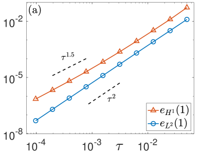
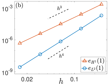
Figure 5.1: $L^{2}$- and $H^{1}$-errors of the sEWI for the NLSE (5.1) with $\sigma=1.1$ and $\alpha=2.51$: (a) temporal errors and (b) spatial errors.

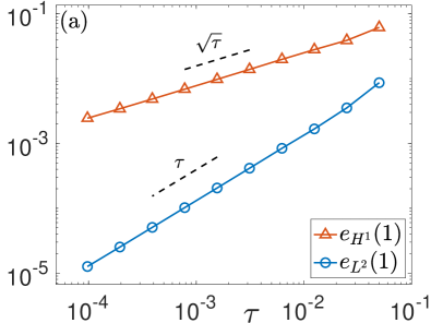
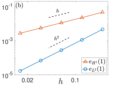
Figure 5.2: $L^{2}$- and $H^{1}$-errors of the sEWI for the NLSE Equation 5.1 with $\sigma=0.1$ and $\alpha=0.51$: (a) temporal errors and (b) spatial errors.

Figures 5.1 and 5.2 plot the errors in $L^{2}$- and $H^{1}$-norm of the sEWI-FS method. We can observe that:

• for "good" nonlinearity with $\sigma=1.1$ and $H^{4}$-initial data, the temporal convergence of the sEWI is second order in $L^{2}$-norm and 1.5 order in $H^{1}$-norm; and the spatial convergence is forth order in $L^{2}$-norm and third order in $H^{1}$-norm;

• for low regularity nonlinearity with $\sigma=0.1$ and $H^{2}$-initial data, the temporal convergence of the sEWI is first order in $L^{2}$-norm and half order in $H^{1}$-norm; and the spatial convergence is second order in $L^{2}$-norm and first order in $H^{1}$-norm.

The numerical results confirm our error estimates in Theorems 3.1, 4.1, 3.2 and 4.2 and show that they are sharp.

Then we consider the NLSE Equation 5.1 with $\sigma=0.5$ and the same $H^{4}$-initial datum with $\alpha=2.51$. Different from the two cases above, we compute the errors of the sEWI-FS with $h=\sqrt{10\tau}$ to satisfy the constraint $\tau\leq h^{2}/(2\pi)$. For comparison, we also plot the errors computed by varying $\tau$ with $h=h_{e}$ fixed (corresponding to the time semi-discrete case).

Figure 5.3 (a) and (b) exhibit errors in $L^{2}$- and $H^{1}$-norm of the sEWI-FS method computed with $h=\sqrt{10\tau}$ and $h=h_{e}$ fixed, respectively. We can observe that, the $L^{2}$-error of the sEWI-FS method is at $O(\tau^{2})$ and the $H^{1}$-error is at $O(\tau^{1.5})$ with and without the time step size restriction $\tau\leq h^{2}/(2\pi)$. The numerical results validate our error estimates in Theorem 4.3, but also suggest that the time step size restriction might be relaxed. We will try to investigate this phenomenon in our future work.

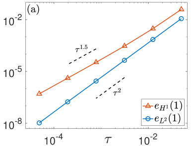
Figure 5.3: $L^{2}$- and $H^{1}$-errors of the sEWI for the NLSE Equation 5.1 with $\sigma=0.5$ and $\sigma=2.51$: (a) errors computed with $h=\sqrt{10\tau}$ and (b) errors computed with $h=h_{e}$ fixed.

Finally, we test the long-time behavior of the sEWI for the NLSE with low regularity nonlinearity. In Figures 5.4 and 5.5, we plot errors of mass and energy up to $T=500$ of the sEWI for the NLSE Equation 5.1 with $\sigma=1.1,\alpha=2.51$ and $\sigma=0.1,\alpha=0.51$, respectively. In both cases, we choose $h=2^{-7}$ fixed and three different $\tau=0.04,0.01,0.0025$. We can observe near conservation of mass and energy over very long time in both cases: the relative error of mass and energy satisfies (based on numerical observation)

$$\frac{|M(\psi^{n})-M(\psi_{0})|}{|M(\psi_{0})|}\leq C_{1}\tau^{2},\quad\frac{|E(\psi^{n})-E(\psi_{0})|}{|E(\psi_{0})|}\leq C_{2}\tau^{2},\quad 0\leq n\tau\leq T=500,$$

where $C_{1}$ and $C_{2}$ seem to be independent of $T$.

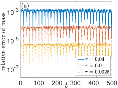
Figure 5.4: Relative errors of (a) mass and (b) energy of the sEWI for the NLSE Equation 5.1 with $\sigma=1.1$ and $\alpha=2.51$.

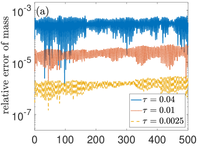
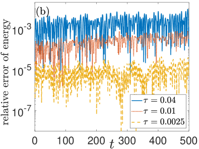
Figure 5.5: Relative errors of (a) mass and (b) energy of the sEWI for the NLSE Equation 5.1 with $\sigma=0.1$ and $\alpha=0.51$.

5.2 For the NLSE with low regularity potential

In this subsection, we consider the NLSE with low regularity potential and cubic (smooth) nonlinearity as

$$i\partial_{t}\psi(\mathbf{x},t) =-\Delta\psi(\mathbf{x},t)+V(\mathbf{x})\psi(\mathbf{x},t)-|\psi(\mathbf{x},t)|^{2}\psi(\mathbf{x},t),\quad\mathbf{x}\in\Omega,\quad t>0,$$ (5.2)

$$\psi(x,0) =\psi_{0}(x),\quad x\in\Omega,$$

where $V$ is chosen as $V_{j}$ with $j=1,2$ defined as

$$V_{1}(x)=\left\{\begin{aligned} &0,&x\in(-4,4)\\ &10,&\text{otherwise}\end{aligned}\right.,\qquad V_{2}(x)=|x|^{1.51}\left(1-\frac{x^{2}}{16^{2}}\right)^{2},\qquad x\in\Omega.$$ (5.3)

Note that the potential functions $V_{1}$ and $V_{2}$ defined in Equation 5.3 satisfy $V_{1}\in L^{\infty}(\Omega)$ and $V_{2}\in H^{2}_{\text{per}}(\Omega)$.

We shall test the convergence orders of the sEWI method for the NLSE Equation 5.2 with $V=V_{j}\ (j=1,2)$ given by Equation 5.3. The "exact" solutions are computed by the sEWI-FS method Equation 2.17 with $\tau=\tau_{\text{e}}:=10^{-5}$ and $h=h_{\text{e}}:=2^{-9}$.

In Figure 5.6, we consider the "good" potential $V=V_{2}\in H^{2}_{\text{per}}(\Omega)$ and an Gaussian initial datum $\psi_{0}(x)=e^{-x^{2}/2}$ in Equation 5.2. In Figures 5.7 and 5.8, we consider the low regularity potential $V=V_{1}\in L^{\infty}(\Omega)$ with an $H^{2}$-initial datum $\psi_{0}(x)=|x|^{1.51}e^{-x^{2}/2}$ and a Gaussian initial data in Equation 5.2, respectively. When computing the temporal errors, we vary $\tau$ with fixed $h=h_{\text{e}}$, and when computing the spatial errors, we vary $h$ with fixed $\tau=\tau_{\text{e}}$.

Figures 5.6, 5.7 and 5.8 plot the errors in $L^{2}$- and $H^{1}$-norm of the sEWI-FS method. We can observe that

• for "good" potential $V\in H^{2}(\Omega)$ and smooth initial data, the temporal convergence of the sEWI is second order in $L^{2}$-norm and 1.5 order in $H^{1}$-norm; and the spatial convergence is forth order in $L^{2}$-norm and third order in $H^{1}$-norm;

• for low regularity potential $V\in L^{\infty}(\Omega)$ and $H^{2}$-initial data, the temporal convergence of the sEWI is first order in $L^{2}$-norm and half order in $H^{1}$-norm; and the spatial convergence is second order in $L^{2}$-norm and first order in $H^{1}$-norm;

• when the $H^{2}$-initial data is replaced with smooth initial data in the case of low regularity $L^{\infty}$-potential, the temporal and spatial convergence shows an increment of half order in both $L^{2}$- and $H^{1}$-norm.

The numerical results in Figures 5.7 and 5.6 validate our error estimates in Theorems 3.1, 4.1, 3.2 and 4.2 and show that they are sharp. The improved spatial convergence rate in Figure 5.8 (b) is due to that the discontinuous potential $V_{1}$ is in $H^{\frac{1}{2}-}(\Omega)$, which roughly leads to an $H^{2.5}$-solution. However, the improved half order temporal convergence rate in Figure 5.8 (a) seems more involved (one can only expect $0.25$ order improvement for $H^{2.5}$-solution), which needs more in-depth analysis and will be left as future work.

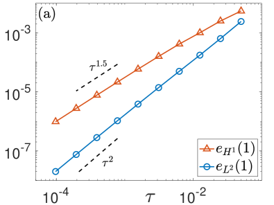
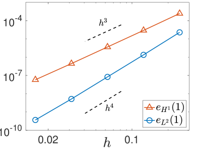
Figure 5.6: $L^{2}$- and $H^{1}$-errors of the sEWI for the NLSE Equation 5.2 with potential $V_{2}$ in Equation 5.3 and an $H^{4}$-initial datum: (a) temporal errors and (b) spatial errors.

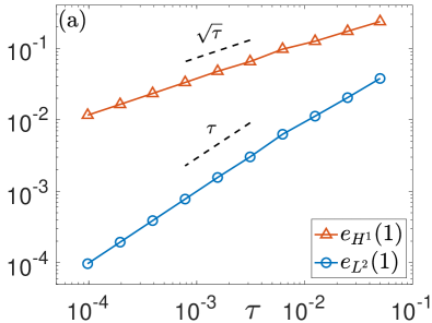
Figure 5.7: $L^{2}$- and $H^{1}$-errors of the sEWI for the NLSE Equation 5.2 with low regularity potential $V=V_{1}$ in Equation 5.3 and an $H^{2}$-initial datum: (a) temporal errors and (b) spatial errors.

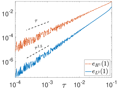
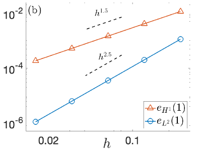
Figure 5.8: $L^{2}$- and $H^{1}$-errors of the sEWI for the NLSE Equation 5.2 with low regularity potential $V=V_{1}$ in Equation 5.3 and a Gaussian initial datum: (a) temporal errors and (b) spatial errors.

As in the previous subsection, we also test the long-time behavior of the sEWI for the NLSE with low regularity potential $V_{1}$ and $V_{2}$. In Figures 5.9 and 5.10, we plot errors of mass and energy up to $T=500$ of the sEWI for the NLSE Equation 5.2 with $V=V_{2},\psi_{0}(x)=e^{-x^{2}/2}$ and $V=V_{1},\psi_{0}(x)=|x|^{1.51}e^{-x^{2}/2}$, respectively. We can observe near conservation of mass and energy over very long time in both cases: the relative error of mass and energy satisfies (based on numerical observation)

$$\frac{|M(\psi^{n})-M(\psi_{0})|}{|M(\psi_{0})|}\leq C_{1}\tau^{2},\quad\frac{|E(\psi^{n})-E(\psi_{0})|}{|E(\psi_{0})|}\leq C_{2}\tau^{2},\quad 0\leq n\tau\leq T=500,$$

where $C_{1}$ and $C_{2}$ seem to be independent of $T$.

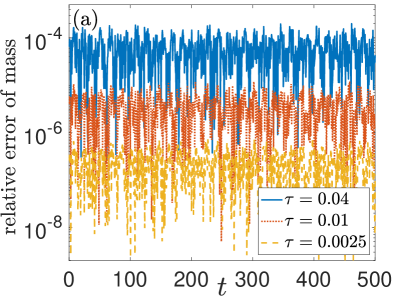
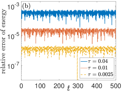
Figure 5.9: Relative errors of (a) mass and (b) energy of the sEWI for the NLSE (5.2) with $V=V_{2}$ and a Gaussian initial datum.

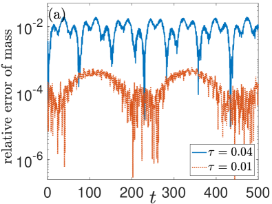
Figure 5.10: Relative errors of (a) mass and (b) energy of the sEWI for the NLSE (5.2) with $V=V_{1}$ and an $H^{2}$-initial datum.

6 Conclusion

We proposed and analyzed a symmetric exponential wave integrator (sEWI) for the nonlinear Schrödinger equation (NLSE) with low regularity potential and nonlinearity. The sEWI is symmetric, explicit and stable under a time step size restriction independent of the mesh size. Moreover, it exhibits excellent performance in solving the NLSE with low regularity potential and/or nonlinearity as well as in the long-time simulation of the NLSE. Rigorous error estimates of the sEWI were established under various regularity assumptions on potential and nonlinearity. Extended numerical results were reported to validate our error estimates and to demonstrate superb long-time behavior of the sEWI.

Acknowledgment. This work was partially supported by the Ministry of Education of Singapore under its AcRF Tier 2 funding MOE-T2EP20122-0002 (A-8000962-00-00).

References

- [1] G. D. Akrivis, Finite difference discretization of the cubic Schrödinger equation, IMA J. Numer. Anal., 13 (1993), pp. 115–124.
- [2] Y. Alama Bronsard, A symmetric low-regularity integrator for the nonlinear Schrödinger equation, 2023, arXiv:2301.13109.
- [3] Y. Alama Bronsard, Error analysis of a class of semi-discrete schemes for solving the Gross-Pitaevskii equation at low regularity, J. Comput. Appl. Math., 418 (2023), pp. 114632.
- [4] Y. Alama Bronsard, Y. Bruned, G. Mainhofer, and K. Schratz, Symmetric resonance based integrators and forest formulae, 2023, arXiv:2305.16737.
- [5] Y. Alama Bronsard, Y. Bruned, and K. Schratz, Low regularity integrators via decorated trees, 2022, arXiv:2211.09402.
- [6] X. Antoine, W. Bao, and C. Besse, Computational methods for the dynamics of the nonlinear Schrödinger/Gross-Pitaevskii equations, Comput. Phys. Commun., 184 (2013), pp. 2621–2633.
- [7] W. Bao and Y. Cai, Mathematical theory and numerical methods for Bose-Einstein condensation, Kinet. Relat. Models, 6 (2013), pp. 1–135.
- [8] W. Bao and Y. Cai, Optimal error estimates of finite difference methods for the Gross-Pitaevskii equation with angular momentum rotation, Math. Comp., 82 (2013), pp. 99–128.
- [9] W. Bao and Y. Cai, Uniform and optimal error estimates of an exponential wave integrator sine pseudospectral method for the nonlinear Schrödinger equation with wave operator, SIAM J. Numer. Anal., 52 (2014), pp. 1103–1127.
- [10] W. Bao, Y. Cai and Y. Feng, Improved uniform error bounds of the time-splitting methods for the long-time (nonlinear) Schrödinger equation, Math. Comp., 92 (2023), pp. 1109–1139.
- [11] W. Bao, Y. Cai and Y. Feng, Improved uniform error bounds on time-splitting methods for long-time dynamics of the nonlinear Klein-Gordon equation with weak nonlinearity, SIAM J. Numer. Anal., 60 (2022), pp. 1962–1984.
- [12] W. Bao, R. Carles, C. Su, and Q. Tang, Error estimates of a regularized finite difference method for the logarithmic Schrödinger equation, SIAM J. Numer. Anal., 57 (2019), pp. 657–680.
- [13] W. Bao, R. Carles, C. Su, and Q. Tang, Regularized numerical methods for the logarithmic Schrödinger equation, Numer. Math., 143 (2019), pp. 461–487.
- [14] W. Bao, R. Carles, C. Su, and Q. Tang, Error estimates of local energy regularization for the logarithmic Schrödinger equation, Math. Models Methods Appl. Sci., 32 (2022), pp. 101–136.
- [15] W. Bao, Y. Feng, and Y. Ma, Regularized numerical methods for the nonlinear Schrödinger equation with singular nonlinearity, East Asian J. Appl. Math., 13(3) (2023), pp. 646-670.
- [16] W. Bao, D. Jaksch, and P. A. Markowich, Numerical solution of the Gross-Pitaevskii equation for Bose-Einstein condensation, J. Comput. Phys., 187 (2003), pp. 318–342.
- [17] W. Bao, Y. Ma, and C. Wang, Optimal error bounds on time-splitting methods for the nonlinear Schrödinger equation with low regularity potential and nonlinearity, 2023, arXiv:2308.15089.
- [18] W. Bao and C. Wang, Error estimates of the time-splitting methods for the nonlinear Schrödinger equation with semi-smooth nonlinearity, Math. Comp. DOI:10.1090/mcom/3900.
- [19] W. Bao and C. Wang, Optimal error bounds on the exponential wave integrator for the nonlinear Schrödinger equation with low regularity potential and nonlinearity, SIAM J. Numer. Anal., to appear (arXiv:2302.09262).
- [20] C. Besse, B. Bidégaray, and S. Descombes, Order estimates in time of splitting methods for the nonlinear Schrödinger equation, SIAM J. Numer. Anal., 40 (2002), pp. 26–40.
- [21] Y. Bruned and K. Schratz, Resonance-based schemes for dispersive equations via decorated trees, Forum Math. Pi, 10, e2 (2022), pp. 1-76.
- [22] R. Carles and C. Su, Scattering and uniform in time error estimates for splitting method in NLS, Found. Comput. Math. DOI:10.1007/s10208-022-09600-9.
- [23] T. Cazenave, Semilinear Schrödinger Equations, volume 10 of Courant Lecture Notes in Mathematics. New York University Courant Institute of Mathematical Sciences, New York, 2003.
- [24] E. Celledoni, D. Cohen, and B. Owren, Symmetric exponential integrators with an application to the cubic Schrödinger equation, Found. Comput. Math., 8 (2008), pp. 303–317.
- [25] W. Choi and Y. Koh, On the splitting method for the nonlinear Schrödinger equation with initial data in , Discrete Contin. Dyn. Syst., 41 (2021), pp. 3837–3867.
- [26] C. Döding, P. Henning and J. Wärnegård, A two level approach for simulating Bose-Einstein condensates by localized orthogonal decomposition, 2022, arXiv:2212.07392.
- [27] J. Eilinghoff, R. Schnaubelt, and K. Schratz, Fractional error estimates of splitting schemes for the nonlinear Schrödinger equation, J. Math. Anal. Appl., 442 (2016), pp. 740–760.
- [28] L. Erdős, B. Schlein, and H.-T. Yau, Derivation of the cubic non-linear Schrödinger equation from quantum dynamics of many-body systems, Invent. Math., 167 (2007), pp. 515–614.
- [29] Y. Feng, G. Maierhofer, and K. Schratz, Long-time error bounds of low-regularity integrators for nonlinear Schrödinger equations, 2023, arXiv: 2302.00383.
- [30] Y. Feng, Z. Xu, and J. Yin, Uniform error bounds of exponential wave integrator methods for the long-time dynamics of the Dirac equation with small potentials, Appl. Numer. Math., 172 (2022), pp. 50–66.
- [31] E. Hairer, C. Lubich, and G. Wanner, Geometric Numerical Integration: Structure-Preserving Algorithms For Ordinary Differential Equations, 2nd ed., Springer, Berlin, 2006.
- [32] P. Henning and D. Peterseim, Crank-Nicolson Galerkin approximations to nonlinear Schrödinger equations with rough potentials, Math. Models Methods Appl. Sci., 27 (2017), pp. 2147–2184.
- [33] M. Hochbruck and A. Ostermann, Exponential integrators, Acta Numer., 19 (2010), pp. 209–286.
- [34] L. I. Ignat, A splitting method for the nonlinear Schrödinger equation, J. Differential Equations, 250 (2011), pp. 3022–3046.
- [35] T. Kato, On nonlinear Schrödinger equations, Ann. Inst. H. Poincaré Phys. Théor., 46 (1987), pp. 113–129.
- [36] M. Knöller, A. Ostermann, and K. Schratz, A Fourier integrator for the cubic nonlinear Schrödinger equation with rough initial data, SIAM J. Numer. Anal., 57 (2019), pp. 1967–1986.
- [37] T. D. Lee, K. Huang, and C. N. Yang, Eigenvalues and eigenfunctions of a Bose system of hard spheres and its low-temperature properties, Phys. Rev., 106 (1957), pp. 1135–1145.
- [38] C. Lubich, On splitting methods for Schrödinger-Poisson and cubic nonlinear Schrödinger equations, Math. Comp., 77 (2008), pp. 2141–2153.
- [39] A. Ostermann, F. Rousset, and K. Schratz, Error estimates at low regularity of splitting schemes for NLS, Math. Comp., 91 (2021), pp. 169–182.
- [40] A. Ostermann, F. Rousset, and K. Schratz, Error estimates of a Fourier integrator for the cubic Schrödinger equation at low regularity, Found. Comput. Math., 21 (2021), pp. 725–765.
- [41] A. Ostermann and K. Schratz, Low regularity exponential-type integrators for semilinear Schrödinger equations, Found. Comput. Math., 18 (2018), pp. 731–755.
- [42] J. Shen, T. Tang, and L.-L. Wang, Spectral Methods: Algorithms, Analysis and Applications, Springer, Heidelberg, 2011.
- [43] C. Sulem and P.-L. Sulem, The Nonlinear Schrödinger Equation: Self-Focusing and Wave Collapse, Springer New York, NY, 1999.
- [44] L. Wang, J. Yan, and X. Zhang, Error analysis of a first-order IMEX scheme for the logarithmic Schrödinger equation, 2023, arXiv: 2306.15901.
- [45] X. Zhao, Numerical integrators for continuous disordered nonlinear Schrödinger equation, J. Sci. Comput., 89 (2021), pp. 40.