The Dependence of Joy’s Law as a Function of Flux Emergence Phase

Abstract

Data from the Michelson Doppler Imager (MDI) and Helioseismic and Magnetic Imager (HMI) are analyzed from 1996 to 2023 to investigate tilt angles ($\gamma$) of bipolar magnetic regions and Joy’s Law for Cycles 23, 24, and a portion of 25. The HMI radial magnetic field ($B_{r}$) and MDI magnetogram ($B_{los}$) data are used to calculate ($\gamma$) using the flux-weighted centroids of the positive and negative polarities. Each AR is only sampled once. The analysis includes only Beta ($\beta$)-class active regions since computing $\gamma$ of complex active regions is less meaningful. During the emergence of the ARs, we find that the average tilt angle ($\bar{\gamma}$) increases from 3.30${}^{\circ}\pm$0.75 when 20% of the flux has emerged to 6.79${}^{\circ}\pm$0.66 when the ARs are at their maximum flux. Cycle 24 had a larger average tilt $\bar{\gamma}_{24}$=6.67$\pm$0.66 than Cycle 23, $\bar{\gamma}_{23}$=5.11$\pm$0.61. There are persistent differences in $\bar{\gamma}$ in the hemispheres with the southern hemisphere having higher ${\bar{\gamma}}$ in Cycles 23 and 24 but the errors are such that these differences are not statistically significant.

1 Introduction

On average, bipolar sunspot pairs are oriented so that the leading sunspot (with respect to rotation) in each hemisphere is closer to the equator than the following sunspot (Hale et al., 1919). This orientation is referred to as the tilt angle and is a measure of the orientation of the bipolar magnetic region’s axis with respect to a line of constant latitude. The tilt angles increase (becoming more North-South oriented and less East-West oriented) with latitude, and this trend was named “Joy’s Law” by Zirin (1988). Different definitions for the zero point and allowed ranges in tilt values exist; a topic discussed this at the end of this section.

Tilt angles are an important aspect of flux-transport dynamo models because the tilt plays a role in the formation and evolution of polar fields [see, e.g., Wang & Sheeley (1991); Dikpati & Charbonneau (1999)]. Tilts serve as an observable feature of the conversion of toroidal magnetic field into poloidal, i.e., the $\alpha$-effect, and the reversal of axial dipole between cycles (Cameron et al., 2018).

There are several proposed physical explanations for the origin of Joy’s law. (Babcock, 1961) proposed that the tilt angle observed in the photosphere reflects the directional components of the global magnetic field at depth and is a direct consequence of the “winding up” of the poloidal field in the solar interior. (Wang & Sheeley, 1991) proposed that Joy’s law is a result of the Coriolis effect acting on flows within the flux tube as it rises through the convection zone. However, a recent study by (Schunker et al., 2020) found the motions of the bipolar magnetic regions were an inherent north-south separation speed of the polarities, independent of flux but dependent on latitude. Their results indicated that the flows in the flux tube need to be directed away from the loop apex if the Coriolis effect were the cause of Joy’s law.

Joy’s law is only obvious after averaging and as such, it is a statistical law. Wang & Sheeley (1989) conducted a study with over 2500 bipolar magnetic regions and reported that 16.6% had no measurable tilts, 19 % were anti-Joy, 4.4 % were anti-Hale. That is 39.9% of regions that did not obey Joy’s law. In another study by McClintock & Norton (2013), the data are so noisy that Joy’s law cannot be recovered for Cycle 17 (Cycle 19) in the northern (southern) hemisphere, respectively. The scatter in the tilt angles is thought to have a physical origin – the buffeting of flux tubes by convective motions (Fisher et al., 1995; Weber et al., 2011). Weaker ARs have higher scatter than stronger ARs (Wang & Sheeley, 1989).

The definition of $\gamma$, data product used for measurement and allowed range of $\gamma$ affect the resultant distribution of measured tilts and any fits to the data. For example, some studies (see Hale et al. (1919); Howard (1991a); Fisher et al. (1995); Dasi-Espuig et al. (2010); McClintock & Norton (2013)) use white-light data without polarity information and a limited range of $\gamma\leq\pm 90^{\circ}$. Under these circumstances, the magnetic polarity is unknown, no anti-Hale angles are possible and therefore many of the recorded $\gamma$ values are incorrect. While data analysis using recorded magnetic field polarities are preferred (see data analysis and results from Wang & Sheeley (1989); Howard (1991b); Norton & Gilman (2005); Li & Ulrich (2012); McClintock et al. (2014); Li (2018); Muñoz-Jaramillo et al. (2021)), white light data catalogs form the longest, most continuous records and allow research on $\gamma$ for many solar cycles.

The frequency of sampling and practice of binning data into latitude bins also affects the results. If all ARs on the disk are sampled multiple times a day or daily, the results are biased to be representative of longer-lived ARs. Sampling the same ARs multiple times (as done by Howard (1991a, b); Fisher et al. (1995); Stenflo & Kosovichev (2012); Dasi-Espuig et al. (2010); McClintock & Norton (2013)) increases the sampling size, thus reducing the standard error of the sample, but this is misleading; if the same AR tilt angle is being recorded multiple times then it is not an independent data point.

Inconsistency in Joy’s law studies are also due to difference practices in fitting. One issue is whether or not the fits are allowed to have a y-intercept or are forced through the origin. The average tilt values near the equator are not zero, indicating that a fit through the origin may not be warranted. Wang & Sheeley (1989); Norton & Gilman (2005); McClintock & Norton (2013); Li (2018) do not force the fit through 0 and Tlatova et al. (2018) states “The presence of an offset in the non-zero tilt at solar equator is a clear indication that the Coriolis force alone cannot explain the active region tilt.”

Another issue is the practice of fitting the averages of data binned in latitude as done by Dasi-Espuig et al. (2010); Stenflo & Kosovichev (2012); McClintock & Norton (2013), as opposed to fitting all the data points at once as done by Li & Ulrich (2012); Li (2018) and this paper. Fitting the binned averages reduces the uncertainty on the returned slope of Joy’s law but may misrepresent the data as the fit gives equal weight to bins containing different numbers of data points.

Analyzing the tilt angles independently by hemisphere is motivated by observations that the northern and southern hemispheres appear to be only moderately to strongly coupled, producing different sunspot numbers and sunspot area (Temmer et al., 2006) in each cycle and having temporal phase shifts for the peak time of the sunspot production and polar field reversals (see Norton et al. (2014) and references therein). Li & Ulrich (2012); McClintock & Norton (2013); Li (2018) report differences in $\bar{\gamma}$ in the northern and southern hemispheres that are statistically significant.

2 Methods

We use magnetic data from MDI (Scherrer et al., 1995) onboard the Solar and Heliospheric Observatory (SOHO) and HMI (Scherrer et al., 2012; Schou et al., 2012) onboard the Solar Dynamics Observatory (SDO) to analyze all beta-type regions during Cycle 23, Cycle 24, and the early stages of Cycle 25. THe Space-weather HMI Active Region Patches (SHARPs) have been identified automatically by Bobra et al. (2014) and for MDI (SMARPs) by Bobra et al. (2021). AR patches that have multiple NOAA (National Oceanic and Atmospheric Administration) numbers are not included in the data set as they are not bipolar and are determined to be too complex to provide meaningful centroid calculations. It is common for ARs to form on the far side and rotate onto the front solar. These regions pose problems for studying the evolution of ARs as there is no way to determine what part of the AR lifetime is being observed. For this reason, AR that did not emerge within 70^∘ of central meridian are not included to ensure that all regions in the data set were observed to emerge on disc.

The location of the leading and following polarities are determined by the flux-weighted-centroids calculated in the MDI and HMI data and $\gamma$ values are defined as the tangent of the change in latitude and longitude between the flux-weighted centroids of the two polarities. $\gamma$ is calculated for a 0-360^∘ range defined with the negative polarity always at the origin and a 0^∘ tilt indicating a completely vertical active region with the negative polarity to the north. Angles increase counter-clockwise. A 90^∘ tilt indicates a completely horizontal AR with a negative leading polarities.

Anti-Hale regions are defined as active regions that don’t obey Hale’s law and therefore have the opposite leading polarity than expected. It is important to note that the tilt angles of anti-Hale regions are computed and recorded within this research but are not used during the fitting of Joy’s law or the determination of the $\bar{gamma}$ values. In Cycle 24, the leading polarity in the northern hemisphere was negative, therefore Hale regions were defined as any region with $\gamma$ between 0–90^∘. Any $\gamma$ in the northern hemisphere (i.e. latitude is $>$0^∘) with a value greater than 180^∘ represented anti-Hale regions and therefore not included in the subsequent Joy’s law fits. Any $\gamma<180$ but $>90$ represented a tilt angle that was anti-Joy, but not anti-Hale, see Figure 1 to visualize the range of $\gamma$ as a function of latitude for ARs in Cycle 24. In Cycle 25, the dominant leading polarity in the northern hemisphere switches to be positive, according to Hale’s law. Therefore all Hale regions in the northern hemisphere had $\gamma$ within the 90-270^∘ range, etc. The Cycle 25 distribution of tilt angles versus latitude was not plotted.

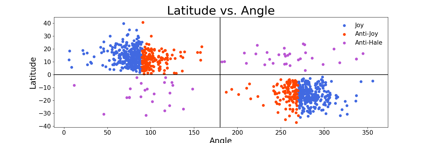
Figure 1: Tilt angle versus latitude for all $\beta$-regions from Cycle 24 with color coding showing Joy, anti-Joy, and anti-Hale regions. All anti-Hale regions are excluded from the data set by defining the northern hemisphere data set as all points in the upper left quadrant and the southern hemisphere data set as all points in the lower right quadrant.

ARs included in our analysis were only sampled once for any given determination of Joy’s law and $\bar{\gamma}$. An AR is sampled at a specific point in time, either when 20% of its flux has emerged, 100% of its flux has emerged, or at the time of central meridian crossing.

To analyze a relationship between size of active region and Joy’s law, total unsigned flux is assumed to be a reasonable indication of the size of the active region. Size thresholds are determined by the median total unsigned magnetic flux ($|\Phi_{median}|$) of all ARs in that hemisphere. Small regions are then defined as ARs whose maximum flux is 0-33% of $|2\Phi_{median}|$. Similarly, medium regions are defined as 33-66% of $|2\Phi_{median}|$ and large regions being defined as those whose flux is greater than 66% of $|2\Phi_{median}|$.

Tilt angles are plotted against latitude and a fit is performed using linear regressions with the form consistent with conventional Joy’s Law fits:

$$\gamma=m_{Joy}\theta+C$$ (1)

where $\gamma$ is the tilt angle, $\theta$ is the latitude, $m_{Joy}$ is the slope, and $C$ is the y-intercept. $C=0$ if the fit is forced through the origin. The best fit is determined using all data points, not data averages binned by latitude which is overplotted on the linear fits to better visualize the data. Only one fit for Joy’s law in Cycle 24 was forced through the origin in order to better compare our results to other studies. All other plots and fits were not forced through the origin. The average tilt angle determined for latitude bins of 5^∘ width is overplotted on the Joy’s law fits for visual purposes only. Error bars on the binned data averages represent the standard error of the mean. The uncertainty of the slope and y-intercept of the fit is also reported.

3 Results

Figure 2 shows the trend of $\gamma$ as a function of latitude from all $\beta$-regions at their maximum unsigned magnetic flux in Cycle 24. The northern (southern) hemisphere tilt values in the 0-360^∘ range were clustered near 90 (270)^∘ for Cycle 24. The black data points connected by the blue line in Figure 2 represent $\gamma$ values averaged in ^∘ latitude bin. The best fit (solid black line) was fit to all of the scatter points in the data set, not just the binned averages shown on the graph. The best linear fit to Cycle 24 data, with both hemispheres combined and the fit forced through the origin, was found to be $\gamma$= 0.44$\theta$, see Figure 2.

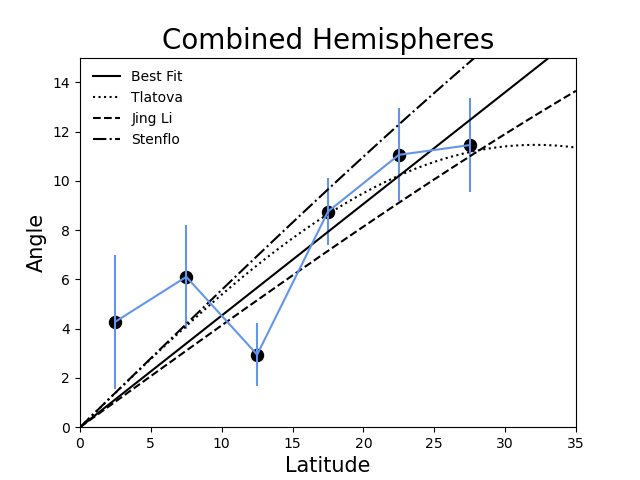
Figure 2: The best fit (solid black line) is fit to all $\gamma$ values for $\beta$-regions in Cycle 24. In order to combine the hemispheres onto a compact graph, the zero point of the tilt angle was changed in each hemisphere such that both hemispheres would have a positive angle increasing with latitude. The equation for the line of best fit, forced through the origin, is $\gamma$ = $0.44\theta$. Overplotted are the data points representing the average $\gamma$ values for Cycle 24 for the northern and southern hemispheres combined for $5^{\circ}$ latitude bins with a blue line connecting the data points. Error bars show the standard deviation of the mean for each bin. Our fit is shown in context with the following results : Tlatova et al. (2018) $\gamma=$ 0.2 sin(2.8$\theta$) (in radians), Li (2018) $\gamma$ = 0.39$\theta$, and Stenflo & Kosovichev (2012) $\gamma$ = 32.1 sin$\theta$. The best fit line plotted here is the only time the line is forced through the origin to better compare our data to other studies that have y-intercepts of zero.

3.1 Fits Separated by Hemisphere

The $\gamma$ of ARs sampled at the time of their maximum (100%) flux are divided into northern and southern hemispheres and analyzed individually in order to observe the differences in activity as shown in Figure 3. In order to overplot both hemispheres onto a compact graph, the zero point of the tilt angle was changed such that both hemispheres would have a positive angle increasing with latitude in accordance with Joy’s law. Linear regressions are used to fit the data with the form $\gamma=m_{Joy}\theta+C$. Linear fits and the overplotted average $\gamma$ values from 5^∘ latitude bins is shown from the northern and southern hemispheres following the procedure detailed earlier with anti-Hale regions being excluded. Results show slightly different linear fits with the lowest latitude bins having distinctly different tilts. Hemispheric fits that were forced through the origin are overplotted with dashed and dotted lines.

The northern hemisphere in Figure 3 shows a clear downturn in the 25-30^∘ band, also observed by Tlatova et al. (2018) and seen in 2. The best fit lines for the two data sets also appear to be different, although these differences cannot be proven to be statistically significant due to the lower sample size after separating the hemispheres, see Table 1 entries for 100% flux for slope ($m_{Joy}$), intercept (C), uncertainties ($\sigma_{m}$ and $\sigma_{C}$), average tilt angle $\bar{\gamma}$ and associated uncertainty ($\sigma_{\bar{\gamma}}$), median tilt angle ($\gamma_{median}$) and number of data points (N). These Cycle 24 Joy’s law parameter entries for 100% flux emerged shown in Table 1 are repeated in Table 2 for Cycle 24.

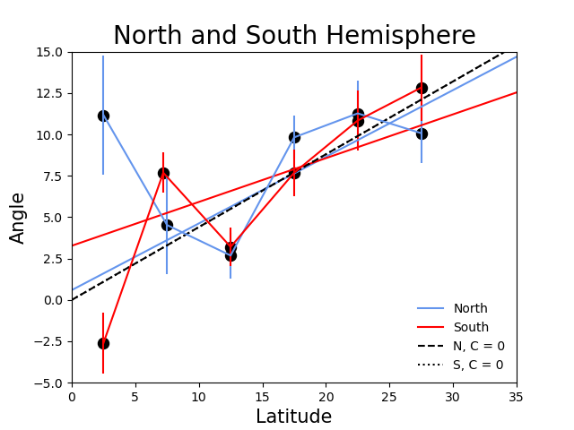
Figure 3: Average tilt angles from Cycle 24 in each hemisphere are shown separately and plotted in $5^{\circ}$ bins. Black dots show these averages connected by blue and red lines for the north and south hemisphere, respectively with error bars calculated as the standard deviation of the mean. Best fit lines are fit to all data points in each data set, not the binned averages. Lines with intercepts are not forced through the origin (red and blue lines) in order to show the true best fit for the data while the lines with intercepts forced through zero (dashed and dotted black lines) are shown for comparison.

3.2 Joy’s Law Dependent On Phase of Emergence

To investigate whether the $\bar{\gamma}$ changes during AR emergence, we sample AR evolution at times when different amount of the maximum unsigned magnetic flux has emerged. Figure 4 plots Joy’s law for of $\beta$-regions in Cycle 24 when 20% and 100% of the maximum unsigned flux for each region has emerged. The hemispheres are separated. Table 2 shows all values and uncertainties associated with fitting Joy’s law as shown in Figure 4.

As seen in Figure 4 in the northern hemisphere, the Joy’s Law slope increases from 0.27 to 0.40 as the unsigned magnetic flux increases. The southern hemisphere shows a reversed trend so the increase or decrease in slope is not consistent and the change in the slope is not statistically significant due to the errors, see $\sigma_{m}$ values in Table 2.

What is significant is that the average tilt angle, $\bar{\gamma}$ increases more than 3^∘ from the time when 20% of the flux has emerged and when 100% of the flux has emerged, see Table 1. This is true in both hemispheres and in the combined hemispheric data.

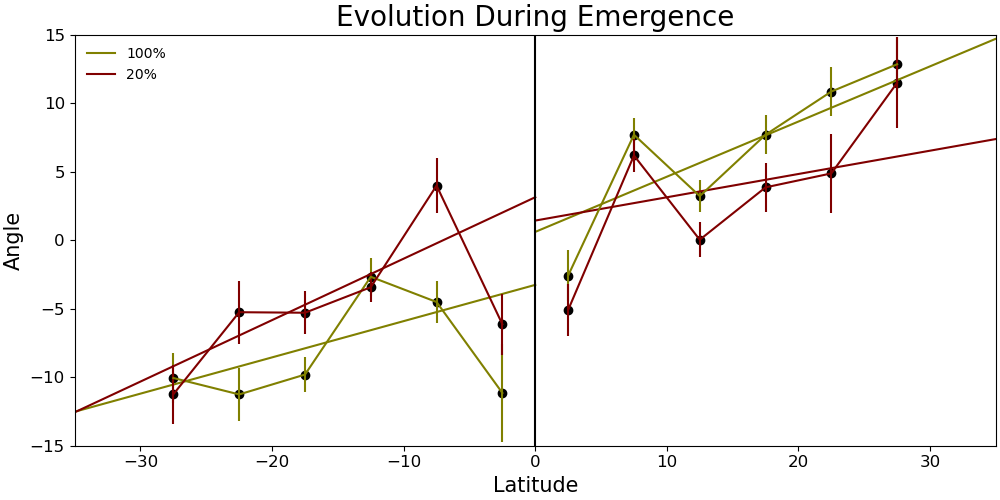
Figure 4: Tilt angles are calculated for all beta regions in Cycle 24 at times when 100% and 20% of their maximum unsigned flux has emerged. The two hemispheres are analyzed separately. Black data points represent average $\gamma$ in $5^{circ}$ latitude bins. Green and brown lines connect the 100% and 20% values, respectively, with error bars representing standard error of the mean for each averaged bin.

Flux Emerged (%)	Hemisphere	$m_{Joy}$	$\sigma_{m}$	C	$\sigma_{C}$	$\bar{\gamma}$	$\sigma_{\bar{\gamma}}$	$\gamma_{median}$	N
100%	North	0.40	0.14	0.59	2.06	6.04	0.90	6.85	480
	South	0.26	0.14	-3.27	2.42	7.42	0.98	6.61	399
	Combined	0.34	0.10	1.68	1.56	6.67	0.66	6.79	879
20%	North	0.27	0.16	-0.89	2.41	2.74	1.05	2.50	426
	South	0.45	0.15	3.12	2.60	4.51	1.06	5.80	369
	Combined	0.36	0.11	-1.97	1.75	3.27	0.75	3.30	795

Table 1: Fits to Joy’s law for tilt angles in Cycle 24 for active regions that have emerged 100% and 20% of maximum flux. The fits are done separately for each hemisphere and then a combined fit is shown. From left to right the columns are the percentage of emerged flux, hemisphere (or combined data from both hemispheres), slope of the Joy’s law fit, uncertainty on the slope, y-intercept, uncertainty of the y-intercept, the average tilt angle, uncertainty of the tilt angle, the median tilt angle, and the number of points in each data set. Uncertainties are calculated as the standard error of the mean.

3.3 Joy’s Law Dependency on Size of AR

AR $\gamma$ values for both Cycle 23 and Cycle 24 are categorized by size and shown as a function of latitude in Figure 5 in different colors for a given size and separated by hemisphere in order to determine if $\gamma$ values and Joy’s law fits were a function of the AR size. Size classifications into small, medium and large regions are made following the procedure detailed in Section 2 using the median of the peak flux values ($\Phi_{median}$) for each hemisphere and cycle. $\Phi_{median}$ of the south and north hemispheres in Cycle 24 was $8.94*10^{21}$ and $9.26*10^{21}$, respectively. $\Phi_{median}$ of the south and north hemispheres in Cycle 23 was $8.51*10^{21}$ and $9.02*10^{21}$, respectively. The average time for the small, medium and large regions to emerge from 20% flux to 100% flux was found to be 2.01, 4.86, and 7.42 days, respectively.

There is no strong correlation between the size of the active regions and the magnitude of their average tilt angles. While the intercepts and slopes vary greatly, they all have large uncertainties due to the high scatter of the data set. We therefore conclude that there is no statistically significant trend and only plot the best fit (separated by hemispheres) line to all data points for Joy’s law for all sizes of ARs, see the black lines in Figure 5. Figure 5 shows the large scatter of the tilt angles of active regions of different sizes in the yellow, green and blue data points representing the small, medium and large ARs.

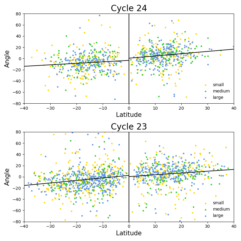
Figure 5: Tilt angles of each active region in Cycles 23 and 24 are plotted at the time of the maximum unsigned flux. Yellow, green, and blue points show results for small, medium and large active regions. The best fit line shown in black is fit to all of the points. We find no significant difference between the best fit lines of different sized active regions and therefore do not show these lines.

3.4 Comparison Between Solar Cycles

In Figure 6, best fit lines for Cycle 23, 24 and the beginning of 25 are shown in the two hemispheres. The northern hemisphere is very consistent and the differences in the slopes and intercepts are statistically insignificant from cycle to cycle. The southern hemisphere is much more variable with significant differences in the slope between Cycle 23 and 24, see the difference between the blue and red lines in the southern hemisphere in Figure 4. The cycle 25 data in incomplete with only 20-30% of the number of data points in the other two cycles. However, the difference in slope between the northern and southern hemispheres in Cycle 25 is quite large even this early in the cycle, see the green line in Figure 4. The fitted parameters and their associated uncertainties are found in Table 2.

The $\bar{\gamma}$ values for the hemisphere-combined data are significantly different between Cycle 23 (5.11^∘ $\pm$ 0.61) and Cycle 24 (6.67^∘ $\pm$ 0.66). The Southern hemisphere contributes most of this difference with $\bar{\gamma}$ values of Cycle 24 being 2.55^∘ higher than those of Cycle 23, see Table 2.

To compare the averages of the hemispheric behavior for the 27 years, all data from the three cycles are combined into two data sets, one for each hemisphere, and a linear regression is fit to both, shown in Figure 7. The southern hemisphere had an overall higher slope and a negative intercept with the northern hemisphere having a smaller slope and positive intercept. Both the northern and southern intercepts, however, are statistically consistent with 0. Comparing these results to other studies reveals similar results within the bounds of uncertainty. The fits to the combined hemispheric data for 27 years can be found in the last two rows of Table 2. We find these results to be in good agreement with Tlatova et al. (2018), Li (2018), and Stenflo & Kosovichev (2012).

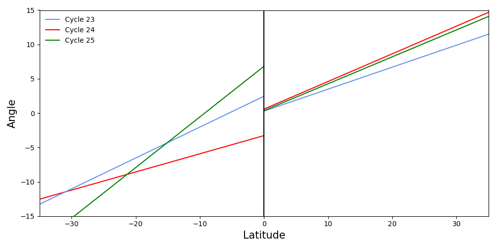
Figure 6: We show best the fit lines for all $\beta$-regions in the northern and southern hemispheres in cycles 23 (blue line), 24 (red line) and early stages of 25 (green line). Lines are fit to all data points in each data set and are not forced through the origin.

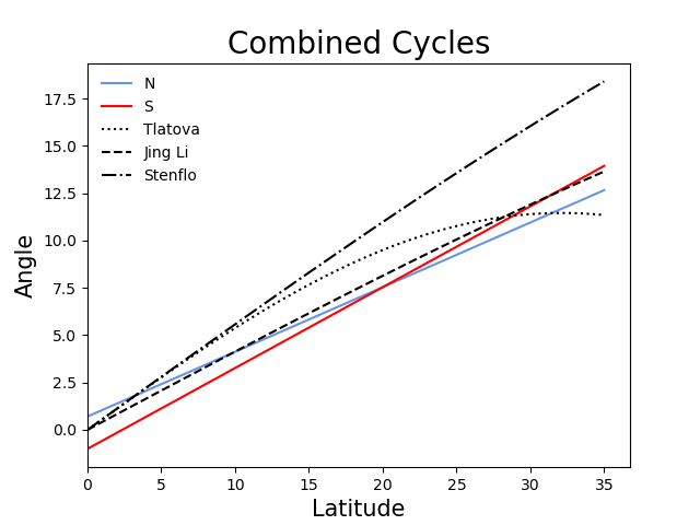
Figure 7: We show the best fit line for all $\beta$-regions in each hemisphere for the combined cycles 23, 24, and the beginning of cycle 25. The best fit lines are not forced through the origin, however it is worth noting that the intercepts are very small compared to those from fits for each separate cycle.

Cycle	Hemisphere	$m_{Joy}$	$\sigma_{m}$	C	$\sigma_{C}$	$\bar{\gamma}$	$\sigma_{\bar{\gamma}}$	$\gamma_{median}$	N
Cycle 25	North	0.39	0.26	0.37	5.16	7.80	1.56	10.33	150
	South	0.74	0.17	-6.83	3.63	8.19	1.31	8.41	154
	Combined	0.60	0.15	-3.80	3.04	8.00	1.02	9.49	304
Cycle 24	North	0.40	0.14	0.59	2.06	6.04	0.90	6.85	480
	South	0.26	0.14	-3.27	2.42	7.42	0.98	6.61	399
	Combined	0.34	0.10	1.68	1.56	6.67	0.66	6.79	879
Cycle 23	North	0.32	0.11	0.30	1.93	5.41	0.88	7.00	593
	South	0.45	0.10	-2.14	1.80	4.87	0.83	6.36	763
	Combined	0.39	0.07	-1.26	1.32	5.11	0.61	6.68	1356
Combined Cycles	North	0.34	0.08	0.70	1.33	5.95	0.59	7.28	1223
	South	0.43	0.07	-1.19	1.34	6.05	0.59	6.96	1316

Table 2: Fits to Joy’s law for tilt angles for Cycles 23, 24, and 25. The fits are done separately for each hemisphere and then a combined fit is shown. From left to right the columns are the percentage of emerged flux, hemisphere (or combined data from both hemispheres), slope of the Joy’s law fit, uncertainty on the slope, y-intercept, uncertainty of the y-intercept, the average tilt angle, uncertainty of the tilt angle, the median tilt angle, and the number of points in each data set. Uncertainties are calculated as the standard error of the mean.

3.5 Significance of Sampling Time

Tilt angles measured at the time of maximum flux of each active region and from the time of central meridian crossing are compared to determine if there is a significant difference in the average tilt angles or Joy’s law fit that depends on the sampling. The data from central meridian crossing was taken from the SPEAR (Solar Photospheric and Ephemeral Active Region) catalogue.

Figure 8 shows the average 5^∘ bins for the data points from both data sets separated by hemisphere and the linear fit done to all data points (not the binned data). There is not a significant difference in the linear regression slopes and intercepts in the data from the northern hemisphere and in the intercepts from the southern hemisphere, see Table 3. The $\bar{\gamma}$ values resulting from sampling at the time of maximum flux and central meridian are also statistically the same.

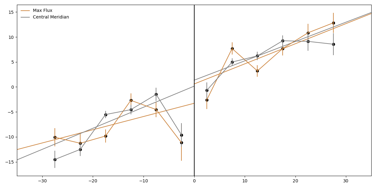
Figure 8: Comparison of Joy’s Law in Cycle 24 determined by sampling the ARs at the time of maximum flux versus the central meridian crossing. Best fit lines are fit to all $\beta$ regions and are not forced through the origin and fit to all $\beta$-type regions. Overlaid points represent average $\gamma$ values from 5^∘ bins in latitude.

Time Measured	Hemisphere	$m_{Joy}$	$\sigma_{m}$	C	$\sigma_{C}$	$\bar{\gamma}$	$\sigma_{\bar{\gamma}}$	$\gamma_{median}$	N
Maximum Flux	North	0.40	0.14	0.59	2.06	6.04	0.90	6.85	480
	South	0.26	0.14	-3.27	2.42	7.42	0.98	6.61	399
	Combined	0.34	0.10	1.68	1.56	6.67	0.66	6.79	879
Central Meridian	North	0.39	0.12	1.35	1.71	6.56	0.70	6.47	741
	South	0.42	0.11	-0.15	1.96	6.81	0.67	7.11	709
	Combined	0.38	0.08	0.94	1.26	6.68	0.48	6.77	1450

Table 3: The parameters of the best fit line for Joy’s law for tilt angles in Cycle 24 as sampled at their maximum unsigned flux and at their central meridian crossing times. Values for the Maximum Flux rows are the same values seen in Table 1 in the 100% row and the meanings of the parameters from left to right were described for previous tables.

4 Discussion

Joy’s law is a statistical law and the large scatter means that the results are sensitive to sample size and choices in fitting techniques. If ARs are only sampled once and the hemispheres are separated, it is difficult to find a statistical different between the slopes and intercept of Joy’s law, especially in Cycle 24 as the number of data points are on the order of 400-500.

Our best linear fit when fitting Cycle 24 data with both hemispheres combined and forcing the fit through the origin is $\gamma$=0.44$\theta$, see Figure  2. This is consistent with Li (2018) reporting the best fit to be $\gamma=(0.39\pm 0.06)\theta-(0.66\pm 1.00)$ and other fits to data that contain magnetic polarity information. Notably, a similar downturn is observed in the HMI data that is also observed by (Tlatova et al., 2018), indicating that active regions at latitudes higher than the 25-30^∘ bin do not increase monotonically. Since $\gamma$ does not increases monotonically for latitudes higher than 25^∘, the form of Joy’s law proposed by Tlatova et al. (2018) $\gamma=0.2sin(2.8\theta)$ is sensible.

The fits shown in 3 emphasize the difference between forcing the linear regressions through the origin and allowing the fits to have a y-intercept. Many other studies including Stenflo & Kosovichev (2012), Li (2018) and Tlatova et al. (2018) plotted Joy’s Law fits with linear regressions forced through the origin under the assumption that, logically, tilt angles at the equator should be 0^∘. However, in doing so, there is some information that is lost in the process. When forcing the best fits through the origin (black and grey dotted line), they both have the same slope. This would lead to the conclusion that the two hemispheres are completely symmetrical, as assumed by Stenflo & Kosovichev (2012) and many others. However, when plotting the linear regressions without forcing the lines through the origin (blue and red), they have different slopes and different intercepts. While these slopes are not statistically significant due to the large scatter in the data, we suggest that these results indicate a possible difference in hemispheric activity.

An interesting feature reported by Tlatova et al. (2018) is that at 0^∘ latitude, odd cycles have positive offsets and even cycles have negative offsets up through cycle 22. We did not observe a similar effect although the difference may be due to differences in fitting: Tlatova et al. (2018) fit the latitudinally binned data that contained multiple entried for a given AR while our procedure only samples an AR once and fits all data points, not the binned averages. However, this may be an interesting point for further investigation, especially if one can concentrate only on the lower latitude ARs that appear to be the regions contributing to the offset.

The statistically significant result that the $\bar{\gamma}$ values in the combined hemispheric data increase from 3.27$\pm$0.75^∘ when 20% of the flux has emerged in an AR to 6.67$\pm$0.66^∘ (see Table 1 confirms previous results of Schunker et al. (2020) who found that ARs initially emerge nearly East-West aligned and the tilt angles become larger, on average, as more flux emerges. The individual hemispheres exhibit the same trend with an approximately 3^∘ increase in $\bar{\gamma}$ values during emergence. Stenflo & Kosovichev (2012) also finds an evolution towards the standard Joy’s law tilt over the course of an AR lifetime.

Previous research has reported that $\gamma$ and Joy’s law slopes are not dependent on the amount of flux contained within the AR or the size of the AR (Fisher et al., 1995; Stenflo & Kosovichev, 2012). The attempt to distinguish a tilt or Joy’s law dependency on size of ARs in MDI and HMI also led to a null result.

The $\bar{\gamma}$ values being higher for Cycle 24 (6.67^∘ $\pm$ 0.66) as compared to Cycle 23 (5.11^∘ $\pm$ 0.61) fits into the theory that tilt angles are a feedback mechanism to limit the runaway growth of a solar cycle (Jiang, 2020), and that there is a trend that a weak cycle will produce a larger tilt angle than a strong cycle (Dasi-Espuig et al., 2010).

Regarding the result that Joy’s law fits are similar for data sampled at the time of AR maximum flux versus the time of central meridian crossing (see Table 3 and Figure 8), we suggest that the high scatter of the data helps to reduce the error in measuring $\gamma$ at central meridian. The central meridian sampled data does not take into account what stage of development the active region is in, therefore it can be assumed that it is sampling regions at all stages of emergence and decay.

A relatively recently studied feature of ARs that may be influential in the determination of $\gamma$ is the “ magnetic tongue”. At the very early stage of emergence, the twist of the magnetic field on the flux tube may influence the measured tilt angle as the azimuthal component of the field is projected onto the vertical, see Poisson et al. (2016) research on magnetic tongues (or tails). Preliminary studies show that identifying and removing these magnetic tongues from the AR data prior to calculating the tilt angle may lower the scatter in the values (Poisson et al., 2020).

HMI and MDI have provided an abundance of magnetic field data of solar ARs for the past 27 years. Tilt angles and Joy’s law have been studied using this data, as well as data that have come before these, but as yet, the community doesn’t agree as to the underlying mechanism that imparts the tilts. However, increasingly detailed and creative studies are being conducted and with them, hope for more clarity as to the role that the Coriolis effect plays versus other mechanisms that may impart AR tilt angles.

References

- Babcock (1961) Babcock, H. W. 1961, ApJ, 133, 572, doi: 10.1086/147060
- Bobra et al. (2014) Bobra, M. G., Sun, X., Hoeksema, J. T., et al. 2014, Sol. Phys., 289, 3549, doi: 10.1007/s11207-014-0529-3
- Bobra et al. (2021) Bobra, M. G., Wright, P. J., Sun, X., & Turmon, M. J. 2021, ApJS, 256, 26, doi: 10.3847/1538-4365/ac1f1d
- Cameron et al. (2018) Cameron, R. H., Duvall, T. L., Schüssler, M., & Schunker, H. 2018, A&A, 609, A56, doi: 10.1051/0004-6361/201731481
- Dasi-Espuig et al. (2010) Dasi-Espuig, M., Solanki, S. K., Krivova, N. A., Cameron, R., & Peñuela, T. 2010, A&A, 518, A7, doi: 10.1051/0004-6361/201014301
- Dikpati & Charbonneau (1999) Dikpati, M., & Charbonneau, P. 1999, ApJ, 518, 508, doi: 10.1086/307269
- Fisher et al. (1995) Fisher, G. H., Fan, Y., & Howard, R. F. 1995, ApJ, 438, 463, doi: 10.1086/175090
- Hale et al. (1919) Hale, G. E., Ellerman, F., Nicholson, S. B., & Joy, A. H. 1919, ApJ, 49, 153, doi: 10.1086/142452
- Howard (1991a) Howard, R. F. 1991a, Sol. Phys., 136, 251, doi: 10.1007/BF00146534
- Howard (1991b) —. 1991b, Sol. Phys., 132, 49, doi: 10.1007/BF00159129
- Jiang (2020) Jiang, J. 2020, ApJ, 900, 19, doi: 10.3847/1538-4357/abaa4b
- Li (2018) Li, J. 2018, ApJ, 867, 89, doi: 10.3847/1538-4357/aae31a
- Li & Ulrich (2012) Li, J., & Ulrich, R. K. 2012, ApJ, 758, 115, doi: 10.1088/0004-637X/758/2/115
- McClintock & Norton (2013) McClintock, B. H., & Norton, A. A. 2013, Sol. Phys., 287, 215, doi: 10.1007/s11207-013-0338-0
- McClintock et al. (2014) McClintock, B. H., Norton, A. A., & Li, J. 2014, ApJ, 797, 130, doi: 10.1088/0004-637X/797/2/130
- Muñoz-Jaramillo et al. (2021) Muñoz-Jaramillo, A., Navarrete, B., & Campusano, L. E. 2021, ApJ, 920, 31, doi: 10.3847/1538-4357/ac133b
- Norton et al. (2014) Norton, A. A., Charbonneau, P., & Passos, D. 2014, Space Sci. Rev., 186, 251, doi: 10.1007/s11214-014-0100-4
- Norton & Gilman (2005) Norton, A. A., & Gilman, P. A. 2005, ApJ, 630, 1194, doi: 10.1086/431961
- Poisson et al. (2016) Poisson, M., Démoulin, P., López Fuentes, M., & Mandrini, C. H. 2016, Sol. Phys., 291, 1625, doi: 10.1007/s11207-016-0926-x
- Poisson et al. (2020) Poisson, M., López Fuentes, M. C., Mandrini, C. H., Démoulin, P., & MacCormack, C. 2020, A&A, 633, A151, doi: 10.1051/0004-6361/201936924
- Scherrer et al. (1995) Scherrer, P. H., Bogart, R. S., Bush, R. I., et al. 1995, Sol. Phys., 162, 129, doi: 10.1007/BF00733429
- Scherrer et al. (2012) Scherrer, P. H., Schou, J., Bush, R. I., et al. 2012, Sol. Phys., 275, 207, doi: 10.1007/s11207-011-9834-2
- Schou et al. (2012) Schou, J., Borrero, J. M., Norton, A. A., et al. 2012, Sol. Phys., 275, 327, doi: 10.1007/s11207-010-9639-8
- Schunker et al. (2020) Schunker, H., Baumgartner, C., Birch, A. C., et al. 2020, A&A, 640, A116, doi: 10.1051/0004-6361/201937322
- Stenflo & Kosovichev (2012) Stenflo, J. O., & Kosovichev, A. G. 2012, ApJ, 745, 129, doi: 10.1088/0004-637X/745/2/129
- Temmer et al. (2006) Temmer, M., Rybák, J., Bendík, P., et al. 2006, A&A, 447, 735, doi: 10.1051/0004-6361:20054060
- Tlatova et al. (2018) Tlatova, K., Tlatov, A., Pevtsov, A., et al. 2018, Sol. Phys., 293, 118, doi: 10.1007/s11207-018-1337-y
- Wang & Sheeley (1989) Wang, Y. M., & Sheeley, N. R., J. 1989, Sol. Phys., 124, 81, doi: 10.1007/BF00146521
- Wang & Sheeley (1991) —. 1991, ApJ, 375, 761, doi: 10.1086/170240
- Weber et al. (2011) Weber, M. A., Fan, Y., & Miesch, M. S. 2011, ApJ, 741, 11, doi: 10.1088/0004-637X/741/1/11
- Zirin (1988) Zirin, H. 1988, Astrophysics of the sun (”Cambridge University Press”)