Refined Equivalent Pinhole Model for Large-scale 3D Reconstruction from Spaceborne CCD Imagery

Abstract

In this study, we present a large-scale earth surface reconstruction pipeline for linear-array charge-coupled device (CCD) satellite imagery. While mainstream satellite image-based reconstruction approaches perform exceptionally well, the rational functional model (RFM) is subject to several limitations. For example, the RFM has no rigorous physical interpretation and differs significantly from the pinhole imaging model; hence, it cannot be directly applied to learning-based 3D reconstruction networks and to more novel reconstruction pipelines in computer vision. Hence, in this study, we introduce a method in which the RFM is equivalent to the pinhole camera model (PCM), meaning that the internal and external parameters of the pinhole camera are used instead of the rational polynomial coefficient parameters. We then derive an error formula for this equivalent pinhole model for the first time, demonstrating the influence of the image size on the accuracy of the reconstruction. In addition, we propose a polynomial image refinement model that minimizes equivalent errors via the least squares method. The experiments were conducted using four image datasets: WHU-TLC, DFC2019, ISPRS-ZY3, and GF7. The results demonstrated that the reconstruction accuracy was proportional to the image size. Our polynomial image refinement model significantly enhanced the accuracy and completeness of the reconstruction, and achieved more significant improvements for larger-scale images.

1 Introduction

Numerous sources are available for producing digital surface models (DSMs), including UAV, aerial, and satellite imagery, and point data can be obtained from laser scanner. Despite there exist the large amount of source utilized to obtain DSMs, extracting DSM results from satellite images is the most cost-effective option given the constant influx of terabyte-scale image data. Since satellites with various high-resolution (VHR) sensors, such as the WorldView-3 and Gaofen-7 series, were first launched, optical satellite images have achieved a resolution of better than 1 m. VHR satellite imagery has the potential to enhance the precision of DSM reconstruction and facilitate the 3D reconstruction of urban areas Poullis (2020); Bosch et al. (2017); Stucker et al. (2022).

Large-scale reconstruction of the earth’s surface from satellite images for the purpose of obtaining complete and accurate DSM results remains a challenge. Typically, a linear-array pushbroom is used to acquire satellite imagery, and a generalized rational functional model (RFM) Tao and Hu (2000, 2001) is used for the imaging equation. Hence, pinhole camera images differ significantly from the imaging methods and imaging equations of linear array charge-coupled device (CCD) images. However, traditional methods for 3D reconstruction de Franchis et al. (2014a); Bosch et al. (2016); Michel et al. (2020) of optical satellite images often rely on RFM. The 3D reconstruction of satellite optical images based on RFM involves several essential steps, such as bundle adjustment Tang and Tan (2019); Marí et al. (2019), epipolar rectification de Franchis et al. (2014b); Tatar and Arefi (2019); Liao et al. (2022), dense matching Zhang et al. (2019a); Xia et al. (2020), point cloud generation Gong and Fritsch (2018), and DSM fusion filtering Wang and Frahm (2017); Gómez et al. (2023). Many studies have focused on improving these steps.

Additionally, numerous commercial software packages (e.g., ERDAS Imagine LPS Leica (2023), RSP Qin (2016), MicMac Rupnik et al. (2017), Pixel Factory Factory (2023), SURE nFrames (2023), SOCET SET BAESystem (2023), Agisoft Metashape Agisoft (2023), and Catalyst professional Catalyst (2023)) and open source pipelines (e.g., S2P de Franchis et al. (2014a), CARS Michel et al. (2020), and ASP Beyer et al. (2018)) have been developed to photogrammetrically process satellite images using RFM. ERDAS Imagine LPS (Leica Photogrammetry Suite) Leica (2023) is a well-established and robust photogrammetric processing package for aerial and orbital imagery. Nearly every orbital sensor is supported by rigorous information describing the camera model. For most other sensors, rational polynomial coefficient (RPC) processing is also supported. Pixel Factory Factory (2023) generates 3D mesh models from satellite images. By using multiple images for each model, it is able to process very large areas. One feature exclusive to Pixel Factory is that homogeneity and consistency are guaranteed throughout the world. SURE Software nFrames (2023) transforms imagery from classic aerial cameras, multi-head oblique systems, drone cameras, and most consumer-grade terrestrial cameras into 2.5D or 3D data, including point clouds, photorealistic textured meshes, and true orthophotos, via a streamlined fully automatic and integrated image processing technique. MinMac Rupnik et al. (2017) is free open-source photogrammetric software for 3D reconstruction, and it solved the multi-view fusion with a multi-directional dynamic programming technique for dense matching of VHR satellite images (Rupnik et al., 2017, 2018). S2P de Franchis et al. (2014a) is a fully automated modular pipeline designed for affine reconstruction of line-array satellite images. Furthermore, the NASA Ames Research Center proposed the NASA Ames Stereo Pipeline Beyer et al. (2018), which is a suite of free and open-source automated geodesy and stereogrammetry tools for processing stereo images captured from satellites, in which rigorous physical sensor models are obtained by querying ephemerides and interpolating camera poses.

The fully automatic and modular stereo pipeline S2P de Franchis et al. (2014a) utilizes an affine model in the image space to optimize positioning based on PRC model. Facciolo et al. (2017) proposed a method that relies on local affine approximation Grodecki and Dial (2003) and considers multi-date images, making it a multi-modal technique for reconstructing 3D models. Michel et al. (2020) designed a new scalable, robust, high-performance stereo pipeline for satellite images called CARS. Wang et al. (2022) proposed a hierarchical reconstruction framework that consists of an affine dense reconstruction stage and an affine-to-Euclidean upgrading stage based on multiple optical satellite images, which needs only four ground control points (GCPs). To attain a simple and speedy dense matching outcome, the 3D reconstruction pipelines detailed above execute stereo correction before the dense matching stage. However, it is difficult to accurately stereo-correct large-scale satellite stereo image pairs Liao et al. (2022); Tatar and Arefi (2019); de Franchis et al. (2014b); Jannati et al. (2018) because spaceborne optical sensors always follow the linear-array pushbroom imaging process, during which there are differences between the epipolar geometries of different linear-array images. Most importantly, the imaging model for linear-array CCD images is complicated and relies on a generic RPC model fitted with polynomials, which introduces difficulties in constraining the reconstruction results with the original rigorous imaging model. Zhang et al. (2019b) proposed the Adapted COLMAP to fit the RFM to the pinhole camera model (PCM), which fundamentally solves the problem of relying on RFM for linear-array CCD images. After resolving the disparity between the imaging models of linear array CCDs and pinhole cameras, ZhangKai et al. successfully accomplished 3D reconstruction of line-array CCD images utilizing the first-rate open-source computer vision software, COLMAP.

To this end, in this study we propose the RFM is equivalent to PCM (REPM) pipeline, which is based on the Adapted CLOMAP pipeline Zhang et al. (2019b) and relies heavily on the idea of RFM is equivalent to PCM to expand its applicability to linear-array CCD imagery. To enhance the reconstruction accuracy of the REPM pipeline, we construct a image refinement model that minimizes equivalent errors. We also incorporate an image-partitioning module and improve the DSM fusion module by enabling it to process large-scale images. In summary, our main contributions are as follows:

• We introduce the RFM is equivalent to PCM model and mathematically derive the error formula of the equivalent pinhole model, which enables large-scale 3D reconstruction with linear array imagery using most exisiting 3D reconstruction pipelines. In addition, we further propose the image refinement model to improve the accuracy of 3D reconstruction.

• We present a multi-view 3D reconstruction pipeline for large-scale linear-array CCD imagery based on REPM, which encompasses the whole process from image intake to DSM product output.

• We have proven through formula derivation and experiments that the error of the equivalent pinhole model is directly proportional to the image size. Additionally, our pipeline shows excellent potential on four datasets. Remarkably, incorporating a polynomial image refinement model highlights a 15% accuracy advancement on large surface format images.

2 Methods for 3D reconstruction method of satellite images

In this section, we focus on three satellite image-based 3D reconstruction methods: RFM-based, PCM-based, and REPM-based 3D reconstruction.

2.1 RFM-based 3D reconstruction

Satellite images are commonly captured by using linear-array CCD sensors in a pushbroom manner, the projection method of which is significantly different from that of the traditional pinhole camera model. Most satellite optical images reconstruct DSMs through the RPC models, which include 80 polynomial coefficients (78 polynomial coefficients to be solved) and 10 normalized constants (for a total of 90 parameters in the RPC file corresponding to each image), which are defined as

$$\left\{\begin{matrix}u=\mu_{u}+\sigma_{u}g(\frac{lat-\mu_{lat}}{\sigma_{lat}},\frac{lon-\mu_{lon}}{\sigma_{lon}},\frac{alt-\mu_{alt}}{\sigma_{alt}})\\ v=\mu_{v}+\sigma_{v}h(\frac{lat-\mu_{lat}}{\sigma_{lat}},\frac{lon-\mu_{lon}}{\sigma_{lon}},\frac{alt-\mu_{alt}}{\sigma_{alt}})\end{matrix}\right.,$$ (1)

where $u,v$ represent the row and column pixel coordinates, respectively; $lat,lon,alt$ denote the latitudes, longitudes, and altitudes of the locations within the WGS-84 coordinate system, respectively; $\mu_{i}(i=u,v,lat,lon,alt)$ denotes five translation normalization parameters; $\sigma_{i}(i=u,v,lat,lon,alt)$ denotes five scaling normalization parameters; and the functions $g(\cdot)$ and $h(\cdot)$ are the cubic polynomial functions of the RPC model, each with 40 parameters. Because the numerators and denominators of the $g(\cdot)$ functions are simultaneously divided by a polynomial coefficient, the ratio remains unchanged. The same applies to the $h(\cdot)$ functions. Therefore, out of the 80 polynomial coefficients, there are two constant values of 1.

The traditional RFM-based 3D reconstruction method Tao and Hu (2002) involves initially acquiring the transformation between image pairs with homologous points using matching techniques. Then a 3D model of the reconstructed ground information is derived by accounting for various coordinate standardization parameters based on the RFM of stereo image pairs. However, the complexity of the RFM renders the entire reconstruction process extremely cumbersome. The S2P pipeline de Franchis et al. (2014a) offers a solution for decoupling the 3D reconstruction process from the intricacies of satellite imaging. The S2P pipeline utilizes the relative pointing error correction between RPC models to replace the complicated nonlinear bundle adjustment. This process recovers the 3D structure of the paired satellite images using a simple RPC-based elevation iteration. Michel et al. (2020) presented a new stable and efficient pipeline for multi-view stereo called CARS. In this pipeline, a colocalization function that employs the epipolar constraint, is fitted with a geometry based on a nonrigid iterative approximation. Then it jointly and recursively estimates two resampling grids mapped from the estimated epipolar geometry to the input images. Wang et al. (2022) proposed a hierarchical reconstruction framework based on multiple optical satellite images called AE-Rec, which reconstructs the affine and Euclidean scene structures sequentially. In the first stage, an affine dense reconstruction approach is used to obtain the 3D affine structure from the input satellite images, and local small-sized tiles in the satellite images are approximately subject to an affine camera model. This affine approach is performed under an incremental reconstruction strategy and does not use any GCP. In the second stage, the obtained 3D affine structure is upgraded to a Euclidean structure by fitting a global transformation matrix with at least four GCPs.

2.2 PCM-based 3D reconstruction

Most 3D reconstructions based on the PCM adopt the idea that the overlapping image first performs feature point matching. The matched feature points are then used to obtain the ground point coordinates via space resection. However, because of the diversity of constraints, it is difficult to unify many 3D reconstruction methods. For example, 3D reconstruction based on local stereo matching Loghman and Kim (2013); Bleyer et al. (2011) uses the consistency of parallax in a small range for constraints, 3D reconstruction based on global stereo matching Felzenszwalb and Huttenlocher (2004) explicitly uses smooth assumption constraints to solve the matching results of all pixels as a whole, and 3D reconstruction based on semiglobal stereo matching Hirschmuller (2005) uses mutual information as the method for computing the similarity measure. Additional priori knowledge can be used as constraints to improve the accuracy of the 3D reconstruction.

Furthermore, the combination of structure from motion (SfM) Schönberger and Frahm (2016) and multi-view stereo (MVS) Schönberger et al. (2016) is considered a favorable vision-based reconstruction framework for 3D scene restoration. SfM estimates the camera position, orientation and reconstructs the sparse point clouds. Subsequently, MVS generates dense point clouds based on the SfM results to reconstruct the 3D scene. However, the linear-array CCD images do not rigorous constraints of camera position and orientation like pinhole camera images because of the significant differences between the imaging models of pinhole cameras and those of satellite linear-array sensors. Thus, this framework primarily focuses on the 3D reconstruction of images captured using pinhole cameras.

2.3 REPM-based 3D reconstruction

Statistical analyses in the literature Zhao et al. (2023) show that traditional 3D reconstruction methods are still significant in the field of 3D reconstruction of satellite images. However, these satellite-based 3D reconstruction methods rely on RFM. Because of the RPC function’s complexity, incompatibility with many novel 3D reconstruction pipelines, and lack of a rigorous epipolar correction model, a recent innovative approach suggested fitting the RFM to the PCM. The Adapted COLMAP Zhang et al. (2019b) method approximates a weak perspective projection model using a well-established RFM and enhances the original COLMAP Schönberger and Frahm (2016); Schönberger et al. (2016) visual reconstruction pipeline for satellite images with a depth reparameterization technique, thereby improving the accuracy of the depth values. However, the Adapted COLMAP method is only applicable to small-scale images. In this pipeline, the equivalent error is larger for large-scale images, the reconstruction effect is poorer, and NOT AVAILABLE (NA) even occurs. To reduce the equivalent error, we corrected image using polynomial function, which is called the image refinement model. In addition, to address the NA phenomenon in large-scale images, we added an image partition module and improved the DSM generation module.

3 REPM-based 3D reconstruction pipeline

This section presents the REPM pipeline framework, the algorithmic and error formulas of the equivalent pinhole model, and the principle of the image refinement model. The design of the REPM pipeline includes the RPC model’s approximation of the pinhole camera model, image refinement model and relies heavily on features included in Adapted COLMAP Zhang et al. (2019b), including the SfM Schönberger and Frahm (2016) and MVS Schönberger et al. (2016) frameworks.

3.1 REPM pipeline

An overview of the reconstruction process is presented in Fig.1. Under the assumption of weak perspective projection, the REPM pipeline performs multi-view image processing by using $n$ source images and their RPC parameters to compute the internal matrix, rotation matrix, and translation vectors $\{\mathbf{K}_{i},\mathbf{R}_{i},\mathbf{t}_{i}\}_{i=0}^{N}$ corresponding to the input views through the equivalent pinhole model. The corrected image is then obtained using a image refinement model that minimizes the error of the equivalent pinhole model. The SfM framework performs sparse reconstruction with the given $\{\mathbf{K}_{i},\mathbf{R}_{i},\mathbf{t}_{i}\}_{i=0}^{N}$ and corrected images. The sparse point cloud and optimized camera poses jointly participate in the MVS phase to estimate the depth map, and then fuse to generate the dense point cloud and DSM.

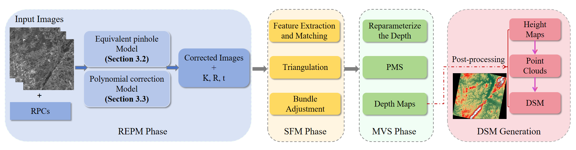
Figure 1: Overview of the reconstruction process of the REPM pipeline. The procedure involves four phases: REPM, SfM, MVS, and DSM generation. The inputs consist of several overlapping images and their corresponding RPC models. The outputs include height maps, georeferenced 3D point clouds, and digital surface models.

REPM phase. In the REPM phase, we introduce the RFM is equivalent to PCM algorithm and implement a image refinement model to rectify the image by minimizing the equivalent error. We first perform image partitioning and image enhancement operations, in which the accuracy of the equivalent pinhole model is influenced by the size of the satellite image and the equivalent error is decreased by clipping the image. Image enhancement is necessary because the long-tail distribution of the brightness values of the satellite image is detrimental to image feature matching. We set a brightness threshold and perform the image enhancement technique when the brightness values exceed this threshold. After image partitioning and enhancement, the images and RPC parameters are fed into the equivalent pinhole model described in Section 3.2 and the image refinement model described in Section 3.3.

SfM and MVS phases. For the SfM and MVS phases, we employ the same approach as that used in Adapted COLMAP Zhang et al. (2019b). In the field of computer vision, the SfM and MVS frameworks are well-developed 3D reconstruction frameworks, which are used in the excellent reconstruction pipeline COLMAP. During the SfM stage, feature extraction and matching are initially performed to match the homonymous points of the stereo image. Next, triangulation is conducted to calculate the 3D point coordinates from the homonymous points. Finally, global optimization is executed using beam method leveling to generate an optimal camera parameter model. SfM produces the internal parameters, position, sparse point cloud, and co-visual relationship of the point cloud. Using this information, MVS executes pixel-by-pixel dense matching to create a depth map that matches the corresponding source images. In addition, to address the issue of inaccuracy caused by large depth values, the reparameterization approach is adopted and then the depth map is estimated using the classical PatchMatch Stereo (PMS) Bleyer et al. (2011) algorithm.

DSMs aggregation. We restructured the DSM generation model to align it with the processing of the image partition module. Because the image is partitioned into multiple image tiles, the reconstructed DSMs from the same viewpoint are first mosaicked, and then DSMs from different perspectives are aggregated. Because the image-matching process does not guarantee 100% accuracy, the reconstructed DSM results contain incorrect height values. Therefore, outlier removal is incorporated into the process of aggregating DSMs, including two methods: 1) the median absolute deviation (MAD), which is used to filter out DSM outliers, and 2) radius point cloud filtering, which removes noise. However, a disadvantage of radius point cloud filtering is the absence of a standard parameter, which necessitates combining the reconstruction results to determine the parameter.

3.2 Equivalent pinhole model

3.2.1 Introduction to the equivalent pinhole model

The equivalent pinhole model is based on the principle of weak perspective projection. First, let the range of the ground altitude variation be denoted by $Z_{range}$ and the distance from the satellite sensor to the ground point be denoted by the depth $D$. For remote sensing images, the satellite sensor is far from the ground point (i.e., $D\gg Z_{range}$). In this case, the average scene depth can be used in the projection calculation instead of the depth; this substitution is the theoretical basis for approximating the perspective camera as a weak perspective camera. Furthermore, Zhang et al. (2019b) proved that a linear pushbroom camera can be reduced to a weak perspective camera under the same conditions. Therefore, a linear pushbroom camera can be approximated as a perspective camera, which we refer to as the equivalent pinhole model. The procedure of the equivalent pinhole model algorithm is presented in Algorithm 1. Given the RPC parameters of the images, the projection matrix of the perspective camera model (i.e., the internal matrix $K$ and the external matrices $R$ and $t$) can be estimated using the equivalent pinhole model algorithm.

Algorithm 1: Equivalent Pinhole Model Algorithm.

Input: RPC parameters

Output: K, R, t parameters

1: Calculate the latitude, longitude, and altitude ranges based on the RPC parameters, and construct a set of hierarchical virtual 3D target grid points based on the range.

$X\_min=X_{off}-X_{scale}$

$X\_max=X_{off}+X_{scale}$

$(X=Latitude,Longitude,Altitude)$

$(Lat,Lon,Alt)_{n}$

2: Project the 3D points onto the image utilizing the RPC parameter, and filter out correspondences with pixel coordinates that lie outside the image boundary.

$(Row,Col)=F(Lat,Lon,Alt);$

$mask=(Row<0,Row>height,Col<0,Col>width)$

3: Convert the 3D points from the WGS-84 coordinate system to the ENU coordinate system.

$(Lat,Lon,Alt)_{n}\longrightarrow(e,n,u)_{n}$

4: Calculate the projection matrix P from 3D point coordinates to 2D pixel coordinates is solved using singular value decomposition (SVD).

$SVD(e,n,u,Row,Col)\longrightarrow P$

5: The factorization projection matrix P forms K, R, t for the camera’s intrinsic and extrinsic parameters.

$P\longrightarrow K,R,t$

3.2.2 Error formula of the equivalent pinhole model

The equivalent pinhole model algorithm equates the RPC parameters of the RFM with the internal and external parameters of the PCM via

$$\begin{split}&\binom{u}{v}=F(lat,lon,alt)\Rightarrow\\ &Z_{cam}\begin{pmatrix}u\\ v\\ 1\end{pmatrix}=P_{3\times 4}\begin{pmatrix}X\\ Y\\ Z\\ 1\end{pmatrix}=K_{3\times 3}\left[R|t\right]_{3\times 4}\begin{pmatrix}X\\ Y\\ Z\\ 1\end{pmatrix}\end{split},$$ (2)

where $F(\cdot)$ denotes the cubic polynomial function of the RPC model; $u,v$ denote the pixel coordinates’ columns and rows, respectively; $lat,lon,alt$ indicate the latitude, longitude, and altitude, respectively, in the WGS-84 coordinate system; $\begin{pmatrix}u&v&1\end{pmatrix}^{T}$ is the homogeneous coordinate in the pixel coordinate system; $\begin{pmatrix}X&Y&Z&1\end{pmatrix}^{T}$ is the homogeneous coordinate in the east-north-up (ENU) coordinate system; $Z_{cam}$ denotes the $Z$-coordinate of the object point in the camera coordinate system (which can also be interpreted as the depth value of the object point); $P_{3\times 4}$ is the projection matrix that converts the object point coordinates into pixel coordinates; and $K,R,t$ are obtained by factorizing the projection matrix $P$.

Both the RFM and PCM are utilized to model the relationship between 2D pixel coordinates and 3D object point coordinates. The RFM uses a cubic polynomial function, which is computationally complex. In contrast, the PCM employs homogeneous coordinates and matrix multiplication, which significantly simplify operations such as rotation and translation in 3D space. The RFM and PCM use different world coordinate systems, and the equivalent pinhole model algorithm utilizes the ENU coordinate system because of its relative compatibility with the conventional PCM (compared to the WGS-84 coordinate system).

The weak perspective projection principle is utilized to approximate a linear pushbroom camera as a perspective camera. Accordingly, a weak perspective projection formula is used to derive the equivalent error formula. The weak perspective projection formula is

$$\left\{\begin{matrix}x=\frac{f_{x}{X_{cam}}}{\bar{Z}}\\ \\ y=\frac{f_{y}{Y_{cam}}}{\bar{Z}}\end{matrix}\right.,$$ (3)

where $x,y$ are the image coordinates that are projected onto the object point coordinates within the image-space coordinate system; $f_{x},f_{y}$ represent the mapping of the sensor focal length on the $x$ and $y$ axes, respectively; $(X_{cam},$ $Y_{cam},Z_{cam})$ denote the object point coordinates in the image space coordinate system; and $\bar{Z}$ denotes the average value of all object points within the image area.

We consider the perspective projection formula for the x-axis as an example for further derivation. For digital images, the multiple-order derivatives of the perspective projection formula can be obtained; thus, the formula satisfies the conditions for Taylor expansion. Because we approximate the projection model as a weak perspective projection and $Z_{cam}$ is approximated as $\bar{Z}$, we obtain the Taylor expansion at $\bar{Z}$:

$$\begin{split}x&=\frac{f_{x}X_{cam}}{Z_{cam}}\\ &=\frac{f_{x}X_{cam}}{\bar{Z}}+\frac{{x}^{\prime}(\bar{Z})}{1!}(Z_{cam}-\bar{Z})+o(Z_{cam}-\bar{Z})^{2}\end{split},$$ (4)

where $o(\cdot)$ is the Peano remainder term of the Taylor expansion, representing the higher order infinitesimals of (a-b).

Next, by comparison with Eq.(3), we obtain an error formula approximated as a weak perspective projection:

$$E=\frac{{x}^{\prime}(\bar{Z})}{1!}(Z_{cam}-\bar{Z})=-f_{x}\frac{X_{cam}}{\bar{Z}^{2}}(Z_{cam}-\bar{Z}).$$ (5)

The higher-order term of the Taylor formula was not considered.

The factors that influence the equivalent error can be derived from Eq.(5). As $f_{x}\frac{X_{cam}}{\bar{Z}}\approx x$, we can derive $\left|E\right|\approx\left|-x(Z_{cam}-\bar{Z})/\bar{Z}\right|$. Ideally, when reconstructing the 3D information of a particular area, a schematic such as that shown in Fig.2 should be drawn to assist with the illustration. As $Z_{cam}\gg Z_{cam}-Z_{min}$ and $\bar{Z}=(Z_{max}+Z_{min})/2$, we propose that $\bar{Z}$ is similar in image regions $A$ and $B$. Consequently, we demonstrate that in identical spatial areas, the equivalent error is determined by the image size and the disparity in ground elevation $Z_{cam}-\bar{Z}$. For images $A$ and $B$, $E_{A}\leq\left|-x_{A}(Z_{A}^{max}-\bar{Z})/\bar{Z}\right|$, $E_{B}\leq\left|-x_{B}(Z_{B}^{max}-\bar{Z})/\bar{Z}\right|$. Because $u_{A}>u_{B}$ and $Z_{A}^{max}>Z_{B}^{max}$, we conclude that $E_{A}>E_{B}$. Based on Fig.2, it can be inferred that, in general, the size of an image can indirectly determine the height difference between the ground and the corresponding object, which is proportional to the size of the image. Therefore, to control the equivalent error in the experiments, suitable image sizes were routinely obtained via cropping.

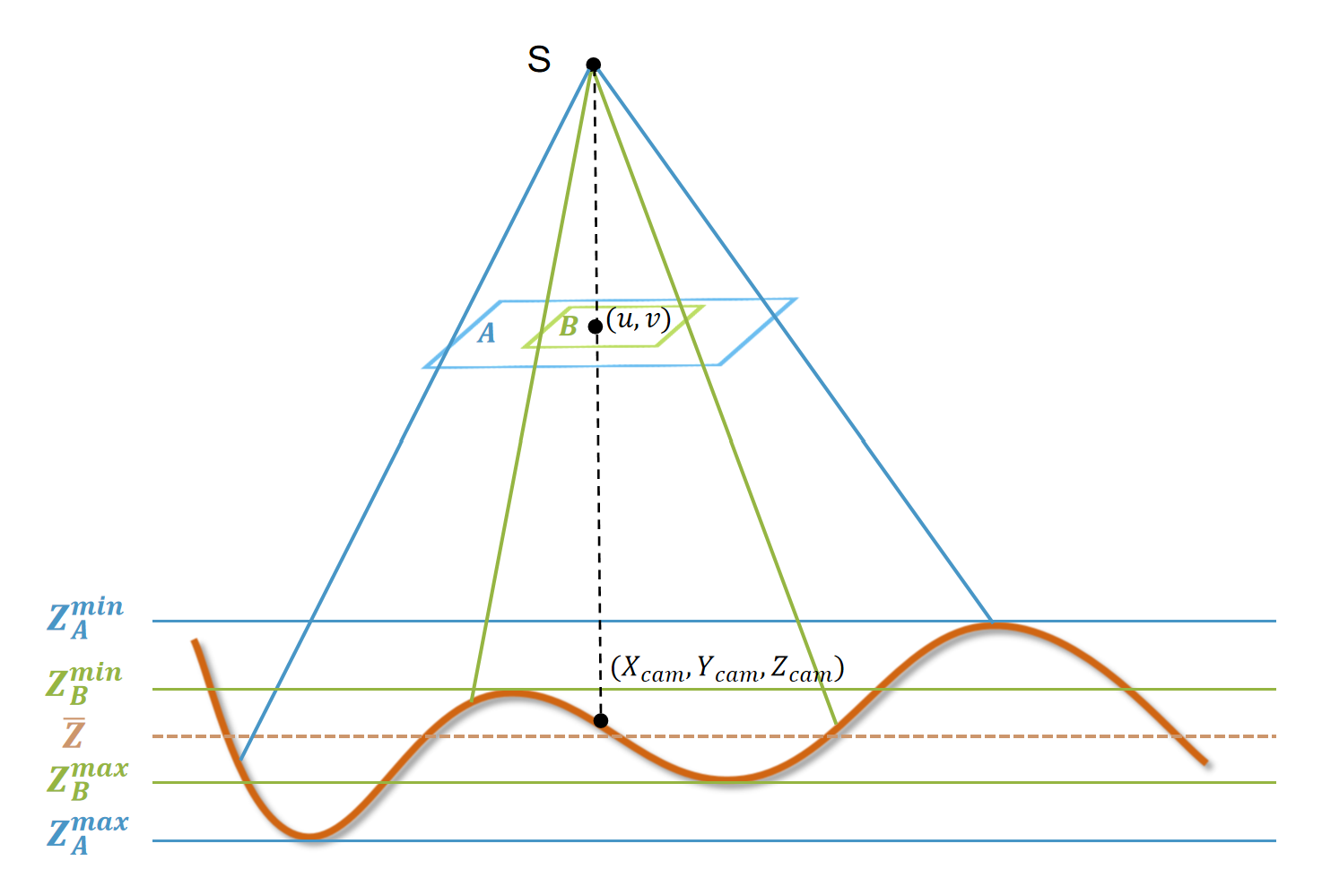
Figure 2: Diagram of the error formula of equivalent model. The brown region represents the earth’s surface, and the blue and green regions represent the projection of images A and B for two different image sizes, respectively, for the same surface on the earth.

3.3 Image refinement model

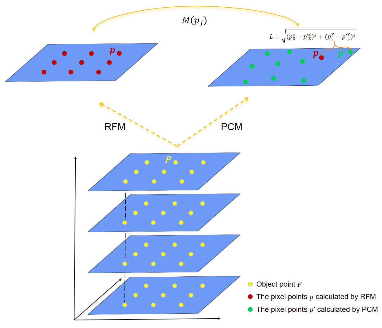
Figure 3: Image refinement model. An object point $P$ is taken as an example, and $p$ and ${p}^{\prime}$ denote the positions before and after correction, respectively.

In Section 3.2.2, we explained that the error in the equivalent pinhole model arises from using RFM and PCM to calculate the positional deviation from the object point to the pixel point. To reduce this bias, we minimize the equivalent error by introducing a polynomial image refinement model, as shown in Fig.3. The pixel points calculated via the RFM and PCM form $n$ sets of corresponding points, which are substituted into the polynomial correction function:

$$\begin{cases}x^{\prime}=m_{0}+m_{1}x+m_{2}y+m_{3}xy+m_{4}x^{2}+m_{5}y^{2}\\ y^{\prime}=m_{6}+m_{7}x+m_{8}y+m_{9}xy+m_{10}x^{2}+m_{11}y^{2}\end{cases},$$ (6)

where $m_{i}(i=0,1\cdots 11)$ are the coefficients of the polynomial function.

The parameters of the polynomial image refinement model are computed using the least squares method:

$$\underset{M(p)}{min}\sum_{j}\left\|M(p_{j})-{p}^{\prime}_{j}\right\|_{2}^{2}.$$ (7)

Finally, the polynomial image refinement model is used to resample the original image to obtain the corrected image.

Initially, our aim was to correct the image by minimizing the equivalent error through the homography transformation. However, the results of the homography correction model were unsatisfactory. Instead, we selected a more complex second-order polynomial transformation to correct the images and reduce the equivalent pinhole model error. Through experiments, we found that the polynomial correction was more effective (see Section 5.3 for a description of the experiments). Therefore, we added the polynomial image refinement model before starting the downstream reconstruction task. The algorithm used for correcting the model is presented in Algorithm 2.

Algorithm 2: Image refinement Model Algorithm.

Input: Original images; RPC parameters; and $K,R,t$ parameters

Output: Corrected images and the polynomial image refinement function $M(\cdot)$

1: From Algorithm 1, hierarchical virtual 3D target grid points are projected through the RFM imaging model to produce $n$ sets of 3D-2D ($P$, $p$) correspondences.

$P(X,Y,Z)_{n}\longrightarrow p(x,y)_{n}$

2: The hierarchical virtual 3D target grid points are projected to obtain pixels $p^{\prime}$ based on the equivalent PCM imaging model, where $p$ and $p^{\prime}$ constitute the $n$ sets of corresponding points.

$P(X,Y,Z)_{n}\longrightarrow{p}^{\prime}({x}^{\prime},{y}^{\prime})_{n}$

$(x,y,{x}^{\prime},{y}^{\prime})_{n}$

3: We back-calculate the polynomial parameters to correct the image. The relationship between $p$ and ${p}^{\prime}$ is used to calculate the polynomial iamge refinement parameters via the least squares method.

$\underset{M(p^{\prime})}{min}\sum_{j}\left\|M(p^{\prime}_{j})-{p}_{j}\right\|_{2}^{2}$

4: After polynomial correction, the corrected image is generated. The polynomial correction function $M(\cdot)$ is used to compute the pixel positions of the original image, and the bilinear interpolation step in the resampling process provides the digital number (DN) values of the corrected image.

$DN({p_{j}}^{\prime})=DN(M(p^{\prime}_{j}))$

3.4 Reconstruction of the DSM

A major factor that distinguishes satellite stereo pipelines from typical vision pipelines is the camera model (RPC vs. pinhole). Once we have obtained the corrected images and the internal and external parameter matrices of the equivalent pinhole camera, we can feed them into the SfM and MVS frameworks in the Adapted COLMAP pipeline Zhang et al. (2019b) to reconstruct the 3D information. The goal of SfM is to recover accurate camera parameters for use in subsequent MVS steps. In addition, the authors identified and resolved key issues in the MVS framework that prevented the direct application of standard MVS pipelines tailored for ground-level images to the satellite domain.

4 Experiments

In this section, we describe the datasets we used and the experiments we conducted on them. We also present an analysis of the experimental results.

4.1 Experimental setup

4.1.1 Datasets

We assessed our pipeline using three publicly accessible image datasets: the WHU-TLC test set, the DFC2019 dataset, and the ISPRS-ZY3 image data. We also present the reconstruction outcomes of applying the REPM pipeline to GF7 image data.

• WHU-TLC test set. The WHU-TLC test set, including three-view images and RPC parameters that have been refined in advance to achieve sub-pixel reprojection accuracy, is provided by Gao et al. (2021). The ground-truth DSMs were prepared using both high-accuracy LiDAR observations and GCP-supported photogrammetric software. The DSM is stored as a regular grid with 5-m resolution using the WGS-84 geodetic coordinate system and the UTM projection coordinate system.

• DFC2019 dataset. The four sites of the DFC2019 dataset Bosch et al. (2019) from the 2019 IEEE Geoscience and Remote Sensing Society (GRSS) Data Fusion Competition were used in this study. The dataset was obtained using the WorldView3 satellites. The dataset is comprised of satellite images featuring multiple views captured on multiple dates between 2014 and 2016. Each RGB image measures $2048\times 2048$ pixels, and the ground truth DSM is $512\times 512$ pixels.

• ISPRS-ZY3 data. China’s first high-resolution stereo mapping civilian satellite, ZY3, has provided reliable high-resolution stereo image data. The experimental data from the International Society for Photogrammetry and Remote Sensing (ISPRS-ZY3) ISPRS (2018) covers Sainte-Maxime, France, including three line-array stereo panchromatic images of 2.1 m for nadir and 2.5 m for forward and backward. The ISPRS-ZY3 data consists of 12 ground control points for checking the absolute accuracy of the DSM.

• GF7 data. The Gaofen-7 (GF7) satellite has a dual-line array stereo camera that delivers high-precision remote sensing imagery with a panchromatic stereo resolution superior to 0.8 m, with 0.8 m for forward and 0.64 m for backward. Our experimental findings revealed an area in Zhengzhou, China with an image size measuring $35864\times 40000$ pixels. Furthermore, a local reference DSM measuring $5717\times 6043$ pixels is available as a benchmark in comparison experiments.

4.1.2 Implementation details

The experiments were conducted in a computing environment featuring an NVIDIA A100-PCI graphics card with a video memory of 40 GB. Python was used as the programming language, and VCcode served as the compiler. Four distinct 3D reconstruction methods were employed for experimental testing, and the implementation details are provided below.

S2P. Satellite Stereo Pipeline (S2P) is an automatic and modular stereo pipeline for pushbroom images. The images are divided into small tiles and processed in parallel using multiple processes to improve efficiency. In our experiment, the tile size was set to 500-1000 pixels, and the dense matching method in S2P was the default More Global Matching (MGM) algorithm Facciolo et al. (2015). In the fusion step, an outlier removal threshold of 25 m was chosen (the same operation as in Gao et al. (2023)), and the height map outlier cleaning was set to false (otherwise, the completeness rate was meager). The other settings were left at their default values.

LPS. The Leica Photogrammetry Suite (LPS) Leica (2023) is a collection of digital software for processing photogrammetry and remote sensing data. The software performs binocular stereo reconstruction, thereby displaying the outcomes with maximum precision when using multi-view images as input.

Adapted COLMAP. Adapted COLMAP (AC) Zhang et al. (2019b) fits the pinhole camera model to the image-based RPC model, and then employs a computer vision reconstruction pipeline for 3D reconstruction. However, Adapted COLMAP cannot handle large-scale images, and the direct output of large-scale images is displayed as NA. Therefore, the pipeline was only run on the WHU TLC and DFC2019 datasets.

Sat-MVSF.

Ours. We used our REPM pipeline to reconstruct the DSM for two datasets, the WHU-TLC and DFC2019 dataset, which are referred to as “Ours” in the experiments. In addition, the REPM pipeline was constructed based on the Adapted COLMAP, which we improved by incorporating the image partition module. We also improved the DSM generation module to reconstruct the DSM, which is referred to as “REPM” in the experiments. When the image refinement model is introduced, it is called “REPM+Ref.” in the experiments. The crop size represents both length and width in all experiments.

4.1.3 Accuracy metrics

We utilized the assessment metric codes established in the literature Zhang et al. (2019b), and the equations employed to calculate the assessment metrics are as follows.

(1) The root-mean-square error (RMSE), which is the standard deviation of the residuals between the ground truth and the estimation, is defined as

$$RMSE=\sqrt{\frac{(\hat{h}_{i}-h_{i})^{2}}{N_{i}}}(i\in(\hat{h}\cap h)),$$ (8)

where $\hat{h},h$ denote the predicted and true values, respectively, and $N_{x}$ denotes the number of computations required. For example, when calculating the RMSE accuracy of the reconstructed DSM, $\hat{h},h$ denote the heights of the generated DSM and true DSM, respectively, and $N_{i}$ denotes the number of pixels.

(2) The median error (ME), which is the median of the absolute values of the residuals between the ground truth and the estimation, is defined as

$$ME=median\left|\hat{h}_{i}-h_{i}\right|(i\in(\hat{h}\cap h)).$$ (9)

(3) The mean absolute error (MAE), which is the mean of the absolute values of the residuals between the ground truth and the estimation, is defined as

$$MAE=\frac{1}{n}\left(\sum_{i=1}^{n}\left|\hat{h}_{i}-h_{i}\right|\right)(i\in(\hat{h}\cap h)).$$ (10)

(4) Completeness, which is the percentage of points with a height error less than a certain threshold. In this study, the completeness is denoted as $Comp_{threshold}$ and defined as

$$Comp_{threshold}=\frac{N_{\left|\hat{h}_{i}-h_{i}\right|<threshold}}{N_{i}}(i\in h).$$ (11)

(5) Time consumption, which is the time that elapses between the input of an image and the generation of a DSM product. The unit of time is min.

4.2 Comparative results on benchmark datasets

We evaluated the proposed pipeline on four datasets, and compared its performance to the experimental results obtained from the image reconstruction pipeline for classic linear-array satellite CCDs de Franchis et al. (2014a) and from commercial software Leica (2023).

4.2.1 Results for the WHU-TLC test set

To evaluate the accuracy and completeness of our proposed reconstruction pipeline, we compared its performance to that of other reconstruction methods using the WHU-TLC test set. To ensure fairness, we used more straightforward point-cloud filtering for postprocessing. Table 1 compares the experimental results for the WHU-TLC test set contained in the literature Gao et al. (2023) to our results. The table shows that our method outperformed other methods in terms of accuracy and completeness and that there was no significant decrease in the running time of our method. Furthermore, compared to the Adapted COLMAP approach, the addition of our image refinement model led to a 5.52% increase in the RMSE accuracy and a 2.57% improvement in the completeness for a threshold of 2.5 m.

Table 1 shows that our method improves both the accuracy and completeness. The poor RMSE accuracy of LPS can be attributed to the WHU-TLC test set, which is comprised of 46 image sets, some of which are occluded by clouds, whereas others have weakly textured regions such as water bodies. Because of LPS’s inability to densely match such regions, a triangulation mesh is used to fill in the gaps, and the DSM outliers cannot be removed by point-cloud filtering, eventually resulting in an overall poor RMSE accuracy.

Table 1: Quantitative results of DSM reconstruction quality on the WHU-TLC test set. (Bold works best)

Methods	MAE(m)$\downarrow$	RMSE(m)$\downarrow$	Comp2.5(%)$\uparrow$	Comp5(%)$\uparrow$	Time(min.)$\downarrow$
CATALYST* Gao et al. (2023)	3.454	7.939	52.31	82.52	3.80
Metashape* Gao et al. (2023)	2.693	13.047	56.59	75.46	24.51
SDRDIS * Gao et al. (2023)	4.496	15.012	47.58	73.57	9.41
Sat-MVSF * Gao et al. (2023)	1.895	3.654	64.82	80.05	5.87
S2P	1.692	8.710	66.738	94.652	7.487
LPS	3.581	13.934	62.242	91.729	8.062
AC	1.766	3.334	73.926	97.428	7.171
Ours	1.666	3.150	75.826	97.308	7.317

• This is from the results of qualitative experiments on the WHU-TLC test set in Gao et al. (2023). The time of Sat-MVSF represents inference time and does not include training time.

A comparison between the DSM reconstruction output and the error maps for the WHU test set is shown in Fig. 4. S2P had more pixels with reconstruction failures than LPS, and all the pixels from LPS were successfully reconstructed. This discrepancy may be attributed to the provision of a low-resolution digital elevation model (DEM) by the ERDAS LPS software. A comparison of the error maps demonstrates that the iamge refinement model significantly enhanced the reconstruction accuracy and that our method had the highest reconstruction accuracy.

image1

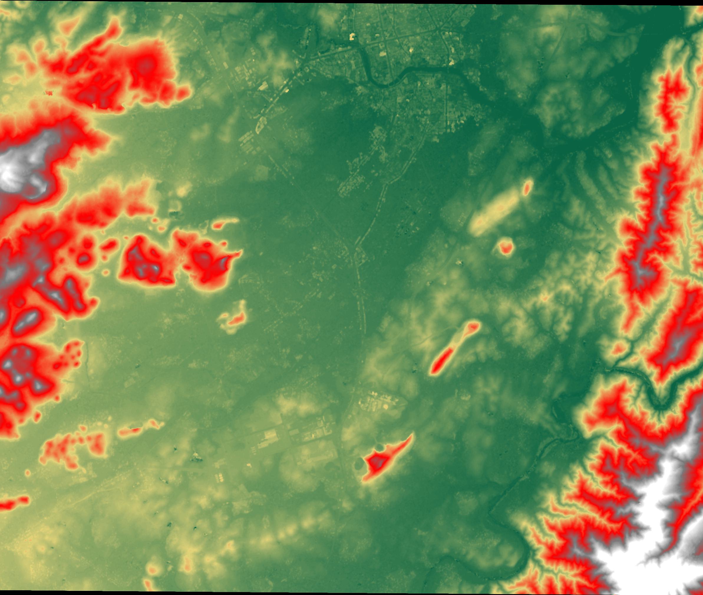
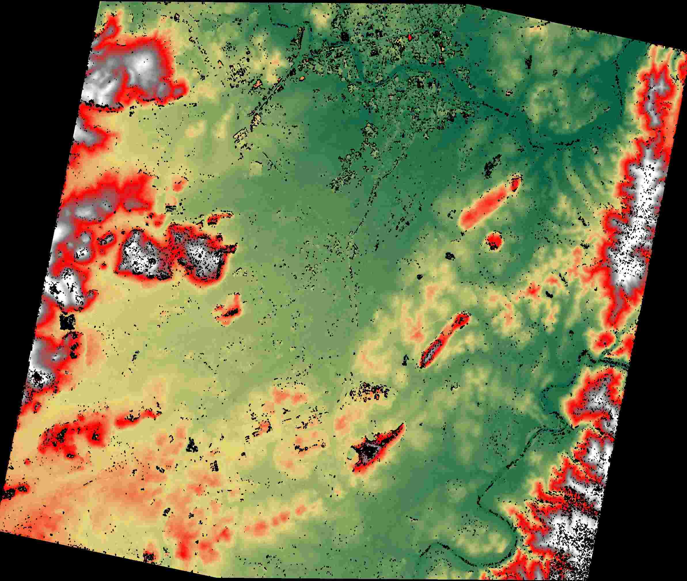
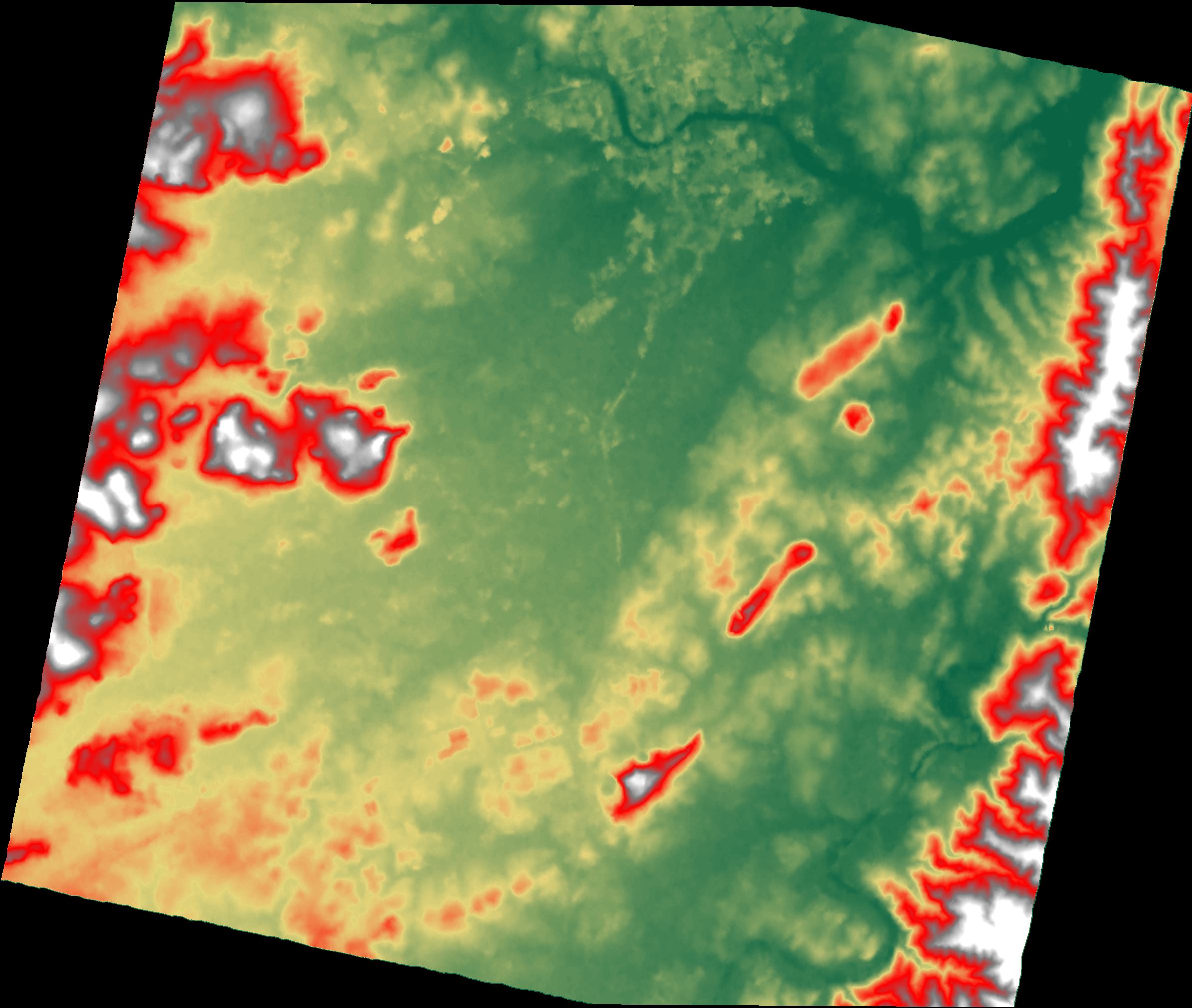
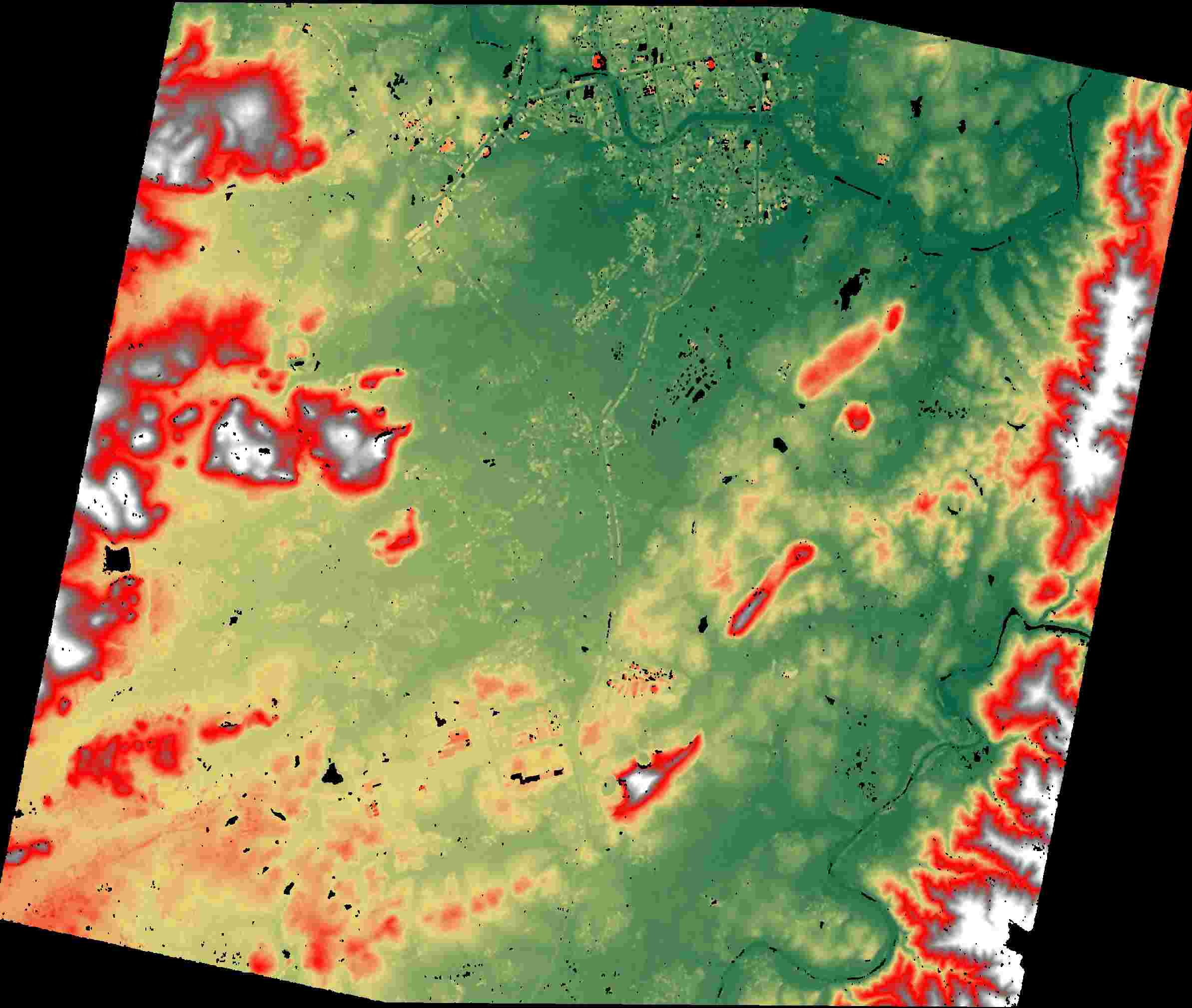
image2

(a) GT

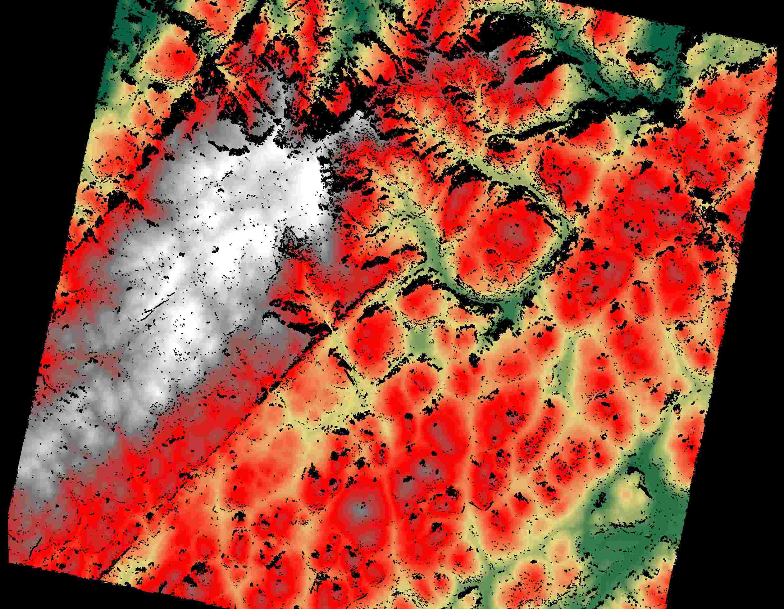
(b) S2P

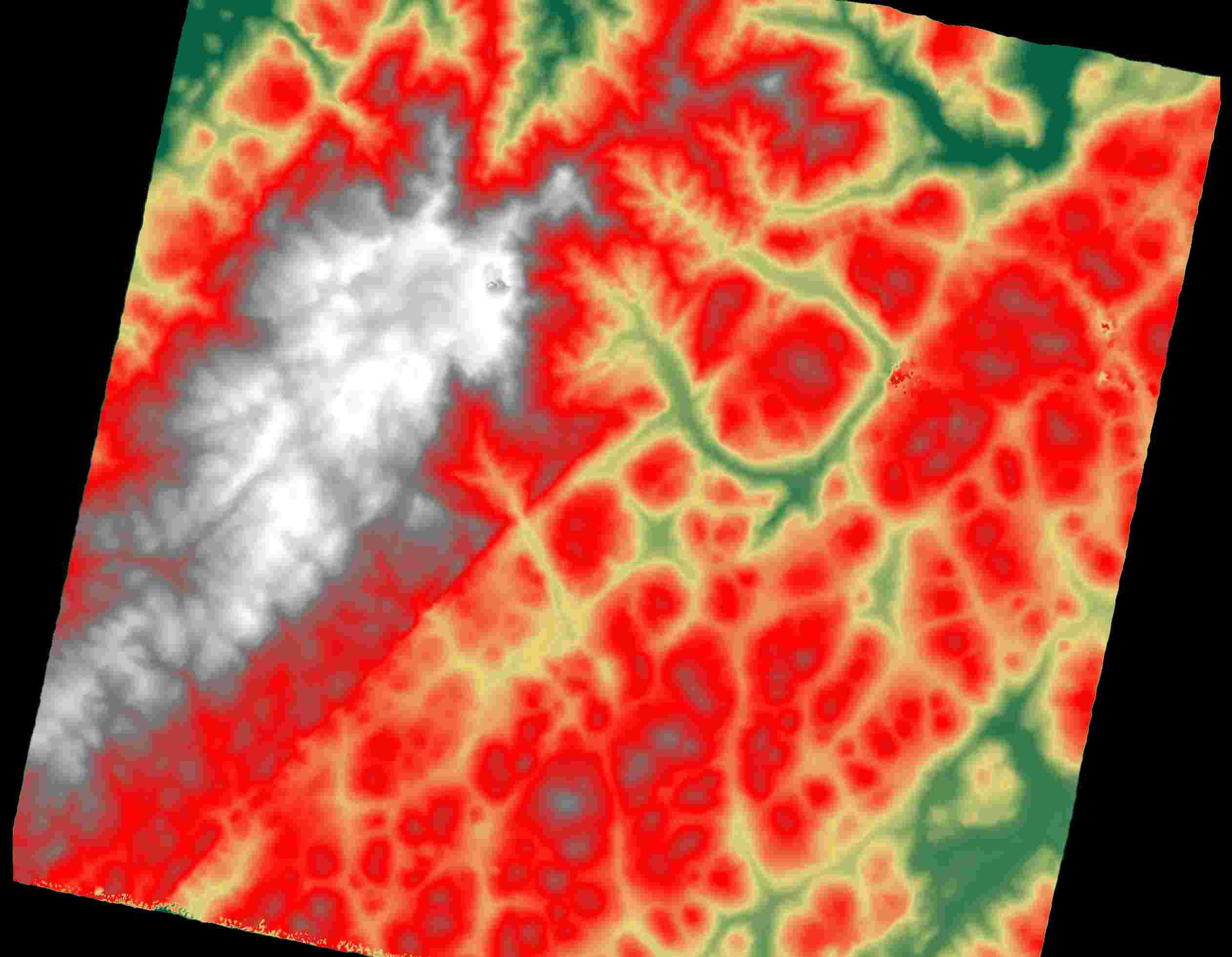
(c) LPS

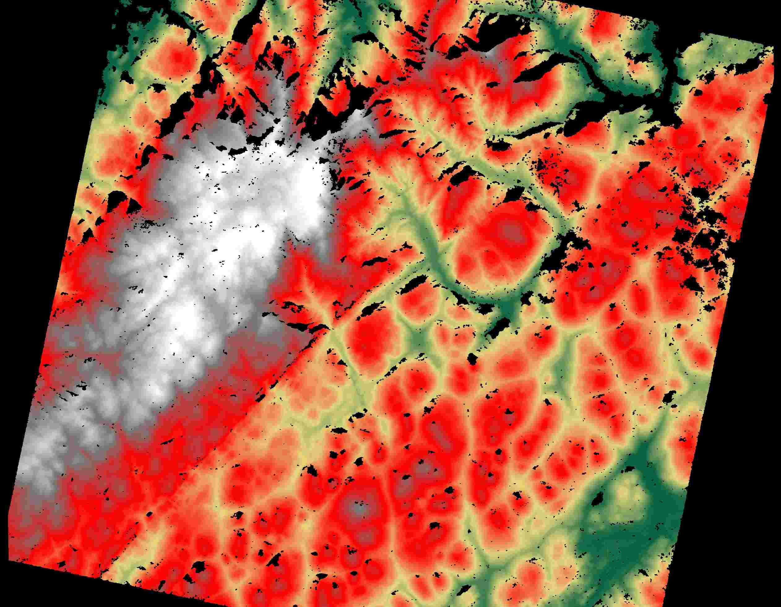
(d) AC

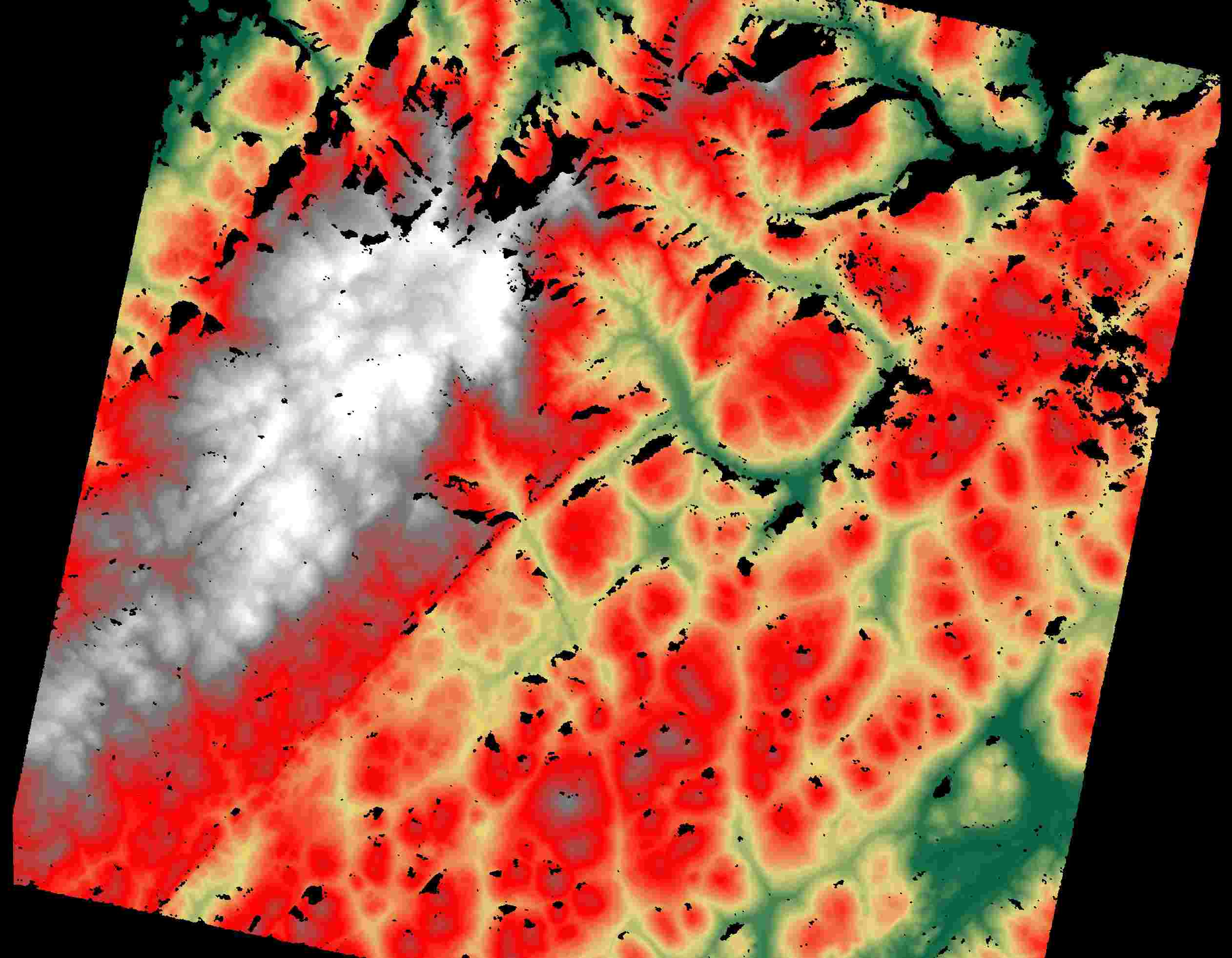
(e) Ours

image1

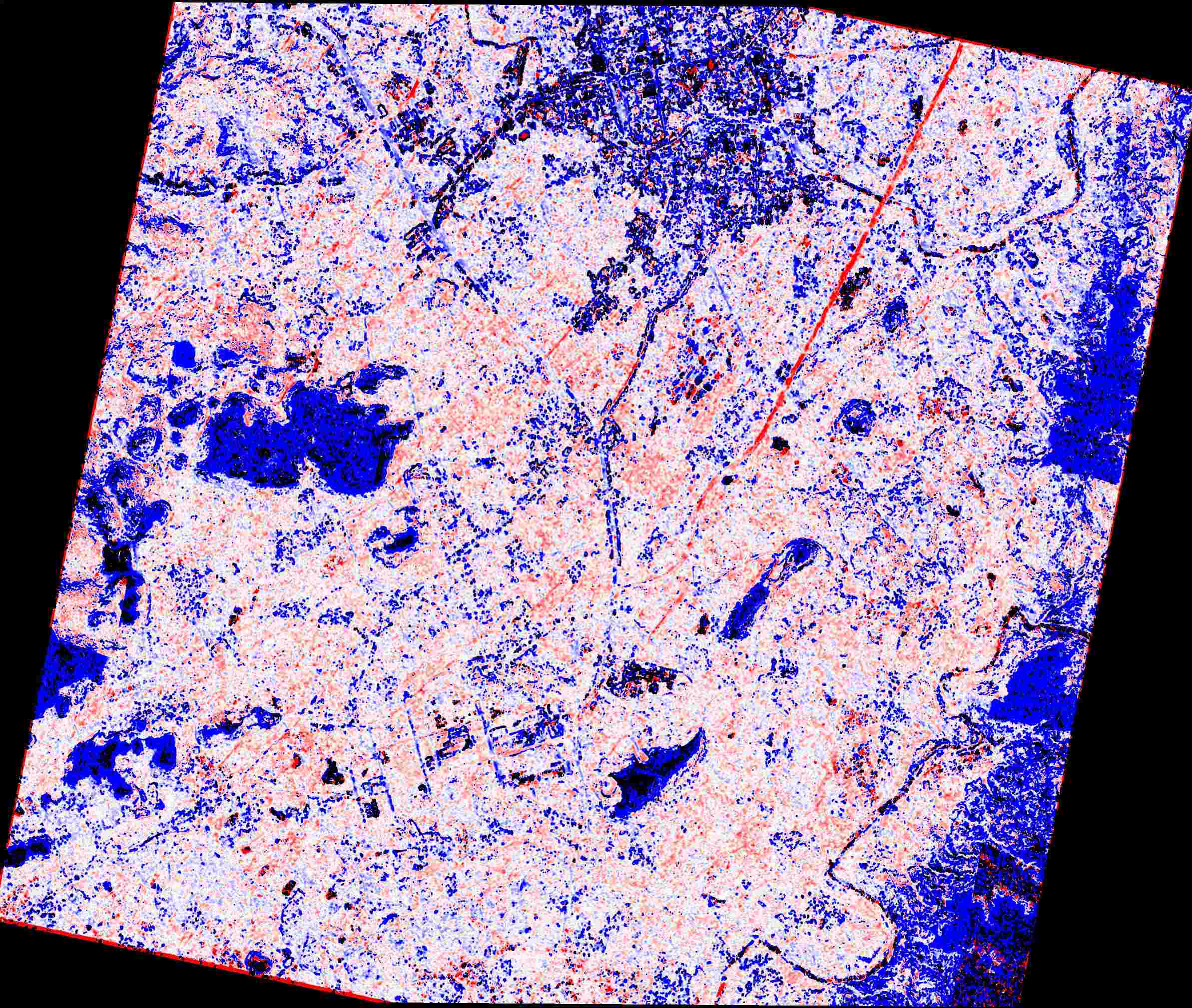
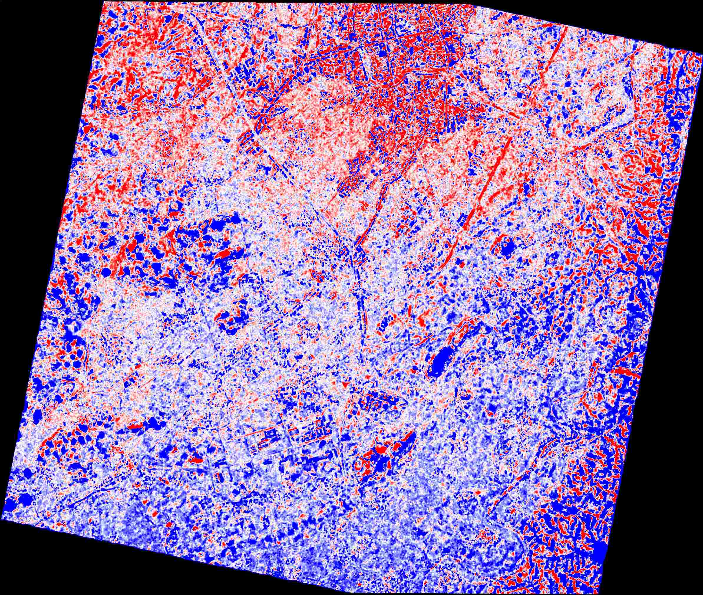
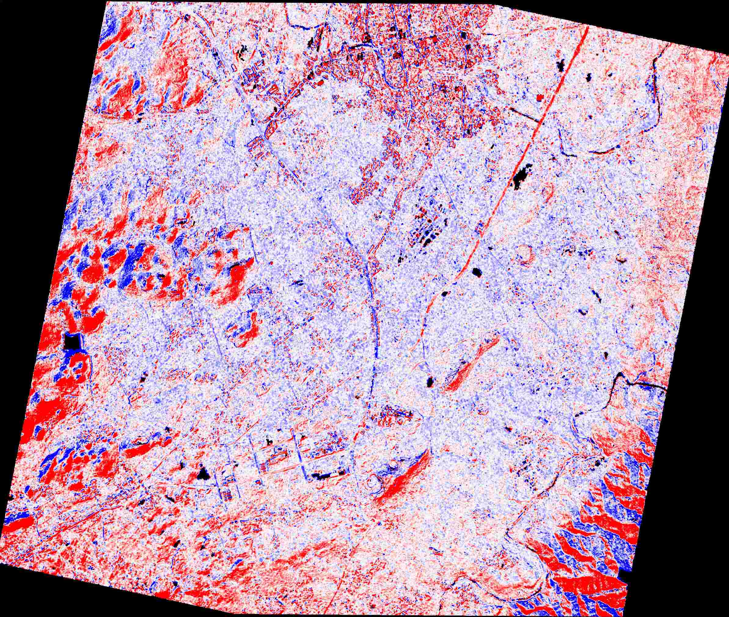
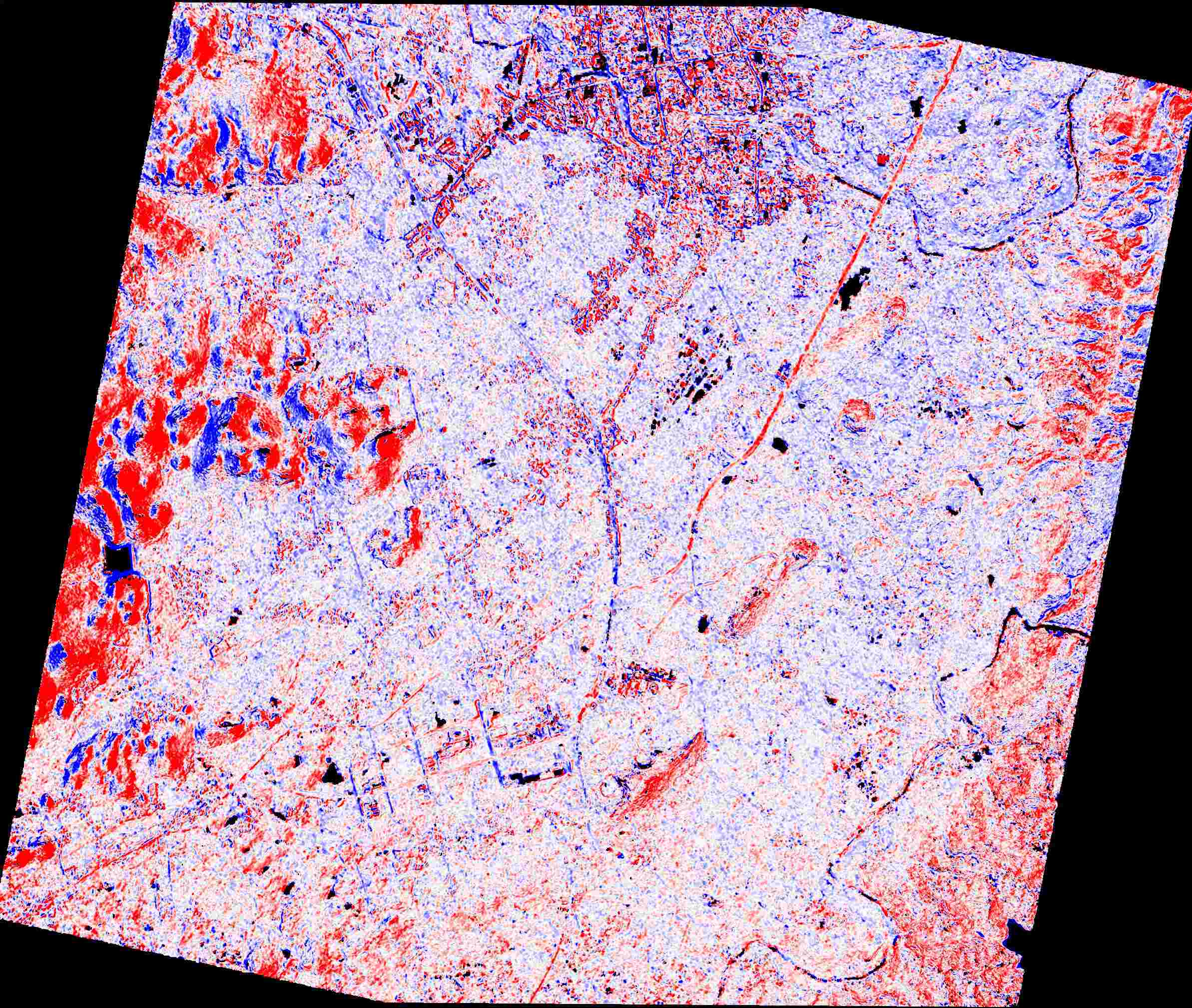
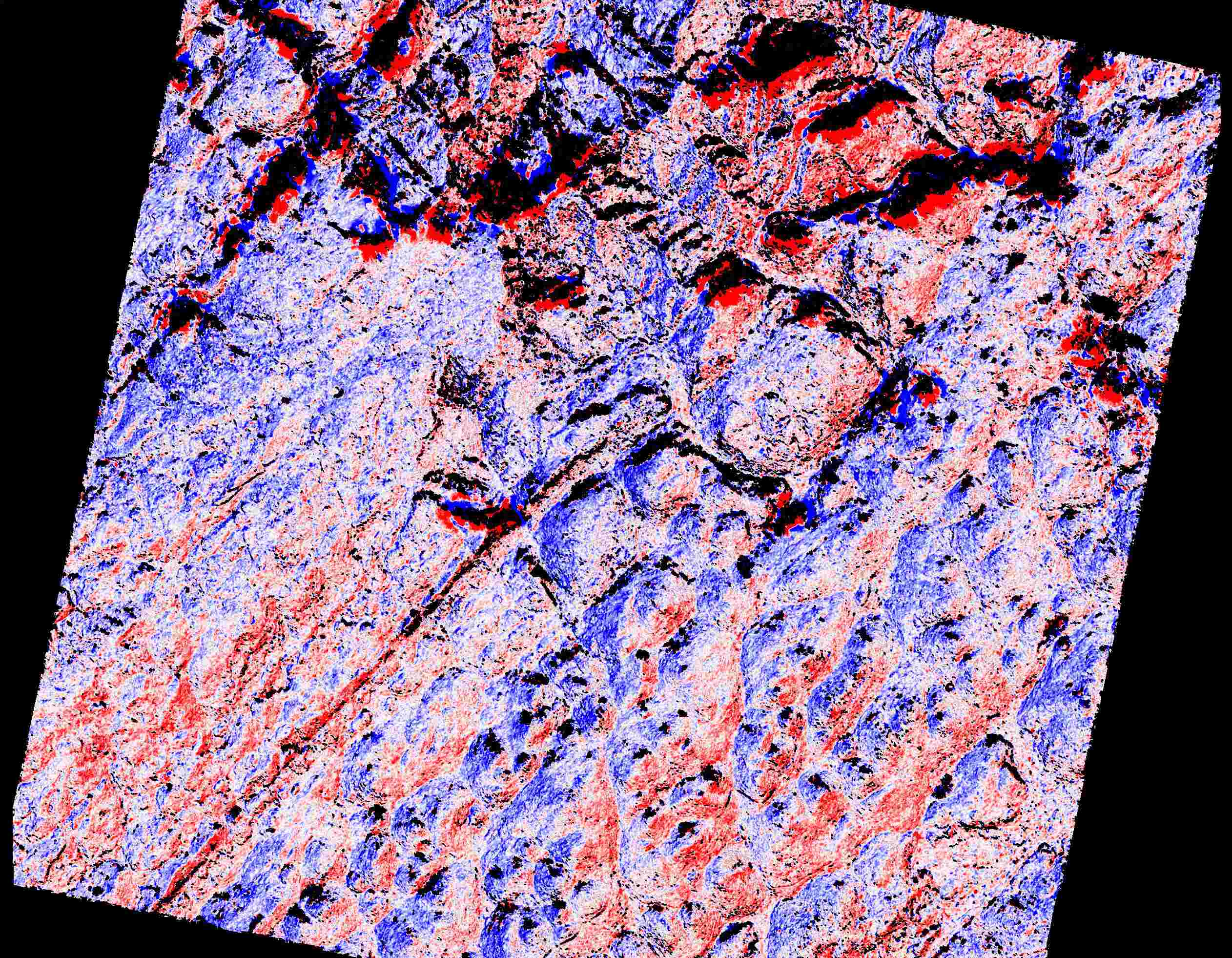
image2

(f) S2P

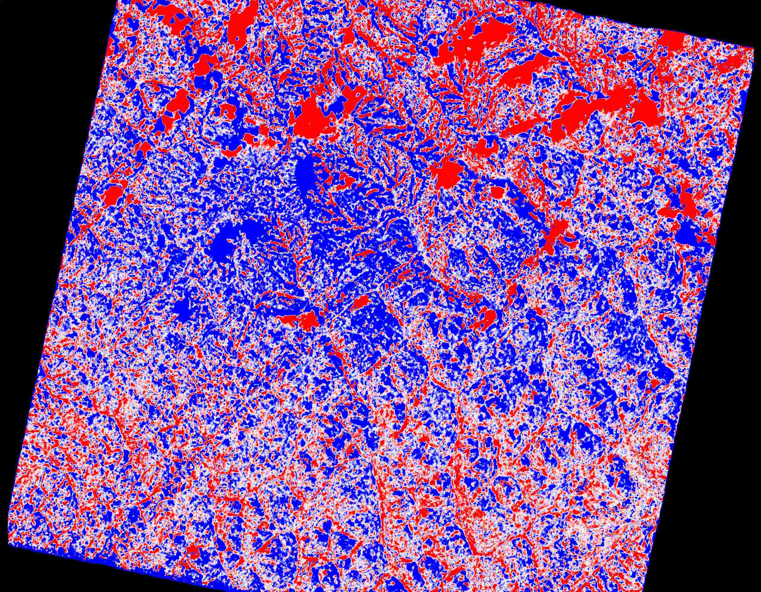
(g) LPS

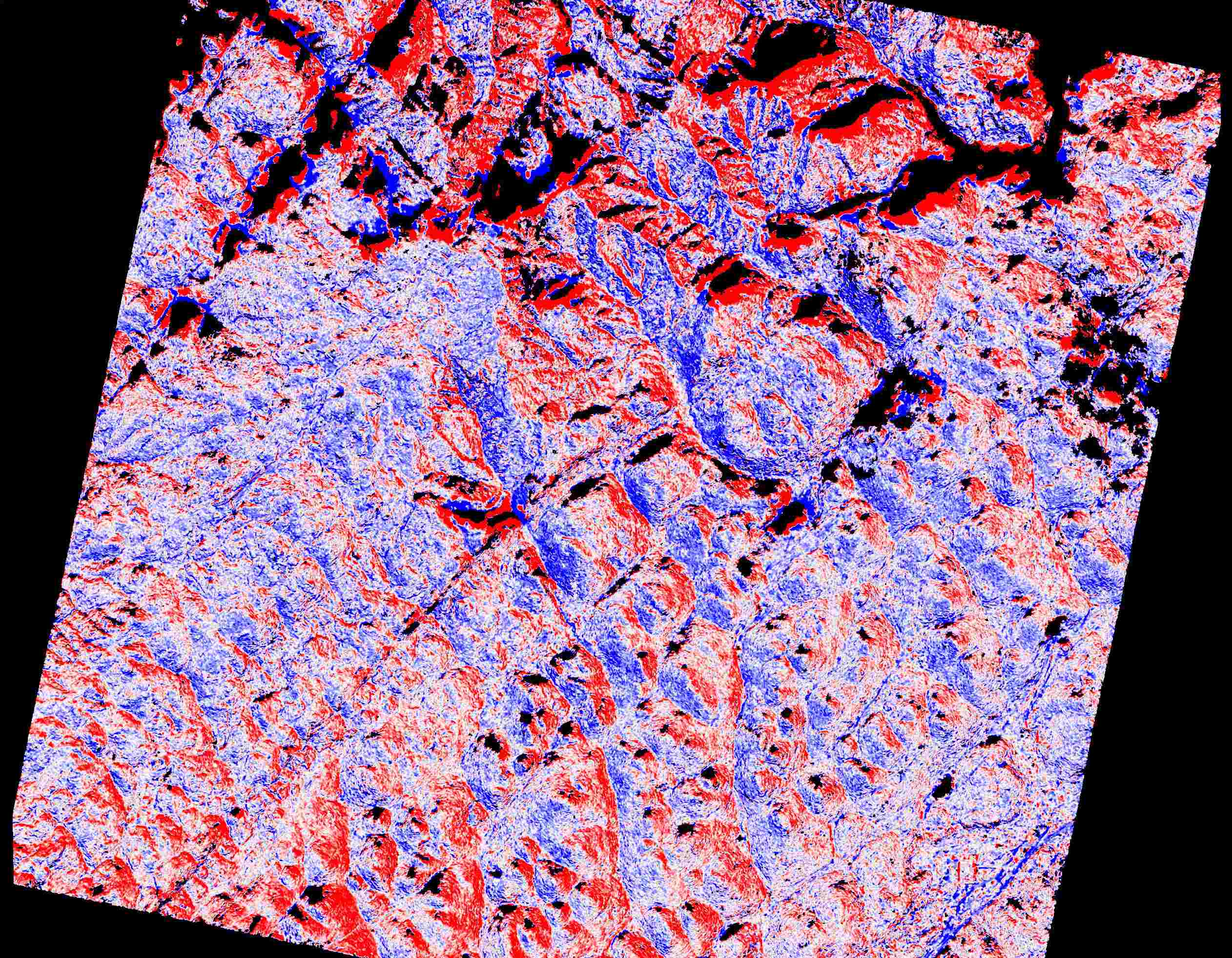
(h) AC

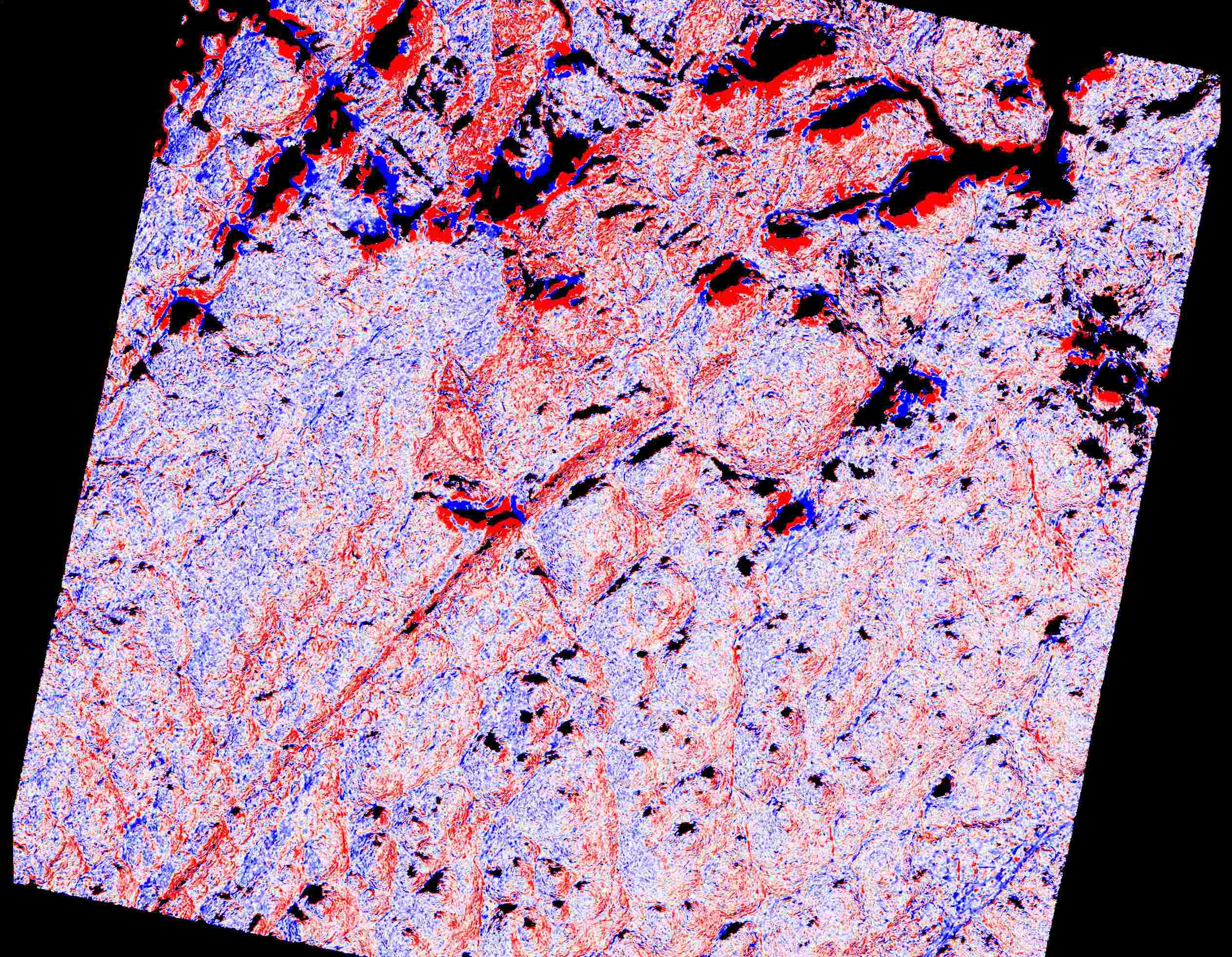
(i) Ours

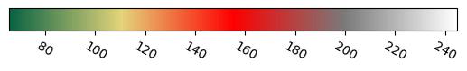
(j) Image1 bar

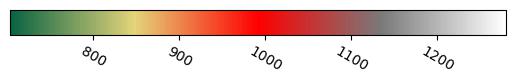
(k) Image2 bar

(l) Error bar

Figure 4: Examples of DSMs and error plots for different solutions of the WHU-TLC test set. The color bar is expressed in units of meters.

4.2.2 Results for the DFC2019 dataset

We conducted a comparative study using four prevalent sites in the DFC2019 dataset. For each of the four sites, we performed simple artificial masking of water bodies based on pixel values. Each site includes various satellite images obtained from different dates, and S2P and our pipeline could perform multi-view 3D reconstruction. LPS generated a DSM for every two images, and we selected the one with the highest accuracy, as listed in Table 2. In the DFC2019 dataset, the accuracy of our method and the Adapted COLMAP were essentially the same, but the completeness of our method was significantly higher than that of the other methods.

Table 2: Quantitative results of DSM reconstruction quality on the WoildView3 image data. (Bold works best).

Site	Methods	ME (m)$\downarrow$	RMSE (m)$\downarrow$	Comp1 (%)$\uparrow$	Time (min.)$\downarrow$
JAX_004	S2P	0.293	2.822	60.318	40.192
	LPS	0.858	3.136	53.763	12.440
	AC	0.381	3.453	63.737	6.740
	Ours	0.386	3.326	63.770	7.317
JAX_068	S2P	0.202	2.467	69.430	11.281
	LPS	0.993	4.358	50.193	10.143
	AC	0.239	3.883	72.849	13.279
	Ours	0.260	3.753	72.450	14.406
JAX_214	S2P	0.234	3.630	54.459	39.185
	LPS	1.463	8.629	42.943	14.305
	AC	0.326	4.868	65.957	17.072
	Ours	0.353	4.893	66.014	18.287
JAX_260	S2P	0.577	9.452	36.045	30.047
	LPS	1.600	12.831	38.122	13.297
	AC	0.592	3.812	59.938	12.551
	Ours	0.599	3.865	60.451	13.390

Table 2 shows that S2P achieved a higher accuracy. However, compared to our method, the S2P reconstruction failed in more areas, and the completeness at a threshold of 1 m was worse, causing a maximum drop of approximately 40% and a minimum drop of approximately 4%. By combining the DSM reconstruction results shown in Fig. 5 and the error maps presented in Fig. 6, our method performed exceptionally well for vegetation, roads, and the edges of buildings. Fig. 6 displays the error maps of the DSM against the true DSM. Our method exhibited superior accuracy in estimating the heights of buildings and roads, but its accuracy was relatively low for vegetation and building shadows. The DSMs reconstructed by LPS exhibited a lower accuracy overall, possibly because the LPS method’s 3D reconstruction of multi-date VHR imagery without GCPs is poor.

JAX_004

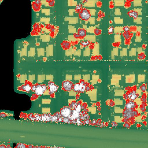
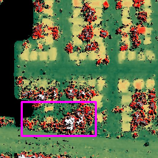
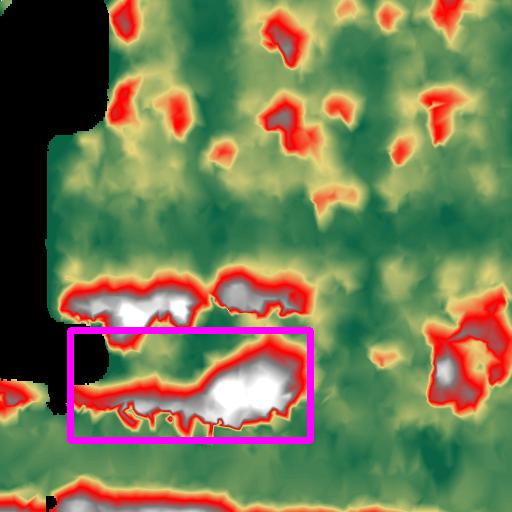
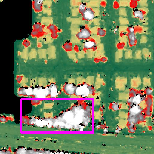
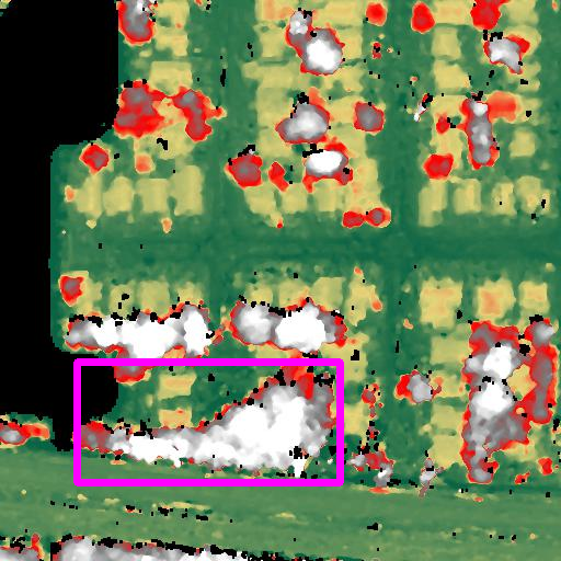
JAX_068

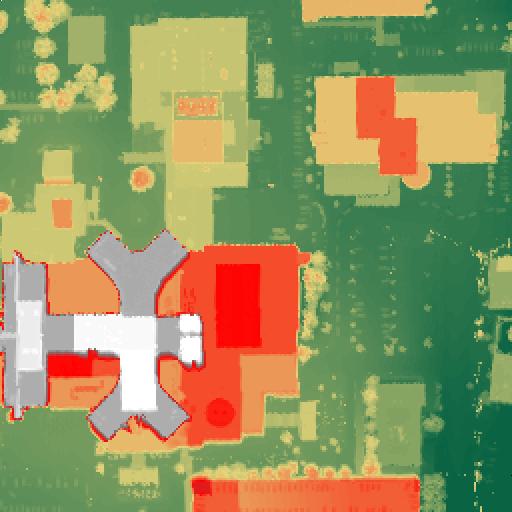
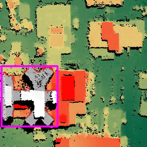
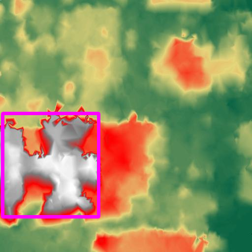
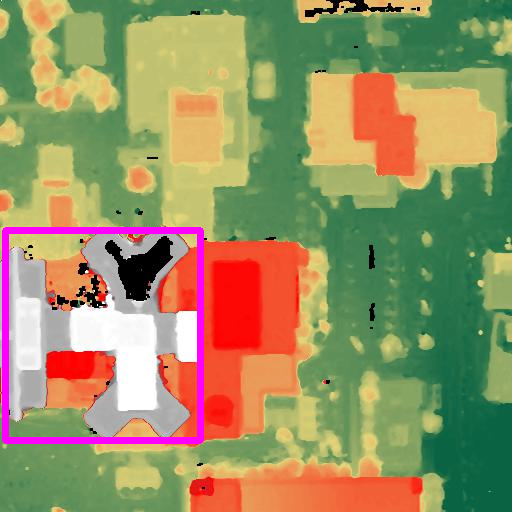
JAX_214

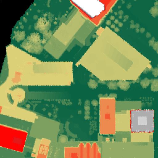
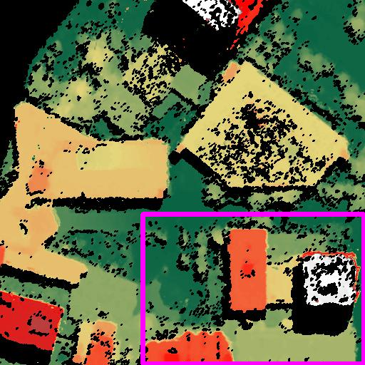
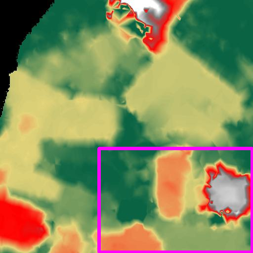
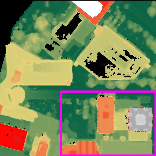
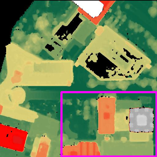
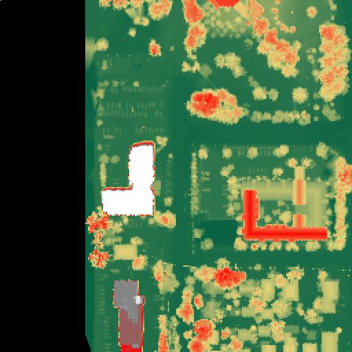
JAX_260

(a) GT

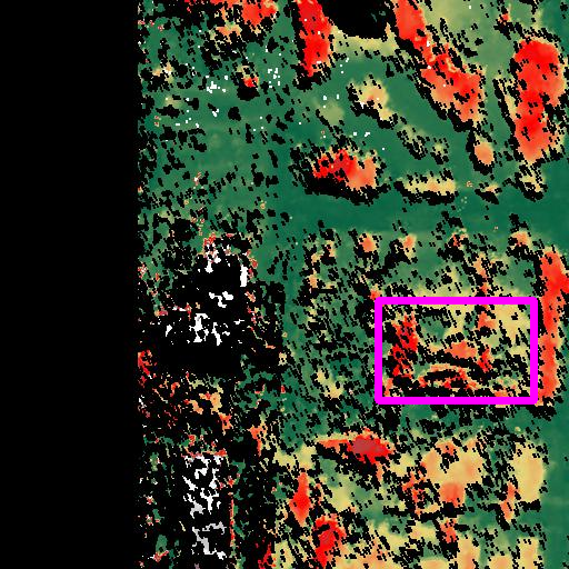
(b) S2P

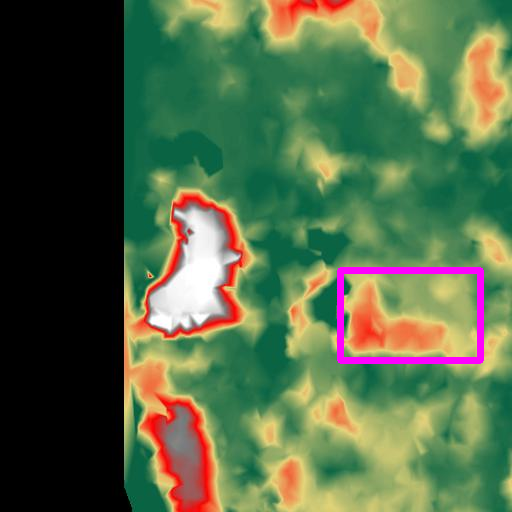
(c) LPS

(d) AC

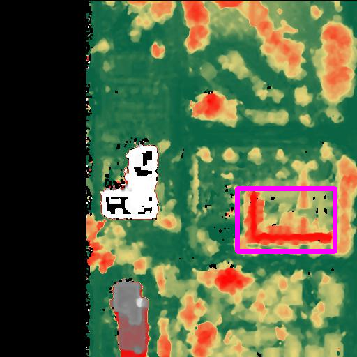
(e) Ours

Figure 5: DSM results for the DFC dataset. The color bars of JAX_004, JAX_068, JAX_214, and JAX_260 are represented by (f), (g), (h), and (i), respectively. The color bar is expressed in units of meters.

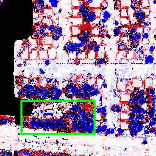
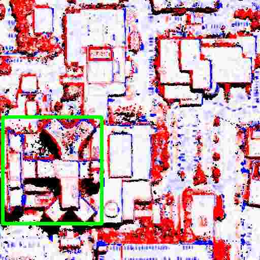
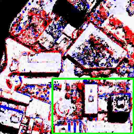
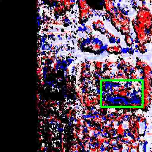
(a) S2P

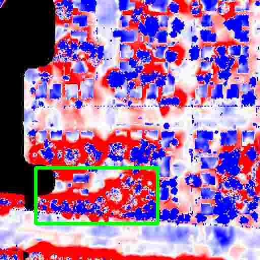
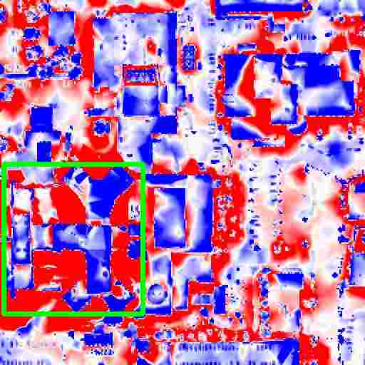
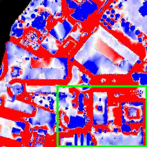
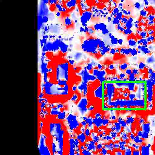
(b) LPS

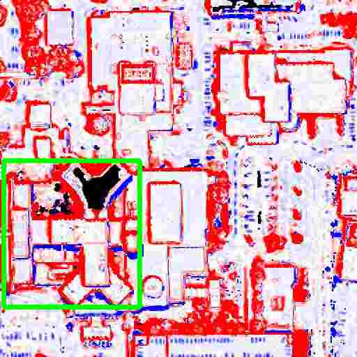
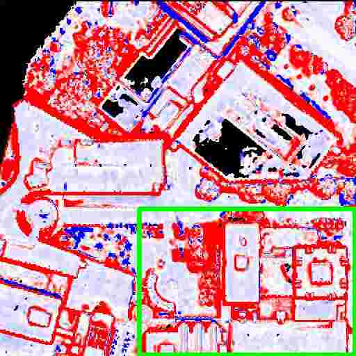
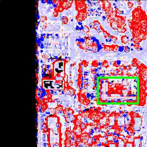
(c) AC

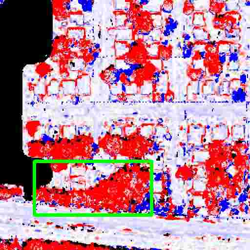
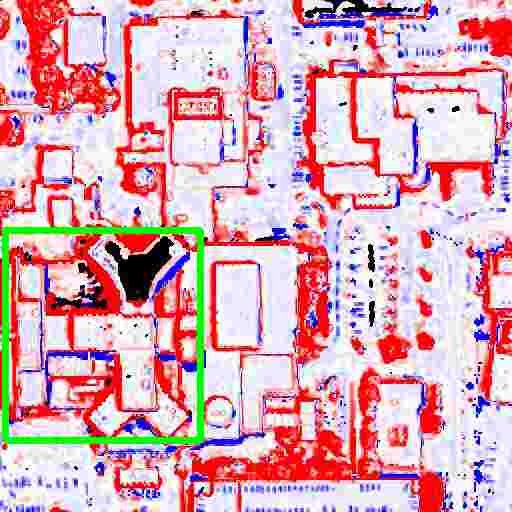
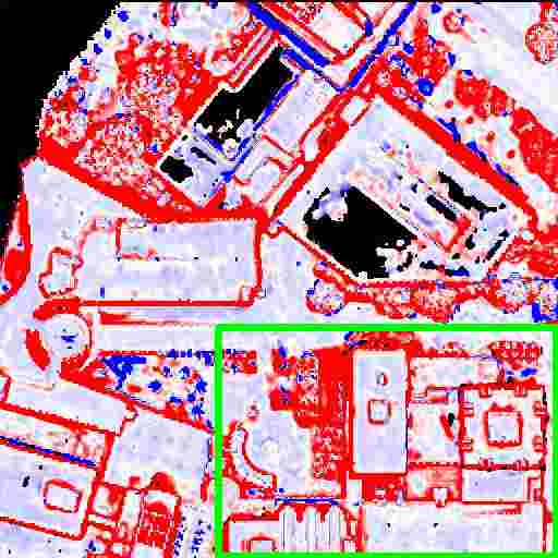
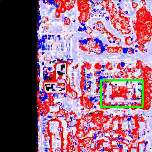
(d) Ours

Figure 6: Error maps of on the DFC dataset. The color bar is expressed in units of meters.

4.2.3 Results for the ISPRS-ZY3 dataset

Because the data for the Sainte-Maxime region in the ISPRS ZY3 satellite imagery contained GCPs, we assessed the absolute positioning accuracy of these data. We first calculated the altitude accuracy of the stereo positioning of the checkpoints for the RPC model’s image space compensation scheme, as shown in Table 3. We then examined the corresponding altitudes of the GCPs in the reconstructed DSM and calculated the median, RMSE, and maximum of the altitude errors. For this large-scale satellite image, the Adapted COLMAP generated NA. Table 3 demonstrates that the addition of the image refinement model dramatically improved the precision of our method, which exhibited an accuracy comparable to S2P. In addition, our method attained optimality regarding both the median and maximum errors. The final results of our REPM pipeline are presented in Fig. 7 (water is filtered out in the pipeline).

Table 3: Absolute accuracy comparison of reconstruction outcomes for Sainte-Maxime, France in the ISPRS-ZY3 image data is undertaken employing GCP. (Bolded is the best, underlined is the second best.)

Methods	ME (m)$\downarrow$	RMSE (m)$\downarrow$	Max (m)$\downarrow$
RPC model localization	2.668	4.053	8.508
S2P	3.464	3.679	6.308
LPS	6.779	7.629	13.276
REPM	12.122	12.353	18.960
REPM+Ref.	3.442	3.812	5.862

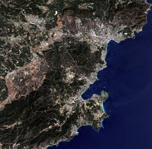
(a) The true color image ISPRS (2018)

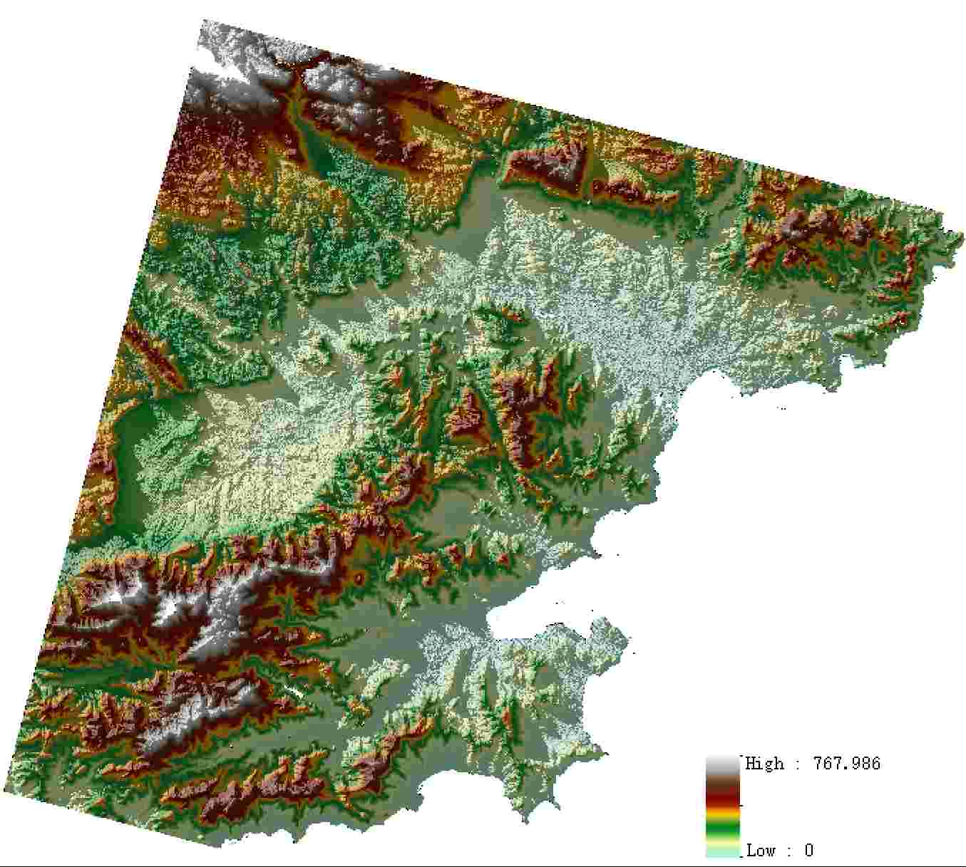
(b) DSM

Figure 7: Results produced by our REPM pipeline for the Sainte-Maxime dataset: (a) true color image and (b) DSM product.

4.2.4 Results for the GF7 dataset

In the experiments with the Gaofen7 (GF7) image of the Zhengzhou region, we used the reference image as a benchmark to calculate the accuracy and completeness of the reconstructed DSM. The quantitative results are presented in Table 4, and Fig. 8 displays the DSM reconstruction results and error maps for partial areas.

Table 4: Quantitative results of DSM reconstruction quality on the GF7 image data. (Bold works best)

Methods	ME (m)$\downarrow$	MAE (m)$\downarrow$	RMSE (m)$\downarrow$	Comp2 (%)$\uparrow$
S2P	0.725	0.398	3.492	74.810
LPS	2.912	5.630	12.037	32.401
REPM	1.280	0.973	3.303	74.917
REPM+Ref.	0.939	0.622	2.804	77.367

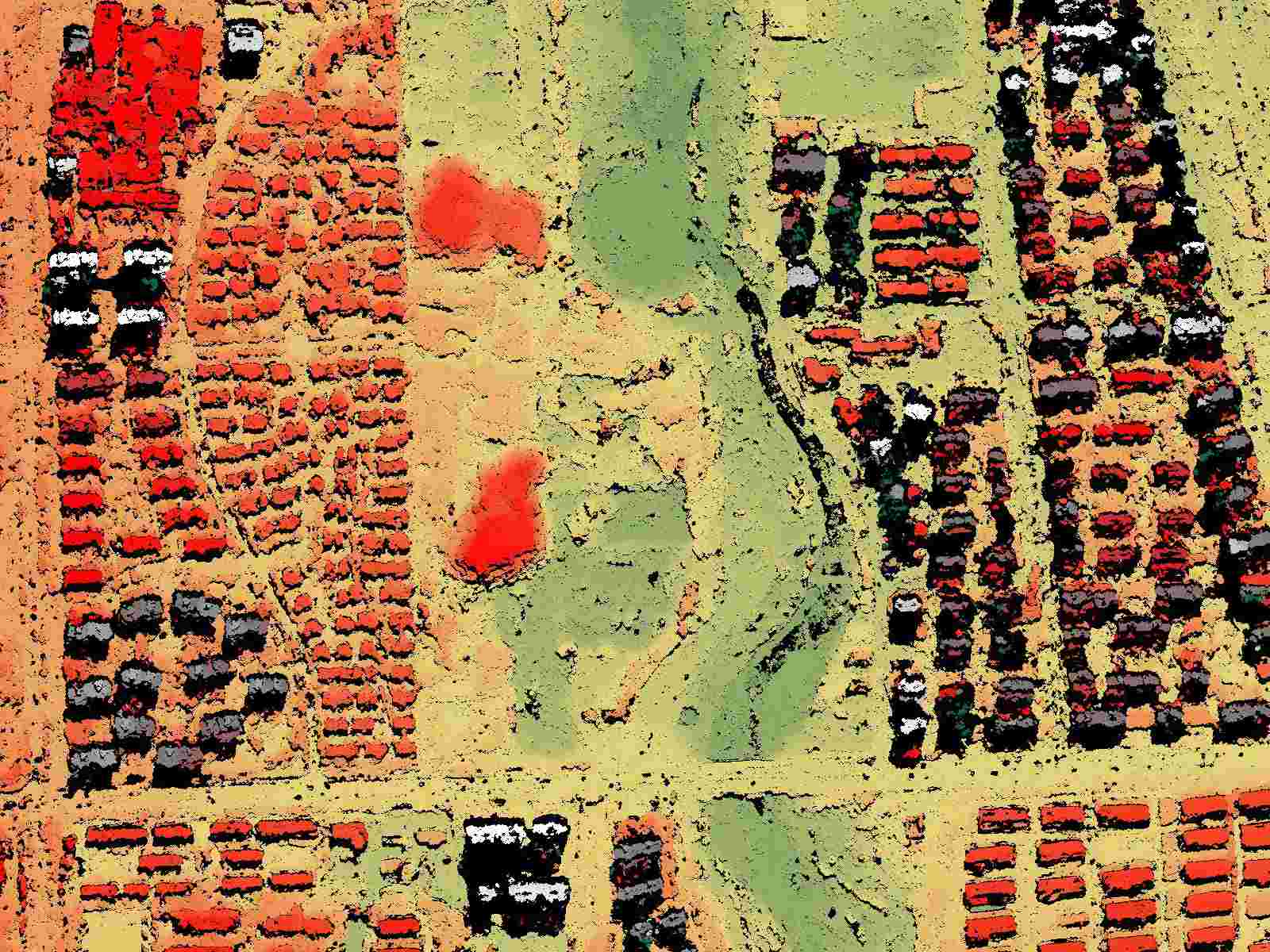
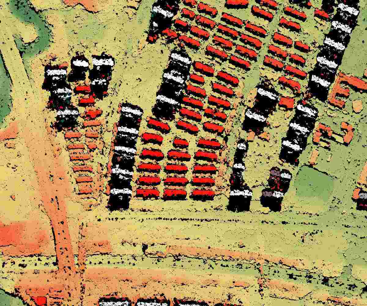
(a) Reference

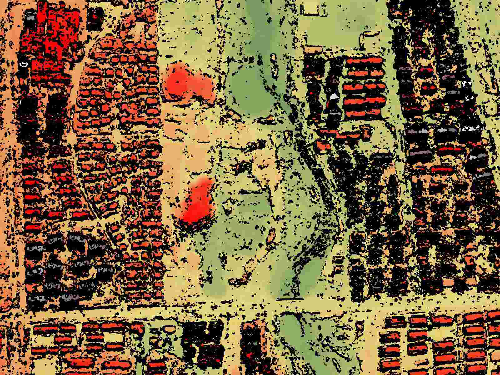
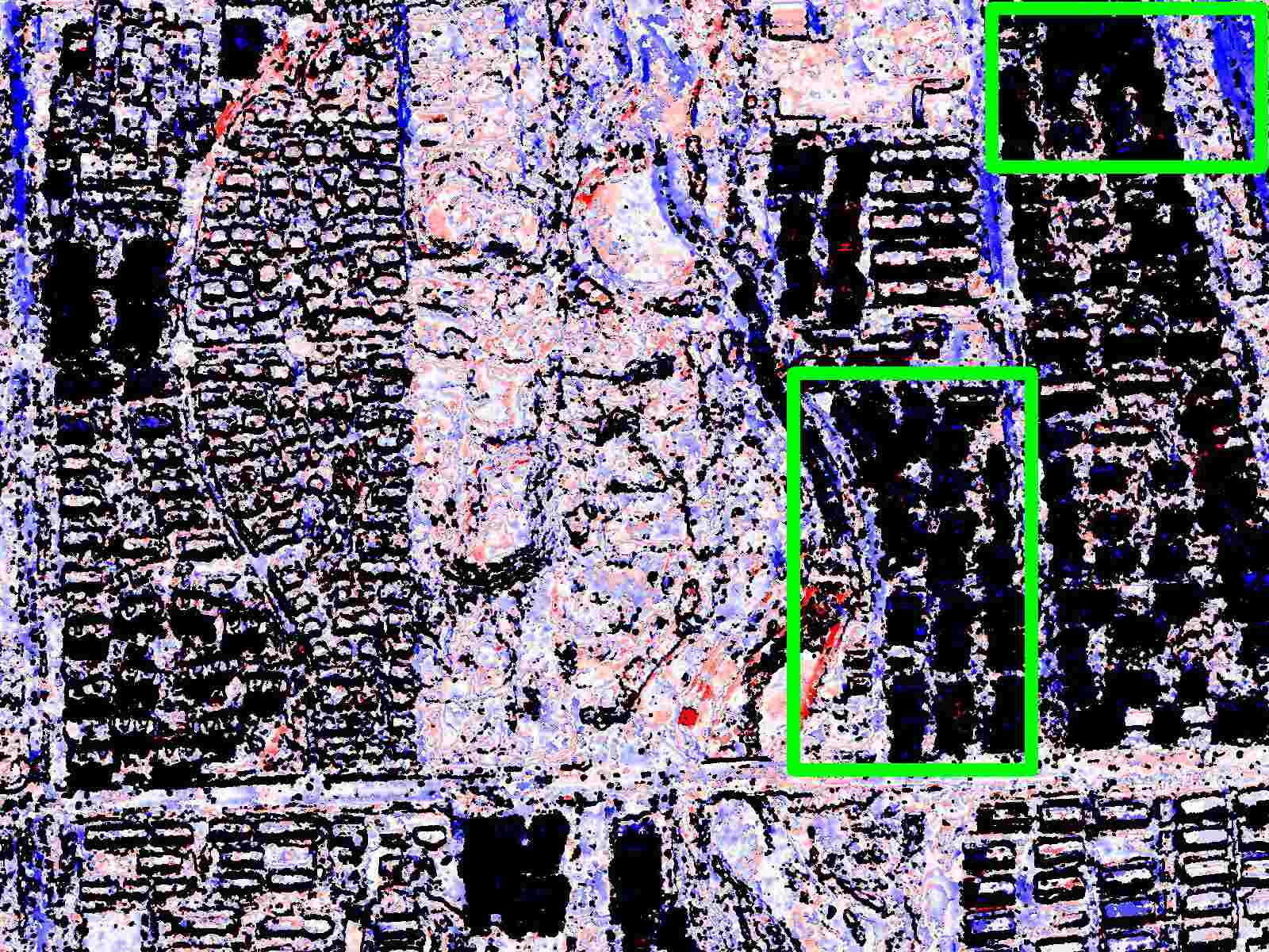
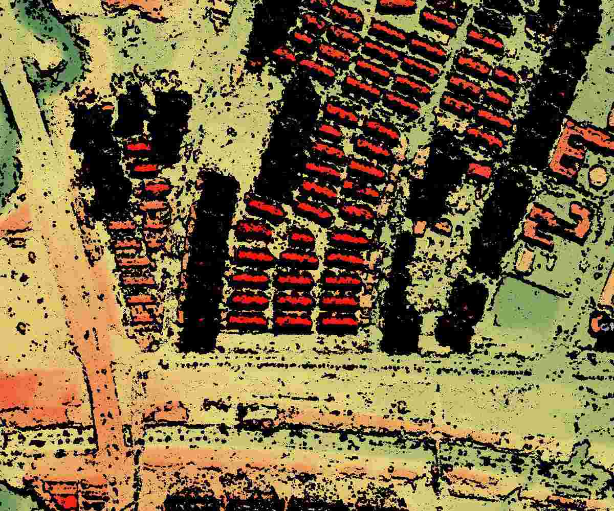
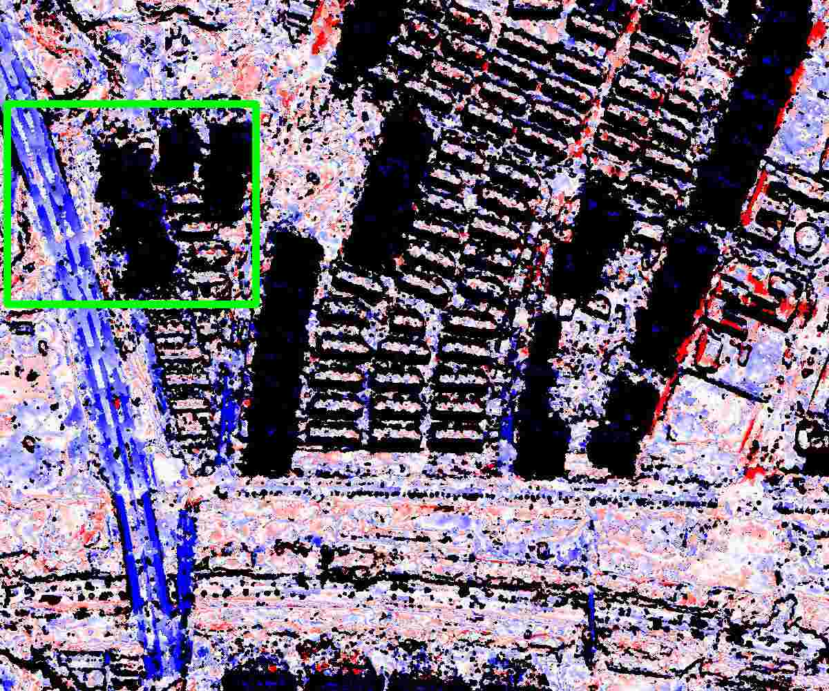
(b) S2P

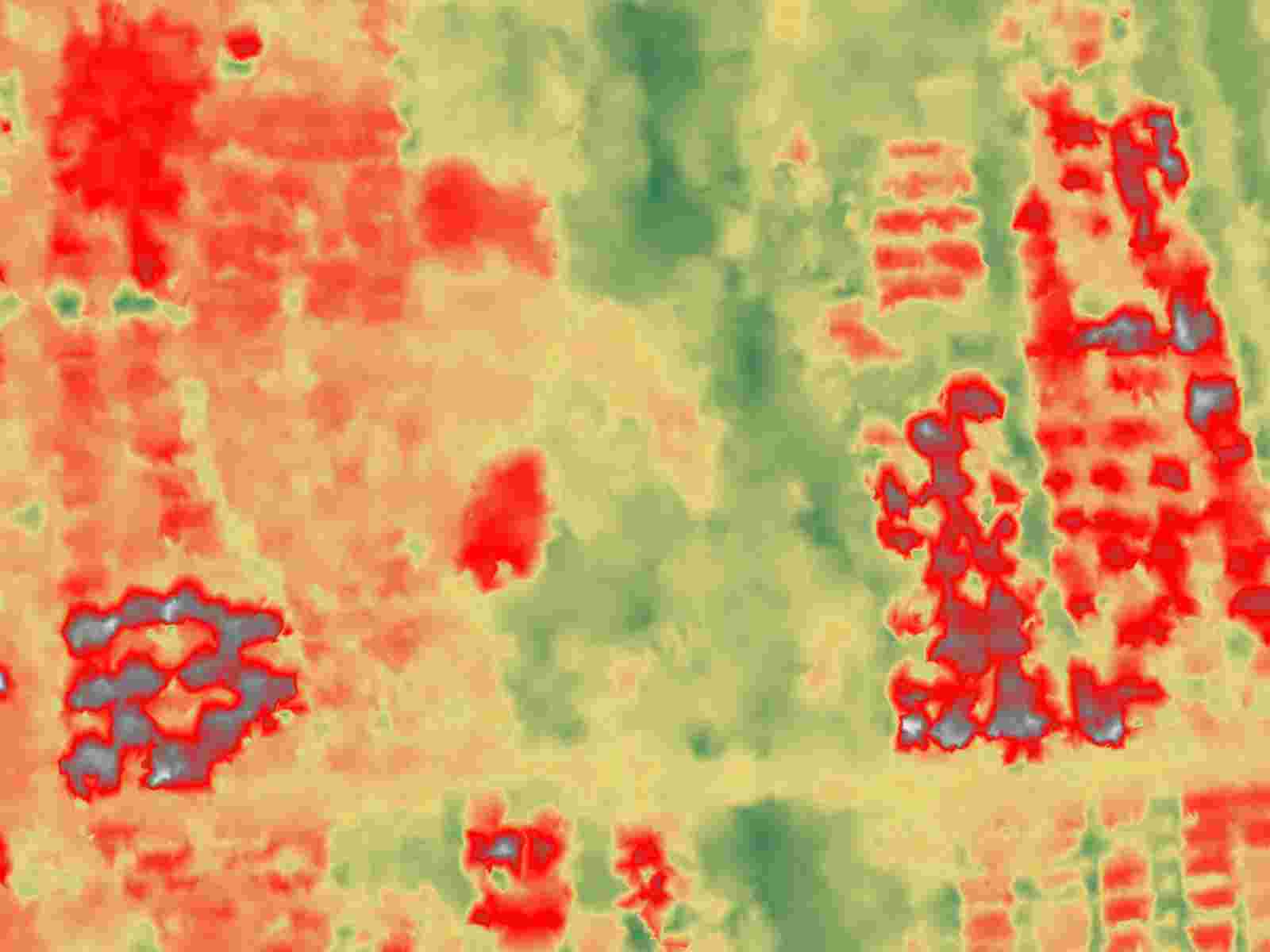
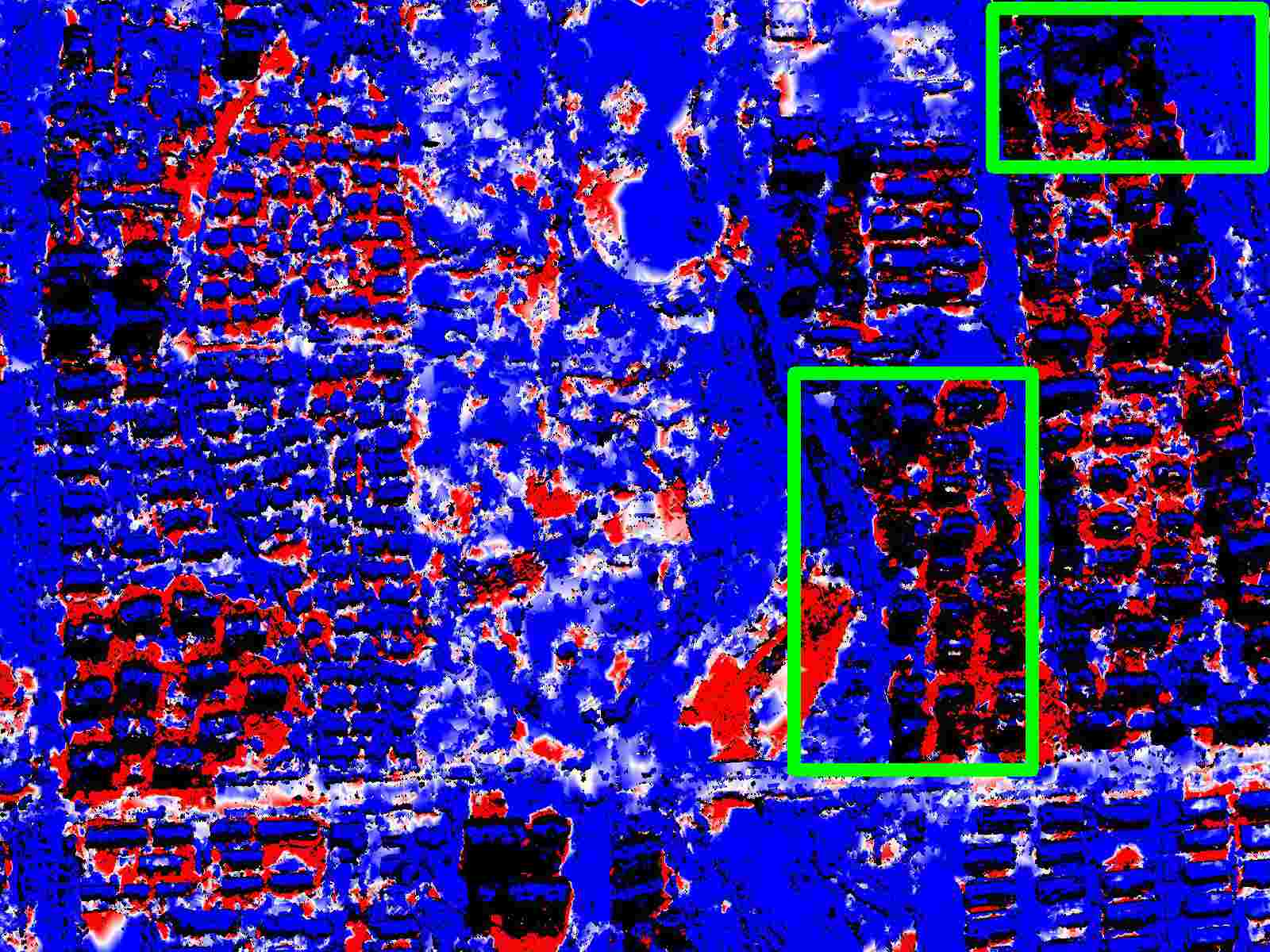
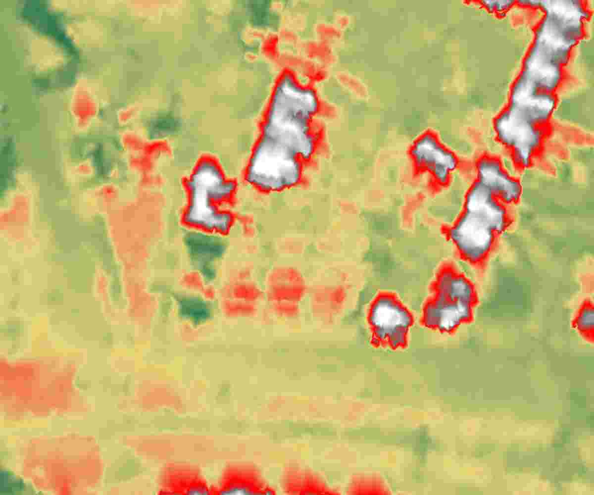
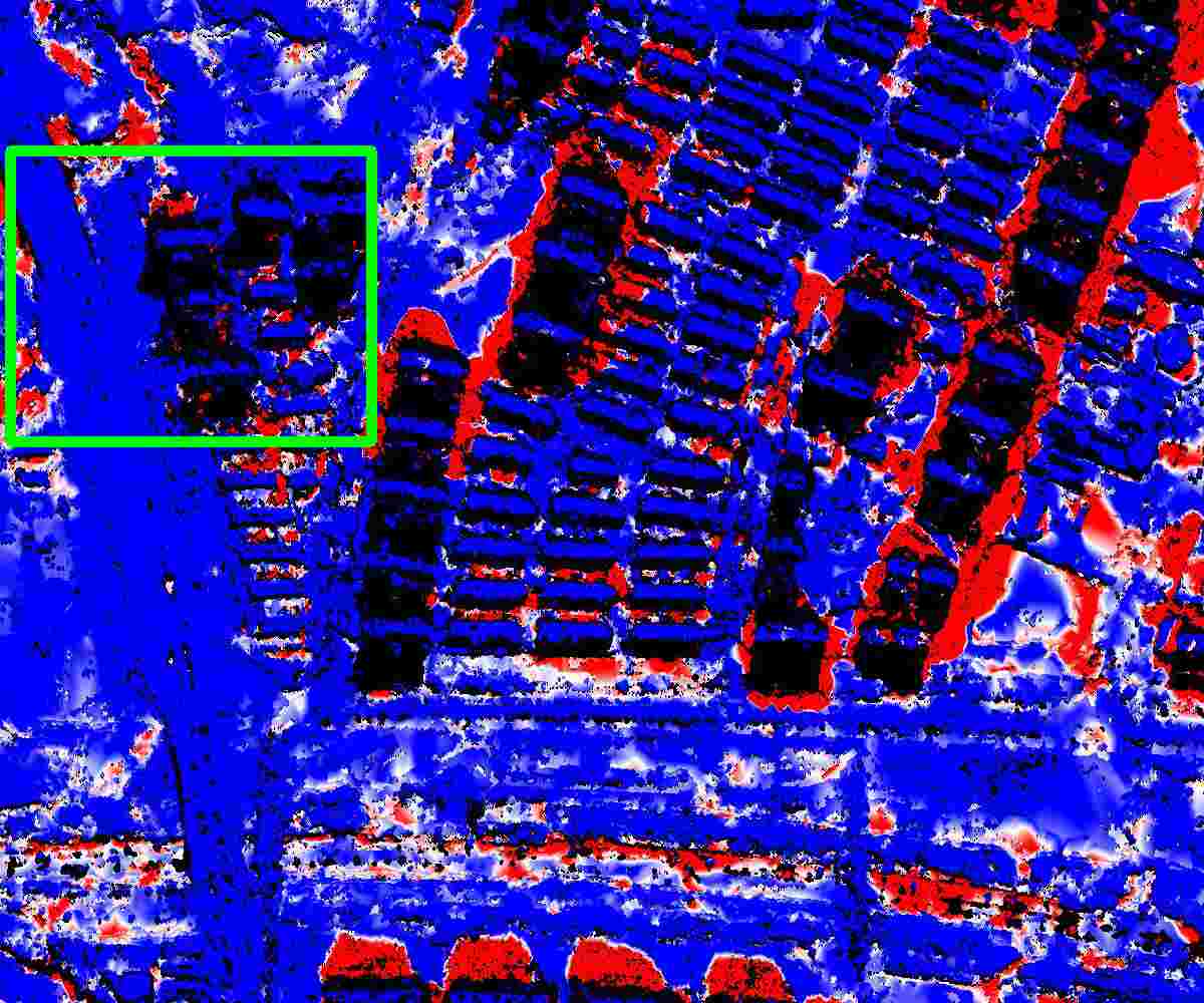
(c) LPS

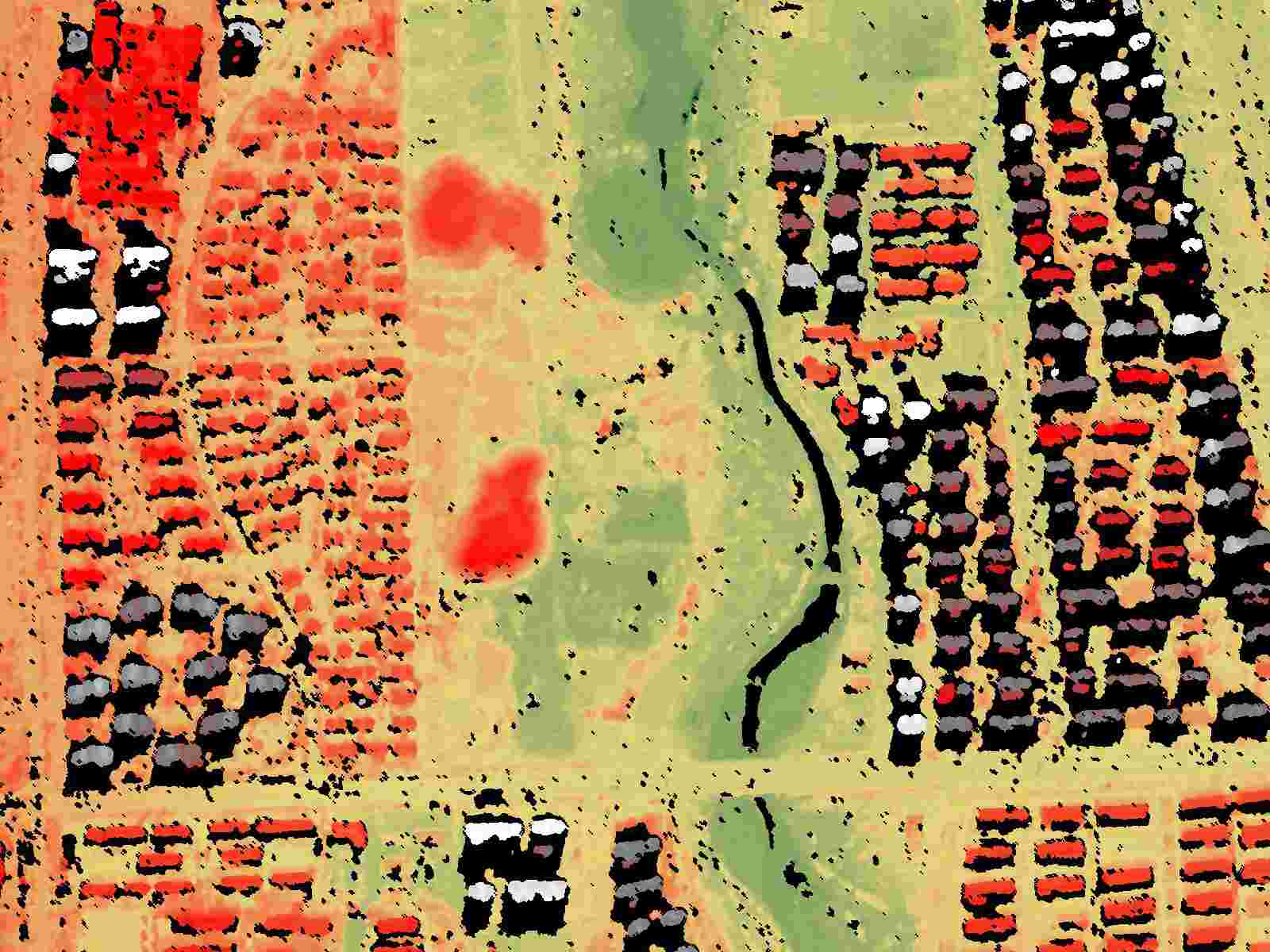
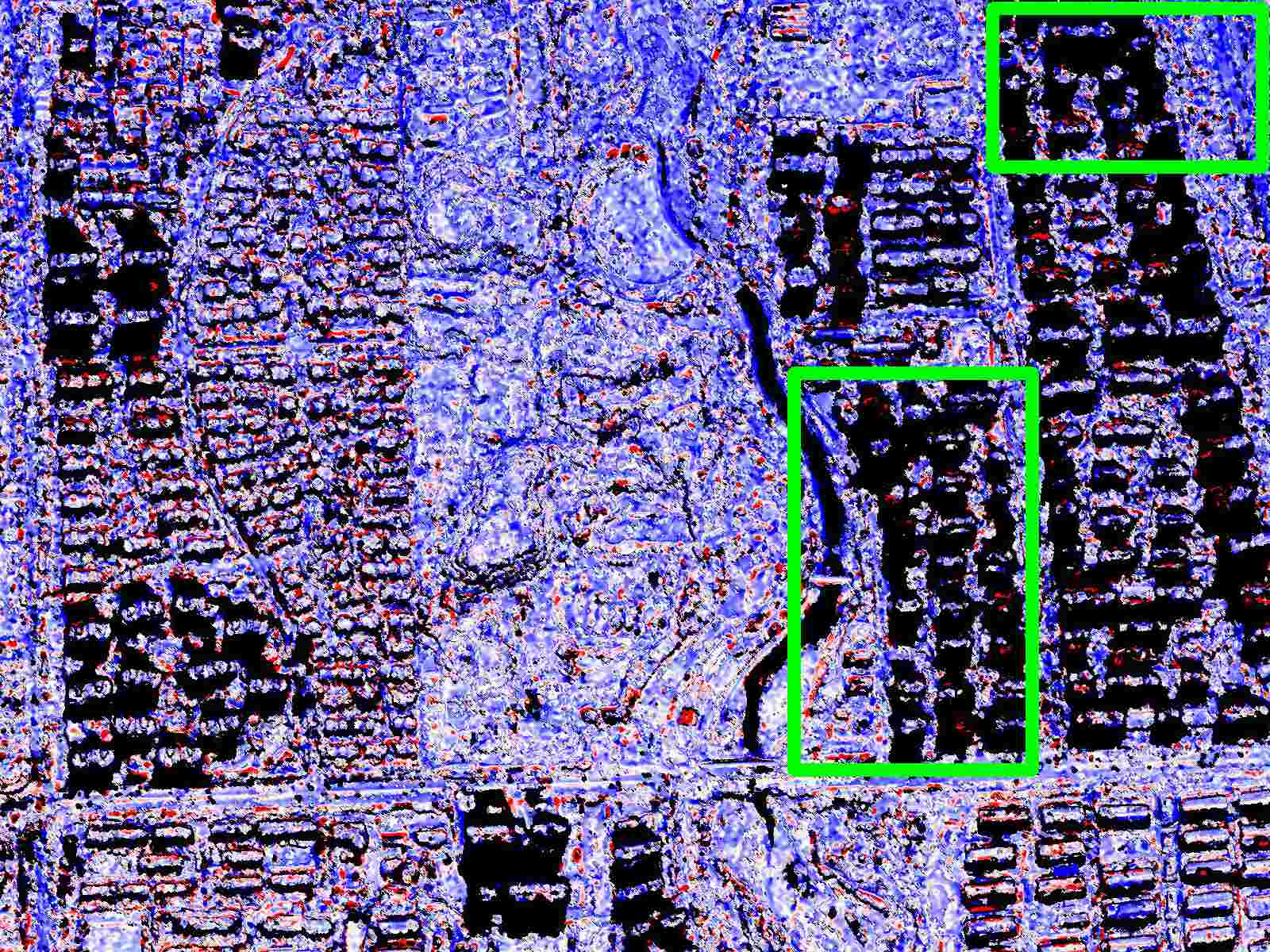
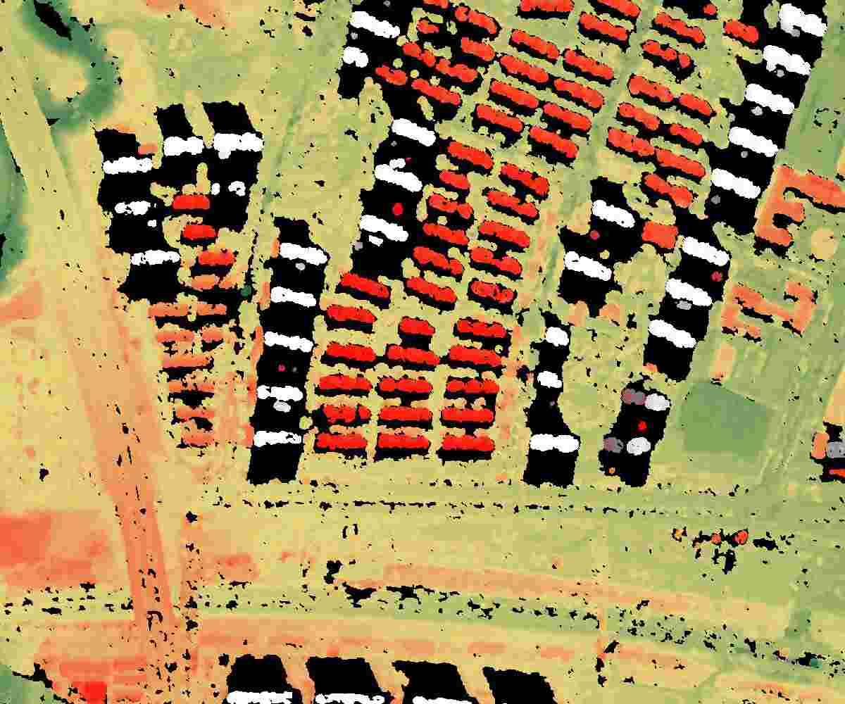
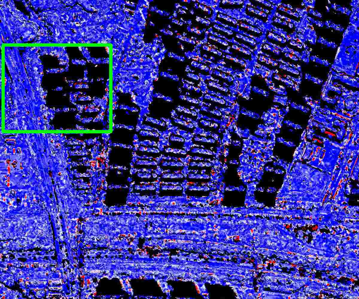
(d) REPM

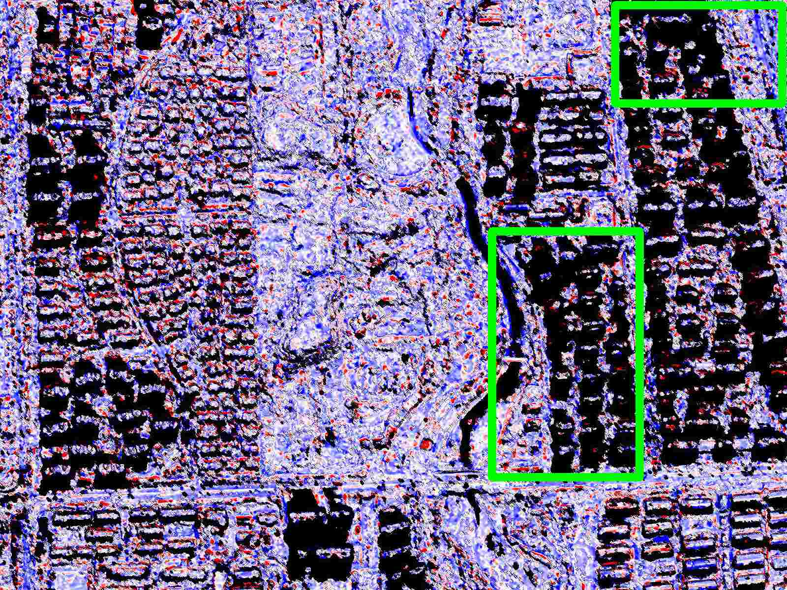
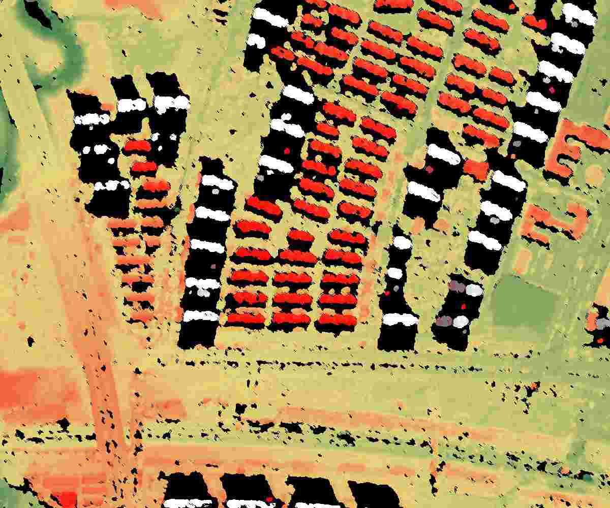
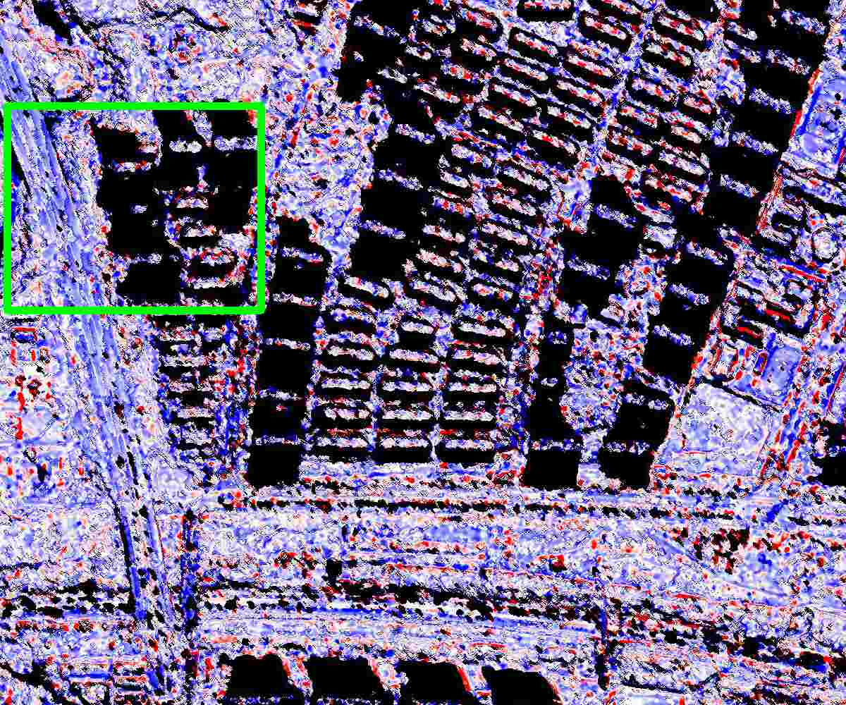
(e) REPM+Cor.

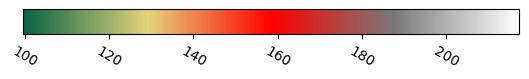
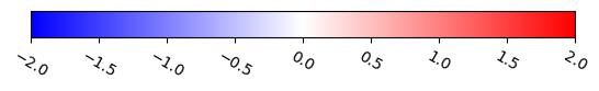
Figure 8: Partial DSM results and error plots for the GF7 image data. The color bar is expressed in units of meters.

As shown in Table 4, our method achieved the highest reconstruction accuracy and completeness, and the incorporation of the image refinement model significantly boosted the accuracy and completeness with a threshold of 2 m. Fig. 8 shows the DSM reconstruction results for local areas. For high-resolution images of urban areas, we mainly compared the reconstruction results of buildings and roads. Our method was optimal in terms of the completeness and accuracy for buildings. In contrast, S2P was unsuccessful in reconstructing tall buildings (white buildings). Furthermore, LPS lost detailed building information, and the overall height estimation accuracy was poor.

5 Discussion

5.1 Summary of the reconstruction results

In the DSM reconstruction experiments on the four datasets, we can draw the following conclusions.

(1) The proposed REPM pipeline significantly outperforms all the other methods, including both the software and open-source solutions, in terms of the two accuracy metrics of RMSE and Comp. When comparing the reconstructed DSMs and error maps, it can be observed that the pipeline proposed in this paper has yielded the highest accuracy and completeness.

(2) The incorporation of a polynomial image refinement model has proven to further enhance the accuracy and completeness of the DSM reconstruction. Additionally, it is worth noting that for imaging on a large-scale, the DSM reconstruction accuracy and completeness is significantly improved.

5.2 Influence of the equivalent pinhole model

According to the equivalent error formula presented in Section 3.2, the factors that affect the equivalent error are directly proportional to the size of the image and the difference in terrain altitude. In the experiment, we primarily explored the effect of the image size on the equivalent error. We defined the equivalent error $L_{E}$ as the distance between the position of pixel $p$ computed using the RPC parameter and the position of pixel $p^{\prime}$ computed using the KRT parameter for the same object point, as displayed in Eq. (13). We used Eq. (8) to calculate the RMSE accuracy of the equivalent error.

$$RMSE=\sqrt{(Samp\ RMSE)^{2}+(Line\ RMSE)^{2}}$$ (12)

$$L_{E}=\sqrt{(x_{p}-x_{p^{\prime}})^{2}+(y_{p}-y_{p^{\prime}})^{2}}$$ (13)

For satellite CCD images within a specific dataset, the error is directly proportional to the image size. For the same image size, as the image resolution increases, the equivalent error increases. The impact of image resolution on the equivalent error can be viewed as follows: as the image resolution increases, the terrain area corresponding to the same image size decreases, which indirectly affects the altitude difference and decreases it. According to Eq. (13), the equivalent error is proportional to the altitude difference. In summary, the image resolution indirectly affects the equivalent error for the same image size; as the image resolution increases, the equivalent error increases.

Additionally, Fig. 9 displays the distribution of pixel-level equivalent errors on the image, providing a visual representation of the impact of image size on the equivalent error. Evidently, the equivalent error decreases as the image size decreases, eventually resulting in subpixel precision.

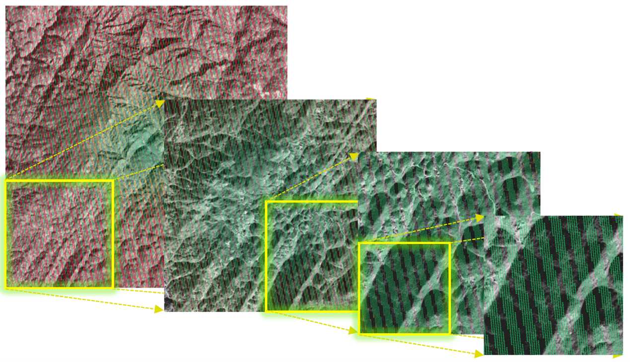
Figure 9: Visualizations of the distribution of the equivalent error on the image and the relationship between the equivalent error and the image size. The color bar is expressed units of pixels.

Next, we examine the impact of the image size on the reconstructed DSMs in the WHU-TLC dataset, as presented in Table 5. The reduction in image size improved the ME accuracy and DSM completeness, but decreased the RMSE accuracy. Nevertheless, based on the results shown in Fig. 10, the altitude error in the error map display decreased as the image size decreased. In the second group of images, which had substantial differences in altitude, the reconstruction precision declined significantly when the image size was reduced from 1024 pixel to 512 pixel. This underscores the importance of selecting an optimal image size. We conclude that reducing the image size leads to an exponential increase in the number of images required, which creates a more complex stereo-matching view-selection problem in the pipeline reconstruction process, resulting in a decrease in the reconstruction accuracy.

Table 5: Influence of image size on reconstruction accuracy for same region on WHU-TLC test set.

Crop Size	ME (m)$\downarrow$	RMSE (m)$\downarrow$	Comp2.5 (%)$\uparrow$	Comp5 (%) $\uparrow$
$512$	0.919	4.291	79.864	91.374
$1024$	0.925	3.940	79.547	91.204
$2048$	0.991	3.843	78.827	90.979
$5120$	1.146	3.334	73.926	88.244

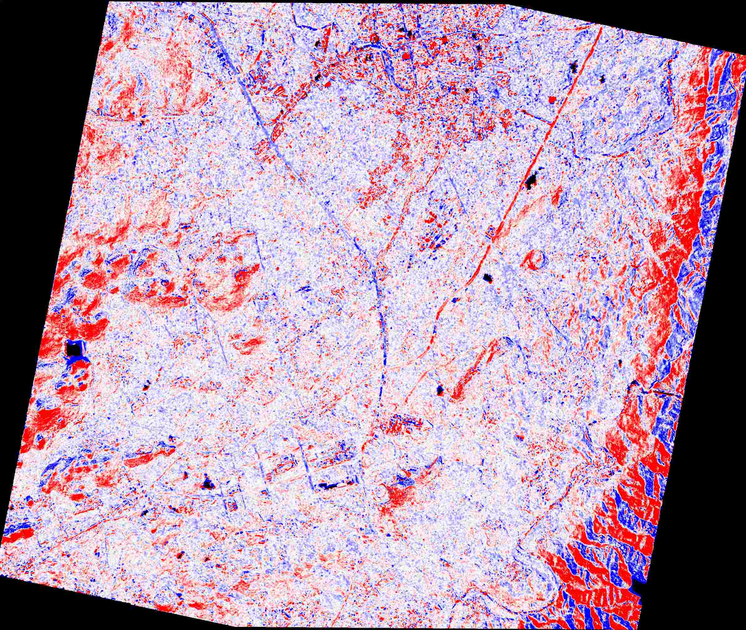
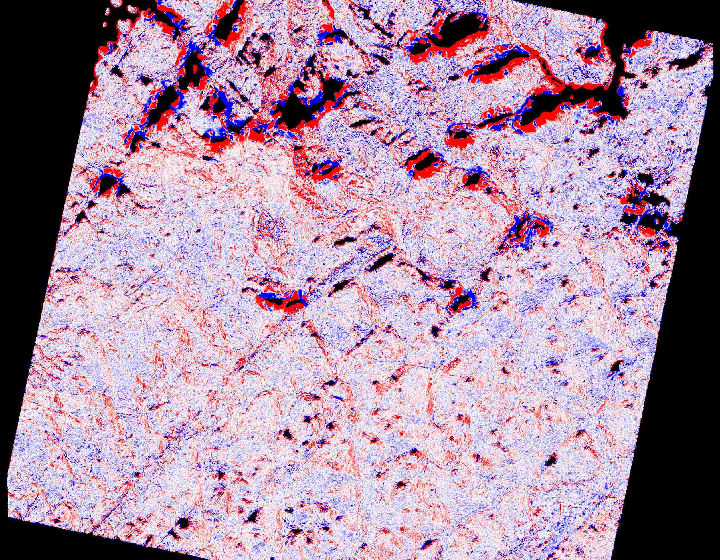
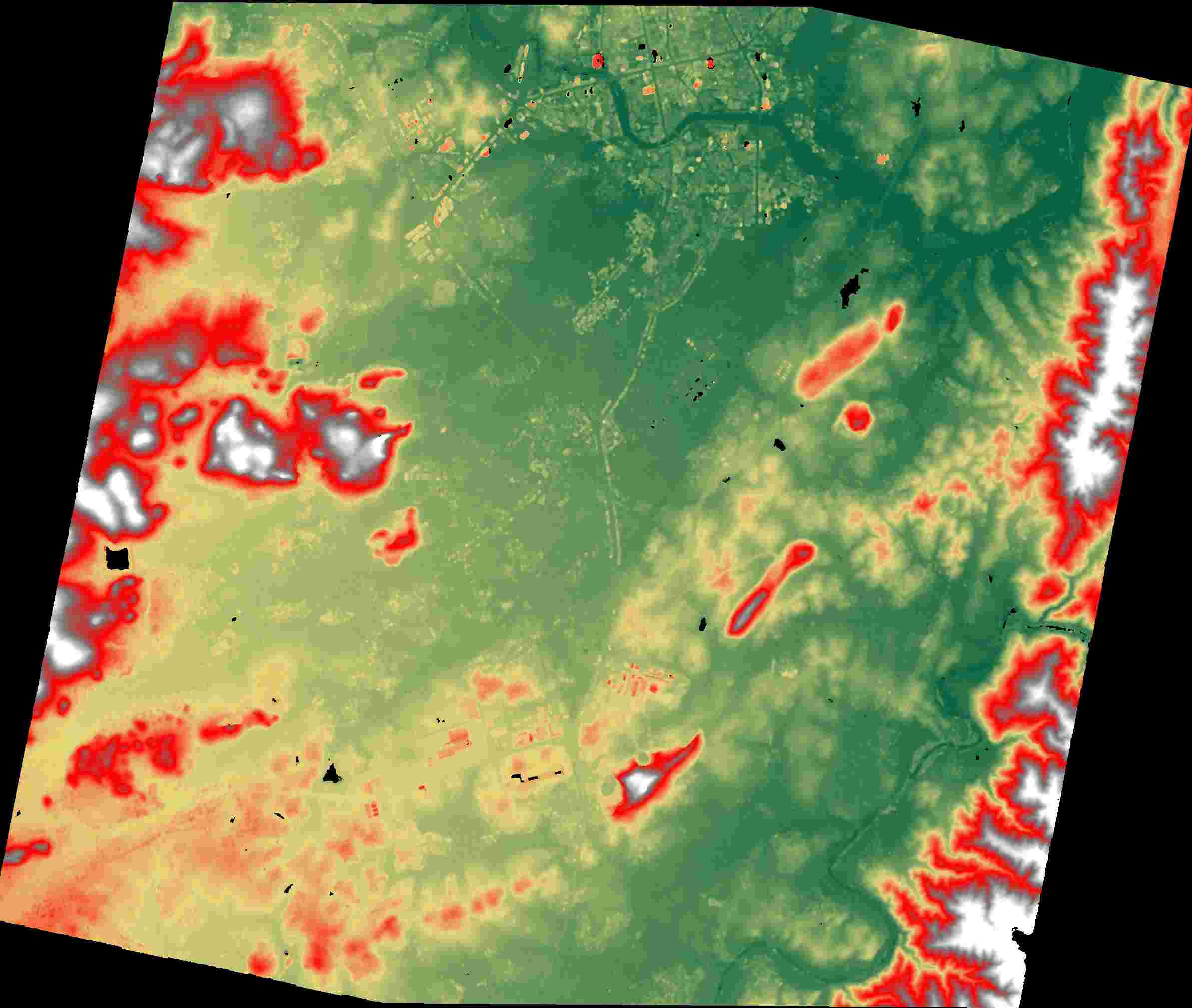
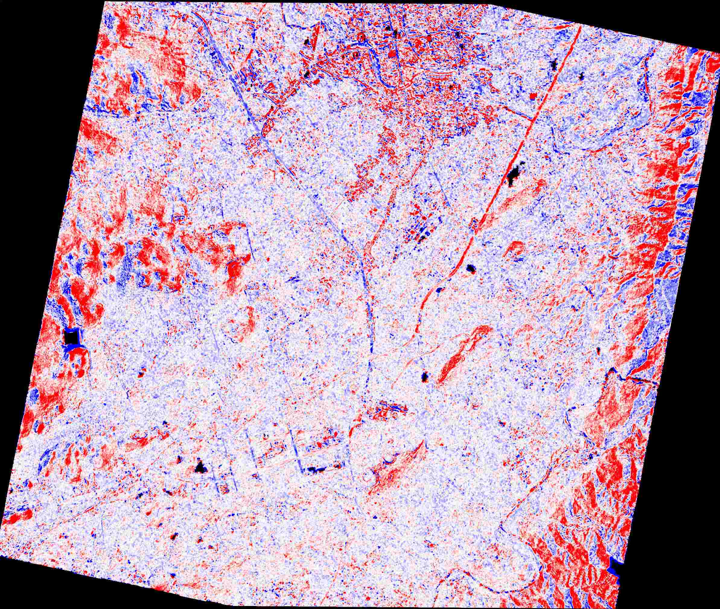
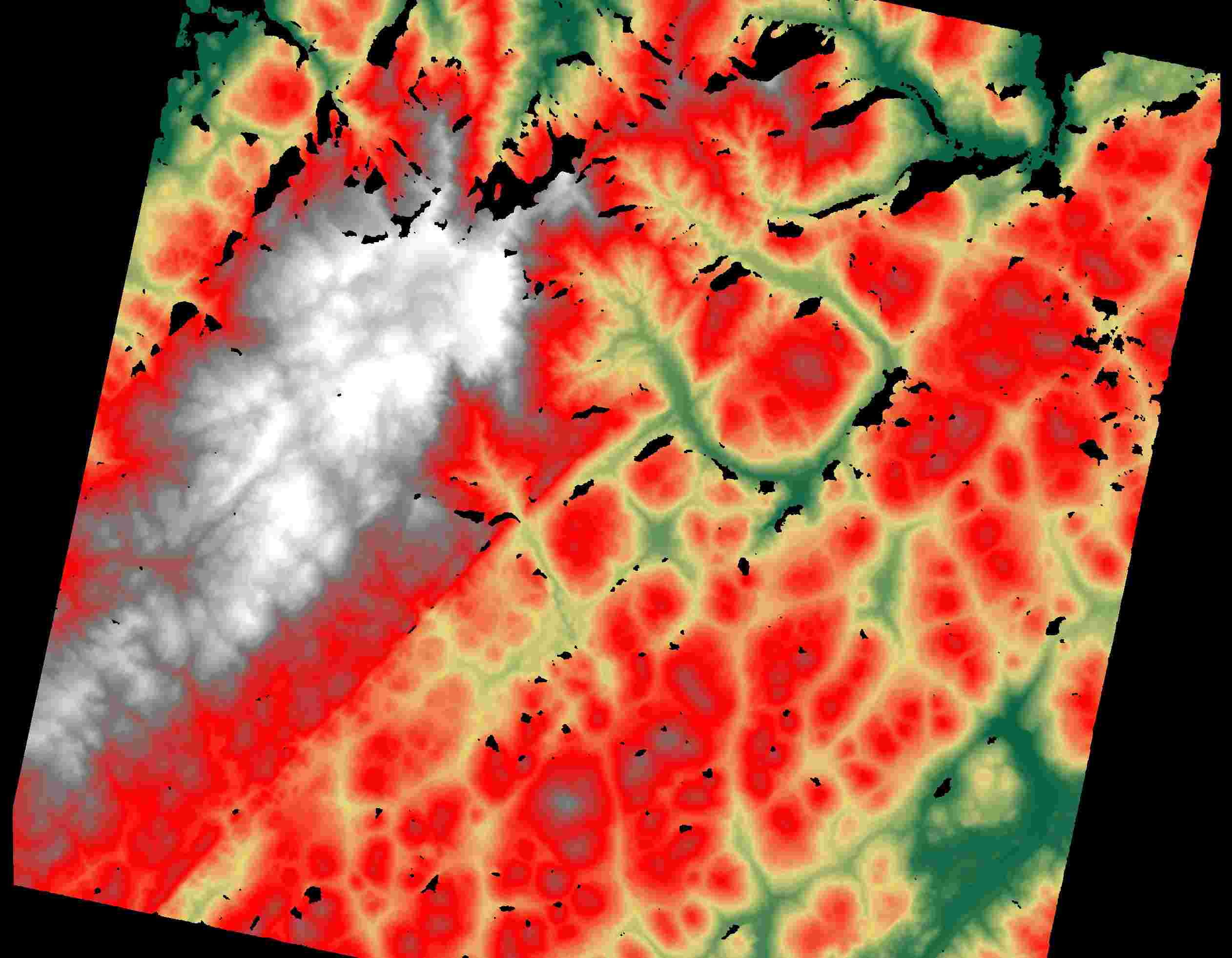
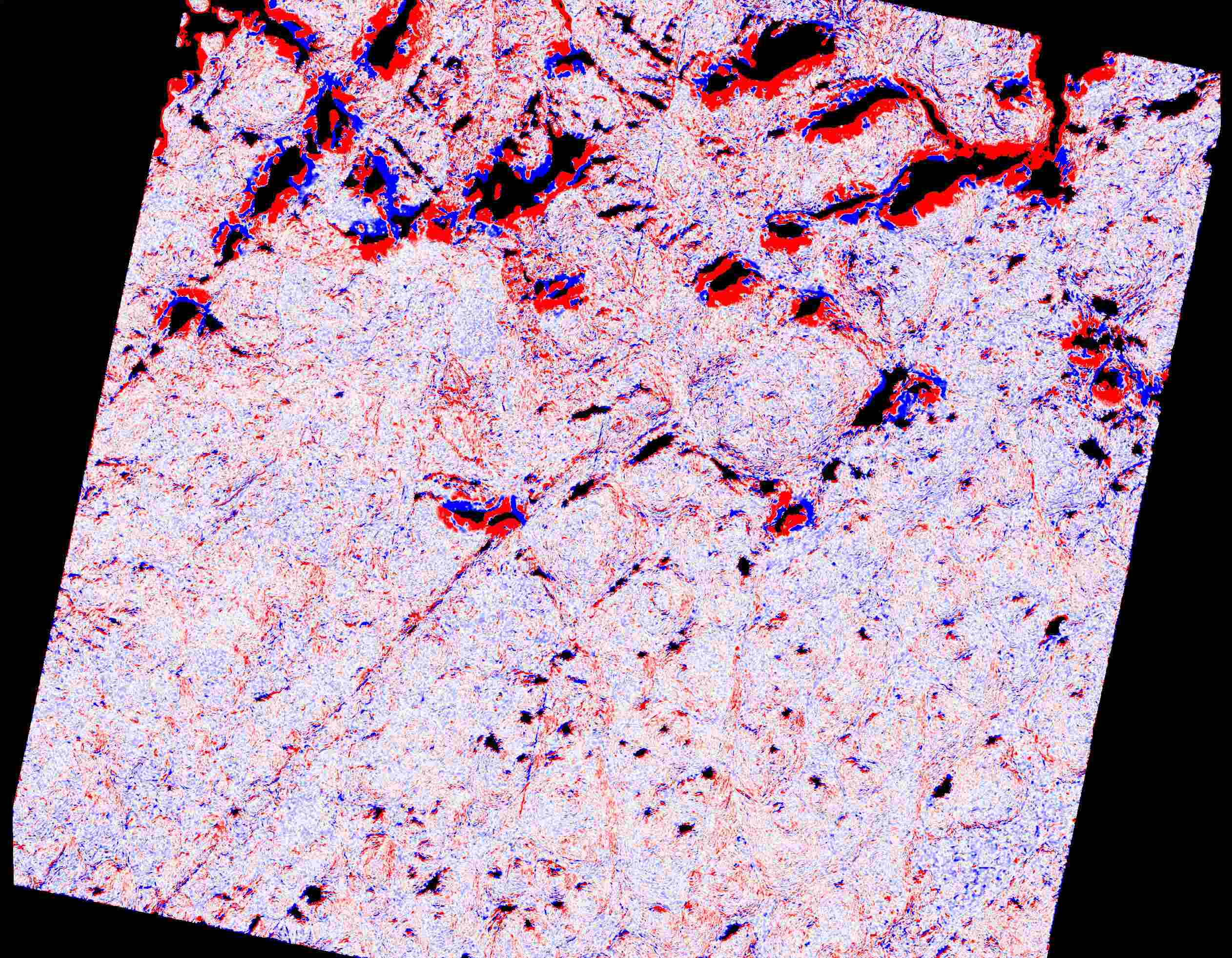
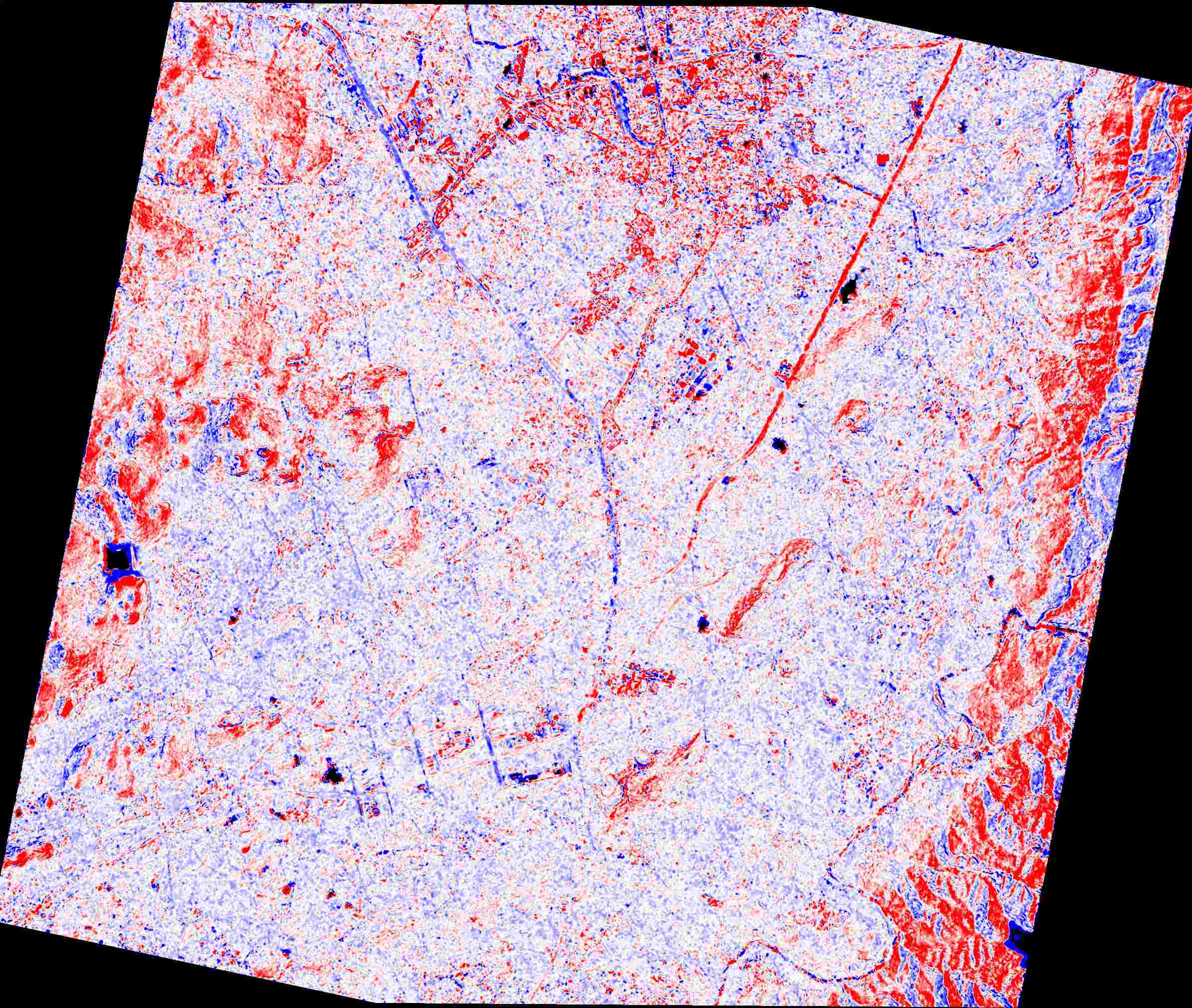
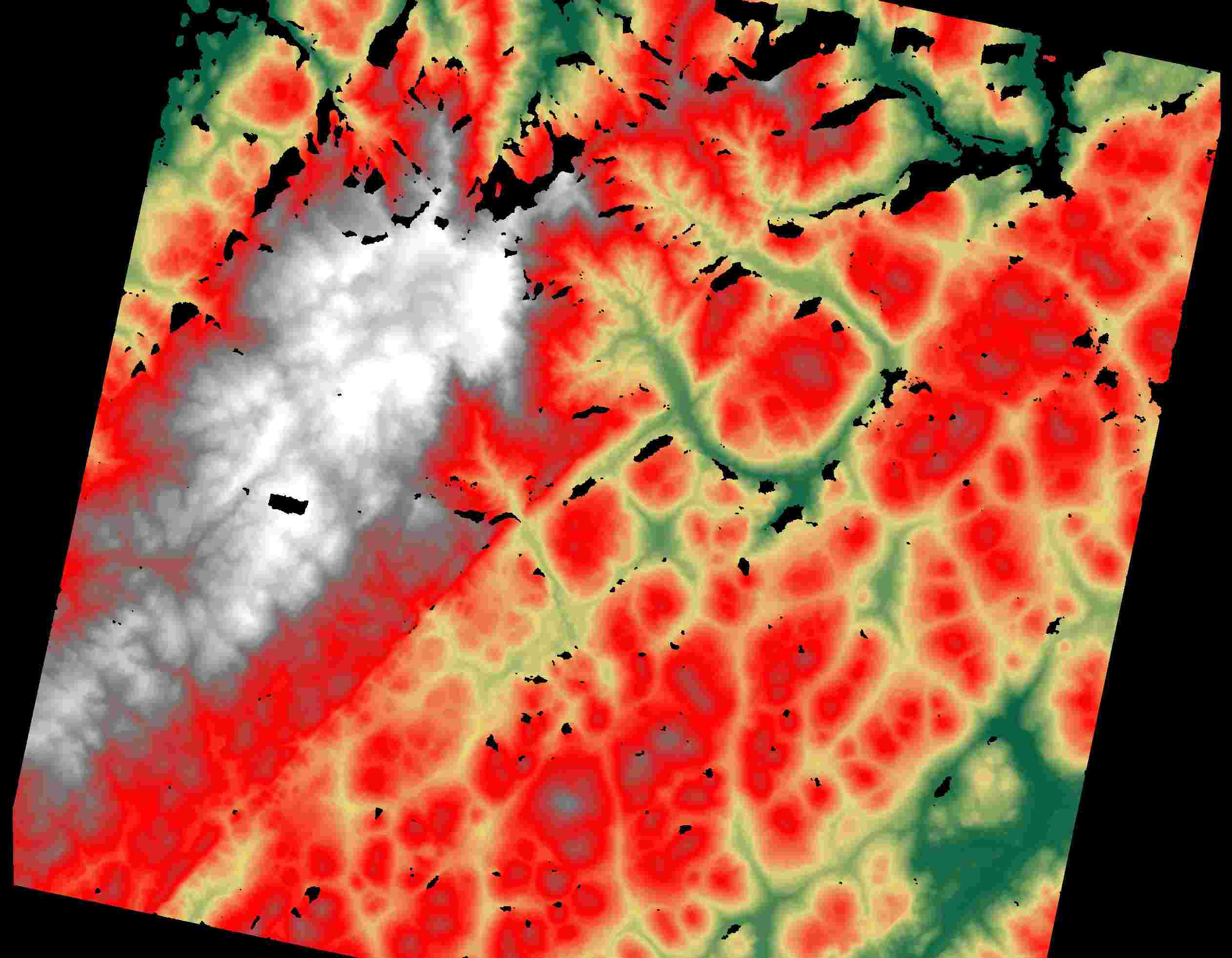
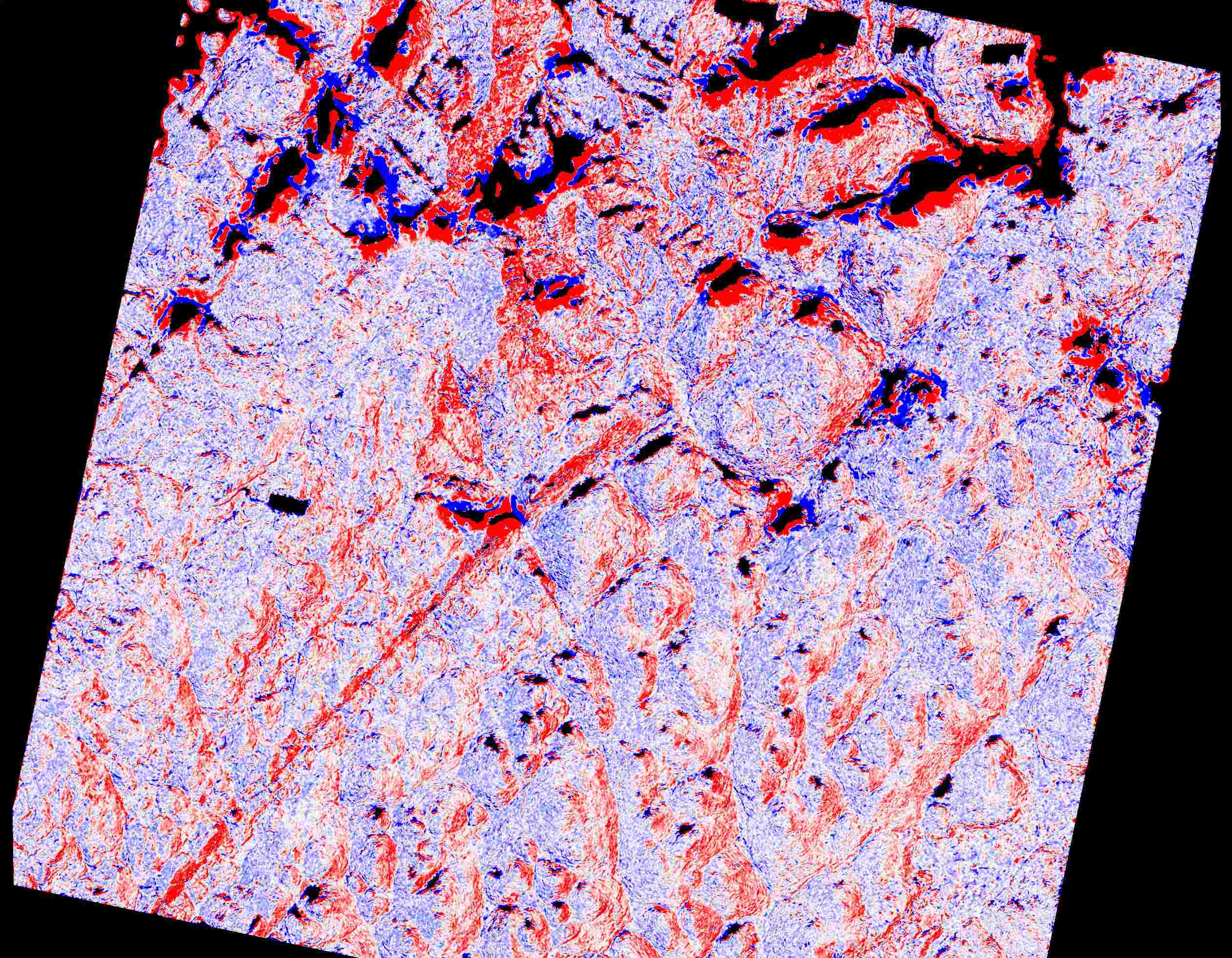
Figure 10: DSM results for different image sizes in the WHU-TLC test set: (a) REPM@5120, (b) REPM@2048, (c) REPM@1024, and (d) REPM@512. The color bar is expressed in units of meters.

5.3 Influence of the polynomial image refinement model

We validated the effectiveness of the polynomial image refinement model on large scale ISPRS-ZY3 satellite images and GF7 satellite images. We compared the homography correction (H-Cor.) and polynomial correction (P-Cor.) for the equivalent error in images of different sizes. According to Table 6, the polynomial correction was more effective than the homography correction, and the effect of the correction was more significant for large-scale satellite images.

Table 6: Equivalent errors of different scale images after homography correction and polynomial correction. All units in the table are pixels (pix.). The two corrections in the table, H-Cor and P-Cor, which resulted in a decrease in error and the largest decrease are shown in bold.

Image Data	Crop Size	Methods	Samp RMSE$\downarrow$	Line RMSE$\downarrow$	RMSE$\downarrow$	Max Error$\downarrow$
ISPRS-ZY3	Full size	Uncorrected	2.457	2.462	3.479	15.402
		H-Cor.	2.505	2.483	3.528	16.855
		P-Cor.	1.912	1.897	2.693	8.156
	10000	Uncorrected	1.302	1.314	1.849	7.622
		H-Cor.	1.315	1.303	1.851	7.738
		P-Cor.	1.166	1.166	1.649	4.871
	5120	Uncorrected	0.616	0.617	0.872	3.112
		H-Cor.	0.617	0.619	0.874	3.271
		P-Cor.	0.597	0.596	0.844	2.450
GF7	Full size	Uncorrected	1.545	1.328	2.038	8.959
		H-Cor.	1.526	1.365	2.047	9.104
		P-Cor.	1.346	1.206	1.807	5.339
	10000	Uncorrected	0.342	0.341	0.483	1.609
		H-Cor.	0.342	0.341	0.483	1.617
		P-Cor.	0.338	0.338	0.478	1.385
	5120	Uncorrected	0.173	0.174	0.246	0.721
		H-Cor.	0.174	0.174	0.246	0.725
		P-Cor.	0.173	0.173	0.245	0.689

In summary, the polynomial image refinement model was found to be more effective based on the metrics of the equivalent error. Subsequently, we evaluated the impact of the polynomial image refinement model on the DSM reconstruction accuracy. The ISPRS-ZY3 data indicated the absolute positioning accuracy calculated by the GCPs, whereas the GF7 data highlighted the accuracy and completeness of the DSM reconstruction. Based on our experimental findings, the addition of a polynomial image refinement model ensured that the reconstruction accuracy did not deteriorate substantially. However, for large images, the reconstruction accuracy and completeness were significantly enhanced.

5.4 Future and outlook

The 3D reconstruction method of RFM is equivalent to PCM provides new ideas and possibilities for the 3D reconstruction of linear-array satellite images. In this study, the proposed REPM pipeline exhibited excellent potential.

However, weakly textured regions (such as bodies of water) remain a significant challenge for the reconstruction method. For instance, the reconstruction results of high-resolution images were more precise in contour. In contrast, the roofs of buildings were prone to larger holes, as shown in Fig. 5. Although high-resolution images are favorable for including more details in the reconstruction, this causes certain patches in the images to lack texture, which causes the matching computation and depth estimation to fail in weakly textured regions. Low-resolution images reflect the structural information contained in images more effectively Xu et al. (2023). Consequently, it may be worthwhile to introduce a multi-scale reconstruction framework that enhances the reconstruction effect in weakly textured regions. Furthermore, deep learning could be utilized to address the challenge of reconstructing regions with weak textural features and to enhance the precision and comprehensiveness of DSM reconstruction.

Although we can process VHR images with sizes up to $5120\times 5120$ pixel, satellite images are generally large. If they are cropped (especially considering the overlap), the number of images, the memory they would occupy, and the time they would take to process would all increase exponentially. The number and size of the images determine the efficiency of the pipeline for a given input. Therefore, it is imperative to enhance the pipeline framework and increase the number of parallel operations to improve the operational efficiency of the pipeline.

In addition, because we determined the optimal image processing size based on the equivalent error, in the future we aim to create an adaptable model for choosing the most suitable image size.

6 Conclusion

In this study, we proposed an REPM pipeline for large-scale satellite CCD imagery. The pipeline is equipped with an equivalent pinhole model that converts the RFM to the PCM and a polynomial image refinement model that back-calculates the polynomial correction function to remap the image based on the least squares method. The experimental results showed that the REPM pipeline outperformed the state-of-the-art pipelines on four satellite image datasets. In addition, we assessed the effectiveness of the polynomial image refinement model in enhancing the precision of the DSM reconstruction for large-scale images. This model can be used for 3D reconstruction of large-scale CCD imagery. However, the model has many limitations, such as weak texture region processing methods and low efficiency in handling large-scale satellite images. In the future, we intend to further improve our pipeline by significantly enhancing the stereo matching of low-texture regions and increasing the reconstruction efficiency.

References

- Agisoft (2023) Agisoft, 2023. Agisoft metashape [www document]. URL https://www.agisoft.com/, Last accessed on 2023-9-18.
- BAESystem (2023) BAESystem, 2023. Socet set [www document]. URL https://www.geospatialexploitationproducts.com/content/socet-set-v56/modules/, Last accessed on 2023-10-20.
- Beyer et al. (2018) Beyer, R.A., Alexandrov, O., McMichael, S., 2018. The ames stereo pipeline: Nasa’s open source software for deriving and processing terrain data. Earth and Space Science. 5, 537.0–548.0.
- Bleyer et al. (2011) Bleyer, M., Rhemann, C., Rother, C., 2011. Patchmatch stereo - stereo matching with slanted support windows. in: British Machine Vision Conference , pp. 1–11.
- Bosch et al. (2019) Bosch, M., Foster, K., Christie, G., Wang, S., Hager, G.D., Brown, M., 2019. Semantic stereo for incidental satellite images, in: 2019 IEEE Winter Conference on Applications of Computer Vision (WACV), pp. 1524–1532. doi:10.1109/WACV.2019.00167.
- Bosch et al. (2016) Bosch, M., Kurtz, Z., Hagstrom, S., Brown, M., 2016. A multiple view stereo benchmark for satellite imagery, in: 2016 IEEE Applied Imagery Pattern Recognition Workshop (AIPR), pp. 1–9. doi:10.1109/AIPR.2016.8010543.
- Bosch et al. (2017) Bosch, M., Leichtman, A., Chilcott, D., Goldberg, H., Brown, M., 2017. Metric evaluation pipeline for 3d modeling of urban scenes. The International Archives of the Photogrammetry, Remote Sensing and Spatial Information Sciences XLII-1/W1, 239–246. URL: https://isprs-archives.copernicus.org/articles/XLII-1-W1/239/2017/, doi:10.5194/isprs-archives-XLII-1-W1-239-2017.
- Catalyst (2023) Catalyst, 2023. Catalyst professional [www document]. URL https://catalyst.earth/products/catalyst-pro/, Last accessed on 2023-9-18.
- Facciolo et al. (2015) Facciolo, G., de Franchis, C., Meinhardt, E., 2015. Mgm: A significantly more global matching for stereovision. in: British Machine Vision Conference , pp. 90.1–90.12.
- Facciolo et al. (2017) Facciolo, G., de Franchis, C., Meinhardt-Llopis, E., 2017. Automatic 3d reconstruction from multi-date satellite images. In: Proceedings of the IEEE Conference on Computer Vision and Pattern Recognition Workshops. , pp. 1542–1551.
- Factory (2023) Factory, P., 2023. Pixel factory [www document]. URL https://www.intelligence-airbusds.com/imagery/pixel-factory/, Last accessed on 2023-10-20.
- Felzenszwalb and Huttenlocher (2004) Felzenszwalb, P., Huttenlocher, D., 2004. Efficient belief propagation for early vision, in: Proceedings of the 2004 IEEE Computer Society Conference on Computer Vision and Pattern Recognition, 2004. CVPR 2004., pp. I–I. doi:10.1109/CVPR.2004.1315041.
- de Franchis et al. (2014a) de Franchis, C., Meinhardt-Llopis, E., Michel, J., Morel, J.M., Facciolo, G., 2014a. An automatic and modular stereo pipeline for pushbroom images. ISPRS Annals of the Photogrammetry, Remote Sensing and Spatial Information Sciences II-3, 49–56. URL: https://isprs-annals.copernicus.org/articles/II-3/49/2014/, doi:10.5194/isprsannals-II-3-49-2014.
- de Franchis et al. (2014b) de Franchis, C., Meinhardt-Llopis, E., Michel, J., Morel, J.M., Facciolo, G., 2014b. On stereo-rectification of pushbroom images, in: 2014 IEEE International Conference on Image Processing (ICIP), pp. 5447–5451. doi:10.1109/ICIP.2014.7026102.
- Gao et al. (2021) Gao, J., Liu, J., Ji, S., 2021. Rational polynomial camera model warping for deep learning based satellite multi-view stereo matching, in: 2021 IEEE/CVF International Conference on Computer Vision (ICCV), pp. 6128–6137. doi:10.1109/ICCV48922.2021.00609.
- Gao et al. (2023) Gao, J., Liu, J., Ji, S., 2023. A general deep learning based framework for 3d reconstruction from multi-view stereo satellite images. ISPRS Journal of Photogrammetry and Remote Sensing. 195, 446–461. URL: https://www.sciencedirect.com/science/article/pii/S0924271622003276, doi:https://doi.org/10.1016/j.isprsjprs.2022.12.012.
- Gong and Fritsch (2018) Gong, K., Fritsch, D., 2018. Point cloud and digital surface model generation from high resolution multiple view stereo satellite imagery. The International Archives of the Photogrammetry, Remote Sensing and Spatial Information Sciences. XLII-2, 363–370. URL: https://isprs-archives.copernicus.org/articles/XLII-2/363/2018/, doi:10.5194/isprs-archives-XLII-2-363-2018.
- Grodecki and Dial (2003) Grodecki, J., Dial, G., 2003. Block adjustment of high-resolution satellite images described by rational polynomials. Photogrammetric engineering and remote sensing. 69, 59–68.
- Gómez et al. (2023) Gómez, A., Randall, G., Facciolo, G., Grompone von Gioi, R., 2023. Improving the pair selection and the model fusion steps of satellite multi-view stereo pipelines, in: 2023 IEEE/CVF Winter Conference on Applications of Computer Vision (WACV), pp. 6333–6342. doi:10.1109/WACV56688.2023.00628.
- Hirschmuller (2005) Hirschmuller, H., 2005. Accurate and efficient stereo processing by semi-global matching and mutual information, in: 2005 IEEE Computer Society Conference on Computer Vision and Pattern Recognition (CVPR’05), pp. 807–814 vol. 2. doi:10.1109/CVPR.2005.56.
- ISPRS (2018) ISPRS, 2018. Isprs data sets: Zy-3 [www document]. URL https://www.isprs.org/data/zy-3/Default-HongKong-StMaxime.aspx.
- Jannati et al. (2018) Jannati, M., Valadan Zoej, M.J., Mokhtarzade, M., 2018. A novel approach for epipolar resampling of cross-track linear pushbroom imagery using orbital parameters model. ISPRS Journal of Photogrammetry and Remote Sensing. 137, 1–14. URL: https://www.sciencedirect.com/science/article/pii/S092427161830008X, doi:https://doi.org/10.1016/j.isprsjprs.2018.01.008.
- Leica (2023) Leica, 2023. Erdas imagine lps [www document]. URL https://hexagon.com/products/erdas-imagine/, Last accessed on 2023-9-18.
- Liao et al. (2022) Liao, P., Chen, G., Zhang, X., Zhu, K., Gong, Y., Wang, T., Li, X., Yang, H., 2022. A linear pushbroom satellite image epipolar resampling method for digital surface model generation. ISPRS Journal of Photogrammetry and Remote Sensing. 190, 56–68. URL: https://www.sciencedirect.com/science/article/pii/S0924271622001496, doi:https://doi.org/10.1016/j.isprsjprs.2022.05.010.
- Loghman and Kim (2013) Loghman, M., Kim, J., 2013. Sgm-based dense disparity estimation using adaptive census transform, in: 2013 International Conference on Connected Vehicles and Expo (ICCVE), pp. 592–597. doi:10.1109/ICCVE.2013.6799860.
- Marí et al. (2019) Marí, R., de Franchis, C., Meinhardt-Llopis, E., Facciolo, G., 2019. To bundle adjust or not: A comparison of relative geolocation correction strategies for satellite multi-view stereo, in: 2019 IEEE/CVF International Conference on Computer Vision Workshop (ICCVW), pp. 2188–2196. doi:10.1109/ICCVW.2019.00274.
- Michel et al. (2020) Michel, J., Sarrazin, E., Youssefi, D., Cournet, M., Buffe, F., Delvit, J.M., Emilien, A., Bosman, J., Melet, O., L’Helguen, C., 2020. A new satellite imagery stereo pipeline designed for scalability, robustness and performance. ISPRS Annals of the Photogrammetry, Remote Sensing and Spatial Information Sciences. V-2-2020, 171–178. URL: https://isprs-annals.copernicus.org/articles/V-2-2020/171/2020/, doi:10.5194/isprs-annals-V-2-2020-171-2020.
- nFrames (2023) nFrames, E., 2023. Sure software [www document]. URL https://geo-matching.com/products/sure-software-empowering-photogrammetry, Last accessed on 2023-10-20.
- Poullis (2020) Poullis, C., 2020. Large-scale urban reconstruction with tensor clustering and global boundary refinement. IEEE Transactions on Pattern Analysis and Machine Intelligence 42, 1132–1145. doi:10.1109/TPAMI.2019.2893671.
- Qin (2016) Qin, R., 2016. Rpc stereo processor (rsp) - a software package for digital surface model and orthophoto generation from satellite stereo imagery. ISPRS Annals of the Photogrammetry, Remote Sensing and Spatial Information Sciences III-1, 77–82. URL: https://isprs-annals.copernicus.org/articles/III-1/77/2016/, doi:10.5194/isprs-annals-III-1-77-2016.
- Rupnik et al. (2017) Rupnik, E., Daakir, M., Deseilligny, M.P., 2017. Micmac - a free, open-source solution for photogrammetry. Open Geospatial Data, Software and Standards. 2, 14.
- Rupnik et al. (2018) Rupnik, E., Pierrot-Deseilligny, M., Delorme, A., 2018. 3d reconstruction from multi-view vhr-satellite images in micmac. ISPRS Journal of Photogrammetry and Remote Sensing. 139, 201–211. URL: https://www.sciencedirect.com/science/article/pii/S0924271618300819, doi:https://doi.org/10.1016/j.isprsjprs.2018.03.016.
- Schönberger and Frahm (2016) Schönberger, J.L., Frahm, J.M., 2016. Structure-from-motion revisited, in: Conference on Computer Vision and Pattern Recognition (CVPR).
- Schönberger et al. (2016) Schönberger, J.L., Zheng, E., Pollefeys, M., Frahm, J.M., 2016. Pixelwise view selection for unstructured multi-view stereo, in: European Conference on Computer Vision (ECCV).
- Stucker et al. (2022) Stucker, C., Ke, B., Yue, Y., Huang, S., Armeni, I., Schindler, K., 2022. Implicity: City modeling from satellite images with deep implicit occupancy fields. ISPRS Annals of the Photogrammetry, Remote Sensing and Spatial Information Sciences. V-2-2022, 193–201. URL: https://isprs-annals.copernicus.org/articles/V-2-2022/193/2022/, doi:10.5194/isprs-annals-V-2-2022-193-2022.
- Tang and Tan (2019) Tang, C., Tan, P., 2019. Ba-net: Dense bundle adjustment network. in: International Conference on Learning Representations abs/1806.04807.
- Tao and Hu (2000) Tao, C., Hu, Y., 2000. Investigation on the rational function model. ASPRS 2000 Annual Conference Proceedings, Washington D.C. .
- Tao and Hu (2001) Tao, C., Hu, Y., 2001. A comprehensive study of the rational function model for photogrammetric processing. Photogrammetric Engineering and Remote Sensing. 67, 1347–1357.
- Tao and Hu (2002) Tao, C., Hu, Y., 2002. 3d reconstruction methods based on rational function model. Photogrammetric Engineering and Remote Sensing. 68, 705–714.
- Tatar and Arefi (2019) Tatar, N., Arefi, H., 2019. Stereo rectification of pushbroom satellite images by robustly estimating the fundamental matrix. International journal of remote sensing. 40, 8879–8898.
- Wang and Frahm (2017) Wang, K., Frahm, J.M., 2017. Fast and accurate satellite multi-view stereo using edge-aware interpolation, in: 2017 International Conference on 3D Vision (3DV), pp. 365–373. doi:10.1109/3DV.2017.00049.
- Wang et al. (2022) Wang, P., Shi, L., Chen, B., Hu, Z., Qiao, J., Dong, Q., 2022. Pursuing 3-d scene structures with optical satellite images from affine reconstruction to euclidean reconstruction. IEEE Transactions on Geoscience and Remote Sensing 60, 1–14. doi:10.1109/TGRS.2022.3213546.
- Xia et al. (2020) Xia, Y., d’Angelo, P., Tian, J., Reinartz, P., 2020. Dense matching comparison between classical and deep learning based algorithms for remote sensing data. The International Archives of the Photogrammetry, Remote Sensing and Spatial Information Sciences. XLIII-B2-2020, 521–525. URL: https://isprs-archives.copernicus.org/articles/XLIII-B2-2020/521/2020/, doi:10.5194/isprs-archives-XLIII-B2-2020-521-2020.
- Xu et al. (2023) Xu, Q., Kong, W., Tao, W., Pollefeys, M., 2023. Multi-scale geometric consistency guided and planar prior assisted multi-view stereo. IEEE Transactions on Pattern Analysis and Machine Intelligence. 45, 4945–4963. doi:10.1109/TPAMI.2022.3200074.
- Zhang et al. (2019a) Zhang, F., Prisacariu, V., Yang, R., Torr, P.H., 2019a. Ga-net: Guided aggregation net for end-to-end stereo matching, in: 2019 IEEE/CVF Conference on Computer Vision and Pattern Recognition (CVPR), pp. 185–194. doi:10.1109/CVPR.2019.00027.
- Zhang et al. (2019b) Zhang, K., Snavely, N., Sun, J., 2019b. Leveraging vision reconstruction pipelines for satellite imagery, in: 2019 IEEE/CVF International Conference on Computer Vision Workshop (ICCVW), pp. 2139–2148. doi:10.1109/ICCVW.2019.00269.
- Zhao et al. (2023) Zhao, L., Wang, H., Zhu, Y., Song, M., 2023. A review of 3d reconstruction from high-resolution urban satellite images. International Journal of Remote Sensing. 44, 713–748.