On the entropy of a stealth vector-tensor black hole

Abstract

We apply Wald’s formalism to a Lagrangian within generalised Proca gravity that admits a Schwarzschild black hole with a non-trivial vector field. The resulting entropy differs from that of the same black hole in General Relativity by a logarithmic correction modulated by the only independent charge of the vector field. We find conditions on this charge to guarantee that the entropy is a non-decreasing function of the black hole area, as is the case in GR. If this requirement is extended to black hole mergers, we find that for Planck scale black holes, a non-decreasing entropy is possible only if the area of the final black hole is several times larger than the initial total area of the merger. Finally, we discuss some implications of the vector Galileon entropy from the point of view of entropic gravity.

I Introduction

Since its conception, the theory of General Relativity (GR) proposed by Albert Einstein in 1917, has been subject to a variety of observational tests. In the realm of cosmology, the concordance model is $\Lambda$CDM, which is based on GR. This model is in agreement with most cosmological observations that constrain the evolution and properties of the background spacetime, the matter fields and their perturbations [1]. In addition, recent astrophysical observations show compatibility with the properties of the spacetime around black holes predicted by GR [2, 3, 4, 5]. In this scenario, alternative theories of gravity need to predict cosmic and astrophysical solutions that are similar to the spacetimes predicted by GR in order to be considered viable. Several theories of modified gravity predict solutions that deviate parametrically from GR, and these deviations can be used to put constraints on the parameter(s) of the theory by contrasting their predictions to common cosmological and astrophysical direct or indirect observables, such as luminosity distance, Hubble parameter evolution, structure formation, deflection of light and angular diameter of black hole shadows. However, some other theories of modified gravity predict solutions where the metric coincides exactly with GR solutions even though there is a non-trivial profile for the additional fields of the theory. These are known in the literature as stealth solutions (e.g. [6, 7, 8, 9, 10, 11, 12, 13, 14, 15]). Models with this type of solutions can be more difficult to rule out as alternative theories of gravity, for instance, they can evade solar system constraints. Amongst the possibilities to discriminate these theories, one could consider a direct coupling between the additional fields and matter, or study perturbations. Indeed, at the perturbative level, couplings between the extra fields and matter can appear automatically, as shown in [16] for a scalar-tensor model. Another possibility recently studied in the context of degenerate higher order scalar-tensor theories of gravity, is to introduce a small detuning of the degeneracy conditions, this is known as the scordatura mechanism (e.g. [17]). In this work we explore yet another possibility, namely, we analyse the Wald entropy of the black hole, which we expect to differ from the entropy of a GR Schwarzschild black hole since, even though the metric is the same, the Lagrangian is not the same as in GR and the vector field is not trivial. In particular, we work with a model that belongs to generalised Proca theories, also known as vector Galileons, a type of theories that might be relevant for explaining the accelerated expansion of the universe [18, 19], and have been shown to predict a rich phenomenology for compact objects [10, 20, 9, 8, 21, 22, 23, 24, 25]. We study the Wald entropy of this black hole, which turns out to be the Bekenstein-Hawking entropy with a logarithmic correction introduced by the vector field. We analyse the consequences of this correction in two different scenarios. The first one is related to the area theorem of GR [26], and motivated by recent observational support to this theorem [27] using gravitational waves. The second scenario we analyse is in the context of the entropic gravity derivation of a modified Newtonian potential [28, 29] and a modified Friedmann equation [30, 31, 32].

This work is organised as follows. In Sec. II we present the vector Galileon model and black hole solution under study. In Sec. III we review the basics of Wald formalism and its application to the Schwarzschild black hole in GR, and then we apply the formalism to the Schwarzschild black hole in VG and discuss some properties of the resulting entropy. In Sec. IV we explore the implications of the VG modified entropy for the area theorem and for astrophysical and cosmological applications of entropic gravity. Finally, Sec. V is devoted to conclusions.

II Black holes in vector-tensor gravity

We focus on the theory of vector-tensor gravity known as generalized Proca theory, also referred to as vector galileons due to the similarity between their construction and that of scalar galileons. As in Proca theory, the longitudinal mode of the vector field becomes dynamical as a consequence of breaking the Abelian symmetry. However, in generalised Proca the Abelian symmetry is broken not only by the mass term of the vector field but also by non–minimal couplings with gravity. This characteristic offers a way around Bekenstein’s no-go theorem, which applies to black holes in theories where the Abelian symmetry is broken by a mass term. This was exploited in [10] to show that the Schwarzschild spacetime is a solution in a sector of generalised Proca theory. More general black hole solutions have been reported in [20, 9, 8, 21, 22, 23, 24, 25]. In this work, we use the stealth Schwarzschild solution that is obtained in the model described by

$$S=\int d^{4}x\sqrt{-g}\left[{\frac{1}{16\pi}}\,R-\frac{1}{4}{F_{ab}F^{ab}}+\gamma\,G_{ab}A^{a}A^{b}\right],$$ (1)

where the electromagnetic tensor $F_{ab}=\partial_{a}A_{b}-\partial_{b}A_{a}$ is constructed out of the 4–potential $A_{b}$ and $R$ is the Ricci scalar of the metric $g_{ab}$. The coupling of the 4–potential $A_{b}$ with the Einstein tensor $G_{ab}$, weighted by the dimensionless constant $\gamma$, breaks the Abelian symmetry of the Lagrangian and turns on the longitudinal mode of the vector field in such a way that the theory propagates five degrees of freedom [18]. Considering a spherically symmetric ansatz,

$$ds^{2} = -f(r)dt^{2}+h(r)^{-1}dr^{2}+r^{2}d\theta^{2}+r^{2}\sin^{2}\theta d\varphi^{2},$$

$$A_{b} = (A_{0}(r),A_{1}(r),0,0),$$ (2)

the equations of motion for the system can be expressed as

$$0 = \gamma A_{1}\left[h-f(f+rf^{\prime})^{-1}\right],$$ (3a)

$$0 = {\frac{f}{4\pi}}(h-1)+hr^{2}{A_{0}^{\prime}}^{2}+2{\frac{1}{8\pi}}rhf^{\prime}$$ (3b)

$$+\gamma\left[2A_{0}^{2}(h-1)+2fh(3h-1)A_{1}^{2}+8{A_{0}}hr{A_{0}}^{\prime}-2A_{0}^{2}hr\frac{f^{\prime}}{f}+6h^{2}A_{1}^{2}rf^{\prime}\right],$$

$$0 = {\frac{f}{4\pi}}(1-h-rh^{\prime})-hr^{2}{A_{0}^{\prime}}^{2}$$ (3c)

$$+\gamma\left[2A_{0}^{2}\left(h-1+rh^{\prime}\right)-2fh{A_{1}}\left({A_{1}}\left(h+1+3rh^{\prime}\right)+4hr{A_{1}^{\prime}}\right)\right],$$

$$0 = 4{A_{0}}\gamma\left(h-1+rh^{\prime}\right)-r\left[{A_{0}^{\prime}}\left(hr\frac{f^{\prime}}{f}-4h-rh^{\prime}\right)-2hr{A_{0}^{\prime\prime}}\right],$$ (3d)

where a prime indicates derivative with respect to the radial coordinate. The radial component of the vector field, $A_{1}(r)$, is associated with the longitudinal polarization of the vector, which has an important role in our scenario that breaks the Abelian symmetry. If $\gamma=0$ or $A_{1}(r)=0$, Eq. (3a) is identically satisfied, and the remaining equations lead to the Reissner-Nördstrom solution. On the other hand, if $\gamma\neq 0$ and $A_{1}(r)\neq 0$, the first equation fully determines $h(r)$ in terms of $f(r)$. Asymptotically flat solutions for arbitrary values of $\gamma$ can be found analytically and numerically. However, only for $\gamma=1/4$ Minkowski spacetime is an exact solution with a non-trivial profile of the vector field. This observation motivates us to set $A_{1}(r)\neq 0$ and $\gamma=1/4$. Under these assumptions, Eqs. (3) lead to the following solutions:

$$f(r) =h(r)\,=\,1-\frac{2M}{r},$$ (4)

$$A_{0}(r) =\frac{Q}{r}+P,$$ (5)

$$A_{1}(r) =\frac{\sqrt{Q^{2}+2\,r\,P(Q+M\,P)}}{r-2M},$$ (6)

where $M$ represents the black hole mass, and $Q,~{}P$ are charges associated to the vector field. In particular, $P$ determines the asymptotic behaviour of $A_{1}(r)$: if $P=0$ then $A_{1}(r)\sim 1/r$, while if $P\neq 0$ then $A_{1}(r)\sim 1/\sqrt{r}$. Furthermore, $P$ also determines the norm of the vector field, which for this solution is a constant, $A_{b}A^{b}=-P^{2}$ . Notice that the metric components, Eq.(4), exactly coincide with the Schwarzschild space-time, thus this is a stealth solution, i.e. it matches a GR counterpart, but with a non-trivial profile for the vector field. In the next sections we explore how the entropy of this black hole mismatches that of a Schwarzschild black hole in General Relativity.

III Wald formalism

In this section we review the notion of black hole entropy as an integral of a Nöether charge, introduced by R. Wald in 1993 [33, 34]. Let us consider an action $I$ given as the integral of a Lagrangian $4$-form $\mathbf{L}$,

$$I=\int\mathbf{L}=\int\boldsymbol{\epsilon}L,$$ (7)

where $\boldsymbol{\epsilon}$ is the canonical volume form on the 4-dimensional manifold. Assuming that the Lagrangian is diffeomorphism covariant, it can be expressed as

$$\mathbf{L}=\mathbf{L}\left(g_{ab},R_{bcde},\nabla_{a_{1}}R_{bcde},\dots,\nabla_{(a_{1}\dots}\nabla_{a_{m})}R_{bcde},\Psi,\nabla_{a_{1}}\Psi,\dots,\nabla_{(a_{1}\dots}\nabla_{a_{m})}\Psi\right),$$ (8)

where the parentheses around indices indicate symmetrization and $\Psi$ represents any dynamical fields with arbitrary index structure, for instance a scalar or a vector field. The first order variation of the Lagrangian can be expressed, after integration by parts, as

$$\delta\mathbf{L}=(\mathbf{E}_{g})^{ab}\delta g_{ab}+\mathbf{E}_{\Psi}\delta\Psi+d\mathbf{\Theta},$$ (9)

where all the variations $\delta\Psi$ of the additional fields are summed over and the boundary term is given by the 3-form $\mathbf{\Theta}$ that depends on the fields, their variations, and their derivatives. The dependency of $\mathbf{\Theta}$ on the variations is only linear. From the requirement that the variation of the action vanishes, the equations of motion are

$$(\mathbf{E}_{g})^{ab}=0,\ \ \ \mathbf{E}_{\Psi}=0$$ (10)

The boundary terms coming from the dependencies of the Lagrangian on the metric and Riemann tensors can be worked out in general [34], so that the 3-form $\mathbf{\Theta}$ can be written as

$$\mathbf{\Theta}=2\mathbf{E}_{R}^{bcd}\nabla_{d}\delta g_{bc}-2(\nabla_{d}\mathbf{E}_{R}^{bcd})\delta g_{bc}+\tilde{\mathbf{\Theta}},$$ (11)

where $\tilde{\mathbf{\Theta}}$ contains the boundary terms associated to the additional fields $\Psi$ and, restricting our attention to Lagrangians that do not depend on derivatives of the Riemann tensor, we have

$$(\mathbf{E}_{R}^{bcd})_{a_{1}a_{2}a_{3}}=\epsilon_{aa_{1}a_{2}a_{3}}\frac{\partial L}{\partial R_{abcd}},$$ (12)

where $\epsilon_{abcd}$ is the Levi–Civita tensor density. Under this simplifying assumption, the components of $\mathbf{\Theta}$ can be expressed as

$$(\mathbf{\Theta})_{a_{1}a_{2}a_{3}}=\epsilon_{aa_{1}a_{2}a_{3}}\left[2\frac{\partial L}{\partial R_{abcd}}\nabla_{d}\delta g_{bc}-2\nabla_{d}\left(\frac{\partial L}{\partial R_{abcd}}\right)\delta g_{bc}+\tilde{\Theta}^{a}\right]\equiv\epsilon_{aa_{1}a_{2}a_{3}}\mathcal{J}^{a}.$$ (13)

For a diffeomorphism invariant theory, considering variations of the fields generated by an infinitesimal vector field $\boldsymbol{\xi}$, there is a $3$-form $\mathbf{J}$ that defines the conserved Nöether current as

$$\mathbf{J}=\mathbf{\Theta}(g,\Psi,\mathcal{L}_{\xi}g,\mathcal{L}_{\xi}\Psi)-\boldsymbol{\xi}\cdot\mathbf{L},$$ (14)

where $\mathbf{\Theta}(g,\Psi,\mathcal{L}_{\xi}g,\mathcal{L}_{\xi}\Psi)$ is obtained from Eq. (13) considering that the variations of the fields are given by their Lie derivatives along the infinitesimal generator of the diffeomorphism, and $\boldsymbol{\xi}\cdot\mathbf{L}$ represents the contraction of the vector field components $\xi^{a}$ with the first index of the Lagrangian 4-form $\mathbf{L}$. It can be shown that $\mathbf{J}$ is a closed form under the condition that the equations of motion are satisfied. In this case, it can be expressed as

$$\mathbf{J}=d\mathbf{Q}.$$ (15)

The 2-form $\mathbf{Q}$ is called the Nöether charge. As shown in [33], when the linearized field equations are satisfied, the variation of the Hamiltonian associated to variations of the fields generated by $\xi^{a}$ is given by

$$\delta\mathcal{H}=\int_{\infty}(\delta\mathbf{Q}-\boldsymbol{\xi}\cdot\boldsymbol{\Theta}),$$ (16)

where integration is performed over a 2-dimensional sphere at infinity. Let us consider static black holes with a bifurcate killing horizon $\Sigma$, i.e., a surface where the killing field vanishes. For the Schwarzschild space-time this surface coincides with the position of the event horizon. In this setup, the first law of thermodynamics derived in [33] (see also [35]) can be expressed as

$$\int_{\infty}(\delta\mathbf{Q}-\boldsymbol{\xi}\cdot\boldsymbol{\Theta})=\int_{\Sigma}(\delta\mathbf{Q}-\boldsymbol{\xi}\cdot\boldsymbol{\Theta}).$$ (17)

Choosing $\boldsymbol{\xi}$ as the timelike killing vector, Eq. (16) gives the change $\delta M$ in the ADM mass of the solution. On the other hand, the right hand side of Eq. (17) is defined as $(\kappa/2\pi)\delta S$, where $S$ is the entropy and $\kappa$ the surface gravity of the solution, related to the temperature by $T=\kappa/2\pi$. Thus, Eq. (17) can be expressed as $\delta M=T\delta S$. From here, one can obtain the black hole entropy.

In order to exemplify the application of Wald formalism, let us review the computation of the entropy for a Schwarzschild black hole in GR. In geometrized units, the components of the Lagrangian 4-form are

$$(\mathbf{L})_{abcd}=\frac{1}{16\pi}\epsilon_{abcd}R={\epsilon_{abcd}L}.$$ (18)

Notice that the factor $1/16\pi$ is included in $L$. Using the symmetry properties of the metric and Riemann tensor, it is straightforward to verify that

$$\frac{\partial L}{\partial R_{abcd}}=\frac{1}{32\pi}\left(g^{ac}g^{bd}-g^{ad}g^{bc}\right).$$ (19)

Therefore, the $\mathcal{J}^{a}$ defined in Eq. (13) reduces to

$$\mathcal{J}^{a}={\frac{1}{16\pi}}\left(g^{ac}g^{bd}-g^{ad}g^{bc}\right)\nabla_{d}\delta g_{bc}={\frac{1}{16\pi}}g^{ad}g^{bc}\left(\nabla_{c}\delta g_{bd}-\nabla_{d}\delta g_{bc}\right).$$ (20)

To construct the 3-form $\boldsymbol{\Theta}$ we need to consider variations of the metric generated by a diffeomorphism, i.e.,

$$\delta g_{bc}=\nabla_{b}\xi_{c}+\nabla_{c}\xi_{b}.$$ (21)

Inserting Eqs. (20,21) in the equation for $\mathbf{J}$, Eq. (14), we get

$$(\mathbf{J})_{ijk} =\frac{1}{8\pi}\epsilon_{ijka}\left[\nabla_{b}\nabla^{[a}\xi^{b]}-\xi_{b}G^{ab}\right],$$ (22)

where the square brackets around the indices represent antisymmetrization and $G^{ab}$ is the Einstein tensor. When the equations of motion of GR in vacuum are satisfied, this tensor vanishes. Therefore, the 2-form Nöether charge $\mathbf{Q}$, defined in Eq. (15) comes from the first term in the previous equation. One can verify that its components

$$(\mathbf{Q})_{ij}=-{\frac{1}{16\pi}}\epsilon_{ijab}\nabla^{a}\xi^{b},$$ (23)

are such that

$$(d\mathbf{Q})_{ijk}=-{\frac{1}{16\pi}}3\nabla_{[i}\left(\epsilon_{jk]ab}\nabla^{a}\xi^{b}\right)=\mathbf{J}_{ijk},$$ (24)

when the equations of motion are satisfied. Now we evaluate $\delta\mathbf{Q}$ for a metric of the form given in Eq. (2). It is important to highlight that, while $\mathbf{Q}$ is constructed for a diffeomorphism, its variations in Eq. (17) are only subject to the condition that they satisfy the linearized equations of motion. We obtain these variations by replacing $f(r)\to f(r)+\delta f(r)$ and $h(r)\to h(r)+\delta h(r)$ in Eq. (2), where $\delta h$ and $\delta f$ are to be specified depending on whether we are evaluating these quantities at infinity or at the Killing horizon $\Sigma$. Thus, we find that the non-vanishing components of $\delta\mathbf{Q}-\boldsymbol{\xi}\cdot\boldsymbol{\Theta}$ are

$$(\delta\mathbf{Q}-\boldsymbol{\xi}\cdot\boldsymbol{\Theta})_{23}=-(\delta\mathbf{Q}-\boldsymbol{\xi}\cdot\boldsymbol{\Theta})_{32}=-{\frac{r}{8\pi}}{}\sqrt{\frac{f(r)}{h(r)}}\delta h(r).$$ (25)

Specializing to a Schwarzschild metric, the variations of $h(r)$ at infinity and at the horizon are, respectively,

$$\delta h(r_{\infty}) =-\frac{2\delta m}{r},$$ (26)

$$\delta h(r_{h}) =-\frac{2m\delta r_{h}}{r_{h}^{2}}.$$ (27)

Thus, the right hand side of Eq. (17) leads to

$$\frac{1}{2}\delta r_{h}=\frac{\kappa}{2\pi}\delta S.$$ (28)

For a Schwarzschild black hole the surface gravity is $\kappa=(4m)^{-1}$. Substituting this into Eq. (28) and rearranging terms, we get

$$\delta S=\delta\left(\frac{A}{4}\right),$$ (29)

where $A$ is the area of a sphere with radius equal to the black hole horizon.

III.1 Wald entropy for a VG Schwarzschild black hole

Let us now apply the Wald formalism described and exemplified in the previous section to the vector Galileon Lagrangian introduced in Eq. (1) and reproduced here for clarity,

$$L=\frac{1}{16\pi}R-\frac{1}{4}F^{ab}F_{ab}+\gamma G_{ab}A^{a}A^{b}.$$ (30)

As discussed in Sec. II, this theory admits a Schwarzschild solution with a non-trivial vector field, given in Eqs. (4,5,6). Since there is an additional field, the term $\tilde{\mathbf{\Theta}}$ in Eq. (11) becomes relevant. Following Eq. (13), this leads to a vector field $\mathcal{J}^{a}$ given by

$$\mathcal{J}^{a}=2\frac{\partial L}{\partial R_{abcd}}\nabla_{d}\delta g_{bc}-2\nabla_{d}\left(\frac{\partial L}{\partial R_{abcd}}\right)\delta g_{bc}+\frac{\partial L}{\partial(\nabla_{a}A_{b})}\delta A_{b}.$$ (31)

Notice that the vector Galileon part of the Lagrangian does not contribute to the third term of $\mathcal{J}^{a}$, but it does contribute to the first two terms through the Riemann tensors contained in $G_{ab}$. As reviewed in the previous section, for the GR Lagrangian one gets

$$\mathcal{J}_{GR}^{a}={\frac{1}{16\pi}}g^{ad}g^{bc}\left(\nabla_{c}\delta g_{bd}-\nabla_{d}\delta g_{bc}\right),$$ (32)

while for the Maxwell and vector Galileon Lagrangian, namely $L_{A}=-\frac{1}{4}F_{ab}F^{ab}+\gamma G_{ab}A^{a}A^{b}$, we have

$$\mathcal{J}^{{a}}_{A}=-F^{{a}{b}}\delta A_{{b}}+\gamma\biggl{\{} -8\pi A^{2}\mathcal{J}_{GR}^{a}+\frac{1}{2}g^{{a}{d}}g^{{b}{c}}\left[\nabla_{{c}}A^{2}\delta g_{{b}{d}}-\nabla_{{d}}A^{2}\delta g_{{b}{c}}\right]+\frac{1}{2}g^{{a}{b}}A^{{d}}A^{{c}}\nabla_{{d}}\delta g_{{c}{b}}-\frac{1}{2}\nabla_{{d}}\left(A^{{a}}A^{{c}}\right)g^{{d}{b}}\delta g_{{c}{b}}$$

$$-\frac{1}{2}g^{{a}{b}}A^{{d}}A^{{c}}\nabla_{{b}}\delta g_{{d}{c}}+\frac{1}{2}\nabla_{{b}}\left(A^{{d}}A^{{c}}\right)g^{{b}{a}}\delta g_{{d}{c}}-\frac{1}{2}g^{{d}{b}}A^{{a}}A^{{c}}\nabla_{{c}}\delta g_{{d}{b}}+\frac{1}{2}\nabla_{{c}}\left(A^{{c}}A^{{a}}\right)g^{{d}{b}}\delta g_{{d}{b}}$$

$$+\frac{1}{2}g^{{d}{b}}A^{{a}}A^{{c}}\nabla_{{b}}\delta g_{{d}{c}}-\frac{1}{2}\nabla_{{d}}\left(A^{{d}}A^{{c}}\right)g^{{a}{b}}\delta g_{{c}{b}}\biggl{\}}.$$ (33)

Then, the components of the 3-form $\boldsymbol{\Theta}$ are given by

$$(\boldsymbol{\Theta})_{a_{1}a_{2}a_{3}}=\epsilon_{aa_{1}a_{2}a_{3}}(\mathcal{J}^{a}_{GR}+\mathcal{J}^{a}_{A}).$$ (34)

When the variations are generated by an infinitesimal diffeomorphism the metric transforms according to Eq. (21), while the vector field transforms as

$$\delta A_{b}=\xi^{d}\nabla_{d}A_{b}+A_{d}\nabla_{b}\xi^{d}.$$ (35)

Inserting this into Eq. (14) we obtain the Nöether current $3$-form $\mathbf{J}=\mathbf{J}_{GR}+\mathbf{J}_{A}$, where $\mathbf{J}_{GR}$ comes from the Einstein-Hilbert Lagrangian $L_{EH}=R/16\pi$ and its components are given by

$$\left(\mathbf{J}_{GR}\right)_{ijk}=-{\frac{1}{8\pi}}\epsilon_{ijka}G^{ab}\xi_{b}+{{\frac{1}{8\pi}}}\epsilon_{ijka}\nabla_{b}\left(\nabla^{[a}\xi^{b]}\right),$$ (36)

and $\mathbf{J}_{A}$ comes from $L_{A}$ and has the components

$$\left(\mathbf{J}_{A}\right)_{ijk}=2\epsilon_{ijka}\nabla_{b}\biggl{\{} \frac{1}{2}F^{ab}A^{d}\xi_{d}-\frac{1}{2}\gamma A^{2}\nabla^{[a}\xi^{b]}+\gamma\nabla^{[a}A^{2}\xi^{b]}+\frac{1}{2}\gamma A^{{d}}A^{[a}\nabla_{{d}}\xi^{b]}-\gamma\nabla_{{d}}\left(A^{{d}}A^{[a}\right)\xi^{b]}$$ (37)

$$-\gamma\nabla^{[a}\left(A^{b]}A^{{d}}\right)\xi_{{d}}-\frac{1}{2}\gamma A^{{d}}A^{[a}\nabla^{b]}\xi_{{d}}\biggl{\}}+\epsilon_{ijka}T^{ab}\xi_{b}+\tilde{\mathbf{E}}_{A},$$

where $\tilde{\mathbf{E}}_{A}$ vanishes when the equation of motion for $A^{b}$ is satisfied, which we assume to be true, and $T^{ab}$ is the energy-momentum tensor resulting from the vector Lagrangian $L_{A}$, i.e.,

$$T^{ab}=-2\left(\frac{\partial L_{A}}{\partial g_{ab}}-\frac{1}{2}g^{ab}L_{A}\right).$$ (38)

Collecting all the terms together we have

$$(\mathbf{J})_{ijk}= -{\frac{1}{8\pi}}\epsilon_{ijka}{\left(G^{ab}-{{8\pi}}T^{ab}\right)}\xi_{b}$$ (39)

$$+2\epsilon_{ijka}\nabla_{b}\biggl{\{}{\frac{1}{16\pi}}\nabla^{[a}\xi^{b]}+\frac{1}{2}F^{ab}A^{d}\xi_{d}-\frac{1}{2}\gamma A^{2}\nabla^{[a}\xi^{b]}+\gamma\nabla^{[a}A^{2}\xi^{b]}$$

$$+\frac{1}{2}\gamma A^{d}A^{[a}\nabla_{d}\xi^{b]}-\gamma\nabla_{d}\left(A^{d}A^{[a}\right)\xi^{b]}-\gamma\nabla^{[a}\left(A^{b]}A^{d}\right)\xi_{d}-\frac{1}{2}\gamma A^{d}A^{[a}\nabla^{b]}\xi_{d}\biggl{\}}.$$

The first term in Eq. (39) vanishes due to the Einstein field equations

$${G^{ab}}=8\pi T^{ab},$$ (40)

therefore, the final form of the Nöether current is

$$(\mathbf{J})_{ijk}= 2\epsilon_{ijka}\nabla_{b}\biggl{\{}{\frac{1}{16\pi}}\nabla^{[a}\xi^{b]}+\frac{1}{2}F^{ab}A^{d}\xi_{d}-\frac{1}{2}\gamma A^{2}\nabla^{[a}\xi^{b]}+\gamma\nabla^{[a}A^{2}\xi^{b]}$$ (41)

$$+\frac{1}{2}\gamma A^{d}A^{[a}\nabla_{d}\xi^{b]}-\gamma\nabla_{d}\left(A^{d}A^{[a}\right)\xi^{b]}-\gamma\nabla^{[a}\left(A^{b]}A^{d}\right)\xi_{d}-\frac{1}{2}\gamma A^{d}A^{[a}\nabla^{b]}\xi_{d}\biggl{\}}.$$

As can be seen from the last expression, the $3-$form $\mathbf{J}$ is the exterior derivative of a $2$-form $\mathbf{Q}$, i.e. $\mathbf{J}=d\mathbf{Q}$, where

$$(\mathbf{Q})_{ij}=-\epsilon_{ijab}\biggl{[} {\frac{1}{16\pi}}\nabla^{a}\xi^{b}+\frac{1}{2}F^{ab}A^{d}\xi_{d}-\frac{1}{2}\gamma A^{2}\nabla^{a}\xi^{b}+\gamma\nabla^{a}A^{2}\xi^{b}+\frac{1}{2}\gamma A^{d}A^{a}\nabla_{d}\xi^{b}$$ (42)

$$-\gamma\nabla_{d}\left(A^{d}A^{a}\right)\xi^{b}-\gamma\nabla^{a}\left(A^{b}A^{d}\right)\xi_{d}-\frac{1}{2}\gamma A^{d}A^{a}\nabla^{b}\xi_{d}\biggl{]}.$$

The other ingredient we need is $\boldsymbol{\xi}\cdot\boldsymbol{\Theta}$, where the 3-form $\boldsymbol{\Theta}$ is given by expression (34). The components of $\boldsymbol{\xi}\cdot\boldsymbol{\Theta}$ are obtained as

$$(\boldsymbol{\xi}\cdot\boldsymbol{\Theta})_{ij}=\epsilon_{ijab}\left[2\frac{\partial L}{\partial R_{cead}}\nabla_{e}\delta g_{cd}-2\nabla_{d}\frac{\partial L}{\partial R_{cade}}\delta g_{ce}+\frac{\partial L}{\partial(\nabla_{a}A_{d})}\delta A_{d}\right]\xi^{b}.$$ (43)

Now that we have $\mathbf{Q}$ and $\boldsymbol{\xi}\cdot\boldsymbol{\Theta}$ , we are ready to construct the variation $\delta\mathbf{Q}-\boldsymbol{\xi}\cdot\boldsymbol{\Theta}$ required by Wald’s formalism in order to obtain the entropy of the Schwarzschild black hole solution with a non-trivial vector field, given in Eqs. (4,5,6) and valid for $\gamma=1/4$. In this setup, and with a timelike Killing vector field, we find the non-vanishing components of $\mathbf{Q}$ and $\boldsymbol{\xi}\cdot\mathbf{\Theta}$ as

$$(\mathbf{Q})_{23}= \,\frac{\sqrt{h}r^{2}\left(f^{\prime}-16\pi A_{0}A_{0}^{\prime}\right)}{16\pi\sqrt{f}}-\gamma\frac{\sqrt{h}r\left[A_{1}^{2}fh\left(rf^{\prime}+2f\right)+A_{0}r\left(4fA_{0}^{\prime}-A_{0}f^{\prime}\right)\right]}{f^{3/2}},$$ (44)

$$(\boldsymbol{\xi}\cdot\mathbf{\Theta})_{23}= \,\frac{1}{2}r\sqrt{\frac{1}{hf^{3}}}\biggl{[}{\frac{1}{16\pi}}f\delta h(4f+rf^{{}^{\prime}})+{\frac{1}{16\pi}}rh(2f\delta f^{{}^{\prime}}-f^{{}^{\prime}}\delta f)+\frac{2}{r}hf\delta A_{0}$$

$$+2\gamma\delta hf\left(P+\frac{Q}{r}\right)^{2}-\frac{2\gamma}{(r-2m)^{2}}(Q^{2}+2mrP^{2}+2rPQ)h^{2}f\delta f\biggl{]}.$$ (45)

Taking the variation of $\mathbf{Q}$ and combining with Eq. (45), we find

$$\int(\delta\mathbf{Q}-\boldsymbol{\xi}\cdot\boldsymbol{\Theta})= -\frac{1}{2}r\delta h-\frac{2\pi r^{2}A_{0}\left[r(\delta f-\delta h)A_{0}^{\prime}+2(r-2m)\delta A_{0}^{\prime}\right]}{r-2m}$$

$$-2\pi\gamma\Bigg{\{}\frac{2r^{2}A_{0}}{(r-2m)^{2}}\bigg{[}3m(\delta f-\delta h)+r\delta h-(r-2m)r\delta f^{\prime}\bigg{]}$$

$$+\frac{2}{r}A_{1}\bigg{[}4(r^{2}+2m^{2}-3mr)\delta A_{1}+rA_{1}\Big{(}3r\delta h-m(\delta f+3\delta h)-r(r-2m)\delta f^{\prime}\Big{)}\bigg{]}$$

$$-\frac{4rA_{0}}{r-2m}\bigg{[}2m\delta A_{0}+r^{2}(\delta f-\delta h)A_{0}^{\prime}+2r(r-2m)\delta A_{0}^{\prime}\bigg{]}+8r^{2}A_{0}^{\prime}\delta A_{0}\Bigg{\}},$$ (46)

where we have evaluated the metric components $f$ and $h$ of the Schwarzschild solution.

In order to evaluate the previous result at asymptotic infinity, we have

$$\delta h(r_{\infty})=\delta f(r_{\infty})=-\frac{2\delta m}{r},$$ (47)

$$\delta A_{0}(r_{\infty})=\delta P+\frac{\delta Q}{r},$$

$$\delta A_{1}(r_{\infty})=\frac{(2mP+Q)(r-2m)r\delta P+(rP+Q)(r-2m)\delta Q+\left[2Q^{2}+4rPQ+rP^{2}(r+2m)\right]\delta m}{(r-2m)^{2}\sqrt{Q^{2}+2rP(mP+Q)}},$$

resulting in

$$\int_{\infty}(\delta\mathbf{Q}-\boldsymbol{\xi}\cdot\boldsymbol{\Theta})={\delta m}-4\pi{\delta P}mP+4\pi{\delta Q}P.$$ (48)

Now, for evaluating the variation at $r=r_{h}$, we have

$$\delta h(r_{h})=\delta f(r_{h})=-\frac{2m\delta r_{h}}{r_{h}^{2}},$$ (49)

$$\delta A_{0}(r_{h})=\frac{Q\delta r_{h}}{r_{h}^{2}},$$

$$\delta A_{1}(r_{h})=\frac{\left[2m^{2}P^{2}+2mPQ+Q^{2}+P(mP+Q)r_{h}\right]\delta r_{h}}{(r_{h}-2m)^{2}\sqrt{Q^{2}+2r_{h}P(mP+Q)}},$$

and therefore

$$\int_{\Sigma}(\delta\mathbf{Q}-\boldsymbol{\xi}\cdot\boldsymbol{\Theta})= \frac{m\delta r_{h}}{r_{h}}+\frac{2\pi{\delta r}_{h}\left[Pr_{h}(mP+6{Q})+8{Q}^{2}\right]}{r_{h}^{2}}.$$ (50)

Analyzing Eqs. (48) and (50) under the condition $r_{h}=2m$ imposed by the black hole metric, we find that if $P=2(3+\sqrt{13})Q/r_{h}$ and $\delta Q=0$, then

$$\int_{\infty}(\delta\mathbf{Q}-\boldsymbol{\xi}\cdot\boldsymbol{\Theta})=\int_{\Sigma}(\delta\mathbf{Q}-\boldsymbol{\xi}\cdot\boldsymbol{\Theta}),$$ (51)

i.e., the first law of black hole thermodynamics proposed by Wald is satisfied. The conditions on the vector charges $P$ and $Q$ are interpreted in the following way: the relation between $P,Q$ and $r_{h}$ tells us that not all three charges are independent, something that had been pointed out before for vector galileons [25, 36]. The condition $\delta Q=0$ tells us that the non-constant part of the vector field component $A_{0}$ is screened from spacetime not only at the background level (i.e., $Q$ does not appear in the metric) but also at the level of perturbations needed to obtain the first law of black hole thermodynamics.

Now we can construct the entropy of the Schwarzschild black hole in the vector-tensor theory (30). By definition,

$$\int_{\Sigma}(\delta\mathbf{Q}-\boldsymbol{\xi}\cdot\boldsymbol{\Theta})=\frac{\kappa}{2\pi}\delta S=T\delta S,$$ (52)

where $\kappa$ is the surface gravity. Since the black hole is Schwarzschild, we have $T=(4\pi r_{h})^{-1}$, and using Eq. (51) we get

$$\delta S=4\pi r_{h}\left[\frac{\delta r_{h}}{2}+\frac{16\pi\left(3\sqrt{13}+11\right)Q^{2}\delta r_{h}}{r_{h}^{2}}\right].$$ (53)

Noticing that

$$2r_{h}\delta r_{h}=\delta r_{h}^{2},\quad\frac{\delta r_{h}}{r_{h}}=\frac{1}{2}\delta\ln r_{h}^{2},$$ (54)

the change in entropy can be rewritten as

$$\delta S=\delta\left[\pi r_{h}^{2}+32\left(3\sqrt{13}+11\right)\pi^{2}{Q}^{2}\ln\left(\pi{r_{h}}^{2}\right)\right].$$ (55)

Thus we identify the entropy

$$S=\frac{A}{4}+\frac{1}{4}\pi\tilde{\varphi}^{2}\ln\frac{A}{4},$$ (56)

where $A=4\pi r^{2}_{h}$ is the horizon area and we defined $\tilde{\varphi}=8\sqrt{2\left(3\sqrt{13}+11\right)\pi}{Q}$. Therefore, we conclude that the vector-tensor theory (30) introduces a logarithmic term to the entropy of a Schwarzschild black hole. This type of terms have been extensively studied in the literature. A crucial aspect of Eq. (56) is the sign of the logarithm. If $\tilde{\varphi}$ is real (equivalently, $Q$ is real), we get the following properties:

• For $A/4>1$ the entropy of a VG Schwarzschild black hole is larger than that of the same black hole in GR.

• For $A/4>1$ the entropy is always positive, but for $A/4<1$, requiring the entropy to be positive implies

  $$\tilde{\varphi}^{2}<-\frac{A}{\pi\ln\left({A}/{4}\right)}.$$ (57)

On the other hand, assuming an imaginary $\tilde{\varphi}=i\varphi$, with $\varphi\in\mathbb{R}$ (equivalently, an imaginary $Q$), leads to

$$S=\frac{A}{4}-\frac{1}{4}\pi\varphi^{2}\ln\frac{A}{4},$$ (58)

with the following consequences:

• For $A/4>1$ the entropy of a VG Schwarzschild black hole is smaller than that of the same black hole in GR.

• Requiring the entropy to be an increasing function of the area leads to the condition $\varphi^{2}<A/\pi=16M^{2}$. This is determined by studying the first derivative of the modified entropy, Eq. (58).

• Requiring the entropy to be always positive leads to $\varphi\leq 2\sqrt{{e}/\pi}$, where $e$ is the Euler number. When $\varphi=2\sqrt{{e}/\pi}$ then $S\geq 0$, with $S=0$ at $A=4{e}$.

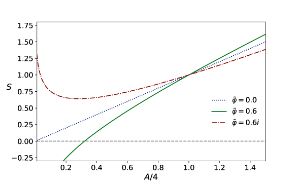
Figure 1: Entropy curves for Bekenstein-Hawking ($\tilde{\varphi}=\varphi=0$), and vector Galileon with real and imaginary $\varphi$. For imaginary $\tilde{\varphi}$ (imaginary $Q$) there is a region where the entropy decreases as the area increases, while for real $\tilde{\varphi}$ (real $Q$) there is region with negative entropy.

In Fig. 1 we illustrate the properties mentioned above.

The possibility of considering real and imaginary $\varphi$ (or equivalently $Q$) arises from the following observation: taking the equations of motion of the vector galileons for the spherically symmetric ansatz, Eqs. (3), together with the vector field solutions  (5,6) and with the condition $P\propto Q$ imposed when obtaining the entropy, we see that if $Q$ is allowed to be imaginary, then $P$ also becomes imaginary, and as a consequence $A_{0}(r)$ and $\pi(r)$ are pure imaginary numbers, which implies that the energy-momentum tensor of the vector field remains real, since it depends quadratically on $A_{0}(r),\pi(r)$. Therefore, it is consistent to consider an imaginary $Q$. In the next section we explore other consequences of the VG modified entropy, arising in the context of entropic gravity.

IV Phenomenology

In this section we explore two possible phenomenological signatures of the black hole entropy derived above. In the first part, we study implications for the area law, which has been supported observationally in [27]. In the second part, we explore consequences that arise in the context of entropic gravity.

IV.1 Area law

In 1971 [26] Hawking derived an important theorem in GR that shows that the surface area of a classical black hole can never decrease. This applies also if two black holes merge into a single one: the surface area of the final black hole must be strictly greater than the sum of the areas of the original black holes. It is important to highlight the the area theorem is not in general valid in modified gravity [37]. Hawking’s area theorem is also known as the second law of black hole mechanics, and establishes an analogy to the second law of thermodynamics and the entropy. The idea of testing this theorem with observations of gravitational waves has been discussed in Refs. [38, 39, 40], and recently in Ref. [27] it was applied to actual LIGO-Virgo data from GW150914 [41]. The recent possibilities for observational verification of the area theorem makes it relevant to also investigate theoretical aspects in the relation between area and entropy. While for the Bekenstein-Hawking entropy, $S_{BH}=\frac{A}{4}$, it is true that an increment of the area leads to an increment of the entropy, this is not always the case for a modified entropy, such as Eq. (56). For instance, consider two black holes of the same area $A_{1}$, that merge into a black hole with a certain final area $A_{f}$. Since the charge $Q$ is not a property of the black hole, we assume that the initial and final entropies are modified by the same factor of $Q$. Let us focus on the entropy for imaginary $Q$, Eq. (58), which seems to be more in tension with the area theorem, as it allows for a reduction in area alongside a positive change in entropy. Thus, for Eq. (58), the total initial entropy is

$$S_{i} =\frac{{A_{1}}}{4}+\frac{{A_{1}}}{4}-\frac{1}{4}\pi{\varphi}^{2}\ln\left(\frac{{A_{1}}}{4}\right)-\frac{1}{4}\pi{\varphi}^{2}\ln\left(\frac{{A_{1}}}{4}\right)$$

$$=\frac{A_{i}}{4}-\frac{1}{2}\pi\varphi^{2}\ln\left(\frac{A_{i}}{8}\right),$$ (59)

and the final entropy is

$$S_{f}=\frac{A_{f}}{4}-\frac{1}{4}\pi\varphi^{2}\ln\frac{A_{f}}{4},$$ (60)

where $A_{i}=2A_{1}$. Defining $A_{f}/A_{i}=\sigma$ ($\sigma>1$ when the area theorem holds) the change in entropy is

$$\Delta S\equiv S_{f}-S_{i}=\frac{1}{4}\left((\sigma-1)A_{i}-\pi\varphi^{2}\ln\left(\frac{16\sigma}{A_{i}}\right)\right).$$ (61)

Assuming $\sigma>1$ the first term is always positive. However, the second term can push $\Delta S$ to negative values, i.e., the fact that the area grows is not enough to guarantee that the change in entropy is positive. In the left panel of Fig. 2 we represent $\Delta S$ as a function of the total area of the initial configuration, $A_{i}$, and the ratio $A_{f}/A_{i}=\sigma>1$. The charge is fixed at $\varphi=1.2$. The black solid line is the level curve $\Delta S=0$, below this line the change in entropy is negative. The middle panel of Fig. 2 shows the level curves $\Delta S=0$ for different values of $\varphi$. For each $\varphi$, the change in entropy is similar to the one displayed in the left panel. An important observation, either from Eq. (61) or from Fig. 2, is that for any initial area $A_{i}>16$ and $\varphi<2\sqrt{{e}/\pi}$, it is true that an increase in area leads to an increase in entropy. For smaller $A_{i}$ the situation is different, for instance, if $A_{i}\sim 5$, a positive increment of the entropy requires that the final area is around $A_{f}\sim 1.2A_{i}$. Thus, the area theorem $A_{f}>A_{i}$ is not enough to guarantee a never decreasing black hole entropy, instead, a stronger bound $A_{f}>m(\varphi,A_{i})A_{i}$, with $m(\varphi,A_{i})>1$ a function of $\varphi$ and $A_{i}$ and $m(\varphi,A_{i}=16)=1$, is required. The right panel of Fig. 2 shows that a positive change in entropy is also possible when the final area is smaller than the initial area. Finally, it is important to highlight that these details in the relation between area and entropy would be observable only for Planck scale black holes, as can be determined by translating $A_{i}>16$ to physical units.

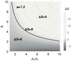
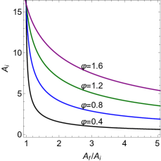
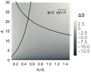
Figure 2: Left: regions where an increment of area leads to a negative ($\Delta S<0$) or positive ($\Delta S>0$) change in entropy. The solid line is the curve $\Delta S=0$. Middle: Curves $\Delta S=0$ for different values of the charge $\varphi$. Right: Processes where $A_{f}<A_{i}$ are possible even with a positive change in entropy, which corresponds to the left and top right regions of the plot.

IV.2 Entropic Gravity

The notion of gravity as an emergent phenomenon was put forward by Jacobson [42] by noting that the Einstein field equations can be viewed as a thermodynamic equation of state when considering that the Clausius relation $\delta E=TdS$ between heat, temperature and entropy holds for every local Rindler horizon (heat is usually denoted by $Q$ in the literature; we use $E$ to avoid confusion with the vector charge $Q$). In the spirit of Jacobson’s work and in analogy to emergent entropic forces in polymers [43], Verlinde [28] proposed that gravity is an effective force which emerges from the entropy via $F\Delta x=T\Delta S$. Building on these ideas and motivated by aspects of Loop Quantum Gravity, Modesto and Randono [29] modified Verlinde’s assumptions, in particular on the construction of $\Delta S$, arriving at the following conclusion: given a test mass $m$ at a distance $R$ of a source of mass $M$, when a change on the entropy of a surface $\mathcal{S}$ of radio $R$ occurs, there appears a force due to that change, given by

$$\mathbf{F}=-\left.\frac{GMm}{R^{2}}4\ell_{P}^{2}\frac{\partial S}{\partial A}\right|_{A=4\pi R^{2}}\mathbf{\hat{R}},$$ (62)

where $\ell_{P}$ is Planck length. If one assumes the horizon entropy to be given by the Bekenstein-Hawking formula, $S_{BH}=A/4\ell_{P}^{2}$, then Eq. (62) yields the Newtonian force. However, it is of interest to consider different entropies. One of the most studied modifications is the well-known logarithmic correction, which has been suggested to be a universal correction term for the Bekeinstein-Hawking entropy,

$$S(A)=\frac{A}{4\ell_{P}^{2}}-\alpha\ln\frac{A}{4\ell_{P}^{2}},$$ (63)

with $\alpha$ a dimensionless parameter. For this correction term, the modified Newtonian force and the corresponding potential function have been obtained [44]. Comparing with the entropy-area relation (58) for vector Galileons obtained in Sec. III, we identify

$$\varphi=2\sqrt{\frac{\alpha}{\pi}}.$$ (64)

The modified force associated to this entropy is

$$\mathbf{F}=-\frac{GMm}{R^{2}}\left[1-\left(\frac{l_{p}\varphi}{2R}\right)^{2}\right]\mathbf{\hat{R}}.$$ (65)

It is worth clarifying the following: evidently, from the Schwarzschild metric and the equivalence principle, both in GR and vector Galileons we could deduce that in the weak field limit the trajectory of a particle is determined by the metric, and therefore by the Newtonian potential $\sim 1/r$ without any corrections. For vector Galileons, this seems incompatible with the corrected force that arises in the entropic formalism. However, we must emphasise that the correction to the Newtonian potential derived from the logarithmic entropy is identified as a perturbative quantum gravity effect [29] (notice that this correction is weighted by the square of the Planck length). Therefore, we do not expect to obtain this correction from a classical weak field analysis. The potential function associated to (65) is

$$\Phi=-\frac{GM}{R}\left[1-\frac{1}{3}\left(\frac{\ell_{P}\varphi}{2R}\right)^{2}\right].$$ (66)

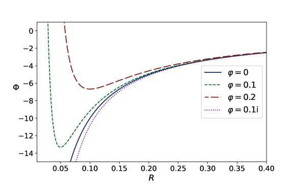
Figure 3: Plot of the potential function Eq. (66) for different values of the parameter $\varphi$. When $\varphi\in\mathbb{R}$ and $\varphi\neq 0$ (imaginary $Q$), the potential develops a minimum, while for imaginary values (real $Q$) it behaves qualitatively like the ordinary Newtonian potential.

As discussed before, the theory admits both real and imaginary $Q$ (and therefore $\varphi$), and this determines the relative sign between the terms of the modified potential (66). A plot of the modified potential for different values of $\varphi$ is shown in Fig. 3. Quantitative effects of these (and other) modifications have been studied in the context of planetary orbits [45]. Comparing to their results and using Eq. (64) we see, for instance, that the correction to Mercury’s precession weighted by $\varphi^{2}$ is around $10^{84}$ times smaller than the observational result. Thus, extremely large vector charges would be needed to get a relevant contribution from the logarithmic correction. For modified forces and potentials obtained from an entropy-area relation with further correction terms, see [46].

The ideas of Jacobson have also been applied in cosmological scenarios [30, 47, 32]. In [30], this is done by considering the Clausius relation on the apparent horizon of a Friedmann-Robertson-Walker (FRW) universe and assigning a given temperature and entropy to the horizon. The energy flow on the apparent horizon is determined by the matter content, which is considered to be a perfect fluid. If one assumes the horizon entropy to be given by the Bekenstein-Hawking formula, then the Clausius relation together with the continuity equation yield the Friedmann equation for the FRW universe. On the other hand, if one considers a modified entropy-area relationship on the horizon, then a modified Friedmann equation is obtained. In [30] the following modified Friedmann equation for a flat universe arising in the context of quantum cosmology is considered,

$$H^{2}=\frac{8\pi G}{3}\rho\left(1-\frac{\rho}{\rho_{\mathrm{crit}}}\right).$$ (67)

Due to the modification term in this equation, the big bang singularity is replaced by a quantum bounce happening at $\rho=\rho_{\mathrm{crit}}$. The modified Friedmann Eq. (67) can be obtained from the modified entropy-area relation

$$S=\frac{A}{4\ell_{P}^{2}}+\frac{3}{4\pi G^{2}\rho_{\text{crit }}}{\frac{c^{5}}{\hbar}}\ln\frac{A}{4\ell_{P}^{2}},$$ (68)

where $A$ is the area of the horizon. Although this form of the entropy is the familiar one with the logarithmic correction, in this case the correction term gives an opposite contribution to the entropy, since the prefactor in the logarithmic term is positive. We see that this entropy is equivalent to (56) with the identification of a real $\varphi$,

$$\tilde{\varphi}^{2}=\frac{4}{\pi}\left(\frac{3}{4\pi G^{2}\rho_{\text{crit }}}{\frac{c^{5}}{\hbar}}\right).$$ (69)

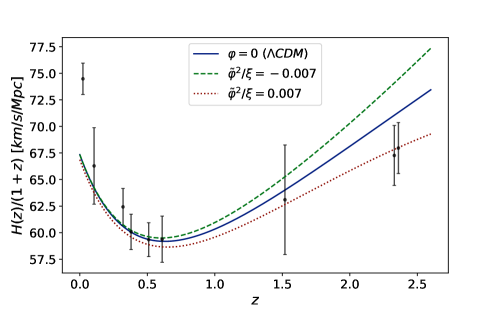
Figure 4: Plot of $H(z)/(1+z)$ for the modified Friedmann Eq. (71) that comes from the entropy (56) (dotted). We also plot the case that corresponds to the entropy (58) (dashed). Points and errors bars are taken from observational Hubble data compiled in [48].

In order to study some consequences of the modified Friedmann Eq. (67), let us express the density as $\rho=\rho_{M}+\rho_{\Lambda}$, where $\rho_{M}$ stands for non relativistic matter $\rho_{M}(z)=\rho_{0M}(1+z)^{3}$, and $\rho_{\Lambda}$ for the constant dark energy density $\rho_{\Lambda}=\Lambda/8\pi G$, and let us introduce the density parameters at present time,

$$\Omega_{0M}=\frac{8\pi G\rho_{0M}}{3H_{0}^{2}},\quad\Omega_{0\Lambda}=\frac{\Lambda}{3H_{0}^{2}}.$$ (70)

With this, we can rewrite Eq. (67) as

$$\frac{H(z)^{2}}{H_{0}^{2}}= \Omega_{0M}(1+z)^{3}+\Omega_{0\Lambda}\left(1-\frac{\tilde{\varphi}^{2}}{\xi}\Omega_{0\Lambda}\right)-2\frac{\tilde{\varphi}^{2}}{\xi}\Omega_{0M}\left[\Omega_{0\Lambda}+\frac{\Omega_{0M}}{2}(1+z)^{3}\right](1+z)^{3},$$ (71)

where we have defined the dimensionless parameter

$$\xi=\frac{8}{\pi GH_{0}^{2}}{\frac{c^{5}}{\hbar}}.$$ (72)

Note that in the limit $\tilde{\varphi}\to 0$ the usual Friedmann equation is recovered. In figure 4 we show a plot of $H(z)/(1+z)$ for different values of $\tilde{\varphi}^{2}/\xi$. We see that the modifications to the Hubble factor are larger for large redshift, and depending on whether $Q$ is real ($\tilde{\varphi}\in\mathbb{R}$) or imaginary ($\varphi\in\mathbb{R}$), the values of $H(z)$ are smaller or larger, respectively, than in $\Lambda$CDM. The values of $\tilde{\varphi}$ used for this figure are exaggerated in order to make their effect noticeable. Since $\xi\sim 10^{122}$, extremely large values for $\tilde{\varphi}$ would be needed in order to obtain relevant modifications to the evolution of the Hubble factor.

V Conclusions

We studied the entropy of a Schwarzschild black hole dressed with a non-trivial vector field in a model belonging to generalised Proca theories, also known as vector Galileons. The non-trivial vector field has both a temporal and a radial component, whose profiles depend on two integration constants. In principle, these integration constants are independent; however, consistency with the first law of black hole mechanics demands a relation between these constants and the black hole mass, leaving only two independent quantities that can be identified as charges of the black hole and vector field. The fact that some conditions need to be imposed on the parameters of the solutions of vector Galileon theories had been pointed out in [25, 36], but a complete calculation had not been performed so far.

After imposing the appropriate constraints, we find that the entropy matches the Bekenstein-Hawking relation with a logarithmic contribution modulated by the independent charge of the vector field. This is relevant because logarithmic corrections to the entropy are considered to be universal. A logarithmic term in the entropy is usually associated to quantum corrections, whose back-reaction on the black hole geometry needs to be taken into account in order to get a fully consistent analysis. However, in our results the logarithmic correction arises from a classical action and an exactly Schwarzschild background, signalling the existence of particular cases where additional fields of the theory protect the metric from the back-reaction expected from logarithmic corrections. It would be interesting to explore this idea in the context of effective field theories that have been recently applied to obtain the back-reaction on the metric [49, 50].

We analysed some consequences of the logarithmic contribution to the entropy. Since our calculation is classical, in principle the logarithmic part of the entropy does not need to be treated as a small correction term. Demanding that the entropy is always increasing, we find an upper bound on the vector charge, of the form $-Q^{2}\lesssim{A}$ (in the case where $Q$ is pure imaginary). This still allows for the possibility of large vector charges in large black holes, raising the question of whether this modified entropy could be verified experimentally. An interesting direction along these lines is the observational corroboration of the area theorem of GR, which exploits the fact that a consequence of this theorem is that when two black holes merge into a single one, the area of the final black hole is larger than the sum of the areas of the initial configurations. In modified gravity, the area theorem is not in general valid. Assuming that the entropy is the quantity that needs to be always increasing, we find that the condition on the area can be relaxed. i.e., a decreasing area can be compatible with an increasing modified entropy. Thus, an observation of a decreasing area would be problematic for GR, but not for theories with logarithmic corrections to the entropy. However, our results indicate that this is only an issue for Planck scale black holes. At these scales, we expect quantum corrections to modify our predictions.

In addition, following the arguments of entropic gravity, the logarithmic correction to the entropy translates into a modified Newtonian potential, which has consequences, e.g. for planetary orbits [45]. Finally, also in the context of entropic gravity, we review the modified Friedmann equations resulting from the logarithmic correction to the entropy, and we use there results to analyse cosmological effects of the vector charge. Both in the astrophysical and cosmological scenarios, we find that the corrections due to the vector charge are several orders of magnitude smaller than the classical scales of the respective problems.

References

- [1] P. A. R. Ade et al. Planck 2015 results. XIII. Cosmological parameters. Astron. Astrophys., 594:A13, 2016.
- [2] Kazunori Akiyama et al. First M87 Event Horizon Telescope Results. I. The Shadow of the Supermassive Black Hole. Astrophys. J. Lett., 875:L1, 2019.
- [3] B. P. Abbott et al. Tests of General Relativity with the Binary Black Hole Signals from the LIGO-Virgo Catalog GWTC-1. Phys. Rev. D, 100(10):104036, 2019.
- [4] R. Abbott et al. Tests of general relativity with binary black holes from the second LIGO-Virgo gravitational-wave transient catalog. Phys. Rev. D, 103(12):122002, 2021.
- [5] Kazunori Akiyama et al. First Sagittarius A* Event Horizon Telescope Results. I. The Shadow of the Supermassive Black Hole in the Center of the Milky Way. Astrophys. J. Lett., 930(2):L12, 2022.
- [6] Eugeny Babichev and Christos Charmousis. Dressing a black hole with a time-dependent Galileon. JHEP, 08:106, 2014.
- [7] Tsutomu Kobayashi and Norihiro Tanahashi. Exact black hole solutions in shift symmetric scalar–tensor theories. PTEP, 2014:073E02, 2014.
- [8] Adolfo Cisterna, Mokhtar Hassaine, Julio Oliva, and Massimiliano Rinaldi. Static and rotating solutions for Vector-Galileon theories. Phys. Rev. D, 94(10):104039, 2016.
- [9] Masato Minamitsuji. Solutions in the generalized Proca theory with the nonminimal coupling to the Einstein tensor. Phys. Rev. D, 94(8):084039, 2016.
- [10] Javier Chagoya, Gustavo Niz, and Gianmassimo Tasinato. Black Holes and Abelian Symmetry Breaking. Class. Quant. Grav., 33(17):175007, 2016.
- [11] Eugeny Babichev, Christos Charmousis, and Antoine Lehébel. Asymptotically flat black holes in Horndeski theory and beyond. JCAP, 04:027, 2017.
- [12] Jibril Ben Achour and Hongguang Liu. Hairy Schwarzschild-(A)dS black hole solutions in degenerate higher order scalar-tensor theories beyond shift symmetry. Phys. Rev. D, 99(6):064042, 2019.
- [13] Masato Minamitsuji and James Edholm. Black hole solutions in shift-symmetric degenerate higher-order scalar-tensor theories. Phys. Rev. D, 100(4):044053, 2019.
- [14] Hayato Motohashi and Masato Minamitsuji. Exact black hole solutions in shift-symmetric quadratic degenerate higher-order scalar-tensor theories. Phys. Rev. D, 99(6):064040, 2019.
- [15] Kazufumi Takahashi and Hayato Motohashi. General Relativity solutions with stealth scalar hair in quadratic higher-order scalar-tensor theories. JCAP, 06:034, 2020.
- [16] Claudia de Rham and Jun Zhang. Perturbations of stealth black holes in degenerate higher-order scalar-tensor theories. Phys. Rev. D, 100(12):124023, 2019.
- [17] Antonio De Felice, Shinji Mukohyama, and Kazufumi Takahashi. Approximately stealth black hole in higher-order scalar-tensor theories. JCAP, 03:050, 2023.
- [18] Lavinia Heisenberg. Generalization of the Proca Action. JCAP, 05:015, 2014.
- [19] Gianmassimo Tasinato. Cosmic Acceleration from Abelian Symmetry Breaking. JHEP, 04:067, 2014.
- [20] Zhong-Ying Fan. Black holes with vector hair. JHEP, 09:039, 2016.
- [21] Javier Chagoya, Gustavo Niz, and Gianmassimo Tasinato. Black Holes and Neutron Stars in Vector Galileons. Class. Quant. Grav., 34(16):165002, 2017.
- [22] Eugeny Babichev, Christos Charmousis, and Mokhtar Hassaine. Black holes and solitons in an extended Proca theory. JHEP, 05:114, 2017.
- [23] Lavinia Heisenberg, Ryotaro Kase, Masato Minamitsuji, and Shinji Tsujikawa. Hairy black-hole solutions in generalized Proca theories. Phys. Rev. D, 96(8):084049, 2017.
- [24] Lavinia Heisenberg, Ryotaro Kase, Masato Minamitsuji, and Shinji Tsujikawa. Black holes in vector-tensor theories. JCAP, 08:024, 2017.
- [25] Zhong-Ying Fan. Black holes in vector-tensor theories and their thermodynamics. Eur. Phys. J. C, 78(1):65, 2018.
- [26] S. W. Hawking. Black holes in general relativity. Commun. Math. Phys., 25:152–166, 1972.
- [27] Maximiliano Isi, Will M. Farr, Matthew Giesler, Mark A. Scheel, and Saul A. Teukolsky. Testing the black-hole area law with gw150914. Phys. Rev. Lett., 127:011103, Jul 2021.
- [28] Erik P. Verlinde. On the Origin of Gravity and the Laws of Newton. JHEP, 04:029, 2011.
- [29] Leonardo Modesto and Andrew Randono. Entropic Corrections to Newton’s Law. 3 2010.
- [30] Rong-Gen Cai, Li-Ming Cao, and Ya-Peng Hu. Corrected Entropy-Area Relation and Modified Friedmann Equations. JHEP, 08:090, 2008.
- [31] Ahmad Sheykhi and Seyed Hossein Hendi. Power-Law Entropic Corrections to Newton’s Law and Friedmann Equations. Phys. Rev. D, 84:044023, 2011.
- [32] Ahmad Sheykhi. Thermodynamics of apparent horizon and modified Friedmann equations. Eur. Phys. J. C, 69:265–269, 2010.
- [33] Robert M. Wald. Black hole entropy is the Noether charge. Phys. Rev. D, 48(8):R3427–R3431, 1993.
- [34] Vivek Iyer and Robert M. Wald. Some properties of Noether charge and a proposal for dynamical black hole entropy. Phys. Rev. D, 50:846–864, 1994.
- [35] Xing-Hui Feng, Hai-Shan Liu, H. Lü, and C. N. Pope. Black Hole Entropy and Viscosity Bound in Horndeski Gravity. JHEP, 11:176, 2015.
- [36] Ai-chen Li. Counterterm method and thermodynamics of hairy black holes in a vector-tensor theory with Abelian gauge symmetry breaking. Phys. Rev. D, 104(4):044040, 2021.
- [37] Sudipta Sarkar. Area Theorem: General Relativity and Beyond. Fundam. Theor. Phys., 187:363–374, 2017.
- [38] Scott A. Hughes and Kristen Menou. Golden binaries for LISA: Robust probes of strong-field gravity. Astrophys. J., 623:689–699, 2005.
- [39] Gian F. Giudice, Matthew McCullough, and Alfredo Urbano. Hunting for Dark Particles with Gravitational Waves. JCAP, 10:001, 2016.
- [40] Miriam Cabero, Collin D. Capano, Ofek Fischer-Birnholtz, Badri Krishnan, Alex B. Nielsen, Alexander H. Nitz, and Christopher M. Biwer. Observational tests of the black hole area increase law. Phys. Rev. D, 97:124069, Jun 2018.
- [41] B. P. Abbott et al. Observation of Gravitational Waves from a Binary Black Hole Merger. Phys. Rev. Lett., 116(6):061102, 2016.
- [42] Ted Jacobson. Thermodynamics of space-time: The Einstein equation of state. Phys. Rev. Lett., 75:1260–1263, 1995.
- [43] Igor M Sokolov. Statistical mechanics of entropic forces: disassembling a toy. European journal of physics, 31(6):1353, 2010.
- [44] Aldo Martínez-Merino, Octavio Obregón, and Michael P. Ryan, Jr. Modified entropies, their corresponding Newtonian forces, potentials, and temperatures. Phys. Rev. D, 95(12):124031, 2017.
- [45] G. Pérez-Cuéllar and M. Sabido. On planetary orbits in entropic gravity. Mod. Phys. Lett. A, 36(08):08, 2021.
- [46] I. Díaz-Saldaña, J. C. López-Domínguez, and M. Sabido. On Emergent Gravity, Black Hole Entropy and Galactic Rotation Curves. Phys. Dark Univ., 22:147–151, 2018.
- [47] I. Díaz-Saldaña, J. López-Domínguez, and M. Sabido. An Effective Cosmological Constant From an Entropic Formulation of Gravity. Int. J. Mod. Phys. D, 29(09):2050064, 2020.
- [48] Hai Yu, Bharat Ratra, and Fa-Yin Wang. Hubble Parameter and Baryon Acoustic Oscillation Measurement Constraints on the Hubble Constant, the Deviation from the Spatially Flat CDM Model, the Deceleration–Acceleration Transition Redshift, and Spatial Curvature. Astrophys. J., 856(1):3, 2018.
- [49] Yong Xiao and Yu Tian. Logarithmic correction to black hole entropy from the nonlocality of quantum gravity. Phys. Rev. D, 105(4):044013, 2022.
- [50] Xavier Calmet and Folkert Kuipers. Quantum gravitational corrections to the entropy of a Schwarzschild black hole. Phys. Rev. D, 104(6):066012, 2021.