Efficient Full-frequency GW Calculations using a Lanczos Method

Abstract

The GW approximation is widely used for reliable and accurate modeling of single-particle excitations. It also serves as a starting point for many theoretical methods, such as its use in the Bethe-Salpeter equation (BSE) and dynamical mean-field theory. However, full-frequency GW calculations for large systems with hundreds of atoms remain computationally challenging for most researchers, even after years of efforts to reduce the prefactor and improve scaling. We propose a method that reformulates the correlation part of GW self-energy as a resolvent of a Hermitian matrix, which can be efficiently and accurately computed using the Lanczos method. This method enables GW calculations of material systems with a few hundred atoms on a single computing workstation. We further demonstrate the efficiency of the method by calculating the defect-state energies of silicon quantum dots with diameters up to 4 nm and nearly 2,000 silicon atoms using only 20 compute nodes.

As a first-principles approach based on many-body perturbation theory, the GW approximation has been successfully applied to accurately compute quasiparticle excitation in weakly and moderately correlated materials [1, 2, 3]. The approximation also plays an essential role in the first-principles calculations of excitonic effects using the GW+BSE approach [4, 5] and is used in conjunction with other methods [6, 7, 8, 9, 10, 11]. The computational costs of common implementations of GW approximation typically scale as $O(N^{3})$ to $O(N^{6})$ and have larger pre-factors compared to density functional theory (DFT) calculations with semi-local exchange-correlation functionals [12].

During the last decade, different formulations and algorithms have been proposed and implemented for accelerating GW calculations to meet the challenge of modeling large and complex materials [12, 13]. A few seminal papers have demonstrated GW calculations of quasiparticle energies of large systems with the number of atoms ranging from 1,000 to around 2,700 [14, 15, 16, 17, 18]. These large-scale GW calculations rely on well-crafted numerical optimization and large computation resources, which are of limited accessibility. Even with notable advancements, GW calculations for systems with a few hundred atoms, which are typically required for computationally studying a point defect in solids or small quantum dots, cannot be performed routinely. Owing to the significant expense of data curation, GW calculations are rarely used in wide-reaching data-driven research, such as constructing large databases of material properties and training supervised machine-learning models.

In GW calculations, the computationally limiting step is evaluating the frequency-dependent screened Coulomb potential. In many implementations, the irreducible polarizability function and then the inverse dielectric function are calculated to compute $W$ [19, 20]. Such a procedure deals with the frequency dependence of $W$ using approximations like plasmon-pole models or numerical tools such as contour deformation or analytical continuations [12, 21]. Alternatively, another approach computes the reducible polarizability and $W$ by solving the Casida equation derived in linear-response time-dependent density functional theory [22, 23, 24, 25, 26]. Once all the eigenvalues and eigenvectors of the Caisda equation are solved, the frequency-dependent $W$ and GW quasiparticle self-energies can be written and computed in a closed form [23, 24, 25]. While this approach is formally simple and works efficiently for small systems with less than 50 atoms, it becomes numerically intractable for large systems due to the high cost of solving the Casida equation.

Here, we propose a method that avoids solving the Casida equation while still allowing us to perform full-frequency GW calculations analytically and efficiently. To better illustrate the concept, we discuss our method applied to finite systems, for which real-valued wave functions and simplified notations can be used. Initially, we perform DFT calculations to obtain Kohn-Sham orbitals $|\phi_{m}\rangle$ and their corresponding energies $\epsilon_{m}$, which are used as an initial approximation for quasiparticle wave functions and energies, respectively. Next, the Casida equation can be constructed [22, 24, 23, 27]

$$\begin{pmatrix}\mathbf{A}&\mathbf{B}\\ -\mathbf{B}&-\mathbf{A}\end{pmatrix}\begin{pmatrix}X^{s}\\ Y^{s}\end{pmatrix}=\begin{pmatrix}X^{s}\\ Y^{s}\end{pmatrix}\Omega_{s},$$ (1)

The dimension of matrices $\mathbf{A}$ and $\mathbf{B}$ is $N_{vc}^{2}$, where $N_{vc}=N_{v}\cdot N_{c}$ scales as $O(N^{2})$ with respect to system size $N$. Here $N_{v}$ and $N_{c}$ represent the number of occupied and empty orbitals, respectively. With the random-phase approximation (RPA) used in the GW approximation, the matrix elements of $\mathbf{A}$ and $\mathbf{B}$ are given as

$$\mathbf{A}_{vc,v^{\prime}c^{\prime}} = (\epsilon_{c}-\epsilon_{v})\delta_{vv^{\prime}}\delta_{cc^{\prime}}+(vc|v^{\prime}c^{\prime})$$ (2)

$$\mathbf{B}_{vc,v^{\prime}c^{\prime}} = (vc|c^{\prime}v^{\prime})$$ (3)

$$= \int\int\frac{\phi_{v}(\mathbf{r})\phi_{c}(\mathbf{r})\phi_{c^{\prime}}(\mathbf{r}^{\prime})\phi_{v^{\prime}}(\mathbf{r}^{\prime})}{|\mathbf{r}-\mathbf{r}^{\prime}|}d^{3}rd^{3}r^{\prime}$$

We use indices $v$ and $v^{\prime}$ for occupied states, $c$ and $c^{\prime}$ for empty states, and $k$, $l$, $n$, and $m$ for general orbitals, respectively. For finite systems, the Casida equation can be reformulated as a smaller eigenvalue problem [23, 24]

$$\mathbf{C}Z^{s} = Z^{s}\Omega^{2}_{s}$$ (4)

where $\mathbf{C}=(\mathbf{A}-\mathbf{B})^{1/2}(\mathbf{A}+\mathbf{B})(\mathbf{A}-\mathbf{B})^{1/2}$ is a symmetric matrix of dimension $N^{2}_{vc}$. After solving Eq. 4 for the eigenpairs $(Z^{s},\Omega^{2}_{s})$ of $\mathbf{C}$, one can compute the GW self-energy

$$\langle\phi_{m}|\Sigma^{\mathbf{GW}}(\omega)|\phi_{m}\rangle=\Sigma^{\mathrm{ex}}_{mm}+\Sigma^{\mathrm{corr}}_{mm}(\omega),$$ (5)

$$\Sigma^{\mathrm{ex}}_{mm}=-\sum_{v}(vm|vm),$$ (6)

$$\Sigma^{\mathrm{corr}}_{mm}(\omega)=\sum^{N_{v}+N_{c}}_{n}\sum^{N_{vc}}_{s}\frac{W^{s}_{nm}W,^{s}_{nm}}{\omega-\epsilon_{n}+\eta_{n}(\Omega_{s}-i\delta)}$$ (7)

where $\eta_{n}$ is 1 for occupied orbitals and -1 for empty orbitals, and $\delta$ is a positive infinitesimal number to avoid singularity. The matrix elements $W^{s}_{nm}$ are

$$W^{s}_{nm} = \sum_{vc}(nm|vc)\sqrt{\frac{\epsilon_{c}-\epsilon_{v}}{\Omega_{s}}}Z^{s}_{vc}.$$ (8)

The exchange part of the self-energy $\Sigma^{\mathrm{ex}}_{mm}$ is independent of frequency and relatively easy to compute, while the correlation part $\Sigma^{\mathbf{corr}}_{mm}(\omega)$ includes the frequency-dependent screening effects of dielectric responses. The poles of frequency-dependent screened effects can be determined by the eigenvalues of $\mathbf{C}$. As a result, the most expensive step of the aforementioned method is diagonalizing the Casida equation, as the computational cost scales as $O(N^{6})$. To make further progress, we intend to avoid this costly step by defining a vector $|P_{nm}\rangle$ of dimension $N_{vc}$, which has elements given by $(P_{nm})_{vc}=(nm|vc)(\epsilon_{c}-\epsilon_{v})^{1/2}$. Then $W^{s}_{nm}$ reads

$$W^{s}_{nm} = \langle P_{nm}|Z^{s}\rangle\Omega_{s}^{-\frac{1}{2}}.$$ (9)

$\Sigma^{\mathrm{corr}}_{mm}$ can be rewritten as

$$\Sigma^{\mathrm{corr}}_{mm}(\omega) = \sum^{N_{v}+N_{c}}_{n=1}\Sigma^{\mathrm{corr}}_{mm}(\omega,n),$$ (10)

where

$$\Sigma^{\mathrm{corr}}_{mm}(\omega,n) = \frac{1}{z_{n}}\sum^{N_{vc}}_{s=1}\langle P_{nm}|Z^{s}\rangle\langle Z^{s}|P_{nm}\rangle\times$$ (11)

$$\Big{[}\frac{1}{\Omega_{s}}-\frac{1}{\Omega_{s}+\eta_{n}z_{n}}\Big{]},$$

where $z_{n}=\omega-\epsilon_{n}-i\eta_{n}\delta$.

Examining Eq. 11, we note the formula for $\Sigma^{\mathrm{corr}}_{mm}(\omega,n)$ is similar to a general resolvent matrix element of the form $\sum_{k}\langle\star|k\rangle\langle k|\star\rangle/(z-\lambda_{k})=\langle\star|1/(z-\mathbf{H})|\star\rangle$, where $\mathbf{H}$ is a general Hermitian matrix with eigenvalues $\lambda_{k}$ and eigenvectors $|k\rangle$, $z$ is a complex number, and $|\star\rangle$ is a ket. Motivated by this observation, we reformulate Eq. 11 as the resolvent of a symmetric matrix $\mathbf{D}$

$$\Sigma^{\mathrm{corr}}_{mm}(\omega,n) = \frac{1}{z_{n}}\langle P_{nm}|\frac{1}{\mathbf{D}}-\frac{1}{\mathbf{D}+\eta_{n}z_{n}}|P_{nm}\rangle.$$ (12)

Matrix $\mathbf{D}$ satisfies $\mathbf{D}^{2}=\mathbf{C}$ and its eigenvalues are the square root of those of matrix C, i.e., $\mathbf{D}Z^{s}=Z^{s}\Omega_{s}$. We use a $g$-th degree polynomial function $p_{g}$ to fit the square root function $p_{g}(x)=\sum^{g}_{k=0}a_{k}x^{k}\approx\sqrt{x}$ within the range between minimum and maximum eigenvalues of matrix $\mathbf{C}$. Accordingly, $\mathbf{D}$ can be approximated by $\mathbf{D}=p_{g}(\mathbf{C})+\Delta_{g}\approx p_{g}(\mathbf{C})=a_{0}\mathbf{I}+\sum^{g}_{k=1}a_{k}\mathbf{C}^{k}$, where $\mathbf{I}$ is an identity matrix and the fitting error $\Delta_{g}$ can be controlled via the degree $g$ of the polynomial function and fitting procedures.

Given Eq. 12 and matrix $\mathbf{D}$, the Lanczos method can then be applied to efficiently compute the resolvent of matrix $\mathbf{D}$, which is an important step of calculating $\Sigma^{\mathrm{corr}}_{mm}(\omega,n)$. In the calculation of $\Sigma^{\mathrm{corr}}_{mm}(\omega)$, we prepare $|P_{nm}\rangle$ for each state $n$ in the summation of Eq. 10, where $|P_{nm}\rangle$ is used as the starting vector for the Lanczos tri-diagonalization procedure of the symmetric matrix $\mathbf{D}$. With $L$ steps of Lanczos iterations, one can construct a tridiagonal matrix $\mathbf{D}_{L}$ with dimension $L$ in the following form

$$\mathbf{D}_{L}=\begin{pmatrix}a_{0}&b_{1}&0&\ldots&0&0\\ b_{1}&a_{1}&b_{2}&\ldots&0&0\\ 0&b_{2}&a_{2}&\ldots&0&0\\ \vdots&\vdots&\vdots&\ddots&\vdots&\vdots\\ 0&0&0&\ldots&a_{L-1}&b_{L}\\ 0&0&0&\ldots&b_{L}&a_{L}\end{pmatrix}.$$ (13)

Once the tridiagonal matrix $\mathbf{D}_{L}$ is obtained, a resolvent matrix element (such as Eq. 12) can be computed using the continuous fraction

$$\langle P_{nm}|\frac{1}{z-\mathbf{D}}|P_{nm}\rangle=\frac{1}{z-a_{0}-\frac{b^{2}_{1}}{z-a_{1}-\frac{b^{2}_{2}}{a_{2}-\ldots}}},$$ (14)

which is also known as the Haydock method [28]. The computation of Eq. 14 is efficient, and one can easily calculate the quasiparticle energies for a series of frequencies by varying $z$ in Eq. 14. When applied to eigenvalue problems, the Lanczos algorithm can lead to ghost eigenvalues. However, applying the Lanczos method to calculate resolvent is free of the numerical problem [29].

There are several advantages of using a Lanczos method for computing $\Sigma^{\mathrm{corr}}_{mm}$. Solving the eigenvalue problem given by the Casida equation is avoided and the resulting GW calculations become more efficient than the conventional method represented by Eq. 7, which explicitly requires the eigenpairs of the Casida equation. Frequency grids, analytical continuation, and approximations like plasmon-pole models are not required, as the frequency dependence of $W$ and $\Sigma^{\mathrm{corr}}_{mm}$ are implicitly treated via Lanczos iterations. Moreover, our method is in principle applicable to any basis sets of wave functions, as our derivation does not rely on any features of specific basis functions.

As a general-purpose algorithm, Lanczos-based methods have been used in computational material science, such as computing Green’s function [28], optical absorption spectra with linear-response time-dependent density functional theory [30, 31, 32, 33, 34] and Bethe-Salpeter equation [35]. Earlier work [36, 37, 38] applied Lanczos methods for solving the Sternheimer equation to obtain frequency-dependent screened Coulomb potential. Recently, several new methods [39, 40, 41, 42, 43] have been explored to achieve efficient full-frequency GW calculations. For example, Scott et al. [40] adopted a block Lanczos algorithm to solve an effective Hamiltonian whose eigenvalues systematically approximate the excitation energies of GW theory. Bintrim and Berkelbach [39, 44] proposed a method that does not require integration over the frequency grids. Instead, the GW quasiparticle energies are obtained by solving the eigenvalues of an effective Hamiltonian, which follows the algebraic diagrammatic construction [45]. Compared to these methods, our method does not solve the Sternheimer equation or obtain GW quasiparticle energies from an effective Hamiltonian or supermatrix. Instead, the frequency-dependent screened Coulomb potential is found using linear-response TDDFT within the Casida formalism, and the GW quasiparticle energies are computed from a summation of resolvent elements given by Eq. 12.

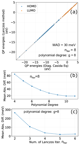
Figure 1: (a). Comparison between the HOMO and LUMO energies calculated with the reference method and the Lanczos method. (b). The mean absolute differences (MAD) between the quasiparticle energies of one hundred small molecules calculated with the reference approach and the Lanczos method with different degrees of polynomial functions; (c). MAD of quasiparticle energies calculated with the reference method and the Lanczos method using different numbers of iterations $N_{\mathrm{iter}}$;

The accuracy of the Lanczos-based method for the $GW$ approximation is checked by calculating the highest occupied and lowest unoccupied molecule orbital (HOMO/LUMO) energies of the GW100 set [46, 47, 48, 49], which include 100 small close-shell molecules for benchmarking different implementations of the GW approximation. $G_{0}W_{0}$-level calculations are carried out throughout this work. As studied in previous work, $G_{0}W_{0}$-level calculations depend on the starting point, while quasiparticle self-consistent GW (QSGW) and fully self-consistent GW can alleviate the dependence of calculation results on the starting points [50, 51, 52, 53]. Our new Lanczos method is compatible with QSGW [54] because the accelerated steps (i.e., bypassing the diagonalization of the Casida equation and using the Lanczos method to compute the correlation part of the self-energy) do not interfere with the self-consistent iterations. The Lanczos method only requires the updated quasiparticle energies and wave functions of the current iteration to start the next iteration of GW calculation. A real-space-based pseudo-potential DFT code PARSEC is used in our implementation to efficiently obtain Kohn-Sham orbitals for large finite systems [55, 56]. Fig. 1 (a) shows the results computed with the Lanczos method and the reference agrees well for all GW100 molecules. The mean average difference (MAD) between the results calculated using the reference method, which finds the eigenpairs of the Casida equation explicitly, and the Lanczos method is within 20 meV. Our tests also show the Lanczos-based formalism converges fast to the degree $g$ of polynomial $p_{g}$ and the number of Lanczos iterations $N_{\textrm{iter}}$. As shown in Fig. 1 (b) and (c), the MAD is below 30 meV when the polynomial degree $g\geq 8$ and $N_{\textrm{iter}}\geq 5$.

The computationally expensive steps in our method are: (1) calculating electron-repulsion integrals $(kl|nm)$ and (2) calculating the matrix-vector product $\mathbf{D}|\star\rangle$, where $|\star\rangle$ is a general vector. One can use suitable low-rank approximation methods, such as resolution-of-identity or density-fitting methods [57, 58, 59], to speed up these computations. Density-fitting methods exploit the rank deficiency of orbital pair products $\phi_{n}(\mathbf{r})\phi_{m}(\mathbf{r})$ and use a set of auxiliary basis functions $\zeta_{\mu}(\mathbf{r})$ to fit these orbital pairs

$$\phi_{n}(\mathbf{r})\phi_{m}(\mathbf{r})\approx\sum_{\mu=1}^{N_{\mu}}\zeta_{\mu}(\mathbf{r})\mathcal{C}^{\mu}_{nm}$$ (15)

where the required number of auxiliary basis functions $N_{\mu}$ for accurately representing the orbital pairs is expected to be small and scale as $O(N)$ and $\mathcal{C}^{\mu}_{nm}$ are fitting coefficients. With the approximation given in Eq. 15, one can calculate integrals $(kl|nm)$, which contribute to the elements of $\mathbf{C}$ and $\mathbf{D}$, with the following equations

$$(kl|nm)\approx\sum_{\alpha=1}^{N_{\mu}}\sum_{\beta=1}^{N_{\mu}}(\alpha|\beta)\mathcal{C}^{\alpha}_{kl}\mathcal{C}^{\beta}_{nm}$$ (16)

$$(\alpha|\beta)=\int\frac{\zeta_{\alpha}(\mathbf{r})\zeta_{\beta}(\mathbf{r}^{\prime})}{|\mathbf{r}-\mathbf{r}^{\prime}|}d^{3}rd^{3}r^{\prime}.$$ (17)

These methods reduce four-center integrals to two-center integrals and also factorize $\mathbf{C}$ and $\mathbf{D}$ as products of small matrices to accelerate the matrix-vector products. We used the interpolative separable density fitting (ISDF) method in our implementation [60, 13, 59]. One can further exploit the point-group symmetries to make the matrix $\mathbf{C}$ block diagonal and simplify the calculation of matrix-vector products [61].

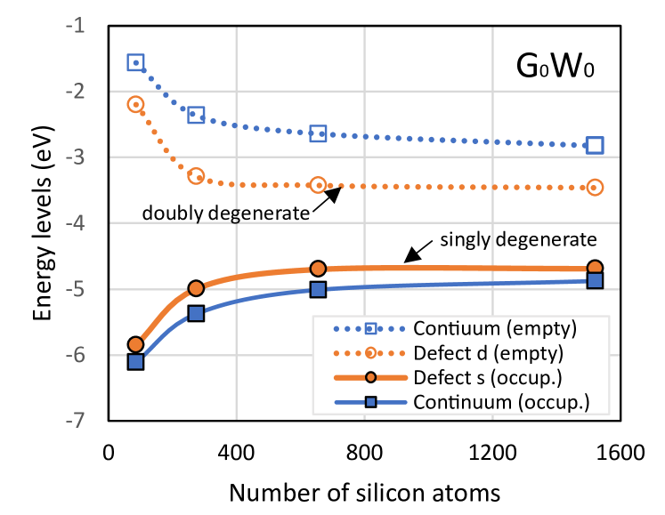
Figure 2: Evolution of “continuum” states and silicon-vacancy defect states in different-sized silicon clusters.

Combined with the ISDF method [13], our method is efficient and enables large-scale $G_{0}W_{0}$ computations with modest computing resources. To demonstrate the efficiency of our method, we performed calculations for hydrogen-passivated silicon clusters with a diameter of up to around 4 nm. Silicon clusters have attracted research interest as prototypical semiconducting clusters for studying the fundamental physical properties of zero-dimensional systems [62] and their applications in many fields [63, 64, 65, 66]. Defects in passivated silicon nanocrystals can introduce mid-gap defect levels as potential sources of photoluminescence [67, 68], while their electronic structures are rarely studied by GW calculations. We computed the defect energy levels of charge-neutral silicon vacancies in silicon clusters of different sizes. The ground state of a silicon vacancy has zero net spin. Different from nano-diamondoids, where surface states are located in the gap, the surface states of silicon nanoclusters are mixed with continuum states and the mid-gap states originate from defects. In the single-particle level, an occupied singlet and a pair of unoccupied doubly degenerate defect states are located inside the gap [69]. As shown in Fig. 2, when the size of silicon clusters increases, the energies of defect states evolve at a similar rate as the continuum states. For the Si₁₅₂₂H₅₂₄ cluster, the band gap of continuum states is around 2.3 eV, still far from the bulk silicon band gap of 1.1 eV. We also computed the HOMO-LUMO gap of non-defective silicon nanocrystals, and our results agree well with previous calculations [36, 70] (See Table S1 in Supplemental Material for details).

Nanocluster	$N_{v}$	$N_{c}+N_{v}$	$N_{\mu}$	$N_{\mathbf{node}}$	$t_{\mathrm{wall}}$ (hr)
Si86H76	210	1730	7000	1	0.02
Si274H172	634	5200	20000	2	0.3
Si452H228	1018	8200	32000	2	0.7
Si656H300	1462	12000	48000	2	1.5
Si1522H524	3306	27000	108000	10	8.5
Si1947H604	4196	33400	133600	20	9.2

Table 1: The running time $t_{\mathrm{wall}}$ and the number of compute nodes $N_{\mathrm{node}}$ for calculating one GW quasiparticle energy. Each compute node has 64 cores and 4 graphic processing units (GPU). $t_{\mathrm{wall}}$ includes the running time for performing the ISDF method and computing $\Sigma^{\mathbf{GW}}(\omega)$ using the Lanczos method. $N_{\mathbf{iter}}=8$ and $g=7$ are used for Lanczos iterations and polynomial functions, respectively.

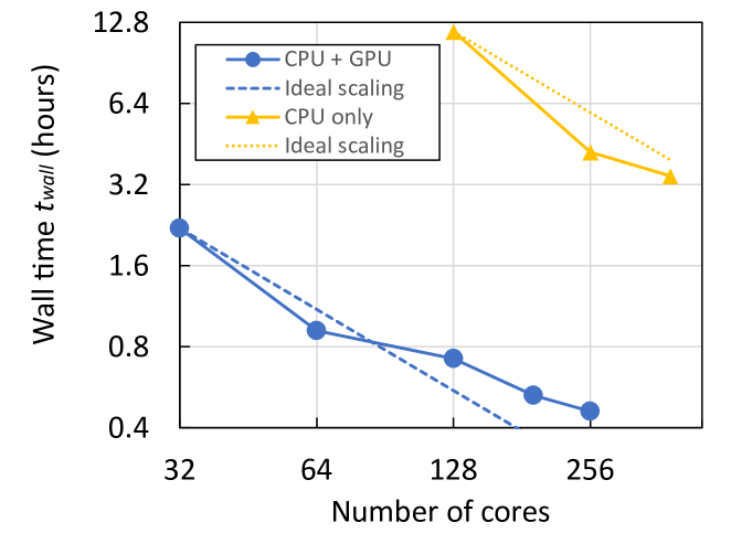
Figure 3: Wall time for computing a GW energy for Si₄₅₂H₂₂₈ cluster with different numbers of CPU cores and GPUs (Nvidia A100). Every compute node has an EPYC 7763 CPU with 64 cores. For the calculations accelerated with GPUs, every 16 CPU cores share 1 GPU processor.

The main calculation parameters and required computation resources for these calculations are shown in Table 1. Notably, only two computing nodes are required for Si₆₅₆H₃₀₀. For the largest system Si₁₉₅₃H₆₀₄ with a diameter of around 4 nm, we used 20 nodes to accomplish the GW calculation. The computational cost of our algorithm has a theoretical scaling of $O(N^{4})$ (a detailed analysis of the computational cost is in the Supplementary material). In the benchmarks of silicon clusters, we observe a practical scaling of roughly $O(N^{2.3})$ for systems with less than 600 silicon atoms. As shown in Fig. 3, we compared the running time for GW calculations of Si₄₅₃H₂₂₈ using different numbers of nodes. Since the most time-consuming step is matrix-matrix and matrix-vector multiplications, our method is suitable for acceleration with GPUs and also demonstrates reasonably good scaling with computation resources. With GPU-accelerated nodes, the speed-up factors are around 20.

In summary, a full-frequency GW formalism based on a Lanczos method is proposed to realize efficient modeling of hundreds of atoms with modest resources. This method can be used for highly efficient full-frequency GW calculations of large finite systems, such as semiconductor quantum dots and ligand-protected superatomic clusters with a few hundred atoms. Our method can also facilitate the construction of computational databases with quasiparticle-energy data, which were challenging to accomplish with limited computational costs before. This method is ready to generalize to extended systems, for which complex-valued wave functions are required. If the Tamm-Dancoff approximation is used (i.e., dropping matrix $\mathbf{B}$ in the Casida equation) for extended systems, then the calculation is greatly simplified as only a Hermitian matrix $\mathbf{A}$ remains and a standard Lanczos algorithm for Hermitian matrix can be used. On the other hand, if RPA is used, then a Lanczos-based method designed for pseudo-Hermitian matrices [33, 71, 35] should be adopted.

I Acknowledgement

This work is supported by the National Natural Science Foundation of China (12104080, 91961204), GHfund A (2022201, ghfund202202012538), the Fundamental Research Funds for the Central Universities (DUT22LK04 and DUT22ZD103), and a sub-award from the Center for Computational Study of Excited-State Phenomena in Energy Materials at the Lawrence Berkeley National Laboratory, which is funded by the U.S. Department of Energy, Office of Science, Basic Energy Sciences, Materials Sciences and Engineering Division under Contract No. DEAC02-05CH11231, as part of the Computational Materials Sciences Program. Computational resources are provided by the Perlmutter supercomputer cluster of the National Energy Research Scientific Computing Center (NERSC), the Sugon Supercomputer Center at Wuzhen, and the Sugon Supercomputer Center at Kunshan.

References

- Hedin [1965] L. Hedin, Phys. Rev. 139, A796 (1965).
- Hybertsen and Louie [1986] M. S. Hybertsen and S. G. Louie, Phys. Rev. B 34, 5390 (1986).
- Godby et al. [1988] R. W. Godby, M. Schlüter, and L. J. Sham, Phys. Rev. B 37, 10159 (1988).
- Rohlfing and Louie [1998] M. Rohlfing and S. G. Louie, Phys. Rev. Lett. 81, 2312 (1998).
- Albrecht et al. [1998] S. Albrecht, L. Reining, R. Del Sole, and G. Onida, Phys. Rev. Lett. 80, 4510 (1998).
- Chan et al. [2021] Y.-H. Chan, D. Y. Qiu, F. H. da Jornada, and S. G. Louie, Proceedings of the National Academy of Sciences 118, e1906938118 (2021).
- Biermann et al. [2003] S. Biermann, F. Aryasetiawan, and A. Georges, Phys. Rev. Lett. 90, 086402 (2003).
- Sun and Kotliar [2002] P. Sun and G. Kotliar, Phys. Rev. B 66, 085120 (2002).
- Zhu and Chan [2021] T. Zhu and G. K.-L. Chan, Phys. Rev. X 11, 021006 (2021).
- Li et al. [2019] Z. Li, G. Antonius, M. Wu, F. H. da Jornada, and S. G. Louie, Phys. Rev. Lett. 122, 186402 (2019).
- Li et al. [2021] Z. Li, M. Wu, Y.-H. Chan, and S. G. Louie, Phys. Rev. Lett. 126, 146401 (2021).
- Golze et al. [2019] D. Golze, M. Dvorak, and P. Rinke, Frontiers in Chemistry 7, 377 (2019).
- Gao et al. [2022] W. Gao, W. Xia, P. Zhang, J. R. Chelikowsky, and J. Zhao, Electronic Structure 4, 023003 (2022).
- Wilhelm et al. [2018] J. Wilhelm, D. Golze, L. Talirz, J. Hutter, and C. A. Pignedoli, The Journal of Physical Chemistry Letters 9, 306 (2018).
- Vlček et al. [2018] V. Vlček, W. Li, R. Baer, E. Rabani, and D. Neuhauser, Phys. Rev. B 98, 075107 (2018).
- Ben et al. [2020] M. D. Ben, C. Yang, Z. Li, F. H. d. Jornada, S. G. Louie, and J. Deslippe, in SC20: International Conference for High Performance Computing, Networking, Storage and Analysis (2020) pp. 1–11.
- Duchemin and Blase [2021] I. Duchemin and X. Blase, Journal of Chemical Theory and Computation 17, 2383 (2021).
- Yu and Govoni [2022] V. W.-z. Yu and M. Govoni, Journal of Chemical Theory and Computation 18, 4690 (2022).
- Deslippe et al. [2012] J. Deslippe, G. Samsonidze, D. A. Strubbe, M. Jain, M. L. Cohen, and S. G. Louie, Computer Physics Communications 183, 1269 (2012).
- Sangalli et al. [2019] D. Sangalli, A. Ferretti, H. Miranda, C. Attaccalite, I. Marri, E. Cannuccia, P. Melo, M. Marsili, F. Paleari, A. Marrazzo, G. Prandini, P. Bonfà, M. O. Atambo, F. Affinito, M. Palummo, A. Molina-Sánchez, C. Hogan, M. Grüning, D. Varsano, and A. Marini, Journal of Physics: Condensed Matter 31, 325902 (2019).
- Hedin [1999] L. Hedin, Journal of Physics: Condensed Matter 11, R489 (1999).
- Casida [1995] M. E. Casida, in Recent Advances in Density Functional Methods, edited by D. P. Chong (World Scientific, 1995) pp. 155–192.
- Bruneval et al. [2016] F. Bruneval, T. Rangel, S. M. Hamed, M. Shao, C. Yang, and J. B. Neaton, Computer Physics Communications 208, 149 (2016).
- Tiago and Chelikowsky [2006] M. L. Tiago and J. R. Chelikowsky, Phys. Rev. B 73, 205334 (2006).
- van Setten et al. [2013] M. J. van Setten, F. Weigend, and F. Evers, Journal of Chemical Theory and Computation 9, 232 (2013).
- Mejia-Rodriguez et al. [2021] D. Mejia-Rodriguez, A. Kunitsa, E. Aprà, and N. Govind, Journal of Chemical Theory and Computation 17, 7504 (2021).
- Onida et al. [2002] G. Onida, L. Reining, and A. Rubio, Rev. Mod. Phys. 74, 601 (2002).
- Haydock [1980] R. Haydock, Computer Physics Communications 20, 11 (1980).
- Meyer and Pal [1989] H. Meyer and S. Pal, The Journal of Chemical Physics 91, 6195 (1989).
- Malcıoğlu et al. [2011] O. B. Malcıoğlu, R. Gebauer, D. Rocca, and S. Baroni, Computer Physics Communications 182, 1744 (2011).
- Walker et al. [2006] B. Walker, A. M. Saitta, R. Gebauer, and S. Baroni, Phys. Rev. Lett. 96, 113001 (2006).
- Zamok et al. [2022] L. Zamok, S. Coriani, and S. P. A. Sauer, The Journal of Chemical Physics 156, 014102 (2022).
- Grüning et al. [2011] M. Grüning, A. Marini, and X. Gonze, Computational Materials Science 50, 2148 (2011).
- Benedict et al. [1998] L. X. Benedict, E. L. Shirley, and R. B. Bohn, Phys. Rev. B 57, R9385 (1998).
- Shao et al. [2018] M. Shao, F. H. da Jornada, L. Lin, C. Yang, J. Deslippe, and S. G. Louie, SIAM Journal on Matrix Analysis and Applications 39, 683 (2018).
- Govoni and Galli [2015] M. Govoni and G. Galli, Journal of Chemical Theory and Computation 11, 2680 (2015).
- Umari et al. [2010] P. Umari, G. Stenuit, and S. Baroni, Phys. Rev. B 81, 115104 (2010).
- Laflamme Janssen et al. [2015] J. Laflamme Janssen, B. Rousseau, and M. Côté, Phys. Rev. B 91, 125120 (2015).
- Bintrim and Berkelbach [2021] S. J. Bintrim and T. C. Berkelbach, The Journal of Chemical Physics 154, 041101 (2021).
- Scott et al. [2023] C. J. C. Scott, O. J. Backhouse, and G. H. Booth, The Journal of Chemical Physics 158, 124102 (2023).
- Backhouse et al. [2021] O. J. Backhouse, A. Santana-Bonilla, and G. H. Booth, The Journal of Physical Chemistry Letters 12, 7650 (2021).
- Chiarotti et al. [2022] T. Chiarotti, N. Marzari, and A. Ferretti, Phys. Rev. Res. 4, 013242 (2022).
- Leon et al. [2023] D. A. Leon, A. Ferretti, D. Varsano, E. Molinari, and C. Cardoso, Phys. Rev. B 107, 155130 (2023).
- Bintrim and Berkelbach [2022] S. J. Bintrim and T. C. Berkelbach, The Journal of Chemical Physics 156, 044114 (2022).
- Schirmer et al. [1983] J. Schirmer, L. S. Cederbaum, and O. Walter, Phys. Rev. A 28, 1237 (1983).
- van Setten et al. [2015] M. J. van Setten, F. Caruso, S. Sharifzadeh, X. Ren, M. Scheffler, F. Liu, J. Lischner, L. Lin, J. R. Deslippe, S. G. Louie, C. Yang, F. Weigend, J. B. Neaton, F. Evers, and P. Rinke, Journal of Chemical Theory and Computation 11, 5665 (2015).
- Govoni and Galli [2018] M. Govoni and G. Galli, Journal of Chemical Theory and Computation 14, 1895 (2018).
- Förster and Visscher [2021] A. Förster and L. Visscher, Journal of Chemical Theory and Computation 17, 5080 (2021).
- Gao and Chelikowsky [2019] W. Gao and J. R. Chelikowsky, Journal of Chemical Theory and Computation 15, 5299 (2019).
- Caruso et al. [2013] F. Caruso, P. Rinke, X. Ren, A. Rubio, and M. Scheffler, Phys. Rev. B 88, 075105 (2013).
- Marom et al. [2012] N. Marom, F. Caruso, X. Ren, O. T. Hofmann, T. Körzdörfer, J. R. Chelikowsky, A. Rubio, M. Scheffler, and P. Rinke, Phys. Rev. B 86, 245127 (2012).
- Rinke et al. [2005] P. Rinke, A. Qteish, J. Neugebauer, C. Freysoldt, and M. Scheffler, New Journal of Physics 7, 126 (2005).
- Dauth et al. [2016] M. Dauth, F. Caruso, S. Kümmel, and P. Rinke, Phys. Rev. B 93, 121115 (2016).
- Hung et al. [2016] L. Hung, F. H. da Jornada, J. Souto-Casares, J. R. Chelikowsky, S. G. Louie, and S. Öğüt, Phys. Rev. B 94, 085125 (2016).
- Kronik et al. [2006] L. Kronik, A. Makmal, M. L. Tiago, M. M. G. Alemany, M. Jain, X. Huang, Y. Saad, and J. R. Chelikowsky, Phys. Status Solidi B 243, 1063 (2006).
- Dogan et al. [2023] M. Dogan, K.-H. Liou, and J. R. Chelikowsky, Phys. Rev. Mater. 7, L063001 (2023).
- Weigend [2002] F. Weigend, Phys. Chem. Chem. Phys. 4, 4285 (2002).
- Ren et al. [2012] X. Ren, P. Rinke, V. Blum, J. Wieferink, A. Tkatchenko, A. Sanfilippo, K. Reuter, and M. Scheffler, New Journal of Physics 14, 053020 (2012).
- Hu et al. [2020] W. Hu, J. Liu, Y. Li, Z. Ding, C. Yang, and J. Yang, Journal of Chemical Theory and Computation 16, 964 (2020).
- Lu and Ying [2015] J. Lu and L. Ying, Journal of Computational Physics 302, 329 (2015).
- Gao and Chelikowsky [2020] W. Gao and J. R. Chelikowsky, Journal of Chemical Theory and Computation 16, 2216 (2020).
- Barbagiovanni et al. [2014] E. G. Barbagiovanni, D. J. Lockwood, P. J. Simpson, and L. V. Goncharova, Applied Physics Reviews 1, 011302 (2014).
- Liang et al. [2019] J. Liang, C. Huang, and X. Gong, ACS Sustainable Chemistry & Engineering 7, 18213 (2019).
- Dohnalová et al. [2013] K. Dohnalová, A. N. Poddubny, A. A. Prokofiev, W. D. de Boer, C. P. Umesh, J. M. Paulusse, H. Zuilhof, and T. Gregorkiewicz, Light: Science & Applications 2, e47 (2013).
- Neiner et al. [2006] D. Neiner, H. W. Chiu, and S. M. Kauzlarich, Journal of the American Chemical Society 128, 11016 (2006).
- Huan and Shu-Qing [2014] C. Huan and S. Shu-Qing, Chinese Physics B 23, 088102 (2014).
- Godefroo et al. [2008] S. Godefroo, M. Hayne, M. Jivanescu, A. Stesmans, M. Zacharias, O. I. Lebedev, G. Van Tendeloo, and V. V. Moshchalkov, Nature Nanotechnology 3, 174 (2008).
- Priolo et al. [2014] F. Priolo, T. Gregorkiewicz, M. Galli, and T. F. Krauss, Nature Nanotechnology 9, 19 (2014).
- Liao et al. [2022] T. Liao, K.-H. Liou, and J. R. Chelikowsky, Phys. Rev. Mater. 6, 054603 (2022).
- Neuhauser et al. [2014] D. Neuhauser, Y. Gao, C. Arntsen, C. Karshenas, E. Rabani, and R. Baer, Phys. Rev. Lett. 113, 076402 (2014).
- Brabec et al. [2015] J. Brabec, L. Lin, M. Shao, N. Govind, C. Yang, Y. Saad, and E. G. Ng, Journal of Chemical Theory and Computation 11, 5197 (2015).