Data Market Design through Deep Learning

Abstract

The data market design problem is a problem in economic theory to find a set of signaling schemes (statistical experiments) to maximize expected revenue to the information seller, where each experiment reveals some of the information known to a seller and has a corresponding price (Bergemann et al., 2018). Each buyer has their own decision to make in a world environment, and their subjective expected value for the information associated with a particular experiment comes from the improvement in this decision and depends on their prior and value for different outcomes. In a setting with multiple buyers, a buyer’s expected value for an experiment may also depend on the information sold to others (Bonatti et al., 2022). We introduce the application of deep learning for the design of revenue-optimal data markets, looking to expand the frontiers of what can be understood and achieved. Relative to earlier work on deep learning for auction design (Dütting et al., 2023), we must learn signaling schemes rather than allocation rules and handle obedience constraints $-$ these arising from modeling the downstream actions of buyers $-$ in addition to incentive constraints on bids. Our experiments demonstrate that this new deep learning framework can almost precisely replicate all known solutions from theory, expand to more complex settings, and be used to establish the optimality of new designs for data markets and make conjectures in regard to the structure of optimal designs.

1 Introduction

Many characterize the current era as the Information Age. Companies such as Google and Meta (search and social media), Experian and TransUnion (credit agencies), and Amazon and American Express (commerce) hold vast quantities of data about individuals. In turn, this has led to data markets, where information about an individual can be purchased in real-time to guide decision-making (e.g., LiveRamp, Segment, Bloomreach). In this paper, we advance the design of market rules that govern the structuring and sale of this kind of information. Using machine learning, we leverage existing theoretical frameworks (Bergemann et al., 2018; Bonatti et al., 2022) to replicate all known solutions from theory, expand to more complex settings, establish the optimality of new designs, and make conjectures in regard to the structure of optimal designs. Although this is not our focus, there are also important ethical questions in regard to data markets, in regard to privacy, ownership, informed consent, and the use of data (Acquisti et al., 2016; Bonatti, 2022; Bergemann et al., 2022a; Athey et al., 2017; Choi et al., 2019; Fainmesser et al., 2022; Acemoglu et al., 2022).

In settings with a single buyer, Bergemann et al. (2018) introduce a framework in which there is a data buyer who faces a decision problem under uncertainty, and has a payoff depending on their choice of action and the underlying state of the world. There is a data seller who knows the world state, and can disclose information through a menu of statistical experiments, each experiment offering a stochastic signal that reveals some (or all) of the seller’s information and each of which is associated with a price. The buyer’s willingness to pay for information is determined by their type, which defines their prior belief and their value for different outcomes in the world (these arising from the action that the buyer will choose to take).

The optimal data market design problem is to find a set of experiments and associated prices with which to maximize expected revenue, given a distribution over the buyer’s type. Bergemann et al. (2018) characterize the optimal design when there is a binary world state and a buyer with a binary action. In some settings there may be multiple buyers and buyers may compete downstream, and the more informed one buyer is, the lower the payoff may become for others. Bonatti et al. (2022) take up this problem, and characterize the optimal design for multiple buyers in the binary state/binary action setting, and further limited to buyers who each have a common prior on the world state. It remains an open problem to obtain theoretical results for richer, multi-buyer settings, and this motivates the need for gaining new understanding and making progress through computational approaches.

1.1 Contributions

Inspired by the recent advances in differential economics (Dütting et al. (2023); Feng et al. (2018); Golowich et al. (2018); Kuo et al. (2020); Ravindranath et al. (2021); Tacchetti et al. (2019); Peri et al. (2021); Rahme et al. (2021); Curry et al. (2020, 2022); Duan et al. (2022); Ivanov et al. (2022); Curry et al. (2023); Duan et al. (2023) etc.), we initiate the use of deep learning for the automated design of data markets. This market sells information rather than allocates resources, and the value of information depends on the way in which a buyer will use the information—and this downstream action by a buyer needs to be modeled. Following the revelation principle for dynamic games (Myerson (1991), Section 6.3), it is without loss of generality to model an experiment as generating a recommended action and insisting on designs in which the buyer will prefer to follow this action. This brings about new challenges, most notably to extend this framework to handle obedience. While the other aspect of incentive compatibility that we need to handle is more typical, i.e., that of achieving incentive alignment so that a buyer will choose to truthfully report their prior beliefs and values for different outcomes, we also need to ensure there are no useful double deviations, where a buyer simultaneously misreports their type and acts contrary to the seller’s recommended action.

In settings with a single buyer, we learn an explicit, parameterized representation of a menu of priced experiments to offer the buyer and with which to model the action choices available to the buyer. In this way, we extend the RochetNet architecture Dütting et al. (2023) that has been used successfully for optimal auction design with a single buyer. This enables us to obtain exact incentive compatibility for the single buyer setting: a buyer has no useful deviation from a recommended action, no useful deviation in reporting their type, and no useful double deviation. In settings with multiple buyers, we seek to learn revenue-maximizing designs while also minimizing deviations in disobeying action recommendations and misreporting types and including double deviations. This extends the RegretNet framework Dütting et al. (2023) that has been used successfully for optimal auction design with multiple buyers and gives approximate incentive alignment.

Our first experimental result is to show through extensive experiments that these new neural network architectures and learning frameworks are able to almost exactly recover all known optimal solutions from Bergemann et al. (2018) and Bonatti et al. (2022). Following the economic theory literature on data market design, we consider the notion of Bayesian incentive compatibility (BIC). To handle this, we use samples of a buyer’s type to compute an interim experiment and interim payment, averaging over samples drawn from the type distribution (this builds on the BIC methods for deep learning for auctions that were used in the context of differentiable economics for budget-constrained auctions Feng et al. (2018)). We give a training method that enables the efficient reuse of computed interim allocations and interim payments from other samples to swiftly calculate the interim utility of misreports, dramatically speeding up training.

Whereas analytical results are only available for the BIC setting, which is, in effect, lower-dimensional, and easier to analyze, we are able to study through computational techniques the design of data markets in the ex post IC setting, which is a setting without existing theory. A second result, in the setting of multiple buyers, is to use our framework to conjecture the structure of an optimal design and prove its optimality (for this, we make use of virtual values analogous to Myerson’s framework Myerson (1981)). We see this as an important contribution, as ex post IC is a stronger notion of IC than BIC.

A third result is to demonstrate how our framework extends its utility beyond empirical results and serves as a toolbox to guide economic theory. To illustrate this, we study how revenue varies with competition in the multi-buyer setting where the prior information is uncertain. Despite the absence of existing theoretical results for this particular setting, our framework enables us to derive trends in revenue effortlessly. We also conjecture the structure of solutions for problems in the single buyer setting with an enlarged type, where both the buyer payoffs and priors are uncertain. For this case, we again derive empirical results using our proposed framework and use it to conjecture the properties of the underlying theoretical solution.

1.2 Related work

Conitzer and Sandholm (2002, 2004) introduced the use of automated mechanism design (AMD) for economic design and framed the problem as an integer linear program (or just a linear program for Bayesian design). Responding to challenges with the enumerative representations used in these early approaches,  Dütting et al. (2023) introduced the use of deep neural networks for auction design, attaining more representational flexibility. Since then, there has been a line of work on this so-called approach of differentiable economics, including to problems with budget-constrained bidders (Feng et al., 2018), for minimizing agents’ payments (Tacchetti et al., 2019), applying to multi-facility location problems (Golowich et al., 2018), balancing fairness and revenue (Kuo et al., 2020), and applying to two-sided matching (Ravindranath et al., 2021). To the best of our knowledge, none of this work has considered the setting of the design of optimal data markets, which introduce new challenges in regard to handling agent actions (obedience) as well as incorporating negative externalities.

In regard to the data market problem, Bergemann et al. (2018) build upon the decision-theoretic model pioneered by Blackwell (1953) and study a setting with a single buyer. Cai and Velegkas (2021) also give computational results in this model, making use of linear programs to compute the optimal menu for discrete type distributions. They also investigate a generalization of this model that allows multiple agents to compete for useful information. In this setting, at most, one agent receives the information. While this approach can be used for continuous type distribution by applying the LP to a discretized valuation space, solving it for even a coarser discretization can be prohibitively expensive. Further advancing economic theory, Bergemann et al. (2022b) consider more general type distributions and investigate both the cardinality of the optimal menu and the revenue achievable when selling complete information. Bonatti et al. (2022) also study the multi-buyer setting modelling competition through negative externality.

Babaioff et al. (2012) give a related framework, with the key distinction that the seller is not required to commit to a mechanism before the realization of the world state. As a result, the experiments and prices of the data market can be tailored to the realized state of the world. Chen et al. (2020) extend their setting, considering budget-constrained buyers, formulating a linear program to find the solution of the problem for a discrete type space.

There exist several other models that study revenue-optimal mechanisms for selling data. For example, Liu et al. (2021) characterize the revenue-optimal mechanism for various numbers of states and actions, and consider general payoff functions. However, in their setup, the state only impacts the payoff of the active action taken by a buyer, which provides considerable simplification and may not be realistic. Li (2022) investigates a setting where the buyer can conduct their own costly experiment at a cost after receiving the signal. Different from the model considered in this paper, after receiving the signal from the data broker, the agent can subsequently acquire additional information with costs. The model also assumed that the valuation function of the agent is separable and that the private type of the agent represents her value of acquiring more information, which is different from the single buyer model studied in this paper, where the prior belief is also drawn from a distribution and constitutes a part of the buyer’s type. Agarwal et al. (2019) explore data marketplaces where each of multiple sellers sells data to buyers who aim to utilize the data for machine learning tasks, and Chen et al. (2022) consider scenarios where neither the seller nor the buyer knows the true quality of the data. Mehta et al. (2019) and Agarwal et al. (2020) also incorporate buyer externalities into the study of data marketplaces.

Another line of research studies problems of information design, for example, the problem of Bayesian Persuasion (Kamenica and Gentzkow, 2011). There, the model is different in that the sender of information has preferences on the action taken by the receiver, setting up a game-theoretic problem of strategic misrepresentation by the sender. Dughmi and Xu (2016) studied this from an algorithmic perspective, and Castiglioni et al. (2022) also brought in considerations from mechanism design by introducing hidden types; see also Dughmi (2014), Daskalakis et al. (2016), and Cai et al. (2020) for more work on information design and Bayesian persuasion.

2 Preliminaries

2.1 Model

We consider a setting with $n$ data buyers, $N=\{1,\ldots,n\}$, each facing a decision problem under uncertainty. The state of the world, $\omega$, is unknown and is drawn from a finite state space $\Omega=\{\omega_{1},\ldots\omega_{m}\}$. Each buyer $i$ can choose an action, from a finite set $\mathcal{A}_{i}$. Let $\mathcal{A}=\Pi_{i=1}^{n}\mathcal{A}_{i}$. The ex post payoff to buyer $i$ for choosing action $a_{i}\in\mathcal{A}_{i}$ under state $\omega$ is given by $\mathcal{U}_{i}(\omega,a_{i})$. Unless otherwise specified, we consider the case of matching utility payoffs where the buyer seeks to match the state and the action. In such settings, we have $|\Omega|=|\mathcal{A}_{i}|$ for each $i\in[n]$, and the payoff is given by $\mathcal{U}_{i}(\omega,a_{i})=v_{i}\cdot\mathbf{1}\{\omega=a_{i}\}$ where each $v_{i}$ is drawn independently from a distribution $\mathcal{V}_{i}$. Let $\mathcal{V}=\Pi_{i=1}^{n}\mathcal{V}_{i}$.

Each buyer $i$ also has an interim belief, $\theta_{i}\in\Delta(\Omega)$, about the world state. Each buyer’s belief, $\theta_{i}$, is drawn independently from a distribution $\Theta_{i}$. Let $\Theta=\Pi_{i=1}^{n}\Theta_{i}$. The type of a buyer is given by the tuple $(v_{i},\theta_{i})$ and is denoted by $\rho_{i}$. If the buyers don’t vary in $v_{i}$ or their interim beliefs $\theta_{i}$, then $\rho_{i}=\theta_{i}$ or $\rho_{i}=v_{i}$, respectively. Let $\mathcal{P}_{i}\triangleq\mathcal{V}_{i}\times\Theta_{i}$. The utility of a buyer $i\in[n]$ is given by the utility function $u_{i}:\mathcal{A}\times\Omega\times\mathcal{P}_{i}\to\mathbb{R}$. We assume that the utility of buyer $i$ depends only on its own type $\rho_{i}$ but can depend on other players’ actions as a negative externality. Additionally, we follow Bonatti et al. (2022) and assume that this externality is separable, thus simplifying our utility $u_{i}(a,\omega,\rho_{i})=v_{i}\cdot\mathbf{1}\{a_{i}=\omega\}-E_{-i}(a_{-i},\omega,\rho_{i})$. In this paper, we consider settings where the negative externality is given by $E_{-i}(a_{-i},\omega,\rho_{i})=\frac{\alpha}{n-1}\sum_{j\in[n]\setminus i}v_{i}\cdot\mathbf{1}\{a_{j}=\omega\}$ where $\alpha\in\mathbb{R}_{\geq 0}$ where $\alpha$ captures the degree of competitiveness among buyers. Let $\bar{\alpha}=\frac{\alpha}{n-1}$.

2.2 Statistical Experiments

There is a data seller who observes the world state and wishes to sell information to one or more buyers to maximize expected revenue. The seller sells information through signaling schemes, where each scheme is called an experiment. The seller chooses, for each buyer $i\in[n]$, a set of signals $\mathcal{S}_{i}$ and a signaling scheme $\sigma_{i}:\Omega\to\triangle\mathcal{S}_{i}$. If state $\omega\in\Omega$ is realized, then the seller sends a signal drawn from the distribution $\sigma_{i}(\omega)$. Upon receiving a signal, the buyers update their prior beliefs and choose an optimal action accordingly. The signaling scheme $\sigma_{i}$ can also be represented as a matrix $\pi_{i}$ $-$ a collection of $m$ row vectors each of dimensions $|\mathcal{S}_{i}|$. The $j$-th row vector (for $j\in[m])$ specifies the likelihood of each signal when state $\omega_{j}$ is realized. Thus we have $\sigma_{i}(\omega_{j})=\pi_{i,j}$.

2.3 The Mechanism Design Problem

The mechanism design goal is to design a set of experiments and corresponding prices to maximize the expected revenue of the seller. Let $\mathcal{B}$ denote a message (bid) space. Define the signaling schemes for a buyer $i\in[n]$ as $\sigma_{i}:\Omega\times\mathcal{B}\to\triangle\mathcal{S}_{i}$ and a payment function $t_{i}:\mathcal{B}\to\mathbb{R}_{\geq 0}$. Given bids $b=(b_{1},\ldots b_{n})\in\mathcal{B}$, if state $\omega\in\Omega$ is realized, then the seller sends a signal drawn from the distribution $\sigma_{i}(\omega,b)$ to buyer $i$ and collects payment $t_{i}(b)$. The sequence of interactions between one or more buyers and the seller takes place as follows:

1. The seller commits to a mechanism, $\mathcal{M}=(\sigma,t)$, where $\sigma=(\sigma_{1},\ldots,\sigma_{n})$ is a choice and $t=(t_{1},\ldots,t_{n})$.

2. Each buyer $i$ observes their type, $\rho_{i}$. The seller observes the state, $\omega$.

3. Each buyer reports a message $b_{i}$.

4. The seller sends buyer $i$ a signal, $S_{i}\in\mathcal{S}_{i}$, generated according to the signaling scheme $\sigma_{i}(\omega,b)$, and collects payment $t_{i}(b)$.

5. Each buyer $i$ chooses an action $a_{i}\in\mathcal{A}_{i}$, and obtains utility $u_{i}(a,\omega,V_{i},\theta_{i})-t_{i}(b)$, where $a=(a_{1},\ldots,a_{n})$.

By the revelation principle for dynamic games (Myerson (1991), Section 6.3), as long as we consider incentive-compatible mechanisms, it is without loss of generality for the message space to be the type space of buyers, and for the size of the signal space to be the size of the action space, i.e., for each $i\in[n]$, $|\mathcal{S}_{i}|=|\mathcal{A}_{i}|$. In such mechanisms, the seller designs experiments where every signal leads to a different optimal choice of action. Following Bergemann et al. (2018), we can then replace every signal as an action recommended by the seller.

Incentive Compatibility.

A mechanism $(\sigma,t)$ is Bayesian incentive compatible (BIC) if the buyer maximizes their expected utility (over other agents’ reports) by both reporting their true type as well as by following the recommended actions. For the sake of notational convenience, let $\hat{\mathbb{E}}_{-i}:=\mathop{\mathbb{E}}_{\rho_{-i}\sim\mathcal{P}_{-i}}$ denote the operator used for computing the interim representations. For each $(\rho_{i},\rho_{i}^{\prime})\in\mathcal{P}_{i}^{2}$ and for each deviation function $\delta:\mathcal{A}_{i}\to\mathcal{A}_{i}$, a BIC mechanism satisfies:

$$\hat{\mathbb{E}}_{-i}\left[\mathop{\mathbb{E}}_{\begin{subarray}{c}a\sim\sigma(\omega,\rho)\\ \omega\sim\theta_{i}\end{subarray}}\left[u_{i}(a,\omega,\rho)-t_{i}(\rho)\right]\right]\geq\hat{\mathbb{E}}_{-i}\left[\mathop{\mathbb{E}}_{\begin{subarray}{c}a\sim\sigma(\omega;\rho_{i}^{\prime},\rho_{-i})\\ \omega\sim\theta_{i}\end{subarray}}\left[u_{i}(\delta(a_{i}),a_{-i},\omega,\rho)-t_{i}(\rho_{i}^{\prime},\rho_{-i})\right]\right]$$ (1)

In particular, this insists that double deviations (misreporting the type and disobeying the recommendation) are not profitable. It is helpful to further define the notions of obedience and truthfulness, which consider particular forms of restricted incentive compatibility.

A mechanism $(\sigma,t)$ is obedient if an agent maximizes its expected utility by following the action recommendations assuming all the other agents report their types truthfully and follow the action recommendations. Formally, obedience requires that a mechanism $(\sigma,t)$ satisfies the following condition, for every agent $i$:

$$\hat{\mathbb{E}}_{-i}\left[\mathop{\mathbb{E}}_{\begin{subarray}{c}a\sim\sigma(\omega,\rho),\\ \omega\sim\theta_{i}\end{subarray}}\left[u_{i}(a,\omega,\rho)\right]\right]\geq\hat{\mathbb{E}}_{-i}\left[\mathop{\mathbb{E}}_{\begin{subarray}{c}a\sim\sigma(\omega,\rho),\\ \omega\sim\theta_{i}\end{subarray}}\left[u_{i}(\delta(a_{i}),a_{-i},\omega,\rho)\right]\right]$$ (2)

A mechanism $(\sigma,t)$ is truthful if an agent maximizes its expected utility by reporting its true type, assuming all agents, including itself, are obedient and that the other agents are truthful. Formally, truthfulness requires that a mechanism $(\sigma,t)$ satisfies the following condition, for every agent $i$:

$$\hat{\mathbb{E}}_{-i}\left[\mathop{\mathbb{E}}_{\begin{subarray}{c}a\sim\sigma(\omega,\rho),\\ \omega\sim\theta_{i}\end{subarray}}\left[u_{i}(a,\omega,\rho)-t_{i}(\rho)\right]\right]\geq\hat{\mathbb{E}}_{-i}\left[\mathop{\mathbb{E}}_{\begin{subarray}{c}a\sim\sigma(\omega;\rho_{i}^{\prime},\rho_{-i}),\\ \omega\sim\theta_{i}\end{subarray}\ }\left[u_{i}(a,\omega,\rho)-t_{i}(\rho_{i}^{\prime},\rho_{-i})\right]\right]$$ (3)

We also consider the stronger notion of ex post incentive compatible (IC), which requires, for every agent $i$, and for each $\rho\in\mathcal{P}$, and assuming that every other agent reports its type truthfully and follows the recommended action, then for each each misreport $\rho_{i}^{\prime}\in\mathcal{P}_{i}$, and each deviation function, $\delta:\mathcal{A}_{i}\to\mathcal{A}_{i}$, the following condition:

$$\mathop{\mathbb{E}}_{\begin{subarray}{c}a\sim\sigma(\omega,\rho),\\ \omega\sim\theta_{i}\end{subarray}}\left[u_{i}(a,\omega,\rho)-t_{i}(\rho)\right]\geq\mathop{\mathbb{E}}_{\begin{subarray}{c}a\sim\sigma(\omega;\rho_{i}^{\prime},\rho_{-i}),\\ \omega\sim\theta_{i}\end{subarray}\ }\left[u_{i}(\delta(a_{i}),a_{-i},\omega,\rho)-t_{i}(\rho_{i}^{\prime},\rho_{-i})\right]$$ (4)

In particular, we also say that a mechanism $(\sigma,t)$ is ex post obedient if it satisfies, for every agent $i$:

$$\mathop{\mathbb{E}}_{\begin{subarray}{c}a\sim\sigma(\omega,\rho),\\ \omega\sim\theta_{i}\end{subarray}}\left[u_{i}(a,\omega,\rho)\right]\geq\mathop{\mathbb{E}}_{\begin{subarray}{c}a\sim\sigma(\omega,\rho),\\ \omega\sim\theta_{i}\end{subarray}}\left[u_{i}(\delta(a_{i}),a_{-i},\omega,\rho)\right].$$ (5)

Also, a mechanism is ex post truthful if it satisfies, for every agent $i$:

$$\mathop{\mathbb{E}}_{\begin{subarray}{c}a\sim\sigma(\omega,\rho),\\ \omega\sim\theta_{i}\end{subarray}}\left[u_{i}(a,\omega,\rho)-t_{i}(\rho)\right]\geq\mathop{\mathbb{E}}_{\begin{subarray}{c}a\sim\sigma(\omega;\rho_{i}^{\prime},\rho_{-i}),\\ \omega\sim\theta_{i}\end{subarray}\ }\left[u_{i}(a,\omega,\rho)-t_{i}(\rho_{i}^{\prime},\rho_{-i})\right]$$ (6)

Individual Rationality. A mechanism is interim individually rational (IIR) if reporting an agent’s true type guarantees at least as much expected utility (in expectation over other agents’ reports) as opting out of the mechanism. Let $\sigma_{-i}:\Omega\times\mathcal{P}_{-i}\to\triangle\mathcal{A}_{-i}$ denote the recommendations to other participating buyers when buyer $i$ opts out. For each agent $i$, and each $\rho_{i}\in\mathcal{P}_{i}$, IIR requires

$$\hat{\mathbb{E}}_{-i}\left[\mathop{\mathbb{E}}_{\begin{subarray}{c}a\sim\sigma(\omega;\rho),\\ \omega\sim\theta_{i}\end{subarray}}\left[u_{i}(a;\omega,\rho)-t_{i}(\rho)\right]\right]\geq\max_{\tilde{a}_{i}\in\mathcal{A}_{i}}\hat{\mathbb{E}}_{-i}\left[\mathop{\mathbb{E}}_{\begin{subarray}{c}a_{-i}\sim\sigma_{-i}(\omega;\rho_{-i}),\\ \omega\sim\theta_{i}\end{subarray}}\left[u_{i}(\tilde{a}_{i},a_{-i};\omega,\rho)\right]\right]\$$ (7)

It is in the seller’s best interest to instantiate the recommendation function to the other buyers when buyer $i$ opts out, $\sigma_{-i}$, to minimize the value of the RHS of this IIR inequality. For this reason, it is without loss of generality to rewrite the above equation as:

$$\hat{\mathbb{E}}_{-i}\left[\mathop{\mathbb{E}}_{\begin{subarray}{c}a\sim\sigma(\omega;\rho),\\ \omega\sim\theta_{i}\end{subarray}}\left[u_{i}(a;\omega,\rho)-t_{i}(\rho)\right]\right]\geq\min_{\sigma_{-i}}\max_{\tilde{a}_{i}\in\mathcal{A}_{i}}\left(\mathbb{E}_{-i}\left[\mathop{\mathbb{E}}_{\begin{subarray}{c}a\sim\sigma_{-i}(\omega;\rho_{-i}),\\ \omega\sim\theta_{i}\end{subarray}}\left[u_{i}(\tilde{a}_{i},a_{-i};\omega,\rho)\right]\right]\right)$$ (8)

In particular, and recognizing that a buyer’s utility decreases the more informed other buyers are, the seller can achieve this by sending optimal recommendations to participating buyers in order to minimize the utility of a non-participating buyer.

We also consider a stronger version of IR, namely ex post individual rationality (or simply IR). In this case, for each agent $i$, and each $\rho\in\mathcal{P}$, we require:

$$\mathop{\mathbb{E}}_{\begin{subarray}{c}a\sim\sigma(\omega;\rho),\\ \omega\sim\theta_{i}\end{subarray}}\left[u_{i}(a;\omega,\rho)-t_{i}(\rho)\right]\geq\min_{\sigma_{-i}}\max_{\tilde{a}_{i}\in\mathcal{A}_{i}}\left(\mathop{\mathbb{E}}_{\begin{subarray}{c}a\sim\sigma_{-i}(\omega;\rho_{-i}),\\ \omega\sim\theta_{i}\end{subarray}}\left[u_{i}(\tilde{a}_{i},a_{-i};\omega,\rho)\right]\right)$$ (9)

2.4 Illustrative Example

Example 1.

Consider a setting with $n=2$ buyers, two states of the world $\Omega=\{0,1\}$ and two actions for each buyer $\mathcal{A}_{1}=\mathcal{A}_{2}=\{0,1\}$. Let $\Theta_{1},\Theta_{2}$ be singleton sets with $\Theta_{1}=\Theta_{2}=\{(0.3,0.7)\}$. Let $\mathcal{V}_{1}=\mathcal{V}_{2}=U[0,1]$. Since the priors are fixed, the agents types are just represented by $v_{i}$ i.e, we have $\rho_{i}=v_{i}$. The utility function $u_{i}$ is given by

$$u_{i}(a_{i},a_{-i};\omega,v_{i})=v_{i}\left(\mathbf{1}\{a_{i}=\omega\}-\alpha\mathbf{1}\{a_{-i}=\omega\}\right)$$ (10)

for some $\omega\in\Omega$. In each state of the world, the dominant strategy is to play the state matching the action. Buyer $i$ also incurs a negative externality if the other buyer (denoted by $-i$) chooses the correct action. The intensity of the negative externality is captured by the parameter $\alpha\in\mathbb{R}_{\geq 0}$.

Consider a signaling scheme that always recommends action $1$ with probability $0.9$ if $\omega=0$ and $0.2$ if $\omega=1$. This experiment can be represented as follows:

$$\pi_{i}(v)=\begin{pmatrix}0.1&0.9\\ 0.8&0.2\end{pmatrix}$$ (11)

Obedience:

The expected utility from the experiment for each agent, if they are obedient, is given by:

$$\mathop{\mathbb{E}}_{\begin{subarray}{c}a\sim\sigma_{i},\\ \omega\sim\theta_{i}\end{subarray}}[u_{i}(a_{i},a_{-i};\omega,v_{i})] =\mathop{\mathbb{E}}_{\begin{subarray}{c}a\sim\sigma_{i},\\ \omega\sim\theta_{i}\end{subarray}}[v_{i}\left(\mathbf{1}\{a_{i}=\omega\}-\alpha\mathbf{1}\{a_{-i}=\omega\}\right)]$$ (12)

$$=v_{i}\left(\sum_{j=0}^{1}\text{Pr}[\omega=j]\text{Pr}[a_{i}=j\mid\omega=j]\right)-v_{i}\alpha\mathop{\mathbb{E}}_{\begin{subarray}{c}a\sim\sigma_{i},\\ \omega\sim\theta_{i}\end{subarray}}[\mathbf{1}\{a_{-i}=\omega\}]$$

$$=0.17v_{i}-v_{i}\alpha\mathop{\mathbb{E}}_{\begin{subarray}{c}a\sim\sigma_{i},\\ \omega\sim\theta_{i}\end{subarray}}[\mathbf{1}\{a_{-i}=\omega\}]$$

Consider the following deviation function $\delta$ such that the agent takes the exact opposite action of what is recommended i.e., $\delta(j)=1-j$. The utility for each agent under such deviation is given by:

$$\mathop{\mathbb{E}}_{\begin{subarray}{c}a\sim\sigma_{i},\\ \omega\sim\theta_{i}\end{subarray}}[u_{i}(\delta(a_{i}),a_{-i};\omega,v_{i})] =\mathop{\mathbb{E}}_{\begin{subarray}{c}a\sim\sigma_{i},\\ \omega\sim\theta_{i}\end{subarray}}[v_{i}\left(\mathbf{1}\{\delta(a_{i})=\omega\}-\alpha\mathbf{1}\{a_{-i}=\omega\}\right)]$$ (13)

$$=v_{i}\left(\sum_{j=0}^{1}\text{Pr}[\omega=j]\text{Pr}[a_{i}=1-j\mid\omega=j]\right)-v_{i}\alpha\mathop{\mathbb{E}}_{\begin{subarray}{c}a\sim\sigma_{i},\\ \omega\sim\theta_{i}\end{subarray}}[\mathbf{1}\{a_{-i}=\omega\}]$$

$$=0.83v_{i}-v_{i}\alpha\mathop{\mathbb{E}}_{\begin{subarray}{c}a\sim\sigma_{i},\\ \omega\sim\theta_{i}\end{subarray}}[\mathbf{1}\{a_{-i}=\omega\}]$$

$$\geq\mathop{\mathbb{E}}_{\begin{subarray}{c}a\sim\sigma_{i},\\ \omega\sim\theta_{i}\end{subarray}}[u_{i}(a_{i},a_{-i};\omega,v_{i},\theta_{i})]$$

Since this violates Equation 5, such a mechanism is not ex post obedient and therefore not IC

Utility of opting out:

In order to check if a mechanism is IR, we first need to compute the utility of the outside option. If the agent opts out, his action $\tilde{a}_{i}$ is given by $\arg\max\{\theta_{i}\}=\arg\max\{0.3,0.7\}=1$. Thus $\tilde{a_{i}}=1$. To minimize buyer $i$’s utility if he opts out, the seller can recommend the other buyer the correct state with probability $1$. Thus the utility of opting out is given by $v_{i}(\max\{\theta_{i}\}-\alpha(1))=v_{i}(0.7-\alpha)$. In order for this mechanism to be IR, we require that the payment charged to buyer $i$ is at most $v_{i}(0.7-\alpha)$

3 Optimal Data Market Design in the Single-Buyer Setting

In this section, we formulate the problem of optimal data market design for a single buyer as an unsupervised learning problem. We study a parametric class of mechanisms, $(\sigma^{w},t^{w})\in\mathcal{M}$, for parameters, $w\in\mathbb{R}^{d}$, where $d>0$. For a single buyer, the goal is to learn parameters $w$ that maximize $\mathbb{E}_{\rho\sim\mathcal{P}}\ [t^{w}(\rho)]$, such that $(\sigma^{w},t^{w})$ satisfy ex post IC and IR. By adopting differentiable loss functions, we can make use of tools from automatic differentiation and stochastic gradient descent (SGD). For notational convenience, we drop the subscript in this case, as there is only one buyer.

3.1 Neural Network Architecture

For the single buyer setting, any IC mechanism can be represented as a menu of experiments. For this, we extend the RochetNet architecture to represent a menu of priced statistical experiments. Specifically, the parameters correspond to a menu of $P$ choices, where each choice $p\in[P]$ is associated with an experiment, with parameters $\gamma^{p}\in\mathbb{R}^{|\Omega|\times|A|}$, and a price, $\beta^{p}\in\mathbb{R}$. Given this, we define a menu entry as,

$$\pi^{p}_{\omega,j} =\frac{\exp(\gamma^{p}_{\omega,j})}{\sum_{k\in[m]}\exp(\gamma^{p}_{\omega,k})},\quad t^{p}=\beta^{p}$$ (14)

Figure 1: RochetNet: Neural network architecture for learning the optimal menu for a single bidder setting. The neural network takes in as inputs the buyer’s payoff $v$ and interim belief $\theta$ (a distribution on world state) and computes the utility to the buyer for each of $P+1$ menu options, where option $0$ corresponds to the uninformative experiment.

The neural network architecture for the single buyer settings is depicted in Fig 1. The input layer takes $\rho=(v,\theta)$ as input and the network computes the $P$ utility values corresponding to each menu entry. We do not impose obedience constraint explicitly. However, while computing the utility of a menu, we take into consideration the best possible deviating action an agent can take. From the perspective of buyer, if action $k$ is recommended by an experiment choice $p$, then $Pr[\omega=j|a_{k},\theta]=\frac{\theta_{j}\pi^{p}_{j,k}}{Pr[s_{k}]}$. The best action deviation is thus $\delta(k)=\arg\max_{j\in[m]}\frac{\theta_{j}\pi^{p}_{j,k}}{Pr[s_{k}]}=\max_{j\in[m]}\theta_{j}\pi^{p}_{j,k}$, yielding a utility of $v\cdot\max_{j\in[m]}\frac{\theta_{j}\pi^{p}_{j,k}}{Pr[s_{k}]}$. Taking an expectation over all signals, buyer $i$ receives the following utility for the choice $p\in[P]$:

$$h^{p}(\rho)=v\cdot\left(\sum_{k\in[m]}max_{j\in[m]}\{\theta_{j}\pi^{p}_{j,k}\}\right)-\beta^{p}$$ (15)

We also include an additional experiment, $\pi^{0}$, which corresponds to a null experiment that generates the same signal regardless of state, and thus provides no useful information. This menu entry has a price of $t^{0}=0$, and thus $h^{0}(\rho)=v\cdot(\max_{j\in[m]}\theta_{j})$. In particular, this menu entry has the same utility as that of opting out.

Lemma 2.

Let $p^{*}(\rho)=\arg\max_{p\in\{0,\ldots P\}}h^{p}(\rho)$ denote the optimal menu choice. Then the mechanism $\mathcal{M}=(\sigma^{w},t^{w})$ where $\sigma^{w}(\omega,\rho)=\pi^{p^{*}(\rho)}_{\omega}$ and $t^{w}(\rho)=t^{p^{*}(\rho)}$ satisfies IC and IR.

This mechanism is IC as it is agent optimizing, and is IR as it guarantees a buyer at least the utility of opting out. The expected revenue of an IC and IR mechanism that is parameterized by $\gamma,\beta$ is given by $\mathbb{E}_{\rho\sim\mathcal{P}}[\beta^{p^{*}(\rho)}]$.

3.2 Training Problem

Rather than minimizing a loss function that measures errors against ground truth labels (as in a supervised learning setting), our goal is to minimize expected negated revenue. To ensure that the objective is differentiable, we replace the argmax operation with a softmax during training. The loss function, for parameters $\gamma$ and $\beta$, is thus given by $\mathcal{L}(\gamma,\beta)=\mathbb{E}_{\rho\sim\mathcal{P}}\left[-\sum_{p=1}^{P}\beta^{p}\tilde{\nabla}^{p}(\rho)\right]$ where $\tilde{\nabla}^{p}(\rho)=\text{softmax}(\frac{h^{1}(\rho)}{\tau},\ldots,\frac{h^{P}(\rho)}{\tau})$, and $\tau>0$ controls the quality of approximation. Note that, at test time, we revert to using the hard max, so as to guarantee exact IC and IR from a trained network.

During training, this null experiment $(\pi^{0},t^{0})$ remains fixed, while the parameters $\gamma\in\mathbb{R}^{p\times|\Omega|\times m}$ and $\beta\in\mathbb{R}^{p}$ are optimized through SGD on the empirical version of the loss calculated over samples $\mathcal{S}=\{\rho^{(1)},\ldots\rho^{(L)}\}$ drawn i.i.d. from $\mathcal{P}$. We report our results on a separate test set sampled from $\mathcal{P}$. We refer to the Appendix A for more details regarding the hyperparameters.

4 Optimal Data Market Design in the Multi-Buyer Setting

In the multi-buyer setting, the goal is to learn parameters $w\in\mathbb{R}^{d}$ that maximize $\mathbb{E}_{\rho\sim\mathcal{S}}[\sum_{i=1}^{n}t^{i}_{w}(\rho)]$, for a parametric class of mechanisms, $(\sigma^{w},t^{w})\in\mathcal{M}$, such that $(\sigma^{w},t^{w})$ satisfy IC (or BIC) and IR (or IIR). By restricting our loss computations to differentiable functions, we can again use tools from automatic differentiation and SGD. For the multi-buyer setting, we use differentiable approximations to represent the rules of the mechanism and compute the degree to which IC constraints are violated during training adopting an augmented Lagrangian method (Dütting et al., 2023).

4.1 Neural Network Architecture

The neural network architecture has two components: one that encodes the experiments and another that encodes payments. We model these components in a straightforward way as feed-forward, fully connected neural networks with Leaky ReLU activation functions. The input layer consists of the reported type profile, $\rho$, encoded as a vector. For both IC and BIC settings, the component that encodes experiments outputs a matrix $\pi$ of dimensions $n\times|\Omega|\times|\Omega|$, which represents an experiment that corresponds to each of the $n$ agents. In order to ensure feasibility, i.e., the probability values of sending signals for each agent under each state realization is non-negative and sums up to 1, the neural network first computes an output matrix, $\tilde{\pi}$, of the same dimension. For all $i,j,\omega$, we then obtain $\pi_{i,\omega,j}$ by computing $\exp(\tilde{\pi}_{i,\omega,j})/\sum_{k}\exp(\tilde{\pi}_{i,\omega,k})$.

For the setting of IC (vs. BIC), we define payments by first computing a normalized payment, $\tilde{t}_{i}^{w}(\rho)\in[0,1]$, for each buyer $i$, using a sigmoid activation unit. The payment $t_{i}^{w}(\rho)$ is computed as follows:

$$t_{i}^{w}(\rho)=\tilde{t}_{i}^{w}(\rho)\cdot v_{i}\cdot\left(\sum_{k\in[m]}\pi_{i,k,k}^{w}(\rho)\theta_{i,k}-\bar{\alpha}\sum_{k\in[m]}\sum_{j\in[n]\setminus i}\pi_{j,k,k}^{w}(\rho)\theta_{j,k}-(\max\theta_{i}-\alpha)\right)$$ (16)

Lemma 3.

Any mechanism $\mathcal{M}=(\sigma^{w},t^{w})$ where $\sigma^{w}_{i}(\omega,\rho)=\left(\pi_{i,\omega}^{w}(\rho)\right)$ and $t^{w}$ satisfies Eqn 16 is ex post IR constraint for any $w\in\mathbb{R}^{d}$.

For the BIC setting since only interim payment in required for computing all the constraints and revenue, we can replace $\hat{\mathbb{E}}_{-i}[t_{i}(\rho_{i},\rho_{-i})]$ by $t_{i}(\rho_{i})$. For this, we compute an interim normalized payment, $\tilde{t}_{i}\in[0,1]$, for each buyer $i$ by using a sigmoid unit. We compute the interim payment as:

$$t_{i}^{w}(\rho_{i})=\tilde{t}_{i}^{w}(\rho_{i})\cdot v_{i}\cdot\hat{\mathbb{E}}_{-i}\left[\sum_{k\in[m]}\pi_{i,k,k}^{w}(\rho)\theta_{i,k}-\bar{\alpha}\sum_{k\in[m]}\sum_{j\in[n]\setminus i}\pi_{j,k,k}^{w}(\rho)\theta_{j,k}-(\max\theta_{i}-\alpha)\right]$$ (17)

Lemma 4.

Any mechanism $\mathcal{M}=(\sigma^{w},t^{w})$ where $\sigma^{w}_{i}(\omega,\rho)=\left(\pi_{i,\omega}^{w}(\rho)\right)$ and $t^{w}$ satisfies Eqn 17 is interim IR for any $w\in\mathbb{R}^{d}$.

Figure 2: RegretNet: Neural network architecture for the multi-buyer ex post IC setting. The inputs are the reported types $\rho$ of each buyer. The experiment network outputs an experiment of size $|\Omega|\times|\Omega|$ for each buyer, where a row-wise softmax operation ensures the experiments are valid. The payment network outputs the normalized payment $\tilde{t}_{i}^{w}(\rho)\in[0,1]$ through a sigmoid activation unit that is used to compute payment via Equation 16.

The neural network architecture for the multi-buyer ex post IC setting is depicted in Fig 2. For the BIC setting, the experiment network $\sigma$ remains the same and the interim experiments are computed through sampling. They payment network only takes the type corresponding to the buyer as input as we can replace $\mathbb{E}_{\rho_{-i}\sim\mathcal{P}_{-i}}[t_{i}(\rho_{i},\rho_{-i})]$ with just $t_{i}(\rho_{i})$. We also have separate payment networks for each buyer if their type distributions are different.

4.2 Training Problem

In order to train the neural network, we need to minimize the negated revenue subject to incentive constraints. Following Dütting et al. (2023), we measure the extent to which a mechanism violates the IC (or BIC) constraints through the notion of ex post regret (or interim regret) and then appeal to Lagrangian optimization. The regret for an agent is given by the maximum increase in utility, considering all possible misreports and all possible deviations for a given misreport in consideration while fixing the truthful reports of others (or in expectation over truthful reports of others for the BIC setting) when the others are truthful and obedient.

We define the ex post regret for a buyer $i$ as $\mathit{RGT}_{i}^{w}=\mathbb{E}_{\rho\in\mathcal{P}}\left[\max_{\rho^{\prime}_{i}\in\mathcal{P}_{i}}rgt^{w}_{i}(\rho^{\prime}_{i},\rho)\right]$ where $rgt^{w}_{i}(\rho^{\prime}_{i},\rho)$ is defined as:

$$rgt^{w}_{i}(\rho^{\prime}_{i},\rho)=v_{i}\cdot\left(\sum_{k\in[m]}\max_{k^{\prime}\in[m]}\left\{\pi_{i,k^{\prime},k}^{w}(\rho^{\prime}_{i},\rho_{-i})\theta_{i,k^{\prime}}\right\}-\bar{\alpha}\sum_{k\in[m]}\sum_{j\in[n]\setminus i}\pi_{j,k,k}^{w}(\rho^{\prime}_{i},\rho_{-i})\theta_{j,k}\right)-t^{w}_{i}(\rho^{\prime}_{i},\rho_{-i})\\ -v_{i}\cdot\left(\sum_{k\in[m]}\pi_{i,k,k}^{w}(\rho)\theta_{i,k}-\bar{\alpha}\sum_{k\in[m]}\sum_{j\in[n]\setminus i}\pi_{j,k,k}^{w}(\rho)\theta_{j,k}\right)+t^{w}_{i}(\rho)$$ (18)

Lemma 5.

Any mechanism $\mathcal{M}=(\sigma^{w},t^{w})$ where $\sigma^{w}_{i}(\omega,\rho)=\left(\pi_{i,\omega}^{w}(\rho)\right)$ is ex post IC if and only if $RGT_{i}^{w}=0~{}\forall i\in[n]$, except for measure zero events.

We define the interim regret for a buyer $i$ as $\widehat{\mathit{RGT}}_{i}^{w}=\mathbb{E}_{\rho\in\mathcal{P}}\left[\max_{\rho^{\prime}_{i}\in\mathcal{P}_{i}}\widehat{rgt}^{w}_{i}(\rho^{\prime}_{i},\rho_{i})\right]$ where $\widehat{rgt}^{w}_{i}(\rho^{\prime}_{i},\rho_{i})$ is defined as:

$$\widehat{rgt}^{w}_{i}(\rho^{\prime}_{i},\rho_{i})=v_{i}\cdot\left(\sum_{k\in[m]}\max_{k^{\prime}\in[m]}\hat{\mathbb{E}}_{-i}\left[\pi_{i,k^{\prime},k}^{w}(\rho^{\prime}_{i},\rho_{-i})\theta_{i,k^{\prime}}-\bar{\alpha}\sum_{j\in[n]\setminus i}\pi_{j,k,k}^{w}(\rho^{\prime}_{i},\rho_{-i})\theta_{j,k}\right]\right)-t^{w}_{i}(\rho^{\prime}_{i})\\ -v_{i}\cdot\hat{\mathbb{E}}_{-i}\left[\sum_{k\in[m]}\pi_{i,k,k}^{w}(\rho_{i},\rho_{-i})\theta_{i,k}-\bar{\alpha}\sum_{k\in[m]}\sum_{j\in[n]\setminus i}\pi_{j,k,k}^{w}(\rho_{i},\rho_{-i})\theta_{j,k}\right]+t^{w}_{i}(\rho_{i})$$ (19)

Lemma 6.

Any mechanism $\mathcal{M}=(\sigma^{w},t^{w})$ where $\sigma^{w}_{i}(\omega,\rho)=\left(\pi_{i,\omega}^{w}(\rho)\right)$ is interim IC if and only if $\widehat{RGT}_{i}^{w}=0~{}\forall i\in[n]$, except for measure zero events.

Given regret, we compute the Lagrangian objective on the empirical version of loss and regret over samples $\mathcal{S}=\{\rho^{(1)},\ldots,\rho^{(L)}\}$. We solve this objective using augmented Lagrangian optimization. The BIC setting also involves an inner expectation to compute the interim representations. There, for each agent $i$, we sample a separate subset $\mathcal{S}_{-i}=\{\rho_{-i}^{(1)},\ldots,\rho_{-i}^{(K)}\}$, and replace the inner expectations with an empirical expectation over these samples. We sample several misreports, compute the best performing misreport among these samples, and use this as a warm-start initialization for the inner maximization problem. For the BIC setting, rather than sampling fresh misreports and computing the interim experiments and payments, we re-use the other samples from the minibatch and their already computed interim values to find the best initialization.This leads to a dramatic speed-up as the number of forward passes required to compute the regret reduces by an order magnitude of the number of initialized misreports. This, however, works only for the BIC setting, as the constraints are only dependent on the interim values.

We report all our results on a separate test set sampled from $\mathcal{P}$. Please refer to Appendix F for more details regarding the hyperparameters.

5 Experimental Results for the Single Buyer Setting

In this section, we demonstrate the use of RochetNet to recover known existing results from the economic theory literature. Further, we give representative examples of how we can characterize the differential informativeness of the menu options as we change different properties of the prior distribution. Additionally, we also show how we can use this approach to conjecture the optimal menu structure for settings outside the reach of the current theory. Further, This builds economic intuition in regard to the shape of optimal market designs.

5.1 Buyers with world prior heterogeneity

We first show that RochetNet can recover the optimal menu for all the continuous distribution settings considered in Bergemann et al. (2018) where the input distributions are a continuum of types. We specifically consider the following settings:

1. Single buyer, Binary State, and Binary Actions, where the payoffs $v=1$ and the interim beliefs $\theta\sim U[0,1]$.

2. Single buyer, Binary State, and Binary Actions, where the payoffs $v=1$ and the interim beliefs are drawn from an equal weight mixture of $\mathit{Beta}(8,30)$ and $\mathit{Beta}(60,30)$.

Distribution	Rochet Menu		Rochet	Opt
	Experiment	Price	$\mathit{rev}$	$\mathit{rev}$
Setting A	$\begin{bmatrix}1.00&0.00\\ 0.00&1.00\end{bmatrix}$	0.25	0.125	0.125
Setting B	$\begin{bmatrix}0.78&0.22\\ 0&1.00\end{bmatrix}$	0.14	0.167	0.166
	$\begin{bmatrix}1.00&0.00\\ 0.00&1.00\end{bmatrix}$	0.26

Figure 3: Menu(s) and associated prices learned by RochetNet, RochetNet revenue and Optimal revenue on test data in Settings A and B. RochetNet recovers the optimal menu’s for both these settings.

The optimal menus for each of these settings are given by Bergemann et al. (2018). For the first setting, the optimal menu consists of a fully informative experiment with a price of $0.25$. For the second setting, the seller offers two menu options: a partially informative experiment and a fully informative experiment. In each case, RochetNet recovers the exact optimal menu. We describe the optimal menus, associated prices, revenue, and RochetNet revenue in the Table 3.

We also design additional experiments where we use RochetNet to study how the differential informativeness of learned experiments vary when we change different properties of the prior distributions. The differential informativeness $q$ of an experiment $\pi$ is given by $\pi_{1,1}-\pi_{2,2}$. Note that for the binary state binary action case, $q=\pm 1$ for an uninformative experiment and $q=0$ for a fully informative experiment. For this, we consider the mixture of $\mathit{Beta}$ distributions considered in setting B. This is a bimodal distribution with modes at $\theta_{L}=\left(\frac{7}{36},\frac{29}{36}\right)$ and $\theta_{H}=\left(\frac{59}{88},\frac{29}{88}\right)$. We call the former “low type” and the latter “high type” following the analysis of Bergemann et al. (2018) for the case of binary types, and order this way because $|\theta_{L}-0.5|\geq|\theta_{H}-0.5|$. We also call the value ($|\theta-0.5|$) the precision of a type’s prior belief. We design two experiments:

1. Single buyer, Binary State, and Binary Actions, where the payoffs $v_{1}=1$ and the interim beliefs are drawn from a mixture of $\mathit{Beta}(8,30)$ and $\mathit{Beta}(60,30)$ weighted by $(1-\gamma,\gamma)$ for $\gamma\in[0,1]$.

2. Single buyer, Binary State, and Binary Actions, where the payoffs $v_{1}=1$ and the interim beliefs are drawn from an equal weight mixture of $\mathit{Beta}(a_{1},b_{1})$ and $\mathit{Beta}(60,30)$. We vary $a_{1},b_{1}$ so that the mode of $\mathit{Beta}(a_{1},b_{1})$ decreases (therefore the precision of the low type’s prior belief $\lvert\theta_{L}-0.5\rvert$ increases) while ensuring that the ratio of values at the modes of these distributions stays constant.

In particular, the modes of the two distributions are $\theta_{L}=\left(\frac{a-1}{a+b-2},\frac{b-1}{a+b-2}\right)$ and $\theta_{H}=\left(\frac{59}{88},\frac{29}{88}\right)$ in the case if Experiment D . $\theta_{L}$ and $\theta_{H}$ are non-congruent types, i.e., without the supplemental information, a buyer with type $\theta_{L}$ takes action $0$ while the other takes action $1$. $\theta_{H}$ also values a fully informative experiment more than $\theta_{L}$. In the first experiment, we change the likelihood of type $\theta_{H}$ with respect to type $\theta_{L}$. In the second experiment, we change the precision of the belief of one type while keeping the other fixed (we vary values of $a,b$ while numerically ensuring that the probability distribution function of all the plotted points have the same height at the mode).

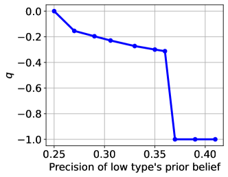
Figure 4: Results for Experiment G (Left) and H (Right). For both experiments, the vertical axis is the differential informativeness $q$ of the experiment used by $\theta_{L}$. For Experiment G (left), the horizontal axis is the frequency of the high type, and for Experiment H (right), the horizontal axis is the precision of the low type’s prior belief $\lvert\theta_{L}-0.5\rvert$.

The results are given in Figure 4. For Experiment C, increasing the high type’s frequency decreases the low type experiment’s informativeness. For Experiment D, increasing the precision of the low type’s prior belief decreases the low type experiment’s informativeness. Bergemann et al. (2018) characterize the informativeness of the optimal experiment for similar settings but for discrete distributions with two types. In particular, Proposition 3 from Bergemann et al. (2018) states that informativeness of the low type $\pi_{1,1}$, decreases when the frequency of the high type or with the precision of the low type’s prior belief $|\theta_{L}-0.5|$. It is interesting, then, that we observe the same behavior in the RochetNet results for a continuous analog of their discrete distribution set-up. This suggests a new target for economic theory.

5.2 Buyers with payoff and world prior heterogeneity

We are aware of no theoretical characterization of optimal data market designs when both $v$ and $\theta$ vary. In such cases, we can use RochetNet to conjecture the structure of an optimal solution. For this, we consider the following settings with enlarged buyer types (Setting D is parameterized by $c$):

1. Single buyer, Binary State, and Binary Actions, where the $v\sim U[0,1]$ and the interim beliefs are drawn from $U[0,1]$.

2. Single buyer, Binary State, and Binary Actions, where the $v\sim U[c,1]$ and the interim beliefs are drawn from an equal weight mixture of $\mathit{Beta}(8,30)$ and $\mathit{Beta}(60,30)$ for $c\in[0,1]$.

For Setting E, RochetNet learns a menu consisting of a single fully informative experiment with a price of $0.14$. For Setting F, RochetNet learns a menu consisting of a single fully informative experiment when $c<0.55$. For higher values of $c$, RochetNet learns an additional partially informative menu option. Further, in Figure 5, we show how the differential informativeness $q$ changes with $c$.

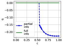
Figure 5: The differential informativeness $q$ of the menu(s) learned by RochetNet for Setting D, varying the parameter $c$ that instantiates the economic environment.

6 Experimental Results for the Multi-Buyer Setting

In this section, we show how we can use RegretNet to recover known existing results for the multi-buyer, BIC setting. We also use RegretNet to conjecture the optimal solution for a multi-buyer problem in the ex post IC setting and then prove the optimality of the design. Lastly, we give results for a setting where it is analytically hard to compute the optimal solution, but RegretNet is used to understand how revenue varies with changes to the intensity of negative externality, again building economic intuition for the market design problem.

6.1 BIC settings

Bonatti et al. (2022) study the multi-buyer market design problem with two buyers, binary actions, and fixed interim beliefs, the same for each agent. They show that a deterministic signaling scheme is optimal and thus characterize their solution in terms of recommending a correct action (selling a fully informative menu). Since the obedience constraints are defined on the interim representation, the optimal mechanism is also sometimes able to recommend incorrect actions to a buyer (in effect, sending recommendations that are opposed to the realized state).

We consider the settings studied by  Bonatti et al. (2022) and an additional setting:

1. The payoffs $v_{1},v_{2}$ are sampled from the exponential distribution with $\lambda=1$. The common and fixed interim beliefs are given by $\theta_{1}=\theta_{2}=(0.5,0.5)$. $\alpha$ is either 0.5 or 2.0

2. The payoffs $v_{1},v_{2}$ are sampled from the unit interval $U[0,1]$. The common and fixed interim beliefs are given by $\theta_{1}=\theta_{2}=(0.5,0.5)$. $\alpha$ is either 0.5 or 2.0

The results for these settings with a BIC constraint are shown in Figure 6. The theoretically optimum solution contains two kinds of recommendations, those recommending the correct action (the optimal action to take given the realized state) and those recommending incorrect actions, separated by the black solid lines. The heatmap shown in the plots denotes our computational results, which show the probability of recommending the correct action. In particular, we can confirm visually (and from its expected revenue) that RegretNet is able to recover the optimal revenue as well as the optimal experiment design. The test revenue and regret are given in Figure 7. We show additional results in Appendix G.1.

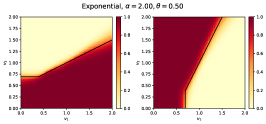
Figure 6: Experiments learned for Settings G (top) and H (bottom), for BIC constraints. The plot shows the probability of recommending the correct action to buyer $1$ (left subplot) and buyer $2$ (right subplot) for varying values of $v_{1}$ (x-axis) and $v_{2}$ (y-axis). For each setting, the theoretically optimal experiments are represented by solid lines separating the regions.

Setting	$\alpha$	RegretNet		Opt
		$\mathit{rev}$	$\mathit{rgt}$	$\mathit{rev}$
Setting G	0.5	0.632	$<0.001$	0.632
	2.0	1.603		1.613
Setting H	0.5	0.400	$<0.001$	0.396
	2.0	1.056		1.042

Figure 7: Test Revenue and Test Regret obtained by RegretNet for the Settings G and H, for BIC constraints.

Studying the effect of varying the intensity of externalities.

Following Bonatti et al. (2022), we can study the effect of the negative externality parameter $\alpha$ on the revenue for the BIC, multi-buyer setting with a common and known prior for each buyer and payoffs sampled from $U[0,1]$. We also consider the case where the payoffs are constant, but the interim beliefs are independently sampled from $U[0,1]$. While there is no known analytical characterization for the latter, we show how easy it is to study the models learned by RegretNet to analyze economic properties of interest.

Figure 8: Effect of $\alpha$ on revenue

Figure 8 shows the effect of $\alpha$ on the revenue. In the context of uncertain priors, we note that the effect on revenue is similar to the setting where payoffs are uncertain. As we enhance competition intensity via $\alpha$, the revenue grows. Even though the buyers are not recommended the correct action, the seller manages to generate revenue by threatening to share exclusive information with a competitor. This effect becomes fiercer in the settings with uncertain priors.

6.2 Ex post IC settings

We also apply RegretNet to the same settings (G and H), but while adopting ex post IC constraints. This is of interest because there is no known analytical solution for the optimal mechanism for two buyers in the ex post IC setting. The results are shown in Figure 9.

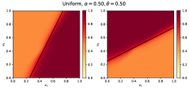
Figure 9: Experiments learned for Settings G (top) and H (bottom), for ex post IC constraints. The plot shows the probability of recommending the correct action to buyer $1$ (left subplot) and buyer $2$ (right subplot) for varying values of $v_{1}$ (x-axis) and $v_{2}$ (y-axis). For each setting, the conjectured optimal experiments are represented by solid lines separating the regions.

Based on this and additional experiments (in Appendix G.2), we were able to conjecture that the structure of the optimal design in this ex post IC setting, and we prove its optimality by following Myerson’s framework for single item auctions. We defer the proof to Appendix H.

Theorem 7.

Consider the setting with Binary State and Binary Actions where the buyers have a common interim belief $\theta_{i}=\theta$. The payoff $v_{i}$ for a buyer $i$ is drawn from a regular distribution $\mathcal{V}_{i}$ with a continuous density function. Define virtual value $\phi_{i}(v_{i})=v_{i}-\frac{1-F(v_{i})}{f(v_{i})}$, for pdf $f$ and cdf $F$ of distribution $\mathcal{V}_{i}$. The revenue-optimal mechanism satisfying ex post IC and IR is a mechanism that sells the fully informative experiment to buyer $i$ if $\phi_{i}(v_{i})\geq\frac{\alpha}{n-1}\sum_{i\not=j}\phi_{j}(v_{j})$. Otherwise, buyer $i$ receives an uninformative menu, where the signal corresponds to the most likely state based on the prior.

Distribution	$\alpha$	RegretNet		Opt
		$\mathit{rev}$	$\mathit{rgt}$	$\mathit{rev}$
Setting G	0.5	0.405	$<0.001$	0.405
	2.0	0.801		0.809
Setting H	0.5	0.277	$<0.001$	0.27
	2.0	0.553		0.541

Figure 10: Test Revenue and Test Regret obtained by RegretNet for the Settings G and H, for the ex post IC constraints. 

The exact test revenue and regret are given in Figure 10. We show additional results in Appendix G.2.

7 Conclusion

We have introduced a new deep neural network architecture and learning framework to study the design of optimal data markets. We have demonstrated through experimental work the flexibility of the framework, showing that it can adapt to relatively complex scenarios and facilitate the discovery of new optimal designs. Note that while we have only considered matching utility payoffs in this paper, our approach can easily be extended to non-matching utility payoffs as well.

We also point out some limitations. First, for our approach to continue to provide insights into the theoretically optimal design for larger problems (e.g., with more buyers, more signals, more actions), it will be important to provide interpretability to the mechanisms learned by RegretNet (designs learned by RochetNet, on the other hand, are immediately interpretable). Second, while our approach scales well with number of buyers, or states in the ex post IC setting, it does not scale as easily with the number of buyers in the BIC setting. The challenge in the BIC setting comes from the “interimf computations” involving conditional expectations over reports of others and scaling beyond what is studied in this paper will require new techniques, for example, exploiting symmetry. Third, we are making use of gradient-based approaches, which may suffer from local optima in non-convex problems. At the same time, deep learning has shown success in various problem domains despite non-convexity. The experiments reported here align with these observations, with our neural network architectures consistently recovering optimal solutions, when these are known and thus optimality can be verified, and despite non-convex formulations. Fourth, we attain in the multi-buyer setting only approximate, and not exact, incentive alignment, and this leaves the question of how much alignment is enough for agents to follow the intended advice of a market design (there is little practical or theoretical guidance in this regard). Moreover, we do not know for a given solution whether there is an exact IC solution nearby. While there is some recent guiding theory (Conitzer et al., 2022; Daskalakis and Weinberg, 2012; Cai et al., 2021) that provides transformations between $\epsilon$-BIC and BIC without revenue loss in the context of auction design, extending these transformations to approximate DSIC settings and problems with both types and actions presents an interesting avenue for future research.

Lastly, we return to where we started, and underline that markets for trading data about individuals raise substantive ethical concerns (Acemoglu et al. (2022); Acquisti et al. (2016); Athey et al. (2017); Bergemann et al. (2022a); Bonatti (2022); Choi et al. (2019); Fainmesser et al. (2022)). Our hope is that machine learning frameworks such as those introduced here can be used to strike new kinds of trade-offs, for example allowing individuals to also benefit directly from trades on data about themselves and to embrace privacy and fairness constraints.

Appendix A Setup and Hyper-parameters for the Single-Buyer Settings

Training.

We train RochetNet with $P=1000$ possible menu entries. We set the softmax temperature $\tau$ to $\frac{1}{200}$. We train RochetNet for $20,000$ iterations with a minibatch of size $2^{15}$ sampled online for every update.

Testing.

We report all our results on a test set of 20000 samples that are separate from the train set.

Training time.

For the settings studied in the paper, RochetNet takes 7-8 minutes to train on a single NVIDIA Tesla V100 GPU.

Appendix B Proof of Lemma 3

See 3

Proof.

For the ex post IC setting, we first compute a normalized payment, $\tilde{t}_{i}^{w}(\rho)\in[0,1]$, for each buyer $i$ by using a sigmoidal unit. We scale this by the difference between utility achieved by the buyer when he is truthful and obedient and the utility of opting out. Thus, the payment $t_{i}^{w}(\rho)$ is computed as follows:

$$t_{i}^{w}(\rho)=\tilde{t}_{i}^{w}(\rho)\cdot v_{i}\cdot\left(\sum_{k\in[m]}\pi_{i,k,k}^{w}(\rho)\theta_{i,k}-\bar{\alpha}\sum_{k\in[m]}\sum_{j\in[n]\setminus i}\pi_{j,k,k}^{w}(\rho)\theta_{j,k}-(\max_{k}\theta_{i,k}-\alpha)\right)$$ (20)

To establish ex post IR, we reason about the utility a buyer can obtain when not participating in the mechanism. As per the discussion in Section 2.3, in an optimal data market the seller will send optimal recommendations to participating buyers in the event that buyer $i$ opts out, thus minimizing the utility of the buyer who opts out. In particular, the recommendation for any $j\neq i$, for an opting out buyer $i$, is such that $\mathop{\mathbb{E}}_{\begin{subarray}{c}a\sim\sigma_{-i}(\omega;\rho_{-i})\\ \omega\sim\theta_{i}\end{subarray}}\left[\mathbf{1}\{a_{j}=\omega\}\right]=1$. Given this, the utility of buyer $i$, when opting out, is

$$\min_{\sigma_{-i}}\max_{\tilde{a}_{i}\in\mathcal{A}_{i}} \left(\mathop{\mathbb{E}}_{\begin{subarray}{c}a\sim\sigma_{-i}(\omega;\rho_{-i}),\\ \omega\sim\theta_{i}\end{subarray}}\left[u_{i}(\tilde{a}_{i},a_{-i};\omega,\rho)\right]\right)$$ (21)

$$=\max_{\tilde{a}_{i}\in\mathcal{A}_{i}}\left(\mathbb{E}_{\begin{subarray}{c}a\sim\sigma_{-i}(\omega;\rho_{-i})\\ \omega\sim\theta_{i}\end{subarray}}\left[v_{i}\cdot\mathbf{1}\{\tilde{a}_{i}=\omega\}-v_{i}\bar{\alpha}\sum_{j\in[n]\setminus i}\mathbf{1}\{\tilde{a}_{i}=\omega\}\right]\right)$$

$$=\max_{\tilde{a}_{i}\in\mathcal{A}_{i}}\left(\mathbb{E}_{\omega\sim\theta_{i}}\left[v_{i}\cdot\mathbf{1}\{\tilde{a}_{i}=\omega\}-v_{i}\alpha\right]\right)$$

$$=v_{i}\cdot\left(\max\theta_{i}-\alpha\right).$$

Note that $\sum_{k\in[m]}\pi_{i,k,k}^{w}(\rho)\theta_{i,k}\geq\max_{k}\theta_{i,k}$ and $\bar{\alpha}\left(\sum_{k\in[m]}\sum_{j\in[n]\setminus i}\pi_{j,k,k}^{w}(\rho)\theta_{j,k}\right)\leq\bar{\alpha}\left(\sum_{j\in[n]\setminus i}1\right)=\alpha$. Thus we have $\sum_{k\in[m]}\pi_{i,k,k}^{w}(\rho)\theta_{i,k}-\bar{\alpha}\left(\sum_{k\in[m]}\sum_{j\in[n]\setminus i}\pi_{j,k,k}^{w}(\rho)\theta_{j,k}\right)-\left(\max_{k}\theta_{i,k}-\alpha\right)\geq 0$.

Taking this with the fact that $\tilde{t}_{i}^{w}(\rho)\in[0,1]$, we have

$$t^{w}_{i}(\rho) =\tilde{t}_{i}^{w}(\rho)\cdot v_{i}\cdot\left(\sum_{k\in[m]}\pi_{i,k,k}^{w}(\rho)\theta_{i,k}-\bar{\alpha}\sum_{k\in[m]}\sum_{j\in[n]\setminus i}\pi_{j,k,k}^{w}(\rho)\theta_{j,k}-(\max_{k}\theta_{i,k}-\alpha)\right)$$ (22)

$$\leq v_{i}\cdot\left(\mathop{\mathbb{E}}_{\begin{subarray}{c}a\sim\sigma_{i}^{w}(\omega;\rho),\\ \omega\sim\theta_{i}\end{subarray}}\left[\left(\mathbf{1}\{a_{i}=\omega\}-\bar{\alpha}\sum_{j\in[n]\setminus i}\mathbf{1}\{a_{j}=\omega\}\right)\right]-\left(\max_{k}\theta_{i,k}-\alpha)\right)\right)$$

$$=\mathop{\mathbb{E}}_{\begin{subarray}{c}a\sim\sigma_{i}^{w}(\omega;\rho),\\ \omega\sim\theta_{i}\end{subarray}}\left[v_{i}\cdot\left(\mathbf{1}\{a_{i}=\omega\}-\bar{\alpha}\sum_{j\in[n]\setminus i}\mathbf{1}\{a_{j}=\omega\}\right)\right]-v_{i}\cdot\left(\max_{k}\theta_{i,k}-\alpha)\right)$$

$$=\mathop{\mathbb{E}}_{\begin{subarray}{c}a\sim\sigma_{i}^{w}(\omega;\rho),\\ \omega\sim\theta_{i}\end{subarray}}\left[u_{i}(a;\omega,\rho)\right]-v_{i}\cdot\left(\max\theta_{i}-\alpha)\right)$$

Rearranging, and substituting $v_{i}\cdot\left(\max\theta_{i}-\alpha\right)$ from Eqn 21, we get the IR constraint described in Eqn 9. ∎

Appendix C Proof of Lemma 4

See 4

Proof.

For the BIC setting, we work with the interim payment, and make use of a normalized interim payment, $\tilde{t}_{i}(\rho_{i})\in[0,1]$, for each buyer $i$, by using a sigmoidal unit. In this case, we scale this normalized payment by the difference between the interim utility achieved when the buyer is truthful and obedient and the interim utility of opting out. Thus, the interim payment is

$$t_{i}^{w}(\rho_{i})=\tilde{t}_{i}^{w}(\rho_{i})\cdot v_{i}\cdot\hat{\mathbb{E}}_{-i}\left[\sum_{k\in[m]}\pi_{i,k,k}^{w}(\rho)\theta_{i,k}-\bar{\alpha}\sum_{k\in[m]}\sum_{j\in[n]\setminus i}\pi_{j,k,k}^{w}(\rho)\theta_{j,k}-(\max\theta_{i}-\alpha)\right]$$ (23)

The utility of the outside option is again computed similarly to the ex post IC setting, recognizing that the seller in the optimal mechanism will make optimal recommendation to participating buyers in the event that buyer $i$ opts out. In particular, $\hat{\mathbb{E}}_{-i}\left[\mathop{\mathbb{E}}_{\begin{subarray}{c}a\sim\sigma_{-i}(\omega;\rho_{-i}),\\ \omega\sim\theta_{i}\end{subarray}}\left[\mathbf{1}\{a_{j}=\omega\}\right]\right]=1$ to any agent $j\not=i$, in such as case. In particular, the utility of buyer $i$, when opting out, is

$$\min_{\sigma_{-i}}\max_{\tilde{a}_{i}\in\mathcal{A}_{i}} \left(\hat{\mathbb{E}}_{-i}\left[\mathop{\mathbb{E}}_{\begin{subarray}{c}a\sim\sigma_{-i}(\omega;\rho_{-i}),\\ \omega\sim\theta_{i}\end{subarray}}\left[u_{i}(\tilde{a}_{i},a_{-i};\omega,\rho)\right]\right]\right)$$ (24)

$$=\max_{\tilde{a}_{i}\in\mathcal{A}_{i}}\left(\hat{\mathbb{E}}_{-i}\left[\mathbb{E}_{\begin{subarray}{c}a\sim\sigma_{-i}(\omega;\rho_{-i}),\\ \omega\sim\theta_{i}\end{subarray}}\left[v_{i}\cdot\mathbf{1}\{\tilde{a}_{i}=\omega\}-v_{i}\bar{\alpha}\sum_{j\in[n]\setminus i}\mathbf{1}\{a_{j}=\omega\}\right]\right]\right)$$

$$=\max_{\tilde{a}_{i}\in\mathcal{A}_{i}}\left(\mathbb{E}_{\omega\sim\theta_{i}}\left[v_{i}\cdot\mathbf{1}\{\tilde{a}_{i}=\omega\}-v_{i}\alpha\right]\right)$$

$$=v_{i}\cdot\left(\max\theta_{i}-\alpha\right)$$

Note that $\hat{\mathbb{E}}_{-i}\left[\sum_{k\in[m]}\pi_{i,k,k}^{w}(\rho)\theta_{i,k}\right]\geq\max_{k}\theta_{i,k}$ and $\hat{\mathbb{E}}_{-i}\left[\bar{\alpha}\left(\sum_{k\in[m]}\sum_{j\in[n]\setminus i}\pi_{j,k,k}^{w}(\rho)\theta_{j,k}\right)\right]\leq\bar{\alpha}\left(\sum_{j\in[n]\setminus i}1\right)=\alpha$. Thus we have:

$$\hat{\mathbb{E}}_{-i}\left[\sum_{k\in[m]}\pi_{i,k,k}^{w}(\rho)\theta_{i,k}-\bar{\alpha}\sum_{k\in[m]}\sum_{j\in[n]\setminus i}\pi_{j,k,k}^{w}(\rho)\theta_{j,k}-\left(\max_{k}\theta_{i,k}-\alpha\right)\right]\geq 0$$

Taking this with the fact that $\tilde{t}_{i}^{w}(\rho_{i})\in[0,1]$, we have

$$t_{i}^{w}(\rho_{i}) =\tilde{t}_{i}^{w}(\rho_{i})\cdot v_{i}\cdot\hat{\mathbb{E}}_{-i}\left[\sum_{k\in[m]}\pi_{i,k,k}^{w}(\rho)\theta_{i,k}-\bar{\alpha}\sum_{k\in[m]}\sum_{j\in[n]\setminus i}\pi_{j,k,k}^{w}(\rho)\theta_{j,k}-(\max\theta_{i}-\alpha)\right]$$ (25)

$$\leq v_{i}\cdot\hat{\mathbb{E}}_{-i}\left[\sum_{k\in[m]}\pi_{i,k,k}^{w}(\rho)\theta_{i,k}-\bar{\alpha}\sum_{k\in[m]}\sum_{j\in[n]\setminus i}\pi_{j,k,k}^{w}(\rho)\theta_{j,k}\right]-v_{i}\cdot\left(\max\theta_{i}-\alpha)\right)$$

$$=\hat{\mathbb{E}}_{-i}\left[\mathop{\mathbb{E}}_{\begin{subarray}{c}a\sim\sigma_{i}^{w}(\omega;\rho),\\ \omega\sim\theta_{i}\end{subarray}}\left[v_{i}\cdot\left(\mathbf{1}\{a_{i}=\omega\}-\bar{\alpha}\sum_{j\in[n]\setminus i}\mathbf{1}\{a_{j}=\omega\}\right)\right]\right]-v_{i}\cdot\left(\max\theta_{i}-\alpha)\right)$$

$$\leq\hat{\mathbb{E}}_{-i}\left[\mathop{\mathbb{E}}_{\begin{subarray}{c}a\sim\sigma_{i}^{w}(\omega;\rho),\\ \omega\sim\theta_{i}\end{subarray}}\left[u_{i}(a;\omega,\rho)\right]\right]-v_{i}\cdot\left(\max\theta_{i}-\alpha)\right)$$

Rearranging the above and substituting $v_{i}\cdot\left(\max\theta_{i}-\alpha\right)$ from Eqn 24, we get the IIR constraint described in Eqn 8.

∎

Appendix D Proof of Lemma 5

See 5

Proof.

We first prove the forward direction: if any mechanism $\mathcal{M}=\left(\sigma^{w},t^{w}\right)$ where $\sigma_{i}^{w}(\omega,\rho)=\left(\pi_{i,\omega}^{w}(\rho)\right)$ is ex post IC, then $RGT_{i}^{w}=0,\forall i\in[n]$.

For the ex post IC setting, the incentive compatibility constraints requires that for every agent $i$, and for each $\rho\in\mathcal{P}$, and assuming that every other agent reports its type truthfully and follows the recommended action, then for each misreport $\rho_{i}^{\prime}\in\mathcal{P}_{i}$, and each deviation function, $\delta:\mathcal{A}_{i}\to\mathcal{A}_{i}$, the following condition:

$$\mathop{\mathbb{E}}_{\begin{subarray}{c}a\sim\sigma(\omega,\rho),\\ \omega\sim\theta_{i}\end{subarray}}\left[u_{i}(a,\omega,\rho)-t_{i}(\rho)\right]\geq\mathop{\mathbb{E}}_{\begin{subarray}{c}a\sim\sigma(\omega;\rho_{i}^{\prime},\rho_{-i}),\\ \omega\sim\theta_{i}\end{subarray}\ }\left[u_{i}(\delta(a_{i}),a_{-i},\omega,\rho)-t_{i}(\rho_{i}^{\prime},\rho_{-i})\right]$$ (26)

Note that the above hold for any deviation function $\delta$. Therefore, we can write that

$$\mathop{\mathbb{E}}_{\begin{subarray}{c}a\sim\sigma(\omega,\rho),\\ \omega\sim\theta_{i}\end{subarray}}\left[u_{i}(a,\omega,\rho)-t_{i}(\rho)\right]\geq\max_{\delta}\mathop{\mathbb{E}}_{\begin{subarray}{c}a\sim\sigma(\omega;\rho_{i}^{\prime},\rho_{-i}),\\ \omega\sim\theta_{i}\end{subarray}\ }\left[u_{i}(\delta(a_{i}),a_{-i},\omega,\rho)-t_{i}(\rho_{i}^{\prime},\rho_{-i})\right]$$ (27)

We can expand to get the following equation:

$$v_{i}\cdot\left(\sum_{k\in[m]}\pi_{i,k,k}^{w}(\rho)\theta_{i,k}-\bar{\alpha}\sum_{k\in[m]}\sum_{j\in[n]\setminus i}\pi_{j,k,k}^{w}(\rho)\theta_{j,k}\right)-t_{i}(\rho)\\ \geq\max_{\delta}v_{i}\cdot\left(\sum_{k\in[m]}\left\{\pi_{i,\delta(k),k}^{w}(\rho^{\prime}_{i},\rho_{-i})\theta_{i,\delta(k)}\right\}-\bar{\alpha}\sum_{k\in[m]}\sum_{j\in[n]\setminus i}\pi_{j,k,k}^{w}(\rho^{\prime}_{i},\rho_{-i})\theta_{j,k}\right)-t_{i}(\rho^{\prime}_{i},\rho_{-i})$$ (28)

Pushing the max inside (since other terms don’t involve $\delta(k)$), we note that:

$$\max_{\delta}\sum_{k\in[m]}\left\{\pi_{i,\delta(k),k}^{w}(\rho^{\prime}_{i},\rho_{-i})\theta_{i,\delta(k)}\right\}=\sum_{k\in[m]}\max_{k^{\prime}}\left\{\pi_{i,k^{\prime},k}^{w}(\rho^{\prime}_{i},\rho_{-i})\theta_{i,k^{\prime}}\right\}$$ (29)

Thus we have,

$$v_{i}\cdot\left(\sum_{k\in[m]}\pi_{i,k,k}^{w}(\rho)\theta_{i,k}-\bar{\alpha}\sum_{k\in[m]}\sum_{j\in[n]\setminus i}\pi_{j,k,k}^{w}(\rho)\theta_{j,k}\right)-t_{i}(\rho)\\ \geq v_{i}\cdot\left(\sum_{k\in[m]}\max_{k^{\prime}\in[m]}\left\{\pi_{i,k^{\prime},k}^{w}(\rho^{\prime}_{i},\rho_{-i})\theta_{i,k^{\prime}}\right\}-\bar{\alpha}\sum_{k\in[m]}\sum_{j\in[n]\setminus i}\pi_{j,k,k}^{w}(\rho^{\prime}_{i},\rho_{-i})\theta_{j,k}\right)-t_{i}(\rho^{\prime}_{i},\rho_{-i})$$ (30)

Note that by our definition of ex post regret in Equation 18, the above is equivalent to $rgt^{w}_{i}(\rho^{\prime}_{i},\rho)\leq 0$. Furthermore, this holds for any deviating report $\rho_{i}^{\prime}$. Thus, we can write:

$$\max_{\rho^{\prime}_{i}\in\mathcal{P}_{i}}rgt^{w}_{i}(\rho^{\prime}_{i},\rho)\leq 0$$ (31)

But note that

$$\begin{split}\max_{\rho_{i}^{\prime}\in\mathcal{P}_{i}}rgt_{i}^{w}\left(\rho_{i}^{\prime},\rho\right)&\geq rgt_{i}^{w}\left(\rho_{i},\rho\right)\\ &=v_{i}\cdot\left(\sum_{k\in[m]}\max_{k^{\prime}\in[m]}\left\{\pi_{i,k^{\prime},k}^{w}(\rho)\theta_{i,k^{\prime}}\right\}-\bar{\alpha}\sum_{k\in[m]}\sum_{j\in[n]\setminus i}\pi_{j,k,k}^{w}(\rho)\theta_{j,k}\right)\\ &\qquad-v_{i}\cdot\left(\sum_{k\in[m]}\pi_{i,k,k}^{w}(\rho)\theta_{i,k}-\bar{\alpha}\sum_{k\in[m]}\sum_{j\in[n]\setminus i}\pi_{j,k,k}^{w}(\rho)\theta_{j,k}\right)\\ &=v_{i}\cdot\left(\sum_{k\in[m]}\left[\max_{k^{\prime}\in[m]}\left\{\pi_{i,k^{\prime},k}^{w}(\rho)\theta_{i,k^{\prime}}\right\}-\pi_{i,k,k}^{w}(\rho)\theta_{i,k}\right]\right)\\ &\geq 0\end{split}$$ (32)

where the last step holds since $\max_{k^{\prime}\in[m]}\left\{\pi_{i,k^{\prime},k}^{w}(\rho)\theta_{i,k^{\prime}}\right\}\geq\pi_{i,k,k}^{w}(\rho)\theta_{i,k}$

Combining Equations 31 and 32, we have $\max_{\rho^{\prime}_{i}\in\mathcal{P}_{i}}rgt^{w}_{i}(\rho^{\prime}_{i},\rho)=0$. Taking the expectation over all profiles $\rho\in\mathcal{P}$, we have $\mathbb{E}_{\rho\in\mathcal{P}}\left[\max_{\rho_{i}^{\prime}\in\mathcal{P}_{i}}rgt_{i}^{w}\left(\rho_{i}^{\prime},\rho\right)\right]=0$. Thus, $RGT_{i}^{w}=0,\forall i\in[n]$. Thus, we’ve shown that if any mechanism $\mathcal{M}=\left(\sigma^{w},t^{w}\right)$ where $\sigma_{i}^{w}(\omega,\rho)=\left(\pi_{i,\omega}^{w}(\rho)\right)$ is ex post IC, then $RGT_{i}^{w}=0$, as desired.

Next, we consider the reverse direction: if $RGT_{i}^{w}=0,\forall i\in[n]$, we want to show that any mechanism $\mathcal{M}=\left(\sigma^{w},t^{w}\right)$ where $\sigma_{i}^{w}(\omega,\rho)=\left(\pi_{i,\omega}^{w}(\rho)\right)$ is ex post IC. Starting with $RGT_{i}^{w}=0,\forall i\in[n]$, we have that by definition: $\mathbb{E}_{\rho\in\mathcal{P}}\left[\max_{\rho_{i}^{\prime}\in\mathcal{P}_{i}}rgt_{i}^{w}\left(\rho_{i}^{\prime},\rho\right)\right]=0$. But we showed in Equation 32 that $\max_{\rho_{i}^{\prime}\in\mathcal{P}_{i}}rgt_{i}^{w}\left(\rho_{i}^{\prime},\rho\right)\geq 0$. Thus we have that $\max_{\rho_{i}^{\prime}\in\mathcal{P}_{i}}rgt_{i}^{w}\left(\rho_{i}^{\prime},\rho\right)=0\implies rgt_{i}^{w}\left(\rho_{i}^{\prime},\rho\right)\leq 0$.

Plugging in our definition for ex post regret, we have that:

$$v_{i}\cdot\left(\sum_{k\in[m]}\max_{k^{\prime}\in[m]}\left\{\pi_{i,k^{\prime},k}^{w}(\rho^{\prime}_{i},\rho_{-i})\theta_{i,k^{\prime}}\right\}-\bar{\alpha}\sum_{k\in[m]}\sum_{j\in[n]\setminus i}\pi_{j,k,k}^{w}(\rho^{\prime}_{i},\rho_{-i})\theta_{j,k}\right)\\ -v_{i}\cdot\left(\sum_{k\in[m]}\pi_{i,k,k}^{w}(\rho)\theta_{i,k}-\bar{\alpha}\sum_{k\in[m]}\sum_{j\in[n]\setminus i}\pi_{j,k,k}^{w}(\rho)\theta_{j,k}\right)-\left(t^{w}_{i}(\rho^{\prime}_{i},\rho_{-i})-t^{w}_{i}(\rho)\right)\leq 0$$ (33)

This can be transformed back to:

$$\mathop{\mathbb{E}}_{\begin{subarray}{c}a\sim\sigma(\omega,\rho)\\ \omega\sim\theta_{i}\end{subarray}}\left[u_{i}(a,\omega,\rho)-t_{i}(\rho)\right] \geq\max_{\delta}\mathop{\mathbb{E}}_{\begin{subarray}{c}a\sim\sigma(\omega;\rho_{i}^{\prime},\rho_{-i}),\\ \omega\sim\theta_{i}\end{subarray}\ }\left[u_{i}(\delta(a_{i}),a_{-i},\omega,\rho)-t_{i}(\rho_{i}^{\prime},\rho_{-i})\right]$$ (34)

$$\geq\mathop{\mathbb{E}}_{\begin{subarray}{c}a\sim\sigma(\omega;\rho_{i}^{\prime},\rho_{-i})\\ \omega\sim\theta_{i}\end{subarray}\ }\left[u_{i}(\delta(a_{i}),a_{-i},\omega,\rho)-t_{i}(\rho_{i}^{\prime},\rho_{-i})\right]$$

This is exactly the ex post IC constraint described in Equation 4

∎

Appendix E Proof of Lemma 6

See 6

Proof.

We first prove the forward direction: if any mechanism $\mathcal{M}=\left(\sigma^{w},t^{w}\right)$ where $\sigma_{i}^{w}(\omega,\rho)=\left(\pi_{i,\omega}^{w}(\rho)\right)$ is interim IC, then $\widehat{RGT}_{i}^{w}=0,\forall i\in[n]$.

For the BIC setting, for each $(\rho_{i},\rho_{i}^{\prime})\in\mathcal{P}_{i}^{2}$ and for each deviation function $\delta:\mathcal{A}_{i}\to\mathcal{A}_{i}$, a BIC mechanism satisfies:

$$\hat{\mathbb{E}}_{-i}\left[\mathop{\mathbb{E}}_{\begin{subarray}{c}a\sim\sigma(\omega,\rho)\\ \omega\sim\theta_{i}\end{subarray}}\left[u_{i}(a,\omega,\rho)-t_{i}(\rho)\right]\right]\geq\hat{\mathbb{E}}_{-i}\left[\mathop{\mathbb{E}}_{\begin{subarray}{c}a\sim\sigma(\omega;\rho_{i}^{\prime},\rho_{-i})\\ \omega\sim\theta_{i}\end{subarray}}\left[u_{i}(\delta(a_{i}),a_{-i},\omega,\rho)-t_{i}(\rho_{i}^{\prime},\rho_{-i})\right]\right]$$ (35)

Note that the above hold for any deviation function $\delta$, therefore we can write that

$$\hat{\mathbb{E}}_{-i}\left[\mathop{\mathbb{E}}_{\begin{subarray}{c}a\sim\sigma(\omega,\rho)\\ \omega\sim\theta_{i}\end{subarray}}\left[u_{i}(a,\omega,\rho)-t_{i}(\rho)\right]\right]\geq\max_{\delta}\hat{\mathbb{E}}_{-i}\left[\mathop{\mathbb{E}}_{\begin{subarray}{c}a\sim\sigma(\omega;\rho_{i}^{\prime},\rho_{-i})\\ \omega\sim\theta_{i}\end{subarray}}\left[u_{i}(\delta(a_{i}),a_{-i},\omega,\rho)-t_{i}(\rho_{i}^{\prime},\rho_{-i})\right]\right]$$ (36)

We can expand to get the following equations:

$$v_{i} \cdot\hat{\mathbb{E}}_{-i}\left[\sum_{k\in[m]}\pi_{i,k,k}^{w}(\rho_{i},\rho_{-i})\theta_{i,k}-\bar{\alpha}\sum_{k\in[m]}\sum_{j\in[n]\setminus i}\pi_{j,k,k}^{w}(\rho_{i},\rho_{-i})\theta_{j,k}\right]-t_{i}(\rho_{i})$$ (37)

$$\geq\max_{\delta}v_{i}\cdot\hat{\mathbb{E}}_{-i}\left[\left(\sum_{k\in[m]}\pi_{i,\delta(k),k}^{w}(\rho^{\prime}_{i},\rho_{-i})\theta_{i,\delta(k)}-\bar{\alpha}\sum_{k\in[m]}\sum_{j\in[n]\setminus i}\pi_{j,k,k}^{w}(\rho^{\prime}_{i},\rho_{-i})\theta_{j,k}\right)\right]-t_{i}(\rho^{\prime}_{i})$$

$$=\max_{\delta}v_{i}\cdot\left(\sum_{k\in[m]}\hat{\mathbb{E}}_{-i}\left[\pi_{i,\delta(k),k}^{w}(\rho^{\prime}_{i},\rho_{-i})\theta_{i,\delta(k)}-\bar{\alpha}\sum_{j\in[n]\setminus i}\pi_{j,k,k}^{w}(\rho^{\prime}_{i},\rho_{-i})\theta_{j,k}\right]\right)-t_{i}(\rho^{\prime}_{i})$$

$$=v_{i}\cdot\left(\sum_{k\in[m]}\max_{\delta}\hat{\mathbb{E}}_{-i}\left[\pi_{i,\delta(k),k}^{w}(\rho^{\prime}_{i},\rho_{-i})\theta_{i,\delta(k)}-\bar{\alpha}\sum_{j\in[n]\setminus i}\pi_{j,k,k}^{w}(\rho^{\prime}_{i},\rho_{-i})\theta_{j,k}\right]\right)-t_{i}(\rho^{\prime}_{i})$$

$$=v_{i}\cdot\left(\sum_{k\in[m]}\max_{k^{\prime}\in[m]}\hat{\mathbb{E}}_{-i}\left[\pi_{i,k^{\prime},k}^{w}(\rho^{\prime}_{i},\rho_{-i})\theta_{i,\delta(k)}-\bar{\alpha}\sum_{j\in[n]\setminus i}\pi_{j,k,k}^{w}(\rho^{\prime}_{i},\rho_{-i})\theta_{j,k}\right]\right)-t_{i}(\rho^{\prime}_{i})$$

The above equations follow from the linearity of expectations and from pushing the max to the inside (since other terms don’t involve $\delta(k)$).

Note that by our definition of interim regret in Equation 19, the above equation is equivalent to $\widehat{rgt}_{i}^{w}\left(\rho_{i}^{\prime},\rho_{i}\right)\leq 0$. Furthermore, this holds for any deviating report $\rho^{\prime}_{i}$. Therefore, we can write that

$$\max_{\rho^{\prime}_{i}\in\mathcal{P}_{i}}\widehat{rgt}^{w}_{i}(\rho^{\prime}_{i},\rho_{i})\leq 0$$ (38)

But note that

$$\begin{split}\max_{\rho_{i}^{\prime}\in\mathcal{P}_{i}}\widehat{rgt}_{i}^{w}\left(\rho_{i}^{\prime},\rho\right)&\geq\widehat{rgt}^{w}_{i}(\rho_{i},\rho_{i})\\ &=v_{i}\cdot\left(\sum_{k\in[m]}\max_{k^{\prime}\in[m]}\hat{\mathbb{E}}_{-i}\left[\pi_{i,k^{\prime},k}^{w}(\rho_{i},\rho_{-i})\theta_{i,k^{\prime}}-\bar{\alpha}\sum_{j\in[n]\setminus i}\pi_{j,k,k}^{w}(\rho_{i},\rho_{-i})\theta_{j,k}\right]\right)-t_{i}(\rho_{i})\\ &\qquad-v_{i}\cdot\hat{\mathbb{E}}_{-i}\left[\sum_{k\in[m]}\pi_{i,k,k}^{w}(\rho_{i},\rho_{-i})\theta_{i,k}-\bar{\alpha}\sum_{k\in[m]}\sum_{j\in[n]\setminus i}\pi_{j,k,k}^{w}(\rho_{i},\rho_{-i})\theta_{j,k}\right]+t_{i}(\rho_{i})\\ &=v_{i}\cdot\left(\sum_{k\in[m]}\max_{k^{\prime}\in[m]}\hat{\mathbb{E}}_{-i}\left[\pi_{i,k^{\prime},k}^{w}(\rho_{i},\rho_{-i})\theta_{i,k^{\prime}}\right]-\hat{\mathbb{E}}_{-i}\left[\pi_{i,k,k}^{w}(\rho_{i},\rho_{-i})\theta_{i,k}\right]\right)\\ &\geq 0\end{split}$$ (39)

where the second step follows from linearity of expectation, and the last step holds since we are taking the max of all possible $k^{\prime}\in[m]$, which includes $k^{\prime}=k$.

Combining Equations 38 and 39, we have that $\max_{\rho^{\prime}_{i}\in\mathcal{P}_{i}}\widehat{rgt}^{w}_{i}(\rho^{\prime}_{i},\rho_{i})=0$. Taking the expectation over all profiles $\rho$, we have $\hat{\mathbb{E}}_{\rho\in\mathcal{P}}\left[\max_{\rho_{i}^{\prime}\in\mathcal{P}_{i}}\widehat{rgt}_{i}^{w}\left(\rho_{i}^{\prime},\rho_{i}\right)\right]=0\implies\widehat{RGT}_{i}^{w}=0,\forall i\in[n]$. Thus, we’ve showed that if any mechanism $\mathcal{M}=\left(\sigma^{w},t^{w}\right)$ where $\sigma_{i}^{w}(\omega,\rho)=\left(\pi_{i,\omega}^{w}(\rho)\right)$ is BIC, then $\widehat{RGT}_{i}^{w}=0$, as desired.

Next, we consider the reverse direction: if $\widehat{RGT}_{i}^{w}=0,\forall i\in[n]$, we want to show that any mechanism $\mathcal{M}=\left(\sigma^{w},t^{w}\right)$ where $\sigma_{i}^{w}(\omega,\rho)=\left(\pi_{i,\omega}^{w}(\rho)\right)$ is BIC. Starting with $\widehat{RGT}_{i}^{w}=0,\forall i\in[n]$, we have that by definition: $\hat{\mathbb{E}}_{\rho\in\mathcal{P}}\left[\max_{\rho_{i}^{\prime}\in\mathcal{P}_{i}}\widehat{rgt}_{i}^{w}\left(\rho^{\prime}_{i},\rho_{i}\right)\right]=0$. But we showed in Equation 39 that $\max_{\rho_{i}^{\prime}\in\mathcal{P}_{i}}\widehat{rgt}_{i}^{w}\left(\rho_{i}^{\prime},\rho_{i}\right)\geq 0$. Thus we have $\max_{\rho_{i}^{\prime}\in\mathcal{P}_{i}}\widehat{rgt}_{i}^{w}\left(\rho_{i}^{\prime},\rho_{i}\right)=0\implies\widehat{rgt}_{i}^{w}\left(\rho_{i}^{\prime},\rho_{i}\right)\leq 0$. Plugging in our definition for interim regret, we have that:

$$v_{i}\cdot\left(\sum_{k\in[m]}\max_{k^{\prime}\in[m]}\hat{\mathbb{E}}_{-i}\left[\pi_{i,k^{\prime},k}^{w}(\rho^{\prime}_{i},\rho_{-i})\theta_{i,k^{\prime}}-\bar{\alpha}\sum_{j\in[n]\setminus i}\pi_{j,k,k}^{w}(\rho^{\prime}_{i},\rho_{-i})\theta_{j,k}\right]\right)-t_{i}(\rho^{\prime}_{i})\\ \leq v_{i}\cdot\hat{\mathbb{E}}_{-i}\left[\sum_{k\in[m]}\pi_{i,k,k}^{w}(\rho_{i},\rho_{-i})\theta_{i,k}-\bar{\alpha}\sum_{k\in[m]}\sum_{j\in[n]\setminus i}\pi_{j,k,k}^{w}(\rho_{i},\rho_{-i})\theta_{j,k}\right]-t_{i}(\rho_{i})$$ (40)

This can be transformed back to:

$$\hat{\mathbb{E}}_{-i}\left[\mathop{\mathbb{E}}_{\begin{subarray}{c}a\sim\sigma(\omega,\rho)\\ \omega\sim\theta_{i}\end{subarray}}\left[u_{i}(a,\omega,\rho)-t_{i}(\rho)\right]\right] \geq\max_{\delta}\hat{\mathbb{E}}_{-i}\left[\mathop{\mathbb{E}}_{\begin{subarray}{c}a\sim\sigma(\omega;\rho_{i}^{\prime},\rho_{-i})\\ \omega\sim\theta_{i}\end{subarray}}\left[u_{i}(\delta(a_{i}),a_{-i},\omega,\rho)-t_{i}(\rho_{i}^{\prime},\rho_{-i})\right]\right]$$ (41)

$$\geq\hat{\mathbb{E}}_{-i}\left[\mathop{\mathbb{E}}_{\begin{subarray}{c}a\sim\sigma(\omega;\rho_{i}^{\prime},\rho_{-i})\\ \omega\sim\theta_{i}\end{subarray}}\left[u_{i}(\delta(a_{i}),a_{-i},\omega,\rho)-t_{i}(\rho_{i}^{\prime},\rho_{-i})\right]\right]$$

This is exactly the interim IC constraint described in Equation 1

∎

Appendix F Setup and Hyper-parameters for the Multi-Buyer Settings

Training.

For the multi-buyer setting, all our neural networks consist of $3$ hidden layers with $200$ hidden units each. For the IC setting, we sample a minibatch of $1024$ samples online to update the parameters of the neural networks. We sample $100$ misreports for every sample to compute the best initialization. For the BIC setting, we use a minibatch of $128$ samples. We compute the interim values wherever required over $512$ samples drawn from $\mathcal{P}_{-i}$.

We observe that sampling alone is sufficient to approximate the regret while training and do not perform any additional gradient descent steps, as this does not improve the training performance (however, we anticipate this step would be necessary for larger settings).

We train the neural networks for $20,000$ iterations and make parameter updates using the Adam Optimizer with a learning rate of $0.001$. The Lagrangian parameters $(\lambda_{1},\ldots\lambda_{n})$ are set to $10.0$. The coefficient of the penalty term is initialized to $1.0$. The Lagrangian updates are performed once every $100$ iterations.

Testing.

We report all our results on a test size of $20000$ samples. For the DSIC setting, we use 100 misreports as initialization to warm-start the inner maximization to compute regret. For the BIC setting, we use other samples of the minibatch to compute a defeating misreport as noted in the previous subsection. We then run $100$ steps of gradient ascent with a learning rate of $0.005$ to compute the defeating misreport and the regret more accurately.

Training time.

RegretNet takes 11 - 12 minutes per experiment for training for all the settings studied in this paper. All our experiments were run on a single NVIDIA Tesla V100 GPU.

Appendix G Additional Experimental Results for the Multi-Buyer Setting

We consider the following multi-buyer data market design problem with two buyers, binary action, and fixed interim beliefs, adopting all possible combinations of the following choices in regard to the configuration of the economy:

• $\theta=(0.5,0.5)$ or $\theta=(0.75,0.25)$

• $\alpha=0.5$ or $\alpha=2.0$

• Both payoffs are drawn from UNF, EXP, or Asym UNF

UNF is the uniform distribution over the unit interval $U[0,1]$. EXP is the exponential distribution with $\lambda=1$. For the Asym UNF, the payoff for buyer $i$ is uniform over the interval $[0,i+1]$. In the next two subsections, we present our results for the BIC and ex post IC settings, respectively.

G.1 BIC Settings

Figures 11, 12, and 13 show the optimal data market design and the data marker learned by RegretNet for the BIC settings described above, and Figure 14 gives the test revenue and regret obtained by RegretNet and the revenue of the optimal mechanism.

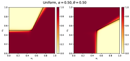
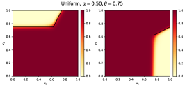
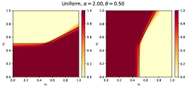
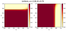
Figure 11: Experiments learned for BIC constraints when the payoffs are drawn from UNF

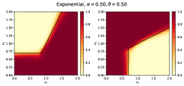
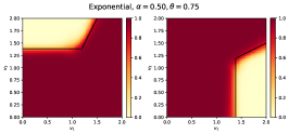
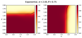
Figure 12: Experiments learned for BIC constraints when the payoffs are drawn from EXP

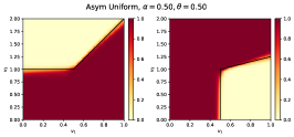
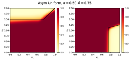
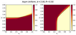
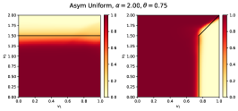
Figure 13: Experiments learned for BIC constraints when the payoffs are drawn from Asym UNF

Distribution	$\alpha$	$\theta$	RegretNet		Opt
			$\mathit{rev}$	$\mathit{rgt}$	$\mathit{rev}$
UNF	0.5	(0.5, 0.5)	0.400	$<0.001$	0.396
		(0.75, 0.25)	0.237		0.237
	2.0	(0.5, 0.5)	1.056		1.042
		(0.75, 0.25)	0.763		0.75
EXP	0.5	(0.5, 0.5)	0.632	$<0.001$	0.632
		(0.75, 0.25)	0.448		0.448
	2.0	(0.5, 0.5)	1.603		1.613
		(0.75, 0.25)	1.390		1.415
Asym UNF	0.5	(0.5, 0.5)	0.614	$<0.001$	0.609
		(0.75, 0.25)	0.366		0.369
	2.0	(0.5, 0.5)	1.599		1.594
		(0.75, 0.25)	1.139		1.135

Figure 14: Test Revenue and Test Regret obtained by RegretNet for the BIC Settings.

G.2 Ex post IC Settings

Figures 15, 16, and 17 show the optimal data market design and the data market learned by RegretNet for the ex post IC settings described above, and Figure 18 gives the test revenue and test regret obtained by RegretNet along with the revenue of the optimal mechanism.

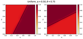
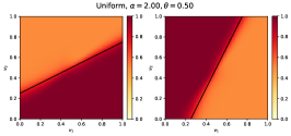
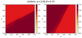
Figure 15: Experiments learned for ex post IC constraints when the payoffs are drawn from UNF

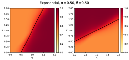
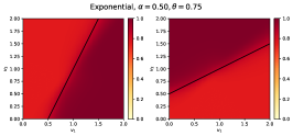
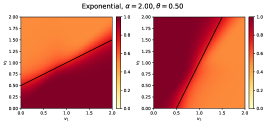
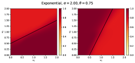
Figure 16: Experiments learned for ex post IC constraints when the payoffs are drawn from EXP

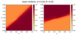
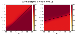
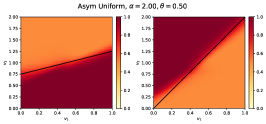
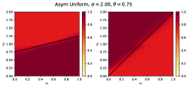
Figure 17: Experiments learned for ex post IC constraints when the payoffs are drawn from Asym UNF

Distribution	$\alpha$	$\theta$	RegretNet		Opt
			$\mathit{rev}$	$\mathit{rgt}$	$\mathit{rev}$
UNF	0.5	(0.5, 0.5)	0.277	$<0.001$	0.27
		(0.75, 0.25)	0.14		0.135
	2.0	(0.5, 0.5)	0.553		0.541
		(0.75, 0.25)	0.278		0.270
EXP	0.5	(0.5, 0.5)	0.405	$<0.001$	0.405
		(0.75, 0.25)	0.204		0.202
	2.0	(0.5, 0.5)	0.801		0.809
		(0.75, 0.25)	0.418		0.405
Asym UNF	0.5	(0.5, 0.5)	0.426	$<0.001$	0.423
		(0.75, 0.25)	0.421		0.21
	2.0	(0.5, 0.5)	0.84		0.841
		(0.75, 0.25)	0.423		0.42

Figure 18: Test Revenue and Test Regret for RegretNet for the ex post IC Settings.

G.3 Additional Results for the Irregular Distributions

We present additional results for both BIC and ex post IC settings for two buyers, binary actions, and interim beliefs $\theta=(0.5,0.5)$, the same for each buyer. We set $\alpha=0.5$, and the payoffs are drawn from the irregular distribution whose pdf $f(v)$ is:

$$f(x)=\begin{cases}2.5,&\text{if }0\leq v<0.3\\ 0.5,&\text{if }0.3\leq v<0.8\end{cases}$$

The optimal solutions for these problems make use of ironed virtual values as the payoff distribution is irregular (see Fig 19).

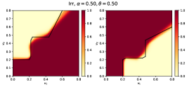
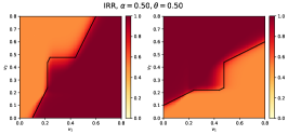
Figure 19: Experiments learned for BIC and ex post IC constraints when the payoffs are drawn from an irregular distribution. For both these settings, we use the ironed virtual value functions to compute the optimal data market design.

Appendix H Proof of Theorem 7

See 7

Proof.

We consider a setting with binary states, binary actions, and where each buyer has the same interim belief, set to $(\theta,1-\theta)$. Without loss of generality, let $\theta\geq(1-\theta)$. Since the interim beliefs are fixed, we will just represent buyer types with $v_{i}$ instead of $\rho_{i}$. Let $x_{i}(v)=\mathop{\mathbb{E}}_{\begin{subarray}{c}a\sim\sigma(\omega;\rho),\\ \omega\sim\theta_{i}\end{subarray}}\left[\mathbf{1}\{a_{i}=\omega\}\right]$. Let $\pi_{i}(v)$ be the matrix representation of the experiment assigned to buyer $i$ i.e. $\pi_{i,\omega}(v)=\sigma_{i}(\omega,v)$

We first show that a mechanism is obedient if and only if the experiment assigned to the buyer satisfies $x_{i}(v)\geq\theta$. If a mechanism is obedient, then $\theta\cdot\pi_{i,1,1}(v)\geq(1-\theta)\pi_{i,2,1}(v)$ and $(1-\theta)\pi_{i,2,2}(v)\geq\theta\cdot\pi_{i,1,2}(v)$. We have $x_{i}(v)=\theta\cdot\pi_{i,1,1}(v)+(1-\theta)\pi_{i,2,2}(v)\geq\theta\cdot\pi_{i,1,1}(v)+\theta\cdot\pi_{i,1,2}(v)=\theta(\pi_{i,1,1}(v)+\pi_{i,1,2}(v))=\theta$.

In the other direction, consider when $x_{i}(v)\geq\theta$. In this case, we show that both $\theta\cdot\pi_{i,1,1}(v)\geq(1-\theta)\pi_{i,2,1}(v)$ and $(1-\theta)\pi_{i,2,2}(v)\geq\theta\cdot\pi_{i,1,2}(v)$ need to hold for obedience. Assume to the contrary, one of these fails to hold when $x_{i}(v)\geq\theta$. We have one of,

• $(1-\theta)\pi_{i,2,2}(v)<\theta\cdot\pi_{i,1,2}(v)$, and we have $x_{i}(v)=\theta\cdot\pi_{i,1,1}(v)+(1-\theta)\pi_{i,2,2}(v)<\theta\cdot\pi_{i,1,1}(v)+\theta\cdot\pi_{i,1,2}(v)=\theta(\pi_{i,1,1}(v)+\pi_{i,1,2}(v))=\theta$.

• $\theta\cdot\pi_{i,1,1}(v)<(1-\theta)\pi_{i,2,1}(v)$, and we have $x_{i}(v)=\theta\cdot\pi_{i,1,1}(v)+(1-\theta)\pi_{i,2,2}(v)<(1-\theta)\pi_{i,2,1}(v)+(1-\theta)\pi_{i,2,2}(v)=(1-\theta)(\pi_{i,2,1}(v)+\pi_{i,2,2}(v))=(1-\theta)\leq\theta$.

In either case, we have a contradiction.

Since our payoff is linear, from Proposition 3.5 in Bergemann et al. [2018], the IC constraints are satisfied only when the truthfulness and obedience constraints are satisfied. Denote $\tilde{x}_{i}(v)=x_{i}(v)-\frac{\alpha}{n-1}\sum_{j\in[n]\setminus i}x_{j}(v)$. Thus, the optimal design problem to solve is:

$$\mathbb{E}_{v\sim\mathcal{V}} \left[\sum_{i\in[n]}t_{i}(v_{i})\right]$$

$$\text{s.t.}\ v_{i}\tilde{x}_{i}(v)-t_{i}(v) \geq v_{i}\tilde{x}_{i}(v^{\prime}_{i};v_{-i})-t_{i}(v^{\prime}_{i};v_{-i})\quad \forall v\in\mathcal{V},v^{\prime}_{i}\in\mathcal{V}_{i},i\in[n]$$

$$v_{i}\tilde{x}_{i}(v)-t_{i}(v) \geq v_{i}(\theta-\alpha)\quad \forall v\in\mathcal{V},i\in[n]$$

$$x_{i}(v) \geq\theta\quad \forall v\in\mathcal{V},i\in[n]$$

The first constraint corresponds to truthfulness for the IC setting, the second is the IR constraint, and the third is the obedience constraint. We have thus reduced the data market design problem to that of Myerson’s revenue maximizing single-item auction problem. Instead of $\tilde{x}_{i}(v)$ denoting the probability of allocating an item, it denotes expected payoff after accounting for the negative externalities. Also, rather than allocative constraints, we have obedience constraints on $x_{i}(v)$ which requires $x_{i}(v)\geq\theta$. Thus, by Myerson’s theory, the total expected revenue is equal to the expected virtual welfare minus some constant $K$ (stemming from IR constraints) for some $\tilde{x}_{i}(v_{i},v_{-i})$ that is non-decreasing in $v_{i}$. Thus, we have:

$$\mathbb{E}_{v\sim\mathcal{V}}\left[\sum_{i\in[n]}[t_{i}(v_{i})]\right] =\mathbb{E}_{v\sim\mathcal{V}}\left[\sum_{i\in[n]}\phi_{i}(v_{i})\tilde{x}_{i}(v)\right]-K$$ (42)

$$=\mathbb{E}_{v\sim\mathcal{V}}\left[\sum_{i\in[n]}\phi_{i}(v_{i})\left(x_{i}(v)-\frac{\alpha}{n-1}\sum_{j\in[n]\setminus i}x_{j}(v)\right)\right]-K$$ (43)

$$=\mathbb{E}_{v\sim\mathcal{V}}\left[\sum_{i\in[n]}\left(\phi_{i}(v_{i})-\frac{\alpha}{n-1}\sum_{j\in[n]\setminus i}\phi_{j}(v_{j})\right)x_{i}(v)\right]-K$$ (44)

In order to maximize the revenue, we need to maximize the virtual welfare. Thus we can set $x_{i}(v)=1$ (a fully informative experiment) when $\phi_{i}(v_{i})-\sum_{j\in[n]\setminus i}\phi_{j}(v_{j})\geq 0$ and we can set $x_{i}(v)=\theta$ (an uninformative experiment that always sends the same signal regardless of the state) otherwise. This is precisely the mechanism described in the theorem.

Note that such an $\tilde{x}_{i}(v_{i},v_{-i})$ is non-decreasing in $v_{i}$ (since $x_{i}(v_{i},v_{-i})$ is non-decreasing in $v_{i}$ and $x_{j}(v_{i},v_{-i})$ for $j\in[n]\setminus i$ is non-increasing in $v_{i}$ for regular distributions $\mathcal{V}_{i}$ and $\mathcal{V}_{j}$). Moreover, $x_{i}(v)\geq\theta$ is also satisfied. ∎

References

- Acemoglu et al. [2022] D. Acemoglu, A. Makhdoumi, A. Malekian, and A. Ozdaglar. Too much data: Prices and inefficiencies in data markets. American Economic Journal: Microeconomics, 14(4):218–256, 2022.
- Acquisti et al. [2016] A. Acquisti, C. Taylor, and L. Wagman. The economics of privacy. Journal of economic Literature, 54(2):442–492, 2016.
- Agarwal et al. [2019] A. Agarwal, M. Dahleh, and T. Sarkar. A marketplace for data: An algorithmic solution. In Proceedings of the 2019 ACM Conference on Economics and Computation, pages 701–726, 2019.
- Agarwal et al. [2020] A. Agarwal, M. Dahleh, T. Horel, and M. Rui. Towards data auctions with externalities. arXiv preprint arXiv:2003.08345, 2020.
- Athey et al. [2017] S. Athey, C. Catalini, and C. Tucker. The digital privacy paradox: Small money, small costs, small talk. Technical report, National Bureau of Economic Research, 2017.
- Babaioff et al. [2012] M. Babaioff, R. Kleinberg, and R. Paes Leme. Optimal mechanisms for selling information. In Proceedings of the 13th ACM Conference on Electronic Commerce, EC ’12, page 92–109, New York, NY, USA, 2012. Association for Computing Machinery. ISBN 9781450314152. doi: 10.1145/2229012.2229024. URL https://doi.org/10.1145/2229012.2229024.
- Bergemann et al. [2018] D. Bergemann, A. Bonatti, and A. Smolin. The design and price of information. American Economic Review, 108(1):1–48, January 2018. doi: 10.1257/aer.20161079. URL https://www.aeaweb.org/articles?id=10.1257/aer.20161079.
- Bergemann et al. [2022a] D. Bergemann, A. Bonatti, and T. Gan. The economics of social data. The RAND Journal of Economics, 53(2):263–296, 2022a. doi: https://doi.org/10.1111/1756-2171.12407. URL https://onlinelibrary.wiley.com/doi/abs/10.1111/1756-2171.12407.
- Bergemann et al. [2022b] D. Bergemann, Y. Cai, G. Velegkas, and M. Zhao. Is selling complete information (approximately) optimal? In Proceedings of the 23rd ACM Conference on Economics and Computation, pages 608–663, 2022b.
- Blackwell [1953] D. Blackwell. Equivalent comparisons of experiments. The annals of mathematical statistics, pages 265–272, 1953.
- Bonatti [2022] A. Bonatti. The platform dimension of digital privacy. Technical report, National Bureau of Economic Research, 2022.
- Bonatti et al. [2022] A. Bonatti, M. Dahleh, T. Horel, and A. Nouripour. Selling information in competitive environments. arXiv preprint arXiv:2202.08780, 2022.
- Cai and Velegkas [2021] Y. Cai and G. Velegkas. How to Sell Information Optimally: An Algorithmic Study. In J. R. Lee, editor, 12th Innovations in Theoretical Computer Science Conference (ITCS 2021), volume 185 of Leibniz International Proceedings in Informatics (LIPIcs), pages 81:1–81:20, Dagstuhl, Germany, 2021. Schloss Dagstuhl–Leibniz-Zentrum für Informatik. ISBN 978-3-95977-177-1. doi: 10.4230/LIPIcs.ITCS.2021.81. URL https://drops.dagstuhl.de/opus/volltexte/2021/13620.
- Cai et al. [2020] Y. Cai, F. Echenique, H. Fu, K. Ligett, A. Wierman, and J. Ziani. Third-party data providers ruin simple mechanisms. Proceedings of the ACM on Measurement and Analysis of Computing Systems, 4(1):1–31, 2020.
- Cai et al. [2021] Y. Cai, A. Oikonomou, G. Velegkas, and M. Zhao. An efficient -bic to BIC transformation and its application to black-box reduction in revenue maximization. In D. Marx, editor, Proceedings of the 2021 ACM-SIAM Symposium on Discrete Algorithms, SODA 2021, Virtual Conference, January 10 - 13, 2021, pages 1337–1356. SIAM, 2021.
- Castiglioni et al. [2022] M. Castiglioni, A. Marchesi, and N. Gatti. Bayesian persuasion meets mechanism design: Going beyond intractability with type reporting. In Proceedings of the 21st International Conference on Autonomous Agents and Multiagent Systems, page 226–234, 2022.
- Chen et al. [2022] J. Chen, M. Li, and H. Xu. Selling data to a machine learner: Pricing via costly signaling. In K. Chaudhuri, S. Jegelka, L. Song, C. Szepesvari, G. Niu, and S. Sabato, editors, Proceedings of the 39th International Conference on Machine Learning, volume 162 of Proceedings of Machine Learning Research, pages 3336–3359. PMLR, 17–23 Jul 2022. URL https://proceedings.mlr.press/v162/chen22m.html.
- Chen et al. [2020] Y. Chen, H. Xu, and S. Zheng. Selling information through consulting. In ACM-SIAM Symposium on Discrete Algorithms (SODA 2020). Presented in ACM/INFORMS Workshop on Market Design 2019, 2020. URL https://arxiv.org/abs/1907.04397.
- Choi et al. [2019] J. P. Choi, D.-S. Jeon, and B.-C. Kim. Privacy and personal data collection with information externalities. Journal of Public Economics, 173:113–124, 2019.