Density-based User Representation through Gaussian Process Regression for Multi-interest Personalized Retrieval

Abstract

Accurate modeling of the diverse and dynamic interests of users remains a significant challenge in the design of personalized recommender systems. Existing user modeling methods, like single-point and multi-point representations, have limitations w.r.t. accuracy, diversity, computational cost, and adaptability. To overcome these deficiencies, we introduce density-based user representations (DURs), a novel model that leverages Gaussian process regression for effective multi-interest recommendation and retrieval. Our approach, GPR4DUR, exploits DURs to capture user interest variability without manual tuning, incorporates uncertainty-awareness, and scales well to large numbers of users. Experiments using real-world offline datasets confirm the adaptability and efficiency of GPR4DUR, while online experiments with simulated users demonstrate its ability to address the exploration-exploitation trade-off by effectively utilizing model uncertainty.

1 Introduction

With the proliferation of online products and services, users have ready access to content, products and services drawn from a vast corpus of candidates. To reduce information overload and to satisfy the diverse needs of users, personalized recommender systems (RSs) play a vital role in reducing information overload and helping users navigate this space. It is widely recognized that users rarely have a single intent or interest when interacting with an RS (Weston et al., 2013; Pal et al., 2020; Cen et al., 2020). To enhance personalization, recent work focuses on discovering a user’s multiple interests and recommending items that cover several of their interests (Cen et al., 2020; Tan et al., 2021; Li et al., 2019). However, this is challenging for two reasons. First, user interests are diverse and dynamic: diversity makes it hard to detect all interests, while their dynamic nature renders determining which user interest is active at any given time quite difficult. Second, it is hard to retrieve items related to niche interests due to the popularity bias (Chen et al., 2020).

User representation is a fundamental design choice in any RS. A key component in capturing multiple interests is a representation that naturally encodes user’s diverse preferences. The most widely used strategy for user modeling is the single-point user representation (SUR), which uses a single point in an item embedding space to represent the user. The user’s affinity for an item is obtained using some distance (e.g., inner product, cosine similarity) with the point representing the item. However, SUR often limits accuracy and diversity of item retrieval (Zhang et al., 2023); hence, most RSs generally use high-dimensional embedding vectors (with high computation cost).

Figure 1: The t-SNE visualization of the prediction score between a picked user to all items in the MovieLens 1M dataset. The triangles ($\blacktriangle$) indicate the latest 20 items interacted by the user. We use Matrix Factorization (MF) to obtain embeddings in this toy example. For the MUR, each user has $K=4$ different embeddings.

To address the limitations of SUR, (Weston et al., 2013) propose MaxMF, which uses a multi-point user representation (MUR), where each user is represented using $K$ points in the embedding space, each reflecting a different “interest”. MaxMF uses a constant, uniform $K$ across all users (e.g., $K=4$), which is somewhat ad hoc and very restrictive. Subsequent research (e.g., PolyDeepWalk (Liu et al., 2019), ComiRec (Cen et al., 2020), SINE (Tan et al., 2021), PIMI (Chen et al., 2021)) uses other heuristic rules and clustering algorithms to determine the number of interests per user (e.g., MIND (Li et al., 2019), PinnerSage (Pal et al., 2020)). However, these all require the manual choice of $K$ or a specific threshold in clustering, limiting the adaptability of MUR methods, since interests generally have high variability across users. Moreover, uncertainty regarding a user’s interests is not well-modeled by these methods, diminishing their ability to perform effective online exploration.

We consider three desiderata of a user representation that are not adequately addressed by SUR and MUR point-based representations: (i) Adaptability, it adapts to different interest patterns; (ii) uncertainty-awareness, it models uncertainty in the assessment of user interests; and (iii) efficiency, it does not require high-dimensional embeddings. These desiderata suggest that user preference representation should be density-based rather than point-based. Specifically, the relevance score for user-item pairs should be higher in regions of embedding space where users have demonstrated a heightened interest in items, and lower in regions where users have shown limited interest in the items present. We propose the density-based user representation (DUR), a novel user modeling method. DUR exploits Gaussian process regression (GPR) (Rasmussen, 2004), a well-studied Bayesian approach to non-parametric regression that uses Gaussian processes (GPs) to extrapolate from training to test data. GPR has been applied across a wide range of domains (Rasmussen and Williams, 2005), though it has been under-explored in user modeling, and multi-interest recommendation and retrieval in particular. We develop a simple and effective means to maintain a unique GP regressor for each user, which serves as our DUR. Given a sequence of user interactions, GPR predicts the probability of a user’s interest in any item using its posterior estimates. We retrieve the top-$N$ items given GPR using a bandit algorithm, e.g., (UCB) (Auer, 2003; Auer et al., 2002), or Thompson Sampling (Russo et al., 2018).

Consider Fig. 1, which shows movies from MovieLens 1M in embedding space (reduced to 2D for visualization). We examine 20 movies from the recent history of a particular user, shown as triangles ($\blacktriangle$) in Fig. 1. As can be seen, the movies come from several different regions in the embedding space. However, when we fit both SUR and MUR models to this data, we see that the models fail to capture the user’s multiple interests and instead assign high scores to movies from only one region in the embedding space (Fig. 1, top row). In contrast, we can see in Fig. 1 bottom left, that GPR can fit the data nicely, assigning high values to regions associated with the user’s recent watches (interests). Fig. 1 bottom right, shows that our approach can also capture uncertainty in user interests, assigning high uncertainty to regions in embedding space where we have fewer samples.

Our approach has a number of desirable properties. First, it adapts to various interest patterns, since the number of interests for any given user is not set manually, but determined by GPR, benefiting from the non-parametric nature of GPs. Second, the Bayesian nature of GPs measures uncertainty with the posterior standard deviation of each item, which supports the incorporation of bandit algorithms in the recommendation and training loop to balance the exploration-exploitation trade-off in online settings. Finally, we demonstrate that our method can effectively retrieve the multiple interests of users, including “niche” interests, while using a lower-dimensional embedding compared to SUR and MUR.

To summarize, our work makes the following contributions:

• We develop GPR4DUR, a density-based user representation method, for personalized multi-interest retrieval. This is the first use of GPR for user modeling in multi-interest setting.

• We propose new evaluation protocols and metrics for multi-interest retrieval that measure the extent to which a model captures a user’s multiple interests.

• We offer comprehensive experiments on real-world offline datasets showing the adaptability and efficiency of GPR4DUR.

• Online experiments with simulated users show the value of GPR4DUR’s uncertainty representation in trading off exploration and exploitation.

2 Related Work

We begin with a discussion of prior work on multi-interest representations and highlight key differences with our approach.

Learning high-quality user representations is central to good RS performance. The single-point user representation (SUR) is the dominant approach, where a user is captured by a single point in some embedding space (Ricci et al., 2011; Rendle et al., 2009), for example, as employed by classical (Koren, 2008; Rendle, 2010; Chen et al., 2018) and neural (He et al., 2017; Liang et al., 2018a) collaborative filtering (CF) methods. While effective and widely used, SUR cannot capture a user’s multiple interests reliably.

To address this limitation, the multi-point user representation (MUR) (Weston et al., 2013) has been proposed, where a user is represented by multiple points in embedding space, each corresponding to a different “primary” interest. Selection of the number of points $K$ is critical in MUR. Existing algorithms largely use heuristic selection methods, e.g., choosing a global constant $K$ for all users (Weston et al., 2013; Liu et al., 2019; Cen et al., 2020; Tan et al., 2021; Chen et al., 2021). Other methods personalize $K$ by letting it be the logarithm of the number of items with which a user has interacted (Li et al., 2019). More recently, Ward clustering of a user’s past items has been proposed, with the user’s $K$ set to be the number of such clusters (Pal et al., 2020). This too requires some manual tuning of the clustering algorithm thresholds.

At inference time MUR is similar to SUR, computing the inner-product of the user embedding(s) and item embedding. Some works compute $K$ inner-products, one per interest, and use the maximum as the recommendation (and the predicted score for that item) (Weston et al., 2013). Others first retrieve the top-$N$ items for each interest ($N\times K$ items), then recommend the top-$N$ items globally (Cen et al., 2020; Pal et al., 2020). None of these methods capture model uncertainty w.r.t. a user’s interests, hence they lack the ability to balance exploration and exploitation in online recommendation in a principled way (Chen, 2021).

Our density-based user representation, and our GPR4DUR algorithm, differs from prior work w.r.t. both problem formulation and methodology. With respect to problem formulation, most prior work on MUR focuses on next-item prediction (Cen et al., 2020; Tan et al., 2021; Li et al., 2019), assuming implicitly a single-stage RS, where the trained model is the main recommendation engine. However, many practical RSs consist of two stages: candidate selection (or retrieval) followed by ranking (Covington et al., 2016a; Borisyuk et al., 2016; Eksombatchai et al., 2018). This naturally raises the question: are the selected candidates diverse enough to cover a user’s interests or intents? This is especially relevant in cases where a user’s dominant interest at the time of recommendation is difficult to discern with high probability; hence, it is important that the ranker have access to a diverse set of candidates that cover the user’s possible range of currently active interests. In this paper, we focus on this retrieval task.

As for methodology, almost all prior work uses point-based representations, either SUR or MUR (Weston et al., 2013; Pal et al., 2020; Cen et al., 2020; Li et al., 2019)—these fail to satisfy all the desiderata outlined in Sec. 1. Instead, we propose the density-based user representation (DUR), a novel method satisfying these criteria, and, to the best of our knowledge, the first to adopt GPR for user modeling in multi-interest recommendation/retrieval.

A related non-parametric approach to recommendations is $k$-nearest-neighbors (kNN). Here, users with similar preferences to the current user are identified (e.g., by similarity in a user embedding space), and the ratings of these users are used to generate recommendations for the current user (see, e.g., (Grcar, 2004)). Our approach differs from kNN in that we do not use user embeddings, but instead fit a GPR model to the item embeddings directly (see Sec. 4.4). This also allows us to account for uncertainty in the user model.

3 Formulation and Preliminaries

In this section, we outline our notation and multi-interest retrieval problem formulation, then, we provide some background on GPR, which lies at the core of our DUR model.

Notation. We consider a scenario where recommended items are attached to category information (e.g., genre for movies). Denote the set of all users, items, and categories by $\mathcal{U}$, $\mathcal{V}$, and $\mathcal{C}$, respectively. For each $u\in\mathcal{U}$, whose interaction history has length $l_{u}$, we partition the sequence of items $\mathcal{V}_{u}$ in $u$’s history into two disjoint lists based on the interaction timestamp (timestamps are monotonic increasing): (i) the history set $\mathcal{V}^{\text{h}}_{u}=[v_{u,1},v_{u,2},...,v_{u,\ell_{u}}]$ serves as the model input; and (ii) the holdout set $\mathcal{V}^{\text{d}}_{u}=[v_{u,{\ell_{u}+1}},v_{u,{\ell_{u}+2}},...,v_{u,l_{u}}]$ is used for evaluation. We define $u$’s interests $\mathcal{C}(\mathcal{V}_{u})$ to be the set of categories associated with all items in $u$’s history. Our notation is summarized in Table 1.

Problem Formulation. We formulate the multi-interest retrieval problem as follows: given $\mathcal{V}^{\text{h}}_{u}$, we aim to retrieve the top-$N$ items $\mathcal{R}_{u}$ (i.e. $|\mathcal{R}_{u}|=N$) w.r.t. some matching metric connecting $\mathcal{R}_{u}$ and $\mathcal{V}^{\text{d}}_{u}$ that measures personalized retrieval performance. We expect $\mathcal{R}_{u}$ to contain relevant items, and given our focus on multi-interest retrieval, $\mathcal{R}_{u}$ should cover all categories in $\mathcal{C}(\mathcal{V}^{\text{d}}_{u})$.

We note that our problem is related to sequential recommendation, where the input is a sequence of interacted items sorted by the timestamp for each user, and the goal is to predict the next item with which the user will interact. By contrast, we focus on retrieving a set of items that cover a user’s diverse interests. We defer the task of generating a precise recommendation list to a downstream ranking model. Unlike, prior work that implicitly represents user interests as item clusters (Pal et al., 2020) or as sub-embeddings (Weston et al., 2013), we define user interests as the set of categories of the items in the user’s history. Such information is widely available in real-world datasets and offers a clear interpretation of user interests, aligning more closely with real-world applications.

Table 1: Description of Notation.

Notation	Description
$\mathcal{U},\mathcal{V},\mathcal{C}$	The set of all users, items, and (item) categories.
$\mathbf{U},\mathbf{V},\mathbf{C}$	Full embedding matrix of users, items, and categories.
$\mathcal{V}_{u}$	The user $u$’s interaction history.
$\mathcal{V}^{\text{h}}_{u},\mathcal{V}^{\text{d}}_{u}$	The history set and holdout set partitioned from $\mathcal{V}_{u}$.
$\mathbf{o}_{u}$	The observed rating scores of $u$ on items in $\mathcal{V}_{u}$.
$t_{u,v}$	The time step when $u$ interacted with $v$.
$l_{u}$	The length of $\mathcal{V}_{u}$.
$\ell_{u}$	The length of user history for model input.
$\mathbf{V}_{u}$	Item embeddings for items in $\mathcal{V}_{u}$.
$\mathcal{R}_{u}$	The list of retrieved items to $u$.
$\mathcal{C}(\cdot)$	The set of categories of all items in the input sequence.

GPR. The core of GPR4DUR is Gaussian process regression (GPR). A Gaussian process (GP) is a flexible probabilistic model used in a variety of applications, such as regression and classification (Rasmussen and Williams, 2005). It is a non-parametric model that defines a prior over functions. GPR employs GPs for regression tasks where the objective is to learn a continuous function given a set of input-output pairs. GPR models a distribution over functions, hence providing not only a point estimate for the target function given any input, but also a measure of uncertainty via predictive variance. This makes GPs a valuable tool for robust decision-making and model-based optimization (Williams and Rasmussen, 1995).

The key components of the GP are the mean function and the covariance (kernel) function, which capture the prior assumptions about the function’s behavior and the relationships between input points, respectively (Rasmussen and Williams, 2005). Let $\mathbf{X}=\{\mathbf{x}_{1},\dots,\mathbf{x}_{n}\}\in\mathbb{R}^{n\times d}$ be a set of input points and $\mathbf{y}=\{y_{1},\dots,y_{n}\}\in\mathbb{R}^{n}$ be the corresponding output values. A GP is defined as:

$$f\sim\mathcal{GP}(\mu,k),$$ (1)

where $\mu(\mathbf{x})$ is the mean function and $k(\mathbf{x},\mathbf{x^{\prime}})$ is the covariance function (kernel). Given a new point $\mathbf{x}_{*}$, the joint distribution of the observed outputs and the output at the new point is given by:

$$\begin{bmatrix}\mathbf{y}\\ f(\mathbf{x}_{*})\end{bmatrix}\sim\mathcal{N}\left(\begin{bmatrix}\bm{\mu}(\mathbf{X})\\ \mu(\mathbf{x}_{*})\end{bmatrix},\begin{bmatrix}\mathbf{K}(\mathbf{X},\mathbf{X})+\sigma^{2}\mathbf{I}&\mathbf{k}(\mathbf{X},\mathbf{x}_{*})\\ \mathbf{k}(\mathbf{x}_{*},\mathbf{X})&k(\mathbf{x}_{*},\mathbf{x}_{*})+\sigma_{*}^{2}\end{bmatrix}\right),$$ (2)

where $\bm{\mu}(\mathbf{X})$ is the vector of mean values for the observed data points, $\mathbf{K}(\mathbf{X},\mathbf{X})$ is the covariance matrix for the observed data points, $\mathbf{k}(\mathbf{X},\mathbf{x}_{*})$ is the vector of covariances between the observed data points and the new input point, and $\sigma^{2}$ and $\sigma_{*}^{2}$ are the noise variances. Without prior observations, $\bm{\mu}$ is generally set as 0.

The conditional distribution of $f(\mathbf{x}_{*})$ given the observed data is:

$$f(\mathbf{x}_{*})|\mathbf{y}\sim\mathcal{N}(\bar{f}_{*},\mathrm{cov}(f_{*})),$$ (3)

with the predictive mean and covariance given by:

$$\bar{f}_{*} =\mu(\mathbf{x}_{*})+\mathbf{k}(\mathbf{x}_{*},\mathbf{X})[\mathbf{K}(\mathbf{X},\mathbf{X})+\sigma^{2}\mathbf{I}]^{-1}(\mathbf{y}-\bm{\mu}),$$ (4)

$$\mathrm{cov}(f_{*}) \!=\!k(\mathbf{x}_{*},\mathbf{x}_{*})\!+\!\sigma_{*}^{2}\!-\!\mathbf{k}(\mathbf{x}_{*},\!\mathbf{X})[\mathbf{K}(\mathbf{X},\mathbf{X})\!+\!\sigma^{2}\mathbf{I}]^{-1}\mathbf{k}(\mathbf{X},\!\mathbf{x}_{*})^{T}.$$ (5)

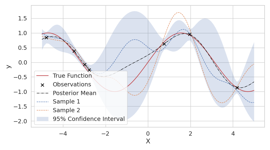
Figure 2: Illustration of Gaussian Process Regression in 1D. The true function is shown in red, observations are marked with black crosses, and the dashed lines represent two samples from the GP posterior. The dash-dot line represents the posterior mean, while the shaded region indicates the 95% confidence interval, showcasing the uncertainty associated with the GP predictions.

Fig. 2 presents a visual illustration of GPR. The true underlying function is depicted in red, which is the function we aim to approximate through GPR. The observations, depicted as black crosses, represent known data points. As expected with GPR, where data points are observed, the uncertainty (represented by the shaded region) is minimal, signifying high confidence in predictions at those locations. On the other hand, in areas without observations, the uncertainty increases, reflecting less confidence in the model’s predictions. The two dashed lines represent samples from the GP posterior. Around observed points, these sampled functions adhere closely to the actual data, representing the power and flexibility of GPR in modeling intricate patterns based on sparse data.

4 Methodology

We now outline our density-based user representation (DUR) using GPR and its application to multi-interest retrieval.

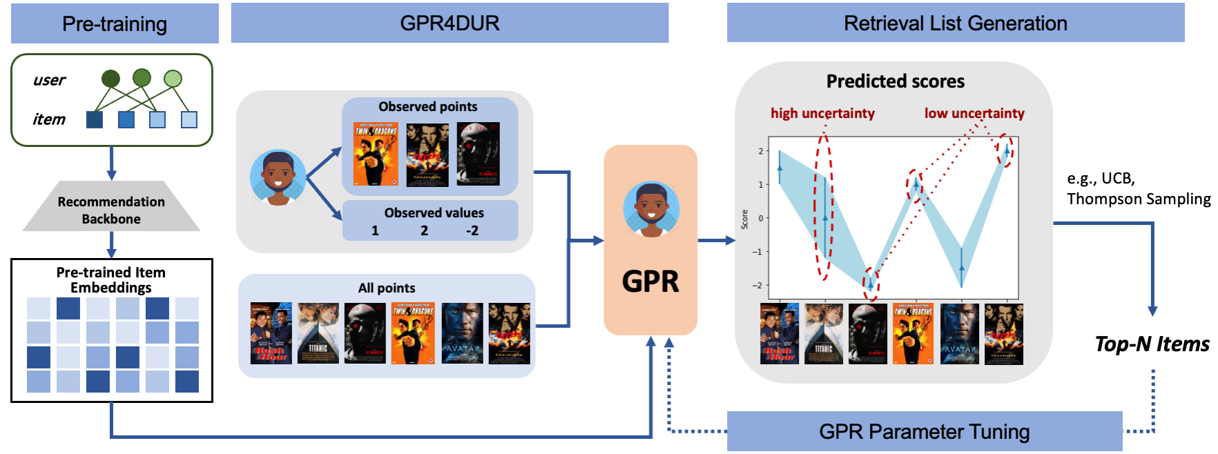
Figure 3: The architecture of GPR4DUR: an example of a movie recommendation for a single user.

4.1 GPR for Density-based User Representation

We now show how to use GPR to construct a novel density-based user representation (DUR) for multi-interest modeling in RSs. Our key insight involves using GPR to learn a DUR, using their interaction history, that naturally embodies their diverse interest patterns. For any user $u$, let $\mathbf{V}_{u}=[\mathbf{v}_{u,1},\mathbf{v}_{u,2},...,\mathbf{v}_{u,l_{u}}]\in\mathbb{R}^{l_{u}\times d}$ be the embeddings of all items in their interaction history. This is derived from their interaction list $\mathcal{V}_{u}$ and an item embedding matrix $\mathbf{V}$ (we describe how to obtain $\mathbf{V}$ in Sec. 4.4). Let $\mathbf{o}_{u}=[o_{u,v}|v\in\mathcal{V}_{u}]\in\mathbb{R}^{l_{u}}$ be the vector of $u$’s observed interactions with items in $\mathcal{V}_{u}$. We employ a GP to model $u$’s interests given the input points $\mathbf{V}_{u}$ and corresponding observations $\mathbf{o}_{u}$ (analogous to Eq. 1),

$$g_{u}\sim\mathcal{GP}(\mu_{u},k_{u}),$$ (6)

where, $g_{u}$, $\mu_{u}$ and $k_{u}$ are $u$’s personalized GP regressor, mean, and kernel function (resp). The joint distribution of observation $\mathbf{o}_{u}$ and the predicted observation of a novel item $v_{*}$ is (as in Eq. 2):

$$\begin{bmatrix}\mathbf{o}_{u}\\ g_{u}(\mathbf{v}_{*})\end{bmatrix}\!\sim\!\mathcal{N}\!\left(\!\begin{bmatrix}\bm{\mu}_{u}(\mathbf{V}_{u})\\ \mu_{u}(\mathbf{v}_{*})\end{bmatrix},\!\begin{bmatrix}\mathbf{K}(\mathbf{V}_{u},\mathbf{V}_{u})\!+\!\sigma^{2}\mathbf{I}&\mathbf{k}(\mathbf{V}_{u},\!\mathbf{v}_{*})\\ \mathbf{k}(\mathbf{v}_{*},\mathbf{V}_{u})&k(\mathbf{v}_{*},\mathbf{v}_{*})\!+\!\sigma_{*}^{2}\end{bmatrix}\!\right)\!.$$ (7)

For simplicity, we assume $\bm{\mu}_{u}=\bm{0}$ and a shared kernel function and variance across all users. In implicit feedback settings, $\mathbf{o}_{u}=\bm{1}$, i.e., $u$ shows “interest” in all interacted items. Thus, the posterior (prediction) $g_{u}(\mathbf{v})$ for any $v\in\mathcal{V}$ is:

$$g_{u}(\mathbf{v})|\mathbf{o}_{u}\sim\mathcal{N}(\bar{g}_{u},\mathrm{cov}(g_{u})),$$

where GP mean $\bar{g}_{u}$ and variance $\text{cov}({g}_{u})$ are:

$$\bar{g}_{u} =\mathbf{k}(\mathbf{v},\mathbf{V}_{u})[\mathbf{K}(\mathbf{V}_{u},\mathbf{V}_{u})+\sigma^{2}\mathbf{I}]^{-1}\mathbf{o}_{u},$$ (8)

$$\mathrm{cov}(g_{u}) =\!k(\mathbf{v},\!\mathbf{v})\!+\!\sigma_{*}^{2}\!-\!\mathbf{k}(\mathbf{v}_{*},\!\mathbf{V}_{u})[\mathbf{K}(\mathbf{V}_{u},\!\mathbf{V}_{u})\!+\!\sigma^{2}\!\mathbf{I}]^{-1}\mathbf{k}(\mathbf{V}_{u},\!\mathbf{v})^{T}\!.$$ (9)

4.2 Retrieval List Generation

After obtaining a DUR $g_{u}$ for $u\in\mathcal{U}$ using GPR, we generate the retrieval list using the posterior $g_{u}(\mathbf{v})$ over all unobserved items. The top-N items with the highest values are selected as our retrieval list. We consider two methods for estimating these values.

The first is Thompson sampling (TS), a probabilistic method that selects items based on posterior sampling (Russo et al., 2018). For each item $v$ in a set, we generate a sample from the posterior $g_{u}(\mathbf{v})$, and rank the items using their sampled values. A key advantage of TS is its ability to balance the trade-off between exploration and exploitation, improving the diversity of the recommendation list. The sampling and selection process is:

$$s_{u,v} \sim g_{u}(\mathbf{v}),\quad\forall v\notin\mathcal{I}_{u},$$ (10)

$$\mathcal{R}_{u} =\text{Top-N}(s_{u,v}),$$ (11)

where $s_{u,v}$ is the value for item $v$ from user $u$’s sampled function, and $\mathcal{R}_{u}$ is the final list of retrieved items for user $u$.

The second method is Upper Confidence Bound (UCB), a deterministic method that selects items based on their estimated rewards and uncertainties (Auer, 2003; Auer et al., 2002). For each item $v$, we compute its upper confidence bound by adding the mean and a confidence interval derived from the variance of the posterior $g_{u}(\mathbf{v})$; items are ranked using these upper bounds. Unlike TS, UCB tends to aggressively promote items with a high degree of posterior uncertainty, giving a different flavor of diversity in the recommendation list. The selection process is:

$$b_{u,v} =\bar{g}_{u}(\mathbf{v})+\beta\cdot\sqrt{\text{var}[{g}_{u}(\mathbf{v})]},\quad\forall v\notin\mathcal{I}_{u},$$ (12)

$$\mathcal{R}_{u} =\text{Top-N}(b_{u,v}),$$ (13)

where $b_{u,v}$ is the upper confidence bound for $v$ w.r.t. $u$’s posterior, and $\beta$ is a hyper-parameter that adjusts the exploration-exploitation trade-off. $\mathcal{R}_{u}$ is the final retrieval list.

4.3 GPR Parameter Tuning

The free parameters in our formulation are the kernel function $\mathbf{K}$ and variance $\sigma^{2}$ in Eq. 7. We treat these as hyperparameters of GPR, optimizing them based on performance evaluation on a separate holdout set. Specifically, to generate $\mathcal{R}_{u}$ for user $u$, we fit the GPR model not to the complete interaction history $\mathcal{V}_{u}$, but to the reduced history $\mathcal{V}^{\text{h}}_{u}$, using the item embeddings and observed ratings. We assess retrieval performance using metrics between $\mathcal{R}_{u}$ and the holdout set $\mathcal{V}^{\text{d}}_{u}$ (metrics are detailed in Sec. 5.3). We tune GPR parameters using these evaluation criteria (we detail the parameters we adjust in Sec. 5.2).

4.4 Item Embedding Pre-training

Following (Pal et al., 2020), we assume that item embeddings are fixed and precomputed: this ensures rapid computation and real-time updates at serving time. For item embedding pre-training, we use extreme multi-class classification, a method widely used in prior work on sequential recommendation (Cen et al., 2020; Kang and McAuley, 2018; Hidasi et al., 2016): given a training sample $(u_{i},v_{j})$, we first compute the likelihood of $u_{i}$ interacting with $v_{j}$, i.e.:

$$p(v_{j}|u_{i})=\frac{\text{exp}(\mathbf{u}_{i}^{\intercal}\mathbf{v}_{j})}{\sum_{v^{\prime}\in\mathcal{V}}\text{exp}(\mathbf{u}_{i}^{\intercal}\mathbf{v}^{\prime})},$$ (14)

where $\mathbf{u}_{i}$ and $\mathbf{v}_{j}$ are embeddings of $u_{i}$ and $v_{j}$. Our objective is to maximize the log-likelihood of the probability of a user interacting with their items.

However, we want not just to capture the user-item interaction matrix, but also to ensure that item embeddings align with the categories to which they belong, since categories explicitly indicate a user’s interests. We capture item-category information by computing the likelihood that an item belongs to a category (analogous to Eq. 14):

$$p(c_{k}|v_{j})=\frac{\text{exp}(\mathbf{v}_{j}^{\intercal}\mathbf{c}_{k})}{\sum_{c^{\prime}\in\mathcal{C}}\text{exp}(\mathbf{v}_{j}^{\intercal}\mathbf{c}^{\prime})}.$$ (15)

The overall objective for pre-training is a combination of the two negative log-likelihoods using a scaling factor $\gamma$:

$$\mathcal{L}=\sum_{u_{i}}\sum_{v_{j}\in\mathcal{V}_{u_{i}}}-\log p(v_{j}|u_{i})+\gamma\cdot\sum_{v_{j}}\sum_{c_{k}\in\mathcal{C}_{v_{j}}}-\log p(c_{k}|v_{j}),$$ (16)

where $\mathcal{V}_{u_{i}}$ is the set of items that $u_{i}$ interacted with and $\mathcal{C}_{v_{j}}$ is the set of categories that $v_{j}$ belongs to. The full item embedding matrix $\mathbf{V}$ is jointly learned and fixed after the pre-training phase. Notice that we do not use the user and category embeddings after pre-training, and other schemes for computing item embeddings are possible. The full architecture for GPR4DUR is shown in Fig. 3.

5 Offline Experiments

We first evaluate our GPR4DUR on three real-world datasets, and compare our DUR technique with other state-of-the-art methods for multi-interest retrieval.

Table 2: Result comparison across all methods on different metrics and datasets. For the same metric on each dataset, the best is bold, while the second best is underlined. We use different poker symbols to indicate the four different categories of the methods as demonstrated in Sec. 5. Our proposed GPR4DUR has a statistical significance for $p\leq 0.01$ compared to the best baseline method (labelled with *) based on the paired t-test.

Methods	Interest Coverage (IC@$k$)			Interest Relevance (IR@$k$)			Exp. Deviation (ED@$k$)			Tail Exp. Improv. (TEI@$k$)
	The higher the better $\Uparrow$			The higher the better $\Uparrow$			The lower the better $\Downarrow$			The higher the better $\Uparrow$
	$k=20$	$k=50$	$k=100$	$k=20$	$k=50$	$k=100$	$k=20$	$k=50$	$k=100$	$k=20$	$k=50$	$k=100$
MovieLens 1M
$\clubsuit$ Random	0.7873	0.9290	0.9786	0.4011	0.5693	0.6765	0.3244	0.3029	0.2939	-0.1620	-0.1628	-0.1624
$\clubsuit$ MostPop	0.7959	0.9609∗	0.9838	0.4647	0.6482	0.7611	0.3279	0.3165	0.2981	-0.0816∗	-0.0922	-0.1215
$\vardiamondsuit$ YoutubeDNN	0.7910	0.9464	0.9866	0.7230∗	0.8516	0.8949∗	0.3408	0.3175	0.3059	-0.1050	-0.1318	-0.1400
$\vardiamondsuit$ GRU4REC	0.7336	0.8794	0.9463	0.5759	0.7252	0.8196	0.2998∗	0.2829∗	0.2725	-0.0824	-0.0907∗	-0.1003∗
$\spadesuit$ MIND	0.8067	0.9467	0.9881	0.6826	0.8053	0.8713	0.3420	0.3152	0.3054	-0.0973	-0.1241	-0.1362
$\spadesuit$ ComiRec	0.8356∗	0.9342	0.9873	0.7078	0.7801	0.8152	0.3348	0.3161	0.3065	-0.1022	-0.1292	-0.1326
$\varheartsuit$ GPR4DUR	0.9301	0.9755	0.9877	0.7309	0.8436	0.9021	0.2913	0.2806	0.2763	-0.0585	-0.0713	-0.0809
Amazon CD
$\clubsuit$ Random	0.6902	0.8876∗	0.9611	0.2511	0.4275	0.5584	0.5128	0.4834	0.4720	-0.0405	-0.0407	-0.0408
$\clubsuit$ MostPop	0.7037∗	0.7658	0.7879	0.3241	0.4264	0.4900	0.5630	0.5009	0.4851	-0.0449	-0.0449	-0.0449
$\vardiamondsuit$ YoutubeDNN	0.6720	0.8095	0.8778	0.4323	0.5501∗	0.6228∗	0.4699∗	0.4389	0.4228	-0.0398	-0.0410	-0.0401
$\vardiamondsuit$ GRU4REC	0.6759	0.8096	0.8837	0.4145	0.5242	0.6023	0.4851	0.4516	0.4375	-0.0403	-0.0401	-0.0401
$\spadesuit$ MIND	0.6498	0.7874	0.8614	0.3896	0.5027	0.5752	0.5091	0.4774	0.4609	-0.0405	-0.0410	-0.0414
$\spadesuit$ ComiRec	0.6558	0.7845	0.8613	0.3986	0.5099	0.5949	0.4918	0.4529	0.4324	-0.0400	-0.0399	-0.0398∗
$\varheartsuit$ GPR4DUR	0.7388	0.8945	0.9556	0.4290	0.5604	0.6426	0.4577	0.4226	0.4120	-0.0408	-0.0392	-0.0389
MovieLens 20M
$\clubsuit$ Random	0.8347	0.9609	0.9915	0.2719	0.4224	0.5341	0.2523	0.2291	0.2212	-0.1853	-0.1838	-0.1834
$\clubsuit$ MostPop	0.9138∗	0.9729∗	0.9857	0.4978	0.6549	0.7265	0.2612	0.2227	0.2174	-0.0217	-0.0128∗	-0.0284∗
$\vardiamondsuit$ YoutubeDNN	0.8794	0.9378	0.9743	0.7217∗	0.8456∗	0.8726∗	0.2496	0.2294	0.2181	-0.0170∗	-0.0306	-0.0513
$\vardiamondsuit$ GRU4REC	0.8317	0.9385	0.9761	0.6458	0.7841	0.8632	0.2281	0.2259	0.1947	-0.0702	-0.0759	-0.0838
$\spadesuit$ MIND	0.8686	0.9512	0.9814	0.6529	0.7859	0.8634	0.2451	0.2233	0.2117	-0.0485	-0.0578	-0.0734
$\spadesuit$ ComiRec	0.8436	0.9456	0.9806	0.6347	0.7762	0.8585	0.2267	0.2026	0.1921	-0.0692	-0.0743	-0.0820
$\varheartsuit$ GPR4DUR	0.9293	0.9738	0.9734	0.8253	0.8620	0.8907	0.2517	0.2216	0.2012	-0.0107	-0.0069	-0.0163

5.1 Datasets

We use three widely studied benchmark datasets: MovieLens 1M (Harper and Konstan, 2015), MovieLens 20M (Harper and Konstan, 2015), and Amazon CD (He and McAuley, 2016). We adopt the setting as previous works (Li et al., 2020; Wang et al., 2019), filtering out items that appear fewer than 10 times in the dataset, and users who interact with fewer than 25 items. This ensures users have sufficient interaction history to indicate multiple interests. For the MovieLens datasets, we use the 18 movie genres as categories, where each movie can belong to multiple categories. For Amazon CD, we use the single principle category of each item. Each category reflects a unique user interest. Dataset statistics are shown in Table 3.

Table 3: The statistics of datasets.

	MovieLens 1M	Amazon CD	MovieLens 20M
# User / Item	5,611 / 2,934	6,223 / 32,830	123,002 / 12,532
# Interac.	983,753	368,900	19,584,266
# Avg. Interac.	175.33	59.28	159.22
# Category (Interest)	18	28	18

5.2 Experiment Setup

Most prior work on recommendation and retrieval evaluates model performance on generalization to new items per user. Instead, similar to recent work (Liang et al., 2018b; Cen et al., 2020), we assess model performance on a more challenging measure: its ability to generalize to new users. We split users into disjoint subsets: training users ($\mathcal{U}^{\text{train}}$), validation users ($\mathcal{U}^{\text{val}}$), and test users ($\mathcal{U}^{\text{test}}$) at a ratio of 8:1:1. We treat the last 20% of a user’s full interaction sequence as a holdout set for evaluation, and the first 80% as a history set used to fit the model. We set the history length thresholds for the three datasets to 175, 60, and 160, respectively. These values correspond to the average number of user interactions in each dataset.

For the item embedding pre-training phase, we train the recommendation backbones using the history set of all training users and tune the parameters based on the performance on the holdout set for validation users. The maximum training iteration is set to 100,000. An early stopping strategy is used if performance on the validation set does not improve for 50 successive iterations. For GPR parameter tuning, we fit the history set of all training users and validation users to the GP regressor to learn their user representations, then tune the parameters (i.e., kernel $k$ and variance $\sigma$) using the holdout set. For a fair comparison across all methods, we report measurements on the holdout set for all test users.

5.3 Metrics

Metrics used in prior work on sequential recommendation are not well-suited to measure performance in our multi-interest retrieval task. This is true for several reasons: (i) Conventional metrics, such as precision and recall, often employed in multi-interest research, do not adequately quantify whether an item list fully reflects a user’s full range of (multiple) interests. A model may primarily recommend items from a narrow range of highly popular categories and still score high on these metrics while potentially overlooking less popular or niche interests. (ii) Metrics like precision and recall are overly stringent, only recognizing items in the recommendation list that appear in the holdout set. We argue that credit should also be given if a similar, though not identical, item is recommended (e.g., Iron Man 1 and Iron Man 2 should be considered highly similar). This requires a softer version of these metrics. (iii) Retrieval systems with multi-interest capabilities should aim to provide exposure for items from niche interests in order to cover potential interests of the user in question. However, traditional metrics often overlook the item perspective, increasing the risk of underserving users with specific niche interests. Consequently, we propose the use of the following four metrics, encompassing all the aforementioned facets, for evaluating approaches to multi-interest recommendation:

Interest-wise Coverage (IC)

This metric is similar to subtopic-recall (Zhai et al., 2003), which directly measures whether the model can comprehensively retrieve all the user interests indicated in the holdout set. The higher the value of this metric the better:

$$\text{IC}@k=\frac{1}{|\mathcal{U}^{\text{test}}|}\sum_{u\in\mathcal{U}^{\text{test}}}\frac{|\mathcal{C}(\mathcal{V}^{\text{d}}_{u})\cap\mathcal{C}(\mathcal{R}^{1:k}_{u})|}{|\mathcal{C}(\mathcal{V}^{\text{d}}_{u})|}.$$ (17)

Interest-wise Relevance (IR)

In addition to capturing all user interests based on item categories, it is important to ensure that the retrieved items are relevant to the user. To address this, we propose a soft version of the conventional recall metric by calculating the maximum cosine similarity between items in the retrieval list and the holdout set within the same category. The motivation is that the success of a retrieval or recommendation list often depends on how satisfying the most relevant item is:

$$\text{IR}@k =\frac{1}{|\mathcal{U}^{\text{test}}|}\sum_{u\in\mathcal{U}^{\text{test}}}\frac{\sum\limits_{c\in\mathcal{C}(\mathcal{V}^{\text{d}}_{u})}\max\limits_{v_{i}\in\mathcal{V}^{\text{d}}_{u},v_{j}\in\mathcal{R}^{1:k}_{u}}S(v_{i},v_{j})}{|\mathcal{C}(\mathcal{V}^{\text{d}}_{u})|},$$ (18)

s.t., $$\mathcal{C}(v_{i})=\mathcal{C}(v_{j})=c,$$

where $S(v_{i},v_{j})$ is the cosine similarity between item $v_{i}$ and $v_{j}$. To obtain ground-truth similarities between items, and to mitigate the influence of the chosen pre-trained model, we pretrain the item embeddings using YoutubeDNN (Covington et al., 2016b) with a higher dimension size ($d=256$) to compute a uniform $\mathbf{S}_{i,j}$ for any backbone. A higher value of this metric is better.

Exposure Deviation (ED)

In addition to measuring performance from the user perspective, we also measure from the point-of-view of items to test whether exposure of different categories in the retrieval list is close to that in the holdout set. We treat each occurrence of an item category as one unit of exposure, and compute the normalized exposure vectors $\epsilon_{u}^{*},\epsilon_{u}^{1:k}\in\mathbb{R}^{|\mathcal{C}|}$ for $u$’s holdout set and retrieval list, respectively. Lower values of this metric are better:

$$\text{ED}@k =\frac{1}{|\mathcal{U}^{\text{test}}|}\sum\limits_{u\in\mathcal{U}^{\text{test}}}||\epsilon^{*}_{u}-\epsilon_{u}^{1:k}||_{2}^{2},$$ (19)

s.t., $$\epsilon^{*}_{u,c}=\frac{\sum_{v\in\mathcal{V}^{\text{d}}_{u}}\mathbbm{1}_{{c\in\mathcal{C}(v)}}}{\sum_{v\in\mathcal{V}^{\text{d}}_{u}}|\mathcal{C}(v)|},\epsilon^{1:k}_{u,c}=\frac{\sum_{v\in\mathcal{R}^{1:k}_{u}}\mathbbm{1}_{{c\in\mathcal{C}(v)}}}{\sum_{v\in\mathcal{R}^{1:k}_{u}}|\mathcal{C}(v)|}.$$ (20)

Tail Exposure Improvement (TEI)

With respect to category exposure, it is crucial to ensure that niche interests are not under-exposed. To evaluate this, we select a subset of the least popular categories and measure their exposure improvement in the retrieval list versus that in the holdout set. A higher value of this metric indicates better performance, and a positive value indicates improvement:

$$\text{TEI}@k =\frac{1}{|\mathcal{U}^{\text{test}}|}\sum\limits_{u\in\mathcal{U}^{\text{test}}}\sum\limits_{c\in\mathcal{C}^{\text{tail}}}(\epsilon_{u,c}^{1:k}-\epsilon^{*}_{u,c})\mathbbm{1}_{\epsilon^{*}_{u,c}>0}.$$ (21)

Here, $\mathcal{C}^{\text{tail}}$ refers to the set of niche categories (i.e., the last 50% long-tail categories), denoting those niche interests. $\mathbbm{1}_{\epsilon^{*}_{u,c}>0}$ indicates that we only compute the improvement for categories that appear in the user’s holdout set, reflecting their true interests.

5.4 Methods Studied

Figure 4: Methods comparison across different user groups on MovieLens 20M. Best view in color.

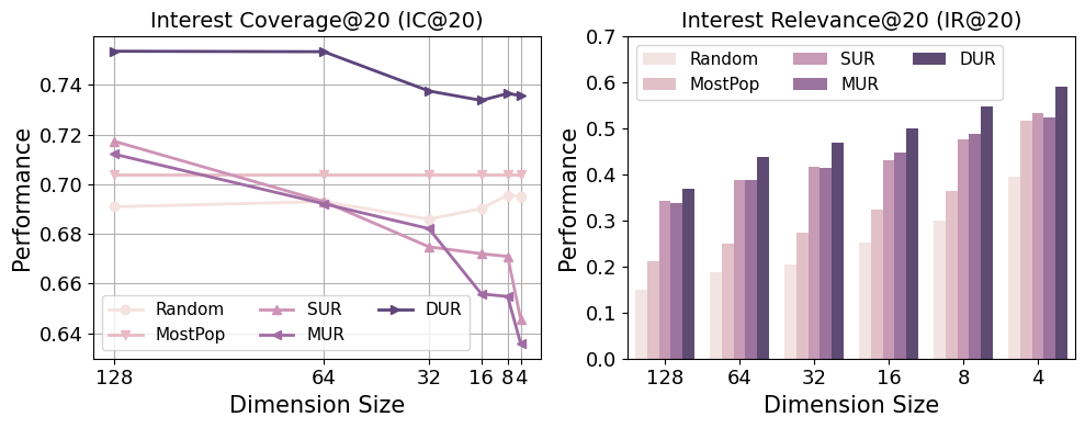
Figure 5: Robustness comparison across different dimension sizes on Amazon CD. Best view in color.

We study the following seven methods from four categories.

(i) Heuristic-based Methods $\clubsuit$ :

• Random always randomly recommends items to users.

• MostPop always recommends the most popular items.

(ii) SUR-based Methods $\vardiamondsuit$ :

• YoutubeDNN (Covington et al., 2016b) is one of the most successful deep learning models for industrial recommendation platforms.

• GRU4REC (Hidasi et al., 2016) is the first work that introduces recurrent neural networks for the recommendation.

(iii) MUR-based Methods $\spadesuit$ :

• MIND (Li et al., 2019) designs a multi-interest extractor layer based on the capsule routing mechanism, which is applicable for clustering past behaviors and extracting diverse interests.

• ComiRec (Cen et al., 2020) is one of the SOTA methods that captures multiple interests from user behavior sequences with a controller for balancing diversity.

(iv) DUR-based Method (Ours) $\varheartsuit$ :

• GPR4DUR uses GPR as a density-based user representation tool for capturing users’ diverse interests with uncertainty.

5.4.1 Overall Performance Comparison

The overall performance comparison addresses two central research questions: whether our proposed method, GPR4DUR, can demonstrate superior performance in the retrieval of multi-interests for users (RQ1), and whether it can ensure appropriate item-sided exposure for retrieving both popular and niche interests (RQ2).

For RQ1, our focus lies in assessing the effectiveness of the retrieval process. As illustrated in Table 2, GPR4DUR consistently outperforms the baseline methods across all datasets in most cases on Interest Coverage (IC@$k$) and Interest Relevance (IR@$k$) across all values of $k$, denoting the strong coverage and relevance of the retrieval respectively. For instance, on the MovieLens 20M dataset, GPR4DUR achieves the best on 5 out of 6 interest metrics. This illustrates that GPR4DUR can not only cover a wide range of user interests but also maintain high relevance.

For RQ2, our objective is to ascertain that item exposure is appropriately balanced. We measure this through the Exposure Deviation (ED@$k$) and Tail Exposure Improvement (TEI@$k$) metrics. Lower values of ED@$k$ suggest more satisfying category exposure compared to the holdout set, while higher values of TEI@$k$ are indicative of enhanced exposure in the long tail of item categories. In these regards, GPR4DUR demonstrates considerable effectiveness, consistently performing well across all datasets in most instances. This validates its utility in guaranteeing an optimal level of item category exposure. A notable example is that GPR4DUR shows the best results in 8 out of 9 TEI@$k$ metrics, indicating its superior capability in providing exposure to niche categories / interests. However, we emphasize that all TEI@$k$ values are negative, which suggests that none of the evaluated methods could improve exposure for niche categories relative to the exposure found in users’ holdout sets. This aligns with the known issue of popularity bias inherent in most recommendation methods, indicating that more work is required on diversification strategies to mitigate such effects.

5.4.2 Performance across User Groups (RQ3)

We further conduct a more fine-grained analysis on the performance across five different user groups with equal size (i.e., $g1$ to $g5$) based on the ascending order of their degrees, where a degree refers to the number of interactions or the number of interests. Due to the page limitation, we only show the results comparison on IR@20 and TEI@20 across different models on MovieLens 20M, and we only display the best model for both SUR and MUR strategies. The DUR denotes our proposed method GPR4DUR. As shown in Fig. 4, our method consistently surpasses all the other methods in terms of both relevance and exposure metrics. The improvement becomes more pronounced as the user degree rises. Interestingly, while no model can enhance the overall exposure of niche interests as displayed in Table 2, our method can considerably increase the exposure of those niche interests for users with high degrees (i.e., the TEI@20 metric is positive on $g4$ and $g5$ using our DUR-based method). These observations strongly affirm the effectiveness of our method in capturing user’s multiple interests, especially for those high-degree users, and its potential to maintain fair exposure on the item side.

5.4.3 Robustness to Dimension Size (RQ4)

We underscored the importance of efficiency for a good user representation in Sec. 1. To shed light on this aspect, we examine the IC@20 and IR@20 metrics generated by various methods on Amazon CD. As shown in Fig. 5, on the interest coverage, our method successfully maintains a high performance even when operating in low dimensions (i.e., $d=8$ and $d=4$). In contrast, SUR and MUR methods degrade in performance as the dimension decreases. As for the interest relevance, our method still consistently outperforms other methods across all dimensions. A noteworthy point is that when lower dimensions are employed, a higher interest relevance tends to be more readily achievable due to the cosine similarity in Eq. 18. This is why the value of IR@20 increases as the dimension size decreases.

6 Online Simulation

To demonstrate the efficacy of GPR4DUR in capturing uncertainty in user interest exploration, we conduct an online simulation in a purely synthetic setting, using a specific model of stochastic user behavior to reflect responses to recommendations.

Data Preparation. We start by defining $|\mathcal{C}|=10$ total interest clusters, each represented by a $d$-dim ($d=32$) multivariate Gaussian distribution. We randomly select a (user-specific) subset of these interests as the ground-truth interests for each user. We set $|\mathcal{U}|=1000$ and $|\mathcal{V}|=3000$, with $300$ items for each interest cluster. Each item belongs to a single interest cluster and the item embedding is sampled from the corresponding interest distribution. Each user is modeled by a multi-modal Gaussian, a weighted sum of the corresponding ground-truth interest distributions. To simulate a sequence of item interactions $\mathcal{V}_{u}$ (i.e., user history), we follow (Mehta et al., 2023) to first run a Markov Chain using a predefined user interest transition matrix to obtain the user’s interacted interest sequence for $S=10$ steps. In this experiment, we do not consider the cold-start problem, so we recommend one item from each generated interest cluster to form the user history (i.e., $|\mathcal{V}_{u}|=S$). The user observation $\mathbf{o}_{u}$ on items in $\mathcal{V}_{u}$ is set to 1 if the item belongs to a ground-truth interest cluster, otherwise -1.

GPR Fit and Prediction. After obtaining the item embeddings $\mathbf{V}$, user history $\mathcal{V}_{u}$, and user observation $\mathbf{o}_{u}$, we use GPR to obtain a density-based user representation for each user, using the methods described in Sec. 4.

User History and Observation Update. Using a predetermined user browsing model, clicked and skipped items are identified and appended to the user history, updating our record of user interactions. The corresponding user observation is updated simultaneously (1 for clicked items, -1 for skipped). This update process continues until the maximum iteration count $T=10$ is reached. In this online setting, we employ the dependent click Model (DCM) of user browsing behavior, widely used in web search and recommendation (Cao et al., 2020; Chuklin et al., 2015). In the DCM, users begin with the top-ranked item, progressing down the list, engaging with items of interest and deciding to continue or terminate after each viewed item.

Experiment Results. We conduct evaluation by measuring the proposed metrics at each iteration between different policies (for lack of space we only report results for interest coverage). We test whether policies that use uncertainty models outperform those that do not. Specifically, we compute a “cumulative” version of interest coverage by reporting the interest coverage averaged across all users on all previously recommended items prior to the current iteration. We assume each policy recommends the top-10 items to each user at each iteration. Table 4 shows that methods using uncertainty (the bottom three rows) fairly reliably outperform those that do not (the top two rows, with Greedy being UCB with $\beta=0$). The observation confirms the benefit of using GPR4DUR to explicitly model uncertainty in user interests and to drive exploration.

Table 4: Comparison between different policies in online setting. The reported values are the interest coverage averaged across all users on all cumulative recommended items up to each iteration. The highest value of each column is in bold.

Policy	$t$=1	$t$=2	$t$=3	$t$=4	$t$=5	$t$=6	$t$=7	$t$=8	$t$=9	$t$=10
Random	0.29	0.49	0.64	0.74	0.82	0.87	0.91	0.91	0.92	0.93
Greedy	0.71	0.88	0.90	0.90	0.91	0.91	0.91	0.92	0.92	0.92
UCB ($\beta$=1)	0.71	0.89	0.91	0.91	0.92	0.92	0.92	0.93	0.94	0.95
UCB ($\beta$=5)	0.72	0.88	0.90	0.90	0.91	0.91	0.92	0.92	0.93	0.94
Thompson	0.29	0.50	0.65	0.75	0.82	0.89	0.91	0.92	0.95	0.98

7 Conclusion and Discussion

Conclusion. In this paper, we introduce a density-based user representation model, GPR4DUR, marking the first application of Gaussian Process Regression for user modeling in multi-interest retrieval. This innovative approach inherently captures dynamic user interest, provides uncertainty-awareness, and proves to be more efficient than traditional point-based methods. We also establish a new evaluation protocol and metrics specifically tailored for multi-interest retrieval tasks, filling a gap in the current evaluation landscape. Offline experiments validate the adaptability and efficiency of GPR4DUR, demonstrating its superiority over existing models. Online simulations further highlight GPR4DUR’s aptitude in user interest exploration by effectively leveraging model uncertainty.

Discussion. While it is true that Gaussian Process Regression has a computational complexity of $O(N^{3})$ with respect to the number of observations $N$, this complexity is actually relative to a user’s interaction history, rather than the entire set of items available in the domain. In practice, given the typically sparse user interaction data relative to the total item count, this cubic complexity is often quite manageable. Moreover, an effective way to tackle the computational demand of GPR is to impose a limit on the length of a user’s interaction history, and only consider the most recent interactions or a representative set of interactions if the length exceeds the threshold. This strategy not only helps to control the computational complexity, but can also ensure that the model is primarily influenced by the most recent and relevant user interactions, thus making GPR more applicable and efficient in real-world recommendation systems.

For future research, the incorporation of collaborative Gaussian Processes presents a tantalizing prospect. Our current model primarily focuses on personalization, using the other users solely for the tuning of GPR hyperparameters. However, we postulate that harnessing the power of collaborative learning (e.g., (Houlsby et al., 2012)) could further enhance the performance and effectiveness of our approach.

References

- (1)
- Auer (2003) Peter Auer. 2003. Using Confidence Bounds for Exploitation-Exploration Trade-Offs. J. Mach. Learn. Res. 3 (mar 2003), 397–422.
- Auer et al. (2002) Peter Auer, Nicolò Cesa-Bianchi, and Paul Fischer. 2002. Finite-Time Analysis of the Multiarmed Bandit Problem. Mach. Learn. 47, 2–3 (may 2002), 235–256.
- Borisyuk et al. (2016) Fedor Borisyuk, Krishnaram Kenthapadi, David Stein, and Bo Zhao. 2016. CaSMoS: A framework for learning candidate selection models over structured queries and documents. In Proceedings of the 22nd ACM SIGKDD International Conference on Knowledge Discovery and Data Mining. 441–450.
- Cao et al. (2020) Junyu Cao, Wei Sun, Zuo jun Max Shen, and Markus Ettl. 2020. Fatigue-Aware Bandits for Dependent Click Models. ArXiv abs/2008.09733 (2020).
- Cen et al. (2020) Yukuo Cen, Jianwei Zhang, Xu Zou, Chang Zhou, Hongxia Yang, and Jie Tang. 2020. Controllable Multi-Interest Framework for Recommendation. In KDD ’20: The 26th ACM SIGKDD Conference on Knowledge Discovery and Data Mining, Virtual Event, CA, USA, August 23-27, 2020. ACM, 2942–2951.
- Chen et al. (2021) Gaode Chen, Xinghua Zhang, Yanyan Zhao, Cong Xue, and Ji Xiang. 2021. Exploring Periodicity and Interactivity in Multi-Interest Framework for Sequential Recommendation. In Proceedings of the Thirtieth International Joint Conference on Artificial Intelligence, IJCAI 2021, Virtual Event / Montreal, Canada, 19-27 August 2021. ijcai.org, 1426–1433.
- Chen et al. (2020) Jiawei Chen, Hande Dong, Xiang Wang, Fuli Feng, Meng Wang, and Xiangnan He. 2020. Bias and Debias in Recommender System: A Survey and Future Directions. CoRR abs/2010.03240 (2020).
- Chen (2021) Minmin Chen. 2021. Exploration in Recommender Systems. In RecSys ’21: Fifteenth ACM Conference on Recommender Systems, Amsterdam, The Netherlands, 27 September 2021 - 1 October 2021. ACM, 551–553.
- Chen et al. (2018) Rui Chen, Qingyi Hua, Yan-shuo Chang, Bo Wang, Lei Zhang, and Xiangjie Kong. 2018. A Survey of Collaborative Filtering-Based Recommender Systems: From Traditional Methods to Hybrid Methods Based on Social Networks. IEEE Access 6 (2018), 64301–64320.
- Chuklin et al. (2015) Aleksandr Chuklin, Ilya Markov, and Maarten de Rijke. 2015. Click Models for Web Search. Morgan & Claypool. https://doi.org/10.2200/S00654ED1V01Y201507ICR043
- Covington et al. (2016a) Paul Covington, Jay Adams, and Emre Sargin. 2016a. Deep neural networks for youtube recommendations. In Proceedings of the 10th ACM conference on recommender systems. 191–198.
- Covington et al. (2016b) Paul Covington, Jay Adams, and Emre Sargin. 2016b. Deep Neural Networks for YouTube Recommendations. In Proceedings of the 10th ACM Conference on Recommender Systems, Boston, MA, USA, September 15-19, 2016. ACM, 191–198.
- Eksombatchai et al. (2018) Chantat Eksombatchai, Pranav Jindal, Jerry Zitao Liu, Yuchen Liu, Rahul Sharma, Charles Sugnet, Mark Ulrich, and Jure Leskovec. 2018. Pixie: A system for recommending 3+ billion items to 200+ million users in real-time. In Proceedings of the 2018 world wide web conference. 1775–1784.
- Grcar (2004) Miha Grcar. 2004. User profiling: Collaborative filtering. In Proceedings of SIKDD 2004 at Multiconference IS. 75–78.
- Harper and Konstan (2015) F. Maxwell Harper and Joseph A. Konstan. 2015. The MovieLens Datasets: History and Context. 5, 4 (2015).
- He and McAuley (2016) Ruining He and Julian J. McAuley. 2016. Ups and Downs: Modeling the Visual Evolution of Fashion Trends with One-Class Collaborative Filtering. In WWW. ACM, 507–517.
- He et al. (2017) Xiangnan He, Lizi Liao, Hanwang Zhang, Liqiang Nie, Xia Hu, and Tat-Seng Chua. 2017. Neural Collaborative Filtering. In Proceedings of the 26th International Conference on World Wide Web, WWW 2017, Perth, Australia, April 3-7, 2017, Rick Barrett, Rick Cummings, Eugene Agichtein, and Evgeniy Gabrilovich (Eds.). ACM, 173–182.
- Hidasi et al. (2016) Balázs Hidasi, Alexandros Karatzoglou, Linas Baltrunas, and Domonkos Tikk. 2016. Session-based Recommendations with Recurrent Neural Networks. In 4th International Conference on Learning Representations, ICLR 2016, San Juan, Puerto Rico, May 2-4, 2016, Conference Track Proceedings.
- Houlsby et al. (2012) Neil Houlsby, Ferenc Huszar, Zoubin Ghahramani, and Jose Hernández-lobato. 2012. Collaborative gaussian processes for preference learning. Advances in neural information processing systems 25 (2012).
- Kang and McAuley (2018) Wang-Cheng Kang and Julian J. McAuley. 2018. Self-Attentive Sequential Recommendation. In IEEE International Conference on Data Mining, ICDM 2018, Singapore, November 17-20, 2018. IEEE Computer Society, 197–206.
- Koren (2008) Yehuda Koren. 2008. Factorization meets the neighborhood: a multifaceted collaborative filtering model. In Proceedings of the 14th ACM SIGKDD International Conference on Knowledge Discovery and Data Mining, Las Vegas, Nevada, USA, August 24-27, 2008, Ying Li, Bing Liu, and Sunita Sarawagi (Eds.). ACM, 426–434.
- Li et al. (2019) Chao Li, Zhiyuan Liu, Mengmeng Wu, Yuchi Xu, Huan Zhao, Pipei Huang, Guoliang Kang, Qiwei Chen, Wei Li, and Dik Lun Lee. 2019. Multi-Interest Network with Dynamic Routing for Recommendation at Tmall. In Proceedings of the 28th ACM International Conference on Information and Knowledge Management, CIKM 2019, Beijing, China, November 3-7, 2019. ACM, 2615–2623.
- Li et al. (2020) Jiacheng Li, Yujie Wang, and Julian J. McAuley. 2020. Time Interval Aware Self-Attention for Sequential Recommendation. In WSDM ’20: The Thirteenth ACM International Conference on Web Search and Data Mining, Houston, TX, USA, February 3-7, 2020, James Caverlee, Xia (Ben) Hu, Mounia Lalmas, and Wei Wang (Eds.). ACM, 322–330.
- Liang et al. (2018a) Dawen Liang, Rahul G. Krishnan, Matthew D. Hoffman, and Tony Jebara. 2018a. Variational Autoencoders for Collaborative Filtering. In Proceedings of the 2018 World Wide Web Conference on World Wide Web, WWW 2018, Lyon, France, April 23-27, 2018, Pierre-Antoine Champin, Fabien Gandon, Mounia Lalmas, and Panagiotis G. Ipeirotis (Eds.). ACM, 689–698.
- Liang et al. (2018b) Dawen Liang, Rahul G. Krishnan, Matthew D. Hoffman, and Tony Jebara. 2018b. Variational Autoencoders for Collaborative Filtering. In Proceedings of the 2018 World Wide Web Conference on World Wide Web, WWW 2018, Lyon, France, April 23-27, 2018. ACM, 689–698.
- Liu et al. (2019) Ninghao Liu, Qiaoyu Tan, Yuening Li, Hongxia Yang, Jingren Zhou, and Xia Hu. 2019. Is a Single Vector Enough?: Exploring Node Polysemy for Network Embedding. In Proceedings of the 25th ACM SIGKDD International Conference on Knowledge Discovery & Data Mining, KDD 2019, Anchorage, AK, USA, August 4-8, 2019. ACM, 932–940.
- Mehta et al. (2023) Nikhil Mehta, Anima Singh, Xinyang Yi, Sagar Jain, Lichan Hong, and Ed Chi. 2023. Density Weighting for Multi-Interest Personalized Recommendation. In arxiv eprint: arxiv 2308.01563.
- Pal et al. (2020) Aditya Pal, Chantat Eksombatchai, Yitong Zhou, Bo Zhao, Charles Rosenberg, and Jure Leskovec. 2020. PinnerSage: Multi-Modal User Embedding Framework for Recommendations at Pinterest. In KDD ’20: The 26th ACM SIGKDD Conference on Knowledge Discovery and Data Mining, Virtual Event, CA, USA, August 23-27, 2020. ACM, 2311–2320.
- Rasmussen (2004) Carl Edward Rasmussen. 2004. Gaussian Processes in Machine Learning. Springer Berlin Heidelberg, Berlin, Heidelberg, 63–71.
- Rasmussen and Williams (2005) Carl Edward Rasmussen and Christopher K. I. Williams. 2005. Gaussian Processes for Machine Learning (Adaptive Computation and Machine Learning). The MIT Press.
- Rendle (2010) Steffen Rendle. 2010. Factorization Machines. In ICDM 2010, The 10th IEEE International Conference on Data Mining, Sydney, Australia, 14-17 December 2010, Geoffrey I. Webb, Bing Liu, Chengqi Zhang, Dimitrios Gunopulos, and Xindong Wu (Eds.). IEEE Computer Society, 995–1000.
- Rendle et al. (2009) Steffen Rendle, Christoph Freudenthaler, Zeno Gantner, and Lars Schmidt-Thieme. 2009. BPR: Bayesian Personalized Ranking from Implicit Feedback. In UAI 2009, Proceedings of the Twenty-Fifth Conference on Uncertainty in Artificial Intelligence, Montreal, QC, Canada, June 18-21, 2009. AUAI Press, 452–461.
- Ricci et al. (2011) Francesco Ricci, Lior Rokach, and Bracha Shapira. 2011. Introduction to Recommender Systems Handbook. Springer US, Boston, MA, 1–35.
- Russo et al. (2018) Daniel J. Russo, Benjamin Van Roy, Abbas Kazerouni, Ian Osband, and Zheng Wen. 2018. A Tutorial on Thompson Sampling. Found. Trends Mach. Learn. 11, 1 (jul 2018), 1–96.
- Tan et al. (2021) Qiaoyu Tan, Jianwei Zhang, Jiangchao Yao, Ninghao Liu, Jingren Zhou, Hongxia Yang, and Xia Hu. 2021. Sparse-Interest Network for Sequential Recommendation. In WSDM ’21, The Fourteenth ACM International Conference on Web Search and Data Mining, Virtual Event, Israel, March 8-12, 2021. ACM, 598–606.
- Wang et al. (2019) Xiang Wang, Xiangnan He, Meng Wang, Fuli Feng, and Tat-Seng Chua. 2019. Neural Graph Collaborative Filtering. In SIGIR. ACM, 165–174.
- Weston et al. (2013) Jason Weston, Ron J. Weiss, and Hector Yee. 2013. Nonlinear latent factorization by embedding multiple user interests. In Seventh ACM Conference on Recommender Systems, RecSys ’13, Hong Kong, China, October 12-16, 2013. ACM, 65–68.
- Williams and Rasmussen (1995) Christopher Williams and Carl Rasmussen. 1995. Gaussian Processes for Regression. In Advances in Neural Information Processing Systems, D. Touretzky, M.C. Mozer, and M. Hasselmo (Eds.), Vol. 8. MIT Press. https://proceedings.neurips.cc/paper_files/paper/1995/file/7cce53cf90577442771720a370c3c723-Paper.pdf
- Zhai et al. (2003) ChengXiang Zhai, William W. Cohen, and John D. Lafferty. 2003. Beyond independent relevance: methods and evaluation metrics for subtopic retrieval. In SIGIR. ACM, 10–17.
- Zhang et al. (2023) Xiliang Zhang, Jin Liu, Siwei Chang, Peizhu Gong, Zhongdai Wu, and Bing Han. 2023. MIRN: A multi-interest retrieval network with sequence-to-interest EM routing. PLOS ONE 18, 2 (2023), e0281275.