Optimal transport representations and functional principal components for distribution-valued processes
Abstract
We develop statistical models for samples of distribution-valued stochastic processes through time-varying optimal transport process representations under the Wasserstein metric when the values of the process are univariate distributions. While functional data analysis provides a toolbox for the analysis of samples of real- or vector-valued processes, there is at present no coherent statistical methodology available for samples of distribution-valued processes, which are increasingly encountered in data analysis. To address the need for such methodology, we introduce a transport model for samples of distribution-valued stochastic processes that implements an intrinsic approach whereby distributions are represented by optimal transports. Substituting transports for distributions addresses the challenge of centering distribution-valued processes and leads to a useful and interpretable representation of each realized process by an overall transport and a real-valued trajectory, utilizing a scalar multiplication operation for transports. This representation facilitates a connection to Gaussian processes that proves useful, especially for the case where the distribution-valued processes are only observed on a sparse grid of time points. We study the convergence of the key components of the proposed representation to their population targets and demonstrate the practical utility of the proposed approach through simulations and application examples.
Keywords: Distributional Data Analysis, Functional Data Analysis, Stochastic Process, Sparse Designs, Wasserstein Metric
1 Introduction
Functional data are samples of realizations of square integrable scalar or vector-valued functions that have been extensively studied (Ramsay and Silverman, 2006; Hsing and Eubank, 2015; Wang et al., 2016; Kokoszka and Reimherr, 2017). The restriction to the realm of Euclidean space-valued functions that also encompasses Hilbert-space valued functional data, i.e., function-valued stochastic processes (Chen and Müller, 2012; Chen et al., 2017), is an essential feature of functional data, but proves too restrictive as new complex non-Euclidean data types are emerging. A previous very general model for the case of a metric-space valued process for which one observes a sample of realizations (Dubey and Müller, 2020) includes distribution-valued processes as a special case. The general framework developed in Dubey and Müller (2020) utilizes a notion of metric covariance and that leads to the construction of a covariance function, which provides a certain kind of functional principal component analysis for general metric space-valued processes by using Fréchet integrals (Petersen and Müller, 2016a). The methodology and theory presented in Dubey and Müller (2020) are designed for fully observed functional data, where it is assumed that is known for all in the time domain and cannot be extended to the case of sparsely sampled processes. The generality of this framework also means that the provided tools are rather limited, especially in their interpretation, due to the lack of structure in general metric spaces, where one has neither vector or algebraic structure nor geodesics or transports.
A narrower class of non-Euclidean valued processes, where one has more structure than in the general metric case, are random object-valued processes that take values on Riemannian manifolds. This special class of processes, exemplified by repeatedly observed flight paths on Earth, can be analyzed through the application of Riemannian log maps, where the Riemannian random objects at fixed arguments are mapped to the linear tangent space at a reference point. One can then perform subsequent analysis on the linear spaces of the log processes (Dai and Müller, 2018; Lin and Yao, 2019; Dai et al., 2021), which are situated in linear tangent spaces, where one can take advantage of the usual Euclidean geometry and linear operators.
Our goal in this paper is to develop models and analysis tools for a distinct yet equally important class of random object-valued stochastic processes: those where the objects are univariate distributions. The argument of the process is referred to as time in the following but could be any scalar that varies over an interval. Distribution-valued stochastic processes are encountered in various complex applications that include country-specific age-at-death distributions, fertility distributions or income distributions over calendar years for a sample of countries. The basic starting point throughout is that one has an i.i.d. sample of realizations of such processes. The statistical modeling of distribution-valued processes is an essential yet still missing tool for the emerging field of distributional data analysis (Petersen et al., 2022), while various modeling approaches for distributional regression and distributional time series have been studied recently (Kokoszka et al., 2019; Ghodrati and Panaretos, 2022; Chen et al., 2023; Zhu and Müller, 2023a).
We aim for intrinsic modeling of distributions rather than at extrinsic approaches where one first transforms distributions to a linear space (Scealy and Welsh, 2011; Petersen and Müller, 2016b; Zhang et al., 2022; Chen et al., 2023) and then applies functional data analysis methodology in this linear space and finally transforms back to the metric space. These transformation approaches are somewhat arbitrary and have various downsides. For example, Petersen and Müller (2016b) proposed a family of global transformations of distributions to a Hilbert space, with the most prominent representative being the log quantile density transformation, however this transformation is metric-distorting. On the other hand, log transformations to tangent bundles are isometric but the inverse exp maps are not well defined on the entire tangent space which causes problems and requires ad hoc solutions (Bigot et al., 2017; Pegoraro and Beraha, 2022; Chen et al., 2023).
An issue that is of additional practical relevance and theoretical interest is that available observations typically are not continuous in time but only are available at discrete time points so that one does not observe entire trajectories. The observation times are often sparse and irregular. In the area of functional data analysis, where a Hilbert space structure is usually assumed, the complications that arise when one takes into account that functional trajectories are not fully observed but only available at a few discrete time points have led to a major area of study (Yao et al., 2005; Li and Hsing, 2010; Zhang and Wang, 2016; Lin and Wang, 2022) with relevant applications in various fields (Chen et al., 2021). These approaches have also been extended to manifold-valued functional data (Dai et al., 2021) by embedding the manifold into an ambient Hilbert space, where one again faces the problem that the embedding cannot be easily reversed.
These considerations motivate our goal to develop a comprehensive intrinsic model for distribution-valued processes where the processes may be fully or only partially observed. Throughout we work with the 2-Wasserstein metric and optimal transports, which move distributions along geodesics. The challenge of intrinsic modeling is that the Wasserstein space of distributions does not have a linear or vector space structure. This challenge can be addressed by making use of rudimentary algebraic operations on the space of optimal transports (Zhu and Müller, 2023a). From the outset we aim to deal with centered processes. Since no subtraction exists in the Wasserstein space, the centering of distribution-valued processes is achieved by substituting transport processes for distributional processes: For each time argument the distributions that constitute the values of a distributional process at a fixed time are replaced by optimal transports from the barycenter (Fréchet mean) of the process at to the distribution that corresponds to the value of the process at time . These transports are well defined and admit a Wasserstein metric. Their Fréchet mean is the identity transport, i.e., these transports are centered. In the following we will therefore refer to the processes that we study as (optimal) transport processes rather than distributional processes.
We motivate the proposed methodology with the modeling of age-at-death distributonal processes as observed for a sample of countries. Other pertinent examples include the distributions of price fluctuation in finance/economics/housing (Chen et al., 2023; Zhu and Müller, 2023a) and the distributions of signal strength in functional magnetic resonance imaging studies (Petersen and Müller, 2016b; Zhou et al., 2021). All of these involve univariate distributions. The case of processes that have multivariate distributions as values is much less frequently encountered in statistical data analysis and for such cases it is usually more expedient to utilize other metrics that are easier to work with than the Wasserstein metric.
For our study of stochastic transport processes we introduce representations
where is a -valued random process, is a bijective function that maps to and is a single random transport that is a summary characteristic for each realization of the transport process. Here is a multiplication operation by which a transport is multiplied with a scalar (Zhu and Müller, 2023a). By construction, lies on the extended geodesic that passes through . We develop a predictor for each individual based on observations obtained at discrete time points and establish asymptotic convergence rates for the components of the model for both densely and sparsely sampled distributional processes. These are novel even for classical real-valued functional data.
The remainder of this paper is organized as follows. Section 2 provides a brief introduction to the geometry of transport space. The proposed methodology and transport model are introduced in Section 3 and the theoretical results are presented in Section 4. Section 5 contains numerical studies for synthetic data. We illustrate the method in Section 6 with human mortality data. Proofs and auxilary results are provided in the Appendix.
2 From distribution-valued processes to optimal transport processes
Let be the set of finite second moment probability measures on the closed interval ,
| (1) |
where is the set of all probability measures on . The -Wasserstein distance between two measures is
| (2) |
where is the set of joint probability measures on with and as marginal measures. The Wasserstein space is a separable and complete metric space (Ambrosio et al., 2008; Villani et al., 2009). Here we assume without loss of generality to simply the notation. Given two probability measures , the optimal transport from to is the map that minimizes the transport cost,
| (3) |
where is the transport space and is the push-forward measure of , defined as for all in the Borel algebra of . This optimization problem, also known as the Monge problem, is a relaxation of the Kantorovich problem (2). If is absolutely continuous with respect to the Lebesgue measure, then problems (2) and (3) are equivalent and have a unique solution for , where and are the cumulative distribution and quantile functions of and , respectively (Gangbo and McCann, 1996).
We will demonstrate that optimal transport is instrumental to overcome the challenge of the non-linearity of the Wasserstein space, specifically the absence of the subtraction operation, and thus to extend functional principal component analysis to -valued functional data. Indeed, optimal transport between two measures can be interpreted as the equivalent of the subtraction operation in linear spaces, where the starting measure is “subtracted” from the measure resulting from the transport. For a distribution-valued process with random distributions on domain where for a closed interval in , the cross-sectional Fréchet mean of at each is
We then define the (optimal) transport process , where represents the optimal transport from to , serves as the mean, and the transport from to quantifies the difference between and for each under the Wasserstein metric. Here is akin to a centered process, where the Fréchet mean of is the identity transport and thus the null element for all .
An illustrative example is in Section 6, where the realized processes are the age-at-death distributions of countries with time being the calendar year. Then reflects how the age-at-death distribution of a specific country differs from the Fréchetmean of all 33 countries at calendar year .
It is thus advantageous to use the transport space for the statistical modeling of Wasserstein space-valued stochastic processes. Note that is a closed subset of , where is the usual -norm. Hence, is a complete metric space with , endowed with the norm . The following proposition shows that the Wasserstein space and the transport space are isometric.
Proposition 1.
There exists an isometric map between and given by
| (4) |
for all and , where is the uniform distribution on and is the cumulative distribution function of .
Proposition 1 implies that the transport space is isometric to the Wasserstein space. The relationship between and is illustrated in Figure 1. The McCann interpolation (McCann, 1997) reveals that is a uniquely geodesic space, where for any elements there exists a uniquely defined (constant speed) geodesic that connects and ; by Proposition 1, the transport space is then also a uniquely geodesic space.
Next we consider a scalar multiplication operation in the transport space (Zhu and Müller, 2023a),
This operation also induces a geodesic on from to , denoted by for all .
Proposition 2.
is a constant speed geodesic from to .
This suggests to introduce a binary relation on defined as iff there exists such that or . Then one has
Proposition 3.
is an equivalence relation on .
The equivalence class of is denoted as , and for each , resides on the extended geodesic . One needs to fix the norm of to ensure the identifiability of the proposed model. Motivated by for all , which is easy to verify by Fubini’s Theorem, we opt to use the metric to quantify the norm of within the transport space abbreviated as . When , in general does not hold and two distinct values for and need to be chosen. The results presented in this paper can be extended to this general scenario, with minor but tedious modifications for which we do not give the details. Since is an equivalence class, one can choose for any as the representative of .
We quantify the overall direction of a transport as follows,
| (5) |
where represents the case where the overall direction of the mass transfer from to predominantly is from left to right. The following proposition is easily verified.
Proposition 4.
for all and .
3 Modeling optimal transport processes
3.1 Transport model
We aim for an efficient representation of transport processes , for a compact interval , which are obtained by centering distributional processes as described above. Due to the absence of a linear structure, methods that are applicable in Euclidean situations such as functional principal component analysis are not applicable, as they depend on inner products and projections. It is natural to assume that a realized transport process may share a common transport pattern for all , where this pattern is specific for each realization and corresponds to an overall random transport that characterizes the specific realization of the process. In functional data analysis this feature is captured by functional principal components that correspond to trajectory-specific random effects.
More specifically, in analogy to the decomposition of Euclidean-valued functional data into a mean function and a stochastic part, we assume that the centered transport processes can be decomposed into a scalar random function that serves as a scalar multiplier in the transport space and a characteristic overall transport ,
| (6) |
where is a random element in that is characteristic for each realization of the transport process. The scalar multiplier function is itself a stochastic process that takes values in and is derived from an underlying unconstrained process through a transformation as follows,
| (7) |
The mean zero stochastic process in conjunction with the bijective map further characterizes the transport process , where resides in , which includes the geodesic from to .
For some situations it is appropriate and advantageous to further assume that the process is a Gaussian process, a property that can be harnessed to obtain methods for the important case where the distribution-valued trajectories are only observed on a discrete grid of time points that might be sparse. In Section 6, we show that the transport process model, as defined by equations (6) and (7), is well-suited for practical applications, while the assumptions it entails are not overly restrictive. Proposition 5 in the Appendix demonstrates that the stochastic transport process (6) is well-defined.
Throughout we assume that one has a sample of i.i.d. realizations of the transport process that permits the decomposition in (6), (7) and furthermore that the norms are the same for all . To ensure the identifiability of the proposed model in (6), (7) below, it turns out to be necessary to preselect the norm of . As mentioned, it is often not possible to observe the full process for all and measurements may be available only at a few discrete time points for the th subject. An additional difficulty is that in distributional data analysis (Petersen and Müller, 2016a; Kokoszka et al., 2019) the distributions serving as data atoms frequently are unknown and only random samples generated by these distributions are available. In this situation, a standard pre-processing step is to estimate the underlying distributions first and to work with estimated transports . Further discussion of this issue can be found in subsection 3.4.
Aiming to represent and recover the transport trajectories for all based on the available discrete observations , we first require a reliable estimate of the baseline transport for each subject in the framework of model (6). Since belongs to different equivalence classes for positive and negative , it is necessary to estimate and its inverse separately. We define and as the index sets for positive and negative , respectively. Denoting by and the Fréchet integrals (Petersen and Müller, 2016a) with respect to and ,
and
the solutions to these optimization problems are simply
| (8) |
We assume for all without loss of generality. Otherwise, the signs of and are not identifiable due to Proposition 4. Note that and are estimators of representatives of equivalence classes and , and one can rescale and for any by
| (9) |
Since for all , and are not identifiable unless either or the norm of are specified. As mentioned before, merely serves as the representative of the underlying equivalence class and one can choose any other representative ; this means we are free to fix the norm of at a pre-specified value This makes it possible to estimate the covariance functions for and ,
| (10) |
If is observed for all without measurement errors, and processes can be represented by
since is a bijective map. If measurements are only available at discrete time points for each subject , we use
| (11) |
as estimators for and . Then and are the raw covariances for and , respectively. To smooth the raw covariance, we adopt local linear smoothing, in analogy to the approach in classical functional data analysis (Yao et al., 2005; Li and Hsing, 2010; Zhang and Wang, 2016). For each , by taking or in equation (12), we use as estimator for , respectively, with bandwidths , a kernel that is a symmetric density function on and
| (12) | ||||
with and .
3.2 Estimators for densely observed transport processes
We first consider the dense case where . In this case, knowledge of is not required in order to obtain a consistent estimator of since
| (13) |
This means that we can define a rescaled version of with , which is the covariance function of . Assume admits the eigendecomposition
| (14) |
with an orthonormal system of eigenfunctions , eigenpairs and positive eigengaps for all for the linear auto-covariance operator of . Since is proportional to , the eigenfunctions of and are identical and the eigenvalues of are proportional to . The process and its corresponding rescaled version admit the Karhunen-Loève expansion
| (15) |
where and .
As previously mentioned, can be used as raw covariance for . In this subsection, we further assume are random samples from without loss of generality and can be relaxed with further technicality. We replace with in equation (12) to obtain the corresponding covariance estimator . The estimated covariance function admits an empirical eigendecomposition
where and are estimators for and , respectively. Using the , we can recover in (15) with
| (16) |
where we will consider in the theory.
3.3 Gaussian processes and estimators for sparsely observed data
When is finite, the estimator (17) is not consistent due to approximation bias. In analogy to the approach of Yao et al. (2005), this problem can be overcome by further assuming that is a Gaussian process. This makes it possible to evaluate the conditional expectation of given the data through the best predictor, which under Gaussianity is the best linear predictor of for which one has an explicit form.
In contrast to the dense case, where knowledge of is not required for predicting , an estimator for is needed in the sparse case due to the nonlinearity of . To this end, we pre-fix . Recalling that and replacing the raw covariance by in equation (12), we obtain the local linear estimator for the covariance function .
Assume and admit eigendecompositions
where , are orthonormal eigenfunctions and , are the corresponding eigenvalues, so that the corresponding Karhunen-Loève expansions for and are and with functional principal component scores and .
With , ; and ; and , is positive definite if the observations are distinct for each subject; formally:
Lemma 1.
Assume are uniformly bounded in . If the are distinct, then is positive definite and thus invertible.
As a consequence, if is a Gaussian process, the best linear predictor of given is
| (18) |
Combining Lemma 1 with Lemma A.3 in Facer and Müller (2003), one obtains that is also invertible for sufficiently large sample sizes . Using as estimator of and as estimator for , we arrive at the following predictor for ,
| (19) |
where is a fixed positive integer.
3.4 From distribution-generated data to estimated transports
As already mentioned, the distributions are often unknown and only random samples generated by these distributions are available for further analysis, i.e., the available data are for and . Here are random samples drawn from the probability measures corresponding to . Specifically, in the case where is a distribution process and is the optimal transport from to , where is the Fréchet mean of , the true observations are the random samples from each . Based on , consistent estimates of cumulative distribution functions and quantile functions of , denoted by and , are readily available (Falk, 1983; Leblanc, 2012; Petersen and Müller, 2016b).
For fixed designs, where the differ across but are the same across , the quantile function of the Fréchet mean at is estimated by . In the case of random design, where are random samples from a probability measure on the domain , one may employ local Fréchet regression to obtain the Fréchet means ,
Here, , for and . Having and in hand, one can obtain optimal transport estimates , where is the cumulative distribution function of .
For the asymptotic analysis in Section 4.2 we will require that satisfies as We will demonstrate that if increases rapidly enough relative to the sample size , the effect of estimating the distributions from the data they generate is asymptotically negligible. This will be based on a result of the type for a suitable null sequence .
4 Theoretical results
We first introduce some basic assumptions in Section 4.1 and present asymptotic results in Section 4.2.
4.1 General assumptions
The following mild assumptions are needed for the theory.
1
There exists a constant such that .
2
The times where processes are observed are distributed on the interval according to a distribution which has a continuous density that is bounded below away from 0. The times , processes and characteristic transports are jointly independent.
3
The stochastic process satisfies for a positive constant .
4
The bijective map is symmetric and convex on . Moreover, for all , is Lipschitz continuous on , that is, there exists a constant such that
When the integral is close to , it is more likely that the signs of and differ, even while is small. Assumption 1 requires that the integral is not close to 0 and is needed to establish the consistency of . Similar assumptions have been adopted for distributional time series models (Zhu and Müller, 2023a). Assumption 2 requiring the independence of functional trajectories and observed time points is a standard assumption in functional data analysis (Yao et al., 2005; Zhang and Wang, 2016; Zhou et al., 2022) and also includes the characteristic transport . Assumption 3 is needed to show that the sign of the estimated transport is consistent with its true version; specifically it is satisfied if is a Gaussian process, where with . Note that for bijective maps from to , Lipschitz continuity can only be satisfied on a compact subset of . Assumption 4 is needed for the analysis of the asymptotic behavior of the process . Some examples of maps that satisfy Assumption 4 and are of practical interest:
-
1.
. Then and for all
-
2.
. Then and for all ,
-
3.
. Then and for all ,
5
is a bounded continuous symmetric probability density function on satisfying
6
These assumptions on the smoothing kernel and the covariance function are common and widely adopted in kernel smoothing and functional data analysis (Yao et al., 2005; Zhang and Wang, 2016). Since in general the process is unbounded, such as when it is a Gaussian process, one needs to consider an increasing sequence and correspondingly increasing Lipschitz constants in Assumption 4, in dependence on the increasing sequence
| (20) |
in order to obtain asymptotic convergence for ; by Theorem 5.2 in Adler (1990), if is Gaussian, then is polynomial in . Assumption 6 is used to derive the consistency for the covariance of the and process.
4.2 Asymptotics
Note that the estimated might have a sign that differs from that of , which can cause convergence problems as the proposed estimators utilize as per (8). Therefore we need to quantify the probability of the event . For the case where one does not observed the actual distributions but instead only has data that are generated by the distribution we require
| (21) |
i.e., that there is a universal lower bound for the number of observations available for each distribution. We quantify the discrepancy between the actual and estimated distributions by a sequence such that
| (22) |
This leads to a corresponding bound on the probability of the event .
Lemma 2.
Note that and are estimators of representatives of equivalence classes and , respectively. To quantify the discrepancy between and , we define the distance between an equivalence class and a transport map as . The following result provides the consistency of and in terms of the distance .
If is the optimal transport from to , where is the Fréchet mean of , one can directly obtain the convergence rate of (Panaretos and Zemel, 2016) under suitable assumptions or alternatively and under different assumptions on the set of absolutely continuous measures (Petersen and Müller, 2016b). Then the rate in (22) is (Zhu and Müller, 2023a).
As a consequence, we obtain the convergence rate of the covariance functions and in (10), using Lemma 1 and arguments provided in Zhang and Wang (2016). In the following, we use the average of the numbers of measurements that one has for each realization of the distributional process,
| (23) |
Corollary 1.
This demonstrates that the convergence rate of the covariance function results from a combination of a 2-dimensional kernel smoothing rate and the estimation error due to the fact that the transport processes are estimated from data that the underlying distributions generate. As discussed after Assumption 6, if is sub-Gaussian, then is of the order , . If for example the link function is , and for some integer , and if for some the rate of convergence for is the same as that for , and the fact that the distributions need to be estimated from the data they generate does not affect the convergence in this case. The rate is easily achievable, for example when the minimum number of observations in (21) generated by each distribution is of the order .
The following central result establishes the -convergence rate of , using cut-off points as in (16), eigenvalues of as in (14), and as in (23), and as in (13).
Theorem 2.
The term captures the approximation bias resulting from the finite approximation of the infinite-dimensional eigenexpansion in (16), which decreases as the truncation point increases. However, as grows, the eigengap approaches zero, making it difficult to distinguish adjacent eigenpairs, counteracting the improvement in approximation error. The terms and correspond to the estimation variance and bias of the kernel smoother, while the term arises from the discrete approximation. Note that represents the estimation error of , which is negligible if in (21) diverges sufficiently fast, where is of the order or depending on assumptions and estimation procedures (Zhu and Müller, 2023a), as discussed after Theorem 1. In such cases, is negligible when or .
Existing results on representation models for Euclidean functional data only provide the convergence rate of , where is the truncated process with a fixed (Yao et al., 2005). Due to the infinite dimensionality of functional data, obtaining the convergence rate for is much more difficult and the result in Theorem 2 appears to be novel even for the much simpler case where processes are Euclidean-valued.
Phase transitions for estimating mean and covariance in traditional functional data have been well studied (Cai and Yuan, 2010, 2011; Zhang and Wang, 2016) as measurement designs move from sparse to dense settings. It is interesting to observe that similar results can be obtained for sparsely sampled transport processes. Considering cases where exhibit polynomial or exponential decay, which are two commonly studied settings for functional data, our main results imply the following corollaries. Here we assume for all to simplify notations without loss of generality. In this case, .
Corollary 2.
Under assumptions in Theorem 2, for large enough and ,
-
•
If with ,
Specifically, when and ,
-
•
If with ,
Specifically, when and ,
According to Corollary 2, when the number of observations is sufficiently large, which refers to the “ultradense” case, is dominated by the other terms, and the optimal truncation is selected to balance the variance and bias terms. In such cases, the convergence rate of cannot be improved as increases. However, for the case where the are relatively small but still tend to infinity as , the following holds.
Corollary 3.
Under assumptions in Theorem 2, for large enough and ,
-
•
If with , when , and ,
-
•
If with , when , and for a solution of the equation
Thus when the are relatively small but still tend to infinity, the convergence rate of is dominated by the discrete approximation that results from selecting the optimal infinite truncation point in (16). This is reminiscent of the situation in classical functional data analysis for real-valued random functions, where one may pool data across the sample when estimating mean and covariance functions, while such pooling does not apply when predicting individual trajectories. The convergence rate for prediction is then determined by the sample size due to dominance of the approximation error.
Next we consider the sparse case where the numbers of measurements made for each process are strictly finite throughout, in contrast to the previous result where they are small but diverge, however slowly. The scenario with fixed reflects designs used in longitudinal studies, where distributional data are sampled at a few random time points for each subject. An example are longitudinal studies in brain imaging where one collects fMRI signals that give rise to connectivity distributions (Petersen et al., 2019); the times when fMRIs are collected are typically very sparse and irregular. As mentioned in Section 3.3, in this sparse case a Gaussianity assumption needs to be imposed for processes in order to obtain the best linear predictor for estimating . For this sparse/longitudinal sampling design, we have the following result for the estimator (19).
Theorem 3.
We note that the defined in (18) are the best linear predictors of the principal component scores of given the data and are the transport processes based on these scores .
5 Simulations
We conducted simulation studies to evaluate the numerical performance of the proposed transport process model (6), (7). Trajectories and observed data are generated as follows.
-
•
The underlying process is , where and for and .
-
•
The baseline transports correspond to the quantile function of , where and . All are rescaled such that are the same for all .
-
•
The transport processes are , where with .
-
•
The measurements are taken at discrete time points . The actual observations are random samples from the corresponding distribution of .
-
•
Thus, the observed data are and .
We then applied the proposed method in Section 3.2 to predict each based on the transport model (6), (7). For each simulation setting, we repeated the procedure 200 times and computed the integrated mean squared error (IMSE) of the reconstruction error as follows:
where the integral over is approximated by a Riemann sum on a dense grid. We considered both a random design where are randomly sampled from and a fixed design where the are equispaced on . The results are in Tables 1 and 2, showing a declining trend in the IMSE as the sample size , the observations per subject and the number of observations generated by each underlying distribution increase. Moreover, we note that the IMSE tends to decline more slowly as increases for a fixed compared to the situation where increases for a fixed sample size ; this is in line with theory.
| 4.04(0.87) | 3.98(0.54) | 3.92(0.54) | 3.78(0.53) | ||
| 3.48(0.65) | 3.23(0.49) | 3.15(0.47) | 3.09(0.40) | ||
| 2.57(0.49) | 2.52(0.42) | 2.41(0.37) | 2.39(0.30) | ||
| 2.05(0.37) | 1.96(0.28) | 1.94(0.21) | 1.92(0.18) | ||
| 3.46(0.75) | 3.36(0.62) | 3.16(0.55) | 3.14(0.49) | ||
| 2.71(0.64) | 2.63(0.53) | 2.56(0.43) | 2.45(0.37) | ||
| 1.96(0.42) | 1.91(0.35) | 1.86(0.27) | 1.85(0.21) | ||
| 1.51(0.30) | 1.46(0.19) | 1.47(0.14) | 1.46(0.12) | ||
| 3.30(0.73) | 3.17(0.57) | 3.05(0.54) | 2.95(0.49) | ||
| 2.53(0.59) | 2.44(0.49) | 2.36(0.44) | 2.30(0.36) | ||
| 1.84(0.42) | 1.79(0.33) | 1.73(0.25) | 1.70(0.19) | ||
| 1.37(0.30) | 1.34(0.17) | 1.35(0.13) | 1.34(0.12) |
| 1.75(0.33) | 1.71(0.28) | 1.62(0.20) | 1.61(0.17) | ||
| 1.40(0.16) | 1.36(0.11) | 1.36(0.09) | 1.36(0.07) | ||
| 1.15(0.09) | 1.14(0.06) | 1.14(0.04) | 1.14(0.03) | ||
| 0.82(0.10) | 0.81(0.07) | 0.81(0.05) | 0.81(0.04) | ||
| 0.69(0.06) | 0.69(0.04) | 0.69(0.69) | 0.69(0.02) | ||
| 0.63(0.06) | 0.63(0.04) | 0.63(0.03) | 0.64(0.02) | ||
| 0.59(0.06) | 0.59(0.05) | 0.58(0.03) | 0.59(0.02) | ||
| 0.52(0.06) | 0.51(0.04) | 0.51(0.03) | 0.52(0.02) | ||
| 0.50(0.06) | 0.51(0.04) | 0.52(0.03) | 0.53(0.02) |
6 Real data application
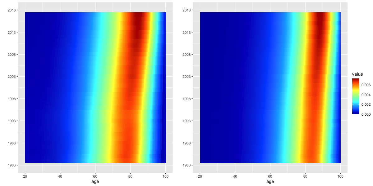
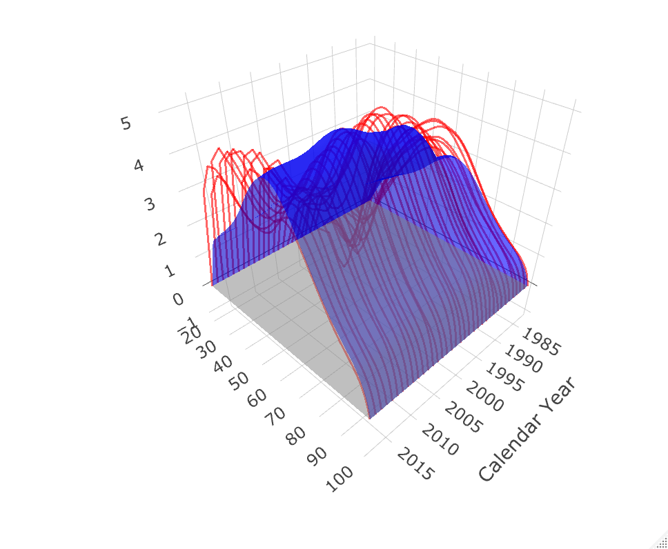
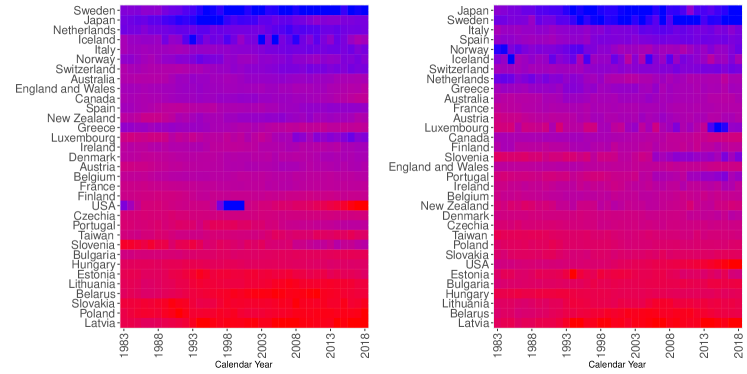
Human longevity has been actively studied over several decades and analyzing mortality data across countries and calendar years has provided key insights. The Human Mortality Database at www.mortality.org contains yearly age-at-death tables for 38 countries, grouped by age from 0 to 110+. Smooth densities of age-at-death distributions indexed by country and calendar year can be obtained by applying simple smoothing to the lifetables that are available in this database. We focused on the 33 countries for which data are available for the calendar years from 1983 to 2018. The distributions of age-at-death are viewed as an i.i.d. sample of distributional processes , where the index indicates the country and is calendar year. Using the Wasserstein metric , the Fréchet mean of the distributions for each calendar year in the form of densities indexed by calendar year is presented as heatmaps in Figure 2; the patterns of mortality for males and females are seen to differ substantially, as is well known.
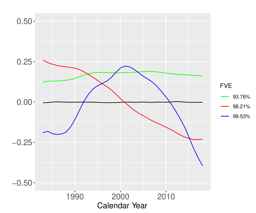
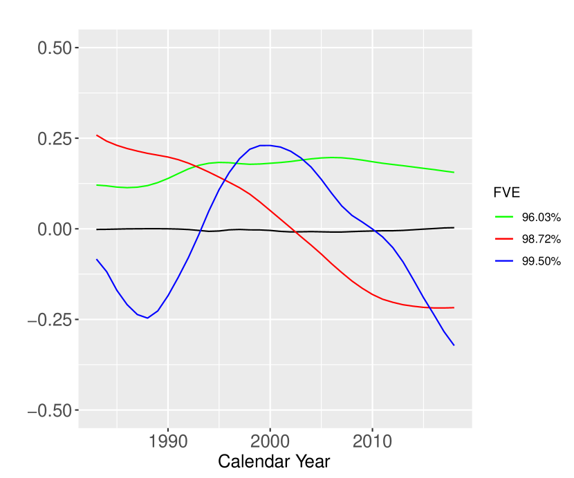
The optimal transports from to , denoted by , form the basis for our analysis. Figure 3 indicates that the estimated mean functions of the underlying processes that are defined in equation (11) are very close to 0, indicating there is no lack of fit. The first three eigenfunctions of the process for both males and females are shown in Figure 3. These eigenfunctions have similar patterns.
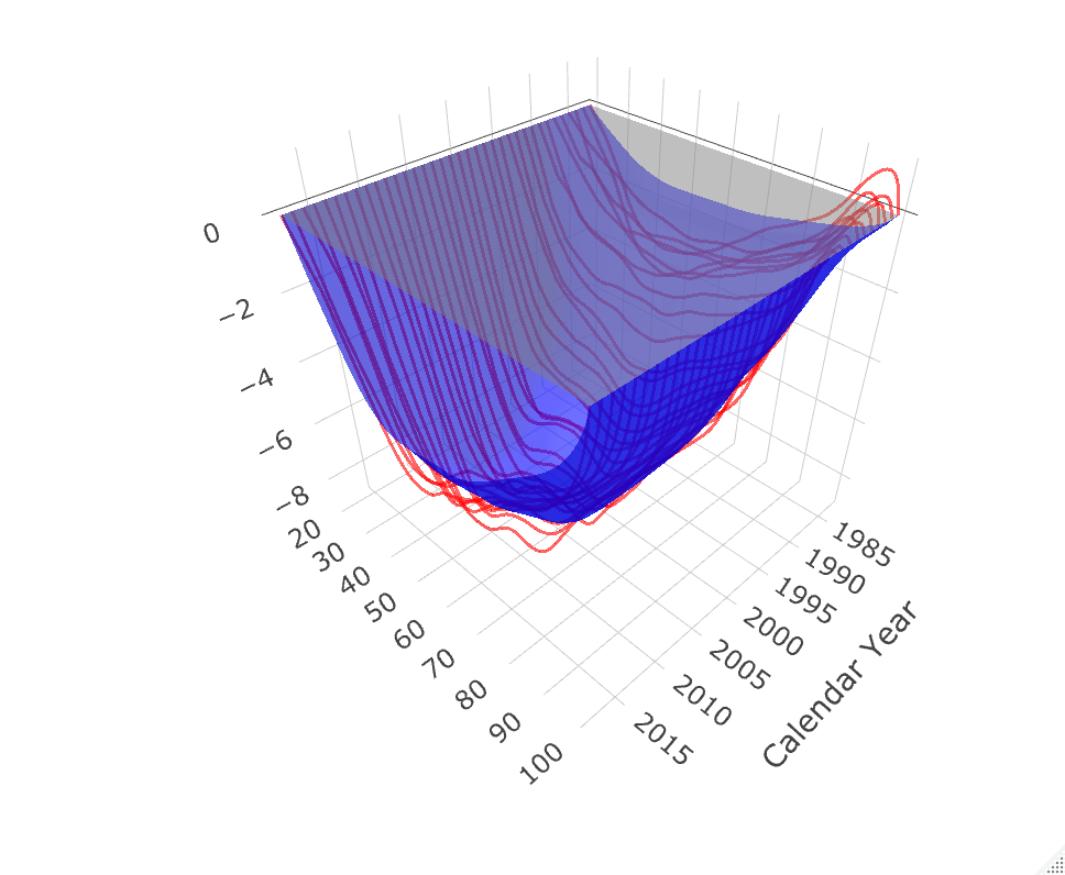
The representations obtained for two transport process trajectories utilizing the first three eigenfunctions of two randomly selected countries are shown in Figure 4, where we subtract the identity map for better illustration. The predicted processes are reasonably close to the data and are seen to provide good fits.
We also explored the sign changes of for each country. We found that for most of the richer countries, the signs of are positive, meaning that moves mass to the right from the Fréchet mean, associated with delayed age-at-death and increased longevity, while the with negative signs are primarily associated with lower income countries, where longevity is below average. But there are also interesting sign changes throughout the calendar period for various countries. Figure 5 shows the signs and the amount of mass that is transported to right or left.
7 Summary and discussion
Due to the rapid advancement of modern data collection technologies, non-Euclidean data have become increasingly prevalent. Over the past decade, the development of modeling object valued data has found increasing interest (Marron and Dryden, 2021). A key challenge in this context is the lack of linear structure, which plays an essential role in principal component analysis. A prevalent approach to surmount this obstacle involves mapping the data into linear spaces, however this remains unsatisfactory for maps that are isometric as then the inverse map is only defined on a subset of the image space; a typical example is local linearization with tangent bundles (Bigot et al., 2017; Chen et al., 2021). Direct linearizing transforms are generally invertible on the entire space (Petersen and Müller, 2016b) but are not isometric and lead to metric distortions. All of this makes intrinsic representations as we develop here attractive. We utilize the geodesic nature of the Wasserstein space to convert distribution-valued processes to transport processes, using transports in order to effectively subtract the barycenter of the process. This approach has two notable benefits. First, the transformation to transport processes is isometric, and we can equate the analysis of transport processes to that of distribution processes. Second, optimal transports naturally give rise to the centering operation for distribution-valued processes, effectively overcoming the absence of a subtraction operation. The transport processes are automatically centered and their mean is the identity process.
A central tenet of our proposed model is the decomposition of the time-varying transport process into a real-valued stochastic process and a random transport that characterizes the transport trajectory. This approach hinges on the reasonable assumption that the transport process exhibits a common pattern for all , with a specific pattern associated with each relaization. As demonstrated in Section 6, the proposed representation model and decomposition works well for real-world data. This decomposition is facilitated by the multiplication operation between a scalar and a transport map (Zhu and Müller, 2023a), leading to an equivalence relation within the transport space. Consequently, reside in an equivalence class, providing the geometric basis for the proposed representation. The stochastic process part in this decomposition introduces a real-valued stochastic process with ensuing eigenrepresentation. This is a major advantage as it means that one can bring to bear many concepts of functional data analysis, especially functional principal component analysis, in spite of the fact that there is no linear structure in the distribution space.
While the focus in this paper is on a single distribution process, a further advantage of considering transport processes is their capacity to model multivariate distribution processes. Specifically, in scenarios where constitute a pair of distributional trajectories and the relationship between these two components is of interest, one can consider optimal transports from to , which represent geodesics in the Wasserstein space. This connection adds to the appeal of transport processes. Furthermore, while we provide a detailed development here for the case of distribution-valued processes, this can serve as a blueprint for a larger class of metric-space valued processes in unique geodesic spaces where transports can be considered to move random objects along geodesics (Zhu and Müller, 2023b).
Appendix A Proofs and Auxiliary Results
A.1 Proofs of main results
We start by stating an important auxiliary result and its proof and then cover the proofs of the main results.
Proof 1 (Proof of Proposition 5).
Consider the probability space , where is a compact set of , is the Borel -algebra on and is a probability measure. The -valued functional data on is a measurable map, and is a Borel probability measure that generates the law of , i.e., for any Borel measurable .
For each and collection of , consider the valued random variable with probability measure
for Borel sets , where is the Borel -algebra generated by the open sets in . Suppose satisfies the following conditions:
-
(i)
for any permutation of ,
-
(ii)
for all , ,
Then by Kolmogorov’s extension theorem, there exists a unique probability measure on , the underlying law of the stochastic process , whose finite dimensional marginals are given by , whence is well defined.
Proof 2 (Proof of Theorem 1).
For the first statement in Theorem 1, we first show that
By definition,
where the last equality is due to on the set . Writing , we focus on the with only since by Lemma 2,
For ,
| (24) | ||||
For the first term in (24), note that is bounded for all ,
where the last inequality comes from Lemma 2. Note that
and
Thus, and for the second term on the right hand side of equation (24),
For ,
where the first inequality is due to the compactness of and the second inequality is from Lemma 2. Here is as in equation (1). For ,
Then the proof is completed by observing
Proof 3 (Proof of Theorem 2).
Next, we will derive the convergence rate for eigenfunctions and principal components scores. Note that and have the same eigenfunctions. By Bosq (2000) and Dubey and Müller (2020),
and
where . For the principal component scores, consider the convergence of ,
| (25) | ||||
For the first term on the right hand side of (25), by the compactness of ,
For the second term on the right hand side of (25), by Lemma 2,
For the third term on the right hand side of equation (25), by the central limit theorem
Thus
Next, we will show that
| (26) | ||||
Following the proof of Theorem 1,
Thus
whence
The second equation of (26) can be derived analogously.
Note that
| (27) | ||||
For the first term in equation (27),
| (28) | ||||
By equation (26), the first term on the right hand side of equation (28) is . Note that is bounded. The second term on the right hand side of (28) is bounded by
For the last term in equation (28),
Then the proof is complete since the second term in equation (27) can be bounded analogously.
Proof 4 (Proof of Theorem 3).
| (29) | ||||
as and defined in (20) and Corollary 1. To prove the first statement of Theorem 3, note that
| (30) | ||||
Under the assumptions for Lemma 1, we have
| (31) | ||||
where the last equality is from Lemma 1 and is finite.
For the first term on the right hand side of equation (30),
| (32) | ||||
where the second equality follows from Lemma 1 and the third equation of (31).
For the second term in equation (30), similarly
| (33) | ||||
For the third term in equation (30),
| (34) | ||||
where (a) follows from equation (39) and Lemma 2. This completes the proof of the first statement of Theorem 3.
For the second statement of Theorem 3, by (27) in the proof of Theorem 3, it is enough to consider the convergence rate of ,
| (35) | ||||
By equation (26) in the proof of Theorem 2, the first term on the right hand side of equation (35) is bounded by . For the second part, note that
Then the proof is completed by adopting similar arguments as in the proof of Theorem 2.
A.2 Proofs of auxiliary results and corollaries
Proof 5 (Proof of Proposition 2).
By the definition of , it is clear that and . We only need to show . First,
By the monotonicity of , we have on the set . Otherwise, there is , which is contradictory to . Thus
Analogously,
Thus
where the last equality is from Fubini’s Theorem. It is not hard to see that
for all or . For ,
Again by the monotonicity of , always has the same sign as . Thus,
Proof 6 (Proof of Proposition 3).
To show is a equivalence relation on , we need to check (i): for all ; (ii): implies for all ; (iii): If and then for all . Here (i) and (ii) are straightforward by the definition of , and we only need to check that transitivity holds. Given , we first assume there exists such that . If for , then and , thus . For the case , if , write then with . If , write then with . For the case , the argument is analogous.
It is worth noting that the binary relation : there exists such that or is not an equivalence relation on . To see this, let , and , which satisfy and . By calculation, one can get that , , and . When is positive, there does not exist any such that nor . When is negative, neither does there exist any such that nor . Thus, defined above is not an equivalence relation since it does not satisfy the transitivity property.
Proof 7 (Proof of Lemma 1).
For a given , consider the sequence space where
and its corresponding function space where
Note that , thus , which implies is larger than the general space. The definition of is related to a RKHS space and is a Hilbert space with the inner product and has an orthonormal basis .
Let denote the Dirac delta function, and . Under the assumption that the are uniformly bounded, we have for all . Let be the Dirac delta function centered on . Then it follows that the linear span is a subspace of . There is a map where
Clearly is a compact linear operator. Consider the matrix , where is the adjacent operator of . Then is a symmetric non-negative definite matrix and we denote its eigenvalues by . Since
and
where is the Riemann zeta function.
Our goal is to utilize the relation between and to recast the matrix as a product of operators. Consider the operator defined by
which is symmetric, positive definite and compact as long as as . We further have
| (36) |
To see this, by definition,
and
Then,
By equation (36), is non-negative definite, and we have , where and are the th eigenvalue and singular value of a matrix. The proof of Lemma 1 is complete if we show that . By the definition of , it is not hard to check and thus which is equivalent to for all . Under the assumption that are distinct, thus which implies that whence . Then implies , that is, .
Proof 8 (Proof of Lemma 2).
Without loss of generality, we assume the arguments are analogous for the cases where . Since , holds uniformly in for all . Note that
For the first term on the right hand side of the last equation, note that on the set one has
Thus,
where the last inequality follows from Assumption 3 and the convexity of on , and the last equality from Assumption 1. The proof is complete as was arbitrary.
Proof 9 (Proof of Corollary 1).
For the first statement of Corollary 1, by similar arguments as in Zhang and Wang (2016),
where for
with . Define
with .
To investigate the difference between and , write , and ,
| (37) | ||||
For the first term in equation (37), note that and are independent and is compact,
where the last inequality is based on
| (38) |
For the second term on the right hand side of equation (37), similarly,
From these relations, we get and thus
Noting that is uniformly bounded, by Theorem 4 and Corollary 1 in Zhou et al. (2022),
Then by similar arguments as in Zhang and Wang (2016), it is not hard to check that
and
For the second statement of Corollary 1, similarly,
with
where . Define
where . Using the definition of in (20), . Hence,
For ,
| (39) | ||||
where the last two inequalities rely on Assumption 4 and the rest of the proof is analogous to the above.
Proof 10 (Proof of Corollary 2 ).
When , the eigengap is and thus
By choosing the optimal bandwidth , we have
When , and the rate becomes . If , which implies . Then is minimized by choosing and the final rate becomes . Putting into the constraint gives and we get .
When , by choosing the optimal bandwidth,
When , and the rate becomes . If , is minimized at and the final rate becomes . Putting into the constraint , we get and the proof is complete.
Proof 11 (Proof of Corollary 3 ).
For the polynomial case, when and if , which implies , is minimized by choosing and the final rate is . Putting into the constraint , we get .
When , and the rate becomes
.
-
•
If , which implies , is minimized by choosing and the final rate is . Check that satisfies since and .
-
•
If , which implies
is minimized by choosing . However, putting into the constraint , we get , which contradicts to since for all .
For the exponential case, different from the polynomial case, the optimal is the solution of a transcendental equation for the case where is relatively small and is the dominating term. If , it is not hard to see that indeed is the dominating term and thus the rate becomes and is minimized at , which is the solution of the transcendental equation . Letting , it is not hard to see and has at most one zero point. Thus, and the proof is complete.
References
- Adler (1990) Adler, R. J. (1990). An introduction to continuity, extrema, and related topics for general gaussian processes. Lecture Notes-Monograph Series 12, i–155.
- Ambrosio et al. (2008) Ambrosio, L., N. Gigli, and G. Savaré (2008). Gradient Flows: in Metric Spaces and in the Space of Probability Measures. Springer Science & Business Media.
- Bigot et al. (2017) Bigot, J., R. Gouet, T. Klein, and A. López (2017). Geodesic PCA in the Wasserstein space by Convex PCA. Ann. inst. Henri Poincare (B) Probab. Stat. 53, 1–26.
- Bosq (2000) Bosq, D. (2000). Linear Processes in Function Spaces: Theory and Applications, Volume 149. Springer Science & Business Media.
- Cai and Yuan (2010) Cai, T. and M. Yuan (2010). Nonparametric covariance function estimation for functional and longitudinal data. University of Pennsylvania and Georgia inistitute of technology.
- Cai and Yuan (2011) Cai, T. T. and M. Yuan (2011). Optimal estimation of the mean function based on discretely sampled functional data: Phase transition. Ann. Statist. 39(5), 2330–2355.
- Chen et al. (2017) Chen, K., P. Delicado, and H.-G. Müller (2017). Modeling function-valued stochastic processes, with applications to fertility dynamics. J. R. Stat. Soc. Ser. B Stat. Methodol. 79, 177–196.
- Chen and Müller (2012) Chen, K. and H.-G. Müller (2012). Modeling repeated functional observations. J. Amer. Statist. Assoc. 107(500), 1599–1609.
- Chen et al. (2021) Chen, Y., P. Dubey, H.-G. Müller, M. Bruchhage, J.-L. Wang, and S. Deoni (2021). Modeling sparse longitudinal data in early neurodevelopment. NeuroImage 237, 118079.
- Chen et al. (2023) Chen, Y., Z. Lin, and H.-G. Müller (2023). Wasserstein regression. J. Amer. Statist. Assoc. 118(542), 869–882.
- Dai et al. (2021) Dai, X., Z. Lin, and H.-G. Müller (2021). Modeling sparse longitudinal data on riemannian manifolds. Biometrics 77(4), 1328–1341.
- Dai and Müller (2018) Dai, X. and H.-G. Müller (2018). Principal component analysis for functional data on Riemannian manifolds and spheres. Ann. Statist. 46(6B), 3334 – 3361.
- Dubey and Müller (2020) Dubey, P. and H.-G. Müller (2020). Functional models for time-varying random objects. J. R. Stat. Soc. Ser. B Stat. Methodol. 82(2), 275–327.
- Facer and Müller (2003) Facer, M. R. and H.-G. Müller (2003). Nonparametric estimation of the location of a maximum in a response surface. J. Multiv. Anal. 87(1), 191–217.
- Falk (1983) Falk, M. (1983). Relative efficiency and deficiency of kernel type estimators of smooth distribution functions. Stat. Neerl. 37(2), 73–83.
- Gangbo and McCann (1996) Gangbo, W. and R. J. McCann (1996). The geometry of optimal transportation. Acta Math. 177, 113–161.
- Ghodrati and Panaretos (2022) Ghodrati, L. and V. M. Panaretos (2022, 01). Distribution-on-distribution regression via optimal transport maps. Biometrika 109(4), 957–974.
- Hsing and Eubank (2015) Hsing, T. and R. Eubank (2015). Theoretical Foundations of Functional Data Analysis, with an Introduction to Linear Operators. John Wiley & Sons.
- Kokoszka et al. (2019) Kokoszka, P., H. Miao, A. Petersen, and H. L. Shang (2019). Forecasting of density functions with an application to cross-sectional and intraday returns. Int. J. Forecast. 35(4), 1304–1317.
- Kokoszka and Reimherr (2017) Kokoszka, P. and M. Reimherr (2017). Introduction to Functional Data Analysis. CRC press.
- Leblanc (2012) Leblanc, A. (2012). On estimating distribution functions using bernstein polynomials. Ann. Inst. Stat. Math. 64(5), 919–943.
- Li and Hsing (2010) Li, Y. and T. Hsing (2010). Uniform convergence rates for nonparametric regression and principal component analysis in functional/longitudinal data. Ann. Statist. 38(6), 3321–3351.
- Lin and Wang (2022) Lin, Z. and J.-L. Wang (2022). Mean and covariance estimation for functional snippets. J. Amer. Statist. Assoc. 117(537), 348–360.
- Lin and Yao (2019) Lin, Z. and F. Yao (2019). Intrinsic Riemannian functional data analysis. Ann. Statist. 47(6), 3533 – 3577.
- Marron and Dryden (2021) Marron, J. S. and I. L. Dryden (2021). Object Oriented Data Analysis. CRC Press.
- McCann (1997) McCann, R. J. (1997). A convexity principle for interacting gases. Adv. Math 128(1), 153–179.
- Panaretos and Zemel (2016) Panaretos, V. M. and Y. Zemel (2016). Amplitude and phase variation of point processes. Ann. Statist. 44(2), 771–812.
- Pegoraro and Beraha (2022) Pegoraro, M. and M. Beraha (2022). Projected statistical methods for distributional data on the real line with the Wasserstein metric. J. Mach. Learn. Res. 23, 37–1.
- Petersen et al. (2019) Petersen, A., C.-J. Chen, and H.-G. Müller (2019). Quantifying and visualizing intraregional connectivity in resting-state Functional Magnetic Resonance Imaging with correlation densities. Brain Connect. 9(1), 37–47.
- Petersen and Müller (2016a) Petersen, A. and H.-G. Müller (2016a). Fréchet integration and adaptive metric selection for interpretable covariances of multivariate functional data. Biometrika 103(1), 103–120.
- Petersen and Müller (2016b) Petersen, A. and H.-G. Müller (2016b). Functional data analysis for density functions by transformation to a hilbert space. Ann. Statist. 44(1), 183–218.
- Petersen et al. (2022) Petersen, A., C. Zhang, and P. Kokoszka (2022). Modeling probability density functions as data objects. Econom. Stat. 21, 159–178.
- Ramsay and Silverman (2006) Ramsay, J. and B. Silverman (2006). Functional Data Analysis. Springer Science & Business Media.
- Scealy and Welsh (2011) Scealy, J. and A. Welsh (2011). Regression for compositional data by using distributions defined on the hypersphere. J. R. Stat. Soc. Ser. B Stat. Methodol. 73(3), 351–375.
- Villani et al. (2009) Villani, C. et al. (2009). Optimal Transport: Old and New. Springer.
- Wang et al. (2016) Wang, J.-L., J.-M. Chiou, and H.-G. Müller (2016). Functional data analysis. Annu. Rev. Stat. Appl. 3, 257–295.
- Yao et al. (2005) Yao, F., H.-G. Müller, and J.-L. Wang (2005). Functional data analysis for sparse longitudinal data. J. Amer. Statist. Assoc. 100(470), 577–590.
- Zhang et al. (2022) Zhang, Q., B. Li, and L. Xue (2022). Nonlinear sufficient dimension reduction for distribution-on-distribution regression. arXiv preprint arXiv:2207.04613.
- Zhang and Wang (2016) Zhang, X. and J.-L. Wang (2016). From sparse to dense functional data and beyond. Ann. Statist. 44(5), 2281–2321.
- Zhou et al. (2021) Zhou, H., Z. Lin, and F. Yao (2021). Intrinsic wasserstein correlation analysis. arXiv preprint arXiv:2105.15000.
- Zhou et al. (2022) Zhou, H., D. Wei, and F. Yao (2022). Theory of functional principal components analysis for discretely observed data. arXiv preprint arXiv:2209.08768.
- Zhu and Müller (2023a) Zhu, C. and H.-G. Müller (2023a). Autoregressive optimal transport models. J. R. Stat. Soc. Ser. B Stat. Methodol. 85(3), 1012–1033.
- Zhu and Müller (2023b) Zhu, C. and H.-G. Müller (2023b). Spherical autoregressive models, with application to distributional and compositional time series. Journal of Econometrics.