Electron Interactions in Rashba Materials

Abstract

We show that Rashba spin-orbit interaction (RSOI) modifies electron-electron interaction vertex giving rise to a spectrum of novel phenomena. First, the spin-orbit-modified Coulomb interactions induce $p$-wave superconducting order, without any need for other mediators of attraction. Remarkably, two distinct superconducting phases arise in 3D systems, mirroring the A or B phases of ³He, depending on the sign of the SOI constant. In contrast, 2D systems exhibit $p^{x}\pm ip^{y}$ order parameter, leading to time-reversal-invariant topological superconductivity. Second, a sufficiently strong RSOI induces ferromagnetic ordering. It is associated with a deformation of the Fermi surface, which may lead to a Lifshitz transition from a spherical to a toroidal Fermi surface, with a number of experimentally observable signatures. Finally, in sufficiently clean Rashba materials, ferromagnetism and $p$-wave superconductivity may coexist. This state resembles the A₁ phase of ³He, yet it may avoid nodal points due to the toroidal shape of the Fermi surface.

I Introduction

The study of spin-orbit interaction has been a fascinating area of research in condensed matter physics for several decades [1, 2, 3]. Rashba spin-orbit interaction (RSOI) offers a new way to control spin states using purely electrical means rather than magnetic fields. This presents a massive advantage for spintronics, a field of study that aims to exploit the quantum spin degree of freedom [4, 5] to develop new computational and data storage technologies [6, 7, 8].

In recent years, the discovery of materials with giant RSOI has opened up new avenues for investigating exotic quantum phenomena and exploring potential applications in spintronic devices [9, 10, 11, 12, 13, 14, 15, 16]. These include the engineered $\mathrm{LaAlO_{3}/SrTiO_{3}}$ heterostructures [17, 18, 19, 20] and graphene on the two-dimensional (2D) layers of the transition metal dichalcogenides [21, 22, 23], to name a few.

The Rashba effect [24], characterized by locking of spin and momenta directions, results in lifting the spin-degeneracy of conduction band electrons away from the center of a Brillouin zone. While RSOI may occur from the structure inversion asymmetry, in the present paper we focus exclusively on the extrinsic RSOI, produced by electric fields external to the crystalline lattice. Extrinsic RSOI arises due to the non-commutativity of the extrinsic electric potential with the intrinsic Hamiltonian of the host crystal [25]. On a more formal level, it originates from a momentum dependent Berry phase, emerging due to a mixing between the conduction and valence bands. If the valence bands are split by intra-atomic relativistic SOI, the Berry phase acquires a spin-dependent component, which gives rise to RSOI.

The origin of the Berry phase lies in the non-commutativity of a momentum-dependent unitary transformation, $U({\bm{p}})$, from atomic orbitals to Bloch bands basis and a coordinate-dependent scalar potential, $\varphi({\bm{r}})$. The Moyal expansion of these non-commutative operators leads to gradient commutators of the form $\varepsilon_{\lambda\mu\nu}\grad^{\nu}_{\bm{r}}\varphi({\bm{r}})\grad^{\mu}_{\bm{p}}U(\bm{p})\,\hat{\sigma}^{\lambda}$, where $\mu,\nu,\lambda$ are Cartesian coordinates and $\hat{\sigma}$ are spin Pauli matrices. In this way Rashba spin-orbit effects are inextricably proportional to an extrinsic electric field $\bm{\mathcal{E}}(\bm{r})=-\bm{\nabla}_{\!\bm{r}}\varphi({\bm{r}})$.

For conduction band electrons close to the Brillouin zone center the resulting coupling can be described via a commonly used phenomenological single-particle Rashba Hamiltonian, which is linear in the wave vector, $\bm{p}$, [26]

$$H=\alpha\left[\bm{\mathcal{E}}\times{\bm{p}}\right]\cdot\hat{\bm{\sigma}},$$ (1)

where $\alpha$ is a material-dependent Rashba constant. In 2D systems, the extrinsic electric field, $\bm{\mathcal{E}}$, can originate from external factors such as gate voltages. In contrast, in 3D metallic crystals, the uniform electric fields are typically screened. However, the local fields can emerge due to charged impurities and structural defects [27, 28]. These local extrinsic fields contribute to a wide range of phenomena, notably the anomalous Hall and spin Hall effects [29, 30, 31, 32, 33].

An advent of pair spin-orbit interactions (PSOI) [34] comes from a simple realization that the electric field, $\bm{\mathcal{E}}$, in Eq. (1) may equally well come from the Coulomb electron-electron interactions. We emphasize that no inversion symmetry breaking is required for PSOI effects. Accepting this fact immediately leads to a number of remarkable consequences.

The emerging spin order is qualitatively different from the more familiar single-particle RSOI. Take, e.g., a 2D case: the normal electric field of the single-particle RSOI (1) results in a chiral locking of in-plane spins and momenta. On the other hand, for the PSOI the electric field (as well as momentum) are purely in-plane, forcing spins to be ordered along the normal direction. Despite their potential to give rise to intriguing collective phenomena [35], manifestations of the Rashba effect in the two-body interactions remain relatively unexplored.

The PSOI is capable of triggering instabilities in the charge sector of 1D and 2D electron systems. These instabilities in the particle-particle channel may facilitate formation of bound electron pairs with non-trivial orbital and spin structure, including $p$-wave pairing [36, 37, 38, 39, 40, 41, 42]. Furthermore, the instabilities observed in the particle-hole channel act as a precursor for phase separation, assisting the development of highly unconventional correlated states [43, 44, 45].

In this work, we focus on superconducting and magnetic instabilities in 3D and 2D Rashba materials [46, 47]. The former manifests itself in a particular $p$-wave superconducting state, which in 3D may be nodal or node-less depending on the sign of the SOI constant, $\alpha$. The order parameters of these two superconducting phases mirror those of the A and B phases in ³He [48], revealing surprising parallels between these two distinct systems.

In 2D systems, the $p$-wave superconducting states are fully gapped, pairing spin up/down electrons into $p^{x}\pm ip^{y}$ states. Notably, the superconducting state in 2D is topological and maintains time-reversal symmetry [49]. In the strongly coupled regime, this superconducting state can be viewed as the Bose-Einstein condensate of the electron pairs bound by PSOI, which were previously explored in the literature [36, 37, 38, 39, 40]. However, the instability in the $p$-wave Cooper channel occurs already for a weak PSOI as a first order effect in the interaction strength. Remarkably, the stability of such superconducting states does not require phonons or any others mediators of attraction, and relies solely on the interplay between screened Coulomb repulsion and PSOI. It does impose, however, certain requirements on the purity of the material.

The ferromagnetic (FM) ordering comes from the Stoner-like mechanism for a sufficiently large SOI constant, $\alpha$. Due to PSOI the FM breaking of the rotation symmetry in the spin space is associated with a deformation and eventual topology-changing Lifshitz transition of the Fermi surface in the momentum space. Such a transition from genus-zero to genus-one Fermi surface leads to experimentally detectable consequences in thermodynamic and transport properties, as well as in spectra of Shubnikov-de Haas and Friedel oscillations. Finally, the FM and the $p$-wave superconducting orders may coexist. Interestingly, the toroidal Fermi surface allows for a node-less fully spin-polarized order parameter for either sign of $\alpha$.

II Electron-electron interactions in Rashba Materials

In this section we work out consequences of the phenomenological Rashba spin-orbit coupling, Eq. (1), for electron-electron interaction Hamiltonian. To this end consider a 3D Rashba system without the inversion symmetry breaking. A 2D case is a simple particular case of this consideration, which is briefly mentioned in the end. We do not consider the effects of disorder in our analysis. Furthermore, since a bulk electric field is not allowed in a 3D electronic system, it might be tempting to conclude that the Rashba spin-orbit interaction term, as given in Eq. (1), is inconsequential. However, such conclusion is premature because of the fluctuating electric fields created by electron-electron interactions.

To describe the physics originating from this observation one deals with a two-component spinor electron creation operator $\hat{\psi}_{\bm{p}}^{\dagger}\equiv\spinor{\hat{c}_{\bm{p},\uparrow}^{\dagger}\hat{c}_{\bm{p},\downarrow}^{\dagger}}$, describing conduction band electrons in a spin-up/spin-down basis. The corresponding electron creation operator in the coordinate basis is denoted as $\hat{\psi}^{\dagger}(\bm{r})$.

It is convenient to define the spin current tensor as

$$\hat{\jmath}^{\lambda\mu}(\bm{r})=\frac{1}{2mi}\left(\hat{\psi}^{\dagger}(\bm{r})\hat{\sigma}^{\lambda}\grad_{\bm{r}}^{\mu}{\hat{\psi}(\bm{r})}-(\grad_{\bm{r}}^{\mu}{\hat{\psi}^{\dagger}(\bm{r})})\hat{\sigma}^{\lambda}\hat{\psi}(\bm{r})\right),$$ (2)

with Greek indices $\lambda,\mu,\ldots$ standing for the Cartesian components.  This object describes a flow of the $\lambda$ component of the spin angular momentum in the $\mu$ spatial direction. The Hamiltonian for electrons interacting with an external scalar electric potential, $\varphi(\bm{r},t)$, which includes RSOI, Eq. (1), is

$$\begin{split}\hat{H}_{\mathrm{ext}}&=-\int d\bm{r}\,\left(e\varphi(\bm{r},t)\hat{\rho}(\bm{r})+\alpha m\,\varepsilon_{\lambda\mu\nu}\mathcal{E}^{\nu}(\bm{r})\hat{\jmath}^{\lambda\mu}(\bm{r})\right)\\ &=-\int d\bm{r}\,\varphi(\bm{r},t)\left(e\hat{\rho}(\bm{r})+\alpha m\,\varepsilon_{\lambda\mu\nu}\grad_{\bm{r}}^{\nu}\hat{\jmath}^{\lambda\mu}(\bm{r})\right)\\ &=-\int d\bm{r}\,\varphi(\bm{r},t)\left(e\hat{\psi}^{\dagger}\hat{\psi}+i\alpha\,\varepsilon_{\lambda\mu\nu}\grad_{\bm{r}}^{\mu}\hat{\psi}^{\dagger}\hat{\sigma}^{\lambda}\grad_{\bm{r}}^{\nu}\hat{\psi}\right),\end{split}$$ (3)

where $\hat{\rho}(\bm{r})\equiv\hat{\psi}^{\dagger}(\bm{r})\hat{\psi}(\bm{r})$ is the electron density, and $\varepsilon_{\lambda\mu\nu}$ is the Levi-Civita symbol. In the second line we used that $\mathcal{E}^{\nu}(\bm{r})=-\grad_{\bm{r}}^{\nu}\varphi(\bm{r})$ and performed integration by parts. The last terms in the integrands here are the RSOI. It can be viewed as the spin-dependent renormalization of the electron density operator by the gradient corrections. Its appearance warrants some elaboration. The very notion of the SOI is an attribute of a simplified single-band portrayal of the electron dynamics, accomplished via the projection of a microscopic multi-band Hamiltonian onto the conduction band. Through this projection, an effective Hamiltonian emerges with the SOI term, reflecting the contribution of the valence band(s) to the conduction band electrons dynamics. In particular, the local scalar potential disturbs both valence and conduction bands. Due to the momentum-dependent nature of the rotation from local orbitals to the band representation, it leads to the gradient correction to the conduction-band density response. The SOI term in Eq. (3) reflects the spin-dependent part of this gradient correction. The $\sim\hat{\sigma}_{0}$ gradient terms may also exist, but they do not lead to qualitatively new effects.

One can be excused to think that the sign of the SOI strength, $\alpha$, in Eq. (3) does not have a physical significance since the change of $\alpha\to-\alpha$ may be compensated by $\bm{\sigma}\to-\bm{\sigma}$ transformation. Yet this logic is erroneous, since $\bm{\sigma}\to-\bm{\sigma}$ is not a faithful representation of $\uparrow\leftrightarrow\downarrow$ exchange. Indeed, consider $\hat{\psi}^{\dagger}\hat{\sigma}^{\lambda}\hat{\psi}$ combination. While for $\lambda=y,z$ one indeed observes that $\uparrow\leftrightarrow\downarrow$ is equivalent to $\sigma^{y,z}\to-\sigma^{y,z}$, this logic does not work for $\lambda=x$. Therefore, if all three Pauli matrices are employed (as in 3D case), $\bm{\sigma}\to-\bm{\sigma}$ is not a legitimate transformation and a sign of $\alpha$ does have physical significance. On the other hand, if SOI term is somehow limited to two Pauli’s (like in 2D, where $\lambda=z$ in Eq. (3), or $\lambda=x,y$ in Eq. (1)), the physical observables are invariant with respect to $\alpha\to-\alpha$.

Throughout the text, $e\equiv\lvert q_{e}\rvert>0$ stands for the absolute value of the electron charge $q_{e}$. In the notations of Eq. (1), the SOI constant $\alpha$ is positive for the electrons in vacuum, $\alpha=e\lambdabar_{C}^{2}/4$, with $\lambdabar_{C}$ being the Compton wavelength. Within the Kane $8\times 8$ model of the semiconductor band structure [50], the SOI constant is given by [51, 26]

$$\alpha=\frac{eP^{2}}{3}\left[\frac{1}{{(E_{0}+\Delta_{SO})}^{2}}-\frac{1}{E_{0}^{2}}\right]\,,$$ (4)

with the energy gap $E_{0}$, the energy of the split-off holes $\Delta_{SO}$, and the dipole matrix element $P$. For $\Delta_{SO}>0$, the SOI magnitude, $\alpha$, is negative, i.e. has the sign opposite to that in the vacuum [25]. The actual sign of the Rashba SOI in realistic structures depends on a particular charge asymmetry near the atomic cores [52], which may affect e.g. the spin texture of the electron state [53, 54].

In the momentum representation Eq. (3) results in the following interaction vertex between the electrons and the scalar potential

$$\hat{H}_{\mathrm{ext}}=\sum_{\bm{p}_{1},\bm{p}_{2}}\varphi(\bm{p}_{2}-\bm{p}_{1},t)\,\hat{\psi}^{\dagger}_{\bm{p}_{1}}\hat{\Gamma}_{\bm{p}_{1}\bm{p}_{2}}\hat{\psi}_{\bm{p}_{2}}\,,$$ (5)

where the vertex $\hat{\Gamma}_{\bm{p}_{1}\bm{p}_{2}}$ is a matrix in the spin as well as in the momentum spaces given by 

$$\hat{\Gamma}_{\bm{p}_{1}\bm{p}_{2}}=-e\hat{\sigma}_{0}-i\alpha_{p_{1}p_{2}}[\bm{p}_{1}\times\bm{p}_{2}]\cdot\hat{\bm{\sigma}}\,.$$ (6)

In writing this expression, we accommodated the possibility that the SOI “constant”, $\alpha$, can in fact exhibit momentum dependence, $\alpha\to\alpha_{p_{1}p_{2}}$, making $\alpha_{p_{1}p_{2}}$ to decrease if either of the two momenta exceeds a certain cutoff. Such dependence indeed arises from a more detailed microscopic analysis within a multi-band model, as outlined in Appendix A.

In interacting systems the scalar potential is a quantized Gaussian fluctuating field with the correlation function given by $\langle\varphi(\bm{q},t)\varphi(-\bm{q},t^{\prime})\rangle\equiv\mathcal{U}_{\bm{q}}\,\delta(t-t^{\prime})$. In 3D materials the latter is the usual Coulomb potential, $\mathcal{U}_{\bm{q}}=4\pi/q^{2}$, while in 2D it may include effects of dielectric constant $\epsilon$ of a surrounding media and, possibly, screening by external metallic gates. This leads to the e-e interaction Hamiltonian of the form:

$$\hat{H}_{\mathrm{int}}=\frac{1}{2}\sum_{\begin{subarray}{c}\bm{p}_{1},\bm{p}_{2}\\ \bm{p}^{\prime}_{1},\bm{p}^{\prime}_{2}\end{subarray}}\mathcal{U}_{\bm{p}_{2}-\bm{p}_{1}}\!\normord{\hat{\psi}^{\dagger}_{\bm{p}_{1}}\hat{\Gamma}_{\bm{p}_{1}\bm{p}_{2}}\hat{\psi}_{\bm{p}_{2}}\hat{\psi}^{\dagger}_{\bm{p}^{\prime}_{1}}\hat{\Gamma}_{\bm{p}^{\prime}_{1}\bm{p}^{\prime}_{2}}\hat{\psi}_{\bm{p}^{\prime}_{2}}}\,,$$ (7)

where the momentum summation is limited to momentum conserving processes with $\bm{p}_{1}+\bm{p}^{\prime}_{1}=\bm{p}_{2}+\bm{p}^{\prime}_{2}$ and the colon signs denote the normal ordering of the electron creation/annihilation operators.

The total Hamiltonian $\hat{H}_{\mathrm{tot}}=\hat{H}_{\mathrm{kin}}+\hat{H}_{\mathrm{int}}$ also includes the kinetic energy

$$\hat{H}_{\mathrm{kin}}=\sum_{\bm{p}}\hat{\psi}^{\dagger}_{\bm{p}}\,\xi_{\bm{p}}\hat{\sigma}_{0}\,\hat{\psi}_{\bm{p}}\,.$$ (8)

To be specific, we assume quadratic energy dispersion, $\xi_{\bm{p}}=\bm{p}^{2}/2m-\mu$.

In 2D systems, one may also take into account the one-body RSOI produced by the normal electric field $\mathcal{E}_{z}$ of the gate. In this case, the single-particle Hamiltonian is

$$\hat{H}_{\mathrm{kin}}=\sum_{\bm{p}}\hat{\psi}^{\dagger}_{\bm{p}}\left(\xi_{\bm{p}}\hat{\sigma}_{0}+\alpha\,\mathcal{E}_{z}{[\bm{p}\times\hat{\bm{\sigma}}]}_{z}\right)\hat{\psi}_{\bm{p}}\,,$$ (9)

where both $\bm{p}$ and $\hat{\sigma}$ are 2D vectors in $x-y$ plane. The corresponding interaction vertex acquires the spin-diagonal form: $\hat{\Gamma}_{\bm{p}_{1}\bm{p}_{2}}=-e\hat{\sigma}_{0}-i\alpha_{p_{1}p_{2}}{[\bm{p}_{1}\times\bm{p}_{2}]}_{z}\hat{{\sigma}}_{z}$, as both the initial and final momenta are in the $x-y$ plane.

III $P$-wave Superconductivity

Here, we show that the interplay of PSOI and Coulomb repulsion favors $p$-wave superconducting order, circumventing the need for phonons or other mediators of attraction. The mechanism bears similarities to the Kohn-Luttinger higher angular momentum superconductivity [55, 56]. The key distinction lies in the source of the effective attraction in odd orbital channels. In the present case it originates from the PSOI, while the interaction potential, $\mathcal{U}_{\bm{q}}$, may be considered as a structureless short-range potential (either repulsive or attractive). Notably, our mechanism is a direct, first-order effect in the interaction strength, distinguishing it from the Kohn-Luttinger scenario that arises as a higher-order effect — second order in 3D and third order in 2D [57].

III.1 Variational Considerations

Consider an approximate Bardeen–Cooper–Schrieffer (BCS) Hamiltonian that describes the pairing interaction between electrons with zero total momentum. Making the spin indexes explicit, the interaction Hamiltonian (7) acquires the form

$$\hat{H}_{\mathrm{BCS}}\propto\mathcal{U}_{\bm{p}_{2}-\bm{p}_{1}}\hat{\Gamma}_{\bm{p}_{1}\bm{p}_{2}}^{s_{1}s_{2}}\hat{\Gamma}_{-\bm{p}_{1}-\bm{p}_{2}}^{r_{1}r_{2}}\,{\psi}^{\dagger}_{\bm{p}_{1}s_{1}}{\psi}^{\dagger}_{-\bm{p}_{1}r_{1}}{\psi}_{-\bm{p}_{2}r_{2}}{\psi}_{\bm{p}_{2}s_{2}},$$ (10)

where we omitted momentum and spin summation symbols for brevity. Anticipating the spin-triplet superconductivity, we introduce the anomalous expectation value as a symmetric complex matrix in the spin space:

$$\hat{d}^{\,rs}_{\bm{p}}\!=\left\langle{\psi}_{-\bm{p}r}{\psi}_{\bm{p}s}\right\rangle=\!\begin{pmatrix}-d^{x}_{\bm{p}}+id^{y}_{\bm{p}}&d^{z}_{\bm{p}}\\ d^{z}_{\bm{p}}&\!\!\!\!d^{x}_{\bm{p}}+id^{y}_{\bm{p}}\end{pmatrix}\!=\bm{d}_{\bm{p}}\cdot{(\bm{\hat{\sigma}}\,i\hat{\sigma}_{y})}_{rs}\,,$$ (11)

where the complex vector $\bm{d}_{\bm{p}}$ is an odd function of the orbital momentum:

$$\bm{d}_{-\bm{p}}=-\bm{d}_{\bm{p}}\,.$$ (12)

As follows from Eq. (11), $\mp d^{x}_{\bm{p}}+id^{y}_{\bm{p}}$ describe $m=\pm 1$ components of the triplet order parameter, while $d^{z}_{\bm{p}}$ is its $m=0$ component. Here $m$ labels projections of the $l=1$ spin angular momentum.

The anomalous averages (11) result in the following expectation value of the BCS Hamiltonian (10):

$$\langle\hat{H}_{\mathrm{BCS}}\rangle\!\propto\!\mathcal{U}_{\bm{p}_{2}-\bm{p}_{1}}\!\!\operatorname{Tr}\!\left\{\!(-i\hat{\sigma}_{y}\bm{\hat{\sigma}})\!\cdot\!\bar{\bm{d}}_{\bm{p}_{1}}\hat{\Gamma}_{\bm{p}_{1}\bm{p}_{2}}\bm{d}_{\bm{p}_{2}}\!\cdot\!(\bm{\hat{\sigma}}\,i\hat{\sigma}_{y})\hat{\Gamma}_{\bm{p}_{1}\bm{p}_{2}}^{\intercal}\!\right\},$$ (13)

where the trace and matrix transposition are performed in the spin space only, and we used that $\hat{\Gamma}_{-\bm{p}_{1}-\bm{p}_{2}}=\hat{\Gamma}_{\bm{p}_{1}\bm{p}_{2}}$. Employing that $\hat{\sigma}_{y}{(\hat{\sigma}^{\lambda})}^{\intercal}\hat{\sigma}_{y}=-\hat{\sigma}^{\lambda}$ and

$$\operatorname{Tr}\left\{{\hat{\sigma}}^{\mu}{\hat{\sigma}}^{\nu}\right\}=2\delta^{\mu\nu};\qquad\operatorname{Tr}\left\{{\hat{\sigma}}^{\mu}\hat{\sigma}^{\lambda}{\hat{\sigma}}^{\nu}\right\}=2i\varepsilon^{\mu\lambda\nu};$$

$$\operatorname{Tr}\left\{{\hat{\sigma}}^{\mu}\hat{\sigma}^{\lambda}{\hat{\sigma}}^{\nu}\hat{\sigma}^{\gamma}\right\}=2\left(\delta^{\mu\lambda}\delta^{\nu\gamma}-\delta^{\mu\nu}\delta^{\lambda\gamma}+\delta^{\mu\gamma}\delta^{\lambda\nu}\right)\,,$$

one obtains

$$\begin{split}\left\langle\hat{H}_{\mathrm{BCS}}\right\rangle={}&2\!\sum_{\bm{p}_{1},\bm{p}_{2}}\mathcal{U}_{\bm{p}_{2}-\bm{p}_{1}}\big{\{}e^{2}(\bar{\bm{d}}_{\bm{p}_{1}}\!\cdot\bm{d}_{\bm{p}_{2}})\\ &{}+2e\alpha\,[\bar{\bm{d}}_{\bm{p}_{1}}\!\times\bm{d}_{\bm{p}_{2}}]\cdot[\bm{p}_{1}\!\times\bm{p}_{2}]\\ &{}+2\alpha^{2}(\bar{\bm{d}}_{\bm{p}_{1}}\!\cdot[\bm{p}_{1}\!\times\bm{p}_{2}])([\bm{p}_{1}\!\times\bm{p}_{2}]\!\cdot{\bm{d}}_{\bm{p}_{2}})\\ &{}-\alpha^{2}(\bar{\bm{d}}_{\bm{p}_{1}}\!\cdot\bm{d}_{\bm{p}_{2}})\left\lvert[\bm{p}_{1}\!\times\bm{p}_{2}]\right\rvert^{2}\big{\}}\,.\end{split}$$ (14)

To simplify discussion of Eq. (14) let us first assume short range repulsive interaction (e.g., screened Coulomb) with $\mathcal{U}_{\bm{p}_{2}-\bm{p}_{1}}=\mathcal{U}_{0}>0$. This may seem to be in contradiction with the announced $p$-wave nature of the anomalous averages. Indeed, being taken at the same spatial point the triplet component (11) seems to be zero. This is not the case due to the spin-orbit part of the interactions, which adds factors $[\bm{p}_{1}\times\bm{p}_{2}]$ to the interaction vertexes. This makes the effective interaction to be momentum-dependent, even if $\mathcal{U}_{\bm{p}_{2}-\bm{p}_{1}}=\operatorname{const}$. In other words, factors $[\bm{p}_{1}\times\bm{p}_{2}]$ mean derivatives of the $\psi$ operators in Eq. (11): $\langle\grad^{\mu}\hat{\psi}\grad^{\nu}\hat{\psi}\rangle$, cf. Eq. (3), which does not have to vanish, even if taken at the same spatial point.

With this assumption, due to the odd character of $\bm{d}_{\bm{p}}$, only linear in the spin-orbit magnitude, $\alpha$, term contributes to the BCS energy (14)

$$\left\langle\hat{H}_{\mathrm{BCS}}\right\rangle=4e\alpha\mathcal{U}_{0}\!\sum\limits_{\bm{p}_{1},\bm{p}_{2}}[\,\bar{\bm{d}}_{\bm{p}_{1}}\!\times\bm{d}_{\bm{p}_{2}}]\cdot[\bm{p}_{1}\!\times\bm{p}_{2}].$$ (15)

This form of the BCS energy suggests to introduce tensorial local order parameter

$$D^{\nu\nu^{\prime}}=\sum_{\bm{p}}{d}_{\bm{p}}^{\,\nu}\,{p}^{\nu^{\prime}}=\tfrac{1}{2}{(-i\hat{\sigma}_{y}\hat{\sigma}^{\nu})}_{sr}\left\langle{\psi}_{r}(\bm{r})i\nabla_{\bm{r}}^{\nu^{\prime}}{\psi}_{s}(\bm{r})\right\rangle\,.$$ (16)

Notice that the odd character of $\bm{d}_{\bm{p}}$, Eq. (12), is crucial for this definition to make sense. In terms of this quantity the BCS energy (15) becomes a quadratic form:

$$\left\langle\hat{H}_{\mathrm{BCS}}\right\rangle=4e\alpha\mathcal{U}_{0}\,\,\bar{D}^{\mu\mu^{\prime}}T^{\mu\mu^{\prime},\nu\nu^{\prime}}D^{\nu\nu^{\prime}}\,,$$ (17)

labelled by the 9-component index $\nu\nu^{\prime}=(xx,xy,\ldots,zz)$. The symmetric $9\times 9$ matrix is $T^{\mu\mu^{\prime},\nu\nu^{\prime}}=\sum_{\lambda}\varepsilon^{\mu\nu\lambda}\varepsilon^{\mu^{\prime}\nu^{\prime}\lambda}$. Its eigenvalues are

$$\left\{2,1,1,1,-1,-1,-1,-1,-1\right\}\,.$$ (18)

The fact that there are both positive and negative eigenvalues, means that for any sign of $e\alpha\mathcal{U}_{0}$ the system is unstable against development of a triplet superconducting order. However the character of this instability depends on the sign of $e\alpha\mathcal{U}_{0}$. This illustrates that in 3D the sign of $e\alpha$ has a physical meaning and there is no invariance with respect to $\alpha\to-\alpha$ transformation, similar to quasi-2D systems with non-zero curvature [58]. Notice that in flat 2D systems the situation is different: in this case both $\nu$ and $\nu^{\prime}$ are confined to the $x,y$ plane and thus so are $\mu,\mu^{\prime}$. This confines the quadratic form to be a $4\times 4$ matrix, $T^{\mu\mu^{\prime},\nu\nu^{\prime}}=\varepsilon^{\mu\nu z}\varepsilon^{\mu^{\prime}\nu^{\prime}z}$, with a symmetric spectrum $\{1,1,-1,-1\}$. This reflects the fact that in 2D the combined $\alpha\to-\alpha$ and up $\to$ down transformations is the symmetry of the Rashba Hamiltonian.

For $e\alpha\mathcal{U}_{0}<0$, which for repulsive interactions corresponds to $\alpha<0$, the most unstable direction is associated with the eigenvalue $2$ of the $T^{\mu\mu^{\prime},\nu\nu^{\prime}}$ form. The corresponding eigenvector has equal components in $xx,yy$, and $zz$ directions. This corresponds to the isotropic $p$-wave order parameter with $\bm{d}_{\bm{p}}\propto\bm{p}$. As shown in the next section, it leads to a node-less state with a gap isotropic around the Fermi surface. Such state is similar to the B phase of superfluid ³He [48]. For $e\alpha\mathcal{U}_{0}>0$ there are five degenerate unstable directions, corresponding to the eigenvalue $-1$. All of them break the rotational symmetry and lead to a nodal order parameter. One representative unstable direction is given by $\bm{d}_{\bm{p}}\propto(p^{x},-p^{y},0)$. We will show that it results in $p^{x}\pm ip^{y}$ order parameters for up/down spin components with nodes along the $p^{z}$-direction. This state is similar to the A phase of ³He [48].

To investigate limitations of the short-range interactions results, we consider a screened Coulomb interaction potential in the Thomas-Fermi (i.e. static, long-wavelength) approximation, $\mathcal{U}_{\bm{q}}=4\pi/(q^{2}+\kappa^{2})$, where $\kappa=\sqrt{4\pi e^{2}\nu_{3}}$ is the inverse Thomas-Fermi screening radius, with $\nu_{d}$ standing for the density of states at the Fermi energy in dimension $d=2,3$. We then substitute such an interaction potential and the isotropic order parameter, $\bm{d}_{\bm{p}}\propto\bm{p}$, into the variational energy (14) and look when the latter is negative. Performing somewhat tedious but straightforward angular integrals and putting $p_{1}\approx p_{2}\approx p_{F}$, one finds the condition for the isotropic (i.e. occurring at $\alpha<0$) $p$-wave instability:

$$\frac{\lvert\alpha\rvert\,p_{F}^{2}}{e}>f\left(\frac{p_{F}}{\kappa}\right)\,,$$ (19)

where the positive function $f$ is $f(x)\approx x^{2}/2$ for $x\ll 1$ and $f(x)\approx\sqrt{3\log x}\,$ for $x\gg 1$. A similar calculation may be done for $\alpha>0$ and the anisotropic order. The simplified take-home message is that the condition for the $p$-wave instability is

$$\lvert\alpha\rvert\max\{\kappa^{2},p_{F}^{2}\}\gtrsim e\,.$$ (20)

III.2 Self-Consistency Condition

To figure out the fate of the $p$-wave instability, explained above, we formulate $4\times 4$ Bogoliubov-de-Gennes (BdG) Hamiltonian in the Nambu times spin space. In the basis where $\bar{\Psi}_{\bm{p}}=(\bar{\psi}_{\bm{p}\uparrow},\bar{\psi}_{\bm{p}\downarrow},\psi_{-\bm{p}\uparrow},\psi_{-\bm{p}\downarrow})$, it takes the form:

$$\hat{H}_{\mathrm{BdG}}=\sum_{\bm{p}}\,\bar{\Psi}_{\bm{p}}\begin{pmatrix}\xi_{\bm{p}}\hat{\sigma}_{0}&\hat{\Delta}_{\bm{p}}\\ \hat{\Delta}_{\bm{p}}^{\dagger}&-\xi_{\bm{p}}\hat{\sigma}_{0}\end{pmatrix}\Psi_{\bm{p}},$$ (21)

where $\hat{\Delta}_{\bm{p}}$ is a symmetric matrix in the spin space and an odd function of momentum, $\bm{p}$, which maybe conveniently parameterized by a complex vector, $\bm{\Delta}_{\bm{p}}$, cf. Eq. (11),

$$\hat{\Delta}_{\bm{p}}=(\bm{\Delta}_{\bm{p}}\!\cdot\!\bm{\hat{\sigma}})\,i\hat{\sigma}_{y}\,.$$ (22)

The spectrum of the BdG Hamiltonian (21) is determined by the secular equation $\det\left[(E_{\bm{p}}^{2}-\xi_{\bm{p}}^{2})\hat{\sigma}_{0}-\hat{\Delta}_{\bm{p}}\hat{\Delta}_{\bm{p}}^{\dagger}\right]=0$. One notices that

$$\hat{\Delta}_{\bm{p}}\hat{\Delta}_{\bm{p}}^{\dagger}=\lvert\bm{\Delta}_{\bm{p}}\rvert^{2}\hat{\sigma}_{0}-i[\bar{\bm{\Delta}}_{\bm{p}}\times\bm{\Delta}_{\bm{p}}]\cdot\bm{\hat{\sigma}}\,.$$ (23)

We will limit ourselves to states where the vector $\bm{\Delta}_{\bm{p}}$ is real, up to an overall phase (the so-called unitary states [59]). Under this assumption $[\bar{\bm{\Delta}}_{\bm{p}}\times\bm{\Delta}_{\bm{p}}]=0$ and thus the spectrum of the BdG Hamiltonian is degenerate and given by $\{E_{\bm{p}},E_{\bm{p}},-E_{\bm{p}},-E_{\bm{p}}\}$, where

$$E_{\bm{p}}=\sqrt{\xi_{\bm{p}}^{2}+\lvert\bm{\Delta}_{\bm{p}}\rvert^{2}}.$$ (24)

Therefore the Hamiltonian (21) maybe written as

$$\hat{H}_{\mathrm{BdG}}=\sum_{\bm{p}}\,E_{\bm{p}}\,\bar{\Psi}_{\bm{p}}U^{\dagger}_{\bm{p}}\,(\hat{\sigma}_{0}\hat{\tau}_{z})\,U_{\bm{p}}\Psi_{\bm{p}}\,,$$ (25)

where $\tau_{z}$ is the Pauli matrix in the Nambu space and $U_{\bm{p}}$ is a $4\times 4$ unitary transformation, which diagonalizes the matrix. One thus finds standard equal time equilibrium expectation values for the unitary rotated fermions

$$U_{\bm{p}}\left\langle\Psi_{\bm{p}}\bar{\Psi}_{\bm{p}}\right\rangle U^{\dagger}_{\bm{p}}=\begin{pmatrix}(1-n_{\bm{p}})\hat{\sigma}_{0}&0\\ 0&\!\!n_{\bm{p}}\hat{\sigma}_{0}\end{pmatrix}=\frac{\hat{\openone}}{2}+\frac{1-2n_{\bm{p}}}{2}\hat{\sigma}_{0}\hat{\tau}_{z}\,,$$ (26)

where $n_{\bm{p}}=n(E_{\bm{p}})$ is the Fermi function. Therefore the BdG expectation is given, cf. Eqs. (21) and (25),

$$\left\langle\Psi_{\bm{p}}\bar{\Psi}_{\bm{p}}\right\rangle=\frac{\hat{\openone}}{2}+\frac{1-2n_{\bm{p}}}{2E_{\bm{p}}}\begin{pmatrix}\xi_{\bm{p}}\hat{\sigma}_{0}&\hat{\Delta}_{\bm{p}}\\ \hat{\Delta}_{\bm{p}}^{\dagger}&-\xi_{\bm{p}}\hat{\sigma}_{0}\end{pmatrix}\,.$$ (27)

Comparing this expression with the definition of the anomalous average (11), one finds that

$$\hat{d}^{\,\intercal}_{\bm{p}}=-\frac{\tanh E_{\bm{p}}/2T}{2E_{\bm{p}}}\,\,\hat{\Delta}_{\bm{p}}\,.$$ (28)

To close the self-consistency loop one compares the BdG Hamiltonian (21) with the original BCS Hamiltonian (10) and notices that

$$\hat{\Delta}_{\bm{p}}=\sum_{\bm{p}_{2}}\,\mathcal{U}_{\bm{p}-\bm{p}_{2}}\hat{\Gamma}_{\bm{p}\bm{p}_{2}}\,\hat{d}^{\,\intercal}_{\bm{p}_{2}}\,\hat{\Gamma}^{\intercal}_{\bm{p}\bm{p}_{2}}\,.$$ (29)

Combining this with Eq. (28), one obtains the self-consistency equation for the matrix order parameter

$$\hat{\Delta}_{\bm{p}}=-\sum_{\bm{p}_{2}}\,\mathcal{U}_{\bm{p}-\bm{p}_{2}}\frac{\tanh(E_{\bm{p}_{2}}/2T)}{2E_{\bm{p}_{2}}}\,\,\hat{\Gamma}_{\bm{p}\bm{p}_{2}}\,\hat{\Delta}_{\bm{p}_{2}}\,\hat{\Gamma}^{\intercal}_{\bm{p}\bm{p}_{2}}\,.$$ (30)

To proceed we limit ourselves to the short range repulsive interactions, $\mathcal{U}_{\bm{p}-\bm{p}_{2}}=\mathcal{U}_{0}>0$, and keep only terms linear in the spin-orbit parameter, $\alpha$, (all other terms vanish for short range interactions and the odd order parameter $\bm{\Delta}_{\bm{p}}$). This way one finds for the vector order parameter:

$$\bm{\Delta}_{\bm{p}}=-2e\alpha\mathcal{U}_{0}\sum_{\bm{p}_{2}}\,\frac{\tanh(E_{\bm{p}_{2}}/2T)}{2E_{\bm{p}_{2}}}\,\,[\bm{\Delta}_{\bm{p}_{2}}\times[\bm{p}\times\bm{p}_{2}]].$$ (31)

Let us first try the isotropic solution, $\bm{\Delta}_{\bm{p}}=\bm{p}\,{\Delta}_{{p}}/p$, which, according to the previous section may be expected for $e\alpha\mathcal{U}_{0}<0$. In this case the BdG energies are isotropic and given by $E_{{p}}=\sqrt{\xi_{{p}}^{2}+\lvert{\Delta}_{{p}}\rvert^{2}}$. One can therefore perform the angular, $\bm{p}_{2}$, integration as

$${\left\langle[\bm{\Delta}_{\bm{p}_{2}}\times[\bm{p}\times\bm{p}_{2}]]\right\rangle}_{\bm{p}_{2}}\!\propto p_{2}^{2}\,\bm{p}\,-{\langle(\bm{p}\cdot\bm{p}_{2})\bm{p}_{2}\rangle}_{\bm{p}_{2}}\!=\frac{d-1}{d}\,p_{2}^{2}\,\bm{p},$$ (32)

where $d=2,3$ is the space dimension. One observes that the isotropic ansatz may indeed satisfy the self-consistency equation for $e\alpha\mathcal{U}_{0}<0$, provided that the amplitude of the order parameter, ${\Delta}_{{p}}\approx{\Delta}_{{p_{F}}}=\Delta$, is a solution of

$$1=\left\lvert e\alpha\mathcal{U}_{0}\right\rvert\nu_{d}\,p_{F}^{2}\,\frac{d-1}{d}\!\int\!d\xi\,\,\frac{\tanh\frac{\sqrt{\xi^{2}+\Delta^{2}}}{2T}}{\sqrt{\xi^{2}+\Delta^{2}}}\,,$$ (33)

where we anticipated that the $\xi$ integration is limited to a narrow vicinity of the Fermi energy, allowing us to put $p\approx p_{2}\approx p_{F}$. This is the standard self-consistency equation, dictating the critical temperature

$$T_{c}\approx\Lambda\exp\left\{-\frac{d}{2(d-1)\left\lvert e\alpha\mathcal{U}_{0}\right\rvert\nu_{d}\,p_{F}^{2}}\right\},$$ (34)

where $\Lambda$ is an energy scale over which the SOI “constant”, $\alpha$ decreases. This is the Balian-Werthamer phase [60], observed as the B phase of ³He.

For $e\alpha\mathcal{U}_{0}>0$ the isotropic solution does not work. Yet, according to the previous section, an order parameter which breaks rotational symmetry may still lower the total energy and thus condense. Choosing one of the five degenerate unstable directions, Eq. (18), we look for the order parameter of the form $\bm{\Delta}_{\bm{p}}=(p^{x},-p^{y},0){\Delta}_{{p}}/p$. The corresponding BdG energies are now anisotropic and depend on the polar angle in the momentum space, $\theta_{\bm{p}}$, as $E_{\bm{p}}=\sqrt{\xi_{{p}}^{2}+\lvert{\Delta}_{{p}}\rvert^{2}\sin^{2}\theta_{\bm{p}}}$. Clearly there are two nodes where the gap vanishes at $\theta_{\bm{p}}=0,\pi$, i.e., along the $p^{z}$ directions. On the other hand, in $d=2$, i.e. $\theta_{\bm{p}}=\pi/2$, the order parameter is fully gapped. To verify if such order parameter satisfies the self-consistency equation, one first averages over the azimuthal angle $\phi_{\bm{p}_{2}}$. This way one finds

$${\left\langle[\bm{\Delta}_{\bm{p}_{2}}\times[\bm{p}\times\bm{p}_{2}]]\right\rangle}_{\phi_{\bm{p}_{2}}}=-\frac{1}{2}\,{\Delta}_{{p}_{2}}p_{2}\sin^{2}\theta_{\bm{p}_{2}}\,(p^{x},-p^{y},0)\,.$$ (35)

As a result, the anisotropic order parameter may indeed satisfy the self-consistency equation for $e\alpha\mathcal{U}_{0}>0$, provided that the amplitude of the order parameter, ${\Delta}_{{p}}\approx{\Delta}_{{p_{F}}}=\Delta$, is a solution of

$$1=e\alpha\mathcal{U}_{0}\nu_{d}\,p_{F}^{2}\,\frac{1}{2}\!\int\!d\xi\int_{0}^{\pi}\!\!\frac{d\theta}{2}\sin^{3}\!\theta\,\,\frac{\tanh\frac{\sqrt{\xi^{2}+\Delta^{2}\sin^{2}\theta}}{2T}}{\sqrt{\xi^{2}+\Delta^{2}\sin^{2}\theta}}\,.$$ (36)

In 2D one should put $\sin\theta=1$ and disregard the integral $\int_{0}^{\pi}\!\!d\theta/2$ (as being included in $\nu_{2}$). Recalling that for $d=2$, $(d-1)/d=1/2$ one finds that Eq. (36) coincides with Eq. (33). This reflects the fact that $\alpha\to-\alpha$ and interchange of up and down spins is an exact symmetry in 2D.

In 3D the situation is different. To determine $T_{c}$ one puts $\Delta=0$, and employs that $\int_{0}^{\pi}(d\theta/2)\sin^{3}\!\theta=2/3$. As a result, one finds for the critical temperature for $e\alpha\mathcal{U}_{0}>0$:

$$T_{c}\approx\Lambda\exp\left\{-\frac{d}{2e\alpha\mathcal{U}_{0}\nu_{d}\,p_{F}^{2}}\right\}.$$ (37)

Thus for the same $\lvert e\alpha\mathcal{U}_{0}\rvert$ the critical temperature is exponentially smaller in $e\alpha\mathcal{U}_{0}>0$ case by a factor of $d-1=2$ in the exponent. Not only $T_{c}$ is different, but so is the relation between $T_{c}$ and $\Delta(T=0)$. While Eq. (33) leads to the textbook $\Delta(T=0)=1.76\,T_{c}$ [61], Eq. (36) leads to $\Delta(T=0)=2.03\,T_{c}$.

The fact that $\Delta^{z}=0$ in the nodal phase of $e\alpha\mathcal{U}_{0}>0$, means that there is no $m=0$ component of the order parameter, see Eq. (11). The $m=\pm 1$ components are $p^{x}\pm ip^{y}$ $p$-wave superconductors, which describe uncoupled condensates of spin up and down electrons correspondingly. The anisotropic order parameter, while breaking spontaneously the global $U(1)$ and rotational symmetries, does respect the time reversal symmetry, since the spin up condensate maps onto spin down one upon time reversal transformation.  This is the Anderson-Brinkman-Morel [62] superconductor, observed as a phase A of ³He. Being fully gapped in 2D, this state manifests the time-reversal-invariant topological superconductivity [49].

Since the two spin components are essentially independent, like in a normal Fermi liquid, the spin susceptibility is expected to be close to its normal state value (as explained in the next section, it is actually enhanced due to $\sim\alpha^{2}$ effects, which may lead to a ferromagnetic instability).

For completeness: the anisotropic solution exists also for $e\alpha\mathcal{U}_{0}<0$. It originates from the subdominant eigenvalues $+1$ in Eq. (18), e.g. $\bm{\Delta}_{\bm{p}}=(-p^{y},p^{x},0){\Delta}_{{p}}/p$, and corresponds to $p^{x}\mp ip^{y}$ order for up/down spins (exactly opposite to the $e\alpha\mathcal{U}_{0}>0$ case). However since its $T_{c}$ is smaller than for the isotropic case, it is not realized for $e\alpha\mathcal{U}_{0}<0$.

To estimate the critical temperature in Eq. (37), consider the screened Coulomb potential in the Thomas-Fermi approximation, with the interaction strength given by $e^{2}\mathcal{U}_{0}=\nu^{-1}_{d}$. Equation (37) reads:

$$T_{c}\approx\Lambda\exp\left\{-\beta\,\frac{r_{s}^{2}}{\tilde{\alpha}}\right\};\qquad\tilde{\alpha}=\frac{\lvert\alpha\rvert}{ea_{B}^{2}}\,,$$ (38)

where we introduced dimensionless parameters $\tilde{\alpha}$ for the SOI magnitude, and $r_{s}$ for the average distance between electrons, expressed in units of Bohr radius, $a_{B}$. The factor $\beta$ is given by $\beta\approx 0.41$ in 3D and $\beta=0.75$ in 2D.

Within the Kane model, the dimensionless SOI magnitude is estimated as $\tilde{\alpha}\approx 1/\epsilon^{2}$, where $\epsilon$ is the bulk dielectric constant [44]. Assuming $\Lambda$ to be of the order of the band gap, $\Lambda\approx$500\text{\,}\mathrm{m}\mathrm{e}\mathrm{V}$$, the electron concentration corresponding to $r_{s}=0.5$, and a dielectric constant $\epsilon=10$, our estimation yields a critical temperature $T_{c}\approx$0.3\text{\,}\mathrm{K}$$ for 3D systems. Higher critical temperatures can be anticipated for materials with a giant Rashba effect, e.g. $\mathrm{Bi_{2}Se_{3}}$ [9, 63], $\mathrm{BiTeI}$ [10], the $\mathrm{BiSb}$ monolayers [11], 2D transition metal dichalcogenides [12], graphene with adsorbed heavy elements [14, 15], perovskites [16] and oxides [13].

IV Ferromagnetism

In this section, we show that PSOI-mediated exchange interaction may lead to a ferromagnetism. Due to the spin-orbit coupling, it breaks rotational symmetry both in the spin and momentum spaces, resulting in an anisotropic Fermi surface. For a sufficiently large SOI constant, $\alpha$, the Fermi surface of the ferromagnet undergoes the topological Lifshitz transition from an ellipsoidal to a toroidal shape.

IV.1 Mean-field theory

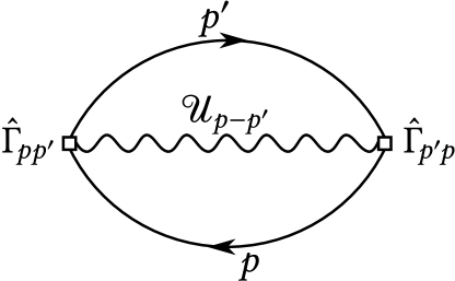
Figure 1: The first order diagram for the exchange energy of the electron gas. The momentum-dependent vertices $\hat{\Gamma}_{\bm{p}\bm{p}^{\prime}}$ of Eq. (6) reflect the PSOI contribution to the energy.

We treat the e-e interaction of Eq. (7) in a Hartree-Fock (HF) approximation. The Hartree (direct) contribution is not modified by the PSOI. Indeed, for the Hartree part of Eq. (7) $\bm{p}_{1}=\bm{p}_{2}$ and $\bm{p}_{1}^{\prime}=\bm{p}_{2}^{\prime}$, nullifying the SOI parts of interaction vertexes, $\hat{\Gamma}$, Eq. (6), due to the vector products of identical momenta. As a result, the Hartree term is compensated by the positive charge of the lattice and is absent in charge neutral systems. The Fock (exchange) contribution comes from the “oyster” diagram of Fig. 1. It is given by

$$E_{\mathrm{xc}}=-\frac{1}{2}\sum_{\bm{p}\bm{p}^{\prime}}\mathcal{U}_{\bm{p}-\bm{p}^{\prime}}\operatorname{Tr}\{\hat{G}_{\bm{p}}\hat{\Gamma}_{\bm{p}\bm{p}^{\prime}}\hat{G}_{\bm{p}^{\prime}}\hat{\Gamma}_{\bm{p}^{\prime}\bm{p}}\}\,,$$ (39)

where $\hat{G}_{\bm{p}}$ is the equal-time electron Green function.

To reach a spin-polarized state, one may assume a symmetry-breaking in any given direction, say along the $z$-axis. Under this assumption, the Green function takes the form 

$$\hat{G}_{\bm{p}}=\mathcal{G}_{0}(\bm{p})\hat{\sigma}_{0}+\mathcal{G}_{3}(\bm{p})\hat{\sigma}_{3}\;,$$ (40)

or explicitly,

$$\hat{G}_{\bm{p}}=\begin{pmatrix}n_{+}(\bm{p})&0\\ 0&n_{-}(\bm{p})\end{pmatrix}\,,$$ (41)

where $n_{\pm}(\bm{p})$ are occupation numbers of a state $\bm{p}$ by electrons with the two spin projections. Computing the trace in Eq. (39) one obtains

$$\begin{split}E_{\mathrm{xc}}=&{}-\sum_{\bm{p}\bm{p}^{\prime}}e^{2}\mathcal{U}_{\bm{p}-\bm{p}^{\prime}}\left\{\mathcal{G}_{0}(\bm{p})\mathcal{G}_{0}(\bm{p}^{\prime})+\mathcal{G}_{3}(\bm{p})\mathcal{G}_{3}(\bm{p}^{\prime})\right\}\\ &{}-\sum_{\bm{p}\bm{p}^{\prime}}\alpha_{pp^{\prime}}^{2}\mathcal{U}_{\bm{p}-\bm{p}^{\prime}}\left\{\mathcal{G}_{0}(\bm{p})\mathcal{G}_{0}(\bm{p}^{\prime})(\bm{\mathcal{M}}\cdot\bm{\mathcal{M}})+\mathcal{G}_{3}(\bm{p})\mathcal{G}_{3}(\bm{p}^{\prime})(\mathcal{M}_{z}^{2}-\mathcal{M}_{x}^{2}-\mathcal{M}_{y}^{2})\right\}\,,\end{split}$$ (42)

with $\bm{\mathcal{M}}\equiv\bm{\mathcal{M}}(\bm{p},\bm{p}^{\prime})=[\bm{p}\times\bm{p}^{\prime}]$. The first line of this equation is a common exchange energy of the Coulomb-interacting electron gas [64]. The second line is the PSOI contribution to the exchange energy. Notice that, unlike the Cooper channel above, the linear in $\alpha$ term is absent.

IV.2 Paramagnetic phase

In the paramagnetic electron state $n_{-}(\bm{p})=n_{+}(\bm{p})\equiv n(\bm{p})$ and Eq. (42) takes the form

$$\begin{split}E_{\mathrm{xc}}=&{}-\sum_{\bm{p}\bm{p}^{\prime}}e^{2}\mathcal{U}_{\bm{p}-\bm{p}^{\prime}}n(\bm{p})n(\bm{p}^{\prime})\\ &{}-\sum_{\bm{p}\bm{p}^{\prime}}\alpha_{pp^{\prime}}^{2}\mathcal{U}_{\bm{p}-\bm{p}^{\prime}}n(\bm{p})n(\bm{p}^{\prime})\bm{\mathcal{M}}^{2}(\bm{p},\bm{p}^{\prime})\,.\end{split}$$ (43)

Taking variation with respect to $n(\bm{p})$, one finds the HF effective dispersion of the form

$$\begin{split}V_{\bm{p}}^{\mathrm{HF}}={}&\frac{p^{2}}{2m}-2\sum_{\bm{p}^{\prime}}e^{2}\mathcal{U}_{\bm{p}-\bm{p}^{\prime}}n(\bm{p}^{\prime})\\ &{}-2\sum_{\bm{p}^{\prime}}\alpha_{pp^{\prime}}^{2}\mathcal{U}_{\bm{p}-\bm{p}^{\prime}}n(\bm{p}^{\prime})\bm{\mathcal{M}}^{2}(\bm{p},\bm{p}^{\prime})\,.\end{split}$$ (44)

In what follows, we assume a short-ranged, momentum-independent e-e interaction potential, $\mathcal{U}_{\bm{p}-\bm{p}^{\prime}}\equiv\mathcal{U}_{0}$, and adopt a specific momentum dependence for the SOI magnitude, 

$$\alpha_{pp^{\prime}}^{2}=\alpha^{2}\frac{\Lambda^{2}}{(\Lambda+p^{2})(\Lambda+{p^{\prime}}^{2})}\,,$$ (45)

where $\Lambda/2m$ is an energy scale of the order of the band gap. This is a simplest functional form that captures the decreasing magnitude of SOI as momentum increases. We stress that by neglecting the momentum dependence of $\alpha$ one could infer that the interaction parameter of the PSOI increases indefinitely as the electron concentration grows [35]. However, an extremely dense electron gas should essentially behave as non-interacting. To avoid the contradiction, the theory of the PSOI must be generalized to account for the momentum dependence of the SOI magnitude.

The ground state is constructed by filling the quantum states of the lowest energy. These states have the least momentum when the HF potential $V_{\bm{p}}^{\mathrm{HF}}$ increases monotonically with $p$. However, this is not the case with the potential of Eq. (44). The momentum dependence of $\bm{\mathcal{M}}(\bm{p},\bm{p}^{\prime})$ makes the effective dispersion non-monotonous, creating a moat-like dispersion. Consequently, it becomes beneficial for electrons to populate states with higher momentum — a distinct feature of the PSOI. This fact eventually leads to the topological Lifshitz transition.

To see this, first assume that electrons in a 3D gas with concentration $n$ form a Fermi sea enclosed by a spherical Fermi surface of radius $k_{F}={(3\pi^{2}n)}^{1/3}$, with $n(\bm{p})=\theta(k_{F}-\lvert\bm{p}\rvert)$. Such distribution function generates a spherically symmetric effective dispersion of the form

$$V_{\bm{p}}^{\mathrm{HF}}=\frac{p^{2}}{2m}-e^{2}\mathcal{U}_{0}n-\frac{2\alpha^{2}}{3\pi^{2}}\mathcal{U}_{0}\frac{\Lambda^{2}p^{2}}{\Lambda+p^{2}}\,\Xi(k_{F})\,.$$ (46)

The factor $\Xi(k_{F})$ is given by

$$\Xi(k_{F})=\frac{k_{F}^{3}}{3}-k_{F}\Lambda+\Lambda^{\frac{3}{2}}\arctan\frac{k_{F}}{\sqrt{\Lambda}}\,,$$ (47)

and interpolates between $\Xi(k_{F})\approx k_{F}^{5}/5\Lambda$ for $k_{F}\ll\sqrt{\Lambda}$ and $\Xi(k_{F})\approx k_{F}^{3}/3$ for $k_{F}\gg\sqrt{\Lambda}$.

Figure 2: The effective dispersion $V_{\bm{p}}^{\mathrm{HF}}$ as a function of momentum for two values of the SOI magnitude. The position of the Fermi momentum is shown by a vertical dotted line. The occupied states are shown in color. The Fermi surface is a sphere, as shown in the inset.

The effective mass of the electron diverges when the SOI magnitude $\alpha$ equals to

$$\alpha_{0}=\sqrt{\frac{3\pi^{2}}{4m\mathcal{U}_{0}\Lambda\Xi(k_{F})}}\,,$$ (48)

with a flat band forming around the Brillouin zone center. The dependence of the effective dispersion on the momentum becomes non-monotonous as soon as $\alpha>\alpha_{0}$, see Fig. 2. A minimum appears for a finite momentum, which depends on $\alpha$. For a given electron concentration, there exist a critical $\alpha_{1}$ such that for $\alpha\leq\alpha_{1}$ all states with $\lvert\bm{p}\rvert\leq k_{F}$ are occupied. This renders the Fermi surface as a sphere, in agreement with our initial assumption.

The critical value of $\alpha_{1}$ is inferred from

$$V_{\bm{p}}^{\mathrm{HF}}\big{|}_{p=0}=V_{\bm{p}}^{\mathrm{HF}}\big{|}_{p=k_{F}}$$ (49)

to give $\alpha_{1}=\alpha_{0}\sqrt{1+k_{F}^{2}/\Lambda}$. For $\alpha>\alpha_{1}$ states with the lowest energy no longer correspond to the smallest momenta. Instead, they are found in a range of momenta $k_{F_{1}}\leq\lvert\bm{p}\rvert\leq k_{F_{2}}$, forming a hollow spherical shell. This behavior is illustrated in Fig. 3. Such a transformation signals a Lifshitz transition, changing a topology of the Fermi surface.

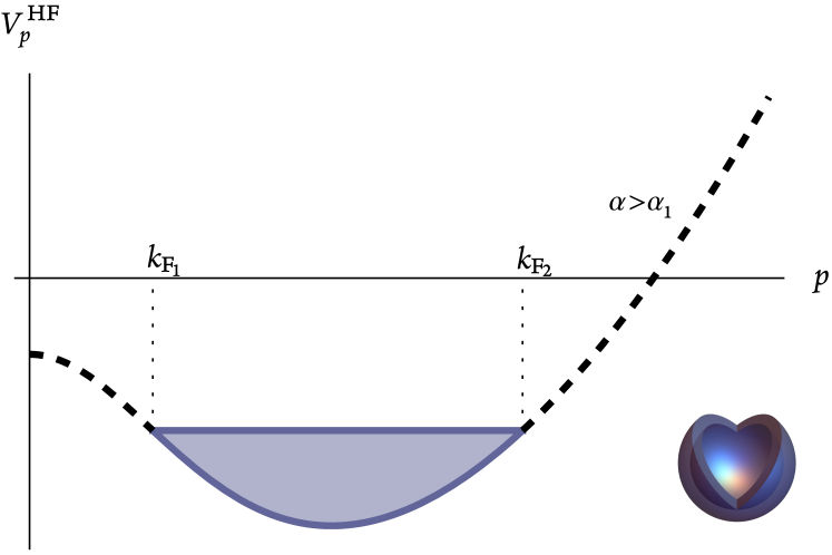
Figure 3: The effective dispersion $V_{\bm{p}}^{\mathrm{HF}}$ as a function of momentum for the larger-than-critical value of the SOI magnitude. The populated states are enclosed by a shell-like Fermi surface.

The corresponding distribution function takes the form

$$n(\bm{p})=\theta(\lvert\bm{p}\rvert-k_{F_{1}})\theta(k_{F_{2}}-\lvert\bm{p}\rvert)\,,$$ (50)

where the two Fermi momenta are related by a requirement of the fixed electron concentration, $k_{F_{2}}^{3}-k_{F_{1}}^{3}=3\pi^{2}n$. Such a distribution gives rise to a self-consistent solution provided that

$$V_{\bm{p}}^{\mathrm{HF}}\big{|}_{p=k_{F_{1}}}=V_{\bm{p}}^{\mathrm{HF}}\big{|}_{p=k_{F_{2}}}\,.$$ (51)

The effective dispersion calculated with the distribution function (50) is

$$V_{\bm{p}}^{\mathrm{HF}}=\frac{p^{2}}{2m}-e^{2}\mathcal{U}_{0}n-\frac{2\alpha^{2}\mathcal{U}_{0}}{3\pi^{2}}\frac{\Lambda^{2}p^{2}}{\Lambda+p^{2}}\left[\Xi(k_{F_{2}})-\Xi(k_{F_{1}})\right]\,.$$ (52)

Equations (51)-(52) lead to the following relation that allows one to find the two Fermi momenta,

$$\alpha^{2}[\Xi(k_{F_{2}})-\Xi(k_{F_{1}})]=\left(1+\frac{k_{F_{1}}^{2}}{\Lambda}\right)\left(1+\frac{k_{F_{2}}^{2}}{\Lambda}\right)\frac{3\pi^{2}}{4m\mathcal{U}_{0}\Lambda}\,.$$ (53)

As soon as $\alpha>\alpha_{1}$, the solution of this equation emerges with $k_{F_{1}}>0$, which determines the position of the shell boundaries in the momentum space.

The total energy per one electron, calculated self-consistently from Eq. (43) and taking into account the kinetic energy of the electrons filling the shell in the momentum space, equals

$$\begin{split}\varepsilon=&{}\frac{1}{10\pi^{2}n}\frac{k_{F_{2}}^{5}-k_{F_{1}}^{5}}{m}-e^{2}\mathcal{U}_{0}\frac{n}{4}\\ &{}-\frac{\alpha^{2}}{6\pi^{4}n}\mathcal{U}_{0}\Lambda^{2}{\left[\Xi(k_{F_{2}})-\Xi(k_{F_{1}})\right]}^{2}\,.\end{split}$$ (54)

This expression is valid for both shell-like ($\alpha>\alpha_{1}$) and spherical ($\alpha\leq\alpha_{1}$) Fermi surfaces, with $k_{F_{1}}=0$ in the latter case.

IV.3 Ferromagnetic phase

In a fully spin-polarized case of $n_{-}(\bm{p})=0$, the Eq. (42) reduces to

$$\begin{split}E_{\mathrm{xc}}=&{}-\frac{1}{2}\sum_{\bm{p}\bm{p}^{\prime}}e^{2}\mathcal{U}_{\bm{p}-\bm{p}^{\prime}}n(\bm{p})n(\bm{p}^{\prime})\\ &{}-\frac{1}{2}\sum_{\bm{p}\bm{p}^{\prime}}\alpha_{pp^{\prime}}^{2}\mathcal{U}_{\bm{p}-\bm{p}^{\prime}}n(\bm{p})n(\bm{p}^{\prime})\mathcal{M}_{z}^{2}(\bm{p},\bm{p}^{\prime})\,,\end{split}$$ (55)

with the corresponding HF dispersion given by

$$\begin{split}V_{\bm{p}}^{\mathrm{HF}}={}&\frac{p^{2}}{2m}-\sum_{\bm{p}^{\prime}}e^{2}\mathcal{U}_{\bm{p}-\bm{p}^{\prime}}n(\bm{p}^{\prime})\\ &{}-\sum_{\bm{p}^{\prime}}\alpha_{pp^{\prime}}^{2}\mathcal{U}_{\bm{p}-\bm{p}^{\prime}}n(\bm{p}^{\prime})\mathcal{M}_{z}^{2}(\bm{p},\bm{p}^{\prime})\,.\end{split}$$ (56)

Assuming for a moment a fully spin-polarized spherical Fermi surface with

$$K_{F}=\sqrt[3]{2}k_{F}={(6\pi^{2}n)}^{\frac{1}{3}},$$ (57)

results in an anisotropic HF effective dispersion

$$V_{\bm{p}}^{\mathrm{HF}}=\frac{p^{2}}{2m}-e^{2}\mathcal{U}_{0}n-\frac{\alpha^{2}\mathcal{U}_{0}}{6\pi^{2}}\frac{\Lambda^{2}p^{2}_{\parallel}}{\Lambda+p^{2}}\,\Xi(K_{F})\,,$$ (58)

where $\bm{p}_{\parallel}\equiv(p_{x},p_{y},0)$ is the in-plane momentum. This indicates an increased in-plane effective mass and therefore an anisotropic pancake shape of the Fermi surface.

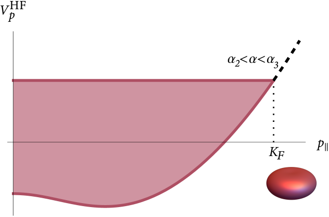
Figure 4: The effective dispersion $V_{\bm{p}}^{\mathrm{HF}}$ as a function of the in-plane momentum $p_{\parallel}$ at $p_{z}=0$ for weak SOI.

According to Eq. (58), surfaces of a constant energy may be parameterized by

$$(p^{2}+\Lambda)(p^{2}+\zeta)=4K^{2}p_{\parallel}^{2}\,,$$ (59)

with some constants $\zeta$ and $K$ to be determined self-consistently. For a small $\alpha$ the Fermi surface has a flattened ellipsoidal shape. However, upon the increase of $\alpha$ it undergoes a qualitative change. The in-plane effective mass diverges for the SOI magnitude of

$$\alpha_{2}=\sqrt{\frac{3\pi^{2}}{m\mathcal{U}_{0}\Lambda\Xi(K_{F})}}\,.$$ (60)

For $\alpha>\alpha_{3}$, where $\alpha_{3}=\alpha_{2}\sqrt{1+K_{F}^{2}/\Lambda}$, the Fermi surface acquires a toroidal shape, with the in-plane momenta limited to a range $K_{F_{1}}\leq p_{\parallel}\leq K_{F_{2}}$, while the normal momenta are concentrating near the center, $\lvert p_{z}\rvert<K_{F_{z}}$. As a result, the system undergoes the topological Lifshitz transition, with the Fermi surface genus changing from zero to one.

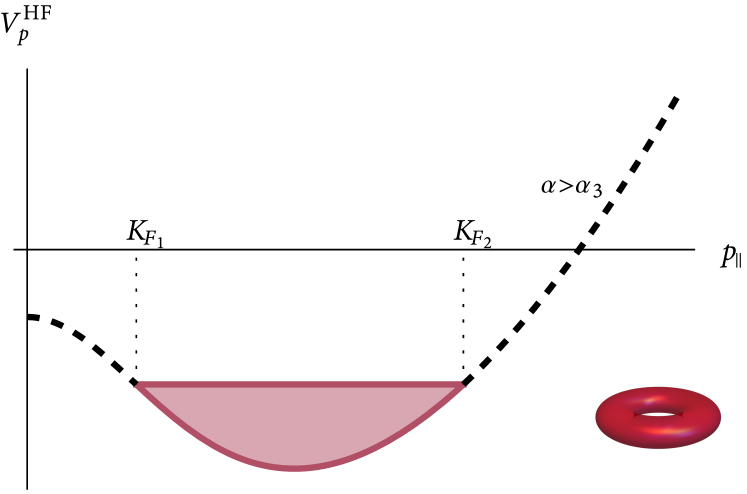
Figure 5: The effective dispersion $V_{\bm{p}}^{\mathrm{HF}}$ as a function of the in-plane momentum $p_{\parallel}$ at $p_{z}=0$, for the larger-than-critical value of the SOI magnitude. The Fermi surface is shaped like a torus.

One may show (see Appendix B) that the Fermi surface of Eq. (59) provides a self-consistent solution to Eq. (56). The total energy per one electron in the toroidal phase is equal to

$$\varepsilon=\frac{1}{4m}\left(4K^{2}-\Lambda-\zeta\right)-e^{2}\mathcal{U}_{0}\frac{n}{2}-\frac{\alpha^{2}\mathcal{U}_{0}\Lambda^{2}\Xi^{2}}{4n}\,,$$ (61)

with parameters $K$, $\zeta$ and $\Xi$ detailed in the Appenidix B. The results for the elliptical phase are quite similar; however, we have omitted them for brevity.

IV.4 Ferromagnetic Transitions

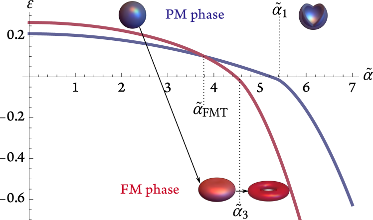
Figure 6: The energy per particle of a 3D electron gas, in units of $K_{F}^{2}/2m$, as a function of the dimensionless SOI magnitude $\tilde{\alpha}=\alpha K_{F}^{2}/e$, for $\tilde{\mathcal{U}}=1$ and $\Lambda/K_{F}^{2}=1$. The red curve corresponds to the ferromagnetic (FM) phase, and the blue curve to the paramagnetic (PM) one. The Stoner transition occurs at $\tilde{\alpha}=\tilde{\alpha}_{\mathrm{FMT}}$.

Figure 6 depicts the total HF energy per electron for both the paramagnetic and spin-polarized phases, plotted against the magnitude of the PSOI. This is represented for $\tilde{\mathcal{U}}=1$, where the e-e interaction parameter is normalized by the density of states as:

$$\tilde{\mathcal{U}}=e^{2}\mathcal{U}_{0}\frac{mK_{F}}{2\pi^{2}\hbar^{2}}\,.$$ (62)

At $\tilde{\alpha}=0$ the system is in the paramagnetic phase characterized by a spherical Fermi surface. As PSOI increases, the first order ferromagnetic transition occurs at a critical $\tilde{\alpha}=\tilde{\alpha}_{\mathrm{FMT}}$, which is accompanied by a Lifshitz transition to a state with an elliptical Fermi surface. In other words, both spin symmetry and the Fermi-surface symmetry simultaneously undergo a change at this point. As PSOI continues to increase, it induces a Lifshitz transition to a toroidal spin-polarized phase at $\tilde{\alpha}=\tilde{\alpha}_{3}$.

Figure 7: The energy per particle of a 3D electron gas as a function of the dimensionless SOI magnitude $\tilde{\alpha}=\alpha K_{F}^{2}/e$ for $\tilde{\mathcal{U}}=0.5$. The red curve corresponds to the ferromagnetic phase, and the blue curve to the paramagnetic one.

For a smaller interaction parameter of $\tilde{\mathcal{U}}=0.5$, the system can transition directly from the spherical paramagnetic phase to the toroidal spin-polarized phase, bypassing the elliptical phase, as depicted in Fig. 7. Conversely, with increased interaction, the system defaults to a ferromagnetic state at zero SOI due to the conventional Stoner instability. Yet, any non-zero value of $\alpha$ ensues breaking of the Fermi surface’s spherical symmetry. A further increase of $\alpha$ results into the Lifshitz transition from the ellipsoidal to the toroidal phase at $\tilde{\alpha}=\tilde{\alpha}_{3}$, as visualized in Fig. 8.

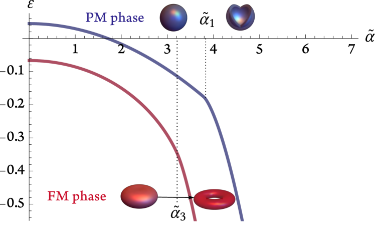
Figure 8: The energy per particle of a 3D electron gas as a function of the dimensionless SOI magnitude $\tilde{\alpha}=\alpha K_{F}^{2}/e$ for $\tilde{\mathcal{U}}=2$. The red curve corresponds to the ferromagnetic phase, and the blue curve to the paramagnetic one.

These findings are summarized in Fig. 9, showing the phase diagram in the coordinates of dimensionless SOI coupling $\tilde{\alpha}$ vs. the interaction strength $\tilde{\mathcal{U}}$. The paramagnet phase exhibits the first order transition to the fully polarized ferromagnet. The latter may come with either flat ellipsoidal or toroidal Fermi surfaces with the topological Lifshitz transition between them. The hollow spherical shell paramagnetic phase, discussed above, is not realized (at least within the present model), since the transition to the FM phase takes place before it becomes favorable. It is worth mentioning that the critical values of the parameters for the Stoner and Lifshitz transitions, obtained from the HF energy computations, are not expected to be quantitatively accurate. Correlation effects renormalize them, as indicated by the Monte Carlo simulations. Nevertheless, one may expect that the qualitative features of the phase diagram are still present, even with the account of the correlations.

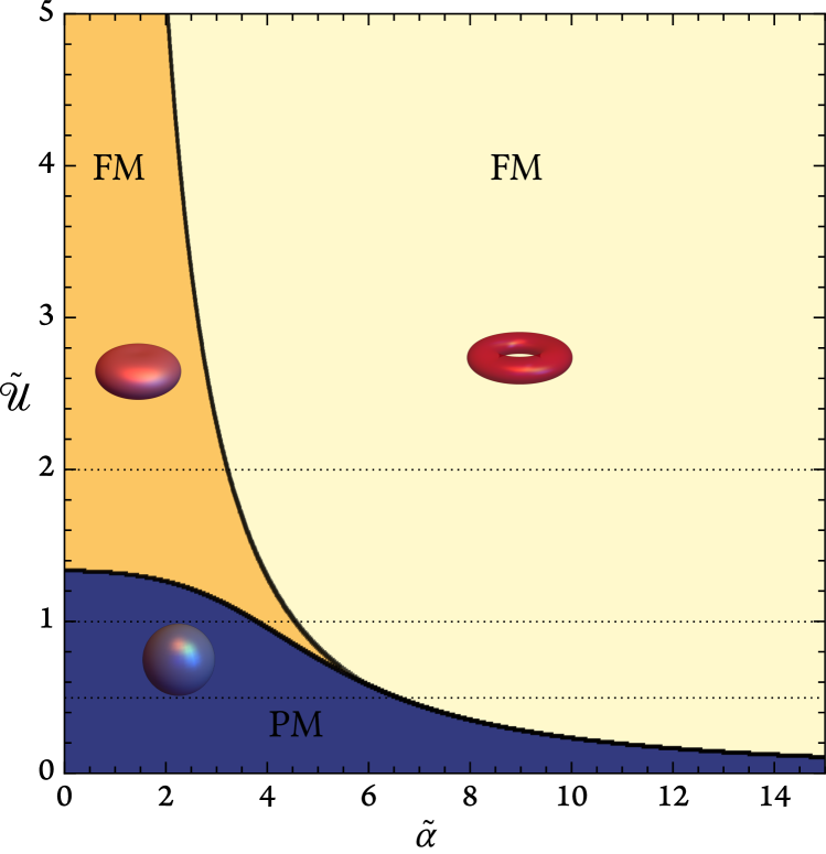
Figure 9: The phase diagram of the 3D Rashba system. Three horizontal cross-sections correspond to Figs. 6–8.

IV.5 Ferromagnetic Superconductors

Both ellipsoidal and toroidal fully polarized ferromagnets are susceptible to the development of the $p$-wave superconducting order, discussed in Section III. In this case only $\Delta^{+}_{\bm{p}}$ order parameter is realized, while $\Delta^{0}_{\bm{p}}$ and $\Delta^{-}_{\bm{p}}$ are absent (here $\pm,0$ stay for $m=\pm 1$ and $m=0$ projection of the Cooper pair spin angular momentum). Since the toroidal ferromagnetic phase requires a critical SOI strength, it is always formally within the parameter region with the superconducting ground state. In reality, if the disorder is sufficiently strong, the toroidal FM may not develop superconductivity down to zero temperature.

Consider the all spins up fully polarized state. Only the up-up component of the interaction matrix vertex $\hat{\Gamma}_{\bm{p}_{1}\bm{p}_{2}}$ remains, given by $\Gamma_{\bm{p}_{1}\bm{p}_{2}}^{+}=-e-i\alpha{[\bm{p}_{1}\times\bm{p}_{2}]}_{z}$. The corresponding BdG Hamiltonian is written in term of two-component spinors $\bar{\Psi}_{\bm{p}}=(\bar{\psi}_{\bm{p}\uparrow},\psi_{-\bm{p}\uparrow})$, and takes the form:

$$\hat{H}_{\mathrm{BdG}}=\sum_{\bm{p}}\,\bar{\Psi}_{\bm{p}}\begin{pmatrix}V^{\mathrm{HF}}_{\bm{p}}-\mu&\Delta^{+}_{\bm{p}}\\ \bar{\Delta}_{\bm{p}}^{+}&-V^{\mathrm{HF}}_{\bm{p}}+\mu\end{pmatrix}\Psi_{\bm{p}},$$ (63)

where the order parameter is odd: $\Delta_{-\bm{p}}^{+}=-\Delta_{\bm{p}}^{+}$. The corresponding self-consistency condition for the case of the short range interactions is

$$\Delta_{\bm{p}}^{+}=-2e\alpha\mathcal{U}_{0}\sum\limits_{\bm{p}_{2}}\,\frac{\tanh E_{\bm{p}_{2}}/2T}{2E_{\bm{p}_{2}}}\,\,\Delta_{\bm{p}_{2}}^{+}\,{[\bm{p}\times\bm{p}_{2}]}_{z}\,,$$ (64)

where $E_{\bm{p}}=\sqrt{(V^{\mathrm{HF}}_{\bm{p}}-\mu)^{2}+{\left\lvert\Delta_{\bm{p}}^{+}\right\rvert}^{2}}\,$. Since the HF effective dispersion, $V^{\mathrm{HF}}_{\bm{p}}$, is axially symmetric, i.e. independent on the azimuthal angle, $\phi_{\bm{p}}$, the self-consistency may be satisfied with the following ansatz:

$$\Delta_{\bm{p}}^{+}=\Delta\sin\theta_{\bm{p}}\,e^{-i\operatorname{sign}(\alpha)\phi_{\bm{p}}}=\frac{\Delta}{p}\,\big{(}p^{x}-i\operatorname{sign}(\alpha)p^{y}\big{)}\,.$$ (65)

This may be verified by performing $\phi_{\bm{p}_{2}}$ integration in Eq. (64). The amplitude $\Delta$ is then found from

$$1=e\lvert\alpha\rvert\mathcal{U}_{0}p_{F}^{2}\!\!\int\!\!\frac{p^{2}dp}{{(2\pi)}^{2}}\!\int_{0}^{\pi}\!\!\!d\theta\,\sin^{3}\!\theta\,\,\frac{\tanh E_{p,\theta}/2T}{E_{p,\theta}}\,,$$ (66)

Notice that the spin polarization restores the symmetry with respect $\alpha\to-\alpha$ even in 3D systems.

The coexisting FM and superconducting orders break rotational, time-reversal and global $U(1)$ symmetries. This puts the model into symmetry class D. The latter is not topological in 3D, though it does admit an integer Chern number in 2D. It is interesting to notice that the topological Lifshitz transition from elliptical to the toroidal Fermi surface has direct consequences for the superconducting order. Indeed, the $p$-wave superconductor with the order parameter $\Delta^{+}$ and the ellipsoidal Fermi surface is nodal with the two nodes on the flat parts of the ellipsoid (due to the $\sin\theta_{\bm{p}}$ factor in Eq. (65)). Once the Fermi surface transitions to the toroidal shape, the nodes disappear and the $p$-wave state $\Delta^{+}$ is fully gapped (similarly to its 2D counterpart). This may lead to a weak first order transition between the nodal and gapped groundstates, but its details require a further investigation.

IV.6 Manifestations of the ferromagnetic transitions

The FM state is, of course, associated with a net magnetic moment. This may be hard to detect due to, e.g., a domain structure (in presence of some uniaxial magnetic anisotropy). Moreover, the magnetic moment itself does not reveal the nature of the state and properties of its Fermi surface. Here we briefly discuss other observable manifestations of the FM transitions.

The first order transition between the isotropic PM state and an anisotropic FM state is associated with the jump in the electronic density of states at the Fermi surface. It may be detected thus through a measurement of the electronic specific heat. The onset of the anisotropy in the orbital space may lead to anisotropic behavior of transport coefficients. This issue requires a separate study, since its involves specific scattering mechanisms. The Lifshitz transition between the ellipsoidal and toroidal Fermi surfaces does not lead to a discontinuity in the density of states. It leads, however, to its nonanalitic behavior, $\nu(\tilde{\alpha})=\nu-\nu_{1}\sqrt{\tilde{\alpha}_{3}-\tilde{\alpha}}\,\theta(\tilde{\alpha}_{3}-\tilde{\alpha})$, on the ellipsoidal side of the transition. This may also lead to detectable features in the electronic specific heat.

Besides thermodynamic or transport measurements, one may detect Friedel oscillations of the electronic density, created by an impurity. Specifically, the emergence of the two Fermi momenta, $k_{F_{1}}$ and $k_{F_{2}}$, in the toroidal phase is reflected in a non-analytic behavior of a static charge susceptibility $\chi(q)$ at points $q=2k_{F_{1}}$, $q=2k_{F_{2}}$, and $q=k_{F_{1}}\pm k_{F_{2}}$. Consequently, the spatial profile of the Friedel oscillations contains the corresponding harmonics, which can be observed using STM. The reconstruction of the Fermi surface may be also visible in the periods of the Shubnikov-de Haas magnetoresistance oscillations [65]. Indeed, the oscillation periods are associated with the areas of extremal cross sections of the Fermi surface, which change abruptly at all FM transitions, considered above. Finally, the more delicate probes such as spin-resolved ARPES, polarized neutron scattering, or the state-of-the-art nano-SQUID magnetometers [66] can reveal information about the shape of the Fermi surface and a local magnetic moment.

V Concluding remarks

We discussed how Rashba spin-orbit coupling of conduction band electrons, a result of the band mixing with spin-orbit-split valence bands, manifests itself in electron-electron interactions effects. Projection of a multi-band model onto the conduction band degrees of freedom leads to a spin-dependent renormalization of the electron density, as seen in Eq. (3). Besides more familiar manifestations in the single-particle dispersion relation (for a broken inversion symmetry), RSOI modifies the electron-electron interaction vertex. This phenomenon, known as the pair SOI, emerges without the need for external electric fields or inversion symmetry breaking, relying instead on internal fluctuating electric fields of the Coulomb interactions between (renormalized) conduction band electrons.

We explored two consequences of PSOI. First, echoing the Kohn-Luttinger effect, PSOI induces $p$-wave superconducting pairing, driven purely by electron-electron interactions. This leads to distinct superconducting states in sufficiently clean materials. In 3D systems, the SOI constant $\alpha$ determines the nature of the superconducting order parameter, resulting in either nodal superconductivity along a spontaneously chosen direction or a node-less isotropic state. Strikingly, these phases mirror those in superfluid ³He, drawing an unexpected parallel between these systems.

In 2D systems, the $p$-wave state is fully gapped. It consists of two decoupled condensates of spin up and down electrons, polarized along the normal direction. The two condensate exhibit opposite Chern numbers. Their vortices (if spatially separated from each other) harbor Majorana states [67]. Stability of the latter depends if mutual interactions between vortices of the two condensates are repulsive (leading to stability) or attractive (leading to mutual anihilation).

The potential for carrying spin-polarized supercurrents in these superconductors is particularly intriguing. This could be achieved through spin injection from a ferromagnet or by imbalancing the condensates via external magnetic fields or proximity effects. The concept of a superconducting spin-valve, controllable by magnetic fields or ferromagnetic leads, emerges as an exciting application.

The second consequence of PSOI is its role in facilitating Stoner ferromagnetism, linked with the symmetry breaking in both spin and orbital spaces. This effect transforms the Fermi surface of the polarized itinerant electrons into ellipsoidal or toroidal shapes, leading to genus-changing topological Lifshitz transitions as a function of the SOI magnitude or interactions strength. The transition may have a number of observable manifestations in thermodynamic and transport properties, as well as in the spectra of Friedel and Shubnikov-de Haas oscillations. Finally, the anisotropic Stoner ferromagnet may coexist with the $p$-wave superconductor. If this is the case, the Lifshitz ellipsoidal to toroidal transition manifests itself as the transition between nodal and fully gapped superconducting states.

Appendix A Microscopic model of the RSOI

Here a microscopic derivation of the RSOI Hamiltonian is outlined, with a focus on a momentum dependence of the SOI coupling for a particularly simple case of a 2D electron system with the inversion symmetry. The approach is based on the symmetric Bernevig-Hughes-Zhang (BHZ) model [68]. This model is widely recognized for its capacity to describe various 2D systems with strong RSOI, across both topological and trivial phases.

The BHZ model is expressed in a four-band basis, denoted as $\mathcal{B}={\{\lvert\operatorname{E\!\uparrow}\rangle,\lvert\operatorname{H\!\uparrow}\rangle,\lvert\operatorname{E\!\downarrow}\rangle,\lvert\operatorname{H\!\downarrow}\rangle\}}^{\intercal}$. Within this basis, the states $\lvert\operatorname{E\!\uparrow}\rangle$ and $\lvert\operatorname{E\!\downarrow}\rangle$ consist of the electron- and light-hole band states, each carrying an angular momentum projection of $m_{J}=\pm 1/2$. Conversely, the states $\lvert\operatorname{H\!\uparrow}\rangle$ and $\lvert\operatorname{H\!\downarrow}\rangle$ correspond to the heavy-hole states, with an angular momentum projection of $m_{J}=\pm 3/2$. The Hamiltonian governing the envelope wave-function in this context is as follows

$$\hat{H}_{\mathrm{BHZ}}=\begin{bmatrix}m(\hat{p})&A\hat{p}_{+}&0&0\\ A\hat{p}_{-}&-m(\hat{p})&0&0\\ 0&0&m(\hat{p})&-A\hat{p}_{-}\\ 0&0&-A\hat{p}_{+}&-m(\hat{p})\end{bmatrix}\,.$$ (67)

Here

$$m(\hat{p})=m+B\hat{p}^{2}\,,$$ (68)

with $m$ the band gap, $B$ the bare dispersion curvature, and $A$ the band hybridization parameter. Then, $\hat{p}$ is the momentum operator, $\hat{p}_{\pm}=\hat{p}_{x}\pm i\hat{p}_{y}$.

The BHZ model inherently incorporates a strong SOI, premised on the assumption of an infinitely large spin-splitting in the valence band. Since the spin sectors are decoupled it is possible to treat them separately by considering a $2\times 2$ Hamiltonian

$$\hat{H}_{0}(\hat{p})=m(\hat{p})\tau_{3}+A(\hat{\bm{p}}\cdot\hat{\bm{\tau}})\,,$$ (69)

with $\hat{\tau}_{i}$ the pseudospin (subband) Pauli matrices. The Hamiltonian can be diagonalized

$$\hat{\mathcal{H}}_{0}(\hat{p})=\hat{U}(\hat{p})\hat{H}_{0}(\hat{p})\hat{U}^{+}(\hat{p})$$ (70)

by a unitary Foldy-Wouthuysen transformation

$$\hat{U}(\hat{p})=\cos\theta(\hat{p})+\sin\theta(\hat{p})\frac{(\hat{\bm{p}}\cdot\hat{\bm{\tau}})}{p}\tau_{3}$$ (71)

to acquire the form

$$\hat{\mathcal{H}}_{0}(\hat{p})=\varepsilon(\hat{p})\tau_{3}\,,$$ (72)

with the band dispersion

$$\varepsilon(\hat{p})=\sqrt{m^{2}(\hat{p})+A^{2}\hat{p}^{2}}\,,$$ (73)

and

$$\tan 2\theta(\hat{p})=-A\frac{\hat{p}}{m(\hat{p})}\,.$$ (74)

For a sufficiently small hybridization parameter the unitary operator (71) may be approximated as

$$\hat{U}(\hat{p})\approx 1-\frac{A}{2m(\hat{p})}(\hat{\bm{p}}\cdot\hat{\bm{\tau}})\tau_{3}-\frac{A^{2}\hat{p}^{2}}{8m^{2}(\hat{p})}+\mathcal{O}(A^{3})\,,$$ (75)

under the condition that $Ap\ll m(p)$.

In the context of the Dirac equation, this condition holds true only for limited momentum values near the minimum of the electron band. Within this regime, it gives rise to the conventional formula for the relativistic SOI, featuring a constant magnitude for $\alpha$, equal to $\alpha=e\lambdabar^{2}/4$, $\lambdabar$ being the Compton wavelength of the electron [69].

In contrast, the BHZ model presents a notable departure from this picture. By virtue of Eq. (68), the above expansion applies to both the small ($p\to 0$) and large ($p\gtrsim A/B$) values of momenta, provided $B\neq 0$. This broader applicability range allows for a generalized RSOI Hamiltonian capable of describing electron dynamics in the quantum states with large momenta.

Applying the unitary transformation to the Hamiltonian

$$\hat{H}(\hat{p})=\hat{H}_{0}(\hat{p})-e\varphi(\hat{\bm{r}}),$$ (76)

that describes the interaction with a scalar potential, one should take into account that the momentum-dependent operators $\hat{U}(\hat{p})$ do not commute with a position-dependent $\varphi(\hat{\bm{r}})$. The commutator terms generate the operator

$$\hat{\mathcal{V}}(\hat{p})=\frac{A}{2m(\hat{p})}\hat{\bm{\tau}}\cdot(-e\grad_{\bm{r}}\varphi\times\hat{\bm{p}})\frac{A}{2m(\hat{p})}\,.$$ (77)

Within the low-energy approximation one focuses on the electron dynamics in the conduction band by declaring the spinor components in the valence band to be small and keeping only the $\hat{\mathcal{V}}_{11}$ matrix element pertaining to the conduction band. Combining the terms $\hat{\mathcal{V}}_{11}^{(s)}$ from both spin sectors the following generalized RSOI Hamiltonian in the reduced conduction band basis is obtained,

$$\hat{H}_{\mathrm{RSOI}}(\hat{p})=\frac{A}{2m(\hat{p})}\hat{\bm{\sigma}}\cdot(-e\grad_{\bm{r}}\varphi\times\hat{\bm{p}})\frac{A}{2m(\hat{p})}\,,$$ (78)

with $\hat{\bm{\sigma}}$ the real spin Pauli vector. Equation (78) is consistent with earlier result of Ref. [70] in the limit of small momenta. This gives rise to the interaction vertex of Eq. (6) with a momentum-dependent SO coupling of the form

$$\alpha_{p_{1}p_{2}}=\frac{A^{2}}{4m(p_{1})m(p_{2})}\,,$$ (79)

which incorporates the decrease of SOI magnitude at large momenta.

Appendix B Self-consistent HF solution

Here, the toroidal Fermi surface is demonstrated to be a self-consistent solution of Eq. (56). The derivation proceeds in two steps. First, the effective dispersion in Eq. (56) is found assuming that the electrons occupy the toric region in the momentum space limited by the Fermi surface of Eq. (59). Second, the isoenergetic surface of the resulting HF potential is verified to be that of Eq. (59) under the proper choice of parameters, which results in self-consistency conditions.

A change of variables $q_{\parallel}^{2}=p^{\prime 2}_{\parallel}+\delta^{2}$, $q_{z}=p^{\prime}_{z}$ with $\delta=(\Lambda-\zeta)/4K$ transforms Eq. (59) to the canonical equation of a torus,

$${(q^{2}+K^{2}-k^{2})}^{2}=4K^{2}q_{\parallel}^{2}\,,$$ (80)

where

$$k^{2}={(K-\delta)}^{2}-\zeta\,.$$ (81)

The torus interior, $\mathcal{D}$, can be parametrized by

$$\begin{split}q_{x}&=(K+\eta\cos\theta)\cos\phi\,,\\ q_{y}&=(K+\eta\cos\theta)\sin\phi\,,\\ q_{z}&=\eta\sin\theta\,,\\ \end{split}$$ (82)

with $\eta\in(0,k)$, $\phi\in(0,2\pi)$, and $\theta\in(0,2\pi)$. The Jacobian of the transformation is $J(\eta,\theta)=\eta(K+\eta\cos\theta)$.

The momentum-dependent factor that enters Eq. (56) is

$$\mathcal{M}_{z}^{2}(\bm{p},\bm{p}^{\prime})={[\bm{p}\times\bm{p^{\prime}}]}^{2}_{z}=p^{2}_{\parallel}p^{\prime 2}_{\parallel}\sin^{2}\widehat{\bm{p}_{\parallel}\bm{p}^{\prime}_{\parallel}}\,.$$ (83)

Due to the axial symmetry of the problem, the $\sin^{2}\widehat{\bm{p}_{\parallel}\bm{p}^{\prime}_{\parallel}}$ averages to $1/2$ when integrated over the polar angle. The PSOI contribution to the HF potential of Eq. (56) takes the form

$$\begin{split}V_{\mathrm{PSOI}}(\bm{p})=&{}-\frac{\alpha^{2}\mathcal{U}_{0}\Lambda^{2}}{\Lambda+p^{2}}\int\frac{d^{3}p^{\prime}}{{(2\pi)}^{3}}\frac{{[\bm{p}\times\bm{p^{\prime}}]}^{2}_{z}}{\Lambda+p^{\prime 2}}\\ =&{}-\frac{\alpha^{2}\mathcal{U}_{0}\Lambda^{2}p_{\parallel}^{2}}{\Lambda+p^{2}}\frac{\Xi}{2}\,,\end{split}$$ (84)

where

$$\begin{split}\Xi=&{}\int\frac{d^{3}p^{\prime}}{{(2\pi)}^{3}}\frac{p^{\prime 2}_{\parallel}}{\Lambda+p^{\prime 2}}=\int_{\mathcal{D}}\frac{d\eta d\theta d\phi}{{(2\pi)}^{3}}J(\eta,\theta)\frac{{(K+\eta\cos\theta)}^{2}-\delta^{2}}{\eta^{2}+2K\eta\cos\theta+K^{2}+\Lambda-\delta^{2}}\\ ={}&\frac{1}{96\pi K^{3}}\Big{[}k^{6}-k^{4}\left(3\delta^{2}+\varkappa+3K^{2}-3\Lambda\right)+k^{2}\left(\left(\delta^{2}-\Lambda\right)\left(3\delta^{2}+2\varkappa-3\Lambda\right)+21K^{4}+2K^{2}(\varkappa-6\Lambda)\right)\\ &{}+\left({\left(\delta^{2}-\Lambda\right)}^{2}+K^{4}-2K^{2}\left(\delta^{2}+5\Lambda\right)\right)\left(-\delta^{2}-\varkappa+K^{2}+\Lambda\right)\Big{]}\,,\end{split}$$ (85)

with

$$\varkappa\equiv\sqrt{\left[{(K+k)}^{2}+\Lambda-\delta^{2}\right]\left[{(K-k)}^{2}+\Lambda-\delta^{2}\right]}\,.$$ (86)

Consequently, the total HF potential of Eq. (56) acquires the form

$$V_{\bm{p}}^{\mathrm{HF}}=\frac{p^{2}}{2m}-e^{2}\mathcal{U}_{0}n-\frac{\alpha^{2}\mathcal{U}_{0}\Lambda^{2}p_{\parallel}^{2}}{\Lambda+p^{2}}\frac{\Xi}{2}\,.$$ (87)

The Fermi surface of $V_{\bm{p}}^{\mathrm{HF}}=E_{F}$ for the electron dispersion of Eq. (87) has indeed the assumed form of Eq. (59), provided that the following self-consistency conditions hold:

$$K^{2} =\frac{m\alpha^{2}\mathcal{U}_{0}\Lambda^{2}}{4}\Xi\,,$$ (88)

$$\zeta =-2m(E_{F}+e^{2}\mathcal{U}_{0}n)\,,$$ (89)

which should be supplemented by Eq. (81) and the relation $k^{2}K=4\pi n$ between the Fermi sea volume and electron concentration. The system of these four equations allows one to find the three quantities: $K$, $k$, and $\zeta$, which determine the geometry of the Fermi surface, as well as the Fermi energy $E_{F}$.

Appendix C 2D Rashba Ferromagnets

Here the effects of PSOI are explored in 2D electron systems. To begin, consider a particular case of a system symmetric with respect to the inversion of the normal $z\to-z$. Within this framework, the PSOI emerges solely due to the in-plane Coulomb fields, created by interacting electrons. The symmetric 2D structures represent a fascinating object of research in their own right, as they are realized through freely suspended 2D layers, with a focus on amplifying the effects of e-e interactions [71].

The expressions for the effective electron dispersion and exchange energy presented in Section IV also apply here, with the integration running over the 2D momentum space. The analysis is performed within the BHZ model [68], with the specific form of the spin-orbit coupling as given by Eq. (79), and kinetic energy of Eq. (73).

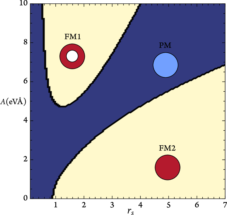
Figure 10: The phase diagram for the spin polarization of a 2D electron gas with PSOI. The system parameters are those typically found in 2D Rashba materials [2]: $m=$0.01\text{\,}\mathrm{e}\mathrm{V}$$, $B=$50\text{\,}{\mathrm{\text{\r{A}}}^{2}}\mathrm{e}\mathrm{V}$$, $d=$50\text{\,}\mathrm{\text{\r{A}}}$$, $\epsilon=20$.

The interaction in 2D layers of Rashba materials is governed by the Rytova-Keldysh potential [72, 73]

$$\mathcal{U}_{\bm{q}}=\frac{2\pi}{q(1+ql)}\,,$$ (90)

where the length $l$ is a phenomenological parameter of the theory, which generally speaking should be determined from the first-principles calculations [74]. It can be estimated from the layer polarizability as $l=\epsilon d/2$, where $d$ stands for the layer thickness, and $\epsilon$ is the in-plane component of the dielectric tensor of the corresponding bulk material.

Spin polarization is controlled by the balance between the kinetic and exchange interaction (both Coulomb and PSOI) energies. The degree of the spin polarization is found by identifying the minimum of the total HF energy. As the three contributions display distinct density dependencies [35], it is anticipated that the lowest energy state will be FM in two regions: at a low density as a result of Coulomb exchange and at a high density due to PSOI.

These expectations are confirmed by Fig. 10, which presents the phase diagram of system magnetization vs. BHZ velocity $A$, which serves as the magnitude of the PSOI, and $r_{s}$ values .

One identifies two distinct, fully spin-polarized phases. A new region of the FM phase emerges at lower $r_{s}$ values when the PSOI magnitude surpasses a certain critical threshold. Its Fermi surface exhibits a shape of annulus $k_{F_{1}}\leq k\leq k_{F_{2}}$, which can be viewed as a 2D projection of the toroidal Fermi-surface discussed in Section IV.3.

This result is seemingly at odds with the conventional perspective on Stoner ferromagnetism, which is expected to only occur at sufficiently low electron densities. Such transition, driven by the Coulomb exchange, is indeed present as FM2 phase in Fig. 10 in a FM region of high $r_{s}$. It exhibits a circular Fermi surface. Conversely, the annular FM1 phase emerges in the regime of a dense electron gas, where the PSOI interactions are strong due to their strong momentum dependence. Both FM phases exhibit spin polarization normal to the plane, with the easy axis set by the PSOI. This is also different from the conventional 2D Stoner ferromagnetism, where the spin rotation symmetry can spontaneously break in any direction.

The emergence of the annular FM phase is due to the moat-band dispersion created by PSOI. Notice that the single-particle Rashba effect, due to a normal electric field $\mathcal{E}_{z}$, also leads to a similar moat-band. In the latter scenario, the electron system displays a momentum-locked chiral spin texture. In the annular FM phase, on the other hand, electrons exhibit complete spin polarization in the $z$-direction.

In both FM1 and FM2 phases, electrons remain unaffected by the single-particle RSOI, $H_{\mathrm{RSOI}}=\alpha(\bm{\sigma}\times\bm{\mathcal{E}}_{z})\cdot\bm{p}$, since the magnetization, $\bm{\sigma}$, is colinear with the external field. Only when the electric field surpasses a certain critical magnitude of the order of $\mathcal{E}_{c}\simeq v_{F}/\alpha$, the $z$-polarized FM phases lose their stability. A transition to an alternative spin-polarized phase, potentially exhibiting nematic order, is plausible [75, 76, 77] at a larger external field.

References

- Bihlmayer et al. [2022] G. Bihlmayer, P. Noël, D. V. Vyalikh, E. V. Chulkov, and A. Manchon, Rashba-like physics in condensed matter, Nature Reviews Physics 10.1038/s42254-022-00490-y (2022).
- Manchon et al. [2015] A. Manchon, H. C. Koo, J. Nitta, S. M. Frolov, and R. A. Duine, New perspectives for Rashba spin-orbit coupling, Nature materials 14, 871 (2015).
- Bihlmayer et al. [2015] G. Bihlmayer, O. Rader, and R. Winkler, Focus on the Rashba effect, New Journal of Physics 17, 050202 (2015).
- Dyakonov [2017] M. I. Dyakonov, ed., Spin Physics in Semiconductors, Springer Series in Solid-State Sciences, Vol. 157 (Springer International Publishing, 2017).
- Glazov [2018] M. M. Glazov, Electron & nuclear spin dynamics in semiconductor nanostructures, Series on Semiconductor Science and Technology, Vol. 23 (Oxford University Press, 2018).
- Dieny et al. [2020] B. Dieny, I. L. Prejbeanu, K. Garello, P. Gambardella, P. Freitas, R. Lehndorff, W. Raberg, U. Ebels, S. O. Demokritov, J. Akerman, A. Deac, P. Pirro, C. Adelmann, A. Anane, A. V. Chumak, A. Hirohata, S. Mangin, S. O. Valenzuela, M. C. Onbaşlı, M. d’Aquino, G. Prenat, G. Finocchio, L. Lopez-Diaz, R. Chantrell, O. Chubykalo-Fesenko, and P. Bortolotti, Opportunities and challenges for spintronics in the microelectronics industry, Nature Electronics 3, 446 (2020).
- He et al. [2022] Q. L. He, T. L. Hughes, N. P. Armitage, Y. Tokura, and K. L. Wang, Topological spintronics and magnetoelectronics, Nature Materials 21, 15 (2022).
- Kim et al. [2022] S. K. Kim, G. S. D. Beach, K.-J. Lee, T. Ono, T. Rasing, and H. Yang, Ferrimagnetic spintronics, Nature Materials 21, 24 (2022).
- King et al. [2011] P. D. C. King, R. C. Hatch, M. Bianchi, R. Ovsyannikov, C. Lupulescu, G. Landolt, B. Slomski, J. H. Dil, D. Guan, J. L. Mi, E. D. L. Rienks, J. Fink, A. Lindblad, S. Svensson, S. Bao, G. Balakrishnan, B. B. Iversen, J. Osterwalder, W. Eberhardt, F. Baumberger, and P. Hofmann, Large tunable Rashba spin splitting of a two-dimensional electron gas in , Phys. Rev. Lett. 107, 096802 (2011).
- Ishizaka et al. [2011] K. Ishizaka, M. Bahramy, H. Murakawa, M. Sakano, T. Shimojima, T. Sonobe, K. Koizumi, S. Shin, H. Miyahara, A. Kimura, et al., Giant Rashba-type spin splitting in bulk BiTeI, Nature materials 10, 521 (2011).
- Singh and Romero [2017] S. Singh and A. H. Romero, Giant tunable Rashba spin splitting in a two-dimensional BiSb monolayer and in BiSb/AlN heterostructures, Phys. Rev. B 95, 165444 (2017).
- Manzeli et al. [2017] S. Manzeli, D. Ovchinnikov, D. Pasquier, O. V. Yazyev, and A. Kis, 2D transition metal dichalcogenides, Nature Reviews Materials 2, 17033 (2017).
- Varignon et al. [2018] J. Varignon, L. Vila, A. Barthelemy, and M. Bibes, A new spin for oxide interfaces, Nature Physics 14, 322 (2018).
- Otrokov et al. [2018] M. M. Otrokov, I. I. Klimovskikh, F. Calleja, A. M. Shikin, O. Vilkov, A. G. Rybkin, D. Estyunin, S. Muff, J. H. Dil, A. V. de Parga, et al., Evidence of large spin-orbit coupling effects in quasi-free-standing graphene on Pb/Ir (111), 2D Materials 5, 035029 (2018).
- López et al. [2019] A. López, L. Colmenárez, M. Peralta, F. Mireles, and E. Medina, Proximity-induced spin-orbit effects in graphene on Au, Phys. Rev. B 99, 085411 (2019).
- Niesner et al. [2016] D. Niesner, M. Wilhelm, I. Levchuk, A. Osvet, S. Shrestha, M. Batentschuk, C. Brabec, and T. Fauster, Giant Rashba splitting in organic-inorganic perovskite, Phys. Rev. Lett. 117, 126401 (2016).
- Briggeman et al. [2020] M. Briggeman, J. Li, M. Huang, H. Lee, J.-W. Lee, K. Eom, C.-B. Eom, P. Irvin, and J. Levy, Engineered spin-orbit interactions in -based 1D serpentine electron waveguides, Science Advances 6, eaba6337 (2020), https://www.science.org/doi/pdf/10.1126/sciadv.aba6337 .
- Briggeman et al. [2021] M. Briggeman, H. Lee, J.-W. Lee, K. Eom, F. Damanet, E. Mansfield, J. Li, M. Huang, A. J. Daley, C.-B. Eom, P. Irvin, and J. Levy, One-dimensional Kronig-Penney superlattices at the interface, Nature Physics 17, 782 (2021).
- Mikheev et al. [2023] E. Mikheev, I. T. Rosen, J. Kombe, F. Damanet, M. A. Kastner, and D. Goldhaber-Gordon, A clean ballistic quantum point contact in strontium titanate, Nat. Electron. 6, 417 (2023).
- Beyl et al. [2015] S. Beyl, P. P. Orth, M. Scheurer, and J. Schmalian, Superconducting fluctuations in systems with Rashba-spin-orbit coupling, Verhandlungen der Deutschen Physikalischen Gesellschaft (2015).
- Wang et al. [2015] Z. Wang, D.-K. Ki, H. Chen, H. Berger, A. H. MacDonald, and A. F. Morpurgo, Strong interface-induced spin–orbit interaction in graphene on , Nature Communications 6, 8339 (2015).
- Sun et al. [2023] L. Sun, L. Rademaker, D. Mauro, A. Scarfato, Á. Pásztor, I. Gutiérrez-Lezama, Z. Wang, J. Martinez-Castro, A. F. Morpurgo, and C. Renner, Determining spin-orbit coupling in graphene by quasiparticle interference imaging, Nature Communications 14, 10.1038/s41467-023-39453-x (2023).
- Zollner et al. [2023] K. Zollner, S. M. João, B. K. Nikolić, and J. Fabian, Twist- and gate-tunable proximity spin-orbit coupling, spin relaxation anisotropy, and charge-to-spin conversion in heterostructures of graphene and transition-metal dichalcogenides (2023), arXiv:2310.17907 [cond-mat.mes-hall] .
- Bychkov and Rashba [1984] Y. A. Bychkov and E. I. Rashba, Properties of a 2D electron gas with lifted spectral degeneracy, JETP Lett 39, 78 (1984).
- Engel et al. [2007] H.-A. Engel, E. I. Rashba, and B. I. Halperin, Theory of spin Hall effects in semiconductors, in Handbook of Magnetism and Advanced Magnetic Materials (John Wiley & Sons, Ltd, 2007).
- Winkler [2003] R. Winkler, Spin-orbit Coupling Effects in Two-Dimensional Electron and Hole Systems, edited by J. Kühn, T. Müller, A. Ruckenstein, F. Steiner, J. Trümper, and P. Wölfle, Springer Tracts in Modern Physics, Vol. 191 (Springer, Berlin/Heidelberg, 2003).
- Smit [1958] J. Smit, The spontaneous Hall effect in ferromagnetics ii, Physica 24, 39 (1958).
- Dyakonov and Perel [1971] M. I. Dyakonov and V. I. Perel, Possibility of orienting electron spins with current, ZhETF Pis. Red. 13, 657 (1971).
- Berger [1970] L. Berger, Side-jump mechanism for the Hall effect of ferromagnets, Phys. Rev. B 2, 4559 (1970).
- Nozières and Lewiner [1973] P. Nozières and C. Lewiner, A simple theory of the anomalous Hall effect in semiconductors, Journale de Physique 34, 901 (1973).
- Crépieux and Bruno [2001] A. Crépieux and P. Bruno, Theory of the anomalous Hall effect from the kubo formula and the dirac equation, Phys. Rev. B 64, 014416 (2001).
- Engel et al. [2005] H.-A. Engel, B. I. Halperin, and E. I. Rashba, Theory of spin Hall conductivity in -doped gaas, Phys. Rev. Lett. 95, 166605 (2005).
- Sinova et al. [2015] J. Sinova, S. O. Valenzuela, J. Wunderlich, C. H. Back, and T. Jungwirth, Spin Hall effects, Rev. Mod. Phys. 87, 1213 (2015).
- Gindikin and Sablikov [2020] Y. Gindikin and V. A. Sablikov, Pair spin-orbit interaction in low-dimensional electron systems, The European Physical Journal Special Topics 229, 503 (2020).
- Gindikin and Sablikov [2022a] Y. Gindikin and V. A. Sablikov, Spin-dependent electron-electron interaction in Rashba materials, JETP 135, 531 (2022a).
- Gindikin and Sablikov [2018a] Y. Gindikin and V. A. Sablikov, The spin-orbit mechanism of electron pairing in quantum wires, Phys. Status Solidi RRL 12, 1800209 (2018a).
- Gindikin and Sablikov [2018b] Y. Gindikin and V. A. Sablikov, Spin-orbit-driven electron pairing in two dimensions, Phys. Rev. B 98, 115137 (2018b).
- Gindikin and Sablikov [2019] Y. Gindikin and V. A. Sablikov, Coulomb pairing of electrons in thin films with strong spin-orbit interaction, Physica E: Low-dimensional Systems and Nanostructures 108, 187 (2019).
- Gindikin et al. [2020] Y. Gindikin, V. Vigdorchik, and V. A. Sablikov, Bound electron pairs formed by the spin–orbit interaction in 2D gated structures, Phys. Status Solidi RRL 14, 1900600 (2020).
- Gindikin et al. [2023] Y. Gindikin, I. Rozhansky, and V. A. Sablikov, Electron pairs bound by the spin–orbit interaction in 2D gated Rashba materials with two-band spectrum, Physica E: Low-dimensional Systems and Nanostructures 146, 115551 (2023).
- Kozii and Fu [2015] V. Kozii and L. Fu, Odd-parity superconductivity in the vicinity of inversion symmetry breaking in spin-orbit-coupled systems, Phys. Rev. Lett. 115, 207002 (2015).
- Hutchinson et al. [2018] J. Hutchinson, J. E. Hirsch, and F. Marsiglio, Enhancement of superconducting due to the spin-orbit interaction, Phys. Rev. B 97, 184513 (2018).
- Gindikin and Sablikov [2017] Y. Gindikin and V. A. Sablikov, Image-potential-induced spin-orbit interaction in one-dimensional electron systems, Phys. Rev. B 95, 045138 (2017).
- Gindikin and Sablikov [2022b] Y. Gindikin and V. A. Sablikov, Electron correlations due to pair spin–orbit interaction in 2D electron systems, Physica E: Low-dimensional Systems and Nanostructures 143, 115328 (2022b).
- Liu and Principi [2023] F. Liu and A. Principi, Ordered phases and superconductivity in two-dimensional electron systems subject to pair spin-orbit interaction (2023), arXiv:2310.06190 [cond-mat.supr-con] .
- Kurebayashi et al. [2022] H. Kurebayashi, J. H. Garcia, S. Khan, J. Sinova, and S. Roche, Magnetism, symmetry and spin transport in van der Waals layered systems, Nat. Rev. Phys. 4, 150 (2022).
- Gibertini et al. [2019] M. Gibertini, M. Koperski, A. F. Morpurgo, and K. S. Novoselov, Magnetic 2D materials and heterostructures, Nat. Nanotechnol. 14, 408 (2019).
- Vollhardt and Wolfle [2013] D. Vollhardt and P. Wolfle, The superfluid phases of helium 3 (Courier Corporation, 2013).
- Haim and Oreg [2019] A. Haim and Y. Oreg, Time-reversal-invariant topological superconductivity in one and two dimensions, Physics Reports 825, 1 (2019).
- Voon and Willatzen [2009] L. C. L. Y. Voon and M. Willatzen, The method: electronic properties of semiconductors (Springer Science & Business Media, 2009).
- Nozières and Lewiner [1973] P. Nozières and C. Lewiner, A simple theory of the anomalous Hall effect in semiconductors, Journal de Physique 34, 901 (1973).
- Manchon and Belabbes [2017] A. Manchon and A. Belabbes, Spin-orbitronics at transition metal interfaces (Academic Press, 2017) pp. 1–89.
- Bentmann et al. [2011] H. Bentmann, T. Kuzumaki, G. Bihlmayer, S. Blügel, E. V. Chulkov, F. Reinert, and K. Sakamoto, Spin orientation and sign of the Rashba splitting in , Phys. Rev. B 84, 115426 (2011).
- Tokatly et al. [2015] I. V. Tokatly, E. E. Krasovskii, and G. Vignale, Current-induced spin polarization at the surface of metallic films: A theorem and an ab initio calculation, Phys. Rev. B 91, 035403 (2015).
- Kohn and Luttinger [1965] W. Kohn and J. M. Luttinger, New mechanism for superconductivity, Phys. Rev. Lett. 15, 524 (1965).
- Pimenov and Chubukov [2022] D. Pimenov and A. V. Chubukov, Twists and turns of superconductivity from a repulsive dynamical interaction, Annals of Physics 447, 169049 (2022).
- Chubukov [1993] A. V. Chubukov, Kohn-Luttinger effect and the instability of a two-dimensional repulsive Fermi liquid at , Phys. Rev. B 48, 1097 (1993).
- Magarill et al. [1998] L. I. Magarill, D. A. Romanov, and A. V. Chaplik, Ballistic transport and spin-orbit interaction of two-dimensional electrons on a cylindrical surface, JETP 86, 771 (1998).
- Leggett [2006] A. J. Leggett, Quantum liquids: Bose condensation and Cooper pairing in condensed-matter systems (Oxford University Press, 2006).
- Balian and Werthamer [1963] R. Balian and N. R. Werthamer, Superconductivity with pairs in a relative wave, Phys. Rev. 131, 1553 (1963).
- Tinkham [2004] M. Tinkham, Introduction to superconductivity, 2nd ed. (Dover Publications, Mineola, NY, 2004).
- Anderson and Morel [1961] P. W. Anderson and P. Morel, Generalized bardeen-cooper-schrieffer states and the proposed low-temperature phase of liquid , Phys. Rev. 123, 1911 (1961).
- Hecker et al. [2019] M. Hecker, E. Berg, and J. Schmalian, Vestigial nematic phase due to superconductivity in doped , and its influence on the superconducting ground state in an applied magnetic field, in APS March Meeting Abstracts, Vol. 2019 (2019) pp. P09–015.
- Giuliani and Vignale [2005] G. Giuliani and G. Vignale, Quantum Theory of the Electron Liquid (Cambridge University Press, Cambridge, England, UK, 2005).
- Zhou et al. [2021] H. Zhou, T. Xie, A. Ghazaryan, T. Holder, J. R. Ehrets, E. M. Spanton, T. Taniguchi, K. Watanabe, E. Berg, M. Serbyn, and A. F. Young, Half- and quarter-metals in rhombohedral trilayer graphene, Nature 598, 429 (2021).
- Grover et al. [2022] S. Grover, M. Bocarsly, A. Uri, P. Stepanov, G. Di Battista, I. Roy, J. Xiao, A. Y. Meltzer, Y. Myasoedov, K. Pareek, K. Watanabe, T. Taniguchi, B. Yan, A. Stern, E. Berg, D. K. Efetov, and E. Zeldov, Chern mosaic and Berry-curvature magnetism in magic-angle graphene, Nature Physics 10.1038/s41567-022-01635-7 (2022).
- Lutchyn et al. [2018] R. M. Lutchyn, E. P. A. M. Bakkers, L. P. Kouwenhoven, P. Krogstrup, C. M. Marcus, and Y. Oreg, Majorana zero modes in superconductor-semiconductor heterostructures, Nat. Rev. Mater. 3, 52 (2018).
- Bernevig et al. [2006] B. A. Bernevig, T. L. Hughes, and S.-C. Zhang, Quantum spin Hall effect and topological phase transition in HgTe quantum wells, Science 314, 1757 (2006).
- Greiner [2000] W. Greiner, Relativistic Quantum Mechanics. Wave Equations (Springer-Verlag Berlin Heidelberg, 2000).
- Rothe et al. [2010] D. G. Rothe, R. W. Reinthaler, C.-X. Liu, L. W. Molenkamp, S.-C. Zhang, and E. M. Hankiewicz, Fingerprint of different spin-orbit terms for spin transport in HgTe quantum wells, New Journal of Physics 12, 065012 (2010).
- Pogosov et al. [2022] A. G. Pogosov, A. A. Shevyrin, D. A. Pokhabov, E. Y. Zhdanov, and S. Kumar, Suspended semiconductor nanostructures: physics and technology, Journal of Physics: Condensed Matter 34, 263001 (2022).
- Rytova [1967] N. Rytova, Screened potential of a point charge in a thin film, Moscow University Physics Bulletin 3, 30 (1967).
- Keldysh [1979] L. Keldysh, Coulomb interaction in thin semiconductor and semimetal films, Sov. Phys. JETP 29, 658 (1979).
- Wang et al. [2018] G. Wang, A. Chernikov, M. M. Glazov, T. F. Heinz, X. Marie, T. Amand, and B. Urbaszek, Colloquium: Excitons in atomically thin transition metal dichalcogenides, Rev. Mod. Phys. 90, 021001 (2018).
- Berg et al. [2012] E. Berg, M. S. Rudner, and S. A. Kivelson, Electronic liquid crystalline phases in a spin-orbit coupled two-dimensional electron gas, Phys. Rev. B 85, 035116 (2012).
- Silvestrov and Entin-Wohlman [2014] P. G. Silvestrov and O. Entin-Wohlman, Wigner crystal of a two-dimensional electron gas with a strong spin-orbit interaction, Phys. Rev. B 89, 155103 (2014).
- Ruhman and Berg [2014] J. Ruhman and E. Berg, Ferromagnetic and nematic non-Fermi liquids in spin-orbit-coupled two-dimensional Fermi gases, Phys. Rev. B 90, 235119 (2014).