Efficient Subgraph GNNs by Learning Effective Selection Policies
Abstract
Subgraph GNNs are provably expressive neural architectures that learn graph representations from sets of subgraphs. Unfortunately, their applicability is hampered by the computational complexity associated with performing message passing on many subgraphs. In this paper, we consider the problem of learning to select a small subset of the large set of possible subgraphs in a data-driven fashion. We first motivate the problem by proving that there are families of WL-indistinguishable graphs for which there exist efficient subgraph selection policies: small subsets of subgraphs that can already identify all the graphs within the family. We then propose a new approach, called Policy-learn, that learns how to select subgraphs in an iterative manner. We prove that, unlike popular random policies and prior work addressing the same problem, our architecture is able to learn the efficient policies mentioned above. Our experimental results demonstrate that Policy-learn outperforms existing baselines across a wide range of datasets.
1 Introduction
Subgraph GNNs (Zhang & Li, 2021; Cotta et al., 2021; Papp et al., 2021; Bevilacqua et al., 2022; Zhao et al., 2022; Papp & Wattenhofer, 2022; Frasca et al., 2022; Qian et al., 2022; Zhang et al., 2023) have recently emerged as a promising research direction to overcome the expressive-power limitations of Message Passing Neural Networks (MPNNs) (Morris et al., 2019; Xu et al., 2019). In essence, a Subgraph GNN first transforms an input graph into a bag of subgraphs, obtained according to a predefined generation policy. For instance, each subgraph might be generated by deleting exactly one node in the original graph, or, more generally, by marking exactly one node in the original graph, while leaving the connectivity unaltered (Papp & Wattenhofer, 2022). Then, it applies an equivariant architecture to process the bag of subgraphs, and aggregates the representations to obtain graph- or node-level predictions. The popularity of Subgraph GNNs can be attributed not only to their increased expressive power compared to MPNNs but also to their remarkable empirical performance, exemplified by their success on the ZINC molecular dataset (Frasca et al., 2022; Zhang et al., 2023).
Unfortunately, Subgraph GNNs are hampered by their computational cost, since they perform message-passing operations on all subgraphs within the bag. In existing subgraph generation policies, there are at least as many subgraphs in the bag as there are nodes in the graph (), leading to a computational complexity of contrasted to just of a standard MPNN, where represents the maximal node degree. This computational overhead becomes intractable in large graphs, preventing the applicability of Subgraph GNNs on important datasets. To address this limitation, previous works (Cotta et al., 2021; Bevilacqua et al., 2022; Zhao et al., 2022) have considered randomly sampling a small subset of subgraphs from the bag in every training epoch, showing that this approach not only significantly reduces the running time and computational cost, but also empirically retains good performance.
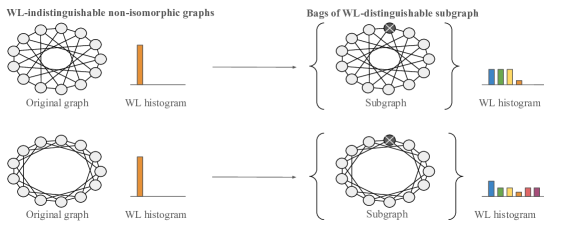
This raises the following question: is it really necessary to consider all the subgraphs in the bag? To answer this question, consider the two non-isomorphic graphs in Figure 1, which are indistinguishable by MPNNs. As demonstrated by prior work (Cotta et al., 2021), encoding such graphs as bags of subgraphs, each obtained by marking a single node, makes them distinguishable. However, as can be seen from the Figure, the usage of all subgraphs is unnecessary, and distinguishability can be achieved by considering only one subgraph per graph. Thus, from the standpoint of expressive power, Subgraph GNNs can distinguish between these graphs using constant-sized bags, rather than the -sized bags typically employed by existing methods.
The example in Figure 1 shows the potential of subgraph selection policies returning a small number of subgraphs. However, as all node-marked subgraphs in these two graphs are isomorphic, randomly selecting one subgraph in each graph is sufficient for disambiguation. In Proposition 3 we generalize this example and prove that there exist families of non-isomorphic graphs where a small number of carefully chosen subgraphs is sufficient and necessary for identifying otherwise WL-indistinguishable graphs. In these families, the probability that a random selection baseline returns the required subgraphs tends to zero, motivating the problem of learning to select subgraphs instead of randomly choosing them.
In this paper, we aim to learn subgraph selection policies, returning a significantly smaller number of subgraphs compared to the total available in the bag, in a task- and graph-adaptive fashion. To that end, we propose an architecture, dubbed Policy-learn, composed of two Subgraph GNNs: (i) a selection network, and (ii) a downstream prediction network. The selection network learns a subgraph selection policy and iteratively constructs a bag of subgraphs. This bag is then passed to the prediction network to solve the downstream task of interest. The complete architecture is trained in an end-to-end fashion according to the downstream task’s loss function, by leveraging the straight-through Gumbel-Softmax estimator (Jang et al., 2016; Maddison et al., 2017) to allow differentiable sampling from the selection policy.
As we shall see, our choice of using a Subgraph GNN as the selection network, as well as the sequential nature of our policy generation, provide additional expressive power compared to random selection and previous approaches (Qian et al., 2022) and allow us to learn a more diverse set of policies. Specifically, we prove that our framework can learn to select the subgraphs required for disambiguation in the families of graphs mentioned above, while previous approaches provably cannot do better than randomly selecting a subset of subgraphs.
Experimentally, we show that Policy-learn is competitive with full-bag Subgraph GNNs, even when learning to select a dramatically smaller number of subgraphs. Furthermore, we demonstrate its advantages over random selection baselines and previous methods on a wide range of tasks.
Contributions. This paper provides the following contributions: (1) A new framework for learning subgraph selection policies; (2) A theoretical analysis motivating the policy learning task as well as our architecture; and (3) An experimental evaluation of the new approach demonstrating its advantages.
2 Related Work
Expressive power limitations of GNNs. Multiple works have been proposed to overcome the expressive power limitations of MPNNs, which are constrained by the WL isomorphism test (Xu et al., 2019; Morris et al., 2019). Other than subgraph-based methods, which are the focus of this work, these approaches include: (1) Architectures aligned to the -WL hierarchy (Morris et al., 2019; 2020b; Maron et al., 2019b; a); (2) Augmentations of the node features with node identifiers (Abboud et al., 2020; Sato, 2020; Dasoulas et al., 2021; Murphy et al., 2019); (3) Models leveraging additional information, such as homomorphism and subgraph counts (Barceló et al., 2021; Bouritsas et al., 2022), graph polynomials (Puny et al., 2023), and simplicial and cellular complexes (Bodnar et al., 2021b; a). We refer the reader to the survey by Morris et al. (2021) for a review of different methods.
Subgraph GNNs. Despite the differences in the specific layer operations, the idea of constructing bags of subgraphs to be processed through message-passing layers has been recently proposed by several concurrent works. Cotta et al. (2021) proposed to first obtain subgraphs by deleting nodes in the original graph, and then apply an MPNN to each subgraph separately, whose representations are finally aggregated through a set function. Zhang & Li (2021) considered subgraphs obtained by constructing the local ego-network around each node in the graph, an approach also followed by Zhao et al. (2022), which further incorporates feature aggregation modules that aggregate node representations across different subgraphs. Bevilacqua et al. (2022) developed two classes of Subgraph GNNs, which differ in the symmetry group they are equivariant to: (i) DS-GNN, which processes each subgraph independently, and (ii) DSS-GNN, which includes feature aggregation modules in light of the alignment of nodes in different subgraphs. Huang et al. (2023); Yan et al. (2023); Papp & Wattenhofer (2022) further studied the expressive power of Subgraph GNNs, while Zhou et al. (2023) proposed a framework that encompasses several existing methods. Recently, Frasca et al. (2022); Qian et al. (2022) provided a theoretical analysis of node-based Subgraph GNNs, demonstrating that they are upper-bounded by 3-WL, while Zhang et al. (2023) presented a complete hierarchy of existing architectures with growing expressive power. Finally, other works such as Rong et al. (2019); Vignac et al. (2020); Papp et al. (2021); You et al. (2021) can be interpreted as Subgraph GNNs.
Most related to our work is the recent paper of Qian et al. (2022), which, to the best of our knowledge, presented the first framework that learns a subgraph selection policy rather than employing a full bag or a random selection policy. Our work differs from theirs in three main ways: (i) Bag of subgraphs construction: Our method generates the bag sequentially, compared to their one-shot generation; (ii) Expressive selection GNN architecture: We parameterize the selection network using a Subgraph GNN, that is more expressive than the MPNN used by Qian et al. (2022); (iii) Differentiable sampling mechanism: We use the well-known Gumbel-Softmax trick to enable gradient backpropagation through the discrete sampling process, while Qian et al. (2022) use I-MLE (Niepert et al., 2021); and (iv) Motivation: our work is primarily motivated by scenarios where a subset of subgraphs is sufficient for maximal expressive power, while Qian et al. (2022) aim to make higher-order generation policies (where each subgraph is generated from tuples of nodes) practical. We prove that our choices lead to a framework that can learn subgraph distributions that cannot be expressed with Qian et al. (2022), and demonstrate that our framework performs better on real-world datasets.
3 Problem Formulation
Let , be a node-attributed, undirected, simple graph with nodes, where represents the adjacency matrix of and is the node feature matrix. Given a graph , a Subgraph GNN first transforms into a bag (multiset) of subgraphs, , obtained from a predefined generation policy, where denotes subgraph . Then, it processes through a stacking of (node- and subgraph-) permutation equivariant layers, followed by a pooling function to obtain graph or node representations to be used for the final predictions.
In this paper, we focus on the node marking (NM) subgraph generation policy (Papp & Wattenhofer, 2022), where each subgraph is obtained by marking a single node in the graph, without altering the connectivity of the original graph111Although technically, NM does not generate subgraphs in the traditional sense, the marked versions of the original graph are commonly regarded as subgraphs (Papp & Wattenhofer, 2022).. More specifically, for each subgraph , there exists a node such that and , where denotes channel-wise concatenation and is a one-hot indicator vector for the node . We refer to the node as the root of , which we will equivalently denote as . Notably, since each subgraph is obtained by marking exactly one node, there is a bijection between nodes and subgraphs, making the total number of subgraphs under the NM policy equal to the number of nodes . Finally, we remark that we chose NM as the generation policy as it generalizes several other policies (Zhang et al., 2023). Any other node-based policy, preserving this bijection between nodes and subgraphs, can be equivalently considered.
Objective.
Motivated by their recent success, we would like to employ a Subgraph GNN to solve a given graph learning task (e.g., graph classification). Aiming to mitigate the computational overhead of using the full bag , we wish to propose a method for learning a subgraph selection policy that, given the input graph , returns a subset of to be used as an input to the Subgraph GNN in order to solve the downstream task at hand.
We denote by the output of , consisting of the original graph and selected subgraphs. That is, , where node in is the root node of .
4 Insights for the Subgraph Selection Learning Problem
In this section, we motivate the problem of learning to select subgraphs in the context of Subgraph GNNs. Specifically, we seek to address two research questions: (i) Are there subgraph selection policies that return small yet effective bags of subgraphs?, and (ii) How do these policies compare to strategies that uniformly sample a random subset of all possible subgraphs in the bag?. In the following, we present our main results, while details and proofs are provided in Appendix B.
Powerful policies containing only a single subgraph.
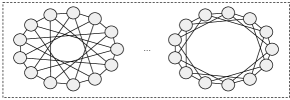
To address the first question, we consider Circulant Skip Links (CSL) graphs, an instantiation of which was shown in Figure 1 (CSL(, ) and CSL(, )).
Definition 1 (CSL graph (Murphy et al., 2019)).
Let , , be such that is co-prime with and . A CSL graph, CSL(, ) is an undirected graph with nodes labeled as , whose edges form a cycle and have skip links. That is, the edge set is defined by a cycle formed by for , and , along with skip links defined recursively by the sequence , with and .
While CSL graphs are WL-indistinguishable (Murphy et al., 2019), they become distinguishable when considering the full bag of node-marked subgraphs (Cotta et al., 2021). Furthermore, since all subgraphs in the bag are isomorphic, it is easy to see that distinguishability is obtained even when considering a single subgraph per graph. This observation motivates the usage of small bags, as there exist cases where the expressive power of the full bag can be obtained with a very small subset of subgraphs.
The extreme case of CSL graphs, however, is too simplistic: randomly selecting one subgraph in each graph is sufficient for disambiguation. This leads to our second question, and, in the following, we build upon CSL graphs to define a family of graphs where random policies are not effective. As we shall see next, in these families only specific small subgraph selections lead to complete identification of the isomorphism type of each graph.
Families of graphs that require specific selections of subgraphs.
We obtain our family of graphs starting from CSL graphs, which we use as building blocks to define an -CSL graph.
Definition 2 (-CSL graph).
A -CSL graph, denoted as -CSL(, , is a graph with nodes obtained from disconnected non-isomorphic CSL (sub-)graphs with nodes, CSL(, ), . Note that the maximal value of depends on .
Our interest in these graphs lies in the fact that the family of non-isomorphic -CSL graphs contains WL-indistinguishable graphs, as we show in the following.
Theorem 1 (-CSL graphs are WL-indistinguishable).
Let be the family of non-isomorphic -CSL graphs (Definition 2). All graphs in are WL-indistinguishable.
While these graphs are WL-indistinguishable, we can distinguish all pairs when utilizing the full bag of node-marked subgraphs. More importantly, the full bag allows us to fully identify the isomorphism type of all graphs within the family, which implies the distinguishability of pairs of graphs. As we show next, it is however unnecessary to consider the entire bag of all the subgraphs. Instead, there exists a subgraph selection policy that returns only subgraphs, a significantly smaller number than the total in the full bag, which are provably sufficient for identifying the isomorphism type of all graphs within the family. This identification is attained when the root nodes of all subgraphs belong to different CSL (sub-)graphs. Furthermore, we prove that this condition is not only sufficient but also necessary. In other words, the isomorphism-type identification of all graphs within the family only occurs when there is at least one node-marked subgraph obtained from each CSL (sub-)graph.
Proposition 2 (There exists an efficient that fully identifies -CSL graphs).
Let be the family of non-isomorphic -CSL graphs (Definition 2). A node-marking based subgraph selection policy can identify the isomorphism type of any graph in if and only if its bag has a marking in each CSL (sub-)graph.
The above results demonstrate the existence of efficient and more sophisticated subgraph selection policies that enable the identification of isomorphism types. Remarkably, these can return bags as small as containing subgraphs, as long as each of them is obtained by marking a node in a different CSL (sub-)graph. The insight derived from the necessary condition is equally profound: a random selection approach, which uniformly samples subgraphs per graph, does not ensure identification of the isomorphism type, because the subgraphs might not be drawn from distinct CSL (sub-)graphs. This finding highlights the sub-optimality of random selection strategies, as we formalize below.
Proposition 3 (A random policy cannot efficiently identify -CSL graphs).
Let be any graph in the family of non-isomorphic -CSL graphs, namely (Definition 2). The probability that a random policy, which uniformly samples subgraphs from the full bag, can successfully identify the isomorphism type of is , which tends to 0 as increases.
The above result has important implications for Subgraph GNNs when coupled with random policies. It indicates that Subgraph GNNs combined with a random subgraph selection policy, are unlikely to identify the isomorphism type of , assuming the number of sampled subgraphs is . In Lemma 6 in Appendix B, we further show that the expected number of subgraphs that a random policy must uniformly draw before identification is . Notably, this number is significantly larger than the minimum number of subgraphs required by . For instance, when , a random policy would have to sample around subgraphs per graph. This is more than four times the number of subgraphs returned by , making it clear that there exists a substantially more effective approach than random sampling to the problem.
5 Method
The following section describes the proposed framework: Policy-learn. We start with an overview of the method, before discussing in detail the specific components, namely the selection and the prediction networks, as well as the learning procedure used to differentiate through the discrete sampling process.
5.1 Overview
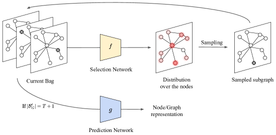
Our method is illustrated in Figure 3 and described in Algorithm 1. It is composed of two main Subgraph GNNs: a subgraph selection network, denoted as , that generates the subgraph selection policy , and a downstream prediction network, denoted as , that solves the learning task of interest. More concretely, given an input graph , we initialize the bag of subgraphs with the original graph, . Then, at each step , the selection network takes the current bag of subgraphs as input and outputs an un-normalized distribution , defined over the nodes of the original graph . Our algorithm samples from to select a node that will serve as the root of the next subgraph . This new subgraph is added to the bag, i.e. we define . After subgraph selections, where is a hyperparameter representing the number of subgraphs in the bag ( considering the original graph), the final bag is passed to the prediction network , a Subgraph GNN designed to solve the downstream task at hand. Both and are trained jointly in an end-to-end manner, and we use the Gumbel-Softmax trick (Jang et al., 2016; Maddison et al., 2017) to backpropagate through the discrete sampling process. In what follows, we elaborate on the exact implementation and details of each component of our approach.
5.2 Subgraph Selection Network
The goal of is to output a distribution over the nodes of the original graph, determining which node should serve as the root of the next subgraph that will be added to the bag. As this network takes a bag of subgraphs as its input, it is natural to implement as a Subgraph GNN. Specifically, we employ the most efficient Subgraph GNN variant, namely DS-GNN (Cotta et al., 2021; Bevilacqua et al., 2022), that performs message-passing operations on each subgraph independently using an MPNN, referred to as the subgraph encoder. Subsequently, it applies a pooling operation across the subgraphs in the bag, to obtain a single representation for each node in the input graph .
Since we have both the original node features and the markings, the subgraph encoder in our DS-GNN architecture is implemented using the model proposed by Dwivedi et al. (2021), which decouples the two representations to improve learning. This encoder consists of two message-passing functions: , responsible for updating the markings, and , responsible for updating the original features. Formally, at the -th iteration, we are provided with a bag of subgraphs of size . For each subgraph , we compute the following for where represents the total number of layers in the selection network:
| (1a) | ||||
| (1b) | ||||
with and the -th message passing layers in and , respectively. At , we initialize the marking as and the input node features as .
After the -th layer, we combine the marking and node features to obtain the updated node features, as follows:
| (2) |
Note that in this way we obtain node features for every subgraph in the bag. In order to unify them into a single output per node, we pool the node features along the subgraph dimension. We then apply an MLP that reduces the channel dimension to one, to obtain the following un-normalized node probabilities from which we sample the next root node:
| (3) |
Backpropagating through the sampling process.
A naive sampling strategy is not differentiable and therefore will prevent us from backpropagating gradients to update the weights of the selection network . Therefore, we use the straight-through Gumbel-Softmax estimator (Jang et al., 2016; Maddison et al., 2017) to sample from , and obtain the one-hot encoding marking of the next subgraph to be added to the current bag of subgraphs:
| (4) |
We denote the subgraph associated with the node marking by . Therefore, the bag of subgraphs at the -th iteration reads .
5.3 Downstream Prediction Network
Similarly to the selection network , our prediction network is parameterized as a Subgraph GNN. It takes as input the final bag of subgraphs that was sampled using , and produces graph- or node-level predictions depending on the task of interest. Like the selection network, we employ a DS-GNN architecture and implement the subgraph encoder using two message-passing functions, and , with layers and updates identical to Equations 1a and 1b. Note that, while and are architecturally similar, they are two different networks with their own set of learnable weights. In the first layer, i.e., , we set the initial marking as and input node features as , where we use the bar, i.e., , , to denote the representations in the downstream prediction model and distinguish them from the ones in the selection model.
After the -th layer, we combine the marking and node features to obtain the updated node features and pool the node features along the subgraph and potentially the node dimension to obtain a final node or graph representation. This representation is then further processed with an MLP to obtain the final prediction.
6 Theoretical Analysis
In this section, we study the theoretical capabilities of our framework, focusing on its ability to provably identify the isomorphism type of the -CSL graphs introduced in Proposition 3. Due to space constraints, all proofs are relegated to Appendix B. We start by showing that, differently than random selection approaches, Policy-learn can identify the isomorphism type of any -CSL graph (Definition 2) when learning to select only subgraphs. Remarkably, this number is significantly smaller than the total subgraphs in the full bag, as well as the expected number of subgraphs required by a random policy.
Theorem 4 (Policy-learn can identify ).
Let be any graph in the family of non-isomorphic -CSL graphs, namely (Definition 2). There exist weights of and such that Policy-learn with can identify the isomorphism type of within the family.
The idea of the proof lies in the ability of the selection network within Policy-learn to implement a policy that returns subgraphs per graph where: (i) each subgraph is obtained by marking exactly one node and (ii) each marked node belongs to a different CSL (sub-)graph. Given that this policy serves as a sufficient condition for the identification of the isomorphism types (Proposition 2), our proposed framework successfully inherits this ability. More specifically, the proof (in Appendix B) proceeds by showing that the selection network can always distinguish all the nodes belonging to already-marked CSL (sub-)graphs from the rest, and therefore can assign them a zero probability of being sampled, while maintaining a uniform probability on all the remaining nodes.
The previous result further sets our method apart from the OSAN method proposed in Qian et al. (2022). Indeed, as its selection network is parameterized as an MPNN, and given that contains WL-indistinguishable graphs composed by WL-indistinguishable CSL (sub-)graphs, then OSAN cannot differentiate between all the nodes in the graph. Therefore, since all the subgraphs are selected simultaneously rather than sequentially, the resulting sampling process is the same as uniform sampling. Consequently, it cannot ensure that marked nodes belong to different CSL (sub-)graphs. Since this condition is not only sufficient but also necessary for the identification of the isomorphism type (Proposition 2), OSAN effectively behaves like a random policy for indistinguishable graphs.
Theorem 5 (Qian et al. (2022) cannot efficiently identify ).
Let be any graph in the family of non-isomorphic -CSL graphs, namely (Definition 2). Then, the probability that OSAN (Qian et al., 2022) with subgraphs can successfully identify the isomorphism type of is , which tends to 0 as increases.
Up until this point, our focus has been on demonstrating that Policy-learn has the capability to implement the policy for identification within . However, it is important to note that is not the sole policy that Policy-learn can implement. Indeed, Policy-learn can also learn subgraph selection policies that depend on the local graph structure, such as the policy returning all subgraphs with root nodes having degree greater than a specified threshold (see Proposition 7 in Appendix B).
7 Experiments
In this section, we empirically investigate the performance of Policy-learn. In particular, we seek to answer the following questions: (1) Can our approach consistently outperform MPNNs, as demonstrated by full-bag Subgraph GNNs? (2) Does Policy-learn achieve better performance than a random baseline that uniformly samples a subset of subgraphs at each training epoch? (3) How does our method compare to the existing learnable selection strategy OSAN (Qian et al., 2022)? (4) Is our approach competitive to full-bag Subgraph GNNs on real-world datasets?
In the following, we present our main results and refer to Appendix C for details. For each task, we include two baselines: Random, which represents the random subgraph selection, and Full, which corresponds to the full-bag approach. These baselines utilize the same downstream prediction network (appropriately tuned) as Policy-learn, with Random selecting random subsets of subgraphs equal in size to those used by Policy-learn (denoted by ), and Full employing the entire bag.
| Method | ZINC (MAE ) |
|---|---|
| GCN (Kipf & Welling, 2017) | 0.3210.009 |
| GIN (Xu et al., 2019) | 0.1630.004 |
| PNA (Corso et al., 2020) | 0.1330.011 |
| GSN (Bouritsas et al., 2022) | 0.1010.010 |
| CIN (Bodnar et al., 2021a) | 0.0790.006 |
| OSAN (Qian et al., 2022) | 0.1770.016 |
| Full | 0.0870.003 |
| Random | 0.1360.005 |
| Policy-learn | 0.1200.003 |
| Random | 0.1130.006 |
| Policy-learn | 0.1090.005 |
ZINC. We experimented with the ZINC-12k molecular dataset (Sterling & Irwin, 2015; Gómez-Bombarelli et al., 2018; Dwivedi et al., 2020), where as prescribed we maintain a 500k parameter budget. As can be seen from Table 1, Policy-learn significantly improves over OSAN, and surpasses the random baseline. Notably, OSAN performs worse than our random baseline due to differences in the implementation of the prediction network. As expected, the gap between Policy-learn and Random is larger when the number of subgraphs is smaller, where selecting the most informative subgraphs is more crucial. Additional comparisons to existing full-bag Subgraph GNNs can be found in Table 5 in Appendix C.
| Method | RDT-B (ACC ) |
|---|---|
| GIN (Xu et al., 2019) | 92.42.5 |
| SIN (Bodnar et al., 2021b) | 92.21.0 |
| CIN (Bodnar et al., 2021a) | 92.42.1 |
| Full | OOM |
| Random | 92.61.5 |
| Random | 92.41.0 |
| Policy-learn | 93.00.9 |
Reddit. To showcase the capabilities of Policy-learn on large graphs, we experimented with the Reddit-Binary dataset (Morris et al., 2020a) where full-bag Subgraph GNNs cannot be otherwise applied due to the high average number of nodes, and consequently subgraphs, per graph (). Policy-learn exhibits the best performance among all efficient baselines (Table 2), while maintaining competitive inference runtimes (Table 7 in Appendix C), opening up the applicability of Subgraph GNNs to unexplored avenues. Table 6 in Appendix C further compares to random baselines coupled with different subgraph-based downstream models.
| Method / Dataset | molesol | moltox21 | molbace | molhiv |
|---|---|---|---|---|
| RMSE | ROC-AUC | ROC-AUC | ROC-AUC | |
| GCN (Kipf & Welling, 2017) | 1.1140.036 | 75.290.69 | 79.151.44 | 76.060.97 |
| GIN (Xu et al., 2019) | 1.1730.057 | 74.910.51 | 72.974.00 | 75.581.40 |
| OSAN (Qian et al., 2022) | 0.9840.086 | N/A | 72.306.60 | N/A |
| Full | 0.8470.015 | 76.251.12 | 78.411.94 | 76.541.37 |
| Random | 0.9510.039 | 76.650.89 | 75.364.28 | 77.551.24 |
| Policy-learn | 0.8770.029 | 77.470.82 | 78.402.85 | 79.130.60 |
| Random | 0.9000.032 | 76.620.63 | 78.142.36 | 77.302.56 |
| Policy-learn | 0.8830.032 | 77.360.60 | 78.392.28 | 78.491.01 |
OGB. We tested our framework on several datasets from the OGB benchmark collection (Hu et al., 2020). Table 3 shows the performances of our method when compared to MPNNs and efficient subgraph selection policies. For OSAN, we report the best result across all node-based policies, which is obtained with a larger number of subgraphs than what we consider ( compared to our ). Notably, Policy-learn improves over MPNNs while retaining similar asymptotic complexity, and consistently outperforms OSAN and Random. The performance gap between Policy-learn and Random is more significant with , particularly on molesol and molbace. Remarkably, Policy-learn approaches the full-bag baseline Full on molesol and molbace, and even outperforms it on moltox21 and molhiv, achieving the highest score. These results can be attributed to the generalization challenges posed by the dataset splits, which are further confirmed by the observation that increasing the number of subgraphs does not improve results. Table 4 in Appendix C additionally reports the results of existing full-bag Subgraph GNNs.
8 Conclusions
In this paper we introduced a novel framework, Policy-learn, for learning to select a small subset of the large set of possible subgraphs in order to reduce the computational overhead of Subgraph GNNs. We addressed the pivotal question of whether a small, carefully selected, subset of subgraphs can be used to identify the isomorphism type of graphs that would otherwise be WL-indistinguishable. We proved that, unlike random selections and previous work, our method can provably learn to select these critical subgraphs. Empirically, we demonstrated that Policy-learn consistently outperforms random selection strategies and approaches the performance of full-bag methods. Furthermore, it significantly surpasses prior work addressing the same problem, across all the datasets we considered. This underscores the effectiveness of our framework in focusing on the necessary subgraphs, mitigating computational complexity, and achieving competitive results. We believe our approach opens the door to broader applications of Subgraph GNNs.
Acknowledgments
BR acknowledges support from the National Science Foundation (NSF) awards CAREER IIS-1943364 and CNS-2212160, an Amazon Research Award, AnalytiXIN, and the Wabash Heartland Innovation Network (WHIN). HM is the Robert J. Shillman Fellow, and is supported by the Israel Science Foundation through a personal grant (ISF 264/23) and an equipment grant (ISF 532/23). Any opinions, findings and conclusions or recommendations are those of the authors and do not necessarily reflect the views of the sponsors.
References
- Abboud et al. (2020) Ralph Abboud, İsmail İlkan Ceylan, Martin Grohe, and Thomas Lukasiewicz. The surprising power of graph neural networks with random node initialization. In Proceedings of the Thirtieth International Joint Conference on Artificial Intelligence (IJCAI), 2020.
- Barceló et al. (2021) Pablo Barceló, Floris Geerts, Juan Reutter, and Maksimilian Ryschkov. Graph neural networks with local graph parameters. Advances in Neural Information Processing Systems, 34:25280–25293, 2021.
- Bevilacqua et al. (2022) Beatrice Bevilacqua, Fabrizio Frasca, Derek Lim, Balasubramaniam Srinivasan, Chen Cai, Gopinath Balamurugan, Michael M Bronstein, and Haggai Maron. Equivariant subgraph aggregation networks. In International Conference on Learning Representations, 2022.
- Biewald (2020) Lukas Biewald. Experiment tracking with weights and biases, 2020. Software available from wandb.com.
- Blom et al. (1993) Gunnar Blom, Lars Holst, and Dennis Sandell. Problems and Snapshots from the World of Probability. Springer Science & Business Media, 1993.
- Bodnar et al. (2021a) Cristian Bodnar, Fabrizio Frasca, Nina Otter, Yuguang Wang, Pietro Liò, Guido F Montúfar, and Michael Bronstein. Weisfeiler and lehman go cellular: Cw networks. In Advances in Neural Information Processing Systems, volume 34, 2021a.
- Bodnar et al. (2021b) Cristian Bodnar, Fabrizio Frasca, Yuguang Wang, Nina Otter, Guido F Montúfar, Pietro Liò, and Michael Bronstein. Weisfeiler and lehman go topological: Message passing simplicial networks. In International Conference on Machine Learning, 2021b.
- Bouritsas et al. (2022) Giorgos Bouritsas, Fabrizio Frasca, Stefanos P Zafeiriou, and Michael Bronstein. Improving graph neural network expressivity via subgraph isomorphism counting. IEEE Transactions on Pattern Analysis and Machine Intelligence, 2022.
- Chen et al. (2019) Guangyong Chen, Pengfei Chen, Chang-Yu Hsieh, Chee-Kong Lee, Benben Liao, Renjie Liao, Weiwen Liu, Jiezhong Qiu, Qiming Sun, Jie Tang, Richard Zemel, and Shengyu Zhang. Alchemy: A quantum chemistry dataset for benchmarking ai models. arXiv preprint arXiv:1906.09427, 2019.
- Corso et al. (2020) Gabriele Corso, Luca Cavalleri, Dominique Beaini, Pietro Liò, and Petar Veličković. Principal neighbourhood aggregation for graph nets. In Advances in Neural Information Processing Systems, volume 33, 2020.
- Cotta et al. (2021) Leonardo Cotta, Christopher Morris, and Bruno Ribeiro. Reconstruction for powerful graph representations. In Advances in Neural Information Processing Systems, volume 34, 2021.
- Dasoulas et al. (2021) George Dasoulas, Ludovic Dos Santos, Kevin Scaman, and Aladin Virmaux. Coloring graph neural networks for node disambiguation. In Proceedings of the Twenty-Ninth International Conference on International Joint Conferences on Artificial Intelligence, pp. 2126–2132, 2021.
- Dwivedi et al. (2020) Vijay Prakash Dwivedi, Chaitanya K Joshi, Thomas Laurent, Yoshua Bengio, and Xavier Bresson. Benchmarking graph neural networks. arXiv preprint arXiv:2003.00982, 2020.
- Dwivedi et al. (2021) Vijay Prakash Dwivedi, Anh Tuan Luu, Thomas Laurent, Yoshua Bengio, and Xavier Bresson. Graph neural networks with learnable structural and positional representations. In International Conference on Learning Representations, 2021.
- Fey & Lenssen (2019) Matthias Fey and Jan Eric Lenssen. Fast graph representation learning with pytorch geometric. arXiv preprint arXiv:1903.02428, 2019.
- Frasca et al. (2022) Fabrizio Frasca, Beatrice Bevilacqua, Michael M Bronstein, and Haggai Maron. Understanding and extending subgraph gnns by rethinking their symmetries. In Advances in Neural Information Processing Systems, 2022.
- Gómez-Bombarelli et al. (2018) Rafael Gómez-Bombarelli, Jennifer N. Wei, David Duvenaud, José Miguel Hernández-Lobato, Benjamín Sánchez-Lengeling, Dennis Sheberla, Jorge Aguilera-Iparraguirre, Timothy D. Hirzel, Ryan P. Adams, and Alán Aspuru-Guzik. Automatic chemical design using a data-driven continuous representation of molecules. ACS Central Science, 4(2):268–276, Jan 2018.
- Hu et al. (2020) Shengding Hu, Zheng Xiong, Meng Qu, Xingdi Yuan, Marc-Alexandre Côté, Zhiyuan Liu, and Jian Tang. Graph policy network for transferable active learning on graphs. Advances in Neural Information Processing Systems, 33:10174–10185, 2020.
- Huang et al. (2023) Yinan Huang, Xingang Peng, Jianzhu Ma, and Muhan Zhang. Boosting the cycle counting power of graph neural networks with I2-GNNs. International Conference on Learning Representations, 2023.
- Jang et al. (2016) Eric Jang, Shixiang Gu, and Ben Poole. Categorical reparameterization with gumbel-softmax. In International Conference on Learning Representations, 2016.
- Kipf & Welling (2017) Thomas N Kipf and Max Welling. Semi-supervised classification with graph convolutional networks. In International Conference on Learning Representations, 2017.
- Maddison et al. (2017) C Maddison, A Mnih, and Y Teh. The concrete distribution: A continuous relaxation of discrete random variables. In Proceedings of the international conference on learning Representations. International Conference on Learning Representations, 2017.
- Maron et al. (2019a) Haggai Maron, Heli Ben-Hamu, Hadar Serviansky, and Yaron Lipman. Provably powerful graph networks. In Advances in Neural Information Processing Systems, volume 32, 2019a.
- Maron et al. (2019b) Haggai Maron, Heli Ben-Hamu, Nadav Shamir, and Yaron Lipman. Invariant and equivariant graph networks. In International Conference on Learning Representations, 2019b.
- Martinkus et al. (2023) Karolis Martinkus, Pál András Papp, Benedikt Schesch, and Roger Wattenhofer. Agent-based graph neural networks. In International Conference on Learning Representations (ICLR). arXiv, 2023.
- Meirom et al. (2021) Eli Meirom, Haggai Maron, Shie Mannor, and Gal Chechik. Controlling graph dynamics with reinforcement learning and graph neural networks. In International Conference on Machine Learning, pp. 7565–7577. PMLR, 2021.
- Mitzenmacher & Upfal (2017) Michael Mitzenmacher and Eli Upfal. Probability and computing: Randomization and probabilistic techniques in algorithms and data analysis. Cambridge university press, 2017.
- Morris et al. (2019) Christopher Morris, Martin Ritzert, Matthias Fey, William L Hamilton, Jan Eric Lenssen, Gaurav Rattan, and Martin Grohe. Weisfeiler and leman go neural: Higher-order graph neural networks. In Proceedings of the AAAI conference on artificial intelligence, volume 33, pp. 4602–4609, 2019.
- Morris et al. (2020a) Christopher Morris, Nils M. Kriege, Franka Bause, Kristian Kersting, Petra Mutzel, and Marion Neumann. Tudataset: A collection of benchmark datasets for learning with graphs. In ICML 2020 Workshop on Graph Representation Learning and Beyond (GRL+ 2020), 2020a.
- Morris et al. (2020b) Christopher Morris, Gaurav Rattan, and Petra Mutzel. Weisfeiler and leman go sparse: Towards scalable higher-order graph embeddings. In Advances in Neural Information Processing Systems, volume 33, 2020b.
- Morris et al. (2021) Christopher Morris, Yaron Lipman, Haggai Maron, Bastian Rieck, Nils M Kriege, Martin Grohe, Matthias Fey, and Karsten Borgwardt. Weisfeiler and leman go machine learning: The story so far. arXiv preprint arXiv:2112.09992, 2021.
- Murphy et al. (2019) Ryan Murphy, Balasubramaniam Srinivasan, Vinayak Rao, and Bruno Ribeiro. Relational pooling for graph representations. In International Conference on Machine Learning, pp. 4663–4673. PMLR, 2019.
- Niepert et al. (2021) Mathias Niepert, Pasquale Minervini, and Luca Franceschi. Implicit mle: backpropagating through discrete exponential family distributions. Advances in Neural Information Processing Systems, 34:14567–14579, 2021.
- Papp & Wattenhofer (2022) Pál András Papp and Roger Wattenhofer. A theoretical comparison of graph neural network extensions. In International Conference on Machine Learning, pp. 17323–17345. PMLR, 2022.
- Papp et al. (2021) Pál András Papp, Karolis Martinkus, Lukas Faber, and Roger Wattenhofer. Dropgnn: Random dropouts increase the expressiveness of graph neural networks. Advances in Neural Information Processing Systems, 34:21997–22009, 2021.
- Paszke et al. (2019) Adam Paszke, Sam Gross, Francisco Massa, Adam Lerer, James Bradbury, Gregory Chanan, Trevor Killeen, Zeming Lin, Natalia Gimelshein, Luca Antiga, Alban Desmaison, Andreas Kopf, Edward Yang, Zachary DeVito, Martin Raison, Alykhan Tejani, Sasank Chilamkurthy, Benoit Steiner, Lu Fang, Junjie Bai, and Soumith Chintala. Pytorch: An imperative style, high-performance deep learning library. In Advances in Neural Information Processing Systems, volume 32, 2019.
- Puny et al. (2023) Omri Puny, Derek Lim, Bobak Kiani, Haggai Maron, and Yaron Lipman. Equivariant polynomials for graph neural networks. In International Conference on Machine Learning, pp. 28191–28222. PMLR, 2023.
- Qian et al. (2022) Chendi Qian, Gaurav Rattan, Floris Geerts, Christopher Morris, and Mathias Niepert. Ordered subgraph aggregation networks. In Advances in Neural Information Processing Systems, volume 35, 2022.
- Qian et al. (2023) Chendi Qian, Andrei Manolache, Kareem Ahmed, Zhe Zeng, Guy Van den Broeck, Mathias Niepert, and Christopher Morris. Probabilistically rewired message-passing neural networks, 2023.
- Rong et al. (2019) Yu Rong, Wenbing Huang, Tingyang Xu, and Junzhou Huang. Dropedge: Towards deep graph convolutional networks on node classification. In International Conference on Learning Representations, 2019.
- Sato (2020) Ryoma Sato. A survey on the expressive power of graph neural networks. arXiv preprint arXiv:2003.04078, 2020.
- Sterling & Irwin (2015) Teague Sterling and John J. Irwin. ZINC 15 – ligand discovery for everyone. Journal of Chemical Information and Modeling, 55(11):2324–2337, 11 2015. doi: 10.1021/acs.jcim.5b00559.
- Vignac et al. (2020) Clement Vignac, Andreas Loukas, and Pascal Frossard. Building powerful and equivariant graph neural networks with structural message-passing. Advances in neural information processing systems, 33:14143–14155, 2020.
- Xu et al. (2019) Keyulu Xu, Weihua Hu, Jure Leskovec, and Stefanie Jegelka. How powerful are graph neural networks? In International Conference on Learning Representations, 2019.
- Yan et al. (2023) Zuoyu Yan, Junru Zhou, Liangcai Gao, Zhi Tang, and Muhan Zhang. Efficiently counting substructures by subgraph gnns without running gnn on subgraphs. arXiv preprint arXiv:2303.10576, 2023.
- You et al. (2021) Jiaxuan You, Jonathan M Gomes-Selman, Rex Ying, and Jure Leskovec. Identity-aware graph neural networks. In Proceedings of the AAAI Conference on Artificial Intelligence, volume 35, pp. 10737–10745, 2021.
- Zhang et al. (2023) Bohang Zhang, Guhao Feng, Yiheng Du, Di He, and Liwei Wang. A complete expressiveness hierarchy for subgraph gnns via subgraph weisfeiler-lehman tests. In International Conference on Machine Learning, 2023.
- Zhang & Li (2021) Muhan Zhang and Pan Li. Nested graph neural networks. In Advances in Neural Information Processing Systems, volume 34, 2021.
- Zhao et al. (2022) Lingxiao Zhao, Wei Jin, Leman Akoglu, and Neil Shah. From stars to subgraphs: Uplifting any GNN with local structure awareness. In International Conference on Learning Representations, 2022.
- Zhou et al. (2023) Cai Zhou, Xiyuan Wang, and Muhan Zhang. From relational pooling to subgraph gnns: A universal framework for more expressive graph neural networks. In International Conference on Machine Learning, 2023.
Appendix A Additional Related Work
Our approach is related not only to Subgraph GNNs and expressive GNN architecture, as discussed in the main paper, but also to other sampling strategies in the graph domain. In the context of active learning, Hu et al. (2020) propose a reinforcement learning approach that learns which subset of nodes to label in order to reduce the annotation cost of training GNNs. For controlling the dynamics of a system using localized interventions, Meirom et al. (2021) employ a reinforcement learning agent that selects a subset of nodes at each step and attempts to change their state, with an objective that depends on the number of nodes in each state. More similar to our sampling strategy is the work by Martinkus et al. (2023) which proposes a GNN architecture augmented with neural agents, that traverse the graph and then collectively classify it. Notably, at each step, an agent chooses a neighboring node to transition to using the Gumbel-Softmax trick.
Appendix B Proofs
This appendix includes the proofs for the theoretical results presented in Propositions 3 and 5. We start by formally proving that the family of non-isomorphic -CSL graphs, defined in Definition 2, contains WL-indistinguishable graphs.
See 1
Proof.
Let , be any two -CSL graphs in . We will prove that , are WL-indistinguishable by simulating one WL round starting from a constant color initialization.
-
(Iter. 1)
The colors after the first iteration represent the node degrees. Since each node has degree (because it belongs to one CSL (sub-)graph), then all nodes will have the same color.
Since the colors after the first iterations are a finer refinement of the initialization colors, the algorithm stops and the graphs are not separated. ∎
Next, we show that there exists an efficient policy , that can return as few subgraphs as , providing strong guarantees. Indeed, represents a necessary and sufficient condition for identifying the isomorphism type of all graphs in , as we prove next. See 2
Proof.
We will prove the two cases separately.
Sufficiency. Consider any graph , and let be a subgraph returned by obtained by marking any node in the -th CSL (sub-)graph of graph . Note that is sufficient to identify the isomorphism type of the -th CSL (sub-)graph, because marking any node is sufficient for disambiguation of any possible pair of CSL graphs (Cotta et al., 2021, Theorem 2). Consider the set of histograms, each obtained by marking a different CSL (sub-)graph. Note that if returns more than subgraphs, then identical histograms indicate that the corresponding subgraphs are obtained from the same CSL (sub-)graph, because is composed by non-isomorphic CSL (sub-)graphs. Thus, identical histograms can be simply discarded when constructing . Then, the set is sufficient to identify the isomorphism type of , as each element of identifies one of its CSL (sub-)graphs.
Necessity. The proof proceeds by contrapositive. Consider a policy and assume that there exists at least one CSL (sub-)graph such that none of the marked nodes belongs to it. Without loss of generality, assume that only one CSL (sub-)graphs is not covered, meaning no marked nodes belong to it. Then, cannot identify the isomorphism type of , because it is unaware of the isomorphism type of the CSL (sub-)graph that is not covered. More precisely, consider a graph such that: (1) is non-isomorphic to and (2) differ from only in one CSL (sub-)graph, which is the one not covered by . Then, cannot identify whether the isomorphism type of its input is the one of or the one of . ∎
The above theorem implies that a random selection baselines might fail to select the subgraphs required for the identification, as it might fail to draw at least one subgraph from each CSL (sub-)graph. In the following we prove that the implications are even more severe as grows. See 3
Proof.
From Proposition 2, each of the subgraphs must be generated by marking a node belonging to a different CSL (sub-)graph for the identification of the isomorphism type (necessary condition). Recall that the total number of CSL (sub-)graphs is , and each CSL (sub-)graph has exactly nodes. Thus, the probability of choosing nodes from different CSL (sub-)graphs is . Finally, since , the probability goes to zero as grows. ∎
Importantly, we derive the expected number of subgraphs that a random policy has to draw before identification.
Lemma 6.
Let be any graph in the family of non-isomorphic -CSL graphs, namely (Definition 2). The expected number of subgraphs that a random policy must uniformly draw before identification is .
Proof.
Note that we have an instance of the coupon collector problem. The proof follows the steps in Mitzenmacher & Upfal (2017); Blom et al. (1993). Let be the time to collect (any node from) the -th CSL (sub-)graphs, after CSL (sub-)graphs have already been collected by drawing at least one of their nodes for marking. Let be probability of collecting a new CSL (sub-)graph (one from which nodes where not drawn before). Then,
Therefore, has geometric distribution with expectation . By linearity of expectation, then the number of draws needed to collect all CSL (sub-)graphs is:
where is the harmonic number, which asymptotically grows as . Thus, we obtain the expectation . ∎
Our next theorem shows that Policy-learn does not suffer from the shortcomings of the random selection. Indeed, Policy-learn can provably implement the in Proposition 2, which in turn implies that it can learn to identify the isomorphism type of any graph in . See 4
Proof.
We will show that Policy-learn can implement the subgraph selection policy which returns subgraphs such that: (i) each subgraph is obtained by marking exactly one node and (ii) each marked node belongs to a different CSL (sub-)graph. Since is sufficient for identification (Proposition 2), then Policy-learn can provably identify the isomorphism type of .
Recall that we initialize the bag of subgraphs as . At step , since all nodes are WL-indistinguishable (see proof of Theorem 1), then is a uniform distribution. Thus, is randomly sampled from the possible nodes, and the bag is updated as . At step , we obtain a distribution over the nodes as . Assuming has enough layers (it is sufficient that the total number of layers is ), then all nodes belonging to the CSL (sub-)graph of node will have a different color than the remaining nodes. Therefore the MLP in Equation 3 can map them to have zero probability. On the contrary, the remaining nodes will all have the same color, and the MLP will map them to have the same probability. Thus will be uniform over all the nodes in the CSL (sub-)graphs other than the one containing node . Therefore, is randomly sampled from a CSL (sub-)graph different than one containing . By repeating the argument, we have that at each iteration Policy-learn samples one node from a CSL (sub-)graph that has not yet been selected. Thus, at the bag of subgraphs will contain all the subgraphs that are sufficient for identification. ∎
On the contrary, since OSAN (Qian et al., 2022) uses an MPNN as a selection network and samples all subgraphs at once, then it cannot perform better than randomly selecting subgraphs for the graphs in . See 5
Proof.
Recall that the selection network in OSAN is parameterized as an MPNN taking as input the original graph and returning as output probability distributions over the nodes, one for each of the subgraphs to sample. Since all nodes in are WL-indistinguishable (see proof of Theorem 1), then each of the probability distribution is uniform over the nodes. Therefore, each node is sampled uniformly at random. Since the sampled nodes must belong to different CSL (sub-)graphs for identification (Proposition 2), and because the probability of sampling nodes each belonging to a different CSL (sub-)graph from the uniform distribution is (Proposition 3), then the probability that OSAN can identify the isomorphism type of is . ∎
Finally, we prove that Policy-learn can return all and only subgraphs having as root a node with degree greater than a predefined number.
Proposition 7 (Policy-learn can implement degree-aware policies).
Consider a policy that returns all node-marked subgraphs whose root nodes have degree greater than a predefined , with . Then, Policy-learn can implement with .
Proof.
We will prove that we can implement degree-aware policies by showing that it exists a set of weights such that Policy-learn gives a uniform probability to all nodes with degree that have not been already selected. Since the selection network is iteratively applied for times, then Policy-learn would have selected all subgraphs after the last iteration.
Recall that we initialize the bag of subgraphs as , and, at any step, we sample a node and add the corresponding subgraph to the bag. In the following, we drop the dependency on both the graph and the step in the notation, and call the current bag simply by .
Since we are only interested in sampling subgraphs having root nodes with degree , we do not assume the presence of any additional initial node feature, and we directly work with a DS-GNN architecture with GraphConv encoders (Morris et al., 2019).222The extension to the presence of additional node features, as well as the usage of the separate propagation of them as in Dwivedi et al. (2021) is straightforward, and can be done by considering those additional weights as zeroed out. The representation for node in subgraph given by the -th layer of our selection network can be written as:
| (5) |
where with if is not the root of subgraph , and if is the root of subgraph . Recall that, given the representations for each node in each subgraph in the bag, we then obtain a distribution over the nodes in the original graph by simply pooling the final node representations at the final layer , across all the subgraphs, i.e., the unnormalized node distribution is obtained as:
| (6) |
We consider a selection Subgraph GNN with 4 layers (i.e., ), and ReLU non-linearities. Each layer will have two channels, one used to compute an indicator variable storing whether a node has degree greater than , and the other one propagating whether a node is the root of the subgraph. In the following we describe each layer in detail.
First layer. We set , , , then for node we have,
where is the degree of in subgraph , and since we are using a node marked policy, it is equal to the degree of in , namely . Note that in this way the zero-th entry of , namely , is greater than 0 if and only if , and 0 otherwise.
Second layer. We set , , , then for node we have,
Note that in this way the zero-th entry of , namely , is 0 if , and it is equal to 1 if .
Third layer. We set , , , then for node we have,
Note that in this way the zero-th entry of , namely , is 0 if , and it is equal to 1 if . This means that at this point, contains the binary information indicating whether node has degree greater than . Therefore, we can use this entry to construct our distributions over nodes, ensuring we sample only nodes that have degree greater than . However, we want to avoid re-sampling nodes that have already been sampled. We will show how this can be done by first using one additional layer that makes use of , , and , and then relying on our pooling function.
Fourth layer. We set , , , then for node we have,
Note that in this way is 1 if and only if and . Therefore, if we consider all the subgraphs in the current bag, if is the root of one subgraph in the bag, then there exist such that . In other words, if , we have , then it means that and has not been already selected. On the contrary, if , such that , then it means that either or has been already selected as root. Thus, we can rely on our pooling operation to create the node distribution.
Pooling layer. We set , and therefore
| (7) |
Note that if , then either has degree less than or equal to or it has been already selected as a root node (i.e., its corresponding subgraph is in ). If instead , then has degree greater than and has not been selected. Thus, represents the unnormalised probability distribution over the nodes. ∎
Appendix C Additional Experiments and Details
| Method / Dataset | molesol | moltox21 | molbace | molhiv |
|---|---|---|---|---|
| RMSE | ROC-AUC | ROC-AUC | ROC-AUC | |
| MPNNs | ||||
| GCN (Kipf & Welling, 2017) | 1.1140.036 | 75.290.69 | 79.151.44 | 76.060.97 |
| GIN (Xu et al., 2019) | 1.1730.057 | 74.910.51 | 72.974.00 | 75.581.40 |
| Full-Bag Subgraph GNNs | ||||
| Reconstr. GNN (Cotta et al., 2021) | 1.0260.033 | 75.151.40 | 76.321.40 | |
| NGNN (Zhang & Li, 2021) | 78.341.86 | |||
| DS-GNN (EGO+) (Bevilacqua et al., 2022) | 76.391.18 | 77.402.19 | ||
| DSS-GNN (EGO+) (Bevilacqua et al., 2022) | 77.950.40 | 76.781.66 | ||
| GNN-AK+ (Zhao et al., 2022) | 79.611.19 | |||
| SUN (EGO+) (Frasca et al., 2022) | 80.030.55 | |||
| GNN-SSWL+ (Zhang et al., 2023) | 79.580.35 | |||
| Full | 0.8470.015 | 76.251.12 | 78.411.94 | 76.541.37 |
| Sampling Subgraph GNNs | ||||
| OSAN (Qian et al., 2022) | 0.9840.086 | 72.306.60 | ||
| Random | 0.9510.039 | 76.650.89 | 75.364.28 | 77.551.24 |
| Policy-learn | 0.8770.029 | 77.470.82 | 78.402.85 | 79.130.60 |
| Random | 0.9000.032 | 76.620.63 | 78.142.36 | 77.302.56 |
| Policy-learn | 0.8830.032 | 77.360.60 | 78.392.28 | 78.491.01 |
| Method | ZINC (MAE ) |
|---|---|
| MPNNs | |
| GCN (Kipf & Welling, 2017) | 0.3210.009 |
| GIN (Xu et al., 2019) | 0.1630.004 |
| Expressive GNNs | |
| PNA (Corso et al., 2020) | 0.1330.011 |
| GSN (Bouritsas et al., 2022) | 0.1010.010 |
| CIN (Bodnar et al., 2021a) | 0.0790.006 |
| Full-Bag Subgraph GNNs | |
| NGNN (Zhang & Li, 2021) | 0.1110.003 |
| DS-GNN (EGO+) (Bevilacqua et al., 2022) | 0.1050.003 |
| DSS-GNN (EGO+) (Bevilacqua et al., 2022) | 0.0970.006 |
| GNN-AK (Zhao et al., 2022) | 0.1050.010 |
| GNN-AK+ (Zhao et al., 2022) | 0.0910.011 |
| SUN (EGO+) (Frasca et al., 2022) | 0.0840.002 |
| GNN-SSWL (Zhang et al., 2023) | 0.0820.003 |
| GNN-SSWL+ (Zhang et al., 2023) | 0.0700.005 |
| Full | 0.0870.003 |
| Sampling Subgraph GNNs | |
| OSAN (Qian et al., 2022) | 0.1770.016 |
| Random | 0.1360.005 |
| Policy-learn | 0.1200.003 |
| Random | 0.1130.006 |
| Policy-learn | 0.1090.005 |
| Method | RDT-B (ACC ) |
|---|---|
| GIN (Xu et al., 2019) | 92.42.5 |
| SIN (Bodnar et al., 2021b) | 92.21.0 |
| CIN (Bodnar et al., 2021a) | 92.42.1 |
| Random DS-GNN (Bevilacqua et al., 2022) | 91.31.6 |
| Random DSS-GNN (Bevilacqua et al., 2022) | 92.70.8 |
| Full | OOM |
| Random | 92.61.5 |
| Random | 92.41.0 |
| Policy-learn | 93.00.9 |
| Method | RDT-B (Time (ms)) | ||
|---|---|---|---|
| det=True | det=False | ||
| Full | OOM | OOM | |
| Policy-learn | 411.70.6 | 77.41.2 | |
| Random | 216.70.4 | 39.72.3 | |
| Random | 1360.01.3 | 180.655.2 | |
| Method | Alchemy (MAE ) |
|---|---|
| MPNNs | |
| GIN (Xu et al., 2019) | 11.120.690 |
| GIN + RWSE & LapPE (Dwivedi et al., 2020) | 7.1970.094 |
| Full-Bag Subgraph GNNs | |
| Full | 6.650.143 |
| Sampling Subgraph GNNs | |
| OSAN (Qian et al., 2022) | 8.870.120 |
| Random | 6.950.148 |
| Policy-learn | 6.890.151 |
| Random | 6.780.174 |
| Policy-learn | 6.720.107 |
C.1 Additional Experiments
We additionally compared Policy-learn to a wide range of baselines, including existing full-bag Subgraph GNNs. The results on the various OGB datasets are presented in Table 4. Interestingly, Policy-learn consistently approaches or even outperforms computationally-intensive full-bag methods across these datasets. On the ZINC-12k dataset (Table 5), Policy-learn with performs similarly to NGNN (Zhang & Li, 2021), which uses on average more subgraphs. Finally, results on the Reddit-Binary dataset (Table 6) demonstrate the applicability of our method to cases where full-bag Subgraph GNNs, such as our implementation Full, as well as DS-GNN and DSS-GNN (Bevilacqua et al., 2022), are otherwise inapplicable. Notably Policy-learn surpasses the random counterparts that uniformly sample the same number of subgraphs, even when coupled with the DS-GNN or DSS-GNN downstream prediction model proposed in Bevilacqua et al. (2022). To further underscore the effectiveness of Policy-learn on the Reddit-Binary dataset, we conducted a time comparison, presented in Table 7. Specifically, we estimated the inference time on the entire test set using a batch size of 128 on an NVIDIA RTX A6000 GPU. We measure the times in two scenarios: when setting torch.use_deterministic_algorithms(True) and without setting it (which is equivalent to setting it to False). While the former ensures deterministic results, it comes at the cost of an increased running time, and it is not usually set in Subgraph GNNs implementations. Nonetheless, since determinism might be important in practice, we report both results. We compared Policy-learn with the Random baseline, maintaining the same hyperparameters for all methods for a fair comparison. As expected, Policy-learn takes longer than Random with , but also obtains better results (see Table 6). To further verify its effectiveness, we ran Random with , and observed that it takes more than twice the time of Policy-learn (and gets worse performance, see Table 6), showcasing how our approach is beneficial in practice. Finally, we conduct an additional experiment considering the Alchemy-12K dataset (Chen et al., 2019), where we compare not only to the direct baselines Full and Random, but also to a positional and structural encoding augmented method GIN + RWSE & LapPE, as reported in (Qian et al., 2023). These results further demonstrates the capabilities of Policy-learn, which surpasses the random baseline Random, and get results close to those obtained by the Full approach.
C.2 Experimental Details
We implemented Policy-learn using Pytorch (Paszke et al., 2019) and Pytorch Geometric (Fey & Lenssen, 2019). We ran our experiments on NVIDIA DGX V100, GeForce 2080, NVIDIA RTX A5000, NVIDIA RTX A6000, NVIDIA GeForce RTX 4090 and TITAN V GPUs. We performed hyperparameter tuning using the Weight and Biases framework (Biewald, 2020). We used mean aggregator to aggregate node representations across subgraphs in the selection network . Similarly, in the prediction network , we use mean aggregator to obtain subgraph representations given the representations of nodes in each subgraph, and mean aggregator to obtain graph representations given the subgraph representations. We always employ GIN layers (Xu et al., 2019) to perform message passing, and make use of Batch Normalization, with disabled computed statistics in the selection model (as the number of subgraphs changes every ). Our MLPs are composed of two linear layers with ReLU non-linearities. Unless otherwise specified, we use residual connections. Each experiment is repeated for 5 different seeds. During evaluation, we replace sampling with the function and choose the node with the highest probability. Details of hyperparameter grid for each dataset can be found in the following subsections.
C.2.1 OGB datasets
We considered the challenging scaffold splits proposed in Hu et al. (2020), and for each dataset we used the loss and evaluation metric prescribed therein. For all models (Full, Random, Policy-learn), we used Adam optimizer with initial learning rate of . We set the batch size to 128, except for the Full method on molbace and moltox21 where we reduced it to 32 to avoid out-of-memory errors. We decay the learning rate by every 300 epochs for all dataset except molhiv, where we followed the choices of Frasca et al. (2022), namely constant learning rate, downstream prediction network with 2 layers, embedding dimension 64 and dropout in between layers with probability in . We used layers with embedding dimension 300 and dropout in between layers with probability in in the prediction network for moltox21 and molbace as prescribed by Hu et al. (2020). For molesol we employed a downstream prediction network with layers in and embedding dimension 64. In all datasets, for Policy-learn we employed a selection network architecturally identical to the prediction network, trained with a separate Adam optimizer without learning rate decay and learning rate . We tuned the temperature parameter of the Gumbel-Softmax trick in . To prevent overconfidence in the probability distribution over nodes, we added a dropout during train, with probability tuned in .
The maximum number of epochs is set to for all models and datasets except molhiv and moltox21, where it is reduced to 500. The test metric is computed at the best validation epoch.
C.2.2 ZINC-12k
We considered the dataset splits proposed in Dwivedi et al. (2020), and used Mean Absolute Error (MAE) both as loss and evaluation metric. For all models (Full, Random, Policy-learn), we used a batch size of 128 and Adam optimizer with initial learning rate of , which is decayed by every 300 epochs. The maximum number of epochs is set to for Random and Policy-learn when , and to 600 for Random and Policy-learn when , as well as for Full, due to the increase in training time. The test metric is computed at the best validation epoch. We used a downstream prediction network composed of layers, embedding dimension . For Policy-learn, we employed a selection network architecturally identical to the prediction network, trained with a separate Adam optimizer without learning rate decay and learning rate . We further tuned the temperature parameter of the Gumbel-Softmax trick in . Early experimentation revealed that Policy-learn became overconfident in the probability of specific nodes, thus preventing the exploration of other nodes through sampling. We mitigated the problem by adding dropout on the node probability distribution during train, with probability tuned in . For we additionally masked out nodes corresponding to subgraphs that had already been selected, to avoid repetitions and encourage exploration especially at training time. To ensure a fair comparison, we applied a similar mechanism to Random with , preventing it to sample the same subgraph (i.e., we did not allow replacement when uniformly sampling a subset of subgraphs from the bag).
C.2.3 Reddit-Binary
We used the evaluation procedure proposed in Xu et al. (2019), consisting of 10-fold cross validation and metric at the best averaged validation accuracy across the folds. The downstream prediction network is composed by layers with embedding dimension and no residual connections. We use Adam optimizer with learning rate tuned in . For the selection network we use the same architectural choices adopted for the prediction network, and the same learning rate and optimizer type. We consider a batch size of , and trained for epochs. We encouraged exploration during train through dropout on the node probability distribution, with probability tuned in . Finally, we tuned the temperature within the Gumbel-Softmax in .
C.2.4 Alchemy
We used the same dataset splits of Morris et al. (2020b), and adopted the evaluation procedure followed by Qian et al. (2022), which differs from Morris et al. (2020b) only in the additional final denormalization of the predictions and ground-truths. For all models (Full, Random, Policy-learn), we used a batch size of 128 and Adam optimizer with initial learning rate of , which is decayed by every 300 epochs. The maximum number of epochs is set to , and the test metric is computed at the best validation metric. Following Morris et al. (2020b), we used a downstream prediction network composed of layers and embedding dimension . For Policy-learn, we employed a selection network architecturally identical to the prediction network, trained with a separate Adam optimizer without learning rate decay and learning rate . We further tuned the temperature parameter of the Gumbel-Softmax trick in , and, to prevent overconfidence in the probability distribution over nodes, we added a dropout during train, with probability tuned in . Similarly to ZINC, when we mask out already selected subgraphs both for Policy-learn and Random, to avoid repeated subgraph selections.
Appendix D Complexity Analysis
In this section we analyze the complexity of Policy-learn and compare it its full-bag Subgraph GNN counterpart. We consider the feature dimensionality and the number of layers to be constants.
Let be the maximum node degree of the input graph, and recall that denotes the number of its nodes and is the number of selected subgraphs. The forward-pass asymptotic time complexity of the selection network amounts to as we perform iterations, where at each iteration we select a new subgraph to be added to the bag – starting from the original graph – by processing each of the subgraphs using an MPNN of time complexity . Similarly, the forward-pass asymptotic time complexity of the prediction network is as each of the subgraphs is processed through an MPNN of time complexity . Therefore, Policy-learn has an overall time complexity of , i.e., .
The forward-pass asymptotic space complexity of Policy-learn is as we need to store node features for each of the subgraphs computed in the downstream network, while keeping the subgraph connectivity in memory. Notably, since we are considering the forward pass only, we do not need to store the node features for the subgraphs at each iteration of the selection network. More specifically, at iteration the forward-pass space complexity of the selection network is , but the memory can simply be freed once the subgraph is selected, and therefore the selection network does not influence the overall space complexity.
Notably Policy-learn is advantageous in both time and space complexity when compared to full-bag Subgraph GNNs. Indeed, as studied in Bevilacqua et al. (2022) the time complexity of full-bag node-based Subgraph GNNs amounts to , while the space complexity is , since the number of subgraphs in the full bag is exactly . To grasp the impact of this reduction, consider the REDDIT-BINARY dataset where the average number of nodes per graph is approximately , while the number of selected subgraphs is . The time complexity is drastically reduced as , and similarly the space complexity is significantly improved as .