Beliaev damping in Bose gas

Abstract.

According to the Bogoliubov theory the low energy behaviour of the Bose gas at zero temperature can be described by non-interacting bosonic quasiparticles called phonons. In this work the damping rate of phonons at low momenta, the so-called Beliaev damping, is explained and computed with simple arguments involving the Fermi Golden Rule and Bogoliubov’s quasiparticles.

1. Introduction

The Bose gas near the zero temperature has curious properties that can be partly explained from the first principles by a beautiful argument that goes back to Bogoliubov [5]. In Bogoliubov’s approach the Bose gas at zero temperature can be approximately described by a gas of weakly interacting quasiparticles. The dispersion relation of these quasiparticles, that is, their energy in function of the momentum is described by a function ${\mathbf{k}}\mapsto e_{\mathbf{k}}$ with an interesting shape. At low momenta these quasiparticles are called phonons and $e_{\mathbf{k}}\approx ck$, where $c>0$ and $k:=|{\mathbf{k}}|$. Thus the low-energy dispersion relation is very different from the non-interacting, quadratic one. It is responsible for superfluidity of the Bose gas.

It is easy to see that phonons could be metastable, because the energy-momentum conservation may not prohibit them to decay into two or more phonons. This decay rate was first computed in perturbation theory by Beliaev [2], hence the name Beliaev damping. According to his computation, the imaginary part of the dispersion relation behaves for small momenta as $-c_{\mathrm{Bel}}k^{5}$. This implies the exponential decay of phonons with the decay rate $2c_{\mathrm{Bel}}k^{5}$. The Beliaev damping has been observed in experiments, and appears to be consistent with its theoretical predictions [25, 22].

In our paper we present a systematic derivation of Beliaev damping. Our presentation differs in several points from similar accounts found in the physics literature. We try to make all the arguments as transparent as possible, without hiding some of less rigorous steps. We avoid using diagrammatic techniques, in favor of a mathematically much clearer picture involving a Bogoliubov transformation and the 2nd order perturbation computation (the so-called Fermi Golden Rule) applied to what we call the effective Friedrichs Hamiltonian. We use the grand-canonical picture instead of the canonical one found in a part of the literature. This is a minor difference; on this level both pictures should lead to the same final result. We believe that the derivation of Beliaev damping is a beautiful illustration of methods many-body quantum physics, which is quite convincing even if not fully rigorous.

In the remaining part of the introduction we provide a brief sketch of the main steps of Beliaev’s argument. In the main body of our article we discuss these steps in more detail, indicating which parts can be easily made rigorous.

Let $v$ be a real function satisfying $v(x)=v(-x)$ that decays fast at infinity. (Later we will need more assumptions on $v$.) The homogeneous Bose gas of $N$ particles interacting with the pair potential $v$ is described by the Hamiltonian and the total momentum

$$H_{N} =-\sum_{i=1}^{N}\frac{1}{2m_{i}}\Delta_{i}+\sum_{1\leq i<j\leq N}v(x_{i}-x_{j}),$$ (1)

$$P_{N} =\sum_{i=1}^{N}\frac{1}{\mathrm{i}}\partial_{x_{i}}.$$ (2)

These operators act on $L_{\mathrm{s}}^{2}\big{(}(\mathbb{R}^{3})^{N}\big{)}$, the space of functions symmetric in the positions of $N$ 3-dimensional particles. Note that $H_{N}$ commutes with $P_{N}$, which expresses the spatial homogeneity of the system.

We would like to describe Bose gas of positive density in infinite volume. This is difficult to do in terms of the Hamiltonian acting on the whole space $\mathbb{R}^{3}$. Therefore we replace (1) and (2) with a system enclosed in a box of size $L$, and then we take thermodynamic limit. In order to preserve translation symmetry we consider periodic boundary conditions. They are not very physical, but it is believed that they should not affect the overall picture in thermodynamic limit.

Thus $v$ is replaced by its periodized version adapted to the box of size $L$. The new Hilbert space is $L_{\mathrm{s}}^{2}\big{(}([-L/2,L/2]^{3})^{N}\big{)}$. We will use the same symbols $H_{N},P_{N}$ to denote the Hamiltonian and total momentum in the box. Note that they still commute with one another.

It is very convenient to consider at the same time all numbers of particles. In order to control the density, that is $\frac{N}{L^{3}}$, we introduce the chemical potential given by a positive number $\mu>0$, and we use the grand-canonical formalism. It is also convenient to pass from the position to the momentum representation. Thus we replace $H_{N},P_{N}$ with

$$H :=\mathop{\oplus}\limits_{N=0}^{\infty}(H_{N}-\mu N)=\int a_{x}^{*}(-\Delta_{x}-\mu)a_{x}\,{\rm d}x+\frac{1}{2}\int\int\,{\rm d}x\,{\rm d}yv(x-y)a_{x}^{*}a_{y}^{*}a_{y}a_{x}$$

$$=\sum_{\mathbf{p}}({\mathbf{p}}^{2}-\mu)a_{\mathbf{p}}^{*}a_{\mathbf{p}}\,{\rm d}{\mathbf{p}}+\frac{1}{2L^{3}}\sum_{\mathbf{p}}\sum_{\mathbf{q}}\sum_{\mathbf{k}}\hat{v}({\mathbf{k}})a_{{\mathbf{p}}+{\mathbf{k}}}^{*}a_{{\mathbf{q}}-{\mathbf{k}}}^{*}a_{\mathbf{q}}a_{\mathbf{p}},$$ (3)

$$P :=\mathop{\oplus}\limits_{N=0}^{\infty}P_{N}=\int a_{x}^{*}\frac{1}{\mathrm{i}}\partial_{x}a_{x}\,{\rm d}x=\sum_{\mathbf{p}}{\mathbf{p}}a_{\mathbf{p}}^{*}a_{\mathbf{p}}.$$ (4)

$a_{x}^{*}$ and $a_{x}$ are the usual creation/annihilation operators for $x\in[-L/2,L/2]^{3}$ in the position representation, commuting to the Dirac delta. $a_{\mathbf{p}}^{*},a_{\mathbf{p}}$ are the usual creration/annihilation operators for ${\mathbf{p}}\in 2\pi\mathbb{Z}^{3}/L$ in the momentum representation commuting to the Kronecker delta. $H,P$ act on the bosonic Fock space with the one-particle space $L^{2}\big{(}[-L/2,L/2]^{3}\big{)}$ in the position representation, and $l^{2}\big{(}2\pi\mathbb{Z}^{3}/L\big{)}$ in the momentum representation. $H$ and $P$ still commute with one another.

Now there comes the main idea of the Bogoliubov approach. At zero temperature, one expects complete Bose–Einstein condensation. This is expressed by assuming that the zero mode is populated macroscopically and nonzero modes are only very few. The zero mode is treated classically, and essentially removed from the picture. One obtains an approximate Hamiltonian, which does not preserve the number of particles. One argues that its most important component is the quadratic part which involves operators of the form $a_{\mathbf{k}}a_{-{\mathbf{k}}}$, $a_{\mathbf{k}}^{*}a_{-{\mathbf{k}}}^{*}$ and $a_{\mathbf{k}}^{*}a_{\mathbf{k}}$, ${\mathbf{k}}\neq 0$. It can be diagonalized by a linear transformation which mixes creation and annihilation operators, called since [5] a Bogoliubov transformation, and becomes

$$\qquad H_{\mathrm{Bog}} := \sum_{{\mathbf{k}}\neq 0}e_{\mathbf{k}}b_{\mathbf{k}}^{*}b_{\mathbf{k}},$$ (5)

$$e_{\mathbf{k}} := \sqrt{\frac{1}{4}|{\mathbf{k}}|^{4}+\frac{\hat{v}({\mathbf{k}})}{\hat{v}(0)}\mu|{\mathbf{k}}|^{2}}.$$ (6)

Thus, the Bogoliubov approximation states that

$$H\approx E_{\mathrm{Bog}}+H_{\mathrm{Bog}}$$ (7)

where $E_{\mathrm{Bog}}$ is a constant, which will not be relevant for our analysis. The operator $b_{\mathbf{k}}^{*}$ is the creation operator of the quasiparticle with momentum ${\mathbf{k}}$. It is a linear combination of $a_{\mathbf{k}}^{*},a_{-{\mathbf{k}}}$. (5) is sometimes called a Bogoliubov Hamiltonian. It describes independent quasiparticles with the dispersion relation $e_{\mathbf{k}}$. The Bogoliubov vacuum, annihilated by $b_{\mathbf{k}}$ and denoted $\Omega_{\mathrm{Bog}}$, is its ground state, and can be treated as an approximate ground state of the many-body system. The Bogoliubov Hamiltonian is still translation invariant: in fact, it commutes with the total momentum, described (without any approximation) by

$$P=\sum_{{\mathbf{k}}\neq 0}{\mathbf{k}}b_{\mathbf{k}}^{*}b_{\mathbf{k}}.$$ (8)

It is easy to describe the thermodynamic limit of (5) and (8): we simply replace the summation by integration, without changing the dispersion relation:

$$H_{\mathrm{Bog}} =\int e_{\mathbf{k}}b_{\mathbf{k}}^{*}b_{\mathbf{k}}\,{\rm d}{\mathbf{k}},$$ (9)

$$P =\int{\mathbf{k}}b_{\mathbf{k}}^{*}b_{\mathbf{k}}\,{\rm d}{\mathbf{k}}.$$ (10)

It is interesting to visualize possible energy-momentum values of the system or, in a more precise mathematical language, the joint spectrum of the total momentum $P$ and the Bogoliubov Hamiltonian $H_{\mathrm{Bog}}$. On the 1-quasiparticle space this joint spectrum is given by the graph of the function ${\mathbf{k}}\mapsto e_{\mathbf{k}}$. On fig. 1 we show a typical form of the dispersion relation in the low momentum region, marked with the black line. The green line denotes the bottom of the 2-quasiparticle spectrum, that is the joint spectrum of $(H_{\mathrm{Bog}},P)$ in the 2-quasiparticle sector. The bottom of the full joint spectrum of $(H_{\mathrm{Bog}},P)$ is marked with a red dashed line.

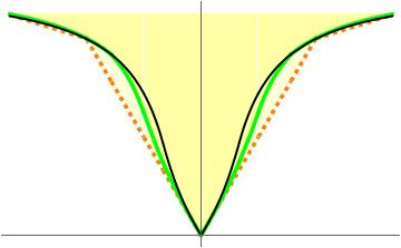
Figure 1. Joint spectrum of $(H_{\mathrm{Bog}},P)$ for generic potentials

One can perform an additional step in the Bogoliubov approach. If the potential $v$ has a very small support, one can argue that $\frac{\hat{v}({\mathbf{k}})}{\hat{v}(0)}$ can be approximated by $1$. One then usually says that the interaction is given by contact potentials, which are presented in the position representation as $v(x)=a\delta(x)$, where $a$ is a constant, called the scattering length. This, however, strictly speaking is not correct. The delta function needs a renormalization to become a well-defined interaction in the two-body case; in the $N$-body case the situation is even more problematic. Anyway, in this approximation, which is valid in the dilute case, we obtain a simpler dispersion relation

$$e_{\mathbf{k}}=\sqrt{\frac{1}{4}|{\mathbf{k}}|^{4}+\mu|{\mathbf{k}}|^{2}}.$$ (11)

On fig. 2 we show the energy-momentum spectrum corresponding to (11).

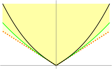
Figure 2. Joint spectrum of $(H_{\mathrm{Bog}},P)$ for contact potentials

The Hamiltonian $H_{\mathrm{Bog}}$, both with the dispersion relation (6) and (11) has remarkable physical consequences. Note first that the dispersion relation ${\mathbf{k}}\mapsto e_{\mathbf{k}}$ has a linear cusp at the bottom. It also has a positive critical velocity, that is,

$$c_{\mathrm{crit}}:=\sup\{c\ |\ e_{\mathbf{k}}\geq ck,\quad{\mathbf{k}}\in\mathrm{R}^{3}\}>0.$$ (12)

In other words, the graph ${\mathbf{k}}\mapsto e_{\mathbf{k}}$ is above ${\mathbf{k}}\mapsto c_{\mathrm{crit}}k$. The full joint spectrum $\sigma(P,H_{\mathrm{Bog}})$ is still above ${\mathbf{k}}\mapsto c_{\mathrm{crit}}k$. This is interpreted as one of the most important properties of superfluidity: a droplet of the Bose gas travelling with velocity less than $c_{\mathrm{crit}}k$ has negligible friction (see e.g. [11]).

Of course, $H_{\mathrm{Bog}}$ yields only an approximate description of the Bose gas. In reality, one cannot treat the quasiparticles given by $b_{\mathbf{k}}^{*},b_{\mathbf{k}}$ as fully independent. In the derivation of the Bogoliubov Hamiltonian various terms were neglected. In particular, terms of the third and fourth degree in $b_{\mathbf{k}}^{*},b_{\mathbf{k}}$ were dropped. Replacing $v$ by $\kappa v$ we obtain an (artificial) coupling constant, to be set to $1$ at the end. The third order terms are multiplied by $\sqrt{\kappa}$ and the quartic terms by $\kappa$. We argue that the quartic terms are of lower order and can be dropped. The third order terms have the form

$$\frac{1}{\sqrt{L^{3}}}\sum_{{\mathbf{k}},{\mathbf{p}},{\mathbf{k}}+{\mathbf{p}}\neq 0}u_{{\mathbf{k}},{\mathbf{p}}}b_{\mathbf{k}}^{*}b_{\mathbf{p}}^{*}b_{{\mathbf{k}}+{\mathbf{p}}}+\overline{u_{{\mathbf{k}},{\mathbf{p}}}}b_{{\mathbf{k}}+{\mathbf{p}}}b_{\mathbf{k}}^{*}b_{\mathbf{p}}^{*}$$ (13)

$$+ \frac{1}{\sqrt{L^{3}}}\sum_{{\mathbf{k}},{\mathbf{p}},{\mathbf{k}}+{\mathbf{p}}\neq 0}w_{{\mathbf{k}},{\mathbf{p}}}b_{\mathbf{k}}^{*}b_{\mathbf{p}}^{*}b_{-{\mathbf{k}}-{\mathbf{p}}}^{*}+\overline{w_{{\mathbf{k}},{\mathbf{p}}}}b_{-{\mathbf{k}}-{\mathbf{p}}}b_{\mathbf{k}}b_{\mathbf{p}}.$$ (14)

We will argue (see Section 6) that triple creation and triple annihilation terms do not contribute to the decay of phonons. Thus we drop also (14).

Let us investigate what happens with the quasiparticle state $b_{\mathbf{k}}^{*}\Omega_{\mathrm{Bog}}$ under the perturbation (13). The state $b_{\mathbf{k}}^{*}\Omega_{\mathrm{Bog}}$ couples only to the 2-quasiparticle sector. By taking thermodynamic limit we can assume that the variable ${\mathbf{k}}$ is continuous. Thus the perturbed quasiparticle can be described by the space $\mathbb{C}\oplus L^{2}(\mathbb{R}^{3})$ with the Hamiltonian

$$H_{\rm{Fried}}({\mathbf{k}}) :=\begin{bmatrix}e_{\mathbf{k}}&(h_{\mathbf{k}}|\\ |h_{\mathbf{k}})&e_{\mathbf{p}}+e_{{\mathbf{k}}-{\mathbf{p}}}\end{bmatrix},$$ (15)

and $h_{\mathbf{k}}$ can be derived from (13). Hamiltonians similar to this one are well understood. They are often used as toy models in quantum physics and are sometimes called Friedrichs Hamiltonians.

It is important to notice that, if we set $\hat{v}=0$, so that the off-diagonal terms in (15) disappear, the unperturbed quasiparticle energy $e_{\mathbf{k}}$ lies inside the continuous spectrum of 2-quasiparticle excitations $\{e_{\mathbf{p}}+e_{{\mathbf{k}}-{\mathbf{p}}}\ |\ {\mathbf{p}}\in\mathbb{R}^{3}\}$, at least for small momenta. (To be able to say this we need thermodynamic limit which makes the momentum continuous.) To see this, note that if ${\mathbf{k}}\mapsto e_{\mathbf{k}}$ is convex we have a particularly simple expression (cf. Lemma 1) for the infimum of the 2-quasiparticle spectrum:

$$\inf_{{\mathbf{p}}}\{e_{\mathbf{p}}+e_{{\mathbf{k}}-{\mathbf{p}}}\}=2e_{{\mathbf{k}}/2}.$$ (16)

Now (11) is strictly convex, hence $e_{\mathbf{k}}$ lies inside the continuous spectrum of 2-quasiparticle excitations. The generic dispersion relation (6) is convex for small momenta, hence this property is true at least for small momenta.

Because of that, one can expect that the position of the singularity of the resolvent of (15) becomes complex—it describes a resonance and not a bound state. This is interpreted as the unstability of the quasiparticle: its decay rate is twice the imaginary part of the resonance.

The second order perturbation theory, often called the Fermi Golden Rule, says that in order to compute the (complex) energy shift of an eigenvalue we need to find the so-called self-energy $\Sigma_{\mathbf{k}}(z)$, which for $z\not\in\mathbb{R}$ in our case is given by the integral

$$\Sigma_{\mathbf{k}}(z) =\frac{1}{(2\pi)^{3}}\int\frac{h_{\mathbf{k}}^{2}({\mathbf{p}})\,{\rm d}{\mathbf{p}}}{(z-e_{\mathbf{p}}-e_{{\mathbf{k}}-{\mathbf{p}}})}.$$ (17)

Then $\Sigma_{\mathbf{k}}(e_{\mathbf{k}}+\mathrm{i}0)$ should give the energy shift of the eigenvalue $e_{\mathbf{k}}$.

The imaginary part of this shift is much easier to compute. In fact, applying the Sochocki-Plemelj formula $\frac{1}{x+\mathrm{i}0}=\mathcal{P}\frac{1}{x}-\mathrm{i}\pi\delta(x)$ we obtain

$$\mathrm{Im}\Sigma_{\mathbf{k}}(e_{\mathbf{k}}+\mathrm{i}0) =\frac{1}{8\pi^{2}}\int h^{2}({\mathbf{p}})\delta(e_{\mathbf{k}}-e_{\mathbf{p}}-e_{{\mathbf{k}}-{\mathbf{p}}})\,{\rm d}{\mathbf{p}}.$$ (18)

In Theorem 2 we prove that if $e_{\mathbf{k}}$ is given by (11), then

$$\mathrm{Im}\Sigma_{{\mathbf{k}}}(e_{k}+\mathrm{i}0)=-c_{\mathrm{Bel}}k^{5}+O(k^{6})\qquad\text{as}\qquad k\to 0,\qquad c_{\mathrm{Bel}}=\frac{3\hat{v}(0)}{640\pi^{2}\mu}k^{5}.$$ (19)

In fact, our result could be also extended to the case of (6), but for the sake of clarity of the presentation we present the proof only for (11). Physically (19) means that quasiparticles are almost stable for small $k$ with the lifetime proportional to $k^{-5}$. (19) is the main result of our paper.

We remark that our analysis is based on the grand-canonical approach where $\mu$ is the chemical potential. One can go back to the canonical picture. To this end one determines the chemical potential as a function of the density. In the Bogoliubov approximation one obtains to leading order that $\rho\approx\mu/\hat{v}(0)$. Furthermore, also $\rho\approx\rho_{0}$, where $\rho_{0}$ is the condensate density, holds to leading order and thus the proportionality constant can be written as

$$c_{\mathrm{Bel}}=\frac{3}{640\pi^{2}\rho_{0}},$$ (20)

which is the form of this result which is usually stated in the physics literature ([36, 19, 28, 13]).

One could naively expect that the same method gives the correction to the real part of the dispersion relation. Unfortunately, $\mathrm{Re}\Sigma_{{\mathbf{k}}}(z)$ obtained from (17) is ill defined because of the divergence of the integral at large momenta. One can impose a cut-off and try to renormalize. For instance, one can replace $h_{\mathbf{k}}({\mathbf{p}})$ by

$$h_{\mathbf{k}}^{\Lambda}({\mathbf{p}}):=h_{\mathbf{k}}({\mathbf{p}})\theta(\Lambda-{\mathbf{p}}-|{\mathbf{k}}-{\mathbf{p}}|),$$ (21)

where $\theta$ is the Heaviside function. (Note that the details of the cutoff are not physically relevant; (21) is especially convenient for computations, because it respects the natural symmetry of the problem). The cut-off self-energy

$$\Sigma_{\mathbf{k}}^{\Lambda}(z) =\frac{1}{(2\pi)^{3}}\int\frac{(h_{\bf k}^{\Lambda}({\mathbf{p}}))^{2}\,{\rm d}{\mathbf{p}}}{(z-e_{\mathbf{p}}-e_{{\mathbf{k}}-{\mathbf{p}}})}$$ (22)

is well defined.

Let us now try to remove the dependence of the self-energy on the cutoff. The most satisfactory renormalization scenario would be to find a counterterm $c^{\Lambda}$ independent of ${\mathbf{k}}$ so that

$$\lim_{\Lambda\to\infty}\big{(}\Sigma_{\mathbf{k}}^{\Lambda}(z)-c^{\Lambda}\big{)}\quad\text{ exists. }$$ (23)

An initial positive result suggests that one can hope for a removal of the ultraviolet cutoff in the self-energy: there exists the limit

$$\lim_{\Lambda\to\infty}\big{(}\Sigma_{\mathbf{k}}^{\Lambda}(z)-\Sigma_{\mathbf{k}}^{\Lambda}(0)\big{)}.$$ (24)

Unfortunately, $\lim\limits_{{\mathbf{k}}\to 0}\Sigma_{\mathbf{k}}^{\Lambda}(0)=\infty$, which implies that finding a $c^{\Lambda}$ such that (23) is true is impossible. This is the content of Theorem 3. Thus the physical meaning of the quantity (24) is dubious, because the counterterm $\Sigma_{\mathbf{k}}^{\Lambda}(0)$ depends on the momentum ${\mathbf{k}}$. We leave the interpretation of this result open.

One can conclude that perturbation theory around the Bogoliubov Hamiltonian provides a reasonable method to find the second order imaginary correction to the dispersion relation. However, by this method we seem not able to compute its real part. This is not very surprising. It is a general property of Friedrichs Hamiltonians with singular off-diagonal terms: the imaginary part of the perturbed eigenvalue can be computed much more reliably than its real part. We describe this briefly in Sections 2 and 3.

The above problem is an indication of the crudeness of the Bogoliubov approximation. Throwing out the zero mode from the picture (or, which is essentially the same, treating it as a classical quantity), as well as throwing out higher order terms, is a very violent act and we should not be surprised by a punishment. By the way, one expects that the true dispersion relation of phonons goes to zero as ${\mathbf{k}}\to 0$. This is the content of the so called “Hugenholtz-Pines Theorem” [24], which is a (non-rigorous) argument based on the gauge invariance. Perturbation theory around the Bogoliubov Hamiltonian is compatible with this theorem where it comes to the imaginary part. For the real part it fails.

Let us now make a few remarks about the literature. The orginal paper of Bogoliubov [5] was heuristic, however in recent years there have been many rigorous papers justifying Bogoliubov’s approximation in several cases. The first result justifying (7) has been obtained in the mean-field scaling by Seiringer in [35] (see also [26, 17, 20, 32] for related results). Recently, corresponding results have been obtained in the Gross-Pitaevskii regime [3, 10, 33] and even beyond [9]. A time-dependent version of Bogoliubov theory has been successful in describing the dynamics of Bose-Einstein condensates and excitations thereof (see [30, 34] for reviews).

As explained above, to describe damping one has to go beyond Bogoliubov theory. In the mean-field regime this has been done for the ground state energy expansion in [31, 8] and for the dynamics in [7]. Very recently, the extension of [8] to singular interactions has been obtained in [6].

None of the above rigorous papers, with exception of [17], addressed the energy-momentum spectrum. In fact, it is very difficult to study rigorously the dispersion relation in thermodynamic limit—which is essentially necessary to analyze phonon damping.

The quasiparticle picture of the Bose gas at low temperatures has been confirmed in experiments. The dispersion relation of ${}^{4}\mathrm{He}$ can be observed in neutron scattering experiments, and is remarkably sharp. It has been measured within a large range of wave numbers covering not only phonons, but also the so-called maxons and rotons, see e.g. [21]. In particular, one can see that the dispersion relation is slightly higher than the 2-quasiparticle spectrum for low wave numbers. The quasiparticle picture has also been confirmed by experiments on Bose Einstein condensates involving alkali atoms. The Beliaev damping has been observed in experiments on Bose Einstein condensates. The results are consistent with theoretical predictions [25, 22]. Note, however, that the precise prediction (18) is difficult to verify experimentally. Bose-Einstein condensates created in labs are not very large, so it is difficult to probe the large wavelength region.

Let us mention that there exists another phenomenon found in Bose-Einstein condensates, the so-called Landau damping, which involves instability of quasiparticles due to thermal excitations. The Landau damping is absent at zero temperature and becomes dominant at higher temperatures. The Beliaev damping occurs at zero temperature, and for very small temperatures it is still stronger than the Landau damping.

In the physics literature, the damping of phonons was first computed by Beliaev [2]. Lanadu damping has been for the first time computed by Hohenberg and Martin in [23] (see also [29]). Both these results have been reproduced in [36], also using the formalism of Feynman diagrams and many-body Green’s functions. In [28] the damping rate was derived starting from an effective action in the spirit of Popov’s hydrodynamical approach. [19] repeated the same computation in the time-dependent mean-field approach. In [13] the mean-field and hydrodynamic approaches were applied to the 2D case. Our derivation is consistent with the above works, however, in our opinion, avoids some unnecessary elements obscuring the simple mechanism of the Beliaev damping.

The plan of the paper is as follows. Sections 2 and 3 concern general well-known facts about about 2nd order perturbation theory of embedded eigenvalues. In Section 4 we define the Bose gas Hamiltonian and describe the Bogoliubov approach in the grand-canonical setting. In Section 5 we derive heuristically the effective model that we consider. Then, in Section 6 we discuss the shape of the energy-momentum spectrum and explain why the contribution from term (14) is irrelevant for the damping rate computation, which is the main result of the paper is proven in Section 8 as Theorem 2. The analysis why computing the real part of the self-energy fails by the method of this paper is described in Section 9.

Acknowledgements. The work of all authors was supported by the Polish-German NCN-DFG grant Beethoven Classic 3 (project no. 2018/31/G/ST1/01166).

2. Friedrichs Hamiltonian

Suppose that $\mathcal{H}$ is a Hilbert space with a self-adjoint operator $H$. Let $\Psi\in\mathcal{H}$ be a normalized vector. We can write $\mathcal{H}\simeq\mathbb{C}\oplus\mathcal{K}$, where $\mathbb{C}\simeq\mathbb{C}\Psi$ and $\mathcal{K}:=\{\Psi\}^{\perp}$. First assume that $\Psi$ belongs to the domain of $H$ and set

$$h:=H\Psi,\quad E_{0}:=(\Psi|H\Psi).$$ (25)

Let $K$ denote $H$ compressed to $\mathcal{K}$. That means, if $I:\mathcal{K}\to\mathcal{H}$ is the embedding, then $K:=I^{*}HI$. Then in terms of $\mathbb{C}\oplus\mathcal{K}$ we can write

$$H=\begin{bmatrix}E_{0}&(h|\\ |h)&K\end{bmatrix}.$$ (26)

Operators of this form were studied by Friedrichs in [18]. Therefore, sometimes they are referred to as Friedrichs Hamiltonians.

Let $z\in\mathbb{C}$. The following identity is a special case of the so-called Feshbach-Schur formula:

$$(\Psi|(H-z)^{-1}\Psi) =\frac{1}{E_{0}+\Sigma(z)-z},$$ (27)

$$\Sigma(z) =-(h|(K-z)^{-1}h).$$ (28)

Following a part of the physics literature, we will call $\Sigma(z)$ the self-energy. For further reference let us rewrite (27) as

$$\Sigma(z)=\frac{1}{(\Psi|(H-z)^{-1}\Psi)}+z-E_{0},$$ (29)

and let us describe the full resolvent:

$$(H-z)^{-1}= \begin{bmatrix}0&0\\ 0&(K-z)^{-1}\end{bmatrix}$$ (30)

$$+ \begin{bmatrix}1\\ (K-z)^{-1}|h)\end{bmatrix}\frac{1}{E_{0}+\Sigma(z)-z}\begin{bmatrix}1&(h|(K-z)^{-1}\end{bmatrix}.$$

We can apply the above formulas also if $\Psi$ does not belong to the domain of $H$, but belongs to its form domain, so that $(\Psi|H\Psi)$ is well defined. Note that $E_{0}$ and $\Sigma(z)$ are then uniquely defined by (25) and (29)).

If $\Psi$ does not belong to the form domain of $H$, then strictly speaking the self-energy is ill defined. In practice in such situations one often introduces a cutoff Hamiltonian $H^{\Lambda}$, which in some sense approximates $H$. Then, setting $h^{\Lambda}:=H^{\Lambda}\Psi$, $E_{0}^{\Lambda}:=(\Psi|H^{\Lambda}\Psi)$, and denoting by $K^{\Lambda}$ the operator $H^{\Lambda}$ compressed to $\mathcal{K}$, one can use the cutoff version of the Feshbach-Schur formula:

$$(\Psi|(H^{\Lambda}-z)^{-1}\Psi) =\frac{1}{E_{0}^{\Lambda}+\Sigma^{\Lambda}(z)-z},$$ (31)

$$\Sigma^{\Lambda}(z) =-(h^{\Lambda}|(K^{\Lambda}-z)^{-1}h^{\Lambda}).$$ (32)

The resolvent of the original Hamiltonian $H$ can be retrieved [16] in the limit $\Lambda\to\infty$:

$$(H-z)^{-1}=\lim_{\Lambda\to\infty}(H^{\Lambda}-z)^{-1}.$$ (33)

Note that $E_{0}^{\Lambda}$ is a sequence of real numbers, typically converging to $\infty$. They can be treated as counterterms renormalizing the self-energy $\Sigma^{\Lambda}(z)$.

3. Fermi Golden Rule

The meaning of the self-energy is especially clear in perturbation theory. Again, let $\Psi$ be a normalized vector in $\mathcal{H}$. Consider a family of self-adjoint operators $H_{\lambda}=H_{0}+\lambda V$ such that $H_{0}\Psi=E_{0}\Psi$ and $(\Psi|V\Psi)=0$. Let $h:=V\Psi$ and $K_{\lambda}$ be $H_{\lambda}$ compressed to $\mathcal{K}$. Thus we can rewrite (26) as

$$H_{\lambda}=\begin{bmatrix}E_{0}&\lambda(h|\\ \lambda|h)&K_{\lambda}\end{bmatrix}.$$ (34)

We extract $\lambda^{2}$ from the definition of the self-energy, so that (27) and (28) are rewritten as

$$(\Psi|(H_{\lambda}-z)^{-1}\Psi) =\big{(}E_{0}+\lambda^{2}\Sigma_{\lambda}(z)-z\big{)}^{-1},$$ (35)

$$\Sigma_{\lambda}(z) :=-(h|(K_{\lambda}-z)^{-1}h)=\Sigma_{0}(z)+O(\lambda).$$ (36)

Now (35) has a pole at

$$E_{0}+\lambda^{2}\Sigma_{0}(E_{0}+\mathrm{i}0)+O(\lambda^{3}).$$ (37)

This is often formulated as the Fermi Golden Rule: the pole of the resolvent, originally at an eigenvalue $E_{0}$, is shifted in the second order by $\lambda^{2}\Sigma_{0}(E_{0}+\mathrm{i}0)$. This shift can have a negative imaginary part, and then the eigenvalue disappears. A singularity of the resolvent with a negative imaginary part is usually called a resonance.

Resonances describe metastable states. A rigorous meaning of a resonance is provided by the following version of the weak coupling limit ([12], see also [14, 15])

$$\lim_{\lambda\to 0}\big{(}\Psi\big{|}\exp\big{(}-\mathrm{i}\tfrac{t}{\lambda^{2}}(H_{\lambda}-E_{0})\big{)}\big{|}\Psi\big{)}=\mathrm{e}^{-\mathrm{i}t\Sigma_{0}(E_{0}+i0)}.$$ (38)

If the perturbation is singular, so that $\Psi$ does not belong to the domain of $V$, then $\Sigma_{0}(z)$ is in general ill defined and (37) may lose its meaning. Strictly speaking, one then needs to introduce a cutoff on the perturbation and a counterterm, and only then to apply the appropriately modified Fermi Golden Rule.

Note that it is enough to consider real counterterms. Therefore, if we know that the renormalized energy is close to $E_{0}$, then we can still expect that (37) gives a correct prediction for the imaginary part of the resonance. In other words, the imaginary part of the singularity of the resolvent $(H_{\lambda}-z)^{-1}$ is

$$\lambda^{2}\mathrm{Im}\Sigma_{0}(E_{0}+\mathrm{i}0)+O(\lambda^{3}),$$ (39)

where we do not need to cut off the perturbation.

In practice, we start from a singular expression of the form 34. To make it well-defined we need to choose a cutoff and counterterms. These choices will not affect the imaginary part of the resonance, however in principle, one can add an arbitrary real constant to a counterterm, which will affect the real part of the resonance. Therefore, for singular perturbations it may be more difficult to predict the real part of the resonance.

4. Bose gas and Bogoliubov ansatz

We consider a homogeneous Bose gas of $N$ particles with a two-body potential described by a function $v:\mathbb{R}^{3}\to\mathbb{R}$ whose Fourier transform $\hat{v}({\mathbf{k}})=\int_{\mathbb{R}^{3}}v(x)\mathrm{e}^{-\mathrm{i}{\mathbf{k}}\cdot{\mathbf{x}}}\,{\rm d}{\mathbf{x}}$ is non-negative and rotation invariant. In the grand canonical setting and the momentum representation such a system is governed by the (second quantized) Hamiltonian

$$H=\int\left(\frac{{\mathbf{k}}^{2}}{2}-\mu\right)a_{\mathbf{k}}^{*}a_{\mathbf{k}}\,{\rm d}{\mathbf{k}}+\frac{\kappa}{2(2\pi)^{3}}\int\,{\rm d}{\mathbf{p}}\int\,{\rm d}{\mathbf{q}}\int\,{\rm d}{\mathbf{k}}\hat{v}({\mathbf{k}})a_{{\mathbf{p}}-{\mathbf{k}}}^{*}a_{{\mathbf{q}}+{\mathbf{k}}}^{*}a_{{\mathbf{p}}}a_{{\mathbf{q}}},$$ (40)

where $\mu\geq 0$ is the chemical potential and $a_{\mathbf{k}}^{*}/a_{\mathbf{k}}$ the creation/annihilation operators for particles of mode ${\mathbf{k}}$. It acts on the bosonic Fock space $\mathcal{F}=\Gamma_{\mathrm{s}}\big{(}L^{2}(\mathbb{R}^{3})\big{)}$, and for each $N$ it leaves invariant its $N$-particle sector $L^{2}_{\mathrm{s}}\big{(}(\mathbb{R}^{3})^{N}\big{)}$. Recall that the creation and annihilation operators satisfy the canonical commutation relation (CCR):

$$[a_{\mathbf{p}},a_{\mathbf{q}}]=0=[a_{\mathbf{p}}^{*},a_{\mathbf{q}}^{*}],\ \ [a_{\mathbf{p}},a^{*}_{\mathbf{q}}]=\delta({\mathbf{p}}-{\mathbf{q}}),$$ (41)

where $[\ ,\ ]$ is the usual commutator. We introduce the coupling constant $\kappa>0$ mostly for bookkeeping purposes; note that in the introduction we set $\kappa=1$.

For the reasons explained in the introduction, we replace the infinite space $\mathbb{R}^{3}$ by the torus $[-L/2,L/2]^{3}$ with periodic boundary conditions. In the momentum representation the Hamiltonian becomes

$$H=\sum_{{\mathbf{k}}\in 2\pi\mathbb{Z}^{3}/L}\left(\frac{{\mathbf{k}}^{2}}{2}-\mu\right)a_{\mathbf{k}}^{*}a_{\mathbf{k}}+\frac{\kappa}{2L^{3}}\sum_{{\mathbf{p}},{\mathbf{q}},{\mathbf{k}}\in 2\pi\mathbb{Z}^{3}/L}\hat{v}({\mathbf{k}})a_{{\mathbf{p}}-{\mathbf{k}}}^{*}a_{{\mathbf{q}}+{\mathbf{k}}}^{*}a_{{\mathbf{p}}}a_{{\mathbf{q}}}.$$ (42)

Note that $\hat{v}$ is the same function as in (40), however it is now sampled only on the lattice $2\pi\mathbb{Z}^{3}/L$. The commutation relation involve now the Kronecker delta:

$$[a_{\mathbf{p}},a_{\mathbf{q}}]=0=[a_{\mathbf{p}}^{*},a_{\mathbf{q}}^{*}],\ \ [a_{\mathbf{p}},a^{*}_{\mathbf{q}}]=\delta_{{\mathbf{p}},{\mathbf{q}}}.$$ (43)

Let us now pass to the quasiparticle representation. To this end we follow the well-known grand-canonical version of the Bogoliubov approach (see e.g. [11]). It involves two unitary transformations.

The first one is a Weyl transformation that introduces a macroscopic occupation of the zero-momentum mode, the Bose-Einstein condensate. (In the canonical version Bogoliubov approach this corresponds to the c-number substitution [27].) To this end, for $\alpha\in\mathbb{C}$, we introduce the Weyl operator of the mode ${\mathbf{k}}=0$

$$W_{\alpha}=\exp(-\alpha a_{0}^{*}+\bar{\alpha}a_{0}).$$ (44)

Then

$$W_{\alpha}^{*}a^{*}_{\mathbf{k}}W_{\alpha}=a^{*}_{\mathbf{k}}-\bar{\alpha}\delta_{{\mathbf{k}},0}=:\tilde{a}^{*}_{{\mathbf{k}}}.$$

The new annihilation operators with tildes kill the “new vacuum” $\Omega_{\alpha}=W^{*}_{\alpha}\Omega$. We express our Hamiltonian in terms of $\tilde{a}_{\mathbf{k}}^{*},\tilde{a}_{\mathbf{k}}$. To simplify the notation, in what follows we drop the tildes and we obtain

$$H = -\mu|\alpha|^{2}+\frac{\kappa\hat{v}(0)}{2L^{3}}|\alpha|^{4}+\left(\frac{\kappa\hat{v}(0)}{L^{3}}|\alpha|^{2}-\mu\right)(\alpha a_{0}^{*}+\bar{\alpha}a_{0})$$

$$+ \sum_{{\mathbf{k}}}\left(\frac{{\mathbf{k}}^{2}}{2}-\mu+\frac{\kappa(\hat{v}({\mathbf{k}})+\hat{v}(0))}{L^{3}}|\alpha|^{2}\right)a_{\mathbf{k}}^{*}a_{\mathbf{k}}+\sum_{{\mathbf{k}}}\frac{\kappa\hat{v}({\mathbf{k}})}{2L^{3}}\left(\alpha^{2}a_{\mathbf{k}}^{*}a_{-{\mathbf{k}}}^{*}+\bar{\alpha}^{2}a_{\mathbf{k}}a_{-{\mathbf{k}}}\right)$$

$$+ \frac{\kappa}{L^{3}}\sum_{{\mathbf{k}}_{1},{\mathbf{k}}_{2}}\hat{v}({\mathbf{k}}_{1})\left(\bar{\alpha}a_{{\mathbf{k}}_{1}+{\mathbf{k}}_{2}}^{*}a_{{\mathbf{k}}_{1}}a_{{\mathbf{k}}_{2}}+\alpha a_{{\mathbf{k}}_{1}}^{*}a_{{\mathbf{k}}_{2}}^{*}a_{{\mathbf{k}}_{1}+{\mathbf{k}}_{2}}\right)$$

$$+ \frac{\kappa}{2L^{3}}\sum_{{\mathbf{k}}_{1},{\mathbf{k}}_{2},{\mathbf{k}}_{3},{\mathbf{k}}_{4}}\delta({\mathbf{k}}_{1}+{\mathbf{k}}_{2}-{\mathbf{k}}_{3}-{\mathbf{k}}_{4})\hat{v}({\mathbf{k}}_{2}-{\mathbf{k}}_{3})a_{{\mathbf{k}}_{1}}^{*}a_{{\mathbf{k}}_{2}}^{*}a_{{\mathbf{k}}_{3}}a_{{\mathbf{k}}_{4}}.$$

Note that we have

$$(\Omega_{\alpha}|H\Omega_{\alpha})=-\mu|\alpha|^{2}+\frac{\kappa\hat{v}(0)}{2L^{3}}|\alpha|^{4},$$

and we choose $\alpha=\sqrt{\frac{\mu L^{3}}{\kappa\hat{v}(0)}}$, so that $\Omega_{\alpha}$ minimizes this expectation value. This leads to

$$H =\kappa^{-1}H_{0}+H_{2}+\sqrt{\kappa}H_{3}+\kappa H_{4},$$ (45)

$$H_{0} :=-\frac{\mu^{2}L^{3}}{2\hat{v}(0)},$$

$$H_{2} :=\sum_{{\mathbf{k}}}\left(\frac{{\mathbf{k}}^{2}}{2}+\frac{\mu\hat{v}({\mathbf{k}})}{\hat{v}(0)}\right)a_{\mathbf{k}}^{*}a_{\mathbf{k}}+\sum_{{\mathbf{k}}}\frac{\mu\hat{v}({\mathbf{k}})}{2\hat{v}(0)}\left(a_{\mathbf{k}}^{*}a_{-{\mathbf{k}}}^{*}+a_{\mathbf{k}}a_{-{\mathbf{k}}}\right),$$

$$H_{3} :=\frac{1}{L^{3/2}}\sum_{{\mathbf{k}}_{1},{\mathbf{k}}_{2}}\frac{\hat{v}({\mathbf{k}}_{1})\sqrt{\mu}}{\sqrt{\hat{v}(0)}}\left(a_{{\mathbf{k}}_{1}+{\mathbf{k}}_{2}}^{*}a_{{\mathbf{k}}_{1}}a_{{\mathbf{k}}_{2}}+a_{{\mathbf{k}}_{1}}^{*}a_{{\mathbf{k}}_{2}}^{*}a_{{\mathbf{k}}_{1}+{\mathbf{k}}_{2}}\right),$$

$$H_{4} :=\frac{1}{2L^{3}}\sum_{{\mathbf{k}}_{1},{\mathbf{k}}_{2},{\mathbf{k}}_{3},{\mathbf{k}}_{4}}\delta({\mathbf{k}}_{1}+{\mathbf{k}}_{2}-{\mathbf{k}}_{3}-{\mathbf{k}}_{4})\hat{v}({\mathbf{k}}_{2}-{\mathbf{k}}_{3})a_{{\mathbf{k}}_{1}}^{*}a_{{\mathbf{k}}_{2}}^{*}a_{{\mathbf{k}}_{3}}a_{{\mathbf{k}}_{4}}.$$

We extract from the above Hamiltonian all terms containing only non-zero modes:

$$H_{2} =\frac{\mu}{2}(a_{0}^{*2}+a_{0}^{2}+2a_{0}^{*}a_{0})+H_{2}^{\rm exc},$$

$$H_{2}^{\rm exc} :=\sum_{{\mathbf{k}}\neq 0}\left(\frac{{\mathbf{k}}^{2}}{2}+\frac{\mu\hat{v}({\mathbf{k}})}{\hat{v}(0)}\right)a_{\mathbf{k}}^{*}a_{\mathbf{k}}+\sum_{{\mathbf{k}}\neq 0}\frac{\mu\hat{v}({\mathbf{k}})}{2\hat{v}(0)}\left(a_{\mathbf{k}}^{*}a_{-{\mathbf{k}}}^{*}+a_{\mathbf{k}}a_{-{\mathbf{k}}}\right);$$ (46)

$$H_{3} =\frac{1}{L^{3/2}}\sum_{{\mathbf{k}}}\sqrt{\mu\hat{v}(0)}(a_{0}^{*}+a_{0})a_{\mathbf{k}}^{*}a_{\mathbf{k}}$$

$$+\frac{1}{L^{3/2}}\sum_{{\mathbf{k}}\neq 0}\frac{\sqrt{\mu}\hat{v}({\mathbf{k}})}{\sqrt{\hat{v}(0)}}\big{(}(a_{0}^{*}+a_{0})a_{\mathbf{k}}^{*}a_{\mathbf{k}}+a_{0}a_{\mathbf{k}}^{*}a_{-{\mathbf{k}}}^{*}+a_{0}^{*}a_{\mathbf{k}}a_{-{\mathbf{k}}}\big{)}+H_{3}^{\rm exc},$$

$$H_{3}^{\rm exc} :=\frac{1}{L^{3/2}}\sum_{{\mathbf{k}}_{1},{\mathbf{k}}_{2},{\mathbf{k}}_{1}+{\mathbf{k}}_{2}\neq 0}\frac{\hat{v}({\mathbf{k}}_{1})\sqrt{\mu}}{\sqrt{\hat{v}(0)}}\left(a_{{\mathbf{k}}_{1}+{\mathbf{k}}_{2}}^{*}a_{{\mathbf{k}}_{1}}a_{{\mathbf{k}}_{2}}+a_{{\mathbf{k}}_{1}}^{*}a_{{\mathbf{k}}_{2}}^{*}a_{{\mathbf{k}}_{1}+{\mathbf{k}}_{2}}\right);$$ (47)

$$H_{4} =\frac{1}{2L^{3}}\hat{v}(0)\Big{(}a_{0}^{*}a_{0}^{*}a_{0}a_{0}+2\sum_{{\mathbf{k}}\neq 0}a_{0}^{*}a_{0}a_{\mathbf{k}}^{*}a_{\mathbf{k}}\Big{)}$$

$$+\frac{1}{2L^{3}}\sum_{{\mathbf{k}}\neq 0}\hat{v}({\mathbf{k}})(a_{0}^{*}a_{0}^{*}a_{\mathbf{k}}a_{-{\mathbf{k}}}+a_{0}a_{0}a_{\mathbf{k}}^{*}a_{-{\mathbf{k}}}^{*}+2a_{0}^{*}a_{0}a_{\mathbf{k}}^{*}a_{\mathbf{k}})$$

$$+\frac{1}{L^{3}}\sum_{{\mathbf{k}}_{1},{\mathbf{k}}_{2},{\mathbf{k}}_{1}+{\mathbf{k}}_{2}\neq 0}\hat{v}(k_{1})\big{(}a_{0}^{*}a_{{\mathbf{k}}_{1}+{\mathbf{k}}_{2}}^{*}a_{{\mathbf{k}}_{1}}a_{{\mathbf{k}}_{2}}+a_{0}a_{{\mathbf{k}}_{1}}^{*}a_{{\mathbf{k}}_{2}}^{*}a_{{\mathbf{k}}_{1}+{\mathbf{k}}_{2}}\big{)}+H_{4}^{\rm exc},$$

$$H_{4}^{\rm exc} :=\frac{1}{2L^{3}}\sum_{{\mathbf{k}}_{1},{\mathbf{k}}_{2},{\mathbf{k}}_{3},{\mathbf{k}}_{4}\neq 0}\delta({\mathbf{k}}_{1}+{\mathbf{k}}_{2}-{\mathbf{k}}_{3}-{\mathbf{k}}_{4})\hat{v}({\mathbf{k}}_{2}-{\mathbf{k}}_{3})a_{{\mathbf{k}}_{1}}^{*}a_{{\mathbf{k}}_{2}}^{*}a_{{\mathbf{k}}_{3}}a_{{\mathbf{k}}_{4}}.$$ (48)

We are going to apply a Bogoliubov transformation

$$U_{\mathrm{Bog}}:=\exp\Bigg{(}\sum_{{\mathbf{k}}\neq 0}\beta_{\mathbf{k}}(a_{\mathbf{k}}^{*}a_{-{\mathbf{k}}}^{*}-a_{\mathbf{k}}a_{-{\mathbf{k}}})\Bigg{)},$$ (49)

which transforms non-zero mode operators $a_{\mathbf{k}}^{*},a_{\mathbf{k}}$ into quasi-particle operators $b_{\mathbf{k}}^{*},b_{\mathbf{k}}$:

$$b_{\mathbf{k}} := U_{\mathrm{Bog}}a_{\mathbf{k}}U_{\mathrm{Bog}}^{*}=\sigma_{\mathbf{k}}a_{\mathbf{k}}+\gamma_{\mathbf{k}}a_{-{\mathbf{k}}}^{*},$$

$$b_{\mathbf{k}}^{*} := U_{\mathrm{Bog}}a_{\mathbf{k}}^{*}U_{\mathrm{Bog}}^{*}=\sigma_{\mathbf{k}}a_{\mathbf{k}}^{*}+\gamma_{\mathbf{k}}a_{-{\mathbf{k}}},$$ (50)

where

$$\sigma_{\mathbf{k}} =\frac{\sqrt{\sqrt{e_{\mathbf{k}}^{2}+B_{\mathbf{k}}^{2}}+e_{\mathbf{k}}}}{\sqrt{2e_{\mathbf{k}}}},\quad\gamma_{\mathbf{k}}=\frac{\sqrt{\sqrt{e_{\mathbf{k}}^{2}+B_{\mathbf{k}}^{2}}-e_{\mathbf{k}}}}{\sqrt{2e_{\mathbf{k}}}},$$

$$e_{\mathbf{k}} :=\sqrt{\frac{1}{4}|{\mathbf{k}}|^{4}+B_{\mathbf{k}}|{\mathbf{k}}|^{2}},\ \ \ B_{\mathbf{k}}:=\frac{\hat{v}({\mathbf{k}})}{\hat{v}(0)}\mu.$$

The inverse relation is

$$a_{\mathbf{k}} = \sigma_{\mathbf{k}}b_{\mathbf{k}}-\gamma_{\mathbf{k}}b_{-{\mathbf{k}}}^{*},$$

$$a_{\mathbf{k}}^{*} = \sigma_{\mathbf{k}}b_{\mathbf{k}}^{*}-\gamma_{\mathbf{k}}b_{-{\mathbf{k}}}.$$

It is well known that (50) diagonalizes $H_{2}^{\rm exc}$ in terms of the quasi-particle operators:

$$H_{2}^{{\rm exc}} = E_{\rm Bog}+H_{\mathrm{Bog}},$$ (51)

where

$$E_{\rm Bog} :=-\frac{1}{2}\sum_{{\mathbf{k}}\neq 0}\left(\frac{1}{2}|{\mathbf{k}}|^{2}+\frac{\hat{v}({\mathbf{k}})}{\hat{v}(0)}\mu-e_{\mathbf{k}}\right),$$ (52)

$$\qquad H_{\mathrm{Bog}} :=\sum_{{\mathbf{k}}\neq 0}e_{\mathbf{k}}b_{\mathbf{k}}^{*}b_{\mathbf{k}}.$$ (53)

We also express $H_{3}^{\rm exc}$ in terms of quasiparticles:

$$H_{3}^{\rm exc} =\frac{1}{L^{3/2}}\sum_{{\mathbf{k}}_{1},{\mathbf{k}}_{2},{\mathbf{k}}_{1}+{\mathbf{k}}_{2}\neq 0}\frac{\sqrt{\mu}\hat{v}({\mathbf{k}}_{1})}{\sqrt{\hat{v}(0)}}(A({\mathbf{k}}_{1},{\mathbf{k}}_{2})+A^{*}({\mathbf{k}}_{1},{\mathbf{k}}_{2}),$$

$$A({\mathbf{k}}_{1},{\mathbf{k}}_{2})= \quad\sigma_{{\mathbf{k}}_{1}}\sigma_{{\mathbf{k}}_{2}}\sigma_{{\mathbf{k}}_{1}+{\mathbf{k}}_{2}}b_{{\mathbf{k}}_{1}}^{*}b_{{\mathbf{k}}_{2}}^{*}b_{{\mathbf{k}}_{1}+{\mathbf{k}}_{2}}-\gamma_{{\mathbf{k}}_{1}}\sigma_{{\mathbf{k}}_{2}}\sigma_{{\mathbf{k}}_{1}+{\mathbf{k}}_{2}}b_{{\mathbf{k}}_{2}}^{*}b_{-{\mathbf{k}}_{1}}b_{{\mathbf{k}}_{1}+{\mathbf{k}}_{2}}$$

$$-\gamma_{{\mathbf{k}}_{1}}\gamma_{{\mathbf{k}}_{2}}\sigma_{{\mathbf{k}}_{1}+{\mathbf{k}}_{2}}b_{{\mathbf{k}}_{1}}^{*}b_{-{\mathbf{k}}_{2}}b_{{\mathbf{k}}_{1}+{\mathbf{k}}_{2}}+\gamma_{{\mathbf{k}}_{1}}\gamma_{{\mathbf{k}}_{2}}\sigma_{{\mathbf{k}}_{1}+{\mathbf{k}}_{2}}b_{-{\mathbf{k}}_{1}}b_{-{\mathbf{k}}_{2}}b_{{\mathbf{k}}_{1}+{\mathbf{k}}_{2}}$$

$$-\sigma_{{\mathbf{k}}_{1}}\sigma_{{\mathbf{k}}_{2}}\gamma_{{\mathbf{k}}_{1}+{\mathbf{k}}_{2}}b_{{\mathbf{k}}_{1}}^{*}b_{{\mathbf{k}}_{2}}^{*}b_{-{\mathbf{k}}_{1}-{\mathbf{k}}_{2}}^{*}-\gamma_{{\mathbf{k}}_{1}}\sigma_{{\mathbf{k}}_{2}}\gamma_{{\mathbf{k}}_{1}+{\mathbf{k}}_{2}}b_{{\mathbf{k}}_{2}}^{*}b_{-{\mathbf{k}}_{1}-{\mathbf{k}}_{2}}^{*}b_{-{\mathbf{k}}_{1}}$$

$$+\sigma_{{\mathbf{k}}_{1}}\gamma_{{\mathbf{k}}_{2}}\gamma_{{\mathbf{k}}_{1}+{\mathbf{k}}_{2}}b_{{\mathbf{k}}_{1}}^{*}b_{-{\mathbf{k}}_{1}-{\mathbf{k}}_{2}}^{*}b_{-{\mathbf{k}}_{2}}-\gamma_{{\mathbf{k}}_{1}}\gamma_{{\mathbf{k}}_{2}}\gamma_{{\mathbf{k}}_{1}+{\mathbf{k}}_{2}}b_{-{\mathbf{k}}_{1}-{\mathbf{k}}_{2}}^{*}b_{-{\mathbf{k}}_{1}}b_{-{\mathbf{k}}_{2}}.$$

Thus

$$H_{3}^{\rm exc} =H_{3,1}^{\rm exc}+H_{3,2}^{\rm exc},$$ (54)

$$H_{3,1}^{\rm exc}=\sum_{{\mathbf{k}}_{1},{\mathbf{k}}_{2},{\mathbf{k}}_{1}+{\mathbf{k}}_{2}\neq 0}\frac{\sqrt{\mu}\hat{v}({\mathbf{k}}_{1})}{L^{3/2}\sqrt{\hat{v}(0)}} \Big{(}\sigma_{{\mathbf{k}}_{1}}\sigma_{{\mathbf{k}}_{2}}\sigma_{{\mathbf{k}}_{1}+{\mathbf{k}}_{2}}b_{{\mathbf{k}}_{1}}^{*}b_{{\mathbf{k}}_{2}}^{*}b_{{\mathbf{k}}_{1}+{\mathbf{k}}_{2}}-\gamma_{{\mathbf{k}}_{1}}\sigma_{{\mathbf{k}}_{2}}\sigma_{{\mathbf{k}}_{1}+{\mathbf{k}}_{2}}b_{{\mathbf{k}}_{2}}^{*}b_{-{\mathbf{k}}_{1}}b_{{\mathbf{k}}_{1}+{\mathbf{k}}_{2}}$$

$$- \gamma_{{\mathbf{k}}_{1}}\gamma_{{\mathbf{k}}_{2}}\sigma_{{\mathbf{k}}_{1}+{\mathbf{k}}_{2}}b_{{\mathbf{k}}_{1}}^{*}b_{-{\mathbf{k}}_{2}}b_{{\mathbf{k}}_{1}+{\mathbf{k}}_{2}}-\gamma_{{\mathbf{k}}_{1}}\sigma_{{\mathbf{k}}_{2}}\gamma_{{\mathbf{k}}_{1}+{\mathbf{k}}_{2}}b_{{\mathbf{k}}_{2}}^{*}b_{-{\mathbf{k}}_{1}-{\mathbf{k}}_{2}}^{*}b_{-{\mathbf{k}}_{1}}$$

$$+ \sigma_{{\mathbf{k}}_{1}}\gamma_{{\mathbf{k}}_{2}}\gamma_{{\mathbf{k}}_{1}+{\mathbf{k}}_{2}}b_{{\mathbf{k}}_{1}}^{*}b_{-{\mathbf{k}}_{1}-{\mathbf{k}}_{2}}^{*}b_{-{\mathbf{k}}_{2}}-\gamma_{{\mathbf{k}}_{1}}\gamma_{{\mathbf{k}}_{2}}\gamma_{{\mathbf{k}}_{1}+{\mathbf{k}}_{2}}b_{-{\mathbf{k}}_{1}-{\mathbf{k}}_{2}}^{*}b_{-{\mathbf{k}}_{1}}b_{-{\mathbf{k}}_{2}}$$

$$+ \sigma_{{\mathbf{k}}_{1}}\sigma_{{\mathbf{k}}_{2}}\sigma_{{\mathbf{k}}_{1}+{\mathbf{k}}_{2}}b_{{\mathbf{k}}_{1}+{\mathbf{k}}_{2}}^{*}b_{{\mathbf{k}}_{1}}b_{{\mathbf{k}}_{2}}-\gamma_{{\mathbf{k}}_{1}}\sigma_{{\mathbf{k}}_{2}}\sigma_{{\mathbf{k}}_{1}+{\mathbf{k}}_{2}}b_{-{\mathbf{k}}_{1}}^{*}b_{{\mathbf{k}}_{1}+{\mathbf{k}}_{2}}^{*}b_{{\mathbf{k}}_{2}}$$

$$- \gamma_{{\mathbf{k}}_{1}}\gamma_{{\mathbf{k}}_{2}}\sigma_{{\mathbf{k}}_{1}+{\mathbf{k}}_{2}}b_{-{\mathbf{k}}_{2}}^{*}b_{{\mathbf{k}}_{1}+{\mathbf{k}}_{2}}^{*}b_{{\mathbf{k}}_{1}}-\gamma_{{\mathbf{k}}_{1}}\sigma_{{\mathbf{k}}_{2}}\gamma_{{\mathbf{k}}_{1}+{\mathbf{k}}_{2}}b_{-{\mathbf{k}}_{1}}^{*}b_{{\mathbf{k}}_{2}}b_{-{\mathbf{k}}_{1}-{\mathbf{k}}_{2}}$$

$$+ \sigma_{{\mathbf{k}}_{1}}\gamma_{{\mathbf{k}}_{2}}\gamma_{{\mathbf{k}}_{1}+{\mathbf{k}}_{2}}b_{-{\mathbf{k}}_{2}}^{*}b_{{\mathbf{k}}_{1}}b_{-{\mathbf{k}}_{1}-{\mathbf{k}}_{2}}-\gamma_{{\mathbf{k}}_{1}}\gamma_{{\mathbf{k}}_{2}}\gamma_{{\mathbf{k}}_{1}+{\mathbf{k}}_{2}}b_{-{\mathbf{k}}_{1}}^{*}b_{-{\mathbf{k}}_{2}}^{*}b_{-{\mathbf{k}}_{1}-{\mathbf{k}}_{2}}\Big{)},$$

$$H_{3,2}^{\rm exc}=\sum_{{\mathbf{k}}_{1},{\mathbf{k}}_{2},{\mathbf{k}}_{1}+{\mathbf{k}}_{2}\neq 0}\frac{\sqrt{\mu}\hat{v}({\mathbf{k}}_{1})}{L^{3/2}\sqrt{\hat{v}(0)}} \Big{(}\gamma_{{\mathbf{k}}_{1}}\gamma_{{\mathbf{k}}_{2}}\sigma_{{\mathbf{k}}_{1}+{\mathbf{k}}_{2}}b_{-{\mathbf{k}}_{1}}b_{-{\mathbf{k}}_{2}}b_{{\mathbf{k}}_{1}+{\mathbf{k}}_{2}}-\sigma_{{\mathbf{k}}_{1}}\sigma_{{\mathbf{k}}_{2}}\gamma_{{\mathbf{k}}_{1}+{\mathbf{k}}_{2}}b_{{\mathbf{k}}_{1}}^{*}b_{{\mathbf{k}}_{2}}^{*}b_{-{\mathbf{k}}_{1}-{\mathbf{k}}_{2}}^{*}$$

$$+ \gamma_{{\mathbf{k}}_{1}}\gamma_{{\mathbf{k}}_{2}}\sigma_{{\mathbf{k}}_{1}+{\mathbf{k}}_{2}}b_{-{\mathbf{k}}_{1}}^{*}b_{-{\mathbf{k}}_{2}}^{*}b_{{\mathbf{k}}_{1}+{\mathbf{k}}_{2}}^{*}-\sigma_{{\mathbf{k}}_{1}}\sigma_{{\mathbf{k}}_{2}}\gamma_{{\mathbf{k}}_{1}+{\mathbf{k}}_{2}}b_{{\mathbf{k}}_{1}}b_{{\mathbf{k}}_{2}}b_{-{\mathbf{k}}_{1}-{\mathbf{k}}_{2}}\Big{)}.$$

We could also compute $H_{4}$, but we will not need it.

5. Effective Friedrichs Hamiltonian

Let $\Omega_{\mathrm{Bog}}:=U_{\mathrm{Bog}}^{*}\Omega_{\alpha}$ be the quasiparticle vacuum. Introduce the space $\mathcal{F}^{\mathrm{exc}}$ consisting of the Bogoliubov vacuum and quasiparticle excitations, and its $n$-quasiparticle sector:

$$\mathcal{F}^{\mathrm{exc}}:= \operatorname{Span}^{\mathrm{cl}}\{b_{{\mathbf{k}}_{1}}^{*}\cdots b_{{\mathbf{k}}_{n}}^{*}\Omega_{\mathrm{Bog}}\ |\ {\mathbf{k}}_{1},\dots,{\mathbf{k}}_{n}\neq 0,\quad n=0,1,\dots\},$$

$$\mathcal{F}_{n}^{\mathrm{exc}}:= \operatorname{Span}^{\mathrm{cl}}\{b_{{\mathbf{k}}_{1}}^{*}\cdots b_{{\mathbf{k}}_{n}}^{*}\Omega_{\mathrm{Bog}}\ |\ {\mathbf{k}}_{1},\dots,{\mathbf{k}}_{n}\neq 0\}.$$

The most “violent” approximation that we are going to make is compressing the Hamiltonian $H$ into the space $\mathcal{F}^{\mathrm{exc}}$. We also drop the uninteresting constant $\kappa^{-1}H_{0}$ and the (somewhat more interesting) constant $E_{\mathrm{Bog}}$. Thus we introduce the excitation Hamiltonian

$$H^{\mathrm{exc}}:=I^{\mathrm{exc}*}\big{(}H-\kappa^{-1}H_{0}-E_{\mathrm{Bog}}\big{)}I^{\mathrm{exc}},$$

where $I^{\mathrm{exc}}$ denotes the embedding of $\mathcal{F}^{\mathrm{exc}}$ in $\mathcal{F}$. Thus $H^{\mathrm{exc}}$ is an operator on $\mathcal{F}^{\mathrm{exc}}$ and

$$H^{\mathrm{exc}}=H_{\mathrm{Bog}}+\sqrt{\kappa}H_{3}^{\mathrm{exc}}+\kappa H_{4}^{\mathrm{exc}},$$ (55)

where $H_{3}^{\mathrm{exc}}$ and $H_{4}^{\mathrm{exc}}$ are defined in (47) and 48.

We make two more approximations. We drop $\kappa H_{4}$, which is of higher order in $\kappa$ than $\sqrt{\kappa}H_{3}$. We also drop $H_{3,2}$, which involves $3$-quasiparticle creation/annihilation operators, and does not contribute to the damping rate (see Section 6 for a justification). Thus $H^{\mathrm{exc}}$ is replaced with

$$H^{\mathrm{eff}}:=H_{\mathrm{Bog}}+\sqrt{\kappa}H_{3,1}^{\mathrm{exc}}.$$ (56)

To make our following discussion consistent with Sect. 3 about the Fermi Golden Rule, we introduce a new coupling constant

$$\lambda:=\sqrt{\kappa}.$$ (57)

Let ${\mathbf{k}}\neq 0$. Clearly, $b_{\mathbf{k}}^{*}\Omega_{\mathrm{Bog}}$ is an eigenstate of $H^{\mathrm{eff}}$ for $\lambda=0$. We would like to compute the self-energy for the vector $b_{\mathbf{k}}^{*}\Omega_{\mathrm{Bog}}$ and the Hamiltonian $H^{\mathrm{eff}}$:

$$\lambda^{2}\Sigma^{\mathrm{eff}}_{\mathbf{k}}(z):=\frac{-1}{(b_{\mathbf{k}}^{*}\Omega_{\mathrm{Bog}}|(z-H^{\rm eff})^{-1}b_{\mathbf{k}}^{*}\Omega_{\mathrm{Bog}})}+z-e_{\mathbf{k}}.$$ (58)

Introduce the subspaces of $\mathcal{F}^{\mathrm{exc}}$ and $\mathcal{F}_{n}^{\mathrm{exc}}$ with the total momentum ${\mathbf{k}}$:

$$\mathcal{F}^{\mathrm{exc}}({\mathbf{k}}) :=\operatorname{Span}^{\mathrm{cl}}\{b_{{\mathbf{k}}_{1}}^{*}\cdots b_{{\mathbf{k}}_{n}}^{*}\Omega_{\mathrm{Bog}},\qquad{\mathbf{k}}_{1}+\cdots{\mathbf{k}}_{n}={\mathbf{k}},\ {\mathbf{k}}_{1},\dots,{\mathbf{k}}_{n}\neq 0,\quad n=0,1,\dots\},$$

$$\mathcal{F}_{n}^{\mathrm{exc}}({\mathbf{k}}) :=\operatorname{Span}^{\mathrm{cl}}\{b_{{\mathbf{k}}_{1}}^{*}\cdots b_{{\mathbf{k}}_{n}}^{*}\Omega_{\mathrm{Bog}},\qquad{\mathbf{k}}_{1}+\cdots{\mathbf{k}}_{n}={\mathbf{k}},\ {\mathbf{k}}_{1},\dots,{\mathbf{k}}_{n}\neq 0\}.$$

$b_{\mathbf{k}}^{*}\Omega_{\mathrm{Bog}}$ is contained in the space $\mathcal{F}^{\mathrm{exc}}({\mathbf{k}})$, which is preserved by $H^{\mathrm{eff}}$. Let $H^{\mathrm{eff}}({\mathbf{k}})$ denote the operator $H^{\mathrm{eff}}$ restricted to $\mathcal{F}^{\mathrm{exc}}({\mathbf{k}})$. Thus we can restrict ourselves to the fiber space $\mathcal{F}^{\mathrm{exc}}({\mathbf{k}})$ and the fiber Hamiltonian $H^{\mathrm{eff}}({\mathbf{k}})$. In particular, in (58) we can replace $H^{\mathrm{eff}}$ with $H^{\mathrm{eff}}({\mathbf{k}})$.

For our analysis it is enough to know only $H^{\mathrm{eff}}$ (or $H^{\mathrm{eff}}({\mathbf{k}})$) compressed to $\mathcal{F}_{1}^{\mathrm{exc}}({\mathbf{k}})\oplus\mathcal{F}_{2}^{\rm exc}({\mathbf{k}})$. Note that the one-quasiparticle state $b_{\mathbf{k}}^{*}|\Omega_{\mathrm{Bog}}\rangle$ spans $\mathcal{F}_{1}^{\mathrm{exc}}({\mathbf{k}})$, and $\mathcal{F}_{2}^{\rm exc}({\mathbf{k}})$ is spanned by $b_{\mathbf{p}}^{*}b_{{\mathbf{k}}-{\mathbf{p}}}^{*}\Omega_{\mathrm{Bog}}$ with ${\mathbf{p}},{\mathbf{k}}-{\mathbf{p}}\neq 0.$ We compute

$$(b_{\mathbf{k}}^{*}\Omega_{\mathrm{Bog}}|H^{\rm eff}b_{\mathbf{k}}^{*}\Omega_{\mathrm{Bog}}) =e_{\mathbf{k}},$$

$$(b_{\mathbf{p}}^{*}b_{{\mathbf{k}}-{\mathbf{p}}}^{*}\Omega_{\mathrm{Bog}}|H^{\rm eff}b_{\mathbf{p}}^{*}b_{{\mathbf{k}}-{\mathbf{p}}}^{*}\Omega_{\mathrm{Bog}}) =e_{\mathbf{p}}+e_{{\mathbf{k}}-{\mathbf{p}}},$$

$$(b_{\mathbf{p}}^{*}b_{{\mathbf{k}}-{\mathbf{p}}}^{*}\Omega_{\mathrm{Bog}}|H^{\rm eff}b_{\mathbf{k}}^{*}\Omega_{\mathrm{Bog}}) =\frac{\lambda}{L^{3/2}}h_{\mathbf{k}}({\mathbf{p}}),$$ (59)

$$(b_{\mathbf{k}}^{*}\Omega_{\mathrm{Bog}}|H^{\rm eff}b_{\mathbf{p}}^{*}b_{{\mathbf{k}}-{\mathbf{p}}}^{*}\Omega_{\mathrm{Bog}}) =\frac{\lambda}{L^{3/2}}h_{\mathbf{k}}({\mathbf{p}})$$ (60)

with

$$h_{\mathbf{k}}({\mathbf{p}}) =2\sqrt{\frac{\mu\hat{v}^{2}({\mathbf{k}})}{\hat{v}(0)}}\Big{(}\sigma_{\mathbf{p}}\gamma_{-{\mathbf{k}}}\gamma_{{\mathbf{p}}-{\mathbf{k}}}+\sigma_{{\mathbf{k}}-{\mathbf{p}}}\gamma_{-{\mathbf{k}}}\gamma_{\mathbf{p}}+\sigma_{\mathbf{p}}\sigma_{{\mathbf{k}}-{\mathbf{p}}}\sigma_{\mathbf{k}}$$ (61)

$$\qquad-\gamma_{\mathbf{p}}\sigma_{-{\mathbf{k}}}\sigma_{{\mathbf{p}}-{\mathbf{k}}}-\gamma_{{\mathbf{k}}-{\mathbf{p}}}\sigma_{-{\mathbf{k}}}\sigma_{\mathbf{p}}-\gamma_{\mathbf{p}}\gamma_{{\mathbf{k}}-{\mathbf{p}}}\gamma_{\mathbf{k}}\Big{)}.$$

The Hamiltonian $H^{\mathrm{eff}}$ compressed to $\mathcal{F}_{1}^{\mathrm{exc}}({\mathbf{k}})\oplus\mathcal{F}_{2}^{\rm exc}({\mathbf{k}})$ will be called the effective Friedrichs Hamiltonian (for volume $L^{3}$ and momentum ${\mathbf{k}}$). It is denoted $H_{\rm{Fried}}^{L}({\mathbf{k}})$ and given by

$$H_{\rm{Fried}}^{L}({\mathbf{k}}) :=\begin{bmatrix}e_{\mathbf{k}}&\frac{\lambda}{L^{3/2}}(h_{\bf k}|\\ \frac{\lambda}{L^{3/2}}|h_{\bf k})&e_{\mathbf{p}}+e_{{\mathbf{k}}-{\mathbf{p}}}\end{bmatrix},$$ (62)

$$\text{on }\quad\mathcal{F}_{1}^{\mathrm{exc}}({\mathbf{k}})\oplus\mathcal{F}_{2}^{\rm exc}({\mathbf{k}}) \simeq\mathbb{C}\oplus l^{2}\Big{(}\frac{2\pi}{L}\mathbb{Z}^{3}\setminus\{0,{\mathbf{k}}\}\Big{)},$$ (63)

where we explicitly introduced a reference to the volume $L^{3}$ in the notation. Thus we end up in a situation described in Section 3. According to the Fermi Golden Rule (37) we want to compute

$$\Sigma_{\mathbf{k}}^{L}(z) =\frac{1}{L^{3}}\sum_{{\mathbf{p}},{\mathbf{k}}-{\mathbf{p}}\neq 0}\frac{h_{\bf k}^{2}({\mathbf{p}})}{(z-e_{\mathbf{p}}-e_{{\mathbf{k}}-{\mathbf{p}}})},$$ (64)

Unfortunately, the sum (64) is divergent. To cure the divergence we can introduce a cut-off. The cut-off is to a large extent arbitrary. It is convenient to use $|{\mathbf{p}}|+|{\mathbf{k}}-{\mathbf{p}}|<\Lambda$. Thus we replace (62), (61) and (64) with

$$H_{\rm{Fried}}^{L,\Lambda}({\mathbf{k}}) :=\begin{bmatrix}e_{\mathbf{k}}&\frac{\lambda}{L^{3/2}}(h_{\bf k}^{\Lambda}|\\ \frac{\lambda}{L^{3/2}}|h_{\bf k}^{\Lambda})&e_{\mathbf{p}}+e_{{\mathbf{k}}-{\mathbf{p}}}\end{bmatrix},$$ (65)

$$h_{\mathbf{k}}^{\Lambda}({\mathbf{p}}) :=h({\mathbf{p}}){\mathds{1}}_{\{|{\mathbf{p}}|+|{\mathbf{k}}-{\mathbf{p}}|<\Lambda\}}({\mathbf{p}}),$$ (66)

$$\Sigma_{\mathbf{k}}^{L,\Lambda}(z) :=\frac{1}{L^{3}}\sum_{{\mathbf{p}},{\mathbf{k}}-{\mathbf{p}}\neq 0}\frac{h_{\mathbf{k}}^{\Lambda}({\mathbf{p}})^{2}}{(z-e_{\mathbf{p}}-e_{{\mathbf{k}}-{\mathbf{p}}})}.$$ (67)

The functions ${\mathbf{p}}\mapsto e_{\mathbf{p}},h_{\mathbf{k}}({\mathbf{p}}),h_{\mathbf{k}}^{\Lambda}({\mathbf{p}})$ are well defined for all ${\mathbf{p}}\in\mathbb{R}^{3}\setminus\{0\}$, and not only for $\frac{2\pi}{L}\mathbb{Z}^{3}\setminus\{0,{\mathbf{k}}\}$. The expression (67) can be interpreted as the Riemann sum converging as $L\to\infty$ to the integral

$$\Sigma_{\mathbf{k}}^{\Lambda}(z) =\frac{1}{(2\pi)^{3}}\int\frac{h_{\mathbf{k}}^{\Lambda}({\mathbf{p}})^{2}\,{\rm d}{\mathbf{p}}}{(z-e_{\mathbf{p}}-e_{{\mathbf{k}}-{\mathbf{p}}})}.$$ (68)

We can also introduce the infinite volume effective Friedrichs Hamiltonian

$$H_{\rm{Fried}}^{\Lambda}({\mathbf{k}}) :=\begin{bmatrix}e_{\mathbf{k}}&\lambda(h_{\mathbf{k}}^{\Lambda}|\\ \lambda|h_{\mathbf{k}}^{\Lambda})&e_{\mathbf{p}}+e_{{\mathbf{k}}-{\mathbf{p}}}\end{bmatrix},$$ (69)

on $$\mathbb{C}\oplus L^{2}(\mathbb{R}^{3}),$$

The Fermi Golden Rule predicts that $\Sigma_{\mathbf{k}}^{\Lambda}(e_{\mathbf{k}}+i0)$ describes the energy shift of the eigenvalue of the infinite volume cut-off Hamiltonian $H_{\rm{Fried}}^{\Lambda}({\mathbf{k}})$. Unfortunately, in our case $\lim\limits_{\Lambda\to\infty}\mathrm{Re}\Sigma_{\mathbf{k}}^{\Lambda}(e_{\mathbf{k}}+\mathrm{i}0)$ is infinite. However, we will see that $\mathrm{Im}\Sigma_{\mathbf{k}}^{\Lambda}(e_{\mathbf{k}}+\mathrm{i}0)$ is finite and for large $\Lambda$ is independent of $\Lambda$. Physically it describes the decay of the quasiparticle at momentum ${\mathbf{k}}$.

6. The shape of the quasiparticle spectrum

If ${\mathbf{k}}\mapsto e_{\mathbf{k}}$ is a dispersion relation of quasiparticles, then the infimum of the $n$-quasiparticle spectrum is

$$\inf\{e_{{\mathbf{p}}_{1}}+\cdots e_{{\mathbf{p}}_{n}}\ |\ {\mathbf{p}}_{1}+\cdots+{\mathbf{p}}_{n}={\mathbf{k}}\}.$$ (70)

Sometimes, it is possible to compute (70) exactly, as shown in the following lemma.

Lemma 1.

Let ${\mathbf{k}}\mapsto e_{\mathbf{k}}$ be a convex function. Then

$$\inf_{{\mathbf{p}}}\{e_{\mathbf{p}}+e_{{\mathbf{k}}-{\mathbf{p}}}\}=2e_{{\mathbf{k}}/2}.$$ (71)

In particular,

$$\inf_{{\mathbf{p}}}\{e_{\mathbf{p}}+e_{{\mathbf{k}}-{\mathbf{p}}}\}\leq e_{{\mathbf{k}}}.$$ (72)

If in addition ${\mathbf{k}}\mapsto e_{\mathbf{k}}$ is a strictly convex function, then

$$\inf_{{\mathbf{p}}}\{e_{\mathbf{p}}+e_{{\mathbf{k}}-{\mathbf{p}}}\}<e_{{\mathbf{k}}},\quad{\mathbf{k}}\neq 0.$$ (73)

Proof.

The left hand side of (71) is called infimal involution and is often denoted as

$$e\square e({\mathbf{k}}):=\inf_{{\mathbf{p}}}\{e_{\mathbf{p}}+e_{{\mathbf{k}}-{\mathbf{p}}}\}.$$ (74)

Since $e_{\mathbf{k}}$ is a convex function so is $e\square e({\mathbf{k}})$ [1, Chapter 12] and it satisfies

$$(e\square e)^{*}=e^{*}+e^{*}=2e^{*}$$ (75)

where $e^{*}$ denotes the Legendre–Fenchel transform of $e$. Hence

$$\inf_{{\mathbf{p}}}\{e_{\mathbf{p}}+e_{{\mathbf{k}}-{\mathbf{p}}}\}=e\square e({\mathbf{k}})=(e\square e)^{**}({\mathbf{k}})=(2e^{*})^{*}({\mathbf{k}})=2e_{{\mathbf{k}}/2}$$

which proves (71). Now (72) follows from convexity. Indeed,

$$2e_{{\mathbf{p}}/2}=2e_{{\mathbf{p}}/2+0/2}\leq e_{{\mathbf{p}}}.$$

∎

Now $e_{{\mathbf{k}}}$ in (11) is strictly convex. Therefore, (73) is true, and so the dispersion relation is embedded inside the 2-quasiparticle spectrum.

If $e_{\mathbf{k}}$ is given by (53), then it is strictly convex for small ${\mathbf{k}}$. Therefore, the dispersion relation is embedded inside the 2-quasiparticle spectrum at least for small momenta. The same is true for the cutoff effective Friedrichs Hamiltonian $H_{\mathrm{Fried}}^{\Lambda}$ for large enough $\Lambda$.

The Hamiltonian $H^{\mathrm{exc}}$ couples $b_{\mathbf{k}}^{*}\Omega_{\mathrm{Bog}}$ with 4-quasiparticle states through $H_{3,2}^{\mathrm{exc}}$. The bottom of 4-quasiparticle spectrum lies below the dispersion relation (in fact, if it is given by (11), it is equal to $4e_{{\mathbf{k}}/4}<e_{\mathbf{k}}$). However, $H_{3,2}^{\mathrm{exc}}$ does not couple $b_{\mathbf{k}}^{*}\Omega_{\mathrm{Bog}}$ to all possible 4-quasiparticle states with the total momentum ${\mathbf{k}}$, but only to states of the form $b_{{\mathbf{p}}_{1}}b_{{\mathbf{p}}_{1}}b_{{\mathbf{p}}_{1}}b_{\mathbf{k}}\Omega_{\mathrm{Bog}}$ with ${\mathbf{p}}_{1}+{\mathbf{p}}_{2}+{\mathbf{p}}_{3}=0$. Their energy is

$$e_{\mathbf{k}}+e_{{\mathbf{p}}_{1}}+e_{{\mathbf{p}}_{2}}+e_{{\mathbf{p}}_{3}}\geq e_{\mathbf{k}}.$$ (76)

Thus the state $b_{\mathbf{k}}^{*}\Omega_{\mathrm{Bog}}$ is situated at the boundary of the energy-momentum spectrum and the only coupling is through ${\mathbf{p}}_{1}={\mathbf{p}}_{2}={\mathbf{p}}_{3}=0$. Before going to the thermodynamic limit this is excluded, because on the excited space all momenta are different from zero. Assuming that this effect survives the thermodynamic limit, we expect that the term $H^{\mathrm{exc}}_{3,2}$ does not lead to damping and we therefore drop it from $H_{\mathrm{Fried}}^{\Lambda}$, even though in terms of the coupling parameter $\kappa$ this term is of the same order as $H^{\mathrm{exc}}_{3,1}$, which we keep in our analysis.

7. Computing the self-energy

In the remaining part of our paper, the main goal will be to compute approximately the 3-dimensional integral (68). To do this efficiently it is important to choose a convenient coordinate system.

Let us introduce the notation $k=|{\mathbf{k}}|$, $p=|{\mathbf{p}}|$, $l=|{\mathbf{l}}|$, where ${\mathbf{l}}={\mathbf{k}}-{\mathbf{p}}$. One could try to compute (68) using the spherical coordinates for ${\mathbf{p}}$ with respect to the axis determined by ${\mathbf{k}}$. This means using $p=|{\mathbf{p}}|,w=\cos\theta,\phi$, so that ${\mathbf{p}}=(p\sqrt{1-w^{2}}\cos\phi,p\sqrt{1-w^{2}}\sin\phi,pw)$. The self-energy in these coordinates is

$$\Sigma_{\mathbf{k}}^{\Lambda}(z) =\frac{1}{(2\pi)^{3}}\int_{0}^{\infty}\int_{-1}^{1}\int_{0}^{2\pi}\frac{h_{\mathbf{k}}^{\Lambda}(p,w)^{2}p^{2}\,{\rm d}p\,{\rm d}w\,{\rm d}\phi}{(z-e_{p}-e_{l(p,w)})}$$ (77)

where, with abuse of notation, $h_{\mathbf{k}}^{\Lambda}(p,w)$ is the function $h_{\mathbf{k}}^{\Lambda}({\mathbf{p}})$ in the variables $p,w,\phi$. The variable $\phi$ can be easily integrated out. $h_{\mathbf{k}}^{\Lambda}({\mathbf{p}})$ depends only on $k,p,l$ and (77) can be rewritten as

$$\Sigma_{{\mathbf{k}}}^{\Lambda}(z) =\frac{1}{(2\pi)^{2}}\int_{0}^{\infty}\int_{-1}^{1}\frac{(h_{k}^{\Lambda}(p,l(p,w)))^{2}p^{2}\,{\rm d}p\,{\rm d}w}{(z-e_{p}-e_{l(p,w)})},$$

The coordinates $p,w$ are not convenient because they break the natural symmetry ${\mathbf{p}}\to{\mathbf{k}}-{\mathbf{p}}$ of the system. Instead of $p,w$ it is much better to use the variables $p,l$. Note the constraints

$$|p-l| \leq k,$$ (78)

$$k \leq p+l,$$ (79)

that follow from the triangle inequality. We have $w=\frac{k^{2}+p^{2}-l^{2}}{2kp}$. The Jacobian is easily computed:

$$p^{2}\,{\rm d}p\,{\rm d}w=\frac{pl}{k}\,{\rm d}p\,{\rm d}l=\frac{1}{4k}\,{\rm d}p^{2}\,{\rm d}l^{2}.$$ (80)

Let us make another change of variables:

$$t=p+l,\quad s=p-l;\qquad p=\frac{t+s}{2},\quad l=\frac{t-s}{2};$$ (81)

$$\,{\rm d}p^{2}\,{\rm d}l^{2}=\frac{t^{2}-s^{2}}{2}\,{\rm d}t\,{\rm d}s.$$ (82)

The limits of integration following from the constraints (78) and (79) are very easy to impose:

$$\Sigma_{{\mathbf{k}}}^{\Lambda}(z) =\frac{1}{(2\pi)^{2}}\int_{k}^{\Lambda}\,{\rm d}t\int_{-k}^{k}\,{\rm d}s\frac{(h_{k}^{\Lambda}(t,s))^{2}(t^{2}-s^{2})}{8k(z-e_{\frac{t+s}{2}}-e_{\frac{t-s}{2}})},$$ (83)

Another choice of variables can also be useful. If $k\mapsto e_{k}$ is an increasing function, which is always the case for small $k$, but also for the important case of constant $\frac{\hat{v}({\mathbf{k}})}{\hat{v}(0)}$, we can use the variables $u:=e_{p}$ and $w:=e_{l}$. Set

$$f(e_{k}):=\frac{\,{\rm d}k^{2}}{\,{\rm d}e_{k}^{2}}.$$ (84)

Thus we change the variables

$$\frac{1}{4k}\,{\rm d}p^{2}\,{\rm d}l^{2}=\frac{1}{2k}f(u)f(w)\,{\rm d}u^{2}\,{\rm d}w^{2}.$$ (85)

$$\Sigma_{{\mathbf{k}}}^{\Lambda}(z) =\frac{1}{(2\pi)^{2}}\int\frac{(h_{k}^{\Lambda}(u,w))^{2}f(u)f(w)\,{\rm d}u^{2}\,{\rm d}w^{2}}{4k(z-u-w)},$$

We then perform a further change of variable

$$x=u+w,\quad y=u-w;\qquad u=\frac{x+y}{2},\quad w=\frac{x-y}{2};$$ (86)

$$\,{\rm d}u^{2}\,{\rm d}w^{2}=\frac{x^{2}-y^{2}}{2}\,{\rm d}x\,{\rm d}y.$$ (87)

Now we can write

$$\Sigma_{{\mathbf{k}}}^{\Lambda}(z) =\frac{1}{8\pi^{2}k}\iint\frac{(h_{k}^{\Lambda}(x,y))^{2}f(\frac{x+y}{2})f(\frac{x-y}{2})(x^{2}-y^{2})\,{\rm d}y\,{\rm d}x}{4(z-x)},$$

where the limits of integration are somewhat more difficult to describe.

When $\frac{\hat{v}({\mathbf{k}})}{\hat{v}(0)}$ is a constant, so that

$$e_{k}=k\sqrt{\mu+\frac{k^{2}}{4}},\qquad k^{2}=2\big{(}\sqrt{e_{k}^{2}+\mu^{2}}-\mu\big{)},$$ (88)

we can compute the function $f$:

$$f(u)=\frac{1}{\sqrt{u^{2}+\mu^{2}}}.$$ (89)

We also have

$$\sigma_{k} =\sqrt{\frac{\frac{{k}^{2}}{2}+\mu+\sqrt{\frac{{k}^{4}}{4}+\mu{k}^{2}}}{2\sqrt{\frac{{k}^{4}}{4}+\mu{k}^{2}}}},\quad\gamma_{k}=\sqrt{\frac{\frac{{k}^{2}}{2}+\mu-\sqrt{\frac{{k}^{4}}{4}+\mu{k}^{2}}}{2\sqrt{\frac{{k}^{4}}{4}+\mu{k}^{2}}}}.$$ (90)

8. Damping rate

The following theorem is the main result of this paper.

Theorem 2.

Suppose that the dispersion relation is given by (11). Then $\mathrm{Im}\Sigma_{{\mathbf{k}}}^{\Lambda}$ does not depend on $\Lambda$ for large $\Lambda$ and we have

$$\lim_{\Lambda\to\infty}\mathrm{Im}\Sigma_{{\mathbf{k}}}^{\Lambda}(e_{k}+\mathrm{i}0)=-c_{\mathrm{Bel}}k^{5}+O(k^{6})\qquad\text{as}\qquad k\to 0,\qquad c_{\mathrm{Bel}}=\frac{3\hat{v}(0)}{640\pi^{2}\mu}k^{5}.$$ (91)

Proof of Theorem 2.

To prove Theorem 2 we will use the variables $x,y$:

$$\Sigma_{{\mathbf{k}}}^{\Lambda}(e_{k}+\mathrm{i}0) =\frac{1}{8\pi^{2}k}\iint\frac{(h_{{\mathbf{k}}}^{\Lambda}(x,y))^{2}(x^{2}-y^{2})\,{\rm d}y\,{\rm d}x}{(e_{k}-x+\mathrm{i}0)\sqrt{(x+y)^{2}+4\mu^{2}}\sqrt{(x-y)^{2}+4\mu^{2}}}.$$ (92)

It follows from (92) and the Sochocki-Plemelj formula that

$$\Sigma_{{\mathbf{k}}}^{\Lambda}(e_{k}+\mathrm{i}0) =\mathrm{Re}\Sigma_{{\mathbf{k}}}^{\Lambda}(e_{k}+\mathrm{i}0)+\mathrm{i}\mathrm{Im}\Sigma_{{\mathbf{k}}}^{\Lambda}(e_{k}+\mathrm{i}0),$$

$$\mathrm{Re}\Sigma_{{\mathbf{k}}}k^{\Lambda}(e_{k}+\mathrm{i}0) =\frac{1}{8\pi^{2}k}\iint\frac{(h_{{\mathbf{k}}}^{\Lambda}(x,y))^{2}(x^{2}-y^{2})\,{\rm d}y\,{\rm d}x}{(e_{k}-x)\sqrt{(x+y)^{2}+4\mu^{2}}\sqrt{(x-y)^{2}+4\mu^{2}}}$$ (93)

$$\mathrm{Im}\Sigma_{{\mathbf{k}}}^{\Lambda}(e_{k}+\mathrm{i}0) =-\frac{\pi}{8\pi^{2}k}\iint\frac{(h_{{\mathbf{k}}}^{\Lambda}(x,y))^{2}(x^{2}-y^{2})\delta(e_{k}-x)\,{\rm d}y\,{\rm d}x}{\sqrt{(x+y)^{2}+4\mu^{2}}\sqrt{(x-y)^{2}+4\mu^{2}}}$$ (94)

$$=-\frac{\pi}{8\pi^{2}k}\int\frac{(h_{{\mathbf{k}}}^{\Lambda}(e_{k},y))^{2}(e_{k}^{2}-y^{2})\,{\rm d}y}{\sqrt{(e_{k}+y)^{2}+4\mu^{2}}\sqrt{(e_{k}-y)^{2}+4\mu^{2}}}.$$ (95)

Our starting point is the expression (95). Obviously, we first need to establish the integration limits in $y$. Recall that $y=e_{p}-e_{l}$ but under the additional constraint that $e_{k}=e_{p}+e_{l}$ which comes from the constraint $\delta(x-e_{k})$ in (94). It follows immediately that $-e_{k}\leq y\leq e_{k}$. Thus, for $\Lambda$ large enough, $\mathrm{Im}\Sigma_{{\mathbf{k}}}^{\Lambda}(e_{k}+\mathrm{i}0)$ will not depend on $\Lambda$.

Let us first compute $(h_{{\mathbf{k}}}(x,y))^{2}$. For further reference we will keep $x$ as a variable. Recall we assume $\hat{v}({\mathbf{k}})=\hat{v}(0)$. From the definition of $h_{{\mathbf{k}}}({\mathbf{p}})$ we get

$$\frac{h_{{\mathbf{k}}}({\mathbf{p}})}{2\sqrt{\mu\hat{v}(0)}} =\sigma_{k}(\sigma_{p}\sigma_{l}-\sigma_{l}\gamma_{p}-\sigma_{p}\gamma_{l})+\gamma_{k}(\sigma_{p}\gamma_{l}+\sigma_{l}\gamma_{p}-\gamma_{p}\gamma_{l}).$$

$$=\frac{\sigma_{k}}{2\sqrt{uw}}\bigg{(}\sqrt{\sqrt{u^{2}+\mu^{2}}+u}\sqrt{\sqrt{w^{2}+\mu^{2}}+w}-\sqrt{\sqrt{w^{2}+\mu^{2}}+w}\sqrt{\sqrt{u^{2}+\mu^{2}}-u}$$

$$-\sqrt{\sqrt{u^{2}+\mu^{2}}+u}\sqrt{\sqrt{w^{2}+\mu^{2}}-w}\bigg{)}$$

$$+\frac{\gamma_{k}}{2\sqrt{uw}}\bigg{(}\sqrt{\sqrt{u^{2}+\mu^{2}}+u}\sqrt{\sqrt{w^{2}+\mu^{2}}-w}+\sqrt{\sqrt{w^{2}+\mu^{2}}+w}\sqrt{\sqrt{u^{2}+\mu^{2}}-u}$$

$$-\sqrt{\sqrt{u^{2}+\mu^{2}}-u}\sqrt{\sqrt{w^{2}+\mu^{2}}-w}\bigg{)}$$ (96)

$$=\frac{1}{2\sqrt{x^{2}-y^{2}}}\bigg{(}\sigma_{k}\sqrt{(A_{1}+x+y)(A_{2}+x-y))}-\gamma_{k}\sqrt{(A_{1}-x-y)(A_{2}-x+y)}$$

$$+(\gamma_{k}-\sigma_{k})\sqrt{(A_{1}-x-y)(A_{2}+x-y))}+(\gamma_{k}-\sigma_{k})\sqrt{(A_{1}+x+y)(A_{2}-x+y))}\bigg{)},$$ (97)

where

$$A_{1}:=A_{1}(x,y)=\sqrt{(x+y)^{2}+4\mu^{2}},\qquad A_{2}:=A_{2}(x,y)=\sqrt{(x-y)^{2}+4\mu^{2}}.$$ (98)

Therefore the integrand in (92) becomes

$$\frac{(h_{{\mathbf{k}}}(x,y))^{2}(x^{2}-y^{2})}{\sqrt{(x+y)^{2}+4\mu^{2}}\sqrt{(x-y)^{2}+4\mu^{2}}}$$ (99)

$$=\frac{\mu\hat{v}(0)}{A_{1}A_{2}}\bigg{(}\sigma_{k}\sqrt{(A_{1}+x+y)(A_{2}+x-y))}-\gamma_{k}\sqrt{(A_{1}-x-y)(A_{2}-x+y)}$$

$$+(\gamma_{k}-\sigma_{k})\sqrt{(A_{1}-x-y)(A_{2}+x-y))}+(\gamma_{k}-\sigma_{k})\sqrt{(A_{1}+x+y)(A_{2}-x+y))}\bigg{)}^{2}.$$

$$=\frac{\mu\hat{v}(0)}{A_{1}A_{2}}\bigg{(}\sigma_{k}^{2}\left(3A_{1}A_{2}+(x+y)A_{2}+(x-y)A_{1}-(x^{2}-y^{2})-4\mu(A_{1}+A_{2}+2x)+8\mu^{2}\right)$$

$$+\gamma_{k}^{2}\left(3A_{1}A_{2}-(x+y)A_{2}-(x-y)A_{1}-(x^{2}-y^{2})-4\mu(A_{1}+A_{2}-2x)+8\mu^{2}\right)$$

$$+2\sigma_{k}\gamma_{k}\left(4\mu A_{1}+4\mu A_{2}-2A_{1}A_{2}+2(x^{2}-y^{2})-12\mu^{2}\right)\bigg{)}.$$ (100)

Thus

$$\int_{-e_{k}}^{e_{k}}\,{\rm d}y\frac{h_{{\mathbf{k}}}^{2}(x,y)(x^{2}-y^{2})}{\sqrt{(x+y)^{2}+4\mu^{2}}\sqrt{(x-y)^{2}+4\mu^{2}}}$$ (101)

$$=\mu\hat{v}(0)\int_{-e_{k}}^{e_{k}}\,{\rm d}y\bigg{(}\left(3\sigma_{k}^{2}+3\gamma_{k}^{2}-4\sigma_{k}\gamma_{k}\right)+(\sigma_{k}^{2}-\gamma_{k}^{2})\left(\frac{x-y}{A_{2}}+\frac{x+y}{A_{1}}-\frac{8\mu x}{A_{1}A_{2}}\right)$$

$$+(-\sigma_{k}^{2}-\gamma_{k}^{2}+4\sigma_{k}\gamma_{k})\frac{x^{2}-y^{2}}{A_{1}A_{2}}-4\mu(\sigma_{k}-\gamma_{k})^{2}\frac{A_{1}+A_{2}}{A_{1}A_{2}}+8\mu^{2}(\sigma_{k}^{2}+\gamma_{k}^{2}-3\sigma_{k}\gamma_{k})\frac{1}{A_{1}A_{2}}\bigg{)}.$$ (102)

The integrals involving $\frac{x\pm y}{A_{\pm}}$ and $\frac{1}{A_{\pm}}$ (where $A_{+}=A_{1}$ and $A_{-}=A_{2}$) can be computed explicitly. Setting $x=e_{k}$ this implies

$$\int_{-e_{k}}^{e_{k}}\,{\rm d}y\frac{e_{k}\pm y}{A_{\pm}(e_{k},y)}=\int_{-e_{k}}^{e_{k}}\,{\rm d}y\left(\frac{e_{k}\pm y}{\sqrt{(e_{k}\pm y)^{2}+4\mu^{2}}}\right)=2\sqrt{\mu^{2}+e_{k}^{2}}-2\mu,$$ (103)

$$\int_{-e_{k}}^{e_{k}}\,{\rm d}y\frac{1}{A_{\pm}(e_{k},y)}=\int_{-e_{k}}^{e_{k}}\,{\rm d}y\left(\frac{1}{\sqrt{(e_{k}\pm y)^{2}+4\mu^{2}}}\right)=\log\left(\frac{e_{k}}{\mu}+\sqrt{1+\frac{e_{k}^{2}}{\mu^{2}}}\right).$$ (104)

This yields

$$\int_{-e_{k}}^{e_{k}}\,{\rm d}y\left(\frac{(h^{\Lambda}_{{\mathbf{k}}}(x,y))^{2}(x^{2}-y^{2})}{\sqrt{(x+y)^{2}+4\mu^{2}}\sqrt{(x-y)^{2}+4\mu^{2}}}\right)$$ (105)

$$=\mu\hat{v}(0)\left(2\left(3\sigma_{k}^{2}+3\gamma_{k}^{2}-4\sigma_{k}\gamma_{k}\right)e_{k}+4\sqrt{\mu^{2}+e_{k}^{2}}-4\mu-8\mu(\sigma_{k}-\gamma_{k})^{2}\log\left(\frac{e_{k}}{\mu}+\sqrt{1+\frac{e_{k}^{2}}{\mu^{2}}}\right)\right)$$

$$+\mu\hat{v}(0)\int_{-e_{k}}^{e_{k}}\,{\rm d}y\bigg{(}\frac{-(\sigma_{k}^{2}-4\sigma_{k}\gamma_{k}+\gamma_{k}^{2})(e_{k}^{2}-y^{2})-8\mu e_{k}+8\mu^{2}(\sigma_{k}^{2}+\gamma_{k}^{2}-3\sigma_{k}\gamma_{k})}{A_{1}A_{2}}\bigg{)}.$$ (106)

where two types of integrals, namely

$$\int\left(\frac{-y^{2}}{A_{1}A_{2}}\right)\,{\rm d}y\,\,\,\text{and}\,\,\,\qquad\int\left(\frac{1}{A_{1}A_{2}}\right)\,{\rm d}y,$$ (107)

still appear as they cannot be computed explicitly.

Since we are interested in the expansion in $e_{k}$ (which is small, as $k$ is small) we write

$$\sigma_{k}=\sqrt{\frac{\sqrt{e_{k}^{2}+\mu^{2}}+e_{k}}{2e_{k}}},\qquad\gamma_{k}=\sqrt{\frac{\sqrt{e_{k}^{2}+\mu^{2}}-e_{k}}{2e_{k}}},$$ (108)

which gives

$$\sigma_{k}^{2}+\gamma_{k}^{2}=\frac{\sqrt{e_{k}^{2}+\mu^{2}}}{e_{k}},\qquad\sigma_{k}\gamma_{k}=\frac{\mu}{2e_{k}}.$$ (109)

Then (106) equals to

$$\mu\hat{v}(0)\left(2\left(3\sigma_{k}^{2}+3\gamma_{k}^{2}-4\sigma_{k}\gamma_{k}\right)e_{k}+4\sqrt{\mu^{2}+e_{k}^{2}}-4\mu-8\mu(\sigma_{k}-\gamma_{k})^{2}\log\left(\frac{e_{k}}{\mu}+\sqrt{1+\frac{e_{k}^{2}}{\mu^{2}}}\right)\right)$$

$$+\mu\hat{v}(0)\int_{-e_{k}}^{e_{k}}\,{\rm d}y\bigg{(}\frac{-(\sigma_{k}^{2}-4\sigma_{k}\gamma_{k}+\gamma_{k}^{2})(e_{k}^{2}-y^{2})-8\mu e_{k}+8\mu^{2}(\sigma_{k}^{2}+\gamma_{k}^{2}-3\sigma_{k}\gamma_{k})}{A_{1}A_{2}}\bigg{)}$$

$$=\mu\hat{v}(0)\left(2(3\sqrt{e_{k}^{2}+\mu^{2}}-2\mu)+2(2\sqrt{\mu^{2}+e_{k}^{2}}-2\mu)-8\mu\frac{\sqrt{e_{k}^{2}+\mu^{2}}-\mu}{e_{k}}\log\left(\frac{e_{k}}{\mu}+\sqrt{1+\frac{e_{k}^{2}}{\mu^{2}}}\right)\right)$$

$$-\mu\hat{v}(0)\frac{\sqrt{e_{k}^{2}+\mu^{2}}-2\mu}{e_{k}}\int_{-e_{k}}^{e_{k}}\,{\rm d}y\left(\frac{e_{k}^{2}-y^{2}}{A_{1}A_{2}}\right)$$

$$-\left(8\mu^{2}\hat{v}(0)e_{k}-8\mu^{3}\hat{v}(0)\frac{2\sqrt{e_{k}^{2}+\mu^{2}}-3\mu}{2e_{k}}\right)\int_{-e_{k}}^{e_{k}}\,{\rm d}y\left(\frac{1}{A_{1}A_{2}}\right)$$

$$=\mu\hat{v}(0)\left(10\mu\sqrt{(e_{k}/\mu)^{2}+1}-8\mu-8\mu\frac{\sqrt{(e_{k}/\mu)^{2}+1}-1}{e_{k}/\mu}\log\left(\frac{e_{k}}{\mu}+\sqrt{1+\frac{e_{k}^{2}}{\mu^{2}}}\right)\right)$$ (110)

$$-\mu\hat{v}(0)\frac{\sqrt{(e_{k}/\mu)^{2}+1}-2}{e_{k}/\mu}\int_{-e_{k}}^{e_{k}}\,{\rm d}y\left(\frac{e_{k}^{2}-y^{2}}{A_{1}A_{2}}\right)$$ (111)

$$-\mu\hat{v}(0)\left(\frac{8\mu e_{k}^{2}-4\mu^{3}(2\sqrt{(e_{k}/\mu)^{2}+1}-3)}{e_{k}}\right)\int_{-e_{k}}^{e_{k}}\,{\rm d}y\left(\frac{1}{A_{1}A_{2}}\right).$$ (112)

We expand (110) up to order $O(e_{k}^{8})$. A tedious computation yields

$$\eqref{intable-part}=\mu\hat{v}(0)\left(2\mu+\frac{e_{k}^{2}}{\mu}+\frac{5e_{k}^{4}}{12\mu^{3}}-\frac{41e_{k}^{6}}{120\mu^{5}}+O(e_{k}^{8})\right).$$ (113)

We shall now deal with the terms (111) and (112). To this end we write

$$A_{1}A_{2} =\sqrt{4\mu^{2}+(e_{k}+y)^{2}}\sqrt{4\mu^{2}+(e_{k}-y)^{2}}$$ (114)

$$=4\mu^{2}\sqrt{1+\left(\frac{e_{k}+y}{2\mu}\right)^{2}}\sqrt{1+\left(\frac{e_{k}-y}{2\mu}\right)^{2}}$$ (115)

$$=4\mu^{2}\sqrt{1+\frac{e_{k}^{2}+y^{2}}{2\mu^{2}}+\left(\frac{e_{k}^{2}-y^{2}}{4\mu^{2}}\right)^{2}}$$ (116)

$$=4\mu^{2}\sqrt{1+Q_{1}}$$ (117)

$$=4\mu^{2}\left(1+\frac{1}{2}Q_{1}-\frac{1}{8}Q_{1}^{2}+\frac{1}{16}Q_{1}^{3}\right)+O(Q_{1}^{4}).$$ (118)

where

$$Q_{1}:=\frac{e_{k}^{2}+y^{2}}{2\mu^{2}}+\left(\frac{e_{k}^{2}-y^{2}}{4\mu^{2}}\right)^{2}$$ (119)

Then

$$\frac{1}{A_{1}A_{2}}=\frac{1}{4\mu^{2}(1+Q_{2})}=\frac{1}{4\mu^{2}}(1-Q_{2}+Q_{2}^{2}-Q_{2}^{3})+O(Q_{2}^{4})$$ (120)

where

$$Q_{2}:=\frac{1}{2}Q_{1}-\frac{1}{8}Q_{1}^{2}+\frac{1}{16}Q_{1}^{3}.$$ (121)

This leads to

$$\frac{1}{A_{1}A_{2}}=\frac{1}{4\mu^{2}}-\frac{e_{k}^{2}}{16\mu^{4}}+\frac{e_{k}^{4}}{64\mu^{6}}-\frac{e_{k}^{6}}{256\mu^{8}}-\frac{y^{2}}{16\mu^{4}}+\frac{e_{k}^{2}y^{2}}{16\mu^{6}}-\frac{9e_{k}^{4}y^{2}}{256\mu^{8}}+\frac{y^{4}}{64\mu^{6}}-\frac{9e_{k}^{2}y^{4}}{256\mu^{8}}-\frac{y^{6}}{256\mu^{8}}+O(e_{k}^{\iota_{1}}y^{\iota_{2}})$$ (122)

where $\iota_{1}+\iota_{2}=7$. In turn

$$\int_{-e_{k}}^{e_{k}}\frac{1}{A_{1}A_{2}}\,{\rm d}y=\frac{e_{k}}{2\mu^{2}}-\frac{e_{k}^{3}}{6\mu^{4}}+\frac{19e_{k}^{5}}{240\mu^{6}}-\frac{13e_{k}^{7}}{280\mu^{8}}+O(e_{k}^{8})$$ (123)

and

$$\int_{-e_{k}}^{e_{k}}\frac{e_{k}^{2}-y^{2}}{A_{1}A_{2}}\,{\rm d}y=\frac{e_{k}^{3}}{3\mu^{2}}-\frac{e_{k}^{5}}{10\mu^{4}}+\frac{11e_{k}^{7}}{280\mu^{6}}+O(e_{k}^{8}).$$ (124)

This implies

$$\eqref{nonintable-part-1}=-\mu\hat{v}(0)\left(-\frac{e_{k}^{2}}{3\mu}+\frac{4e_{k}^{4}}{15\mu^{3}}-\frac{11e_{k}^{6}}{84\mu^{5}}\right)+O(e_{k}^{8}),$$ (125)

and

$$\eqref{nonintable-part-2}=-\mu\hat{v}(0)\left(2\mu+\frac{4e_{k}^{2}}{3\mu}+\frac{3e_{k}^{4}}{20\mu^{3}}-\frac{2e_{k}^{6}}{7\mu^{5}}\right)+O(e_{k}^{8}).$$ (126)

Combining (125), (126) and (113) we obtain

$$-\frac{1}{8\pi k}\int_{-e^{k}}^{e_{k}}\frac{(h^{\Lambda}_{{\mathbf{k}}}(e_{k},y))^{2}(e_{k}^{2}-y^{2})}{\sqrt{(e_{k}+y)^{2}+4\mu^{2}}\sqrt{(e_{k}-y)^{2}+4\mu^{2}}}\,{\rm d}y$$

$$=-\frac{\mu\hat{v}(0)}{16\pi k}\left(\frac{5}{12}-\frac{41}{120}\right)\frac{e_{k}^{6}}{\mu^{5}}=-\frac{3\hat{v}(0)}{640\pi^{2}\mu^{4}}\frac{e_{k}^{6}}{k}.$$ (127)

This yields (91). ∎

9. Renormalization of the full self-energy

In this section we will try to make sense of the real part of the energy shift. We will see that it is much more problematic. Actually, our result will be negative: The Fermi Golden Rule starting from the Bogoliubov approximation does not allow us to compute the energy shift of the dispersion relation.

We start with a seemingly positive result, which may suggest that one can hope for a removal of the ultraviolet cutoff in the self-energy:

Theorem 3.

For ${\mathbf{k}}\neq 0$, the cutoff self-energy at $z=0$, that is $\Sigma_{{\mathbf{k}}}^{\Lambda}(0)$, is finite. Moreover, for $\mathrm{Im}z>0$ there exists the limit

$$\tilde{\Sigma}_{{\mathbf{k}}}(z):=\lim_{\Lambda\to\infty}\big{(}\Sigma_{{\mathbf{k}}}^{\Lambda}(z)-\Sigma_{{\mathbf{k}}}^{\Lambda}(0)\big{)}.$$ (128)

One can also take the limit of (128) on the real line:

$$\tilde{\Sigma}_{{\mathbf{k}}}(e_{\mathbf{k}}+\mathrm{i}0):=\lim_{\Lambda\to\infty}\big{(}\Sigma_{{\mathbf{k}}}^{\Lambda}(e_{\mathbf{k}}+\mathrm{i}0)-\Sigma_{{\mathbf{k}}}^{\Lambda}(0)\big{)}=\lim_{\varepsilon\searrow 0}\tilde{\Sigma}_{{\mathbf{k}}}(e_{\mathbf{k}}+\mathrm{i}\varepsilon).$$ (129)

What is the physical meaning of $\tilde{\Sigma}_{\mathbf{k}}(z)$ and $\tilde{\Sigma}_{{\mathbf{k}}}(e_{\mathbf{k}}+\mathrm{i}0)$? Probably none. The counterterm $\Sigma_{\mathbf{k}}^{\Lambda}(0)$ depends on $k$. We conclude that the quantity $\mathrm{Re}\Sigma_{\mathbf{k}}^{\mathrm{ren}}(e_{\mathbf{k}}+\mathrm{i}0)$ probably has little to with the real energy shift as we do not see how one can justify that we are using the “right” counterterm. Indeed, in principle, one could add to this counterterm an arbitrary function of $k$.

If one could find a $k$-independent counterterm $c^{\Lambda}$ such that

$$\Sigma_{\mathbf{k}}^{\mathrm{ren}}(z):=\lim_{\Lambda\to\infty}\big{(}\Sigma_{{\mathbf{k}}}^{\Lambda}(z)-c^{\Lambda}\big{)}$$ (130)

exists, then imposing $\Sigma_{0}^{\mathrm{ren}}(0+\mathrm{i}0)=0$ one could hope that $\Sigma_{\mathbf{k}}^{\mathrm{ren}}(e_{k}+\mathrm{i}0)$ yields the real part of the energy shift. Unfortunately, the next theorem excludes this possibility.

Theorem 4.

We have

$$\lim\limits_{k\to 0}\Sigma_{{\mathbf{k}}}^{\Lambda}(0)=-\infty.$$ (131)

Proof of Theorem 3. In this section we will use the variables $t:=p+l$ and $s:=p-l$ for integration. Recall from (83) that in these variables

$$\Sigma_{{\mathbf{k}}}^{\Lambda}(z) =\frac{1}{(2\pi)^{2}}\int_{k}^{\Lambda}\,{\rm d}t\int_{-k}^{k}\,{\rm d}s\frac{(h_{k}^{\Lambda}(p,l))^{2}pl}{8k(z-e_{p}-e_{l})},$$ (132)

Hence,

$$\Sigma_{k}^{\Lambda}(0) =-\frac{1}{(2\pi)^{2}}\int_{k}^{\Lambda}\,{\rm d}t\int_{-k}^{k}\,{\rm d}s\frac{h_{k}^{2}(p,l)pl}{8k(e_{p}+e_{l})}.$$ (133)

Note that for some $c>0$, we have

$$e_{p}+e_{l}\geq c(p+l)=ct.$$ (134)

Let $k\neq 0$. Using (134) we see that (133) is an integral of a continuous function over a compact region, hence finite.

Subtracting (133) from (132) we obtain

$$\Sigma_{k}^{\Lambda}(z)-\Sigma_{k}^{\Lambda}(0) =\frac{1}{(2\pi)^{2}}\int_{k}^{\Lambda}\,{\rm d}t\int_{-k}^{k}\,{\rm d}s\frac{zh_{k}^{2}(p,l)pl}{8k(z-e_{p}-e_{l})(e_{p}+e_{l})},$$ (135)

For small $t$ the integrand is bounded, using again (134). For large $t$ we have $e_{p}\simeq\frac{t^{2}}{2},$ $e_{l}\simeq\frac{t^{2}}{2}$. Moreover, $h_{k}(p,l)$ is bounded. Therefore, the integrand of (135) behaves as $t^{-2}$. Hence it is integrable for large $t$ and we can take the limit $\Lambda\to\infty$ obtaining

$$\Sigma_{k}^{\mathrm{ren}}(z): =\lim_{\Lambda\to\infty}\big{(}\Sigma_{k}^{\Lambda}(z)-\Sigma_{k}^{\Lambda}(0)\big{)}$$ (136)

$$=\frac{1}{(2\pi)^{2}}\int_{k}^{\infty}\,{\rm d}t\int_{-k}^{k}\,{\rm d}s\frac{zh_{k}^{2}(p,l)pl}{8k(z-e_{p}-e_{l})(e_{p}+e_{l})}.$$ (137)

This ends the proof of the theorem. ∎

Before we show Theorem 4 we prove some lemmas.

Lemma 5.

For small $p,l$, we have

$$\frac{e_{\frac{t}{2}}}{e_{p}+e_{l}}-\frac{1}{2} =O(s^{2}),$$ (138)

$$\frac{pl}{e_{p}e_{l}}-\frac{t^{2}}{4e_{\frac{t}{2}}^{2}} =O(s^{2}),$$ (139)

$$\sigma_{p}\sigma_{l}\sqrt{e_{p}e_{l}}-\sigma_{\frac{t}{2}}^{2}e_{\frac{t}{2}} =O(s^{2}),$$ (140)

$$\gamma_{p}\gamma_{l}\sqrt{e_{p}e_{l}}-\gamma_{\frac{t}{2}}^{2}e_{\frac{t}{2}} =O(s^{2}).$$ (141)

Proof.

We can assume that $s\geq 0$.

$$e_{p}^{\prime}=\big{(}\tfrac{p^{2}}{2}+\mu\big{)}\big{(}\tfrac{p^{2}}{4}+\mu\big{)}^{-\frac{1}{2}},\quad e_{p}^{\prime\prime}=p\big{(}\tfrac{p^{2}}{8}+\tfrac{3\mu}{4}\big{)}\big{(}\tfrac{p^{2}}{4}+\mu\big{)}^{-\frac{3}{2}}=O(p).$$ (142)

Therefore,

$$2e_{\frac{t}{2}}-e_{p}-e_{l}=-\int_{-\frac{s}{2}}^{\frac{s}{2}}\big{(}\tfrac{s}{2}-|v|\big{)}e_{\frac{t}{2}+v}^{\prime\prime}\,{\rm d}v=O(ts^{2}),$$

and hence

$$\frac{e_{\frac{t}{2}}}{e_{p}+e_{l}}-\frac{1}{2}=\frac{2e_{\frac{t}{2}}-e_{p}-e_{l}}{2(e_{p}+e_{l})}$$

is $O(s^{2})$, which proves (138).

Next, set $f(p):=\frac{p}{e_{p}}$. We have

$$\frac{\,{\rm d}}{\,{\rm d}p}f(p)=\frac{-2p}{(p^{2}+4\mu)^{\frac{3}{2}}}=O(p),\qquad\frac{\,{\rm d}^{2}}{\,{\rm d}p^{2}}f(p)=\frac{4(p^{2}-2\mu)}{(p^{2}+4\mu)^{\frac{5}{2}}}=O(1).$$ (143)

Hence

$$\frac{pl}{e_{p}e_{l}}-\frac{t^{2}}{4e_{\frac{t}{2}}^{2}}=f(p)f(l)-f\big{(}\tfrac{t}{2}\big{)}^{2}$$ (144)

$$= \int_{0}^{\frac{s}{2}}\big{(}\tfrac{s}{2}-v\big{)}\Big{(}f^{\prime\prime}\big{(}\tfrac{t}{2}+v\big{)}f\big{(}\tfrac{t}{2}-v\big{)}-2f^{\prime}\big{(}\tfrac{t}{2}+v\big{)}f^{\prime}\big{(}\tfrac{t}{2}-v\big{)}+f\big{(}\tfrac{t}{2}+v\big{)}f^{\prime\prime}\big{(}\tfrac{t}{2}-v\big{)}\Big{)}\,{\rm d}v,$$

which is $O(s^{2})$, which proves (139).

We check that the 0th, 1st and 2nd derivatives of

$$\sigma_{p}\sqrt{e_{p}}=\frac{1}{\sqrt{2}}\sqrt{\tfrac{p^{2}}{2}+\mu+\sqrt{\tfrac{p^{4}}{4}+\mu p^{2}}},$$ (145)

$$\gamma_{p}\sqrt{e_{p}}=\frac{1}{\sqrt{2}}\sqrt{\tfrac{p^{2}}{2}+\mu-\sqrt{\tfrac{p^{4}}{4}+\mu p^{2}}}$$ (146)

are bounded. Then we argue as in (144), proving (140) and (141). ∎

Lemma 6.

$$\lim_{k\to 0}\int_{k}^{\Lambda}\,{\rm d}t\int_{-k}^{k}\,{\rm d}s\frac{(\sigma_{p}\sigma_{l}-\gamma_{p}\gamma_{l})^{2}pl}{8k(e_{p}+e_{l})}=\int_{0}^{\Lambda}\,{\rm d}t\frac{t^{2}}{64e_{\frac{t}{2}}},$$ (147)

where the right hand side is a finite positive number.

Proof.

We have

$$\frac{(\sigma_{p}\sigma_{l}-\gamma_{p}\gamma_{l})^{2}pl}{8k(e_{p}+e_{l})}-\frac{t^{2}}{8\cdot 8ke_{\frac{t}{2}}}$$ (148)

$$= \frac{\big{(}(\sigma_{p}\sigma_{l}-\gamma_{p}\gamma_{l})\sqrt{e_{p}e_{l}}+e_{\frac{t}{2}}\big{)}pl}{8k(e_{p}+e_{l})e_{p}e_{l}}\Big{(}(\sigma_{p}\sigma_{l}-\gamma_{p}\gamma_{l})\sqrt{e_{p}e_{l}}-e_{\frac{t}{2}}\big{)}\Big{)}$$ (149)

$$+ \frac{e_{\frac{t}{2}}^{2}}{8k(e_{p}+e_{l})}\Big{(}\frac{pl}{e_{p}e_{l}}-\frac{t^{2}}{4e_{\frac{t}{2}}^{2}}\Big{)}$$ (150)

$$+ \frac{t^{2}}{32ke_{\frac{t}{2}}}\Big{(}\frac{e_{\frac{t}{2}}}{e_{p}+e_{l}}-\frac{1}{2}\Big{)}.$$ (151)

By Lemma 5 the terms in the big brackets on the right of (149), (150) and (151) are $O(s^{2})$. The terms in (150), (151) on the left are all $\frac{1}{k}O(t)$. The most singular in $t$ term is the one on the left of (149) and it is of order $\frac{1}{k}O(t^{-1})$. Therefore,

$$\int_{k}^{\Lambda}\,{\rm d}t\int_{-k}^{k}\,{\rm d}s\Bigg{(}\frac{(\sigma_{p}\sigma_{l}-\gamma_{p}\gamma_{l})^{2}pl}{8k(e_{p}+e_{l})}-\frac{t^{2}}{64e_{\frac{t}{2}}}\Bigg{)}$$ (152)

$$= \int_{k}^{\Lambda}\,{\rm d}t\int_{-k}^{k}\,{\rm d}sO(t^{-1})\frac{O(s^{2})}{k}=\int_{k}^{\Lambda}\,{\rm d}tO(t^{-1}k^{2})=O(k^{2}\ln k)\to 0.$$ (153)

∎

Proof of Theorem 4. Recall (61). We have

$$\frac{h_{{\mathbf{k}}}({\mathbf{p}})}{2\sqrt{\mu\hat{v}(0)}} =\frac{1}{2}(\sigma_{k}+\gamma_{k})(\sigma_{p}\sigma_{l}-\gamma_{p}\gamma_{l})+\frac{1}{2}(\sigma_{k}-\gamma_{k})(\sigma_{p}\sigma_{l}+\gamma_{p}\gamma_{l}-2\sigma_{p}\gamma_{l}-2\gamma_{p}\sigma_{l}).$$ (154)

Thus, using (83), we obtain

$$-\frac{(2\pi)^{2}}{\mu\hat{v}(0)}\Sigma_{k}^{\Lambda}(0)$$ (155)

$$= (\sigma_{k}+\gamma_{k})^{2}\int_{k}^{\Lambda}\,{\rm d}t\int_{-k}^{k}\,{\rm d}s\frac{(\sigma_{p}\sigma_{l}-\gamma_{p}\gamma_{l})^{2}pl}{2k(e_{p}+e_{l})}$$ (156)

$$+ 2\int_{k}^{\Lambda}\,{\rm d}t\int_{-k}^{k}\,{\rm d}s\frac{(\sigma_{p}\sigma_{l}-\gamma_{p}\gamma_{l})(\sigma_{p}\sigma_{l}+\gamma_{p}\gamma_{l}-2\sigma_{p}\gamma_{l}-2\gamma_{p}\sigma_{l})pl}{2k(e_{p}+e_{l})}$$ (157)

$$+ (\sigma_{k}-\gamma_{k})^{2}\int_{k}^{\Lambda}\,{\rm d}t\int_{-k}^{k}\,{\rm d}s\frac{(\sigma_{p}\sigma_{l}+\gamma_{p}\gamma_{l}-2\sigma_{p}\gamma_{l}-2\gamma_{p}\sigma_{l})^{2}pl}{2k(e_{p}+e_{l})}$$ (158)

where we used that $\sigma_{k}^{2}-\gamma_{k}^{2}=1$. Since $\Lambda$ is fixed we are only interested in the small $t$ region. Since $k$ is small too, this implies also $p$ and $l$ are small. For such we have

$$(\sigma_{k}+\gamma_{k})^{2} \geq Ck^{-1},\quad C>0$$ (159)

$$(\sigma_{k}-\gamma_{k})^{2} =O(k),$$ (160)

$$(\sigma_{p}\sigma_{l}-\gamma_{p}\gamma_{l})\sqrt{pl} =O(p)+O(l)=O(t),$$ (161)

$$(\sigma_{p}\sigma_{l}+\gamma_{p}\gamma_{l}-2\sigma_{p}\gamma_{l}-2\gamma_{p}\sigma_{l})\sqrt{pl} =O(1),$$ (162)

$$\frac{1}{e_{p}+e_{l}} =O(t^{-1}).$$ (163)

By Lemma 6 and (159),

$$|\eqref{quw1}| \geq C_{1}k^{-1}\to+\infty.$$ (164)

By (161), (162) and (163),

$$|\eqref{quw2}| \leq C\int_{k}^{\Lambda}\,{\rm d}t\int_{-k}^{k}\,{\rm d}s\frac{1}{k}\rightarrow C_{\Lambda}\qquad\text{as}\,\,\,k\to 0.$$ (165)

Here $C_{\Lambda}$ is a constant depending on $\Lambda$ (which is fixed). By (160), (162) and (163),

$$|\eqref{quw}| \leq Ck\int_{k}^{\Lambda}\,{\rm d}t\int_{-k}^{k}\,{\rm d}s\frac{1}{kt}\leq Ck|\ln(k)|\to 0,$$ (166)

Hence (155) converges to $+\infty$. ∎

References

• [1] H. H. Bauschke and P. L. Combettes, Convex Analysis and Monotone Operator Theory in Hilbert Spaces, CMS Books in Mathematics, Springer, 2017
• [2] S.T. Beliaev, Energy spectrum of a non-ideal Bose gas, Sov. Phys. JETP 34 (7), 299 (1958)
• [3] C. Boccato, C. Brennecke, S. Cenatiempo and B. Schlein, Bogoliubov theory in the Gross–Pitaevskii limit, Acta Mathematica 222 (2), 219-335 (2019)
• [4] C. Boccato, C. Brennecke, S. Cenatiempo and B. Schlein, The excitation spectrum of Bose gases interacting through singular potentials, J. Eur. Math. Soc. 22(7), 2331-2403 (2020)
• [5] N. N. Bogoliubov, On the theory of superfluidity, J. Phys. (USSR), 11 (1947), p. 23.
• [6] L. Bossmann, N. leopold, S. Petrat, and S. Rademacher, Ground state of Bose gases interacting through singular potentials, arXiv:2309.12233 [math-ph]
• [7] L. Bossmann, S. Petrat, P. Pickl and A. Soffer, Beyond Bogoliubov Dynamics. Pure and Applied Analysis 3 (4), 677-726 (2022)
• [8] L. Bossmann, S. Petrat and R. Seiringer, Asymptotic expansion of the low-energy excitation spectrum for weakly interacting bosons. Forum of Mathematics, Sigma 9, e28 (2021)
• [9] C. Brennecke, M. Caporaletti and B. Schlein, Excitation spectrum of Bose gases beyond the Gross–Pitaevskii regime, Rev. Math. Phys. 34 (9), 2250027 (2022)
• [10] C. Brennecke, B. Schlein and S. Schraven, Bogoliubov Theory for Trapped Bosons in the Gross–Pitaevskii Regime, Ann. Henri Poincare 23, 1583 (2022)
• [11] H. D. Cornean, J. Dereziński and P. Ziń, On the infimum of the energy-momentum spectrum of a homogeneous Bose gas, J. Math. Phys. 50, 062103 (2009)
• [12] E. B. Davies, Markovian master equations, Commun. Math. Phys. 39, 91–110 (1974)
• [13] M.-C. Chung and A. B. Bhattacherjee, Damping in 2d and 3d dilute Bose gases, New Journal of Physics 11 (2009), no. 12, 123012.
• [14] J. Dereziński and W. de Roeck, Extended Weak Coupling Limit for Friedrichs Hamiltonians, J . Math. Phys. 48 (2007) 012103
• [15] J. Dereziński and W. de Roeck, Extended Weak Coupling Limit for Pauli-Fierz Hamiltonians, Comm. Math. Phys. 279 (2008) 1-30
• [16] J. Dereziński and R. Früboes, Renormalization of Friedrichs Hamiltonians, Rep. Math. Phys. 50 (2002) 433-438
• [17] J. Dereziński and M. Napiórkowski, Excitation spectrum of interacting bosons in the mean-field infinite-volume limit, Ann. Henri Poincaré, 15 (2014), pp. 2409–2439. Erratum: Ann. Henri Poincaré 16 (2015), pp. 1709-1711.
• [18] K. O. Friedrichs, Perturbation of Spectra in Hilbert Space, American Mathematical Society, Providence, (1965)
• [19] S. Giorgini, Damping in dilute Bose gases: A mean-field approach, Phys. Rev. A 57, 2949 (1998)
• [20] P. Grech and R. Seiringer, The excitation spectrum for weakly interacting bosons in a trap, Comm. Math. Phys., 322 (2013), pp. 559–591.
• [21] H. Godfrin, K. Beauvois, A. Sultan,E. Krotscheck, J. Dawidowski B. Fak, and J. Ollivier Dispersion relation of Landau elementary excitations and thermodynamic properties of superfluid 4He, Phys. Rev. B 103, 104516 (2021)
• [22] E. Hodby, O. M. Marago, G. Hechenblaikner and C. J. Foot, Experimental Observation of Beliaev Coupling in a Bose-Einstein Condensate, Phys. Rev. Lett. 86, 2196 (2001)
• [23] P. C. Hohenberg and P. C. Martin, Microscopic theory of superfluid helium, Ann. Phys. 34 (2), 291-359 (1965)
• [24] N. M. Hugenholtz and D. Pines, Ground-State Energy and Excitation Spectrum of a System of Interacting Bosons, Phys. Rev. 116, 489 (1959)
• [25] N. Katz, J. Steinhauer, R. Ozeri and N. Davidson, Beliaev Damping of Quasiparticles in a Bose-Einstein Condensate, Phys. Rev. Lett. 89, 220401 (2002)
• [26] M. Lewin, P. T. Nam, S. Serfaty and J. P. Solovej, Bogoliubov spectrum of interacting Bose gases, Comm. Pure Appl. Math., 68 (2015), pp. 413–471.
• [27] E. H. Lieb, R. Seiringer and J. Yngvason, Justification of $c$-Number Substitutions in Bosonic Hamiltonians, Phys. Rev. Lett. 94, 080401 (2005)
• [28] W.V. Liu, Theoretical study of the damping of collective excitations in a Bose-Einstein Condensate Phys. Rev. Lett. 79 (1997), 4056-4059
• [29] F. Mohling and M. Morita, Temperature Dependence of the Low-Momentum Excitations in a Bose Gas of Hard Spheres, Phys. Rev. 120 (3), 681-688 (1960)
• [30] P. T. Nam and M. Napiórkowski, Norm approximation for many-body quantum dynamics and Bogoliubov theory, in: ”Advances in Quantum Mechanics: contemporary trends and open problems”, Springer. (2017)
• [31] P. T. Nam and M. Napiórkowski, Two-term expansion of the ground state one-body density matrix of a mean-field Bose gas, Calc. Var. PDE 60 (3), 1-30 (2021)
• [32] P.T. Nam and R. Seiringer, Collective excitations of Bose gases in the mean-field regime, Arch. Ration. Mech. Anal. 215 (2), 381-417 (2015)
• [33] P. T. Nam and A. Triay, Bogoliubov excitation spectrum of trapped Bose gases in the Gross-Pitaevskii regime, J. Math. Pures Appl. 176, 18-101 (2023)
• [34] M. Napiórkowski, Dynamics of interacting bosons: a compact review, in: Density Functionals for Many-Particle Systems - Mathematical Theory and Physical Applications of Effective Equations, World Scientific (2023)
• [35] R. Seiringer, The excitation spectrum for weakly interacting bosons, Commun. Math. Phys., 306 (2011), pp. 565–578.
• [36] H. Shi and A. Griffin, Finite-temperature excitations in a dilute Bose-condensed gas, Phys. Rep. 304 (1998) 1-87