A stochastic approximation for the finite-size Kuramoto-Sakaguchi model

Abstract

We perform a stochastic model reduction of the Kuramoto-Sakaguchi model for finitely many coupled phase oscillators with phase-frustration. Whereas in the thermodynamic limit coupled oscillators exhibit stationary states and a constant order parameter, finite-size networks exhibit persistent temporal fluctuations of the order parameter. These fluctuations are caused by the interaction of the synchronized oscillators with the non-entrained oscillators. We show that the collective effect of the non-entrained oscillators on the synchronized cluster can be approximated by a Gaussian process. This allows for an effective closed evolution equations for the synchronized oscillators driven by a two-dimensional Ornstein-Uhlenbeck process. Our reduction reproduces the stochastic fluctuations of the order parameter and leads to a simple stochastic differential equation for the order parameter.

I Introduction

Ever since Huygen’s observation of two pendulum clocks, mounted on the same wall a short distance apart, ending up swinging in anti-phase, the phenomenon of collective behaviour and synchronisation of weakly coupled oscillators has fascinated scientists. Synchronization has been observed in a diverse range of natural and engineered systems [1, 2, 3], including in pace-maker cells of circadian rhythms [4], networks of neurons [5], in chemical oscillators [6, 7] and in power grid systems [8].

The celebrated Kuramoto model of sinusoidally coupled phase oscillators has served as a rich model to study synchronisation [1, 9, 2, 10, 11, 12, 13, 14]. The Kuramoto model was extended to the Kuramoto-Sakaguchi model [15] to include the effect of time-delayed or phase-frustrated coupling which was observed in numerous real-world contexts [16], including in arrays of Josephson junctions [17, 18, 19], in power grids [20] and in seismology [21, 22]. Apart from the usual transition from an incoherent state at low coupling strength to synchronisation upon increasing the coupling strength, the Kuramoto-Sakaguchi model exhibits a plethora of dynamical behaviours including bi-stability of incoherence and partial synchronisation, transition from coherence to incoherence with increasing coupling strength [23, 24], chaotic dynamics [25] as well as chimera states [26, 27, 28].

The possible high dimensionality of networks of oscillators inhibits an understanding of the underlying dynamic mechanisms which give rise to this rich behaviour. Scientists have therefore looked at model reductions of the Kuramoto model and of the Kuramoto-Sakaguchi model. Most methods are restricted to the thermodynamic limit of infinitely many oscillators. In this limit Kuramoto and Sakaguchi established a mean-field theory which determines the order parameter and the non-zero rotation frequency of the synchronised cluster via a self-consistency relationship [15]. Similarly, the celebrated Ott-Antonson ansatz [29] can be employed to obtain a deterministic evolution equation for the order parameter [23, 24]. Real world networks, however, are of finite size, and in finite-size systems the onset of synchronisation occurs typically not at the critical coupling strength predicted by the thermodynamic limit. While in the thermodynamic limit, the order parameter asymptotically in time approaches a constant value, in finite-size networks the order parameter exhibits persistent temporal fluctuations. Furthermore, finite-size networks exhibit a singularity in the variance of the order parameter at the onset of the transition to synchronisation with a well-defined finite size scaling [30, 31, 32]. To overcome the restriction of the thermodynamic limit and to tackle the case of finite-size networks, a collective coordinate approach [33, 34, 35] was applied to study the Kuramoto-Sakaguchi model for finitely many oscillators and derive an evolution equation for the order parameter [36]. It was established that the order parameter and the dynamics of the synchronised cluster is markedly influenced by the dynamics of the non-entrained rogue oscillators. Describing the effect of the rogue oscillators by their average, a deterministic reduced evolution equation for the entrained oscillators was derived. This allowed for the estimation of the onset of synchronisation and the determination of the average behaviour of the order parameter.

Whereas our previous work captured the averaged effect of the rogue oscillators on the synchronised oscillators, in this work we set out to quantitatively describe the fluctuations around this average behaviour and capture the effective stochastic dynamics of the synchronised phase-oscillators and the order parameter. We show how the thermodynamic limit is approached for increasing number of oscillators. In particular, we will derive a closed set of equations for the entrained synchronized oscillators where the effect of the non-entrained rogue oscillators is modelled by coloured noise, the variance of which decreases as the number of oscillators increases. This implies, as we will show, a stochastic differential equation (SDE) for the order parameter. SDEs driven by Brownian motion for the order parameter were recently postulated and determined using a data-driven approach [37]. We show here that the SDEs are in fact driven by coloured noise.

The paper is organised as follows. In Section II we introduce the Kuramoto-Sakaguchi model. Section II.1 reviews the mean-field theory for the Kuramoto-Sakaguchi model and Section II.2 presents numerical simulations of the Kuramoto-Sakaguchi model illustrating its stochastic order parameter fluctuations. We develop our stochastic model reduction in Section III and illustrate how it captures the observed statistics of the full Kuramoto-Sakaguchi model. We further use the stochastic model equation to derive a stochastic differential equation for the order parameter. We conclude in Section IV with a discussion.

II The Kuramoto-Sakaguchi model

The Kuramoto-Sakaguchi model [1, 15, 9]

$$\dot{\theta}_{i}=\omega_{i}+\frac{K}{N}\sum_{j=1}^{N}\sin(\theta_{j}-\theta_{i}-\lambda),\qquad i=1,\dots N.$$ (1)

is a classic paradigmatic model describing the dynamics of $N$ sinusoidally globally coupled oscillators with phases $\theta_{i}$ under global phase-frustration $\lambda$ with coupling strength $K$. Each oscillator is equipped with an intrinsic frequency $\omega_{i}$ which is drawn from a specified distribution $g(\omega)$.

The Kuramoto-Sakaguchi model (1) displays a transition to synchronisation as the coupling strength $K$ increases. For low values of $K$, the system is in an incoherent state in which each oscillator evolves approximately with their own intrinsic frequency. As the coupling strength $K$ increases, some of the oscillators become synchronised, oscillating with a common frequency and with their phases staying close to one another. When $K$ increases further, more and more oscillators become synchronised, until eventually global synchronisation occurs. The non-zero phase-frustration $\lambda\neq 0$ induces a collective rotation of the synchronised cluster with a non-zero frequency $\Omega$ in the rest frame, as opposed to the Kuramoto model which supports stationary synchronised clusters. We remark that for $\lambda=0$ and uniform intrinsic frequency distributions a first-order phase transition occurs [38].

The collective behaviour can be described by the mean-field variables $r$ and $\psi$ with

$$r(t)e^{i{\psi}(t)}=\frac{1}{N}\sum_{j=1}^{N}e^{i\theta_{j}(t)}.$$ (2)

The degree of synchronisation is quantified by the order parameter $\bar{r}$ with

$$\bar{r}=\lim_{T\rightarrow\infty}\frac{1}{T}\int_{0}^{T}r(t)dt.$$

Perfect phase synchronisation with $\theta_{i}={\rm{const}}$ for all oscillators $i$ implies $r=1$ and $r\gtrsim 0$ indicates that phases are spread out with $\bar{r}\sim 1/\sqrt{N}$ indicating incoherence.

II.1 Classical mean-field theory

Sakaguchi and Kuramoto [15] developed a mean-field theory for the mean frequency $\Omega$ of the synchronzied cluster and the order parameter $r$. Moving into the frame of reference rotating with the cluster mean frequency $\Omega=\Omega(K)$ and setting the mean-field phase variable $\psi=0$, the Kuramoto-Sakaguchi model (1) is expressed as

$$\dot{\theta}_{i}(t)=\omega_{i}-\Omega-Kr\sin(\theta_{i}+\lambda).$$ (3)

Each oscillator $\theta_{i}$ only couples to the other oscillators via the mean-field in the form of $r$ and $\Omega$.

From (3) one can readily identify the oscillators which form the synchronised cluster and the rogue oscillators which are not entrained: The former ones have frequencies $|\omega_{i}-\Omega|\leq Kr$ for which (3) has stationary solutions with

$$\theta_{i}=\arcsin\left(\frac{\omega_{i}-\Omega}{Kr}\right)-\lambda.$$

The synchronized oscillatros rotate with the collective mean frequency $\Omega$. In contrast, the non-entrained rogue oscillators have frequencies $|\omega_{i}-\Omega|>Kr$ and satisfy and Adler equation

$$\dot{\theta}_{i}=v(\theta_{i};\omega_{i}),$$ (4)

with frequency

$$v(\theta_{i};\omega_{i})=\omega_{i}-\Omega-Kr\sin(\theta_{i}+\lambda).$$ (5)

In the thermodynamic limit $N\rightarrow\infty$, the phases can be described by a probability density function $\rho(\theta,t;\omega)$ satisfying the continuity equation

$$\frac{\partial\rho}{\partial t}+\frac{\partial}{\partial\theta}(\rho v)=0.$$ (6)

Entrained oscillators which form the synchronised cluster are captured by the stationary probability density function

$$\rho(\theta;\omega)=\delta(\theta-\arcsin\left(\frac{\omega-\Omega}{Kr}\right)+\lambda).$$ (7)

The non-entrained rogue oscillators are captured by the stationary probability density function

$$\rho(\theta;\omega)=\frac{C(\omega)}{v(\theta;\omega)}=\frac{C(\omega)}{\omega-\Omega-Kr\sin(\theta+\lambda)},$$ (8)

with normalization constant $C(\omega)$. In the thermodynamic limit the order parameter

$$r=\int_{-\infty}^{\infty}\int_{0}^{2\pi}e^{i\theta}\rho(\theta,t;\omega)g(\omega)d\theta d\omega,$$

for the mean-field Kuramoto-Sakaguchi equation (3) is then given by

$$re^{i\lambda} =\;\,\,\displaystyle\int\displaylimits_{\mathclap{|\omega-\Omega|\leq Kr}}\;\;\;\left(\sqrt{1-\frac{(\omega-\Omega)^{2}}{K^{2}r^{2}}}+i\frac{\omega-\Omega}{Kr}\right)g(\omega)d\omega$$

$$+i\displaystyle\int\limits_{\mathclap{|\omega-\Omega|>Kr}}\;\;\;\left(\frac{\omega-\Omega}{Kr}-\frac{\omega-\Omega}{Kr}\sqrt{1-\frac{K^{2}r^{2}}{(\omega-\Omega)^{2}}}\right)g(\omega)d\omega.$$ (9)

Separating the real and imaginary parts of (9), we arrive at

$$r\cos\lambda =\displaystyle\int\displaylimits_{\mathclap{|\omega-\Omega|\leq Kr}}\sqrt{1-\frac{(\omega-\Omega)^{2}}{K^{2}r^{2}}}g(\omega)d\omega$$ (10)

$$r\sin\lambda =\displaystyle\int\displaylimits_{\mathclap{|\omega-\Omega|\leq Kr}}\;\;\frac{\omega-\Omega}{Kr}g(\omega)d\omega$$

$$+\displaystyle\int\limits_{\mathclap{|\omega-\Omega|>Kr}}\;\;\;\left(\frac{\omega-\Omega}{Kr}-\frac{\omega-\Omega}{Kr}\sqrt{1-\frac{K^{2}r^{2}}{(\omega-\Omega)^{2}}}\right)g(\omega)d\omega.$$ (11)

These are self-consistency relations for the mean-field variables $r$ and $\Omega$ which can be numerically evaluated for any given intrinsic frequency distribution $g(\omega)$, coupling strength $K$ and phase frustration parameter $\lambda$. In the following we denote the solution of the order parameter of the self-consistency relation by $r_{\infty}$.

II.2 Numerical results for finite $N$

We now present results of numerical simulations of the Kuramoto-Sakaguchi model (1), illustrating finite-size effects. We employ a 4th order Runge-Kutta(RK4) method with time step $dt=0.05$. Initial conditions are chosen randomly from the interval $[0,2\pi]$; to eliminate transient behaviour we discard a transient period of $t_{0}=10^{5}$ time units. Statistics such as means and variances are computed from time series of length $t_{\textrm{max}}=1\cdot 10^{5}$. In the following we fix the phase frustration parameter to $\lambda=\pi/4$ and consider a Gaussian distribution of the intrinsic frequencies with mean $0$ and variance $1$. To avoid sampling effects which may lead to small cluster nucleation [39] we consider here equiprobable intervals between the $N$ intrinsic frequencies . Unless specified otherwise we set $K=3$.

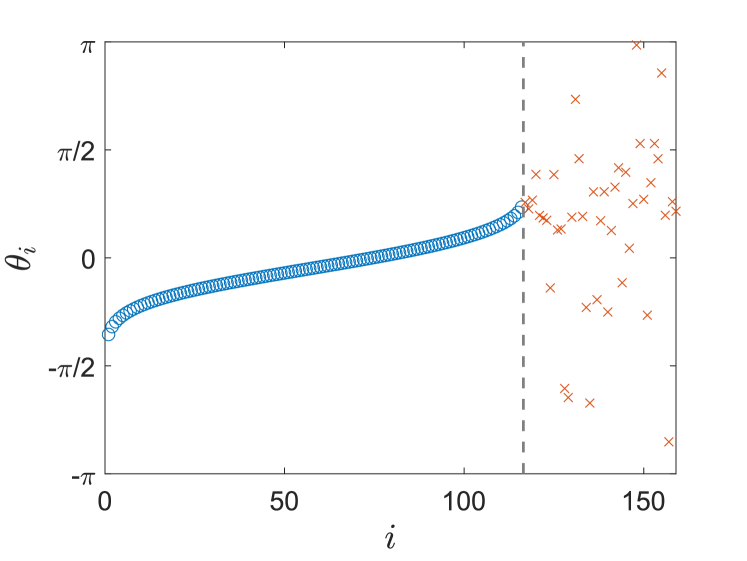
Figure 1a shows a snapshot of the phases for $N=160$. The phases are labelled according to their intrinsic frequencies such that the oscillator with the most negative native frequency is assigned the label $i=1$ and the one with the largest frequency the label $i=N$. One can see clearly the synchronised cluster with frequencies close to the mean frequency $\Omega$, and the non-entrained rogue oscillators with more extreme intrinsic frequencies. Note that due to the non-zero phase frustration $\lambda$ the synchronised cluster is not centred around the oscillators closest to the mean of their respective intrinsic frequencies as is the case for the standard Kuramoto model with $\lambda=0$. To determine the synchronised cluster and its complement, the non-entrained rogue oscillators, we define the effective frequency of each oscillator,

$$\hat{\omega}_{i}=\left\langle\dot{\theta}_{i}(t)\right\rangle_{t},$$

where the angular brackets denote a temporal average. Those oscillators with approximately the same effective frequencies $\hat{\omega}_{i}$ are considered to form the synchronised cluster $\mathcal{C}$ of size $N_{c}$, and the remaining oscillators are considered to be within the set of non-synchronised rogue oscillators $\mathcal{R}$ with size $N_{r}$. Figure 1b shows the effective frequencies.

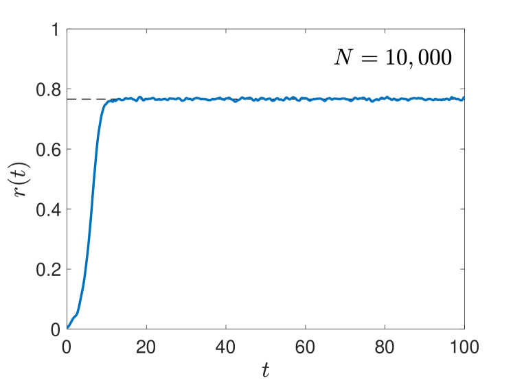
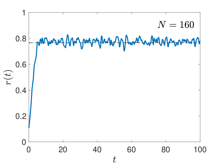
The effect of the non-collective behaviour of the rogue oscillators induces a seemingly stochastic behaviour of the order parameter $r$ shown in Figure 2. We show the temporal evolution of the order parameter from a random initial condition at $t=0$; after an initial transient the order parameter exhibits persistent fluctuations around a mean value with a constant variance of $4.16\times 10^{-4}$. The size of the fluctuations is $N$ dependent and we expect that for $N\to\infty$ the variance of the fluctuations approaches zero.

(a)

(b)

Figure 1: Snapshot of the phases $\theta_{i}$ (a) and effective frequencies $\hat{\omega}_{i}$ (b) for the Kuramoto-Sakaguchi model (1) with $N=160$ oscillators and phase frustration $\lambda=\frac{\pi}{4}$ at coupling strength $K=3$ with a Gaussian intrinsic frequency distribution with zero mean and unit variance. Circles (online blue) denote oscillators entrained in collective synchronised dynamics. Crosses (online red) denote the non-entrained rogue oscillators.

Figure 2: Time series of the order parameter $r(t)$ from a single simulation of the Kuramoto-Sakaguchi model (1) with $N=10,000$ and $N=160$ oscillators, starting from a random initial condition. The dashed horizontal line indicates the stationary value $r_{\infty}=0.766$ of the corresponding thermodynamic limit, estimated by solving the self-consistency relations (10)-(11). All parameters are the same as in Fig. 1.

To investigate the effect of finite system size, we simulate the system at increasing system size $N=\{40,80,160,320,640,1280,2560\}$ with other settings kept the same. Figure 3a shows the distribution of $r(t)$ for varying system size. As $N$ increases, the distribution of $r(t)$ becomes, as expected, narrower with decreasing variance and its mean value approaches a fixed value $\bar{r}_{\infty}=0.766$, as shown in Figures 3b-c. We find that $\bar{r}-r_{\infty}\sim N^{-0.859}$. The variance of $r(t)$ decreases towards 0 as $N$ increases with $\textrm{Var}[r]\sim N^{-0.976}$. The scaling of the variance suggests an underlying Central Limit Theorem which would imply a scaling of the variance with $1/N$.

(a)

(b)

(c)

Figure 3: (a): Empirical distribution of the order parameter $r(t)$ obtained from a single simulation of the Kuramoto-Sakaguchi model (1) at different system sizes $N$. (b): Mean value of $r(t)$ for different system sizes $N$. The dashed line indicates the value at the corresponding thermodynamic limit, $\bar{r}_{\infty}$. (c): Variance of $r(t)$ for different system sizes $N$. The red line represents the best-fit suggesting a scaling law of $N^{-0.976}$. All other parameters are the same as in Fig. 1.

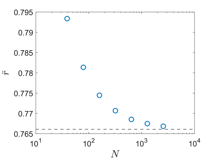
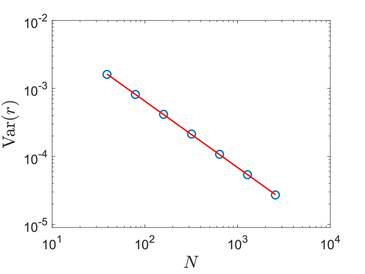
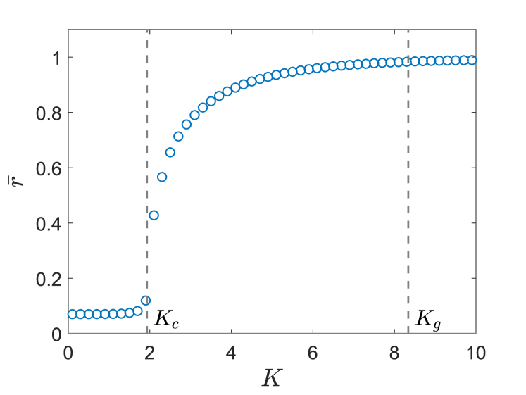
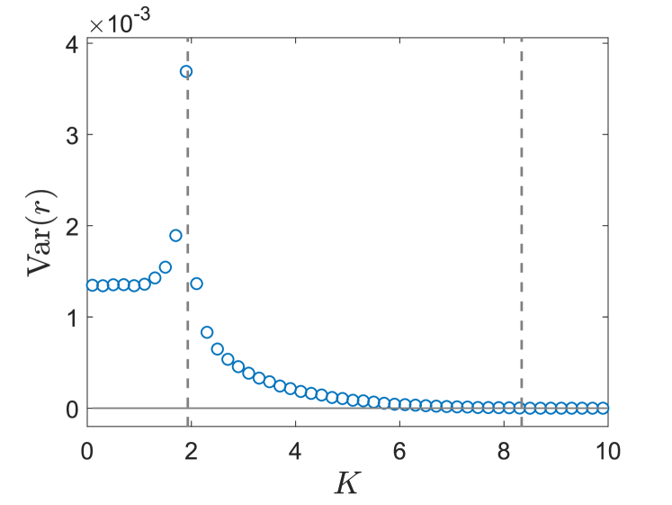
Figure 4 shows the well-known transition from incoherence to synchronisation for increasing coupling strength $K$ for a fixed number of oscillators $N=160$. Figure 4a shows the order parameter $\bar{r}$ with the well known second order phase transition for Gaussian intrinsic frequencies from incoherence with $\bar{r}\sim 1/\sqrt{N}$ to partial synchronisation at $K_{c}=1.93$, after which the synchronised cluster continues to grow in size until all oscillators become synchronised at $K_{g}=8.34$. Figure 4b shows the variance of the order parameter as a function of the coupling strength. The almost constant variance for small coupling strength around ${\rm{Var}}(r)=1.35\times 10^{-3}$ corresponds to the almost random distribution of the $N$ uncoupled oscillators. The variance exhibits a singularity at $K=K_{c}$ and approaches zero for $K\geq K_{g}$. The singular behaviour of the variance is a well-studied phenomenon and known under the name of anomalous enhancement of fluctuations [41, 42, 30, 43, 44, 31]. Figure 4c shows the cardinalities of the synchronised cluster $\mathcal{C}$ and the set of rogue oscillators $\mathcal{R}$, labelled $N_{c}$ and $N_{r}$, respectively, with $N_{c}+N_{r}=N$. For $K<K_{c}$ all oscillators are rogue whereas for $K>K_{g}$ all oscillators are synchronised. The synchronised cluster steadily grows for increasing $K_{c}<K<K_{g}$.

(a)

(b)

(c)

Figure 4: Transition from incoherence to synchronisation of the Kuramoto-Sakaguchi model (1) with increasing coupling strength $K$ with $N=160$ for a Gaussian intrinsic frequency distribution $g(\omega)$ with mean zero and variance $1$. (a): Order parameter $\bar{r}$. (b): Variance of the order parameter, quantifying the size of fluctuations. (c): Number of entrained oscillators $N_{c}$, which are part of the collective synchronised cluster (circles, online blue) and number of non-entrained rogue oscillators $N_{r}$ (crosses, online red). Shown are relative numbers. The vertical lines mark the onset of partial synchronisation at $K_{c}=1.93$ and the onset of global synchronisation at $K_{g}=8.34$.

III Stochastic model reduction

The numerical results presented in Section II.2 suggest that the non-entrained rogue oscillators exert a stochastic forcing on the synchronised cluster. To develop a stochastic approximation of the Kuramoto-Sakaguchi model we hence aim to establish a closed evolution equation for the phases of the synchronised oscillators in which the driving force exerted by the rogue oscillators is parametrised by a stochastic process. The challenge is how to describe this stochastic process. We begin by separating the coupling terms which only involve the synchronised oscillators and those which contain the rogue oscillators, and write the Kuramoto-Sakaguchi model (1) for $i\in\mathcal{C}$ as

$$\dot{\theta_{i}}=\omega_{i}-\Omega+\frac{K}{N}\left(\sum_{j\in\mathcal{C}}\sin(\theta_{j}-\theta_{i}-\lambda)+\sum_{j\in\mathcal{R}}\sin(\theta_{j}-\theta_{i}-\lambda)\right).$$

The sum over the rogue oscillators can be written as

$$\frac{1}{N}\sum_{j\in\mathcal{R}}\sin(\theta_{j}-\theta_{i}-\lambda)$$

$$\qquad=\frac{1}{N}\sum_{j\in\mathcal{R}}\sin(\theta_{j}-\psi_{c}+\lambda+\psi_{c}-\theta_{i}-2\lambda)$$

$$\qquad=\cos(\psi_{c}-\theta_{i}-2\lambda)\,S(t)+\sin(\psi_{c}-\theta_{i}-2\lambda)\,C(t),$$

where we introduced the mean phase of the synchronised cluster $\psi_{c}$ and where we define

$$S(t) =\frac{1}{N}\sum_{j\in\mathcal{R}}\sin(\theta_{j}-\psi_{c}+\lambda)=\frac{N_{r}}{N}r_{r}\sin(\psi_{r}-\psi_{c}+\lambda)$$ (12)

$$C(t) =\frac{1}{N}\sum_{j\in\mathcal{R}}\cos(\theta_{j}-\psi_{c}+\lambda)=\frac{N_{r}}{N}r_{r}\cos(\psi_{r}-\psi_{c}+\lambda),$$ (13)

where we defined the mean-field variables pertaining to the synchronized oscillators in $\mathcal{C}$

$$r_{c}e^{i\psi_{c}}=\frac{1}{N_{c}}\sum_{j\in\mathcal{C}}e^{i\theta_{j}}$$ (14)

and those pertaining to the rogue oscillators in $\mathcal{R}$

$$r_{r}e^{i\psi_{r}}=\frac{1}{N_{r}}\sum_{j\in\mathcal{R}}e^{i\theta_{j}}.$$ (15)

We remark that the particular choice of writing the trigonometric functions in (12)-(13) was motivated by the form of the invariant density of the rogue oscillators (8) and allows for a convenient averaging (cf. (17)-(19)). The overall influence of the rogue oscillators on each synchronised oscillator $\theta_{i}$ is now captured by $S(t)$ and $C(t)$, while the remaining terms are expressed entirely in terms of the synchronised oscillators, and we arrive at

$$\dot{\theta_{i}} =\omega_{i}-\Omega+\frac{K}{N}\sum_{j\in\mathcal{C}}\sin(\theta_{j}-\theta_{i}-\lambda)$$

$$+K\cos\tilde{\theta}_{i}\;S(t)+K\sin\tilde{\theta}_{i}\;C(t),$$ (16)

where we defined for compactness

$$\tilde{\theta}_{i}=\psi_{c}-\theta_{i}-2\lambda.$$

We first establish the average effect of the rogue oscillators and calculate the means $\langle S\rangle$ and $\langle C\rangle$ of the rogue oscillator drivers $S(t)$ and $C(t)$. We follow here the averaging procedure proposed in our previous work[36]. Envoking ergodicity of the process we can equate the temporal averages $\langle S\rangle$ and $\langle C\rangle$ by averages over the stationary density function of the rogue oscillators (8). Averaging equation (12) for $S(t)$ over the invariant densities of the rogue oscillators (8) becomes

$$\langle S\rangle_{t} \approx\frac{1}{N}\sum_{j\in\mathcal{R}}\,\int_{0}^{2\pi}\sin(\theta_{j}-\psi_{c}-\lambda)\rho(\theta_{j};\omega)d\theta_{j}$$

$$=\frac{1}{N}\cos(\psi-\psi_{c})\sum_{j\in\mathcal{R}}k_{j},$$ (17)

where

$$k_{j}=\frac{\omega_{j}-\Omega}{Kr}\left(1-\sqrt{1-\frac{K^{2}r^{2}}{(\omega_{j}-\Omega)^{2}}}\right),$$ (18)

and $\psi$ denotes the overall phase of all oscillators in the frame of reference rotating with the mean frequency $\Omega$. Similarly, averaging (13) yields

$$\langle C\rangle_{t}=-\frac{1}{N}\sin(\psi-\psi_{c})\sum_{j\in\mathcal{R}}k_{j}\approx 0,$$ (19)

since the overall phase $\psi$ and the phase of the synchronized cluster $\psi_{c}$ are close for sufficiently large coupling strength. In practice we estimate $\langle S\rangle_{t}$ and $\langle C\rangle_{t}$ from a long time trajectory. We confirmed that this is a good estimate for the thermodynamic limit.

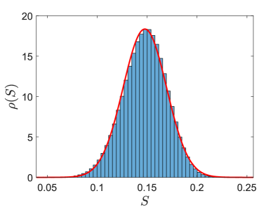
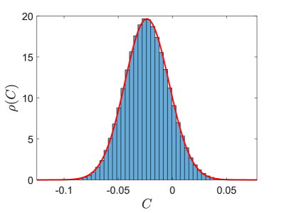
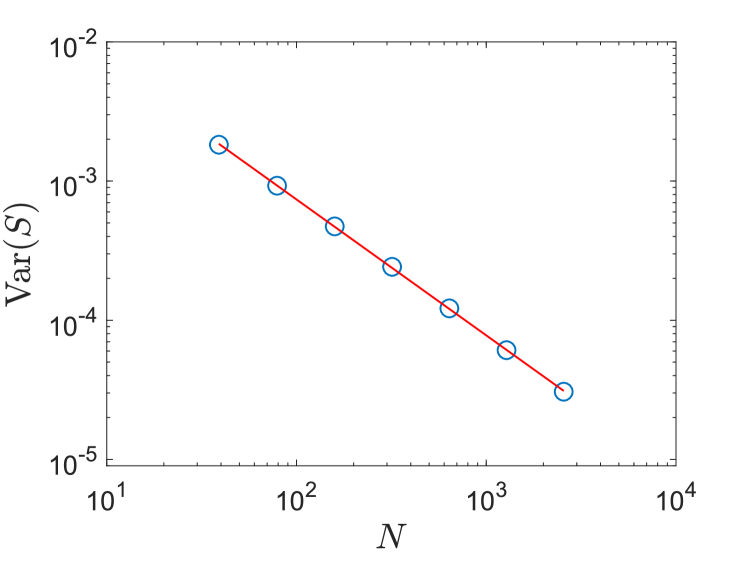
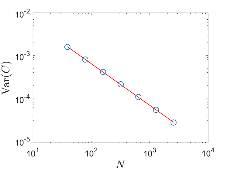
Figure 5 shows the empirical histogram of $S$ and $C$ for $N=160$ at $K=3$ obtained from a single long simulation of the Kuramoto-Sakaguchi model (1). The means are well approximated by the averaging procedure[36] described above (cf (17) and (19)). However, $S(t)$ and $C(t)$ experience significant fluctuations. It is clearly seen that the distribution of the fluctuations is Gaussian. In Figure 6 we show that the variance of $S$ and of $C$ scales approximately as $1/N$. This suggests that the scaled mean-subtracted variables

$$\xi_{t} =\sqrt{N}\left(S(t)-\langle S\rangle_{t}\right)+o(\frac{1}{\sqrt{N}})$$

$$\zeta_{t} =\sqrt{N}\left(C(t)-\langle C\rangle_{t}\right)+o(\frac{1}{\sqrt{N}})$$ (20)

are Gaussian processes that are defined entirely in terms of their mean and covariance functions

$$R_{ab}(\tau)={\rm{cov}}(a(t),b(t+\tau)),$$ (21)

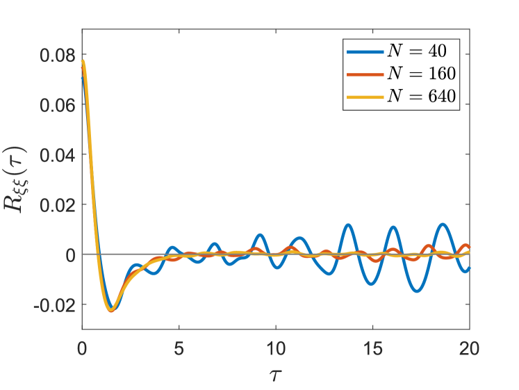
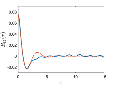
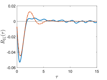
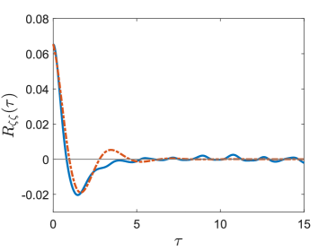
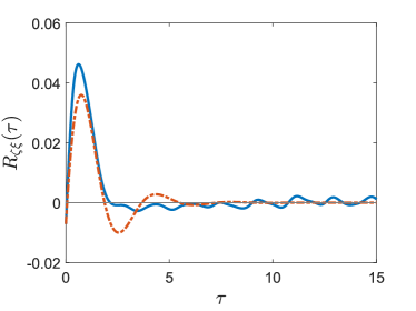
for $a$ and $b$ being either $\xi$ or $\zeta$. Indeed, Figure 7 shows that correlations decay in time with increasing system size $N$, and that the covariance functions of the scaled variables $\xi_{t}$ and $\zeta_{t}$ converge in the limit of $N\to\infty$. Note that the covariance functions of $\xi_{t}$ and $\zeta_{t}$ do not scale with $N$. This allows us to approximate $Z_{\rm{KS}}=(\xi_{t},\zeta_{t})^{T}$ as a two-dimensional Ornstein-Uhlenbeck process with

$$dZ=\left(-\Gamma Z+\Upsilon Z\right)dt+\Sigma\,dB_{t}$$ (22)

with two-dimensional Brownian motion $B_{t}=(W_{1},W_{2})$ and diagonal matrix $\Gamma=\gamma\,\mathrm{I}$ and skew-symmetric rotation matrix $\Upsilon$ with entries $\upsilon_{12}=-\upsilon_{21}=\upsilon$ and $\upsilon_{11}=\upsilon_{22}=0$ and a symmetric diffusion matrix $\Sigma$ with entries $\sigma_{ij}$ for $i,j=1,2$. The parameters of the Ornstein-Uhlenbeck process are determined such that its mean is zero and its covariance function

$$R^{(\rm{OU})}(\tau)=\langle e^{-(\Gamma-\Upsilon)\tau}Z_{0}Z_{0}^{T}\rangle_{\rm{OU}},$$ (23)

where the $Z_{0}$ are random variables drawn from the stationary density of the OU process and the angular brackets $\langle\cdot\rangle_{\rm{OU}}$ denote the average over that density, matches the observed covariance function (21) of $Z_{\rm{KS}}=(\xi_{t},\zeta_{t})$ associated with the full deterministic Kuramoto-Sakaguchi model. We perform a nonlinear least-square optimisation minimising the objective function

$$E(\gamma,\upsilon,\Sigma)=\sum_{a,b}\,\int_{t_{\rm{min}}}^{t_{\rm{max}}} ||R_{ab}(t)-{R_{ab}^{(\rm{OU})}}(t)||^{2}dt$$

$$+\beta\left(||R_{ab}(0)-{R_{ab}^{(\rm{OU})}}(0)||^{2}\right),$$

where the sum goes over all entries of the covariance matrix. We choose $\beta=1,000$ to enforce that the variances of $S$ and $C$ are reproduced. Figure 8 shows the four entries of the covariance matrix of $Z_{\rm{KS}}=(\xi_{t},\zeta_{t})$ together with the best fit of an OU process. The fit is significantly better for small times $\tau$. We remark that the Kuramoto-Sakaguchi model is deterministic and hence the derivatives of the covariance functions $R_{\xi\xi}(\tau)$ and $R_{\zeta\zeta}(\tau)$ are zero at $\tau=0$ [45]. This feature cannot be reproduced by the stochastic Ornstein-Uhlenbeck process which supports covariance functions that are non-differentiable at $\tau=0$; this suggest a lower integration bound $t_{\rm{min}}\neq 0$. We choose here $t_{\rm{min}}=0.5$ and $t_{\rm{max}}=2.5$.

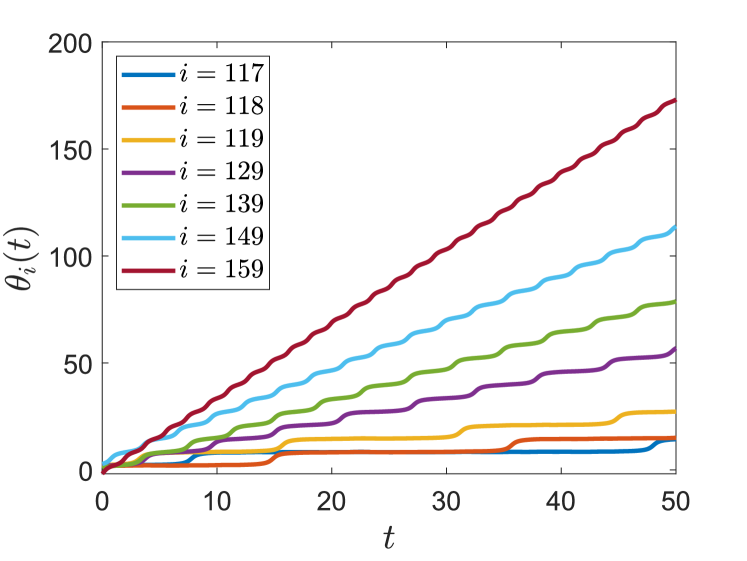
The effective stochastic dynamics of $S(t)$ and $C(t)$ are generated by the weak chaoticity of the non-entrained rogue oscillators [46, 47]. We show in Figure 9 typical trajectories of rogue oscillators. The dynamics of the weakly chaotic rogue oscillators is characterized by a nearly periodic motion (indeed under the assumption of constant mean-field variables $r$ and $\psi$ the dynamics of each rogue oscillator is approximately governed by the Adler equation (4)). Note that the rogue oscillators closest to the synchronized cluster evolve slowly, almost aligned with the synchronized cluster, for long periods interrupted by fast slips. The interaction terms (12) and (13) hence constitute sums of nearly periodic functions of time with random initial phases. It is well known that a sum of many trigonometric functions with uncorrelated random initial conditions approximates a Gaussian processes [48, 49, 50]. Hence the mechanism for the deterministic generation of diffusive behaviour is less a matter of the time-scale separation between faster chaotic rogue oscillators and slower synchronized oscillators (i.e. homogenization), but instead it is given by a weak coupling of the synchronized oscillators to many uncorrelated rogue oscillators.

Figure 5: Empirical histogram of $S(t)$ and $C(t)$ obtained from a single trajectory of the Kuramoto-Sakaguchi model (1) with $N=160$. The continuous curve (online red) shows the corresponding Gaussian best fit.

Figure 6: Scaling of the variance of $S$ and $C$ with varying system size $N$ as calculated from a single trajectory of the Kuramoto-Sakaguchi model (1). The continuous line is a linear best fit indicating a scaling with $N^{-0.977}$ and $N^{-0.975}$ for $S$ and $C$, respectively.

Figure 7: Entry $R_{\xi\xi}(\tau)$ of the covariance function of $Z_{\rm{KS}}=(\xi(t),\zeta(t))$ obtained from a single trajectory of the Kuramoto-Sakaguchi model (1) for different system sizes $N$.

Figure 8: Covariance functions of $\xi(t)$ and $\zeta(t)$ of the Kuramoto-Sakaguchi model (1) with $N=160$ (continuous lines, online blue), together with the covariance function of a fitted two-dimensional Ornstein-Uhlenbeck process (dashed lines, online red).

Figure 9: Top: Typical trajectories of rogue oscillators obtained from a single trajectory of the Kuramoto-Sakaguchi model (1) for $N=160$ including the rogue oscillators with the native frequency closest to that of an entrained oscillator with index $i=117$ and the rogue oscillator with the largest intrinsic frequency with index $i=159$. Bottom: Zoom into a shorter time window for the rogue oscillators which are closest to the synchronized cluster showing their weakly chaotic nature.

III.1 Numerical Verification of the Stochastic Reduced Model

We now show that the fluctuations of the order parameter as observed in Figure 2 can be captured by the closed stochastic evolution equation for the entrained oscillators $\theta_{i}$ with $i\in\mathcal{C}$, established in the previous Section which we summarize here as

$$d{\theta_{i}} =\big{[}\omega_{i}-\Omega+\frac{K}{N}\sum_{j\in\mathcal{C}}\sin(\theta_{j}-\theta_{i}-\lambda)\,$$

$$\qquad+K\cos\tilde{\theta}_{i}\;(\langle S\rangle_{t}+\frac{1}{\sqrt{N}}\xi_{t})$$

$$\qquad+K\sin\tilde{\theta}_{i}\;(\langle C\rangle_{t}+\frac{1}{\sqrt{N}}\zeta_{t})\;\big{]}dt,$$ (24)

where $\xi_{t}$ and $\zeta_{t}$ are the components of a $2$-dimensional OU process governed by

$$d\xi_{t} =-\gamma\xi_{t}\,dt+\upsilon\zeta_{t}\,dt+\sigma_{11}dW_{1}+\sigma_{12}dW_{2}$$

$$d\zeta_{t} =-\gamma\zeta_{t}\,dt-\upsilon\xi_{t}\,dt+\sigma_{21}dW_{1}+\sigma_{22}dW_{2}.$$ (25)

We remark that in the thermodynamic limit $N\to\infty$ we recover the deterministic evolution equation derived in [36]. We simulate this system using an Euler-Maruyama integrator with a time step of $dt=0.01$.

We can now establish expressions for the order parameters associated with the stochastic reduced system (24)-(25). The order parameter $r_{c}$ and the mean phase $\psi_{c}$ can be directly determined from simulations of (24)-(25). The full order parameter $r$ can be expressed as

$$re^{i\psi}=\frac{N_{c}}{N}r_{c}e^{i\psi_{c}}+\frac{N_{r}}{N}r_{r}e^{i\psi_{r}}.$$ (26)

Using the definitions for $S$ and $C$ (12)-(13) which imply

$$(C+iS)e^{-i\lambda}=\frac{N_{r}}{N}r_{r}\,e^{i(\psi_{r}-\psi_{c})},$$

we can express (26) in terms of the complex variable ${\mathcal{Z}}_{t}=C(t)+i\,S(t)$, where we treat ${\mathcal{Z}}_{t}$ now as a complex valued random variable, and obtain

$$r(t)=\left|\frac{N_{c}}{N}r_{c}(t)+{\mathcal{Z}}_{t}\,e^{-i\lambda}\right|.$$ (27)

We separate the mean part and the fluctuations of ${\mathcal{Z}}_{t}$ according to

$${\mathcal{Z}}_{t} =C(t)+i\,S(t)=\langle\mathcal{Z}\rangle+\frac{1}{\sqrt{N}}\mathcal{Z}^{\prime}_{t}$$

with $\langle\mathcal{Z}\rangle=\langle C\rangle+i\,\langle S\rangle$. The random variable ${\mathcal{Z}}^{\prime}_{t}$ is generated from the OU process (25) via the definition (20).

Note that this equation for $r$ is only an approximation as we require $r(t)\leq 1$ for all times $t$. The variance of the perturbing Ornstein-Uhlenbeck process ${\mathcal{Z}}^{\prime}_{t}/\sqrt{N}$ is much larger than that associated with the synchronised cluster, which we numerically verify as ${\rm{Var}}(r_{c})\approx 1.41\times 10^{-5}$ and ${\rm{Var}}(r_{r})\approx 6.5\times 10^{-3}$. This suggests that in the equation (27) for the order parameter $r(t)$ the stochasticity of $r_{c}$, as established above, can be neglected and we can approximate $r_{c}\approx\bar{r}_{c}={\rm{const}}$ and write

$$r(t)=\left|\bar{\rho}_{c}+\frac{1}{\sqrt{N}}{\mathcal{Z}}^{\prime}_{t}e^{-i\lambda}\right|,$$ (28)

with complex

$$\bar{\rho}_{c}=\frac{N_{c}}{N}\bar{r}_{c}+\langle\mathcal{Z}\rangle e^{-i\lambda}.$$ (29)

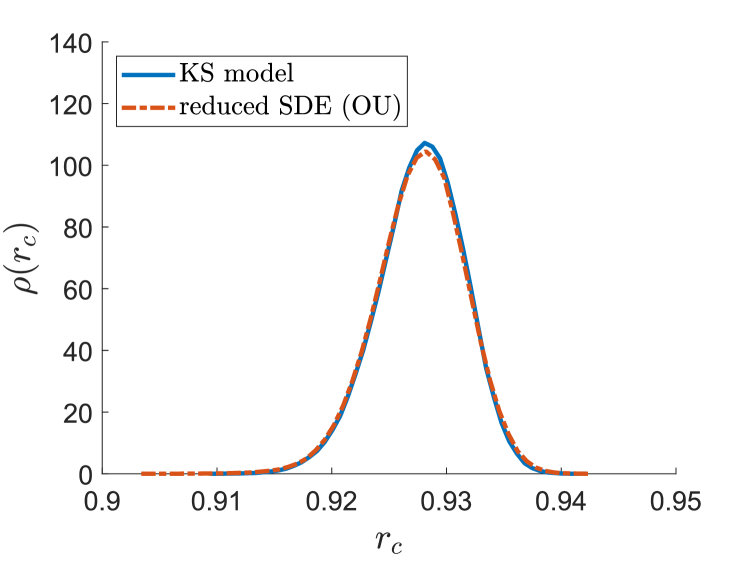
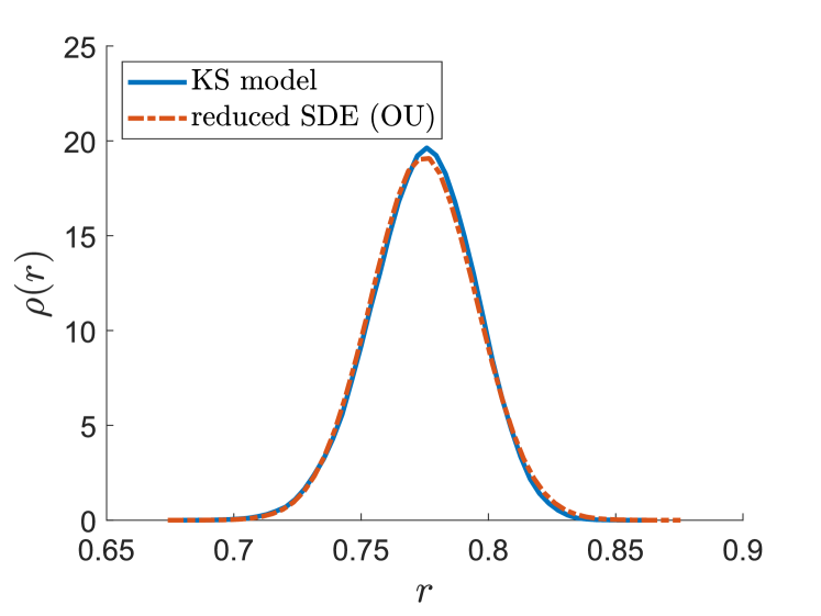
Figure 10 shows the empirical histograms of the order parameter $r_{c}$ pertaining to the synchronized oscillators as well as the total order parameter $r$ for all oscillators when simulated using the full Kuramoto-Sakaguchi model (1) with $N=160$ oscillators and when estimated by the reduced stochastic system (24)-(25) using (14) and (27) for the associated order parameters; we remark that results using the approximation (28) for the associated order parameter lead to results indistinguishable by eye. We further show the histogram of the order parameter $r_{c}$ which only takes into account the entrained synchronized oscillators. It is seen that our stochastic reduction captures the observed fluctuations for both $r_{c}(t)$ and $r(t)$ very well. We remark that the histograms are not distinguishable by eye if the order parameter is calculated by an actual time trajectory of $r_{c}(t)$ or by its constant mean $\bar{r}_{c}$ (cf. (27) and (28)).

Noting that the stochastic perturbations are small we can approximate further and write

$$r(t)=|\bar{\rho}_{c}|+\frac{1}{\sqrt{N}}{\rm{Real}}[\frac{\bar{\rho}_{c}}{|\bar{\rho}_{c}|}e^{-i\lambda}{\mathcal{Z}}_{t}^{\prime}],$$ (30)

which is equivalent to the following evolution equation for the order parameter

$$dr=\frac{1}{\sqrt{N}}{\rm{Real}}[\frac{\bar{\rho}_{c}}{|\bar{\rho}_{c}|}e^{-i\lambda}d{\mathcal{Z}}_{t}^{\prime}]$$ (31)

with

$$r(0)=|\bar{\rho}_{c}|,\;\;{\mathcal{Z}}^{\prime}(0)=0.$$ (32)

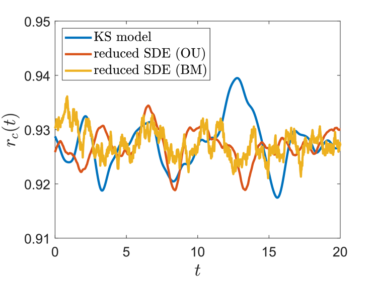
We remark that long-time solutions of (31) generate empirical histograms undistinguishable by eye from those presented in Figure 10. Note that the order parameter is driven by coloured noise in (31). This is in contrast to Snyder et al[37] who postulated Brownian motion as the driving noise. In Figure 11 we show the time evolution of the order parameter $r_{c}(t)$ computed from simulations of the full Kuramoto-Sakaguchi model (cf. Figure 2) and of our reduced stochastic system (24)-(25). It is seen that the qualitative smooth character of the fluctuations observed in the deterministic Kuramoto-Sakaguchi model (1) is reproduced by our stochastic system which is driven by coloured OU noise.

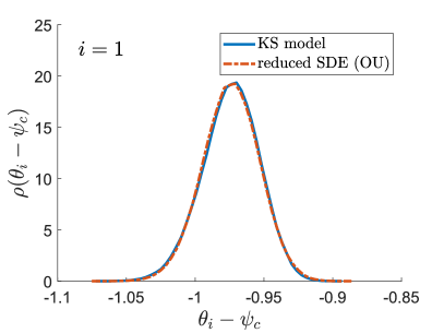
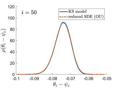
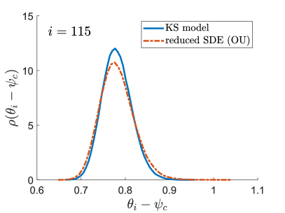
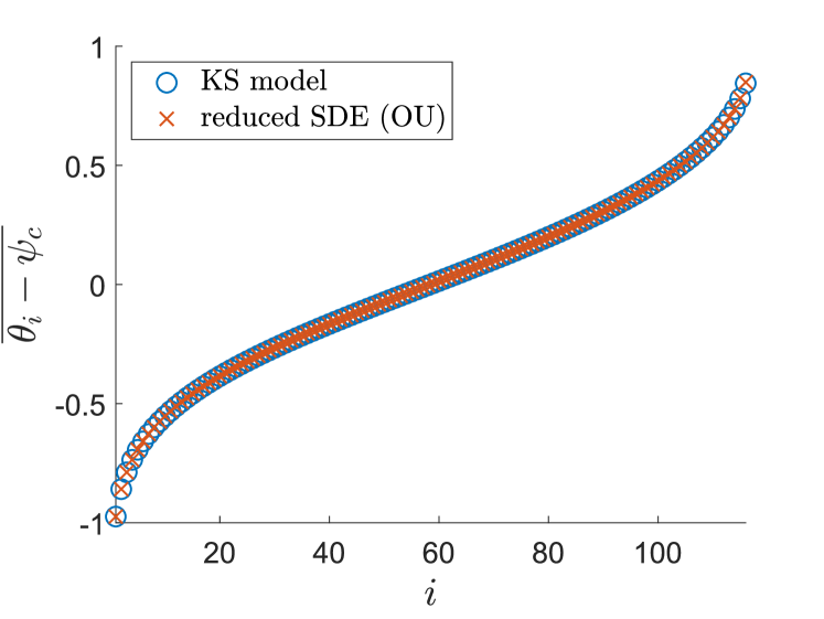
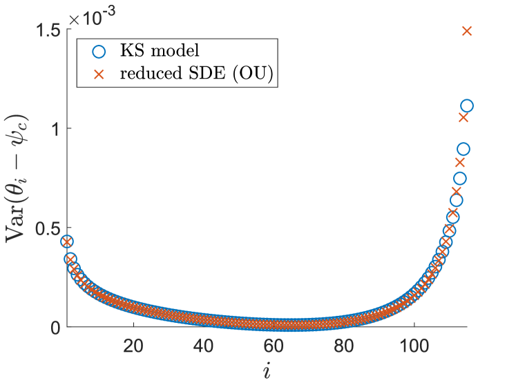
To further probe the ability of the reduced stochastic model (24)-(25) to capture the collective dynamics of the entrained synchronized oscillators we show results for the fluctuations of the entrained oscillators around the mean phase of the synchronized cluster, $\theta_{i}-\psi_{c}$ for $i\in\mathcal{C}$. These fluctuations are Gaussian for all entrained oscillators as shown in Figure 12. It is seen that our SDE very well describes entrained oscillators, such as those with indices $i=1$ and $i=50$, but the degree of approximation is less good for those entrained oscillators at the edge of the cluster with index $i=115$. In Figure 13 we show the mean and the variance of $\theta_{i}-\psi_{c}$ for all $i\in\mathcal{C}$ estimated from a long simulation of the full Kuramoto-Sakaguchi model (1) and of the reduced stochastic model (24)-(25). It is seen that the mean is very well recovered by the reduced stochastic model. The variance is very well captured for oscillators with an index $i$ that is sufficiently small to ensure that their intrinsic frequency is not too close to that of the closest rogue oscillator. For the simulations we show in Figure 13 the index of the first rogue oscillator is $i=117$ for the full Kuramoto-Sakaguchi model. The entrained oscillator with index $i=116$, i.e the oscillator on the edge of the synchronized cluster, is fully entrained in the Kuramoto-Sakaguchi model. However, for the approximate stochastic model (24)-(25) the oscillator with index $i=116$ experiences rare fast random slips between long periods of entrainment (of the order of $1,000$ time units on average). The rare and fast slips do not affect the mean which is still close to the mean corresponding to the Kuramoto-Sakaguchi model, but the variance is much higher with a value of $0.012$ (not shown in Figure 13 where we only show oscillators with index $i\leq 115$).

Figure 10: Comparison of the empirical histograms for $r_{c}$ (top) and $r$ (bottom) obtained from a single trajectory of the Kuramoto-Sakaguchi model (1) for $N=160$ and from the dynamics of the reduced stochastic model (24) driven by an OU process. All other parameters are the same as in Fig. 1.

Figure 11: Temporal evolution of the order parameter $r_{c}(t)$. Shown are results obtained from the full Kuramoto-Sakaguchi model (1) (online blue), the reduced stochastic model (24)-(25) driven by an OU process (online red) and from the Brownian motion approximation (39) (online orange). All other parameters are the same as in Fig. 1.

Figure 12: Empirical density of $\theta_{i}-\psi_{c}$ for the entrained oscillators with indices $i=1$, $i=50$ and $i=115$. Shown are results for the full Kuramoto-Sakaguchi model (1) for $N=160$ and for the reduced stochastic model (24)-(25). All other parameters are the same as in Fig. 1.

Figure 13: Mean (top) and variance (bottom) of the fluctuations of the entrained synchronized oscillators around their mean phase, $\theta_{i}-\psi_{c}$ for all $i\in\mathcal{C}$. Shown are results for the full Kuramoto-Sakaguchi model (1) for $N=160$ and for the reduced stochastic model (24)-(25). All other parameters are the same as in Fig. 1.

III.2 Approximation by Brownian motion: Homogenization results

A valid question is if one may model the effect of the rogue oscillators by Brownian motion instead of the more complex Ornstein-Uhlenbeck equation and describe the effective dynamics of the entrained synchronized oscillators by a single system of SDEs [37]?

In order to derive such a reduced SDE driven by Brownian motion we employ the method of homogenization. In particular, we treat the fluctuations, described by the Ornstein-Uhlenbeck process (25), as a fast process compared to the slow dynamics of the entrained synchronized oscillators, described by (24). Stochastic homogenization theory allows to derive an effective SDE for the slow variables (see, for example, [50, 51]).

We consider the fast-slow system

$$\dot{x} =a(x)+\epsilon^{-1}b(x)v(y)$$ (33)

$$dy =\epsilon^{-2}g(y)\,dt+\epsilon^{-1}dB,$$ (34)

where $x\in{\mathbb{R}}^{d}$ and $y\in{\mathbb{R}}^{q}$ and $B$ is $q$ dimensional Brownian motion. The functions

$$a:{\mathbb{R}}^{d}\to{\mathbb{R}}^{d},\quad b:{\mathbb{R}}^{d}\to{\mathbb{R}}^{d\times m},\quad v:{\mathbb{R}}^{q}\to{\mathbb{R}}^{m},\quad g:{\mathbb{R}}^{q}\to{\mathbb{R}}^{q},$$

and the drift and diffusion terms in the fast dynamics allow for a unique stationary density of the fast variables $\rho_{\infty}(y)$. We assume a centering condition $\int v(y)\,\rho_{\infty}(y)dy=0$. Note that our system (24)-(25) falls into this class of systems with $x$ denoting the synchronized oscillators with $d=N_{c}$ and $y$ denoting the two-dimensional OU process with $q=2$.

Homogenisation allows to find a limiting stochastic differential equation (SDE) for the slow variables in the limit $\epsilon\to 0$

$$dX=\tilde{a}(X)\,dt+b(X)\circ dW,$$ (35)

such that solutions $x$ of (33)-(34) converge weakly to $X$. Here, $W$ is $d$-dimensional Brownian motion, the stochastic integral $b(X)\circ dW$ has the Stratonovich interpretation, and $\tilde{a}$ is a modified drift term incorporating eventual corrections to the Stratonovich integral. Homogenization establishes that the Brownian motion $W$ has covariance matrix $\Sigma$ and the modified drift term is given by

$$\tilde{a}(X)=a(X)+\tfrac{1}{2}\sum_{\alpha,\beta,\gamma=1}^{d}E^{\gamma\beta}\partial_{\alpha}b^{\beta}(X)b^{\alpha\gamma}(X).$$ (36)

Here, $A^{ij}$ denotes the $(i,j)$’th entry of a matrix $A$ and $A^{\beta}$ denotes the $\beta$’th column of $A$. The symmetric and positive-definite covariance matrix $\Sigma$ is given by a Green-Kubo formula

$$\Sigma=\int_{0}^{\infty}\int\big{\{}v\otimes v_{t}+v_{t}\otimes v\big{\}}\,\rho_{\infty}(y)dy\,dt,$$ (37)

where $u\otimes v=uv^{T}\in{\mathbb{R}}^{d\times d}$ for $u,v\in{\mathbb{R}}^{d}$ and $v_{t}=v(y,t)=v(y(t);y(0)=y)$, and the so called Lévy area $E$ is given by the skew-symmetric matrix

$$E=\int_{0}^{\infty}\int\big{\{}v\otimes v_{t}-v_{t}\otimes v\big{\}}\,\rho_{\infty}(y)dy\,dt.$$ (38)

Identifying $b_{i}({\tilde{\theta}}_{i})=K\left(\cos(\tilde{\theta}_{i}),\,\sin(\tilde{\theta}_{i})\right)\in{\mathbb{R}}^{1\times 2}$ and $v=(S,\,C)^{T}\in{\mathbb{R}}^{2\times 1}$ we compute

$$\Sigma=2\int_{0}^{\infty}\begin{pmatrix}R^{(\rm{OU})}_{\xi\xi}(t)&0\\ 0&R^{(\rm{OU})}_{\zeta\zeta}(t)\end{pmatrix}dt,$$

where we used $R^{(\rm{OU})}_{\xi\zeta}(t)=-R^{(\rm{OU})}_{\zeta\xi}(t)$, and

$$E=2\int_{0}^{\infty}\begin{pmatrix}0&R^{(\rm{OU})}_{\xi\zeta}(t)\\ -R^{(\rm{OU})}_{\xi\zeta}(t)&0\end{pmatrix}dt.$$

It turns out that the Stratonovich correction

$$h_{i}=\frac{1}{4}\sum_{j=1}^{d}\sum_{k=1}^{2}\Sigma_{kk}\frac{\partial b_{ik}}{\partial\theta_{j}}({\tilde{\theta}}_{i})b_{jk}({\tilde{\theta}}_{j})=0$$

vanishes if we neglect derivatives of the mean phase $\psi_{c}$ with respect to $\theta_{i}$ and assume $\Sigma_{11}=\Sigma_{22}$ consistent with the numerical observations (cf. Figure 8). The drift correction associated with the Lévy area is calculated as $\delta\Omega:=KE^{12}/2=K\int_{0}^{\infty}R^{(\rm{OU})}_{\xi\zeta}(t)dt$. Note that this correction is a constant for all oscillators $i$, and hence only constitutes a correction to the global mean frequency $\Omega$. Summarizing, homogenization leads to the following SDE for the synchronized oscillators $i\in\mathcal{C}$ driven by Brownian motion

$$d{\theta_{i}} =\big{[}\omega_{i}-\tilde{\Omega}+\frac{K}{N}\sum_{j\in\mathcal{C}}\sin(\theta_{j}-\theta_{i}-\lambda)$$

$$+K\cos\tilde{\theta}_{i}\;\langle S\rangle_{t}+K\sin\tilde{\theta}_{i}\;\langle C\rangle_{t}\big{]}dt$$

$$+\frac{K}{\sqrt{N}}\Big{(}\cos\tilde{\theta}_{i},\;\,\sin\tilde{\theta}_{i}\Big{)}dW,$$ (39)

where $dW=(dW_{1}\;\;dW_{2})^{T}$ is two-dimensional Brownian motion with covariance matrix $\Sigma$ and $\tilde{\Omega}=\Omega-\delta\Omega$.

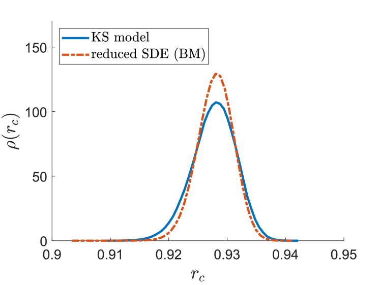
Figure 14 shows that the overall statistics of the order parameter $r_{c}$ is reasonably well described by the homogenized reduction (39), albeit to a lesser degree than with our stochastic reduced system (24)-(25). We remark that for the homogenized reduction (39) we are not able to define a meaningful expression for the overall order parameter $r$ as Brownian motion is a non-stationary process and the noise fluctuations $Z_{t}$ do not attain a constant variance (cf. (30)). Albeit the relatively good recovery of the statistical properties of the order parameter by the homogenized system, Figure 11 shows that its actual temporal evolution exhibits unrealistically non-smooth fluctuations (rather than by the smoother Ornstein-Uhlenbeck process).

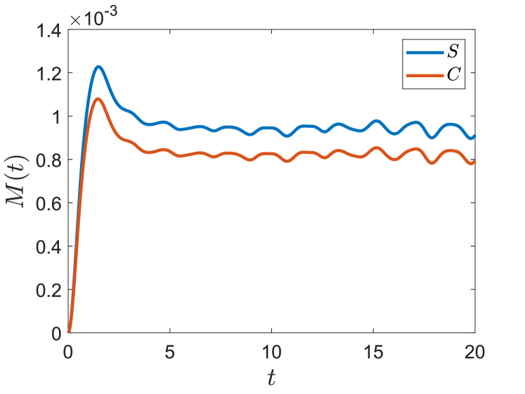
It is worthwhile to mention that the mean-square-displacement of $S(t)$ and $C(t)$, i.e.

$$M(t)=\lim_{T\to\infty}\frac{1}{T}\int_{0}^{T}(g(s+t)-g(s))^{2}ds,$$

for either $g(t)=S(t)$ or $g(t)=C(t)$, does not scale linearly with time $t$ as would be expected for Brownian motion, but instead saturates, in agreement with a stationary OU process, as shown in Figure 15.

These results agree with our earlier observation that the emerging stochastic behaviour of the dynamics of the entrained synchronized oscillators is not caused by a time-scale separation between slow synchronized cluster and the assumed fast rogue oscillators with larger intrinsic frequencies. We had already seen in Figure 9 that the dynamics of the rogue oscillators contains extended slow periods of near alignment with the synchronized cluster. Instead our work shows that the stochasticity emerges as a weak coupling effect of a large number of uncorrelated rogue oscillators.

Figure 14: Comparison of the empirical histograms for $r_{c}$ obtained from a single trajectory of the Kuramoto-Sakaguchi model (1) for $N=160$ and from the homogenized reduced stochastic model driven by Brownian motion (39). All other parameters are the same as in Fig. 1.

Figure 15: Mean-square-displacement $M(t)$ of $S(t)$ and $C(t)$. All parameters are the same as in Fig. 1.

IV Discussion

We provided a comprehensive treatment of the effect of non-entrained rogue oscillators on the collective behaviour of the entrained synchronized oscillators in the Kuramoto-Sakaguchi model. We established an average effect, in the spirit of a law of large numbers, and then determined the fluctuations around the mean effect akin to the central limit theorem. We presented results from numerical simulations that suggest that the fluctuations can be approximated by a Gaussian process with a stationary density and fluctuations which decay as $1/\sqrt{N}$. Hence for fluctuations to have a significant effect one needs the number of rogue oscillators to be sufficiently large to allow for a central limit theorem and sufficiently small to have a nonnegligible variance. Gaussian processes are determined entirely by their mean and their covariance function. This allowed us to replace the interaction term involving the rogue oscillators by an Ornstein Uhlenbeck process, and to formulate a closed equation for the entrained synchronized oscillators only, which are driven by this complex Ornstein-Uhlenbeck process. The reduced system of stochastic differential equations showed remarkable capability to reproduce the statistical behaviour of the entrained oscillators such as the probability density function of the order parameter. It is pertinent to mention that the order parameter is driven by coloured Ornstein-Uhlenbeck noise and not, as previously claimed on heuristic grounds, by Brownian motion. We showed that Brownian motion will lead to a far rougher time evolution of the order parameter than the actual Kuramoto-Sakaguchi equation. On a theoretical level, it would be interesting to see if one can employ homogenization theory for chaotic deterministic slow-fast systems [52, 53, 54, 55, 56] to derive limiting stochastic dynamics for the entrained oscillators directly from the deterministic Kuramoto-Sakaguchi model (1), assuming that rogue oscillators are fast. However, we caution that we showed here numerically that the fluctuations have an underlying stationary Gaussian distribution with a constant variance rather than a nonstationary Gaussian distribution with a linearly in time varying variance.

The stochastic reduced equation can now be further reduced, for example via the method of collective coordinates [33, 34, 47, 36, 35]. In particular, one can employ the methods developed for the reduction of a stochastic Kuramoto model [57] to the system derived here for the Kuramoto-Sakaguchi model. This has the potential to capture finite size effects which cannot be captured via standard mean-field theories.