Which Examples to Annotate for In-Context Learning? Towards Effective and Efficient Selection

Abstract

Large Language Models (LLMs) can adapt to new tasks via in-context learning (ICL). ICL is efficient as it does not require any parameter updates to the trained LLM, but only few annotated examples as input for the LLM. In this work, we investigate an active learning approach for ICL, where there is a limited budget for annotating examples. We propose a model-adaptive optimization-free algorithm, termed AdaIcl, which identifies examples that the model is uncertain about, and performs semantic diversity-based example selection. Diversity-based sampling improves overall effectiveness, while uncertainty sampling improves budget efficiency and helps the LLM learn new information. Moreover, AdaIcl poses its sampling strategy as a Maximum Coverage problem, that dynamically adapts based on the model’s feedback and can be approximately solved via greedy algorithms. Extensive experiments on nine datasets and seven LLMs show that AdaIcl improves performance by 4.4% accuracy points over SOTA (7.7% relative improvement), is up to $3\times$ more budget-efficient than performing annotations uniformly at random, while it outperforms SOTA with $2\times$ fewer ICL examples. Our code is available at https://github.com/amazon-science/adaptive-in-context-learning.

1 Introduction

Large Language Models (LLMs) have shown remarkable performance in various natural language tasks. One of the LLMs’ advantages is their ability to perform few-shot learning (Brown et al., 2020), where they can adapt to new tasks, e.g., topic classification or sentiment prediction, via in-context learning (ICL). ICL uses few-shot labeled examples $\{(x_{i},y_{i})\}_{i=1}^{k}$, e.g., $(x_{i},y_{i})=$ (Amazing movie!, positive), to construct a prompt $P$. Prompt $P$ is used as a new input to the LLM, e.g., “Amazing movie!: positive \n Awful acting: negative \n Terrible movie:”, before making predictions for the query $x_{\text{test}}$. The new input enables the LLM to infer the missing label $y_{\text{test}}$ by conditioning the generation on the few-shot examples. As semantically similar demonstrations to the test query improve ICL performance (Liu et al., 2021), it is common practice that a $k$-NN retriever is used to determine the $k$-nearest examples for each test query.

ICL is efficient as it does not require any parameter updates or fine-tuning, wherein users can leverage ICL to generate task-adaptive responses from black-box LLMs. However, ICL is sensitive to the input prompt (Lu et al., 2022) (the art of constructing successful prompts is referred to as prompt engineering), where acquiring ground-truth labeling of the input demonstrations is important for good ICL performance (Yoo et al., 2022). Ground-truth labeling requires expert annotators and can be costly, especially for tasks in which the annotators need to provide elaborate responses (Wei et al., 2022b). Apart from lowering the labeling cost, carefully reducing the number of the ICL examples can benefit inference costs and the LLM’s input context length requirements. Consequently, we study the following problem: Given a budget $B$, which examples do we select to annotate and include in the prompt of ICL?

Given an unlabeled set (pool) where we can draw ICL examples from, the above selection problem resembles a typical active learning setting Settles (2009); Zhang et al. (2022b). Active learning selects informative examples, e.g., via uncertainty sampling (Lewis & Gale, 1994), which are used to improve the model’s performance. Although traditional active learning involves model parameter updates, uncertainty sampling has been explored in an optimization-free manner for ICL with black-box LLMs (Diao et al., 2023; Pitis et al., 2023). Yet, recent studies show that uncertainty sampling yields inferior performance in comparison to other approaches (Margatina et al., 2023) and thus, current methods rely on semantic diversity to determine which examples are the most informative. For example, AutoCoT (Zhang et al., 2023b) performs clustering based on semantic similarity and selects the most representative examples of each cluster. In order to adapt the selection based on the LLM used, Vote$k$ (Su et al., 2022) selects diverse examples with respect to the LLM’s feedback, i.e., examples that the model is both uncertain and confident about. However, these approaches do not consider which examples help the LLM learn new information and may waste resources for annotating examples whose answers are already within the model’s knowledge.

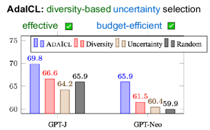
Figure 1: AdaIcl effectively combines diversity and uncertainty sampling, outperforming other strategies in the low-resource scenario, averaged over seven datasets. Here, the budget is 20 annotations for retrieval-based 5-shot ICL.

To overcome the aforementioned limitations of active learning for ICL, we pair uncertainty-based sampling with diversity-based sampling. To best combine the two sampling strategies, we propose a model-adaptive optimization-free method, termed AdaIcl, which is tailored to retrieval-based $k$-shot ICL. AdaIcl uses the LLM’s feedback (output probabilities) to identify the examples that the model is most uncertain about (hard examples). The algorithm then identifies different semantic regions of hard examples, with the goal to select the most representative examples within each region. Diversity-based sampling is posed as the well-studied Maximum Coverage problem (MaxCover), which can be approximately solved via greedy algorithms.

By selecting representative examples of diverse hard regions, AdaIcl aims for effectiveness, so that it helps the LLM learn information that it does not already know. Moreover, AdaIcl is efficient and results in budget savings by omitting the selection of examples that the model already knows how to tackle (easy examples). Finally, we show that AdaIcl’s uncertainty sampling improves the LLM’s calibration (Jiang et al., 2021; Zhao et al., 2021), i.e., how model’s confidence aligns with epistemic uncertainty, which measures how well the model understands the task.

We conduct experiments on nine datasets across five NLP tasks (topic classification, sentiment analysis, natural language inference, summarization, and math reasoning) with seven LLMs of varying sizes (1.3B to 65B parameters), including LLMs such as GPT-J (Wang & Komatsuzaki, 2021), Mosaic (MosaicML, 2023), Falcon (Penedo et al., 2023), and LLaMa (Touvron et al., 2023). Experimental results show that (i) AdaIcl is effective with an average performance improvement of 4.4% accuracy points over SOTA (Figure 1), (ii) AdaIcl is robust and achieves up to $3\times$ budget savings over random annotation, while it needs $2\times$ fewer ICL examples than SOTA (Section 6.2), and (iii) AdaIcl improves the calibration of the LLM’s predictions (Section 6.3).

2 Related Work

ICL Mechanism. In-context learning (ICL), also referred to as few-shot learning (Brown et al., 2020), has been shown to elicit reasoning capabilities of LLMs without any fine-tuning (Wei et al., 2022a; Bommasani et al., 2021; Dong et al., 2022). While ICL performance correlates to the pretraining data distribution (Xie et al., 2021; Hahn & Goyal, 2023; Shin et al., 2022; Razeghi et al., 2022; Chan et al., 2022) and improves with larger LMs (Bansal et al., 2023; Wei et al., 2023), recent works study how the transformer architecture (Vaswani et al., 2017) enables in-context learning (Akyürek et al., 2023; Olsson et al., 2022). Theoretical analyses and empirical studies show that ICL is a learning algorithm that acts as a linear regression (Akyürek et al., 2023; Garg et al., 2022; Von Oswald et al., 2023; Zhang et al., 2023a) and ridge (kernel) regression (Han et al., 2023; Bai et al., 2023) classifier. In this work, we leverage the recent connections of ICL with kernel regression to highlight the challenges of active learning for ICL.

Prompt Influence for ICL. Although ICL is widely used with LLMs, its success is not guaranteed as it is sensitive to the input prompts (Lu et al., 2022; Chen et al., 2022a). ICL tuning improves stability Min et al. (2022a); Chen et al. (2022b); Xu et al. (2023) but requires additional training data, while other works analyze how the prompt design and the semantics of the labels Min et al. (2022b); Yoo et al. (2022); Wang et al. (2022); Wei et al. (2023) affect ICL performance. More related to our setting, Liu et al. (2021),Rubin et al. (2022), Margatina et al. (2023), and Su et al. (2022) illustrate the importance of the $k$-NN retriever for ICL. Our work also highlights the importance of the $k$-NN retriever and provides new insights for improving ICL performance.

Active Learning for NLP. Active learning (Settles, 2009) for NLP has been well-studied (Zhang et al., 2022b) with applications to text classification (Schröder & Niekler, 2020), machine translation (Haffari et al., 2009), and name entity recognition Erdmann et al. (2019), among others. Ein-Dor et al. (2020) studied the application of traditional active learning techniques (Lewis & Gale, 1994; Sener & Savarese, 2018) for BERT pretrained models (Devlin et al., 2019), with many works following up (Margatina et al., 2021; Schröder et al., 2022). However, these approaches rely on LM fine-tuning, which can be more difficult to scale for larger models with tens of billions of parameters. Furthermore, most of the current approaches of active learning for ICL (Zhang et al., 2022a; Li & Qiu, 2023; Nguyen & Wong, 2023; Shum et al., 2023; Ma et al., 2023) assume a high-resource setting, where a large set of ICL examples is already annotated. This limits the applicability in practical low-resource scenarios (Perez et al., 2021), where annotations are costly to obtain.

3 Problem Statement & Motivation

Given an unlabeled set ${\mathcal{U}}=\{x_{i}\}_{i=1}^{N}$ and a fixed budget $B\in\mathbb{Z}^{+}$, the goal is to select a subset ${\mathcal{L}}\subset{\mathcal{U}}$, where ${\mathcal{L}}=\{(x_{i},y_{i})\}_{i=1}^{B}$ contains $B$ selected examples that are annotated. Due to token-length limits or inference cost considerations, we consider a $k$-shot ICL inference, where set ${\mathcal{L}}$ is used to draw $k$-shot ICL examples from ($k<B$). The $k$-shot examples are used to construct a new prompt $P$ as input to the LLM by

$$P=\pi(x_{1},y_{1})\oplus\pi(x_{2},y_{2})\oplus\cdots\oplus\pi(x_{k},y_{k})\oplus\pi(x_{\text{test}},*).$$ (1)

Template $\pi$ denotes a natural language verbalization for each demonstration $(x,y)$ and it also expresses how the labels $y$ map to the target tokens. The selected $B$ examples for set ${\mathcal{L}}$ should maximize the ICL model performance on the testing set.

To determine which ICL examples to use (and in which order), a $k$-NN retriever selects the top-$k$ examples from ${\mathcal{L}}$, e.g., $(x_{k},y_{k})$, for a test instance $x_{\text{test}}$ based on the similarity between $x_{i}\in{\mathcal{L}}$ and $x_{\text{test}}$ over a semantic space ${\mathcal{S}}$ (the order is determined by similarity scores). Employing a $k$-NN retriever for ICL example selection has demonstrated superior performance over random or fixed example selection  (Su et al., 2022; Margatina et al., 2023; Liu et al., 2021). We illustrate the overall problem setting in Figure 2.

To understand the impact of the ICL examples on model predictions, we express ICL inference as a non-parametric kernel regression, following the theoretical works from Han et al. (2023); Bai et al. (2023). The prediction for the test instance $x_{\text{test}}$ is related to

$$\tilde{y}_{\text{test}}=\frac{\sum_{i=1}^{k}y_{i}K_{\mathcal{D}}(x_{\text{test}},x_{i})}{\sum_{i=1}^{k}K_{\mathcal{D}}(x_{\text{test}},x_{i})},$$ (2)

where $K_{\mathcal{D}}(x_{\text{test}},x_{i})$ is a kernel that measures the similarity between $x_{\text{test}}$ with each of the $k$-shot retrieved instance $x_{i}$, which depends on the pretraining data distribution ${\mathcal{D}}$ for model $M$. The importance of the $k$-NN retriever in the lens of Equation 2 becomes clear: it fetches semantically similar examples to compute $\tilde{y}_{\text{test}}$ by regressing over their labels $y_{i}$. However, it does not account for which examples help the model learn the task to a larger extent, which depends on $K_{\mathcal{D}}$ and is infeasible to determine for pre-trained LLMs as there is usually no direct access to ${\mathcal{D}}$.

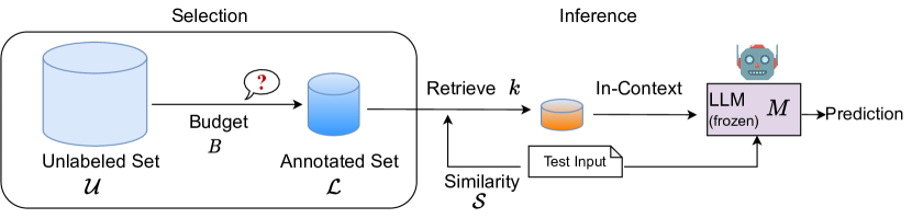
Figure 2: Our studied problem setting. Given an unlabeled set ${\mathcal{U}}$ and a fixed budget $B$, the goal is to select the $B$ most informative examples for annotation (set ${\mathcal{L}}$), which are used to maximize ICL performance with an LLM $M$. During ICL inference, a $k$-NN retriever based on a similarity space ${\mathcal{S}}$ determines the $k$-shot demonstrations for each test instance.

4 Adaptive Example Annotation for ICL

Can we improve example selection for ICL motivated by the aforementioned challenges? We answer affirmatively by putting forth a diversity-based uncertainty sampling strategy, termed AdaIcl, which adaptively identifies semantically different examples that help the model learn new information about the task.

The AdaIcl algorithm works as follows (see Figure 3 for an overview). First, it uses the LLM’s feedback to determine which examples the model is most uncertain about, which we refer to as hard examples. Then, it builds different regions of hard examples and the goal is to select the most representative example for each region. The regions are determined based on the semantic similarity space ${\mathcal{S}}$, apart from the LLM’s feedback, and denser regions are considered as more important.

By selecting representative examples of dense hard regions, we seek effectiveness by assuming that (i) these examples are informative for the hard examples that are close in the semantic space, and (ii) these examples will likely be retrieved during inference to improve predictions for similar hard examples (Equation 2). Moreover, by focusing on hard examples, we are interested in examples that the model is uncertain about in order to fill two needs. First, we seek budget-efficiency by avoiding annotating examples that the model already knows how to tackle, i.e., if $K_{\mathcal{D}}(x_{\text{test}},\cdot)$ is high. Second, we seek examples that the model is truly uncertain for and can help the model learn the task.

4.1 AdaIcl-base: A $k$means Approach

A straightforward solution is to perform $k$means clustering (MacQueen et al., 1967) over the identified hard examples for the model, where different clusters represent regions of hard examples.

To determine the set ${\mathcal{U}}_{h}$ of hard examples, we use the LLM’s feedback as follows. We assume we are given a small initially annotated pool ${\mathcal{L}}_{0}$ for $k$-shot ICL (if ${\mathcal{L}}_{0}=\emptyset$, we perform zero-shot ICL) and use the LLM $M$ to generate a prediction for each $x_{i}\in{\mathcal{U}}$. For classification problems, we compute the conditional probability of each class $y\in{\mathcal{Y}}$, and the label $\tilde{y}_{i}$ with the maximum conditional probability is returned as the prediction for $x_{i}$. Then, the probability score of the predicted label is regarded as the model’s confidence score $u_{i}$, where lower probability means that the model is less certain for its prediction $\tilde{y}_{i}$ (Min et al., 2022a). For generation problems, we average the log-probabilities of the generated tokens as the model’s confidence score $u_{i}$. We sort the examples $x_{i}\in{\mathcal{U}}$ based on their uncertainty scores $u_{i}$, and select the top-$N_{\theta}$ out of $N$ total examples, which are collected to ${\mathcal{U}}_{h}$. Here, $N_{\theta}=\lfloor\theta N\rfloor$ and $\theta\in[0,1]$ is a hyperparameter with default value $\theta=0.5$, which is the portion of the examples that we consider as hard ones.

Then, we can select representative examples for each region by sampling the example closest to each of the cluster centroids. Here, the number of clusters for $k$means is $B$, so we sample as many examples as the budget $B$ allows. We refer to that approach as AdaIcl-base and its algorithm is summarized in Appendix A.1. Yet, AdaIcl-base suffers from the known limitations of $k$means clustering. It is sensitive to outlier examples, which may be selected to be annotated, under the assumption that the $B$ regions formed by $k$means are equally important, and it does not account for the effect of overlapping clusters. We provide a failing case that the selected examples may not help the model understand the task in Appendix A.1.

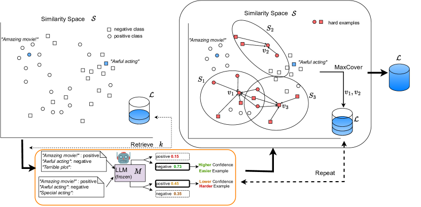
Figure 3: AdaIcl algorithm. AdaIcl uses $k$-shot ICL to determine which examples the model $M$ is uncertain for (hard examples). Then, it performs diversity-based uncertainty sampling over ${\mathcal{S}}$ by optimizing the MaxCover problem in Equation 3 via Algorithm 1 to identify the examples that help the model learn new information. The process is repeated until the budget $B$ is exhausted, and when done, it returns the annotated set ${\mathcal{L}}$.

4.2 AdaIcl: Selection by Maximum Coverage

AdaIcl overcomes the aforementioned limitations of AdaIcl-base by quantifying whether each each example can convey new information to the model. AdaIcl constructs semantic regions $S_{i}$ around every hard example $x_{i}$ and solves a Maximum Coverage (MaxCover) problem that accounts for information overlaps between different regions. MaxCover aims to select regions that cover the hardest examples, giving importance to denser regions and disregarding regions already covered (see Figure 3 for an overview).

Formally, MaxCover takes $m$ sets $\{S_{1},\dots,S_{m}\}$ (regions that contain semantically similar examples) and a number $B$ as input. Each set includes some examples, e.g., $S_{i}=\{x_{1},x_{2},\dots,x_{n}\}$ and different sets may have common examples, while the goal is to select the $B$ most representative sets that include (cover) as many examples as possible. We assume that if an example is marked as covered by another selected set, it conveys little new information to the model. In our setting, we are interested in hard examples, which we collect in the set ${\mathcal{U}}_{h}$ as previously explained. First, we discuss how we construct the regions and then we provide the MaxCover problem.

Set Construction. We represent the region $S_{i}$ around each example $x_{i}$ as its egonet. Initially, we build a global graph ${\mathcal{G}}_{m}$ as the $m$-nearest neighbors graph. The nearest neighbors are determined based on a semantic space ${\mathcal{S}}$ given by off-the-self encoders, such as SBERT (Reimers & Gurevych, 2019). We compute SBERT embeddings of each query $x_{i}$ and determine its neighbors based on cosine similarity of the embeddings. Graph ${\mathcal{G}}_{m}$ depends on the similarity space, while deriving sets $S_{i}$ from the global graph ${\mathcal{G}}_{m}$ depends on the LLM’s feedback as we are interested in hard examples $x_{i}\in{\mathcal{U}}_{h}$ for the model.

For every hard node $v\in{\mathcal{U}}_{h}$, we construct its 1-hop egonet. We consider edges that direct towards $v$ from other hard nodes $v^{\prime}\in{\mathcal{U}}_{h}$. This ensures that representative examples $x_{i}$, that are likely to be retrieved during ICL inference, have denser egonets. We experiment with both 1-hop and 2-hop set constructions. In the latter case, each node $v$ is represented by its egonet along with union of the egonets of its neighbors. One hyperparameter that controls the quality of the generated egonets is $m$, which is used during the construction of graph ${\mathcal{G}}_{m}$. In order to determine $m$, we employ a heuristic rule based on the desired maximum iterations $\hat{T}$ until the budget $B$ is exhausted, as well as the minimum number of hard examples $N_{\hat{\theta}}$ to be covered at each iteration. Due to space limitations, additional analysis of our approach are provided in Appendices A and D.

Greedy Optimization. The MaxCover problem is expressed as

maximize $$\sum_{x_{i}\in{\mathcal{U}}_{h}}c_{i},$$ (3)

where $$c_{j}\in\{0,1\},s_{i}\in\{0,1\},$$ (4)

subject to $$\;\sum s_{i}\leq B,\sum_{x_{j}\in S_{i}}s_{i}\geq c_{j}.$$ (5)

Equation 3 maximizes the coverage of the hard examples ${\mathcal{U}}_{h}$, indicator variable $c_{j}$ denotes if example $x_{j}$ is covered, and $s_{i}$ denotes if set $S_{i}$ is selected. The goal is to select the examples that convey new information to the model (measured by the indicator $c_{j}$). Equation 5 ensures that we select at most $B$ sets and covered examples belong to at least one selected set (the hard examples covered in more sets are selected before others). To adjust the problem in our scenario, selecting set $S_{i}$, i.e., MaxCover marks $s_{i}=1$, means that we select example $x_{i}$ for the annotated set ${\mathcal{L}}$.

The MaxCover problem is known to be NP-hard (Vazirani, 2001). A natural greedy solution for the MaxCover chooses sets according to one rule: at each stage, choose a set that contains the largest number of uncovered elements. This approximation algorithm is summarized below in Algorithm 1, and is well-known to approximately solve MaxCover and can be further improved due to its submodularity (Krause & Guestrin, 2005) .

Algorithm 1 Greedy approximation for MaxCover.

1:  Input: Examples ${\mathcal{U}}_{h}$, Sets $\{S_{1},\dots,S_{m}\}$, Budget $B$.

2:  while $B$ not exhausted do

3:     Pick the set that covers the most uncovered examples.

4:     Mark examples of the chosen set as covered.

5:  end while

Note that the greedy algorithm is terminated when every hard example is covered, regardless of whether the budget $B$ is exhausted. In this case, the selected examples are added to the annotation set ${\mathcal{L}}$, and the model’s feedback is re-evaluated to define the new hard set ${\mathcal{U}}^{\prime}_{h}$. The iterative process is terminated when the total budget $B$ is exhausted. The overall framework is summarized in Figure 3, and the algorithm is summarized in Appendix A.2.

4.3 AdaIcl+: Dynamically Re-Weighted MaxCover

The greedy Algorithm 1 for AdaIcl may cover all hard examples if the budget allows. However, this might include selecting sets that contain very few hard examples, e.g., outliers, or sets that belong to isolated sparse regions.

AdaIcl+ tackles this pitfall by a re-weighting schema for the MaxCover problem. Whenever a hard example is covered, instead of being marked as covered, AdaIcl+ reduces its weight. By having new weights, dense regions with hard examples are preferred over sparse regions if their total weight is greater. We provide such a case in Appendix A.2.

Unfortunately, dynamically updating the weights of each example does not satisfy the submodularity property of MaxCover, which is satisfied for fixed weights. Nevertheless, such that we can use the greedy algorithm to approximate the optimal solution, we propose a re-weighting trick by reusing ${\mathcal{U}}_{h}$ multiple times. Specifically, we copy the set ${\mathcal{U}}_{h}$ multiple times, i.e., to ${\mathcal{U}}^{0}_{h},{\mathcal{U}}^{1}_{h}$, etc., where different sets have different weights for their elements. If hard example $x_{i}$ is covered in ${\mathcal{U}}^{0}_{h}$, then we use its weights from the other sets. Formally, we optimize

$$\operatorname*{arg\,max}\sum_{t=0}^{\lfloor B/T\rfloor}\sum_{x^{t}_{i}\in U^{t}_{h}}w^{t}c^{t}_{i},$$ (6)

We set the weights $w^{t}$, so that $w^{t}\approx w^{t}+w^{t+1}+w^{t+2}+\cdots$, which can be achieved by exponentially reducing the weights. In our case, we set $w^{t}=10^{-t}$. In the beginning, every hard example of ${\mathcal{U}}^{0}_{h}$ has weight $w^{0}=1$ . If one example is covered in ${\mathcal{U}}^{0}_{h}$, i.e., $c^{0}_{i}=1$, then its new weight is obtained from ${\mathcal{U}}^{1}_{h}$, where $w^{1}=0.1$. We introduce a new hyperparameter $T$, which denotes the desired total number of iterations until we exhaust the budget. At each iteration, we can annotate $\lfloor B/T\rfloor$ new examples by solving Equation 6 and then, the model $M$ re-evaluates its predictions. AdaIcl+ algorithm is summarized in Appendix A.2.

5 Experimental Setting

With our experimental analysis, we address the following research questions (RQs):

• RQ1. How does AdaIcl compare with SOTA active learning strategies for ICL?

• RQ2. How efficient is AdaIcl regarding labeling and inference costs?

• RQ3. How robust is AdaIcl under different setups of the problem (Figure 2)?

• RQ4. Does AdaIcl help the LLM understand the task?

Datasets. We performed empirical evaluation with nine NLP datasets that cover well-studied tasks, such as topic classification (AGNews (Zhang et al., 2015), TREC (Hovy et al., 2001)), sentiment analysis (SST2 (Socher et al., 2013), Amazon (McAuley & Leskovec, 2013)), natural language inference (RTE (Bentivogli et al., 2009), MRPC (Dolan et al., 2004), MNLI (Williams et al., 2018)), text summarization (XSUM (Narayan et al., )) and math reasoning (GSM8K (Cobbe et al., 2021)). We provide examples of these datasets and additional details in Appendix B.

Baselines. We use the following approaches as baselines for comparison: (i) Random performs random example selection for annotation. (ii) Pseudo-labeling uses the LLM to generate pseudo-labels for the unlabeled instances as additional annotated data. (iii) Fast-vote$k$ (Su et al., 2022) is a diversity-based sampling strategy that selects representative examples in the similarity space. (iv) Vote$k$ (Su et al., 2022) additionally accounts for the model’s feedback. It sorts the examples based on the model’s confidence scores and stratifies them into $B$ equally-sized buckets. It selects the top-scoring fast-vote$k$ example from each bucket. (v) Hardest resembles the uncertainty sampling strategy of active learning. The examples that the model is the most uncertain for are selected. Additionally, we include (vi) AdaIcl-base method (Section 4.1) as further ablations.

(a) Topic Classif. (AGNews, TREC)

(b) Sentim. Analysis (SST2, Amazon)

(c) Nat. Lang. Inf. (RTE, MRPC, MNLI)

	Falcon-40B	LLaMa-65B
	Summarization (RougeL)
Zero-shot	$18.50_{\pm 0.61}$	$15.26_{\pm 0.69}$
Vote$k$	$20.83_{\pm 0.05}$	$23.38_{\pm 0.84}$
AdaIcl	$21.42_{\pm 0.68}$	$24.67_{\pm 0.45}$
	Math Reasoning (Accuracy)
Zero-shot	$36.58_{\pm 3.14}$	$32.54_{\pm 1.86}$
Vote$k$	$37.23_{\pm 1.75}$	$45.04_{\pm 1.47}$
AdaIcl	$39.58_{\pm 3.01}$	$49.08_{\pm 2.89}$

(d) Generation Tasks (XSUM, GSM8K)

Figure 4: Performance comparison across different tasks with GPT-J (6B) and GPT-Neo (1.3B). “Best Base.” denotes the best baseline for the task. AdaIcl performs the best, while for the classification tasks AdaIcl-base is the second-best (full results in Appendix C.1).

Design Space. As summarized in Figure 2, the design space includes the unlabeled set ${\mathcal{U}}$, the number of ICL examples $k$, the similarity space ${\mathcal{S}}$, the budget $B$, and the LLM $M$. We experiment with seven LLMs of varying sizes (1.3B to 65B parameters), including GPT, Mosaic, Falcon, and LLaMa model families, all of which are open-source and allow the reproducibility of our research. Unless otherwise stated, we set $k=5$, $B=20$ and we obtain embeddings in the similarity space via SBERT (Reimers & Gurevych, 2019). We experiment with inductive settings, where test instances come from an unseen set ${\mathcal{U}}_{\text{test}}$, but also for transductive settings, where test instances come from ${\mathcal{U}}$.

AdaIcl. For the default problem setup, we construct 2-hop sets with $m=5$ for AdaIcl, and 1-hop sets with $m=15$ for AdaIcl+ via Equation 7. The default number of iterations $T$ for AdaIcl+ is $T=2$, while in the additive budget scenario we have $T=1$. As the threshold hyper-parameter $\theta$, we have $\theta=0.5$, i.e., 50% of the examples are considered as hard. Hyper-parameter sensitivity studies that show AdaIcl’s robustness are presented in Appendix D.

6 Results & Analysis

6.1 RQ1: AdaIcl is Effective

Figures 4(a), 4(b), and  4(c) show performance results for classification tasks with two different models GPT-J (6B) and GPT-Neo (1.3B). AdaIcl is the method that achieves the best performance, with an improvement of up to 7.5% accuracy points over random selection. The overall improvement over the best baseline is 1.9% points for GPT-J and 3.2% for GPT-Neo, which shows that AdaIcl is important for smaller sized LMs. The second best performing method for topic classification and sentiment analysis is AdaIcl-base, which shows the importance of diversity-based uncertainty sampling for ICL. Figure 4(d) provides results for generation tasks. On the challenging reasoning tasks, AdaIcl outperforms Vote$k$ and zero-shot ICL by 4.04% and 16.54% in accuracy, respectively.

Figure 5: Multi-step results with GPT-Neo. Sweet point: the point at which we exceed the best performance achieved by random selection.

6.2 RQ2 & RQ3: AdaIcl is Efficient and Robust

Budget-Efficiency. We experiment with a scenario similar to mini-batch active learning, where the budget increases in different steps and the retriever uses as many ICL annotated examples as the context-length limit allows. Figure 5 shows results when incrementing the budget with 10 more annotations (for 4 steps). AdaIcl performs the best in all cases, where the average accuracy improvement over the best baseline is 7.09% for topic classification, 3.08% for sentiment analysis, and 2.36% for natural language inference. Figure 5 also shows that for topic classification and sentiment analysis AdaIcl exceeds the best performance achieved by random annotation with $3\times$ less budget.

Table 1: Impact of the number of ICL examples.

	GPT-J (6B)		Mosaic (7B)
	AGNews	SST2	AGNews	SST2
Vote$k$ 5-shot	$53.61_{\pm 7.72}$	$72.89_{\pm 11.67}$	$71.04_{\pm 8.12}$	$80.98_{\pm 5.26}$
Vote$k$ 10-shot	$58.32_{\pm 2.74}$	$80.08_{\pm 7.43}$	$76.09_{\pm 3.37}$	$90.23_{\pm 0.31}$
AdaIcl 5-shot	$67.44_{\pm 4.57}$	$83.98_{\pm 1.10}$	$77.20_{\pm 3.42}$	$89.58_{\pm 1.75}$

• $B=5$ and $B=10$ for 5-shot and 10-shot ICL, respectively.

Impact of ICL examples. Table 1 investigates AdaIcl’s efficiency with respect to the number of ICL examples used during inference (and annotated). As shown, AdaIcl outperforms vote$k$ although it uses and annotates $2\times$ fewer ICL examples. This indicates that AdaIcl identifies examples that help the LLM learn the task, while it can reduce the inference costs due to shorter input prompts. We provide a visualization of AdaIcl’s process in Appendix E.

Retriever Effect. Table 2 shows results when we use different off-the-shelf encoders for the similarity space ${\mathcal{S}}$, such as BERT (Devlin et al., 2019) and RoBERTa (Liu et al., 2019). As discussed in Section 3, it is difficult to approximate the true similarity between examples based on the pretraining distribution ${\mathcal{D}}$, and thus different encoders lead to different results. For example, SBERT achieves a maximum average performance of 55.33% and 77.73% for TREC and Amazon, respectively, while BERT achieves 44.06% and 85.80%. Despite the encoder choice, AdaIcl performs overall the best as its diversity-based uncertainty sampling mitigates this effect.

Figure 6: Average results over AGNews, TREC, SST2, and Amazon datasets for four LLMs with similar size.

LLM Effect. Figure 6 shows results when using different LLMs of similar sizes (6-7B parameters). The best performance is achieved for the Mosaic and GPT-J models. LLaMa does not display effective ICL capabilities and Falcon does not substantially improve with more annotated examples. For Mosaic and GPT-J models, AdaIcl outperforms Vote$k$ by 4.09% accuracy points, while the average accuracy improvement over random annotation for different budgets is 5.45% points.

Table 2: Performance comparison across different retrieval and semantic similarity configurations.

Retriever, ${\mathcal{S}}\xrightarrow{}$	SBERT-all-mpnet-base-v2			RoBERTa-nli-large-mean-tokens			BERT-nli-large-cls-pool			Avg.
	TREC	SST2	Amazon	TREC	SST2	Amazon	TREC	SST2	Amazon
Pseudo-labeling	$48.56_{\pm 6.33}$	$69.13_{\pm 3.87}$	$70.96_{\pm 3.35}$	$33.98_{\pm 3.68}$	$74.08_{\pm 4.40}$	$81.11_{\pm 4.14}$	$41.27_{\pm 4.24}$	$77.47_{\pm 1.60}$	$81.63_{\pm 2.49}$	$64.24$
Random	$54.68_{\pm 1.68}$	$68.48_{\pm 1.87}$	$73.95_{\pm 2.03}$	$37.23_{\pm 2.30}$	$74.21_{\pm 3.50}$	$84.46_{\pm 3.21}$	$34.75_{\pm 2.41}$	$72.65_{\pm 5.82}$	$80.20_{\pm 3.34}$	$64.51$
Vote$k$	$54.81_{\pm 0.49}$	$73.69_{\pm 9.05}$	$75.13_{\pm 0.98}$	$37.77_{\pm 4.65}$	$76.16_{\pm 2.23}$	$84.11_{\pm 1.28}$	$42.43_{\pm 3.34}$	$80.85_{\pm 2.09}$	$83.59_{\pm 1.77}$	$67.61$
AdaIcl-base	$48.24_{\pm 0.98}$	$77.86_{\pm 1.02}$	$75.77_{\pm 3.63}$	$38.12_{\pm 5.74}$	$78.12_{\pm 5.30}$	$\underline{85.93}_{\pm 2.30}$	$38.15_{\pm 3.10}$	$78.64_{\pm 2.78}$	$\underline{85.80}_{\pm 1.75}$	$67.40$
AdaIcl	$\underline{55.33}_{\pm 2.57}$	$\underline{79.68}_{\pm 2.47}$	$\underline{77.73}_{\pm 2.23}$	$\underline{39.06}_{\pm 3.37}$	$\underline{81.11}_{\pm 1.50}$	$85.15_{\pm 0.55}$	$\underline{44.06}_{\pm 2.49}$	$\underline{80.85}_{\pm 2.83}$	$84.65_{\pm 3.52}$	69.74

6.3 RQ3: AdaIcl improves Calibration

One motivation behind uncertainty sampling is that it helps the LLM understand the task. Our hypothesis is that selecting examples that the LLM is over-confident for, i.e., easy examples, might not convey new information for the LLM to truly understand the task. We test our hypothesis by introducing a new variant of our method, termed AdaIcl-easy, which constructs regions of hard examples around easy examples for MaxCover. To compare AdaIcl-easy with our original AdaIcl-hard, we compute the expected calibration error (ECE) (Guo et al., 2017) which quantifies the discrepancy between a model’s predicted probabilities (how well it believes it understands the task) and observed outcomes (how well it actually solves the task). In addition, we visualize the discrepancy across probability bins by reliability plots, where any deviation from the straight diagonal indicates miscalibration and misunderstanding of the task.

As shown in Figure 7, “phase changes” in ECE could be observed for AdaIcl-hard at different iterations and thus, improved calibration. We conjecture that the over-confident examples selected using AdaIcl-easy lead to the bias towards making over-confident ICL predictions that are not always true. This is verified by the reliability plots for two snapshots: at iteration=7 for AGNews and at iteration=2 for SST2, where AdaIcl-hard reduces the ECE from 0.20-0.30 to approximately 0.1. AdaIcl-easy tends to make over-confident predictions (heavily skewed towards the right of the x-axis and large deviation from the diagonal), whereas AdaIcl-hard produces more calibrated predictions, with more uniform probability distributions. We provide additional calibration analysis in Appendix C.4.

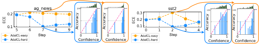
Figure 7: Expected calibration errors (ECE – the lower the better) and reliability plots for AdaIcl when selecting easy (AdaIcl-easy) and selecting hard (AdaIcl-hard) examples.

7 Conclusions

In this work, we investigated budgeted example selection for annotation for ICL, a previously under-explored area. Seeking for an effective and efficient selection, we introduce AdaIcl, a diversity-based uncertainty selection strategy. Diversity-based sampling improves effectiveness, while uncertainty sampling improves budget efficiency and helps the LLM learn new information about the task. Extensive experiments in low-resource settings show that AdaIcl outperforms other approaches in five NLP tasks using seven different LLMs. Moreover, AdaIcl can result into considerable budget savings, while it also needs fewer ICL examples during inference to achieve a given level of performance, reducing inference costs. Finally, our calibration analysis showed that AdaIcl selects examples that lead to well-calibrated predictions.

8 Reproducibility Statement

The code of our AdaIcl algorithm is at https://github.com/amazon-science/adaptive-in-context-learning. AdaIcl’s algorithmic steps are extensively summarized in Appendix A. For the datasets used, a complete description of the data processing steps is given in Appendices B.1 and B.2. Details of the experimental configurations are given in Appendix B.3.

Appendix

Appendix A AdaIcl Details

A.1 AdaIcl-base

Algorithm 2 presents the overall AdaIcl-base algorithm. First, AdaIcl-base uses the LLM’s feedback to identify hard examples for the model based on their uncertainty scores. Then, it performs $k$means clustering where different clusters represent regions of hard examples and selects representative examples for each region by sampling the example closest to each of the cluster centroids. Here, the number of clusters for $k$means is $B$, so that we sample as many examples as the budget $B$ allows.

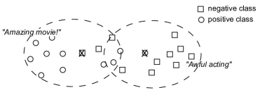
Figure 8: Failing case for $k$means clustering.

AdaIcl-base suffers from the known limitations of $k$means clustering. It is sensitive to outlier examples, which may be selected to be annotated, assumes that the $B$ formed regions are equally important, and does not account for the effect of overlapping clusters. We provide such a failing case in Figure 8. Here, the annotated examples (with $B=2$) do not effectively represent the semantic space and may not help the model understand the task.

Algorithm 2 AdaIcl-base Algorithm.

1:  Input: Model $M$, Unlabeled Set ${\mathcal{U}}$, Budget $B$, Similarity Space ${\mathcal{S}}$ for $k$-NN Retriever.

2:  Optional: Initial set ${\mathcal{L}}_{0}$, else ${\mathcal{L}}_{0}=\emptyset$.

3:  Hyperparameters: threshold $\theta$.

4:  Output: Annotated Set ${\mathcal{L}}$.

5:  for  $x_{i}\in{\mathcal{U}}$ do

6:     Retrieve (at most) $k$ examples from ${\mathcal{L}}$ based on similarity ${\mathcal{S}}$.

7:     Use model $M$ to obtain an uncertainty score $u_{i}$ for $x_{i}$ with $k$-shot ICL.

8:  end for

9:  Determine hard set ${\mathcal{U}}_{h}$ given scores $\{u_{i}\}$ and threshold $\theta$.

10:  Perform $k$means clustering of ${\mathcal{U}}_{h}$ into $B$ clusters with centroids $\{\mu_{j}\}_{j=1}^{B}$.

11:  for  $j=1,\dots,B$ do

12:     $x^{\ast}_{i}=\operatorname*{arg\,min}_{x_{i}\in{\mathcal{U}}_{h}}||\mu_{j}-x_{i}||$.

13:     Add the selected $x^{\ast}_{i}$ to ${\mathcal{L}}={\mathcal{L}}\cup\{x^{\ast}_{i}\}$ and remove it from ${\mathcal{U}}_{h}={\mathcal{U}}_{h}\setminus\{x^{\ast}_{i}\}$.

14:  end for

A.2 AdaIcl Algorithms

Algorithm 3 summarizes the overall AdaIcl algorithm, and Algorithm 4 summarizes the overall AdaIcl+ algorithm. Their key differences are the following. First, AdaIcl solves a MaxCover problem (Line 14), while AdaIcl solves a weighted MaxCover problem (Line 14). Second, AdaIcl+ performs a predefined number of iterations $T$ (Line 7), sampling a fixed number of examples $B_{cur}=\frac{B}{T}$ (Line 14) per iteration. AdaIcl is repeated until termination (Line 7), where the number of selected examples per iteration is determined by the MaxCover (Line 14) solution.

Algorithm 3 AdaIcl Algorithm.

1:  Input: Model $M$, Unlabeled Set ${\mathcal{U}}$, Budget $B$, Similarity Space ${\mathcal{S}}$ for $k$-NN Retriever.

2:  Optional: Initial set ${\mathcal{L}}_{0}$, else ${\mathcal{L}}_{0}=\emptyset$.

3:  Hyperparameters: threshold $\theta$, number of neighbors $m$.

4:  Output: Annotated Set ${\mathcal{L}}$.

5:  $B_{cur}=0,{\mathcal{L}}={\mathcal{L}}_{0}$.

6:  Create global graph ${\mathcal{G}}_{m}$.

7:  while $B_{cur}<B$ do

8:     for  $x_{i}\in{\mathcal{U}}$ do

9:        Retrieve (at most) $k$ examples from ${\mathcal{L}}$ based on similarity ${\mathcal{S}}$.

10:        Use model $M$ to obtain an uncertainty score $u_{i}$ for $x_{i}$ with $k$-shot ICL.

11:     end for

12:     Determine hard set ${\mathcal{U}}_{h}$ given scores $\{u_{i}\}_{i=1}^{N}$ and threshold $\theta$.

13:     Create sets $S_{i}$ given ${\mathcal{U}}_{h}$ and ${\mathcal{G}}_{m}$.

14:     $\{x^{\ast}_{i}\}_{i=1}^{B^{\ast}}$ = Greedy-MaxCover (${\mathcal{U}}_{h},\{S_{i}\},B-B_{cur}$).

15:     Add the selected $\{x^{\ast}_{i}\}_{i=1}^{B^{\ast}}$ to ${\mathcal{L}}={\mathcal{L}}\cup\{x^{\ast}_{i}\}_{i=1}^{B^{\ast}}$ and remove them from ${\mathcal{U}}={\mathcal{U}}\setminus\{x^{\ast}_{i}\}_{i=1}^{B^{\ast}}$.

16:     $B_{cur}=B_{cur}+B^{\ast}$.

17:  end while

Algorithm 4 AdaIcl+ Algorithm.

1:  Input: Model $M$, Unlabeled Set ${\mathcal{U}}$, Budget $B$, Similarity Space ${\mathcal{S}}$ for $k$-NN Retriever.

2:  Optional: Initial set ${\mathcal{L}}_{0}$, else ${\mathcal{L}}_{0}=\emptyset$.

3:  Hyperparameters: threshold $\theta$, number of neighbors $m$, iterations $T$.

4:  Output: Annotated Set ${\mathcal{L}}$.

5:  $B_{cur}=\frac{B}{T},{\mathcal{L}}={\mathcal{L}}_{0}$.

6:  Create global graph ${\mathcal{G}}_{m}$.

7:  for $t\in[1,T]$ do

8:     for  $x_{i}\in{\mathcal{U}}$ do

9:        Retrieve (at most) $k$ examples from ${\mathcal{L}}$ based on similarity ${\mathcal{S}}$.

10:        Use model $M$ to obtain an uncertainty score $u_{i}$ for $x_{i}$ with $k$-shot ICL.

11:     end for

12:     Determine hard set ${\mathcal{U}}_{h}$ given scores $\{u_{i}\}_{i=1}^{N}$ and threshold $\theta$.

13:     Create sets $S_{i}$ given ${\mathcal{U}}_{h}$ and ${\mathcal{G}}_{m}$.

14:     $\{x^{\ast}_{i}\}_{i=1}^{B_{cur}}$ = Greedy-weighted-MaxCover (${\mathcal{U}}_{h},\{S_{i}\},B_{cur}$).

15:     Add the selected $\{x^{\ast}_{i}\}_{i=1}^{B_{cur}}$ to ${\mathcal{L}}={\mathcal{L}}\cup\{x^{\ast}_{i}\}_{i=1}^{B_{cur}}$ and remove them from ${\mathcal{U}}={\mathcal{U}}\setminus\{x^{\ast}_{i}\}_{i=1}^{B_{cur}}$.

16:  end for

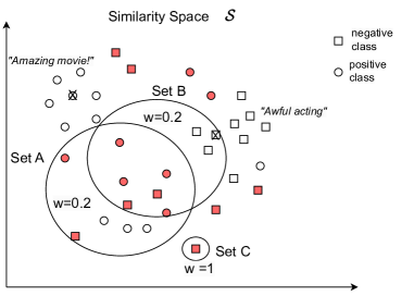
Figure 9: A beneficial case for AdaIcl+.

We provide an example of AdaIcl+’s advantage in Figure 9. In this example, AdaIcl+’s re-weighting schema scores Sets A and B higher than Set C, which contains only a single hard example. On the contrary, if Set A is selected by AdaIcl, all the examples of Set B would be marked as covered resulting in a zero total score. The next best scoring set would be Set C, which does not effectively represent the hardness of the examples. In AdaIcl+, Set B is scored higher than Set C due to its new weight $w=0.2$.

A.3 Set Construction

In this work, we represent the region $S_{i}$ around each example $x_{i}$ as its egonet. Initially, we build a global graph ${\mathcal{G}}_{m}$ as the $m$-nearest neighbors graph. The nearest neighbors are obtained with similarity metrics based on the space ${\mathcal{S}}$, i.e., via cosine similarity. For example, we can have the following edge sets for two nodes $v_{1}$ and $v_{2}$ with $m=4$: $\{v_{1}\xrightarrow[]{}v_{2},\;v_{1}\xrightarrow[]{}v_{3},\;v_{1}\xrightarrow[]{}v_{4},\;v_{1}\xrightarrow[]{}v_{5}\},\text{ and }\{v_{2}\xrightarrow[]{}v_{3},\;v_{2}\xrightarrow[]{}v_{6},\;v_{2}\xrightarrow[]{}v_{7},\;v_{2}\xrightarrow[]{}v_{1}\}.$

Deriving sets $S_{i}$ from the global graph ${\mathcal{G}}_{m}$ depends on the LLM’s feedback as we are interested in hard examples $x_{i}\in{\mathcal{U}}_{h}$ for the model. Thus, we color each node as a hard or an easy node based on whether they belong to ${\mathcal{U}}_{h}$. For example, we can have ${\mathcal{U}}_{h}=\{v_{1},v_{2},v_{3},v_{4}\}$ and $\{v_{5},v_{6},v_{7}\}\notin U_{h}$ for the case above.

For every hard node $v\in{\mathcal{U}}_{h}$, we construct its 1-hop egonet. We consider edges that direct towards $v$ from other hard nodes $v^{\prime}\in{\mathcal{U}}_{h}$. This ensures that representative examples $x_{i}$, that are likely to be retrieved during ICL inference, have denser egonets. For example, if we have $v_{2}\xrightarrow[]{}v_{1},v_{3}\xrightarrow[]{}v_{1}$ (we exclude links from easy nodes, e.g., $v_{5}\xrightarrow[]{}v_{1}$), we obtain $S_{1}=\text{egonet}(v_{1})=\{v_{2},v_{3}\}$. Similarly, we obtain egonets for other nodes, e.g., $S_{2}=\text{egonet}(v_{2})=\{v_{1},v_{4}\}$, while some nodes might have empty egonets if only easy nodes directs towards them, e.g., $S_{3}=\text{egonet}(v_{3})=\emptyset$. We experiment with both 1-hop and 2-hop set constructions. In the latter case, each node $v$ is represented by its egonet along with union of the egonets of its neighbors, e.g., $S^{(2)}_{1}=\text{ego}(v_{1})\cup\{\text{ego}(v^{\prime}):v^{\prime}\in\text{ego}(v_{1})\}=\{v_{2},v_{3}\}\cup\text{ego}(v_{2})\cup\text{ego}(v_{3})=\{v_{2},v_{3},v_{4}\}.$

One hyperparameter that controls the quality of the generated egonets is $m$, which is used during the construction of graph ${\mathcal{G}}_{m}$. In order to determine $m$, we employ a heuristic rule based on the desired maximum iterations $\hat{T}$ until the budget $B$ is exhausted, as well as the minimum number of hard examples $N_{\hat{\theta}}$ to be covered at each iteration, where $N_{\hat{\theta}}=\lfloor\hat{\theta}N_{\theta}\rfloor$ and $\hat{\theta}\in[0,1]$ is a hyper-parameter with default value $\hat{\theta}=0.5$. Assuming the graph has reciprocal edges, each node has approximately $\theta m$ and $\theta^{2}m^{2}$ hard examples as neighbors for 1-hop and 2-hop sets, respectively. If at each iteration we annotate $\frac{B}{\hat{T}}$ examples, and we wish to cover at least $N_{\hat{\theta}}$ hard examples, we need to satisfy $N_{\hat{\theta}}\leq\frac{B}{\hat{T}}\theta m$ (for 1-hop sets) and $N_{\hat{\theta}}\leq\frac{B}{\hat{T}}\theta^{2}m^{2}$ (for 2-hop sets). Thus, the heuristic-based rule is given by

$$\begin{cases}\frac{\hat{T}N_{\hat{\theta}}}{\theta B}\leq m\leq\frac{\hat{T}N_{\theta}}{\theta B}&\text{for 1-hop sets},\\ \frac{\hat{T}N_{\hat{\theta}}}{\theta^{2}B}\leq m^{2}\leq\frac{\hat{T}N_{\theta}}{\theta^{2}B}&\text{for 2-hop sets},\end{cases}$$ (7)

which is adjustable to the portion of the examples that we account as hard ones (the right hand side is derived due to constraint of maximum iterations $\hat{T}$). Moreover, instead of having a $m$-nn graph ${\mathcal{G}}_{m}$, we experiment with a threshold-based $\delta$-graph ${\mathcal{G}}_{\delta}$, where we set the threshold accordingly.

Appendix B Experimental Setting Details

B.1 Datasets

We performed empirical evaluation with nine NLP datasets that cover well-studied tasks, such as topic classification (AGNews (Zhang et al., 2015), TREC (Hovy et al., 2001)), sentiment analysis (SST2 (Socher et al., 2013), Amazon (McAuley & Leskovec, 2013)), natural language inference (RTE (Bentivogli et al., 2009), MRPC (Dolan et al., 2004), MNLI (Williams et al., 2018)), text summarization (XSUM (Narayan et al., )) and math reasoning (GSM8K (Cobbe et al., 2021)). We provide examples of these datasets in Table 3, which we access via Hugging Face package (Lhoest et al., 2021).

Table 3: Dataset examples. $<S_{1}>$ denotes the input sequences.

Dataset	Task	Example $x$	Labels/Annotations $y$
AGNews	Topic Classification	$<S_{1}>$: “Amazon Updates Web Services Tools, Adds Alexa Access The Amazon Web Services (AWS) division of online retail giant Amazon.com yesterday released Amazon E-Commerce Service 4.0 and the beta version of Alexa Web Information Service.”	World, Sport, Business, Sci-Tech
TREC	Answer Type Classification	$<S_{1}>$: “What is the date of Boxing Day?”	Abbreviation, Entity, Description, Human, Location, Numeric
SST2	Sentiment Analysis	$<S_{1}>$: “covers this territory with wit and originality , suggesting that with his fourth feature”	Positive, Negative
Amazon	Sentiment Analysis	$<S_{1a}>$:“Very Not Worth Your Time”, $<S_{1b}>$:“The book was written very horribly. I would never in my life recommend such a book…”	Positive, Negative
RTE	Natural Language Inference	$<S_{1}>$:“In a bowl, whisk together the eggs and sugar until completely blended and frothy.”, $<S_{2}>$:“In a bowl, whisk together the egg, sugar and vanilla until light in color.”	Entailment, Not Entailment
MRPC	Paraphrase Detection	$<S_{1}>$:“He said the foodservice pie business doesn’t fit the company’s long-term growth strategy.”, $<S_{2}>$:“The foodservice pie business does not fit our long-term growth strategy.”	Equivalent, Not Equivalent
MNLI	Natural Language Inference	$<S_{1}>$:“The new rights are nice enough”, $<S_{2}>$: “Everyone really likes the newest benefits”	Entailment, Neutral, Contradiction
XSUM	Summarization	$<S_{1}>$:“The 3kg (6.6lb) dog is set to become part of a search-and-rescue team used for disasters such as earthquakes. Its small size means it will be able to squeeze into places too narrow for dogs such as German Shepherds. Chihuahuas, named after a Mexican state, are one of the the smallest breeds of dog. ”It’s quite rare for us to have a chihuahua work as a police dog (said a police spokeswoman in Nara, western Japan). We would like it to work hard by taking advantage of its small size. Momo, aged seven, will begin work in January.”	“A chihuahua named Momo (Peach) has passed the exam to become a dog in the police force in western Japan, in what seems to be a first.”
GSM8K	Math Reasoning	$<S_{1}>$:“James writes a 3-page letter to 2 different friends twice a week. How many pages does he write a year?”	“He writes each friend 3*2=6 pages a week So he writes 6*2=12 pages every week That means he writes 12*52=624 pages a year. Thus, the answer is 624.”

Each dataset contains official train/dev/test splits. We follow Vote$k$ and sample 256 examples randomly from the test set (if it is publicly available, otherwise from the dev set) as test data. For the train data, we remove the annotations before our active learning setup. As it is infeasible to evaluate the LLM’s feedback on all instances due to computational constraints, e.g., Amazon dataset has more than 1 million instances, we randomly subsample 3,000 instances, which we cluster into 310 groups, and we select the 310 examples closest to the centroids as candidate examples for annotation. We repeat the above processes for both the train and test sets three times with different seeds and report mean and standard deviation results. In transductive settings, we only consider the test data for annotation. In this case, we evaluate performance on all test examples, but we also exclude retrieving examples that lead to self-label leakage issues.

B.2 Prompts

As a design choice of the input prompts, we slightly modify the templates proposed by Gao et al. (2021) to transform them as a continuation task. We find that these are more challenging prompts for the large LMs, which we present in Table 4 (top). In Section C.3, we also experiment with alternative prompt templates similar to Su et al. (2022), as shown in Table 4 (bottom).

Table 4: Prompt templates for the ICL demonstrations.

Task	Template	Continuation (label word)
	Default
AGNews	Content: $<S_{1}>\backslash n$	World, Sport, Business, Sci-Tech
TREC	Content: $<S_{1}>\backslash n$	Abbreviation, Entity, Description, Human, Location, Numeric
SST2	$<S_{1}>$. It was	great, terrible
Amazon	$<S_{1a}><S_{1b}>$. It was	great, terrible
RTE	$<S_{1}>$? [MASK], $<S_{2}>$	[MASK]: Yes, [MASK]: No
MRPC	$<S_{1}>$? [MASK], $<S_{2}>$	[MASK]: Yes, [MASK]: No
MNLI	$<S_{1}>$? [MASK], $<S_{2}>$	[MASK]: Yes, [MASK]: Maybe, [MASK]: No
	Alternative
AGNews	Content: $<S_{1}>$ Topic:	World, Sport, Business, Sci-Tech
TREC	Content: $<S_{1}>$ Answer Type:	Abbreviation, Entity, Description, Human, Location, Numeric
SST2	Content: $<S_{1}>$ Sentiment:	Positive, Negative
Amazon	Title: $<S_{1a}>$ Review: $<S_{1b}>$ Sentiment:	Positive, Negative
RTE	$<S_{1}>$. Question: $<S_{2}>$. True or False? Answer:	True, False
MRPC	Are the following sentences equivalent or not equivalent? $<S_{1}>\backslash n<S_{2}>$	equivalent, not equivalent
MNLI	$<S_{1}>$. Based on that information, is the claim $<S_{2}>$ True, False, or Inconclusive? Answer:	True, Inconclusive, False

B.3 Configurations

As summarized in Figure 2, the design space includes the unlabeled set ${\mathcal{U}}$, the number of ICL examples $k$, the similarity space ${\mathcal{S}}$, the budget $B$, and the LLM $M$. We use the default hyper-parameters of the Transformers library (Wolf et al., 2020) for each LLM. We obtain the initial pool of annotated examples ${\mathcal{L}}_{0}$ via $k$means so that we reduce randomness. We summarize the experimental configurations in Table 5.

Table 5: Experimental setting configurations.

Setting	Models $M$	Train/Test ${\mathcal{U}}$	Budget $B$	$k$-shot	Retriever, ${\mathcal{S}}$	Init.
Main
Figure 4	GPTJ, GPT-Neo	Inductive	20	5	SBERT	$|{\mathcal{L}}_{0}|=10$
XSUM	Falcon-40B, LLaMa-65B	Transductive	10	Context-limit	SBERT	Zero-shot
GSM8K	Falcon-40B, LLaMa-65B	Transductive	20	5	BERT,SBERT	Zero-shot
Table 1	GPT-J, MPT	Transductive	5,10	5,10	SBERT	Zero-shot
Table 2	GPT-Neo	Inductive	20	5	SBERT, RoBERTa, BERT	$|{\mathcal{L}}_{0}|=10$
Figure 5	GPT-Neo	Transductive	0-45	Context-limit	SBERT	Zero-shot
Figure 6	GPT-J, MPT, Falcon, LLaMa (6-7B)	Transductive	0-20	Context-limit	SBERT	Zero-shot
Figure 7	GPT-Neo	Transductive	0-45	Context-limit	SBERT	Zero-shot
Appendices C, D	GPT-J, GPT-Neo	Inductive	20	5	SBERT	$|{\mathcal{L}}_{0}|=10$

• Context-limit means that we retrieve as many few-shot examples as the input token-length limit allows. For example, XSUM has long sequences, where we usually have 3-shot examples, while for TREC we can use as many as 80-shot examples.

Appendix C Further Results

C.1 Base Results (Full)

Tables 6 and  7 give the full results of Figure 4 for GPT-J and GPT-Neo, accordingly. AdaIcl performs the best over all tasks, while the second-best method is AdaIcl-base.

Table 6: Performance comparison for GPT-J (6B).

	Topic Classification		Sentiment Analysis		Natural Language Inference
	AGNews	TREC	SST2	Amazon	RTE	MRPC	MNLI
Random	$68.87_{\pm 5.39}$	$49.34_{\pm 3.19}$	$81.63_{\pm 0.30}$	$87.89_{\pm 1.77}$	$52.86_{\pm 2.41}$	$69.01_{\pm 4.61}$	$39.58_{\pm 3.98}$
Fast-vote$k$	$73.69_{\pm 2.39}$	$49.61_{\pm 4.43}$	$78.99_{\pm 4.53}$	$89.58_{\pm 0.80}$	$53.00_{\pm 0.49}$	$68.23_{\pm 2.89}$	$39.97_{\pm 3.98}$
Vote$k$	$72.26_{\pm 1.27}$	$45.83_{\pm 1.75}$	$80.45_{\pm 1.47}$	$85.80_{\pm 3.80}$	$54.16_{\pm 2.30}$	$68.10_{\pm 2.75}$	$39.72_{\pm 2.07}$
Hardest	$72.13_{\pm 2.12}$	$35.93_{\pm 5.53}$	$82.67_{\pm 1.64}$	$87.36_{\pm 0.66}$	$55.33_{\pm 2.25}$	$66.80_{\pm 5.25}$	$38.80_{\pm 1.11}$
AdaIcl-base	$73.56_{\pm 2.96}$	$50.64_{\pm 9.11}$	$84.11_{\pm 3.25}$	$91.01_{\pm 1.77}$	$52.73_{\pm 2.21}$	$66.53_{\pm 4.78}$	$38.66_{\pm 4.50}$
Best (Avg.)	AdaIcl-base ($62.10$)		AdaIcl-base ($87.56$)		Vote$k$ ($53.99$)
AdaIcl	$76.89_{\pm 3.01}$	$51.95_{\pm 8.43}$	$82.81_{\pm 1.39}$	$90.49_{\pm 1.57}$	$56.90_{\pm 1.75}$	$70.17_{\pm 1.72}$	$40.36_{\pm 1.75}$
AdaIcl+	$77.08_{\pm 1.11}$	$53.38_{\pm 5.10}$	$84.24_{\pm 1.32}$	$92.45_{\pm 1.50}$	$55.07_{\pm 0.85}$	$68.49_{\pm 0.97}$	$36.58_{\pm 1.12}$
Best (Avg.)	AdaIcl+ ($65.23$)		AdaIcl+ ($88.35$)		AdaIcl ($55.81$)
$\Delta$-Gain (Absolute)	$+3.13$		$+0.79$		$+1.82$

Table 7: Performance comparison for GPT-Neo (1.3B).

	Topic Classification		Sentiment Analysis		Natural Language Inference
	AGNews	TREC	SST2	Amazon	RTE	MRPC	MNLI
Random	$59.47_{\pm 8.54}$	$54.68_{\pm 1.68}$	$68.48_{\pm 1.87}$	$73.95_{\pm 2.03}$	$48.30_{\pm 1.30}$	$64.48_{\pm 7.67}$	$40.99_{\pm 0.97}$
Fast-vote$k$	$62.23_{\pm 3.89}$	$46.48_{\pm 3.04}$	$69.78_{\pm 8.34}$	$69.39_{\pm 0.98}$	$50.64_{\pm 1.02}$	$64.19_{\pm 0.97}$	$38.40_{\pm 0.92}$
Vote$k$	$62.77_{\pm 4.82}$	$53.12_{\pm 4.07}$	$73.69_{\pm 9.05}$	$75.13_{\pm 0.98}$	$49.99_{\pm 0.32}$	$67.44_{\pm 2.96}$	$39.18_{\pm 1.60}$
Hardest	$65.10_{\pm 2.43}$	$49.34_{\pm 2.17}$	$71.48_{\pm 5.32}$	$75.00_{\pm 2.49}$	$52.86_{\pm 0.80}$	$61.84_{\pm 4.79}$	$37.49_{\pm 1.77}$
AdaIcl-base	$70.17_{\pm 1.84}$	$48.24_{\pm 0.98}$	$77.86_{\pm 1.02}$	$75.77_{\pm 3.62}$	$53.77_{\pm 0.73}$	$64.71_{\pm 7.39}$	$39.71_{\pm 1.03}$
Best (Avg.)	AdaIcl-base ($59.21$)		AdaIcl-base ($76.82$)		Vote$k$ ($52.20$)
AdaIcl	$70.95_{\pm 1.87}$	$55.33_{\pm 2.57}$	$79.68_{\pm 1.77}$	$77.73_{\pm 2.23}$	$53.12_{\pm 1.59}$	$67.05_{\pm 8.10}$	$42.96_{\pm 2.92}$
AdaIcl+	$69.39_{\pm 1.35}$	$59.89_{\pm 2.07}$	$79.03_{\pm 2.47}$	$77.08_{\pm 1.50}$	$51.16_{\pm 1.39}$	$65.69_{\pm 8.92}$	$40.49_{\pm 2.04}$
Best (Avg.)	AdaIcl+ ($64.64$)		AdaIcl ($78.71$)		AdaIcl ($54.38$)
$\Delta$-Gain (Absolute)	$+5.53$		$+1.99$		$+2.28$

C.2 Retriever Ablation

Table 8: Performance comparison across different retrieval and semantic similarity configurations.

Retriever, ${\mathcal{S}}\xrightarrow{}$	SBERT-all-mpnet-base			RoBERTa-nli-large-mean-tokens			BERT-nli-large-cls-pool			Avg.
	TREC	SST2	Amazon	TREC	SST2	Amazon	TREC	SST2	Amazon
Random	$54.68_{\pm 1.68}$	$68.48_{\pm 1.87}$	$73.95_{\pm 2.03}$	$37.23_{\pm 2.30}$	$74.21_{\pm 3.50}$	$84.46_{\pm 3.21}$	$34.75_{\pm 2.41}$	$72.65_{\pm 5.82}$	$80.20_{\pm 3.34}$	$64.51$
Vote$k$	$54.81_{\pm 0.49}$	$73.69_{\pm 9.05}$	$75.13_{\pm 0.98}$	$37.77_{\pm 4.65}$	$76.16_{\pm 2.23}$	$84.11_{\pm 1.28}$	$42.43_{\pm 3.34}$	$80.85_{\pm 2.09}$	$83.59_{\pm 1.77}$	$67.61$
AdaIcl-base	$48.24_{\pm 0.98}$	$77.86_{\pm 1.02}$	$75.77_{\pm 3.63}$	$38.12_{\pm 5.74}$	$78.12_{\pm 5.30}$	$\underline{85.93}_{\pm 2.30}$	$38.15_{\pm 3.10}$	$78.64_{\pm 2.78}$	$\underline{85.80}_{\pm 1.75}$	$67.40$
AdaIcl	$\underline{55.33}_{\pm 2.57}$	$\underline{79.68}_{\pm 2.47}$	$\underline{77.73}_{\pm 2.23}$	$\underline{39.06}_{\pm 3.37}$	$\underline{81.11}_{\pm 1.50}$	$85.15_{\pm 0.55}$	$44.06_{\pm 2.49}$	$\underline{80.85}_{\pm 2.83}$	$84.65_{\pm 3.52}$	69.74
random reorder
Random	$47.39_{\pm 2.89}$	$66.57_{\pm 3.86}$	$76.42_{\pm 2.57}$	$31.87_{\pm 4.45}$	$69.74_{\pm 5.84}$	$81.24_{\pm 2.72}$	$40.34_{\pm 1.58}$	$76.55_{\pm 4.06}$	$79.54_{\pm 2.64}$	$63.29$
Vote$k$	$45.43_{\pm 2.94}$	$72.00_{\pm 3.73}$	$73.04_{\pm 1.77}$	$37.62_{\pm 5.15}$	$75.91_{\pm 5.58}$	$82.03_{\pm 0.84}$	$39.57_{\pm 3.19}$	$79.29_{\pm 2.55}$	$81.24_{\pm 1.43}$	$65.13$
AdaIcl-base	$50.64_{\pm 5.43}$	$74.99_{\pm 6.37}$	$74.86_{\pm 4.65}$	$36.56_{\pm 2.98}$	$75.77_{\pm 0.63}$	$84.89_{\pm 2.02}$	$\underline{45.56}_{\pm 3.01}$	$79.55_{\pm 0.18}$	$85.41_{\pm 0.91}$	$67.58$
AdaIcl	$52.22_{\pm 5.19}$	$78.12_{\pm 4.71}$	$75.64_{\pm 3.51}$	$38.93_{\pm 0.48}$	$76.68_{\pm 2.71}$	$84.11_{\pm 1.43}$	$44.00_{\pm 1.63}$	$78.51_{\pm 4.52}$	$85.28_{\pm 4.65}$	68.16

A benefit of the $k$-NN retriever is that it can determine the order of the input few-shot examples by semantic similarity scores. In general, we place demonstrations with higher similarity closer to the test instance. Table 8 gathers results for different retrievers as well as when we randomly re-order the input demonstrations. AdaIcl is the most robust method and outperforms other baselines regardless of the choice of the retriever.

C.3 Prompt Template Ablation

Table 9: Prompt template ablation study.

	GPT-Neo				GPT-J
	AGNews	TREC	SST2	Amazon	RTE	MRPC	MNLI
	Default Prompts
Random	$59.47_{\pm 8.54}$	$54.68_{\pm 1.68}$	$68.48_{\pm 1.87}$	$73.95_{\pm 2.03}$	$52.86_{\pm 2.41}$	$69.01_{\pm 4.61}$	$39.58_{\pm 3.98}$
Vote$k$	$62.77_{\pm 4.82}$	$53.12_{\pm 4.07}$	$73.69_{\pm 9.05}$	$75.13_{\pm 0.98}$	$54.16_{\pm 2.30}$	$68.10_{\pm 2.75}$	$39.72_{\pm 2.07}$
AdaIcl	$70.95_{\pm 1.87}$	$55.33_{\pm 2.57}$	$79.68_{\pm 1.77}$	$77.73_{\pm 2.23}$	$56.90_{\pm 1.75}$	$70.17_{\pm 1.72}$	$40.36_{\pm 1.75}$
	Alternative Prompts
Random	$73.69_{\pm 1.21}$	$51.76_{\pm 4.55}$	$59.89_{\pm 3.98}$	$73.82_{\pm 3.35}$	$56.41_{\pm 2.13}$	$56.37_{\pm 3.72}$	$38.93_{\pm 1.18}$
Vote$k$	$72.78_{\pm 2.12}$	$50.38_{\pm 5.90}$	$64.84_{\pm 2.92}$	$73.43_{\pm 2.23}$	$56.38_{\pm 2.70}$	$51.95_{\pm 2.53}$	$40.49_{\pm 2.05}$
AdaIcl	$76.95_{\pm 1.27}$	$54.94_{\pm 1.43}$	$65.88_{\pm 4.58}$	$75.64_{\pm 1.29}$	$56.37_{\pm 1.29}$	$59.22_{\pm 2.39}$	$35.40_{\pm 1.31}$

Table 9 reports results when we use alternative ICL prompt templates (Table 4) for the input examples. AdaIcl is robust to the design of the prompt templates, where it outperforms other baselines in most datasets.

C.4 Calibration Analysis via Simplices

Calibration has recently also been studied from the perspective of simplices (Heese et al., 2023). Abstractly, a simplex is the generalization of the notion of a triangle/ tetrahedron to arbitrary dimensions. Here, we present a simplified study of calibration via the lens of simplices, where we test if the predicted label of the test instance lies within the simplex given by the retrieved examples having the same label. In more detail, given a prediction $y_{test}=\bm{y}$ for test instance $x_{test}$, we first obtain the subset of retrieved examples for $x_{test}$, i.e. ${\mathcal{X}}_{subset}\subseteq{\mathcal{X}}_{retrieved}\subset B$ which share the same label $\bm{y}$. We then construct a simplex using the SBERT embeddings of ${\mathcal{X}}_{subset}$, run PCA to obtain low dimensional embeddings and test to see if the low dimensional embedding of $x_{test}$ lies within the above constructed simplex.

To take into consideration the effect of overconfident but wrong predictions, for a given dataset, we subtract the total counts of the cases when $\bm{y}\not=\bm{y}_{true}$ from the cases where $\bm{y}=\bm{y}_{true}$ for all $x_{test}$ in the dataset. Results are presented in the plots in Figure 10 where we compare AdaIcl against random and the best performing baseline on that dataset. For AGNews, TREC, and SST2, the label information of the retrieved examples is important and AdaIcl leads to the best calibration in these cases. For RTE, MRPC, and MNLI, retrieving examples of the same label is not crucial for performance and thus, all methods behave similarly with respect to simplex calibration.

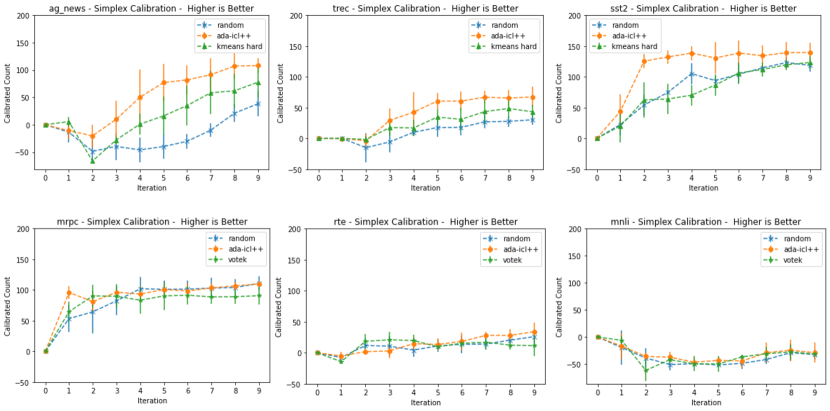
Figure 10: Calibration analysis via simplicies where we compare AdaIcl against the random selection algorithm and the best performing baseline for each dataset.

C.5 Selection Time Complexity

In Table 10, we compare competing approaches based on their computation time during their selection process (during downstream inference, their time complexity is the same). Random selection has zero cost. Vote$k$ and AdaIcl ($T=1$) have the same cost, while the cost doubles for AdaIcl ($T=2$). Nevertheless, hyper-parameter $T$ for AdaIcl can be tuned depending on the desired runtime of the selection process.

Table 10: Time complexity analysis with 5-shot ICL for different selection processes over 300 examples on a GeForce RTX 3090 (24GB GPU).

	Embedding Computation (SBERT)	Model Uncertainty Estimation (GPT-Neo)
Amazon
Random	0 secs	0 secs
Vote$k$	$\approx$1 secs	1 min & 51 secs
AdaIcl ($T=1$)	$\approx$1 secs	1 min & 51 secs
AdaIcl ($T=2$)	$\approx$1 secs	$\approx$ 3 mins & 42 secs
AGNews
Random	0 secs	0 secs
Vote$k$	$\approx$0.5 secs	3 mins & 48 secs
AdaIcl ($T=1$)	$\approx$0.5 secs	3 mins & 48 secs
AdaIcl ($T=2$)	$\approx$0.5 secs	$\approx$ 7 mins & 36 secs

Appendix D AdaIcl Ablation Studies

D.1 Graph Ablation Studies

Table 11: Graph ablation study using GPT-Neo based on hyper-parameters $m$, which controls the number of graph neighbors, and $l$, which controls whether we consider 1-hop or 2-hop sets. The value combinations of $m$ and $l$ are adjusted via Equation 7.

	AGNews	SST2	Amazon
Vote$k$	$62.77_{\pm 4.82}$	$73.69_{\pm 9.05}$	$75.13_{\pm 0.98}$
AdaIcl
$m=15,l=1$	$68.61_{\pm 1.02}$	$79.42_{\pm 1.28}$	$77.34_{\pm 2.73}$
$m=25,l=1$	$68.74_{\pm 3.59}$	$77.60_{\pm 4.20}$	$76.95_{\pm 3.86}$
$m=5,l=2$	$70.95_{\pm 1.87}$	$79.68_{\pm 1.77}$	$77.73_{\pm 2.23}$
$m=7,l=2$	$69.13_{\pm 1.39}$	$78.12_{\pm 2.61}$	$74.99_{\pm 0.84}$
AdaIcl+ ($T=2$)
$m=15,l=1$	$69.39_{\pm 1.35}$	$79.03_{\pm 2.47}$	$77.08_{\pm 1.50}$
$m=25,l=1$	$68.87_{\pm 3.26}$	$77.73_{\pm 2.22}$	$73.17_{\pm 2.59}$
$m=5,l=2$	$70.43_{\pm 1.60}$	$77.73_{\pm 1.15}$	$76.43_{\pm 2.55}$
$m=7,l=2$	$70.60_{\pm 2.89}$	$76.95_{\pm 4.69}$	$77.21_{\pm 2.12}$

• *Denotes the default value.

Table 11 shows an ablation study on our proposed heuristic rule of Equation 7. We select $m$ such that it lies near the boundaries of  Equation 7, depending whether we choose $l=1$ hop sets or $l=2$ hop sets. As Table 11 shows, our heuristic rule is robust and achieves good results with four different combinations. In some cases, having smaller values of $m$ leads to slightly better results as it excludes neighbors with less semantic similarity.

Table 12: Graph ablation study for AdaIcl using GPT-J with different graph construction approaches.

	AGNews	TREC	SST2	Amazon	RTE	MRPC	MNLI
$m$-nn graph	$77.08_{\pm 1.11}$	$53.38_{\pm 5.10}$	$84.24_{\pm 1.32}$	$92.45_{\pm 1.50}$	$56.90_{\pm 1.75}$	$70.17_{\pm 1.72}$	$40.36_{\pm 1.75}$
$\delta$-graph	$76.17_{\pm 3.45}$	$50.51_{\pm 4.65}$	$81.90_{\pm 2.48}$	$88.80_{\pm 1.57}$	$56.63_{\pm 3.23}$	$68.75_{\pm 1.93}$	$40.62_{\pm 2.08}$

Furthermore, we also experiment with using a threshold-based graph ($\delta$-graph) instead of the $m$-nn graph. To determine threshold $\delta$, we compute the cosine similarity between all nodes and set $\delta$ such as each node has $m$ neighbors on average (at the $m$-nn graph each nodes has exactly $m$ neighbors). As Table 12 shows, using the $\delta$-graph performs slightly worse than the $m$-nn graph. We hypothesize that using the $\delta$-graph gives more importance on the semantics of the train distribution (as $\delta$ value is computed based on the similarity scores between all train examples), which may not always generalize well to the test distribution.

D.2 Uncertainty Threshold

Table 13: Ablation study using GPT-Neo based on hyper-parameter $\theta$, which controls the number of the examples that are considered as hard ones.

	TREC	SST2	Amazon
Vote$k$	$53.12_{\pm 4.07}$	$73.69_{\pm 9.05}$	$75.13_{\pm 0.98}$
AdaIcl+ ($\theta=0.5$)	$59.89_{\pm 2.07}$	$79.03_{\pm 2.47}$	$77.08_{\pm 1.50}$
AdaIcl+ ($\theta=0.33$)	$60.28_{\pm 3.13}$	$78.77_{\pm 2.59}$	$78.90_{\pm 1.14}$

By default, we consider 50% ($\theta=0.5$) of the examples with the lowest confidence as hard examples. Table 13 shows results when we focus on harder examples by setting $\theta=0.33$ for AdaIcl+. Interestingly, AdaIcl+’s performance can be further boosted with careful tuning of the uncertainty threshold. Thus, automatically determining which examples are considered as hard examples for the models seems a promising research direction.

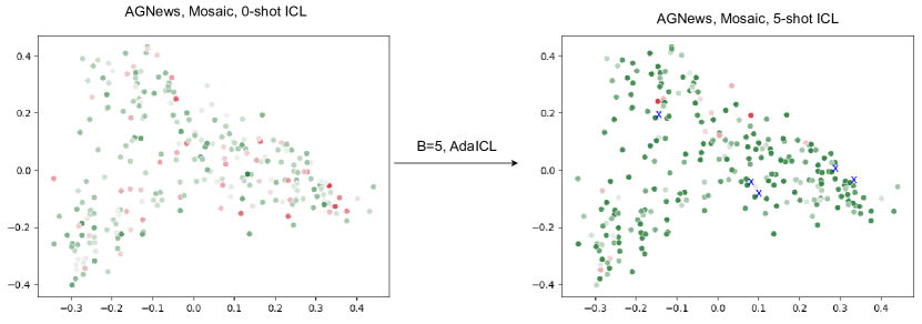
(a) 5-shot ICL by AdaIcl selection for AGNews with Mosaic.

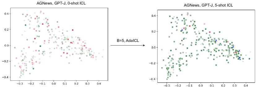
(b) 5-shot ICL by AdaIcl selection for AGNews with GPT-J.

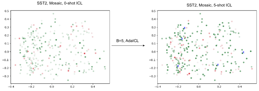
(c) 5-shot ICL by AdaIcl selection for SST2 with Mosaic.

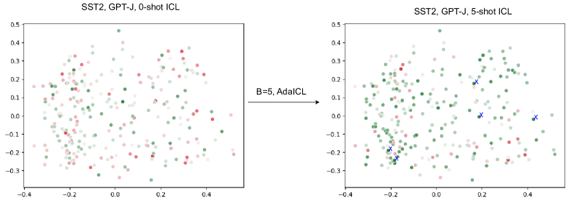
(d) 5-shot ICL by AdaIcl selection for SST2 with GPT-J.

Figure 11: Visualization of the SBERT space (after PCA) and of the examples selected for annotation. The two axes represent the two most important PCA components, which is performed over the SBERT embeddings of the examples. The hue color (green to red) represents the model’s uncertainty (confident to uncertain) for each example. The selected examples for annotation are marked with the blue ‘X’ symbol (better viewed with zooming).

Appendix E Visualization

We illustrate the selection process of AdaIcl in Figure 11. Initially, the LLMs perform 0-shot ICL but do not make confident predictions (as the hue color, that represents the model’s uncertainty for each example, indicates). Note that different LLMs may consider different examples as hard or easy ones. Then, AdaIcl selects 5 representative for 5-shot ICL, which improves the LLMs’ understanding of the task and reduces its uncertainty (we observe fewer red nodes and more nodes with greener color).

Appendix F AdaIcl Limitations

We list some of our assumptions that may limit AdaIcl if they are not satisfied. First, we assume that we can access the output logits/probabilities from the LLM in order to evaluate its uncertainty; this might not be always be feasible. Second, AdaIcl relies on embedding methods to determine semantic diversity. While AdaIcl is shown to be robust to different methods, it can still suffer if the semantic space of the test is wildly different from the annotation pool space. Finally, the graph/set construction is a heuristic approach and does not account for cases where adversarial examples are injected into the pool in order to degrade performance.

References

- Akyürek et al. (2023) Ekin Akyürek, Dale Schuurmans, Jacob Andreas, Tengyu Ma, and Denny Zhou. What learning algorithm is in-context learning? investigations with linear models. ICLR, 2023.
- Bai et al. (2023) Yu Bai, Fan Chen, Huan Wang, Caiming Xiong, and Song Mei. Transformers as statisticians: Provable in-context learning with in-context algorithm selection. arXiv preprint arXiv:2306.04637, 2023.
- Bansal et al. (2023) Hritik Bansal, Karthik Gopalakrishnan, Saket Dingliwal, Sravan Bodapati, Katrin Kirchhoff, and Dan Roth. Rethinking the role of scale for in-context learning: An interpretability-based case study at 66 billion scale. ACL, 2023.
- Bentivogli et al. (2009) Luisa Bentivogli, Peter Clark, Ido Dagan, and Danilo Giampiccolo. The fifth pascal recognizing textual entailment challenge. TAC, 2009.
- Bommasani et al. (2021) Rishi Bommasani, Drew A Hudson, Ehsan Adeli, Russ Altman, Simran Arora, Sydney von Arx, Michael S Bernstein, Jeannette Bohg, Antoine Bosselut, Emma Brunskill, et al. On the opportunities and risks of foundation models. arXiv preprint arXiv:2108.07258, 2021.
- Brown et al. (2020) Tom Brown, Benjamin Mann, Nick Ryder, Melanie Subbiah, Jared D Kaplan, Prafulla Dhariwal, Arvind Neelakantan, Pranav Shyam, Girish Sastry, Amanda Askell, et al. Language models are few-shot learners. NeurIPS, 2020.
- Chan et al. (2022) Stephanie Chan, Adam Santoro, Andrew Lampinen, Jane Wang, Aaditya Singh, Pierre Richemond, James McClelland, and Felix Hill. Data distributional properties drive emergent in-context learning in transformers. NeurIPS, 2022.
- Chen et al. (2022a) Yanda Chen, Chen Zhao, Zhou Yu, Kathleen McKeown, and He He. On the relation between sensitivity and accuracy in in-context learning. arXiv preprint arXiv:2209.07661, 2022a.
- Chen et al. (2022b) Yanda Chen, Ruiqi Zhong, Sheng Zha, George Karypis, and He He. Meta-learning via language model in-context tuning. ACL, 2022b.
- Cobbe et al. (2021) Karl Cobbe, Vineet Kosaraju, Mohammad Bavarian, Mark Chen, Heewoo Jun, Lukasz Kaiser, Matthias Plappert, Jerry Tworek, Jacob Hilton, Reiichiro Nakano, et al. Training verifiers to solve math word problems. arXiv preprint arXiv:2110.14168, 2021.
- Devlin et al. (2019) Jacob Devlin, Ming-Wei Chang, Kenton Lee, and Kristina Toutanova. Bert: Pre-training of deep bidirectional transformers for language understanding. In NAACL, 2019.
- Diao et al. (2023) Shizhe Diao, Pengcheng Wang, Yong Lin, and Tong Zhang. Active prompting with chain-of-thought for large language models. arXiv preprint arXiv:2302.12246, 2023.
- Dolan et al. (2004) Bill Dolan, Chris Quirk, and Chris Brockett. Unsupervised construction of large paraphrase corpora: Exploiting massively parallel news sources. In COLING 2004: Proceedings of the 20th International Conference on Computational Linguistics, aug 23–aug 27 2004. URL https://aclanthology.org/C04-1051.
- Dong et al. (2022) Qingxiu Dong, Lei Li, Damai Dai, Ce Zheng, Zhiyong Wu, Baobao Chang, Xu Sun, Jingjing Xu, and Zhifang Sui. A survey for in-context learning. arXiv preprint arXiv:2301.00234, 2022.
- Ein-Dor et al. (2020) Liat Ein-Dor, Alon Halfon, Ariel Gera, Eyal Shnarch, Lena Dankin, Leshem Choshen, Marina Danilevsky, Ranit Aharonov, Yoav Katz, and Noam Slonim. Active Learning for BERT: An Empirical Study. In EMNLP, 2020.
- Erdmann et al. (2019) Alexander Erdmann, David Joseph Wrisley, Benjamin Allen, Christopher Brown, Sophie Cohen-Bodénès, Micha Elsner, Yukun Feng, Brian Joseph, Béatrice Joyeux-Prunel, and Marie-Catherine de Marneffe. Practical, efficient, and customizable active learning for named entity recognition in the digital humanities. In EMNLP, 2019.
- Gao et al. (2021) Tianyu Gao, Adam Fisch, and Danqi Chen. Making pre-trained language models better few-shot learners. In ACL, 2021.
- Garg et al. (2022) Shivam Garg, Dimitris Tsipras, Percy S Liang, and Gregory Valiant. What can transformers learn in-context? a case study of simple function classes. NeurIPS, 2022.
- Guo et al. (2017) Chuan Guo, Geoff Pleiss, Yu Sun, and Kilian Q Weinberger. On calibration of modern neural networks. In ICML, 2017.
- Haffari et al. (2009) Gholamreza Haffari, Maxim Roy, and Anoop Sarkar. Active learning for statistical phrase-based machine translation. In NAACL, 2009.
- Hahn & Goyal (2023) Michael Hahn and Navin Goyal. A theory of emergent in-context learning as implicit structure induction. arXiv preprint arXiv:2303.07971, 2023.
- Han et al. (2023) Chi Han, Ziqi Wang, Han Zhao, and Heng Ji. In-context learning of large language models explained as kernel regression. arXiv preprint arXiv:2305.12766, 2023.
- Heese et al. (2023) Raoul Heese, Jochen Schmid, Michał Walczak, and Michael Bortz. Calibrated simplex-mapping classification. PLoS One, 18(1):e0279876, 2023.
- Hovy et al. (2001) Eduard Hovy, Laurie Gerber, Ulf Hermjakob, Chin-Yew Lin, and Deepak Ravichandran. Toward semantics-based answer pinpointing. In Proceedings of the First International Conference on Human Language Technology Research, 2001. URL https://www.aclweb.org/anthology/H01-1069.
- Jiang et al. (2021) Zhengbao Jiang, Jun Araki, Haibo Ding, and Graham Neubig. How can we know when language models know? on the calibration of language models for question answering. Transactions of the Association for Computational Linguistics, 9:962–977, 2021.
- Krause & Guestrin (2005) Andreas Krause and Carlos Guestrin. A note on the budgeted maximization of submodular functions. Citeseer, 2005.
- Lewis & Gale (1994) David D. Lewis and William A. Gale. A sequential algorithm for training text classifiers. SIGIR, 1994.
- Lhoest et al. (2021) Quentin Lhoest, Albert Villanova del Moral, Yacine Jernite, Abhishek Thakur, Patrick von Platen, Suraj Patil, Julien Chaumond, Mariama Drame, Julien Plu, Lewis Tunstall, Joe Davison, Mario Šaško, Gunjan Chhablani, Bhavitvya Malik, Simon Brandeis, Teven Le Scao, Victor Sanh, Canwen Xu, Nicolas Patry, Angelina McMillan-Major, Philipp Schmid, Sylvain Gugger, Clément Delangue, Théo Matussière, Lysandre Debut, Stas Bekman, Pierric Cistac, Thibault Goehringer, Victor Mustar, François Lagunas, Alexander Rush, and Thomas Wolf. Datasets: A community library for natural language processing. In Proceedings of the 2021 Conference on Empirical Methods in Natural Language Processing: System Demonstrations, 2021.
- Li & Qiu (2023) Xiaonan Li and Xipeng Qiu. Finding supporting examples for in-context learning. arXiv preprint arXiv:2302.13539, 2023.
- Liu et al. (2021) Jiachang Liu, Dinghan Shen, Yizhe Zhang, Bill Dolan, Lawrence Carin, and Weizhu Chen. What makes good in-context examples for gpt-? arXiv preprint arXiv:2101.06804, 2021.
- Liu et al. (2019) Yinhan Liu, Myle Ott, Naman Goyal, Jingfei Du, Mandar Joshi, Danqi Chen, Omer Levy, Mike Lewis, Luke Zettlemoyer, and Veselin Stoyanov. Roberta: A robustly optimized bert pretraining approach. arXiv preprint arXiv:1907.11692, 2019.
- Lu et al. (2022) Yao Lu, Max Bartolo, Alastair Moore, Sebastian Riedel, and Pontus Stenetorp. Fantastically ordered prompts and where to find them: Overcoming few-shot prompt order sensitivity. ACL, 2022.
- Ma et al. (2023) Huan Ma, Changqing Zhang, Yatao Bian, Lemao Liu, Zhirui Zhang, Peilin Zhao, Shu Zhang, Huazhu Fu, Qinghua Hu, and Bingzhe Wu. Fairness-guided few-shot prompting for large language models. arXiv preprint arXiv:2303.13217, 2023.
- MacQueen et al. (1967) James MacQueen et al. Some methods for classification and analysis of multivariate observations. In Proceedings of the fifth Berkeley symposium on mathematical statistics and probability, volume 1, pp. 281–297. Oakland, CA, USA, 1967.
- Margatina et al. (2021) Katerina Margatina, Giorgos Vernikos, Loïc Barrault, and Nikolaos Aletras. Active learning by acquiring contrastive examples. In EMNLP, 2021.
- Margatina et al. (2023) Katerina Margatina, Timo Schick, Nikolaos Aletras, and Jane Dwivedi-Yu. Active learning principles for in-context learning with large language models, 2023.
- McAuley & Leskovec (2013) Julian McAuley and Jure Leskovec. Hidden factors and hidden topics: Understanding rating dimensions with review text. In Proceedings of the 7th ACM Conference on Recommender Systems (RecSys), 2013. ISBN 9781450324090.
- Min et al. (2022a) Sewon Min, Mike Lewis, Luke Zettlemoyer, and Hannaneh Hajishirzi. Metaicl: Learning to learn in context. NAACL, 2022a.
- Min et al. (2022b) Sewon Min, Xinxi Lyu, Ari Holtzman, Mikel Artetxe, Mike Lewis, Hannaneh Hajishirzi, and Luke Zettlemoyer. Rethinking the role of demonstrations: What makes in-context learning work? EMNLP, 2022b.
- MosaicML (2023) MosaicML. Introducing mpt-7b: A new standard for open-source, commercially usable llms, 2023. URL www.mosaicml.com/blog/mpt-7b.
- (41) Shashi Narayan, Shay B. Cohen, and Mirella Lapata. Don’t give me the details, just the summary! topic-aware convolutional neural networks for extreme summarization. In Proceedings of the 2018 Conference on Empirical Methods in Natural Language Processing. URL https://aclanthology.org/D18-1206.
- Nguyen & Wong (2023) Tai Nguyen and Eric Wong. In-context example selection with influences. arXiv preprint arXiv:2302.11042, 2023.
- Olsson et al. (2022) Catherine Olsson, Nelson Elhage, Neel Nanda, Nicholas Joseph, Nova DasSarma, Tom Henighan, Ben Mann, Amanda Askell, Yuntao Bai, Anna Chen, et al. In-context learning and induction heads. arXiv preprint arXiv:2209.11895, 2022.
- Penedo et al. (2023) Guilherme Penedo, Quentin Malartic, Daniel Hesslow, Ruxandra Cojocaru, Alessandro Cappelli, Hamza Alobeidli, Baptiste Pannier, Ebtesam Almazrouei, and Julien Launay. The RefinedWeb dataset for Falcon LLM: outperforming curated corpora with web data, and web data only. arXiv preprint arXiv:2306.01116, 2023.
- Perez et al. (2021) Ethan Perez, Douwe Kiela, and Kyunghyun Cho. True few-shot learning with language models. NeurIPS, 2021.
- Pitis et al. (2023) Silviu Pitis, Michael R Zhang, Andrew Wang, and Jimmy Ba. Boosted prompt ensembles for large language models. arXiv preprint arXiv:2304.05970, 2023.
- Razeghi et al. (2022) Yasaman Razeghi, Robert L Logan IV, Matt Gardner, and Sameer Singh. Impact of pretraining term frequencies on few-shot numerical reasoning. EMNLP-Findings, 2022.
- Reimers & Gurevych (2019) Nils Reimers and Iryna Gurevych. Sentence-bert: Sentence embeddings using siamese bert-networks. EMNLP, 2019.
- Rubin et al. (2022) Ohad Rubin, Jonathan Herzig, and Jonathan Berant. Learning to retrieve prompts for in-context learning. NAACL, 2022.
- Schröder et al. (2022) Christopher Schröder, Andreas Niekler, and Martin Potthast. Revisiting uncertainty-based query strategies for active learning with transformers. ACL Findings, 2022.
- Schröder & Niekler (2020) Christopher Schröder and Andreas Niekler. A survey of active learning for text classification using deep neural networks, 2020.
- Sener & Savarese (2018) Ozan Sener and Silvio Savarese. Active learning for convolutional neural networks: A core-set approach. ICLR, 2018.
- Settles (2009) Burr Settles. Active learning literature survey. 2009.
- Shin et al. (2022) Seongjin Shin, Sang-Woo Lee, Hwijeen Ahn, Sungdong Kim, HyoungSeok Kim, Boseop Kim, Kyunghyun Cho, Gichang Lee, Woomyoung Park, Jung-Woo Ha, et al. On the effect of pretraining corpora on in-context learning by a large-scale language model. NAACL, 2022.
- Shum et al. (2023) KaShun Shum, Shizhe Diao, and Tong Zhang. Automatic prompt augmentation and selection with chain-of-thought from labeled data. arXiv preprint arXiv:2302.12822, 2023.
- Socher et al. (2013) Richard Socher, Alex Perelygin, Jean Wu, Jason Chuang, Christopher D. Manning, Andrew Ng, and Christopher Potts. Recursive deep models for semantic compositionality over a sentiment treebank. In Proceedings of the 2013 Conference on Empirical Methods in Natural Language Processing (EMNLP), pp. 1631–1642, Seattle, Washington, USA, October 2013. Association for Computational Linguistics. URL https://www.aclweb.org/anthology/D13-1170.
- Su et al. (2022) Hongjin Su, Jungo Kasai, Chen Henry Wu, Weijia Shi, Tianlu Wang, Jiayi Xin, Rui Zhang, Mari Ostendorf, Luke Zettlemoyer, Noah A Smith, et al. Selective annotation makes language models better few-shot learners. ICLR, 2022.
- Touvron et al. (2023) Hugo Touvron, Thibaut Lavril, Gautier Izacard, Xavier Martinet, Marie-Anne Lachaux, Timothée Lacroix, Baptiste Rozière, Naman Goyal, Eric Hambro, Faisal Azhar, et al. Llama: Open and efficient foundation language models. arXiv preprint arXiv:2302.13971, 2023.
- Vaswani et al. (2017) Ashish Vaswani, Noam Shazeer, Niki Parmar, Jakob Uszkoreit, Llion Jones, Aidan N Gomez, Łukasz Kaiser, and Illia Polosukhin. Attention is all you need. NeurIPS, 2017.
- Vazirani (2001) Vijay V Vazirani. Approximation algorithms, volume 1. Springer, 2001.
- Von Oswald et al. (2023) Johannes Von Oswald, Eyvind Niklasson, Ettore Randazzo, João Sacramento, Alexander Mordvintsev, Andrey Zhmoginov, and Max Vladymyrov. Transformers learn in-context by gradient descent. In ICML, 2023.
- Wang & Komatsuzaki (2021) Ben Wang and Aran Komatsuzaki. GPT-J-6B: A 6 Billion Parameter Autoregressive Language Model. https://github.com/kingoflolz/mesh-transformer-jax, 2021.
- Wang et al. (2022) Boshi Wang, Sewon Min, Xiang Deng, Jiaming Shen, You Wu, Luke Zettlemoyer, and Huan Sun. Towards understanding chain-of-thought prompting: An empirical study of what matters. arXiv preprint arXiv:2212.10001, 2022.
- Wei et al. (2022a) Jason Wei, Yi Tay, Rishi Bommasani, Colin Raffel, Barret Zoph, Sebastian Borgeaud, Dani Yogatama, Maarten Bosma, Denny Zhou, Donald Metzler, et al. Emergent abilities of large language models. TMLR, 2022a.
- Wei et al. (2022b) Jason Wei, Xuezhi Wang, Dale Schuurmans, Maarten Bosma, Fei Xia, Ed Chi, Quoc V Le, Denny Zhou, et al. Chain-of-thought prompting elicits reasoning in large language models. Advances in Neural Information Processing Systems (NeurIPS), 2022b.
- Wei et al. (2023) Jerry Wei, Jason Wei, Yi Tay, Dustin Tran, Albert Webson, Yifeng Lu, Xinyun Chen, Hanxiao Liu, Da Huang, Denny Zhou, et al. Larger language models do in-context learning differently. arXiv preprint arXiv:2303.03846, 2023.
- Williams et al. (2018) Adina Williams, Nikita Nangia, and Samuel Bowman. A broad-coverage challenge corpus for sentence understanding through inference. In Proceedings of the 2018 Conference of the North American Chapter of the Association for Computational Linguistics: Human Language Technologies, Volume 1 (Long Papers), 2018. URL https://aclanthology.org/N18-1101.
- Wolf et al. (2020) Thomas Wolf, Lysandre Debut, Victor Sanh, Julien Chaumond, Clement Delangue, Anthony Moi, Pierric Cistac, Tim Rault, Rémi Louf, Morgan Funtowicz, Joe Davison, Sam Shleifer, Patrick von Platen, Clara Ma, Yacine Jernite, Julien Plu, Canwen Xu, Teven Le Scao, Sylvain Gugger, Mariama Drame, Quentin Lhoest, and Alexander M. Rush. Transformers: State-of-the-art natural language processing. In ACL (Demos), 2020.
- Xie et al. (2021) Sang Michael Xie, Aditi Raghunathan, Percy Liang, and Tengyu Ma. An explanation of in-context learning as implicit bayesian inference. arXiv preprint arXiv:2111.02080, 2021.
- Xu et al. (2023) Benfeng Xu, Quan Wang, Zhendong Mao, Yajuan Lyu, Qiaoqiao She, and Yongdong Zhang. $k$NN prompting: Beyond-context learning with calibration-free nearest neighbor inference. In ICLR, 2023.
- Yoo et al. (2022) Kang Min Yoo, Junyeob Kim, Hyuhng Joon Kim, Hyunsoo Cho, Hwiyeol Jo, Sang-Woo Lee, Sang-goo Lee, and Taeuk Kim. Ground-truth labels matter: A deeper look into input-label demonstrations. EMNLP, 2022.
- Zhang et al. (2023a) Ruiqi Zhang, Spencer Frei, and Peter L Bartlett. Trained transformers learn linear models in-context. arXiv preprint arXiv:2306.09927, 2023a.
- Zhang et al. (2015) Xiang Zhang, Junbo Zhao, and Yann LeCun. Character-level convolutional networks for text classification. Advances in neural information processing systems (NeurIPS), 28, 2015.
- Zhang et al. (2022a) Yiming Zhang, Shi Feng, and Chenhao Tan. Active example selection for in-context learning. In EMNLP, 2022a.
- Zhang et al. (2022b) Zhisong Zhang, Emma Strubell, and Eduard Hovy. A survey of active learning for natural language processing. In EMNLP, 2022b.
- Zhang et al. (2023b) Zhuosheng Zhang, Aston Zhang, Mu Li, and Alex Smola. Automatic chain of thought prompting in large language models. 2023b.
- Zhao et al. (2021) Zihao Zhao, Eric Wallace, Shi Feng, Dan Klein, and Sameer Singh. Calibrate before use: Improving few-shot performance of language models. In ICML, 2021.