Efficient entanglement purification based on noise guessing decoding
Abstract
In this paper, we propose a novel bipartite entanglement purification protocol built upon hashing and upon the guessing random additive noise decoding (GRAND) approach recently devised for classical error correction codes. Our protocol offers substantial advantages over existing hashing protocols, requiring fewer qubits for purification, achieving higher fidelities, and delivering better yields with reduced computational costs. We provide numerical and semi-analytical results to corroborate our findings and provide a detailed comparison with the hashing protocol of Bennet et al. Although that pioneering work devised performance bounds, it did not offer an explicit construction for implementation. The present work fills that gap, offering both an explicit and more efficient purification method. We demonstrate that our protocol is capable of purifying states with noise on the order of 10% per Bell pair even with a small ensemble of 16 pairs. The work explores a measurement-based implementation of the protocol to address practical setups with noise. This work opens the path to practical and efficient entanglement purification using hashing-based methods with feasible computational costs. Compared to the original hashing protocol, the proposed method can achieve some desired fidelity with a number of initial resources up to one hundred times smaller. Therefore, the proposed method seems well-fit for future quantum networks with a limited number of resources and entails a relatively low computational overhead.
I Introduction
Entanglement is considered a valuable resource for numerous applications, spanning from secure communication and scalable quantum networks [1, 2, 3], to precision measurement and timing, entanglement is a versatile resource for various quantum technologies [4], including quantum key distribution [5], state teleportation [6], distributed quantum computation [7, 8] and distributed sensing and metrology [9]. In experimental settings, notable progress has been made in establishing entanglement between different components, as evidenced by successful demonstrations in various systems, including trapped ions [10, 11, 12], NV centers [13, 14], neutral atoms [15, 16], and superconducting circuits [17, 18].
However, entanglement is susceptible to several detrimental factors. Foremost among these is decoherence, resulting from interactions with the environment or thermal fluctuations that cause a quantum system to lose its coherent superposition, ultimately leading to the breakdown of entanglement. Quantum errors, resulting from imperfect gates or measurements, can also disrupt the intricate entangled states [4, 19, 20]. It is worth noting that the fidelity of the generated Bell pairs currently stands at approximately , whereas the noise stemming from local gates and measurements is considerably lower, often falling below .
Unless actively corrected, the accumulation of these error processes will inevitably destroy any initial entanglement. Purification protocols (PP) are a possible solution for quantum networks that has been extensively studied in the context of quantum repeaters [Purification2023, 21, 22] and is a crucial component of entanglement routing protocols [23, 24, 25].
Bipartite entanglement purification encompasses a broad category of techniques aimed at acquiring high-fidelity copies of Bell states that are jointly held by two parties [26, 27, 28, 29, 8, 30, 31, 32]. This is achieved by using local quantum operations and classical communication (LOCC) on an initially shared ensemble of entangled particles. Purification protocols are designed to operate on two or more ensembles of noisy entangled quantum states. The primary goal is to generate a reduced number of states with higher fidelity. Purification protocols can be repeatedly applied to the refined states in order to achieve states with even higher levels of purification. Protocols such as the BBPSSW [27, 26] or the DJMPS [28], which fall into the category of recurrence protocols [27, 32], achieve this only probabilistically. Although the recursive application of these protocols leads to convergence towards maximally entangled states, their probabilistic nature requires multiple executions to successfully obtain a purified state. Since a single successful application only results in marginal improvements to the state’s fidelity, the need to repeat these protocols several times to achieve sufficiently purified states leads to an exponential increase in the resources required. Another approach to purification is provided by hashing protocols [26, 30, 31, 33]. Hashing protocols operate on a large ensemble of Bell pairs to deterministically produce a smaller number of purified pairs, whose fidelity can be arbitrarily high. However, traditional hashing protocols can be highly computationally demanding. Moreover, they often require hundreds of pairs to achieve purification and thousands of pairs to become efficient.
In this work, we introduce a novel one-way bipartite purification protocol, inspired by the recently developed decoding technique for quantum error correction codes (QECCs) known as quantum random additive noise decoding (QGRAND) [34, 35]. QGRAND was initially proposed by Cruz et al. [34] for quantum random linear codes and latter has been used to decode other QECCs in [35]. QGRAND takes advantage of the noise statistics and provides an efficient decoding process. Employing a hashing-based approach, our protocol represents a substantial advancement over the hashing protocol [26], with the distinguished advantages: i) decreased qubit demand for purification, ii) achievement of heightened fidelities for equal initial ensembles (maintaining equal qubit count and noise conditions), iii) augmented yields for smaller ensembles, iv) attainment of computationally feasible costs.
Hashing protocols, while efficient, encounter a significant practical limitation: their viability diminishes in real-world scenarios with noisy local operations and measurements. Even some minimal noise disrupts these protocols due to global operation requirements and the cumulative entropy increase from noisy operations. Building upon the concepts introduced by in [36, 37], we also put forward a measurement-based [38, 39] version of our protocol and provide numerical results regarding the protocol’s potential noise tolerance and its impact on the performance.
This paper is organized as follows. In Section II we introduce a classical error decoding procedure along with its quantum equivalent and explain how a purification protocol can be obtained from a quantum error correction code. In Section III our purification protocol is presented and some results about its performance are provided. Section IV is devoted to establishing a comparison between our protocol and the hashing protocol. In Section V we present a measurement-based version of our protocol before some conclusions being presented in Section VI.
II Background
II.1 QGRAND
While traditional decoding algorithms of classical error correction codes primarily concentrate on detecting error patterns through codeword analysis, a recent innovative proposal has surfaced, that focuses on “decoding” the noise; the algorithm was named GRAND (guessing random additive noise decoding) [40]. This algorithm redirects the decoding process toward discovering the error pattern that affected a transmitted codeword rather than focusing on the codebook.
Consider a finite alphabet of symbols . Let be a discrete communication channel with a block of input symbols denoted by , which are subjected to a noise block , also composed of symbols. Denoting the action of the channel on the input block by , the output block of symbols is . Assuming that the channel’s action is invertible, let denote the inverse function, so that the inputs can be written as . Suppose that this channel is employed for communication between a sender and a receiver, both of whom share a codebook containing codewords, each of which is made of symbols taken from the alphabet . Each particular random set of symbols forming a block is said to be a noise pattern, which occurs with some known probability , according to the noise statistics. GRAND operates by successively testing noise patterns (in decreasing order of their probability) until finding one that generates a valid codeword, that is: , such that . When this is true, then is accepted as the decoded data. Otherwise, the algorithm moves to the next most likely error pattern. It was shown in [40] that this decoding procedure returns the maximum likelihood solution, i.e.,
| (1) |
As mentioned, the probabilities for each noise sequence can be estimated using the specific noise statistics of the channel.
Quantum GRAND (QGRAND) is a recently proposed decoder that adapted the classical GRAND to a QEC setup [34]. It allows to decode quantum random linear codes (QRLC) with the distinguished advantages of maximizing the use of information about the noise while providing a simple encoding/decoding process. QGRAND was defined for stabilizer codes and leverages noise statistics to establish a recovery procedure similar to the one used by GRAND. Consider an initial setup of some -qubit state that one wants to protect against some source of noise. The encoding is generated by randomly choosing two-qubit Clifford gates randomly selected and applied to the qubit system ( initial qubits plus additional qubits in the state ). The target pairs of such gates are also randomly chosen, assuming that all-to-all connectivity between the qubits is possible. This encoding has been shown to be robust to depolarizing noise provided that the number of gates used is large enough.
QGRAND can be done implemented in slightly different ways. In the following, we describe the approach taken in the present work. Let be the noise statistics of the error source considered. Since the circuit (composed of both the encoder and the stabilizers) is composed of Clifford gates, it is possible to classically simulate it in a efficient manner. By doing so, we can precompute a set of error patterns. A set of error patterns whose syndrome needs to be computed on the fly can also be considered, at the cost of some extra processing time. For each syndrome, only the most likely error pattern is stored, allowing one to establish a one-to-one correspondence between each syndrome and the set of correctable error patterns. Once the syndrome has been extracted, a correction attempt is made. The correction process should be reversible since encoding, syndrome measurement, and decoding procedures can fail. In that case, the applied correction is reversed and another correction procedure is tried. This process is repeated until a an error pattern that leads to a valid codeword is found.
II.2 Equivalence between Quantum Error Correction and One-Way Purification Protocols
Both QEC and purification protocols (PP) are strategies for managing the challenges of noisy quantum communication that are intricately interconnected. This relation was first observed in the early exploration of entanglement purification in [26, 41], where a general methodology has been introduced to construct QECC from one-way entanglement purification protocols. In cases where a code employs physical qubits to encode logical qubits (), it becomes feasible to devise a purification protocol that makes use of copies of two-qubit states and produces pairs with enhanced fidelity. The remaining pairs undergo measurement for revealing information concerning the obtained pairs [42, 41].
To understand the main idea, let us consider a noisy channel , established between two parties, A (Alice) and B (Bob), to be used for distributing perfect Bell pairs (). Although the construction can be generalized for any QEC code, we shall consider a stabilizer code for simplicity. For stabilizer codes, one can consider that the encoding and decoding operations consist of unitary operations and . In order to obtain a purification protocol, we start by noticing the fact that performing any unitary transformation (and this holds for any linear transformation) at B is equivalent to performing the transpose of that same transformation at A [26], that is,
| (2) |
This allows us to perform encoding operations locally by A, and decoding to be performed locally by B. The channel affects the ensemble with some noise, which we shall assume to be a Pauli string , and a mixed state
| (3) | ||||
| (4) |
is obtained. In order to purify , Alice starts by applying the encoding on her qubits, projecting them into a eigenspace defined by the code. Now Alice can perform measurements on of her qubits to obtain information about the ensemble . Let be the set of projectors defined by the code. Since each projector either commutes or anticommutes with any Pauli string, we have that
| (5) |
Using Equation 2, we obtain that
| (6) |
Hence, every time Alice applies a projector on her qubits, Bob’s qubits are projected through . After obtaining information about the measurements, Alice might restore her qubits to the eigenspace defined by the encoding, although this is not strictly necessary if one “adapts” the measurement information to the projection that was performed. The measurement information is transmitted to Bob through a classical channel, allowing him to adjust the correction operation required to return his qubits to the code space. Finally, decoding operations are applied so that a state with higher fidelity is obtained. Thus, a purification protocol was obtained using only LOCC.
This construction can be summarized as follows:
-
1.
Generate copies of a maximally entangled bipartite state and distribute them between A and B.
-
2.
Apply locally on A the coding operation and Pauli measurements on of the qubits. The information about the measurements is sent classically to B.
-
3.
Extract the syndrome on B. Apply on B the correction operation determined from that measured syndrome.
-
4.
Apply the decoding operation on B.
In the end, one obtains Bell pairs shared between Alice and Bob, while the remaining pairs are discarded. The purified pairs have higher fidelity than the initial shared pairs.
II.3 Noise modeling
In order to evaluate the performance of the proposed protocol, we model both coherent and decoherence errors in bipartite states through a depolarizing channel. A depolarizing channel is a quantum channel that maps a quantum state onto a mixture of the original state and a maximally mixed state. If represents the density matrix of some state, the action of on qubit of the state is naturally described by
| (7) |
where is the depolarization probability, that can be interpreted as an error probability, and and are Pauli matrices.
Using this channel to model noise requires the following assumptions: i) the qubit errors that affect one qubit are independent from the errors that affect the remaining system, ii) single-qubit errors (, and ) are equally likely and iii) all qubits belonging to the same system have the same error probability . Throughout this work, we will refer to noise of this form as local depolarizing noise (LDN). Applying a depolarizing channel to either the first or the second qubit of a Bell pair results in a state known as a Werner state, , [43] with fidelity . This enables us to express this state in terms of its fidelity:
| (8) |
meaning that the obtained state can be interpreted as a classical mixture of the four Bell states. Notice that the qubit to which the channel is applied is irrelevant.
Werner states hold significance in the examination of random two-qubit states, as the conversion of any bipartite mixed state to a Werner state is attainable through an irreversible process termed “twirl”. This procedure involves the application of independent and random rotations from the group to each particle within the pair [26, 44].
II.4 Measurement Based Quantum Computation
The measurement-based quantum computation (MBQC) [38, 39, 45] is a model of quantum computation where computations are performed through measurements on an initial resource state, rather than using gates. It provides a universal framework for performing quantum computations utilizing only single-qubit measurements.
One of the most extensively studied and promising approaches in MBQC involves using as resource state a highly entangled state known as the cluster state. These states can be generated in lattices of qubits through Ising type interactions [39, 38]. This process generates a highly entangled state with the topology of a 2D square lattice, commonly referred to as a cluster state, as mentioned earlier. These cluster states are a specific type of state from a class of states that can be represented using graphs, known as graph states. To define a graph state, consider a graph with a finite set of vertices and edges . The graph state associated with is defined as
| (9) |
with representing the controlled- gate on qubits and and . Some graph operations such as vertex deletion and edge addition or deletion have a physical correspondence with operations on the graph state. Keeping this in mind, two-dimensional cluster states can be defined as graph states obtained from a graph with the topology of a square lattice. By systematically choosing the measurement sequence and bases, any arbitrary quantum circuit can, in principle, be simulated utilizing only single-qubit measurements on the cluster state [38].
This paradigm of quantum computation is especially relevant for the development of fault-tolerant quantum computation [46, 47, 48, 49]. Moreover, experimental realizations of multiparty purification protocols in optical lattices, aimed at improving the fidelity of cluster states, have already been presented [50, 33].
III Proposed Protocol
III.1 Protocol Overview
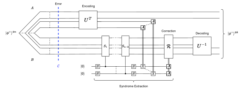
Following the construction proposed in Section II.2, we now present a purification protocol developed through an adaptation of QGRAND, which we will refer to as Purification GRAND (PGRAND). Let us assume an initial setup of Bell pairs shared between Alice and Bob through a noisy quantum channel . At the end of the protocol procedures, both parties will share Bell pairs with higher fidelity. The protocol is depicted in Figure 1 and can be summarized by the following steps:
-
1.
Apply a random encoding on Alice’s qubits. Share the encoding information with Bob.
-
2.
Perform single-qubit measurements in the computational basis on of Alice’s qubits, followed by the classical transmission of the measurement outcomes to Bob.
-
3.
With the information about the encoding, simulate the stabilizer circuit and determine the stabilizers for the qubits which were initially entangled with the measured ones. Measure the syndrome using all the determined stabilizers.
-
4.
Update the syndrome obtained with the information received.
-
5.
Use a noise guessing approach to identify the error pattern and apply the recovery procedure on the corrupted state.
-
6.
Apply the decoding at B. Discard the measured pairs and keep the remaining ones.
III.1.1 Encoding
The protocol starts by applying an encoding on Alice’s qubits, composed of randomly selected 2-qubit Clifford gates. To do so, one can generate a random tensor product of Clifford gates, transpose it, and apply it to the initial state. The information about the original tensor product has to be sent classically to Bob. Alternatively, both parties could previously agree on the random encoding to be used. To obtain a highly performant code, Clifford gates are required on average [34]. As most of the gates can be applied in parallel, the encoding has a circuit depth of .
III.1.2 Determining the stabilizers
After the qubits are generated and subjected to noise, the process of gathering information about the state is limited to local operations. To overcome that issue, we can still make use of local stabilizers on Bob’s qubits, but it is required that the respective entangled qubits on Alice’s side be measured. After some initial state has been encoded with an unitary transformation , the stabilizers of the encoded state can be obtained by evolving the initial stabilizers through the encoding, that is, if is a stabilizer of the initial state, then is a stabilizer of the final encoded state since
| (10) |
Although the proposed protocol performs the measurements after the encoding operation, given Equation 2 it is possible to assume that, for those qubits that are being measured, the measurements on Alice’s side are performed before the encoding operation on Bob’s side. Hence, we can focus our attention in evolving the stabilizers of the measured states. If the initial state is a Bell pair, the operators and are able to stabilize locally on Bob’s side the states obtained after a -measurement of a Bell pair, and , respectively. Hence, each stabilizer can be evolved through , that is, we obtain the stabilizers and . Since , changing the stabilizers according to the measurement is equivalent to performing a classical bit-XOR operation of the syndrome with the measurement result.
III.1.3 Noise guessing and correction
Bob can efficiently simulate the encoding circuit and build a parity check matrix to map each error pattern to the respective syndrome. With the noise statistics, Bob can determine the most likely error associated with a syndrome, so that whenever that syndrome is measured, the recovery procedure is done such that the most likely error is selected and corrected.
Since the possible number of error patterns increases exponentially on the number of qubits for most of the error models, Bob might only be able to precompute the syndromes associated with a fraction of the total possible errors. The number of syndromes that are computed should be chosen according to the initial fidelity of the pairs, the number of qubits and the required final fidelity. This approach will save resources and make the computation possible at the cost of a decrease in performance. The computation of the syndrome of each error pattern involves multiplying a -bit array representing the error with a matrix representing the stabilizers, requiring time. In practice, this procedure can be efficiently parallelized. When aiming to correct the error patterns with a weight up to , we may take advantage of previously computed syndromes for lower weight errors to achieve a computation cost in obtaining the syndrome table.
It is important to note that this step is the primary limiting factor in what regards the classical computational cost, just like in the case of the hashing protocol [26, 29], with the circuit simulation playing a negligible role in the overall cost.
After mapping each error pattern with a syndrome, only the most likely error pattern associated to each syndrome needs to be stored, and the remaining can be discarded. The number of possible error patterns is and is the number of available syndromes. Whenever a syndrome is extracted, all that is needed to identify the recovery procedure is a linear search on a table of at most size , which requires space and time to store the syndromes and perform a search.
III.1.4 Decoding
As outlined in the protocol’s presentation, the decoding entails reversing the encoding operation and discarding the measured qubits. Nevertheless, since only Clifford gates are used in the decoding, a virtual execution prior to the recovery operation is also feasible. In that case, all that needs to be done is to make the appropriate adjustments to the recovery operation. Both the decoding (except for the discarding of pairs) and the correction involve Clifford gates, so all of this can be performed classically through software [53].
Overall, for a single PGRAND application that uses Bell pairs to obtain , the overhead per pair, that is, the number of qubits that are spent in the use of the protocol, is given by (due to the qubits that are required to be measured and the qubits that are used as ancillas). For the syndrome extraction, each of the stabilizer applications is composed by, on average, CNOT gates and single-qubit gates, requiring a total of gates.
III.2 Results
Consider a setup of Werner states with initial fidelity , with being the parameter of a depolarizing channel. Define to be the map between each error pattern and its weight. Let be the number of possible error patterns with weight and the number of possible error patterns with equal or less weight than . For depolarizing noise these quantities are given by
| (11) |
Let be the binomial probability mass function. For each error pattern , we have that
| (12) |
from which we immediately conclude that for any (as long as ).
The approach of correcting the most likely errors in this noise scenario prioritizes the correction of lower-weight errors. That is, for a set of error patterns that share the same syndrome, the protocol considers the error that has occurred to be the error pattern with the lowest weight.
Under the assumption that any correctly identified error can be completely corrected, it is useful for the analysis of the protocol to define the correctable fraction of weight as
| (13) |
Then, if degenerate scenarios are disregarded, the average correctable fraction is approximately [34]
| (14) |
Note that computing the syndromes associated with every possible error pattern has a high computational cost and it might be impossible even for relatively small values of . Thus we introduce a threshold parameter that defines the maximum weight of the error patterns for which the syndromes are computed, implying that . Now we can compute probability of error of the protocol as follows
| (15) |
This provides a useful lower bound for the achieved average fidelity, , of the output pairs, as explained in Appendix A. Therefore, we say that the protocol achieves purification if one obtains that .
The efficiency of a protocol is determined by its yield, which is normally defined as the ratio between the number of purified pairs with fidelity arbitrarily close to unity and the initial number of pairs required by the protocol. Such a definition would imply that many protocols would have a zero yield, including the hashing protocol when employed for finite-sized ensembles. Therefore, we shall consider a relaxed version of this definition. Given some target fidelity , we consider the yield to be the ratio between the number of obtained states with fidelity greater than and the number of initial noisy copies.
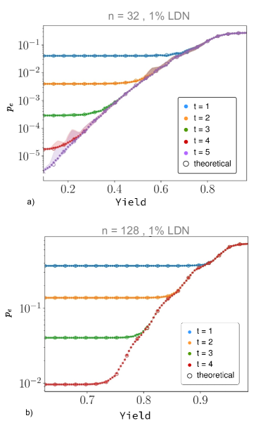
To assess the accuracy of the results obtained using Equation 14, the random encoding was simulated by generating a random parity check matrix, and the syndromes for each considered error pattern were computed using the techniques explained in Ref. [51]. This was performed considering 32 and 128 Bell pairs, affected by 1% LDN. The results are shown in Figure 2. These results were obtained for each value by performing twenty Monte Carlo simulations for each yield value considered. In the figure, each data point represents the average result of these simulations.
Given the computational complexity and hardware constraints associated with conducting these extensive simulations, the subsequent findings in this section are derived from their analytical approximations. The numerical results obtained using these expressions for various values of , , and can be found in Appendix C
The approach of correcting the most likely errors implies that, in order to achieve purification, at least all the error patterns with weight up to must be considered by the protocol.
The capacity (i.e., the highest rate or yield one can possibly obtain using a quantum error correction code and PP) of the depolarizing channel for non-degenerate stabilizer codes is upper bounded by
| (16) |
where is the binary entropy function [54]. This bound is known as the quantum Hamming bound, and it can be exceeded by degenerate codes [55]. Although the capacity of the depolarizing channel has already been determined [56, 57], this bound provides a more manageable expression for evaluating the performance of a stabilizer code in a setup that involves a large number of channel uses.
Using similar arguments as the ones in [58], one can prove that the yield of our protocol is upper bounded by this bound. However, it is worth evaluating how close the yield requirements are to that bound. Assuming an initial fidelity , Figure 3 illustrates the maximum yield required to achieve an error probability below a specified threshold. These results are derived without imposing any constraints on the weight of the errors considered. Thus, the number of available syndromes emerges as the sole limiting factor influencing the outcomes.
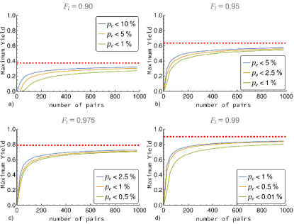
The most significant observation from fig. 3 is the initial growth in the required yield as the number of pairs increases up to a few hundred. Notably, by employing the protocol on ensembles with a few more qubits, much superior efficiencies can be obtained. However, using more than five hundred pairs leads to only marginal changes in the yield required to obtain the same error probabilities, since in this regime the yield is already close to the capacity of the channel. This observation may have critical implications for the realistic implementation of the protocol, as the challenge of generating and manipulating larger qubit ensembles could pose a substantial obstacle. Another noteworthy aspect is the minimal difference in the required yields for achieving pairs with varying error probabilities. This is evident by the proximity between the curves in each plot, indicating that a much more purified state can be obtained by slightly sacrificing the protocol’s yield.
III.3 Computational limitations
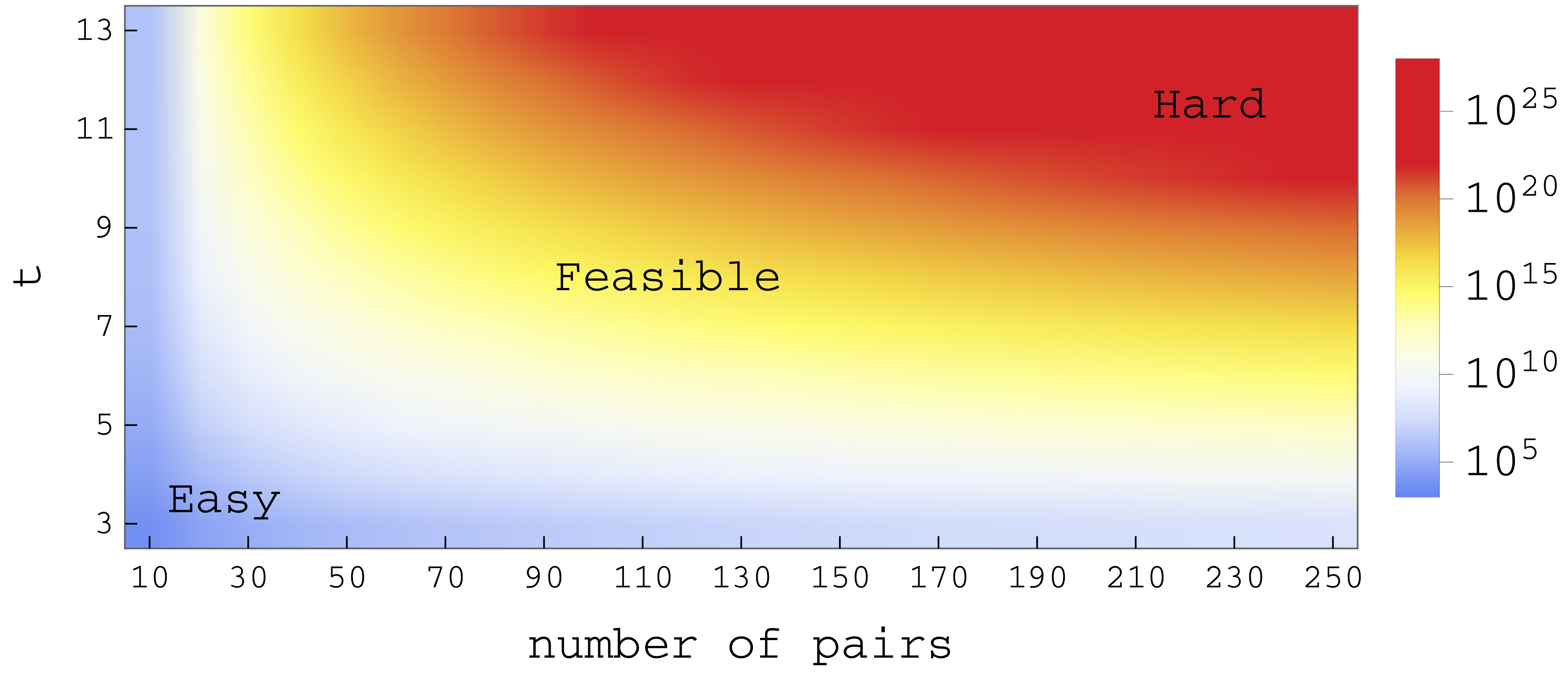
In some situations, it may prove infeasible to account for error patterns that are extremely unlikely, such as those with very high weight, when the noise model is a Pauli channel. Figure 4 showcases the regimes that are more realistic to consider.
As we limit the correction process to only account for error patterns with weight at most , PGRAND’s performance may be degraded. In Figure 5 it is possible to see the minimum value of fidelity needed to achieve purification, , according to the number of pairs and the constraint imposed on the value of . If no constraints were imposed, this value is expected to solely decrease with the number of pairs, since in this scenario the only limiting factor is the number of available syndromes.
However, following section III.1.3, if one limits the number of error patterns considered, a saturation point is reached. In this scenario, the number of possible syndromes surpasses the number of considered error patterns, and no advantage is obtained by having more syndromes. As the number of pairs increases, errors with greater weight become more likely, causing an increase in the error probability and the value of .
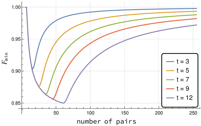
| 6 | 7 | 8 | 9 | 10 | 11 | 12 | |
| 30 | 35 | 40 | 45 | 50 | 56 | 61 | |
| 0.8695 | 0.8642 | 0.8601 | 0.8578 | 0.8542 | 0.8512 | 0.8499 |
It is also possible to determine a bound for the value of regardless of the number of pairs, following a similar reasoning as the one used in Ref. [26]. Indeed, given that the yield of the protocol is bounded by Equation 16, a positive yield can only be obtained as long as , that is, .
IV Comparison of approaches
A similar approach to purification is performed by the Hashing protocol. The Hashing protocol [26] is a one-way entanglement purification protocol that operates on a large ensemble of noisy entangled pairs. Representing by the density matrix of the initial ensemble, the hashing protocol is capable of distilling a smaller number of pairs , where is the Von Neumann entropy, with fidelity arbitrarily close to unity in the asymptotic regime where .
The protocol consists of rounds where, at each round one of the parties performs some unitary operations and one of the qubits is measured and sacrificed to reveal information about the system, with each measurement revealing one bit about the unmeasured pairs. The result of the measurement is sent classically to the other party, which by measuring the corresponding qubit obtains information about the parity of the ensemble.
For a small parameter , the protocol attempts to correct errors that belong to the following set
| (17) |
While the original intention of the hashing protocol was to operate with an asymptotically large number of Bell pairs, our interest is to assess its performance with a finite (and possibly small) ensemble. For this reason, we consider the yield of the hashing protocol with rounds to be given by .
Nonetheless, we present a comparison of performance between PGRAND and this protocol. The first challenge of establishing a fair comparison lies in the absence of a straightforward expression for the fidelity of the states produced by the hashing protocol. To enable the comparison, we rely on a bound derived in Ref. [59] concerning the average fidelity achieved by the hashing protocol when applied to Werner states with fidelity parameter . The bounding expression is as follows:
| where | |||
This bound was established by bounding the probability of failure of the hashing protocol
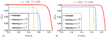
The parameter presents a challenge to our comparison, as its smaller values prompt the hashing protocol to attempt to correct a larger number of error patterns, as stipulated by eq. 17. However, if the yield is not sufficiently small, an increase in leads to a reduction in the fidelity of the output pairs ( see Appendix B). This trade-off is evident in Figure 6, where we compare the fidelity achieved by PGRAND (without imposing a restriction on the number of corrected errors) to that achieved by the hashing protocol, for similar values of as the ones used in other references [26, 59, 31].
Nevertheless, it is clear that PGRAND outperforms the hashing protocol, particularly when 128 pairs are used. For the hashing protocol fails to achieve purification for the number of pairs considered.
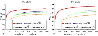
Next, we compare how the initial pair count in the ensemble changes the yield required for purification (). The results in Figure 7 show us that the hashing protocol demands a larger ensemble of pairs. The increase of the number of pairs enables the use of a greater value for the parameter , leading to higher yields. It becomes clear that as increases the hashing protocol performance approaches the performance of our protocol. In the considered noise scenarios, using higher values of would lead to similar yields for both protocols.
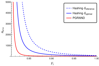
To evaluate the minimum number of pairs required, denoted as , for achieving purification, the protocols were examined under the condition where only one purified pair is generated. Specifically, this corresponds to the case where , enabling the establishment of a limiting scenario. For the PGRAND evaluation, no constraints were imposed on the value of (which corresponds to considering ).
When setting for the hashing protocol, it is common in the literature to use [59, 31]. However, this choice of is suboptimal, as demonstrated in Figure 8, where we compare the values of for our protocol and the hashing protocol. Therefore, we include a comparison with the results obtained by the hashing protocol when selecting an that maximizes the fidelity for each considered fidelity value . The results at some notable points of the curves are detailed in Table 2.
| 0.83 | 0.85 | 0.90 | 0.95 | 0.99 | |
|---|---|---|---|---|---|
| PGRAND | 251 | 60 | 16 | 10 | 8 |
| Hashing | 2326 | 637 | 153 | 71 | 45 |
| Hashing | 8116 | 2027 | 412 | 164 | 82 |
There is a clear exponential relationship between and , and as expected, the higher the initial fidelity the fewer initial pairs are required to achieve purification. For example, while for achieving purification with it is required that , for we have that . Nevertheless, employing as few as 10 qubits enables the purification of states with , while increasing the qubit count to 16 lowers this threshold to . This is in striking contrast with the hashing protocol, which requires at least an ensemble with a size in the order of the hundred qubits for most noise regimes.
For a practical scenario, it is crucial to assess the performance of both protocols under equivalent computational constraints. This entails examining how they fare when correcting a comparable number of errors. However, while PGRAND’s performance improves with the number of errors it aims to correct (set by the parameter ), the hashing protocol doesn’t necessarily follow the same trend. Increasing the number of errors under consideration (represented by a lower value of ) may result in a decline of its performance, as detailed in Appendix B, making direct comparisons challenging.
Nonetheless, we define and compare the fidelity achieved by the hashing protocol using with the fidelity attained by PGRAND when limiting the error correction to errors with weight up to . The choice of a suitable value for is made to ensure a fair and balanced comparison with PGRAND under similar error correction conditions. For both protocols, we considered the scenario where only one purified pair is obtained (). Therefore the results depicted in Figure 9 serve only to illustrate how both protocols perform under the same computational constraints.
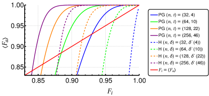
We observe that for a small number of pairs, PGRAND exhibits superior performance compared to the hashing protocol. As the number of pairs in the initial ensemble increases, the performance differences between the two approaches tend to diminish. However, it is crucial to consider the computational cost associated with larger initial ensembles. The hashing protocol becomes impractical due to this increased computational burden, while PGRAND maintains the advantage of achieving purification with a smaller number of pairs and manageable computational resources.
PGRAND appears to offer a distinct improvement over the hashing protocol. However, its implementation demands more gates and qubits compared to the hashing protocol; while both require gates, the hashing protocol does not use ancilla qubits. Consequently, the advantage of using PGRAND might be diminished if one considers the noise introduced by each gate.
V Measurement-based version of PGRAND
During the analysis of the protocol we assumed that the operations were noiseless. Nonetheless, this is an unrealistic approach, and even a slight amount of noise can compromise the entire protocol, since the entropy of the ensemble is amplified by each noisy operation. Considering that two-qubit operations are required, the increase in entropy caused by noisy operations can easily exceed the information obtained from the measurement. This holds even for minor imperfections, posing a threat to the entire protocol.
Although Clifford gates can be implemented in a fault tolerant manner, this problem can be circumvented by using a measurement-based approach. The main concept revolves around the preparation of a resource state using measurement-based methods, which incorporate both the encoding, stabilizer measurement, and decoding of the protocol. Afterward, the Bell pairs are coupled to the resource state using Bell measurements 111Executing the purification protocol in this manner renders it non-deterministic due inherent probabilistic nature of Bell measurements., in a manner similar to what is carried out in Refs. [61, 62, 36, 37, 31, 63].
For an entanglement purification protocol that uses only Clifford gates to distill pairs from an initial ensemble of pairs, a minimal resource state can be obtained with qubits. Although the measurement-based approach requires more qubits, ancilla qubits are not needed, as explained in [38, 46]. Additionally, any Clifford circuit can be implemented using only one measurement layer, that is, with all measurements being parallelizable. However, it is essential to note that, despite the resulting state is no longer a cluster state (and therefore is no longer universal) it is, up to local unitaries, equivalent to a graph state [38, 64].
The resource states can be obtained from a cluster state and then purified and encoded. Quantum communication via measurement-based entanglement purification has been shown to outperform direct transmission, gate-based error correction, and measurement-based schemes generating resource states directly [65].
The fact that the resource state can be prepared in advance is especially relevant because qubits may experience dephasing during the processing time of the protocol. However, with the resource state prepared beforehand, the processing time is uniquely limited to the time required to perform the Bell measurements and classically communicate the results.
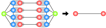
To estimate the error thresholds in a noisy scenario for this protocol, we remark that it has been proven that it is possible to formally transfer the noise affecting the input qubits of the resource state to the Bell pairs targeted for purification [62]. Consider that the Bell pairs and the resource states are affected by LDN with parameters and respectively.
It is easily verifiable through simple computations that this is equivalent to considering that one starts with Werner states with fidelity
| (19) |
Similarly, the noise present in the output qubits can also be transferred to the final state, given that one can always assume that the protocol outputs Werner states with fidelity . Thus, after moving the noise from the output qubits of the resource state to the output Bell pairs, one ends up again with a Werner state with fidelity
| (20) |
The advantage of this decomposition is that, once the noise has been transferred, we are left with a perfect purification process to which our previously presented analytical results still apply. With that in mind, we can now deduce a threshold for the tolerable error value of the resource states. By recognizing that it is impossible to purify Bell pairs with a fidelity lower than that of the resource state, we obtain the condition . This condition arises from the requirement that the purification process must be achievable, which imposes . Moreover, the protocol can only operate on a depolarized state with fidelity . Hence the following condition is obtained
| (21) |
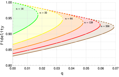
implying the threshold to be . Figure 11 presents a numerical analysis of the purification ranges corresponding to various numbers of initial pairs, while Table 3 displays the error thresholds for the same numbers of initial pairs. These thresholds for the minimum required fidelity and the maximum achievable fidelity were obtained by inspecting the -to-one routine. These values can be seen in Table 4 and Table 5, respectively.
| Error Threshold | |||||
|---|---|---|---|---|---|
| 16 | 32 | 64 | 128 | 256 | |
| 1.72% | 3.39% | 4.79% | 5.96% | 6.89% | |
VI Conclusion
Quantum entanglement purification methods are vital in quantum information processing. They help mitigate noise and enable the recovery of highly entangled states, making them essential tools for various quantum information tasks.
In this paper, we present a purification protocol that represents a significant improvement over Bennett’s hashing protocol. We provide a detailed explanation of the protocol’s construction concepts and the underlying principles, along with a comprehensive analysis of its performance across different ensemble sizes, noise regimes, and computational constraints.
Our findings demonstrate that our protocol can achieve a fidelity of 90% when purifying states, even with a relatively small ensemble size of just 16 Bell pairs. While hashing protocols offer distinct advantages over other types of protocols due to their non-probabilistic nature (unlike recurrence protocols) and high performance as the initial ensemble size increases, they are constrained by the computational resources they require [29, 59, 36]. The requirement of such a small initial ensemble in our protocol not only reduces computational costs significantly but also paves the way for a more realistic implementation. This is especially relevant in practical scenarios where there is a preference for employing fewer qubits. Moreover, if one manages to obtain a larger ensemble of Bell pairs with sufficiently low levels of noise, high efficiencies can be obtained while maintaining a feasible computational cost. Thus, PGRAND purports to be specially relevant in low-entropy noise regimes.
The assumption of using noiseless gates can be overcome by using a measurement-based implementation of these protocols. Moreover, the general fault-tolerance of a gate implementation of QGRAND is subject of ongoing work.
The extension of our protocol to multipartite entanglement is also an interesting question to study. Given that the Bell matrix identity can generalized to GHZ states [66], a version of the protocol to these states should be conceivable. Furthermore, the performance of our protocol could be improved by considering its generalization to multi-level systems (qudits), since notable improvements were found for a bipartite qudit implementation of the hashing protocol [31]. It would also be worthy to study in a more detailed scenario the feasibility of the measurement-based of this protocol, and how the cluster state size/complexity would influence the error of the resource states in a realistic implementation.
Acknowledgments
Francisco Monteiro and Bruno Coutinho are grateful to Prof. Wolfgang Dür (University of Innsbruck) for insightful discussions about hashing-based purification. We thank FCT/MCTES (Portugal) for its support through national funds and when applicable co-funded EU funds under projects UIDB/50008/2020 and 2022.05558.PTDC. Diogo Cruz acknowledges the support from FCT through scholarship UI/BD/152301/2021.
References
- Kimble [2008] H. J. Kimble, The quantum internet, Nature 453, 1023 (2008).
- Caleffi et al. [2018] M. Caleffi, A. S. Cacciapuoti, and G. Bianchi, Quantum internet: from communication to distributed computing!, in Proceedings of the 5th ACM International Conference on Nanoscale Computing and Communication (ACM, Reykjavik Iceland, 2018) pp. 1–4.
- Wu et al. [2020] A.-K. Wu, L. Tian, B. C. Coutinho, Y. Omar, and Y.-Y. Liu, Structural vulnerability of quantum networks, Phys. Rev. A 101, 052315 (2020).
- Horodecki et al. [2009] R. Horodecki, P. Horodecki, M. Horodecki, and K. Horodecki, Quantum entanglement, Reviews of Modern Physics 81, 865 (2009).
- Bennett and Brassard [2014] C. H. Bennett and G. Brassard, Quantum cryptography: Public key distribution and coin tossing, Theoretical Computer Science 560, 7 (2014).
- Bennett et al. [1993] C. H. Bennett, G. Brassard, C. Crépeau, R. Jozsa, A. Peres, and W. K. Wootters, Teleporting an unknown quantum state via dual classical and einstein-podolsky-rosen channels, Physical Review Letters 70, 1895 (1993).
- Cirac et al. [1999] J. I. Cirac, A. K. Ekert, S. F. Huelga, and C. Macchiavello, Distributed quantum computation over noisy channels, Physical Review A 59, 4249 (1999).
- Dür and Briegel [2003] W. Dür and H.-J. Briegel, Entanglement Purification for Quantum Computation, Physical Review Letters 90, 067901 (2003).
- Sekatski et al. [2017] P. Sekatski, M. Skotiniotis, and W. Dür, Improved sensing with a single qubit, Physical Review Letters 118, 170801 (2017).
- Krutyanskiy et al. [2023] V. Krutyanskiy, M. Galli, V. Krcmarsky, S. Baier, D. A. Fioretto, Y. Pu, A. Mazloom, P. Sekatski, M. Canteri, M. Teller, J. Schupp, J. Bate, M. Meraner, N. Sangouard, B. P. Lanyon, and T. E. Northup, Entanglement of Trapped-Ion Qubits Separated by 230 Meters, Physical Review Letters 130, 050803 (2023).
- Figgatt et al. [2019] C. Figgatt, A. Ostrander, N. M. Linke, K. A. Landsman, D. Zhu, D. Maslov, and C. Monroe, Parallel entangling operations on a universal ion-trap quantum computer, Nature 572, 368 (2019).
- Bruzewicz et al. [2019] C. D. Bruzewicz, J. Chiaverini, R. McConnell, and J. M. Sage, Trapped-ion quantum computing: Progress and challenges, Applied Physics Reviews 6, 021314 (2019).
- Riedel et al. [2017] D. Riedel, I. Söllner, B. J. Shields, S. Starosielec, P. Appel, E. Neu, P. Maletinsky, and R. J. Warburton, Deterministic enhancement of coherent photon generation from a nitrogen-vacancy center in ultrapure diamond, Physical Review X 7, 031040 (2017).
- Ruf et al. [2019] M. Ruf, M. IJspeert, S. Van Dam, N. De Jong, H. Van Den Berg, G. Evers, and R. Hanson, Optically coherent nitrogen-vacancy centers in micrometer-thin etched diamond membranes, Nano Letters 19, 3987 (2019).
- Kaufman et al. [2015] A. M. Kaufman, B. J. Lester, M. Foss-Feig, M. L. Wall, A. M. Rey, and C. A. Regal, Entangling two transportable neutral atoms via local spin exchange, Nature 527, 208 (2015).
- Madjarov et al. [2020] I. S. Madjarov, J. P. Covey, A. L. Shaw, J. Choi, A. Kale, A. Cooper, H. Pichler, V. Schkolnik, J. R. Williams, and M. Endres, High-fidelity entanglement and detection of alkaline-earth Rydberg atoms, Nature Physics 16, 857 (2020).
- Leung et al. [2019] N. Leung, Y. Lu, S. Chakram, R. K. Naik, N. Earnest, R. Ma, K. Jacobs, A. N. Cleland, and D. I. Schuster, Deterministic bidirectional communication and remote entanglement generation between superconducting qubits, npj Quantum Information 5, 1 (2019).
- Flurin et al. [2015] E. Flurin, N. Roch, J. D. Pillet, F. Mallet, and B. Huard, Superconducting Quantum Node for Entanglement and Storage of Microwave Radiation, Physical Review Letters 114, 090503 (2015).
- Roffe [2019] J. Roffe, Quantum error correction: an introductory guide, Contemporary Physics 60, 226 (2019).
- Devitt et al. [2013] S. J. Devitt, W. J. Munro, and K. Nemoto, Quantum error correction for beginners, Reports on Progress in Physics 76, 076001 (2013).
- Munro et al. [2015] W. J. Munro, K. Azuma, K. Tamaki, and K. Nemoto, Inside Quantum Repeaters, IEEE Journal of Selected Topics in Quantum Electronics 21, 78 (2015).
- Duan et al. [2001] L.-M. Duan, M. D. Lukin, J. I. Cirac, and P. Zoller, Long-distance quantum communication with atomic ensembles and linear optics, Nature 414, 413 (2001).
- Santos et al. [2023] S. Santos, F. A. Monteiro, B. C. Coutinho, and Y. Omar, Shortest Path Finding in Quantum Networks With Quasi-Linear Complexity, IEEE Access 11, 7180 (2023).
- Bugalho et al. [2023] L. Bugalho, B. C. Coutinho, F. A. Monteiro, and Y. Omar, Distributing Multipartite Entanglement over Noisy Quantum Networks, Quantum 7, 920 (2023).
- Coutinho et al. [2023] B. C. Coutinho, R. Monteiro, L. Bugalho, and F. A. Monteiro, Entanglement routing based on fidelity curves for quantum photonics channels (2023), arXiv:2303.12864 [quant-ph] .
- Bennett et al. [1996a] C. H. Bennett, D. P. DiVincenzo, J. A. Smolin, and W. K. Wootters, Mixed-state entanglement and quantum error correction, Physical Review A 54, 3824 (1996a).
- Bennett et al. [1996b] C. H. Bennett, G. Brassard, S. Popescu, B. Schumacher, J. A. Smolin, and W. K. Wootters, Purification of noisy entanglement and faithful teleportation via noisy channels, Physical Review Letters 76, 722 (1996b).
- Deutsch et al. [1996] D. Deutsch, A. Ekert, R. Jozsa, C. Macchiavello, S. Popescu, and A. Sanpera, Quantum Privacy Amplification and the Security of Quantum Cryptography over Noisy Channels, Physical Review Letters 77, 2818 (1996).
- Chau and Ho [2011] H. F. Chau and K. H. Ho, Practical entanglement distillation scheme using recurrence method and quantum low density parity check codes, Quantum Information Processing 10, 213 (2011).
- Krastanov et al. [2019] S. Krastanov, V. V. Albert, and L. Jiang, Optimized Entanglement Purification, Quantum 3, 123 (2019).
- Miguel-Ramiro and Dür [2018] J. Miguel-Ramiro and W. Dür, Efficient entanglement purification protocols for d-level systems, Physical Review A 98, 042309 (2018).
- Dür and Briegel [2007] W. Dür and H. J. Briegel, Entanglement purification and quantum error correction, Reports on Progress in Physics 70, 1381 (2007).
- Aschauer et al. [2005] H. Aschauer, W. Dür, and H.-J. Briegel, Multiparticle entanglement purification for two-colorable graph states, Physical Review A 71, 012319 (2005).
- Cruz et al. [2023] D. Cruz, F. A. Monteiro, and B. C. Coutinho, Quantum error correction via noise guessing decoding, IEEE Access 11, 10.1109/ACCESS.2023.3327214 (2023).
- Chandra et al. [2023] D. Chandra, Z. B. Kaykac Egilmez, Y. Xiong, S. X. Ng, R. G. Maunder, and L. Hanzo, Universal decoding of quantum stabilizer codes via classical guesswork, IEEE Access 11, 19059 (2023).
- Zwerger et al. [2014] M. Zwerger, H. J. Briegel, and W. Dür, Robustness of hashing protocols for entanglement purification, Physical Review A 90, 012314 (2014).
- Zwerger et al. [2016] M. Zwerger, H. J. Briegel, and W. Dür, Measurement-based quantum communication, Applied Physics B 122, 50 (2016).
- Raussendorf [2009] R. Raussendorf, Measurement-based quantum computation with cluster states, International Journal of Quantum Information 07, 1053 (2009).
- Raussendorf and Briegel [2001] R. Raussendorf and H. J. Briegel, A one-way quantum computer, Physical Review Letters 86, 5188 (2001).
- Duffy et al. [2019] K. R. Duffy, J. Li, and M. Médard, Capacity-Achieving Guessing Random Additive Noise Decoding, IEEE Transactions on Information Theory 65, 4023 (2019).
- Aschauer [2005] H. Aschauer, Quantum communication in noisy environments, Text.PhDThesis, Ludwig-Maximilians-Universität München (2005).
- Matsumoto [2003] R. Matsumoto, Conversion of a general quantum stabilizer code to an entanglement distillation protocol, Journal of Physics A: Mathematical and General 36, 8113 (2003), arxiv:quant-ph/0209091 .
- Werner [1989] R. F. Werner, Quantum states with einstein-podolsky-rosen correlations admitting a hidden-variable model, Physical Review A 40, 4277 (1989).
- Dür et al. [2005] W. Dür, M. Hein, J. I. Cirac, and H.-J. Briegel, Standard forms of noisy quantum operations via depolarization, Physical Review A 72, 052326 (2005).
- Raussendorf and Briegel [2002] R. Raussendorf and H. Briegel, Computational model underlying the one-way quantum computer (2002), arxiv:quant-ph/0108067 .
- Nielsen and Dawson [2005] M. A. Nielsen and C. M. Dawson, Fault-tolerant quantum computation with cluster states, Physical Review A 71, 042323 (2005).
- Dawson et al. [2006] C. M. Dawson, H. L. Haselgrove, and M. A. Nielsen, Noise Thresholds for Optical Quantum Computers, Physical Review Letters 96, 020501 (2006).
- Brown and Roberts [2020] B. J. Brown and S. Roberts, Universal fault-tolerant measurement-based quantum computation, Physical Review Research 2, 033305 (2020).
- Gimeno-Segovia et al. [2019] M. Gimeno-Segovia, T. Rudolph, and S. E. Economou, Deterministic generation of large-scale entangled photonic cluster state from interacting solid state emitters, Physical Review Letters 123, 070501 (2019).
- Dür et al. [2003] W. Dür, H. Aschauer, and H.-J. Briegel, Multiparticle Entanglement Purification for Graph States, Physical Review Letters 91, 107903 (2003).
- Gottesman [1998] D. Gottesman, The Heisenberg representation of quantum computers (1998), arxiv:quant-ph/9807006 .
- Aaronson and Gottesman [2004] S. Aaronson and D. Gottesman, Improved simulation of stabilizer circuits, Physical Review A 70, 052328 (2004).
- Paler et al. [2014] A. Paler, S. Devitt, K. Nemoto, and I. Polian, Software-based Pauli tracking in fault-tolerant quantum circuits, in 2014 Design, Automation & Test in Europe Conference & Exhibition (DATE) (2014) pp. 1–4.
- Ekert and Macchiavello [1996] A. Ekert and C. Macchiavello, Quantum error correction for communication, Physical Review Letters 77, 2585 (1996).
- DiVincenzo et al. [1998] D. P. DiVincenzo, P. W. Shor, and J. A. Smolin, Quantum-channel capacity of very noisy channels, Physical Review A 57, 830 (1998).
- Holevo [1998] A. Holevo, The capacity of the quantum channel with general signal states, IEEE Transactions on Information Theory 44, 269 (1998).
- King [2003] C. King, The capacity of the quantum depolarizing channel, IEEE Transactions on Information Theory 49, 221 (2003).
- Gottesman [1997] D. Gottesman, Stabilizer codes and quantum error correction (California Institute of Technology, 1997).
- Zwerger et al. [2018] M. Zwerger, A. Pirker, V. Dunjko, H. J. Briegel, and W. Dür, Long-range big quantum-data transmission, Physical Review Letters 120, 030503 (2018).
- Bennett [1962] G. Bennett, Probability inequalities for the sum of independent random variables, Journal of the American Statistical Association 57, 33 (1962).
- Zwerger et al. [2012] M. Zwerger, W. Dür, and H. J. Briegel, Measurement-based quantum repeaters, Physical Review A 85, 062326 (2012).
- Zwerger et al. [2013] M. Zwerger, H. J. Briegel, and W. Dür, Universal and Optimal Error Thresholds for Measurement-Based Entanglement Purification, Physical Review Letters 110, 260503 (2013).
- Yan et al. [2021] P.-S. Yan, L. Zhou, W. Zhong, and Y.-B. Sheng, Feasible measurement-based entanglement purification in linear optics, Optics Express 29, 9363 (2021).
- Hein et al. [2004] M. Hein, J. Eisert, and H. J. Briegel, Multiparty entanglement in graph states, Physical Review A 69, 062311 (2004).
- Wallnöfer and Dür [2017] J. Wallnöfer and W. Dür, Measurement-based quantum communication with resource states generated by entanglement purification, Physical Review A 95, 012303 (2017).
- Rengaswamy et al. [2022] N. Rengaswamy, A. Raina, N. Raveendran, and B. Vasić, Distilling GHZ states using stabilizer codes (2022), arxiv:2109.06248 [quant-ph] .
Appendix A Probability of error as a lower bound of the fidelity
We consider the probability of error to be the ratio between the number of successful uses of that protocol and the total number of uses. This can be interpreted as if any uncorrected error pattern maps the initial state to an orthogonal state, that is, , for any uncorrected error . If is a set of possible error patterns, and is the subset of correctable errors, then the average achieved fidelity of the state obtained at the end of the protocol verifies:
| (22) | ||||
| (23) | ||||
| (24) |
since it is considered that we are able to correct perfectly every error in , that is, . This is equivalent to model the output states of the protocol as Werner states with fidelity .
Appendix B Suboptimality of the hashing protocol
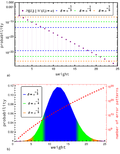
Consider the typical set as defined in Equation 17. Assuming that corresponds to the density matrix of a Werner state with parameter , the typical set encompasses all error patterns for which their probabilities satisfy
| (25) |
This set contains at most error patterns whose weight is closer to . As defined, the hashing protocol treats all errors within this set as equally important, implying that any error pattern in this set has the same probability of being corrected. However, this correction procedure is suboptimal, regardless of the choice of .
On one hand, a high value for will inherently limit the protocol’s performance, since even if it manages to correct all errors within the typical set, the total probability of error is upper-bounded by the sum of probabilities of errors that are not contained within the set. On the other hand, choosing a small value for implies the inclusion of many errors with relatively high weight. As the number of error patterns exponentially increases with their weight, it becomes more likely (for a fixed number of syndromes) that the corrected errors will be the ones with greater weight. However, each of these errors contributes only a small amount to the overall error probability of the protocol. In Figure 12, a practical scenario illustrates how the choice of interferes with the hashing protocol’s performance. For illustration purposes, we have selected an ensemble containing 128 qubits with 10% LDN, but the same holds true for other choices. Even with an optimal choice of and a sufficiently large , the correction procedure is never optimal. If we consider the computational cost of mapping each syndrome to an error pattern, it becomes evident how the hashing protocol will often fail to achieve purification for most practical cases.
Appendix C Additional numerical results
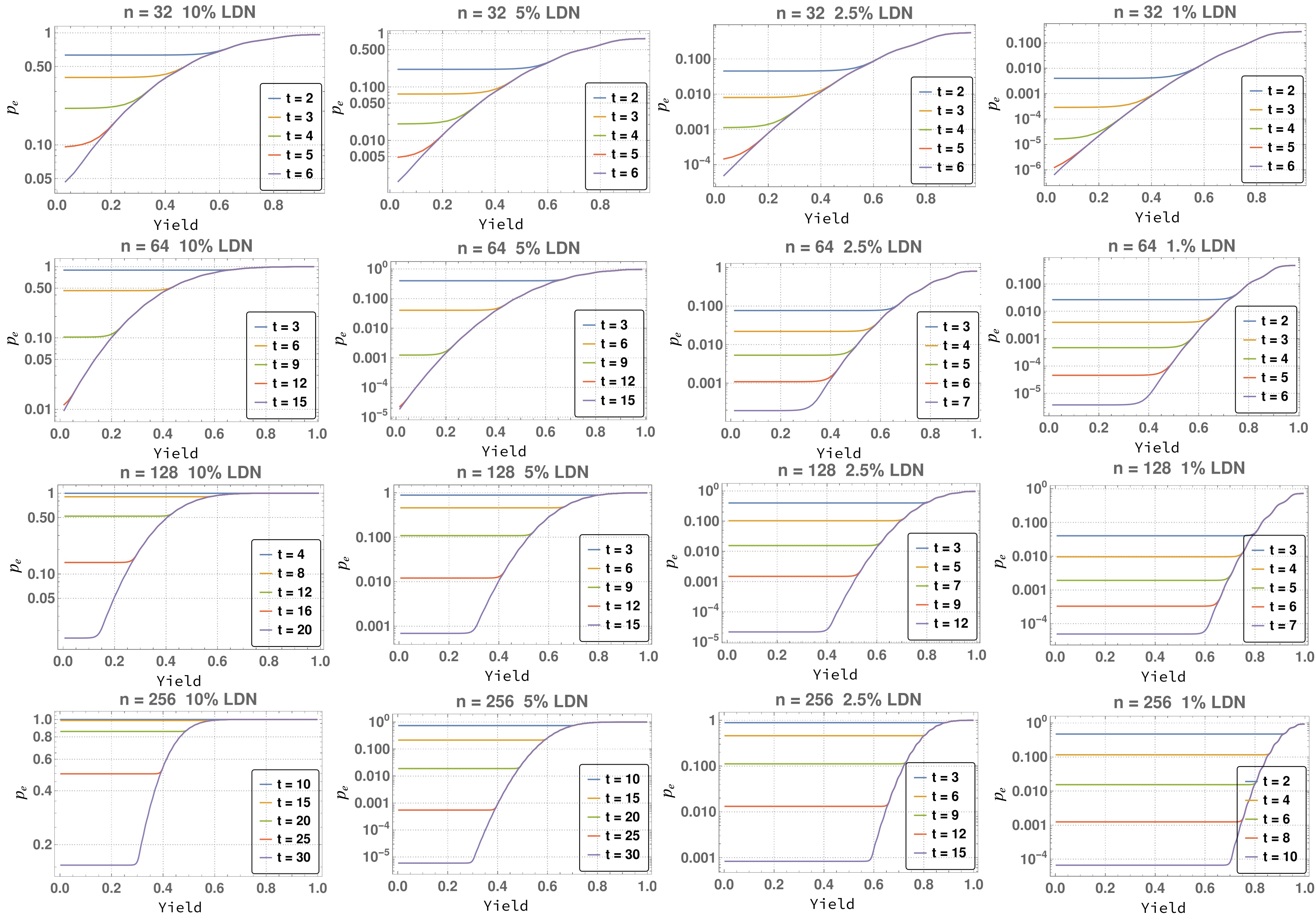
In this section, we present complementary numerical results. In Figure 13 is possible to see different results regarding the probability of error of the protocol, for different levels of noise, ensemble sizes and computational constraints. These values were obtained solely using the theoretical expressions Equation 14 and Equation 15. In Table 4 and Table 5 is possible to see the minimum fidelity required for purification, and the maximum achievable fidelity, respectively, for different degrees of error in the resource states and the sizes of the initial assemblies for the measurement-based version of the protocol.
| routine | 1% | 2% | 3% | 4% | 5% | 6% |
|---|---|---|---|---|---|---|
| -to- | .9238 | n/a | n/a | n/a | n/a | n/a |
| -to- | .8818 | .8996 | .9236 | n/a | n/a | n/a |
| -to- | .8608 | .8749 | .8890 | .9072 | n/a | n/a |
| -to- | .8479 | .8549 | .8711 | .8845 | .9002 | n/a |
| -to- | .8394 | .8494 | .8601 | .8713 | .8838 | .8984 |
| routine | 1% | 2% | 3% | 4% | 5% | 6% |
|---|---|---|---|---|---|---|
| -to- | .9878 | n/a | n/a | n/a | n/a | n/a |
| -to- | .9899 | .9795 | .9650 | n/a | n/a | n/a |
| -to- | .9899 | .9799 | .9699 | .9587 | n/a | n/a |
| -to- | .9899 | .9799 | .9699 | .9599 | .9496 | n/a |
| -to- | .9899 | .9799 | .9699 | .9599 | .9599 | .9398 |