Updated Proper Motion of the Neutron Star in the Supernova Remnant Cassiopeia A

Abstract

In this paper, we present updated estimates of the velocity of the neutron star (NS) in the supernova remnant (SNR) Cassiopeia A using over two decades of Chandra observations. We use two methods: 1.) recording NS positions from dozens of Chandra observations, including the astrometric uncertainty estimates on the data points but not correcting the astrometry of the observations, and 2.) correcting the astrometry of the 13 Chandra observations that have a sufficient number of point sources with identified Gaia counterparts. For method #1, we find velocity of 280 $\pm$ 123 km s^-1, with an angle of 87 $\pm$ 22 degrees south of east. For method # 2, we find a velocity of 445 $\pm$ 90 km s^-1 at an angle of 68 $\pm$ 12 degrees south of east. Both of these results match with the explosion-center-estimated velocity of $\sim$350 km s^-1 and the previous 10–year baseline proper motion measurement of 570 $\pm$ 260 km s^-1, but our use of additional data over a longer baseline has led to a smaller uncertainty by a factor of 2–3. Our estimates rule out velocities $\gtrsim$600 km s^-1 and better match with simulations of Cassiopeia A that include NS kick mechanisms.

1 Introduction

Neutron stars, the compact objects formed in some core-collapse supernovae (CCSNe), have typical observed velocities of hundreds of km s^-1 (Hobbs et al., 2005; Verbunt & Cator, 2017; Igoshev, 2020), with some sources reportedly reaching velocities of $\gtrsim$1000 km s^-1 (e.g., Chatterjee et al. 2005. These velocities are higher than can be explained from the disruption of a pre-explosion binary (v${}_{\rm NS}\approx 100$ km s^-1; Lai 2001), indicating that supernova explosion processes are responsible for these kicks. These velocities can be compared to various supernova remnant (SNR) properties—in particular, ejecta asymmetries—to provide constraints on supernova progenitors and explosion processes.

The two prevailing theories for the origins of NS kicks invoke conservation-of-momentum like arguments with asymmetric supernova explosion forces. In the first theory, hydrodynamical instabilities during a supernova lead to the NS being kicked in the opposite direction as the bulk of ejecta (Scheck et al., 2006; Wongwathanarat et al., 2013; Janka, 2017). In the second theory, both ejecta and NS move in a direction opposite the bulk of anisotropic neutrino emission (Fryer & Kusenko, 2006).

Recent observations and theoretical predictions have provided more support for the first scenario. 3D simulations have generated kick velocities of up to $\sim$700 km s^-1 in a direction opposite the bulk of ejecta (the “Gravitational Tugboat Mechanism’, see e.g., Wongwathanarat et al. 2013; Janka 2017; Gessner & Janka 2018). Observational studies have also confirmed that NSs are indeed preferentially kicked in a direction opposite the bulk ejecta motion in a sample of supernova remnants (SNRs) (Holland-Ashford et al. 2017; Katsuda et al. 2018; Bhalerao et al. 2019). As for the anisotropic neutrino emission scenario, although it is partially supported by an observed spin-kick alignment in some NSs (Johnston et al., 2005), generating kick velocities of $\sim$300 km s^-1 requires very strong ($\gtrsim$10¹⁶ G) magnetic fields (Scheck et al., 2006; Wongwathanarat et al., 2013)—unlikely, but still possible.

In order to use NSs as probes of SN explosion properties, it is vital to study NSs still embedded in SNRs. Such NSs can be directly linked to specific supernova explosions and compared to the SNR properties such as ejecta asymmetries, energy, distance, and age. However, these NSs are by definition young ($\lesssim$20 kyr old) and don’t exhibit radio, infrared, or optical emission, and thus astronomers are forced to largely rely on X-ray telescopes to study them. A typical NS velocity of $\sim$400 km s^-1 at a distance of 3 kpc corresponds to sky motion of only $\sim$0.03” yr^-1. Only Chandra has sufficient spatial resolution to measure the proper motions of NSs, and doing so requires baselines of at least a decade for all but the closest objects. There are currently $\sim$20 velocity measurements of NSs embedded within SNRs, found using a mix of direct proper motion measurements (e.g., Auchettl et al. 2015; Temim et al. 2017; Shternin et al. 2019; Mayer & Becker 2021; Long et al. 2022) and measuring the distance between NS positions and estimated SNR explosion sites (e.g., Winkler et al. 2009; Banovetz et al. 2021).

The SNR Cassiopeia A is the youngest known CCSNR in the Milky Way, with an age of $\sim$350 years and a distance of 3.33 $\pm$ 0.1 kpc (Fesen et al., 2006; Alarie et al., 2014). Its proximity and strong ejecta emission has enabled detailed investigation of its ejecta and shock emission on small, sub-parsec scales. Optical observations have shown that Cas A is an O-rich SNR (e.g., Chevalier & Kirshner 1978), and light echoes from the explosion reveal that Cas A was produced by an asymmetric Type IIb SN with variations in ejecta velocities of $\approx$4000 km s^-1 (Rest et al., 2011). The NS CXOU J232327.9$+$584842 was detected in the first-light image of Cas A (Tananbaum, 1999) and is a Central Compact Object (CCO), an odd class of neutron stars that are characterized by thermal emission, nonvariability, and weak magnetic fields (see e.g., Becker 2009; Halpern & Gotthelf 2010).

There are already a few estimates of the velocity of the NS in Cas A. Thorstensen et al. (2001) back-evolved the motion of various ejecta filaments to a central location, which should correspond to the origin of explosion (i.e., neutron star birth site). When combined with the SNR’s age and current NS location, this gives an indirect estimate of the NS’s velocity: $\sim$340 $\pm$ 30 km s^-1 at an angle of 78^∘ $\pm$ 8^∘ south of east.

As for direct proper motion measurements, both DeLaney & Satterfield (2013) and Mayer & Becker (2021) used Chandra HRC data from 1999 to 2009 to measure the proper motion of the NS. The former study made use of one background source and 13 quasi-stationary flocculi to correct for astrometric offsets between observations, reporting a velocity of 390 $\pm$ 400 km s^-1. The latter authors combined same-epoch HRC observations for more signal, detecting and using two background sources to find a proper motion estimate in RA of 18$\pm$12 mas/yr and in DEC of -35$\pm$17 mas/yr, for a total motion of 35$\pm$16 mas/yr and a velocity of 570 $\pm$ 260 km s^-1. The motivation of this paper is to use the additional 14 years of Chandra observation since 2009 to obtain a more precise NS velocity measurement.

In this paper, we present updated measurements of the proper motion of the CCO in Cas A using 24 years of Chandra X-ray observations, calculated using multiple methods. First, we measure its velocity without using background point sources to correct for Chandra astrometry, simply making use of dozens of observations of Cas A from 1999 to 2023. We include both detection uncertainty and astrometric uncertainty on the position of the NS at each epoch, fitting a line of best-fit to measure the overall motion. Using this method, each individual data point has large ($\gtrsim$0.5”) uncertainties, but the each additional data point enables a more precise measurement. In our second method, we use detected background point sources in observations of Cas A to improve for Chandra’s astrometric accuracy. The precision of the NS’s position at each epoch can be resolved down to $\sim$0.1”, but there are only a few observations with a sufficient number of detected calibration point sources with which to perform astrometry.

Our paper is formatted as follows: in Section 2, we describe our data and the procedures used to reprocess and analyze it. In Section 3, we present both of our velocity estimates along with any caveats. In Section 4, we discuss and compare our estimates to past works, both relating to Cas A specifically and to identified SNR & NS populations.

Table 1: Chandra Observations

ObsID	Date	Roll	Exposure	Det	ObsID	Date	Roll	Exposure	Det
		Angle ($\deg$)	(ks)				Angle ($\deg$)	(ks)
ACIS Observations (36 total; 32 usable)					HRC Observations (29)
114	2000-01-30	323.38	50	ACIS-S	171	1999-09-03	170.52	9	HRC-I
1952	2002-02-06	323.38	50	ACIS-S	172	1999-09-05	172.69	9	HRC-S
4634	2004-04-28	59.22	148	ACIS-S	1038	2001-09-19	186.64	50	HRC-S
4635	2004-05-01	59.22	138	ACIS-S	1505	1999-12-19	287.13	49	HRC-I
4636	2004-04-20	49.77	150	ACIS-S	1549	2001-04-04	311.1	5	HRC-I
4637	2004-04-22	49.77	170	ACIS-S	1550	2001-07-13	127.5	5	HRC-I
4638	2004-04-14	40.33	170	ACIS-S	1857	2000-10-04	204.45	48	HRC-S
4639	2004-04-25	49.77	80	ACIS-S	2781	2002-02-06	329.3	5	HRC-I
5196	2004-02-08	325.5	50	ACIS-S	3705	2003-10-19	220.7	5	HRC-I
5319	2004-04-18	49.77	40	ACIS-S	5157	2004-10-29	233.5	5	HRC-I
5320	2004-05-05	65.14	54	ACIS-S	5164	2004-03-15	5.8	4	HRC-I
6690	2006-10-19	221.14	62	ACIS-S	6038	2005-10-23	225.9	5	HRC-I
9117	2007-12-05	278.13	25	ACIS-S	6069	2005-04-12	36.9	5	HRC-I
9773	2007-12-08	278.13	25	ACIS-S	6739	2006-03-22	12.8	5	HRC-I
10935	2009-11-02	239.68	23	ACIS-S	6746	2006-10-15	215.9	5	HRC-I
10936	2010-10-31	236.48	31	ACIS-S	8370	2007-03-10	359.0	5	HRC-I
12020	2009-11-03	239.68	22	ACIS-S	9700	2008-03-24	15.2	5	HRC-I
13177	2010-11-02	236.48	17	ACIS-S	10227	2009-03-20	11.00	131	HRC-S
13783	2012-05-05	65.04	63	ACIS-S	10228	2009-03-28	24.86	130	HRC-S
14229	2012-05-15	75.44	50	ACIS-S	10229	2009-03-24	13.66	48	HRC-S
14480	2013-05-20	75.14	50	ACIS-S	10698	2009-03-31	23.20	51	HRC-S
14481	2014-05-12	75.14	50	ACIS-S	10892	2009-03-26	13.66	124	HRC-S
14482	2015-04-30	67.13	50	ACIS-S	11240	2009-12-20	287.02	12	HRC-I
16946	2015-04-27	54.97	68	ACIS-S	11955	2010-04-12	39.89	9	HRC-I
17639	2015-05-01	67.13	43	ACIS-S	12057	2009-12-13	287.02	10	HRC-I
18344	2016-10-21	214.20	26	ACIS-S	12058	2009-12-16	287.01	9	HRC-I
19604	2017-05-16	76.58	50	ACIS-S	12059	2009-12-15	287.02	12	HRC-I
19605	2018-05-15	75.23	49	ACIS-S	24840	2020-10-18	220.84	14	HRC-I
19606	2019-05-13	75.14	49	ACIS-S	26440	2022-07-05	121.49	4	HRC-I
19903	2016-10-20	214.20	25	ACISS
22426	2020-05-11	72.65	48	ACIS-S
23248	2020-05-14	72.65	28	ACIS-S
26248	2022-01-25	309.13	25	ACIS-I
26655	2022-12-30	297.17	29	ACIS-S
27099	2023-01-02	300.00	37	ACIS-S
27100	2023-01-15	310.11	27	ACIS-S

2 Observations and Data Analysis

2.1 Chandra Observations

Cas A was the target of Chandra’s first light image in 1999 (Hughes et al., 2000), and since then, Chandra has observed the SNR hundreds of times for over 3 Ms. However, most are calibration observations with observation times of a few kiloseconds: too short to measure a robust NS position, let alone fainter background sources for astrometric correction. We collected all ACIS and HRC imaging observations with observation times longer than a few kiloseconds, using the CIAO version 4.13 tool chandra_repro to reprocess the observations. Our list of observations—36 ACIS and 29 HRC—is reported in Table 1.

We removed observations with high chip offsets from our sample. Such offsets from the detector focal plane introduce additional astrometric uncertainties/offsets that would interfere with our ability to measure NS positions at each epoch. In total, we removed 4 observations with high ($\sim$10.7 mm) SIM-Z offsets—ACIS ObsIDs 6690, 13783, 16946, and 26248.

2.2 Point Source Detection

We ran the CIAO tool wavdetect on each of the observations in order to identify potential calibration point sources and then cross-matched detected point sources with known sources from the Gaia DR3 catalog (Gaia Collaboration et al., 2016, 2023; Babusiaux et al., 2023). If there was spatial coincidence, we verified the that: 1.) they remained coincident with Gaia counterparts across multiple epochs of observations, 2.) their spectra were distinct from ejecta emission, and 3.) they could be easily disentangled from surrounding SNR emission.

Across all observations, we detected 5 different point sources to use for astrometric correction. Figure 1 shows an image of Cas A with the point sources’ locations indicated, and Table 2 lists their properties and the observations they are detected in. Although we detected 5 reference point sources to use for calibration, no single point source was present in all observations. We ended up using 13 observations—5 HRC and 8 ACIS— that had a sufficient number of calibration point sources: $\geq$2 in most cases, but we loosen our restrictions to 1 for the latest observations taken in the past 5 years.

Table 2: Detected Point Sources

	1	2	3	4	5
Gaia DR3 Source ID 20104…	78284367990016	77356655102592	77253575869184	83743265755136	78868479720064
Gaia RA (h:m:s; Epoch 2016)	23:22:51.6674	23:23:14.1859	23:23:04.7861	23:23:43.2827	23:23:26.3270
Gaia Dec (d:m:s; Epoch 2016)	$+$58:50:19.7918	$+$58:46:55.4287	58:48:00.0211	58:52:23.7984	58:53:10.3669
Gaia $\mu_{\alpha}$ (mas/yr)	15.64 $\pm$ 0.09	13.77 $\pm$ 0.02	-1.29 $\pm$ 0.02	23.22 $\pm$ 0.01	2.08 $\pm$ 0.15
Gaia $\mu_{\gamma}$ (mas/yr)	0.3 $\pm$ 0.08	-0.19 $\pm$ 0.02	-1.64 $\pm$ 0.02	0.03 $\pm$ 0.01	-1.02 $\pm$ 0.16
Detected in HRC ObsID #1505?	y	y	-	y	-
Detected in HRC ObsID #10892?	y	y	-	y	-
Detected in HRC ObsID #10227?	y	y	y	y	-
Detected in HRC ObsID #10228?	y	y	-	-	-
Detected in HRC ObsID #24840?	y	-	-	-	-
Detected in ACIS ObsID #4634?	-	-	-	y	y
Detected in ACIS ObsID #4638?	-	-	-	y	y
Detected in ACIS ObsID #9773?	-	y	-	y	y
Detected in ACIS ObsID #10936?	-	y	y	-	-
Detected in ACIS ObsID #14482?	-	-	-	y	y
Detected in ACIS ObsID #19604?	-	-	-	y	-
Detected in ACIS ObsID #19605?	-	-	-	y	y
Detected in ACIS ObsID #19606?	-	-	-	y	-

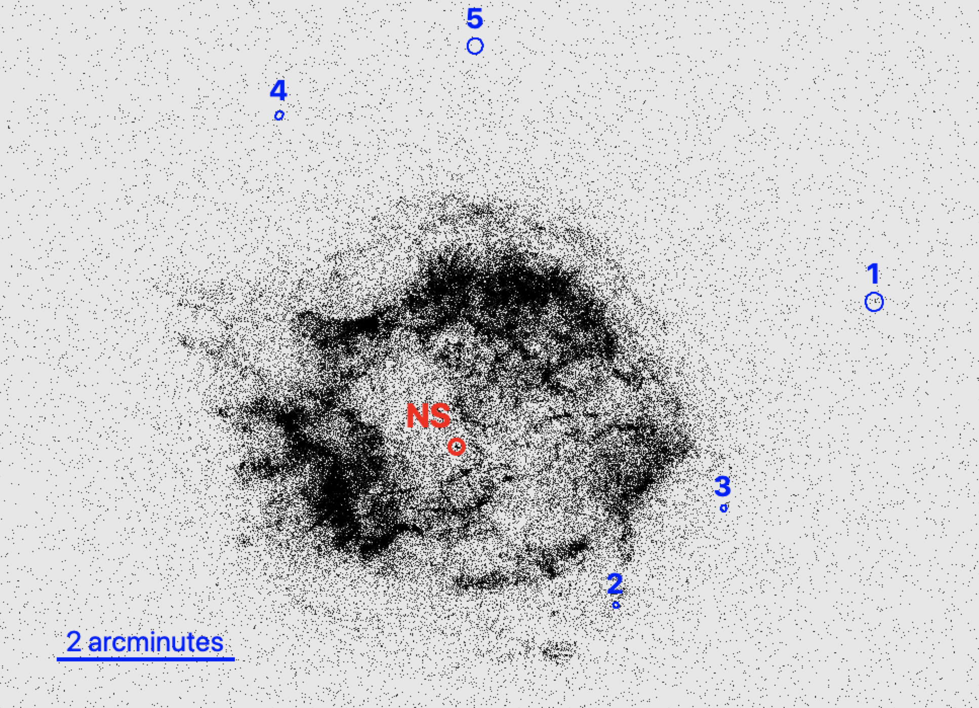
Figure 1: A Chandra image of Cas A, labeled with the NS (red) and detected point sources associated with Gaia counterparts (blue). The size of the circle around each point source is proportional to the uncertainty of the centroid position, i.e., how bright and well-resolved the point source is. The circle around the NS is greatly exaggerated for visibility.

2.3 Chandra’s Astrometric Uncertainties

The astrometric solution for any given Chandra image is only accurate to about $\sim$0.5–1.0”, depending on the detector and epoch of observation. To convert these reported values to 1-$\sigma$ individual uncertainties for RA & Dec, we use the Rayleigh distribution formula:

$$CDF=1-e^{-x^{2}/(2\sigma^{2})}$$ (1)

The CDF—the Cumulative Distribution Function—is the reported confidence interval (often 68% or 90%), x is the reported angular circle uncertainty, and $\sigma$ is the 1D 1-$\sigma$ angular uncertainty value we are solving for.

Table 3: Chandra Astrometric Uncertainty

Detector	2D 68% CI	1D 1-$\sigma$
	(arcsec)	(arcsec)
2018-2023
ACIS-S	0.78”	0.52”
ACIS-I	0.65”	0.40”
HRC-S	0.93”	0.62”
HRC-I	0.71”	0.47”

We followed the advice of Lead Flight Director Dr. Tom Aldcroft to model the astrometric uncertainty evolution as a constant of $\sim$0.6” (90% confidence interval) prior to 2010 and linearly increasing to the reported 2018–2023-averaged values (see Table 3). We extrapolate these detector-specific uncertainties from 1999–2023, setting the individual detector values in 2010 to a factor of 0.6/1.11 smaller since the average 90% confidence interval for 2021 is $\sim$1.11”.

2.4 PSF Modeling and Fitting

To obtain astrometric corrections for each observation, we first needed to obtain precise point source positions that took the detector PSF into account. For this, we followed the methods of past papers (e.g., Mayer et al. 2020; Long et al. 2022). We produce PSF simulations using the CIAO Chandra Ray Tracer (ChaRT) tool, generating five iterations of each point source with a monochromatic spectrum of 1 keV with 0.01 photons cm^-2 s^-1. Most of our point sources are too faint for a robust spectrum to be extracted and modeled, and previous papers (e.g., Long et al. 2022) determined that using a model fit to the extracted spectrum didn’t significantly improve the fits over using this simple spectrum. We then reprocessed those ChaRT output rayfiles using the CIAO tool simulate_psf, which ran them through MARX and generated event files. We binned the resulting event files—HRC observations by 1/2 and ACIS observations by 1/8—to produce final pixel sizes of $\sim$0.065.

After obtaining the PSF files, we followed the steps in the “‘Accounting for PSF Effects in 2D Image Fitting”’ CIAO Sherpa (Freeman et al., 2001) thread to fit each point source using a Gaussian and a constant background and the PSF as the convolution kernel. For each point source in each observation, we obtained a best-fit centroid position along with uncertainties. Using the reported Gaia point source positions and proper motions, we evolved each point source from its 2016 Gaia position to the location it would be at in each Chandra observation. As Gaia point source uncertainties are small ($\lesssim$0.001”), we treated these positions as the “true” reference locations for our calibration point sources.

2.5 Registration Method

At this point, we had robust estimates of calibration point source centroids along with precise reference locations from Gaia for each observation. The next step was to correct the astrometry of each Chandra observation by solving for a transformation matrix such that, when applied to our observations, the identified point sources have positions as close as possible to the reported Gaia positions. The generic transformation matrix is given by

$$\begin{pmatrix}x^{\prime}\\ y^{\prime}\end{pmatrix}=\begin{pmatrix}{\rm r}\cos\theta&-{\rm r}\sin\theta\\ {\rm r}\sin\theta&{\rm r}\cos\theta\end{pmatrix}\begin{pmatrix}x\\ y\end{pmatrix}+\begin{pmatrix}t_{1}\\ t_{2}\end{pmatrix}$$ (2)

where (x,y) are input pixel coordinates of point sources, (x’,y’) are the transformed coordinates, r represents a linear stretching of the image, $\theta$ is rotation, and (t₁,t₂) represents translations. We restricted our transformation matrix to only allow for translation shifts, as the plate scale is well-known and feasible rotation errors will produce small positional changes (0.1^∘ roll angle error corresponds to only a 0.1” shift for sources 1’ away) relative to the $\sim$0.5” astrometric uncertainty. Additionally, some of our images only had 1 or 2 calibration point sources, not enough to find a solution to a full transformation matrix that allowed rotation and/or stretching.

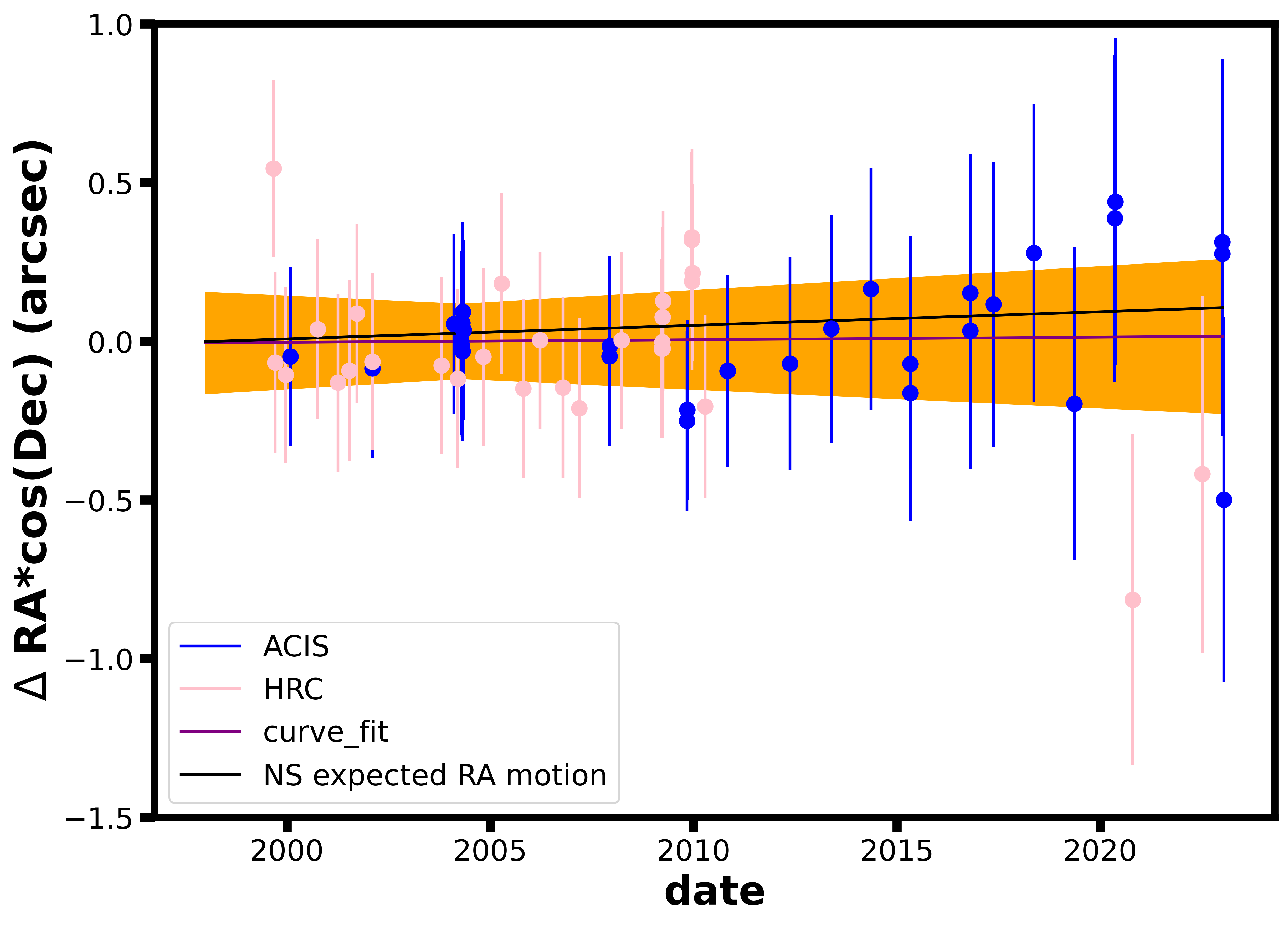
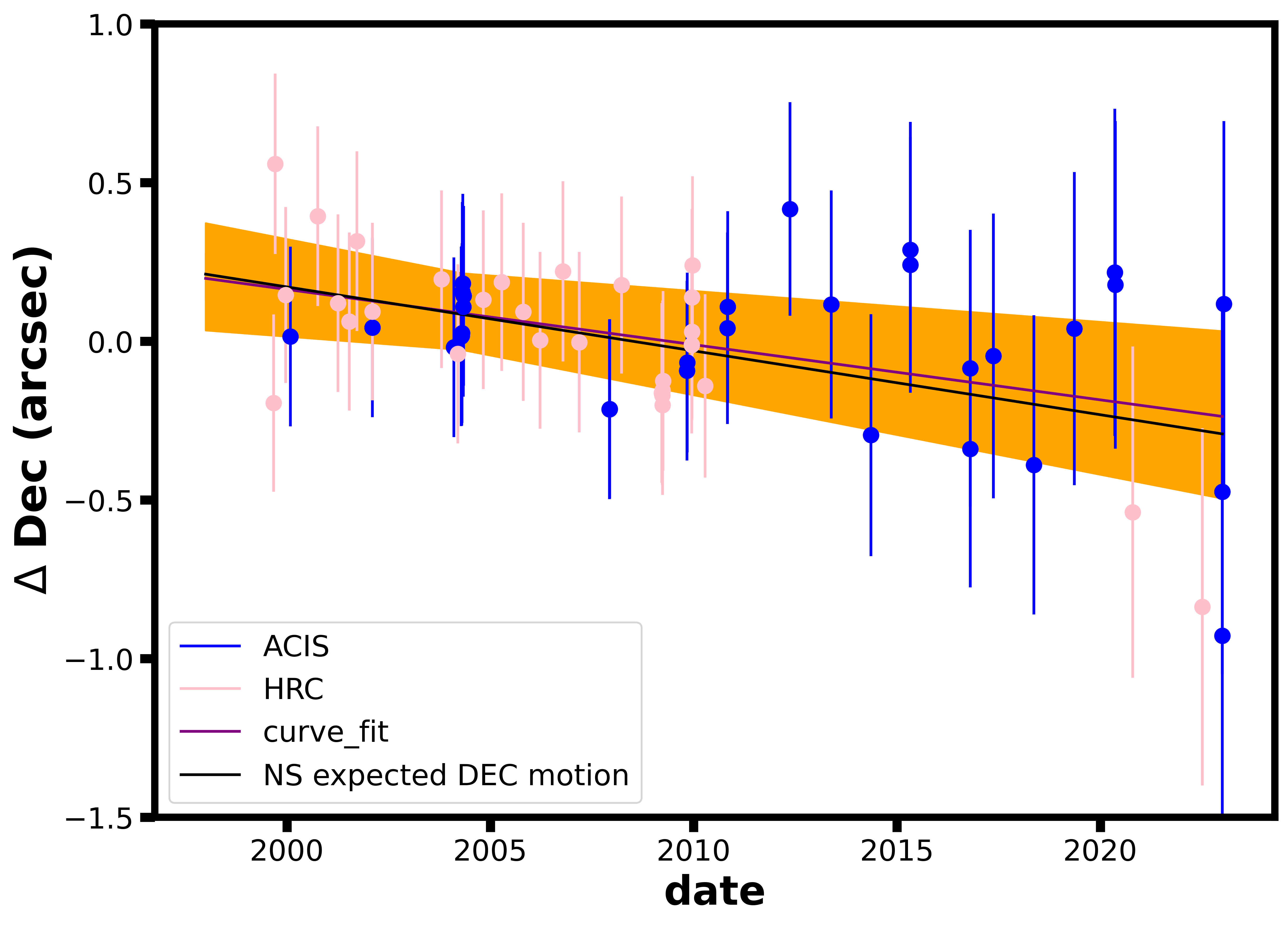
Figure 2: The measured RA & Dec offsets of the Cas A CCO from the average position. The 32 blue points are from ACIS observations and the 29 pink points are from HRC observations. The error bars on each data point reflect the 1-$\sigma$ total uncertainty (wavdetect $+$ astrometric). The green line shows the expected NS motion based on the measurement by Thorstensen et al. (2001), extrapolated from combined 2004 observations. The magenta line shows the best-fit motion, and the orange curve shows the 1-$\sigma$ likelihood region for the line of best-fit, including uncertainty in both slope and intercept and taking the average 2004 NS location as the reference point.

We used a least squares algorithm (Python function scipy.optimize.least_squares) to solve for the transformation matrix, weighting each point source by its centroid uncertainty. Specifically, we used the ‘soft_l1’ loss function option (as in Long et al. 2022) that weights outliers with a linear rather than a quadratic penalty. After obtaining the best-fit translation shifts for each observation, we calculated corrected NS positions by shifting the NS positions (also found via 2D fitting the observation convolved with the PSF) by those values.

2.6 Uncertainties on Final NS Positions

There are three sources of error to combine in quadrature: 1.) the best-fit centroid uncertainty of the NS, 2.) the overall uncertainty of the point sources used to calculate the astrometric solution, and 3.) the accuracy of the astrometric solution. The Gaia point source uncertainties are negligible compared to the point source and astrometric correction uncertainties ($\lesssim$0.001” compared to $\gtrsim$0.05”).

The first uncertainty is simply reported by the process of fitting the point source centroid, as described in Section 2.4. The second and third sources of error result from our decision to weight each point source by its centroid uncertainties when calculating the transformation matrix. As the final translation shift is effectively a weighted average, the uncertainty of the transformation shifts is calculated by adding the inverse centroid errors in quadrature:

$$\sigma_{\rm PSs,tot}=\left(\frac{1}{\sum_{i}^{N}(1/\sigma_{i}^{2})}\right)^{0.5}$$ (3)

We calculate this error separately for both RA & Dec positions.

Finally, the accuracy of the final transformed image—the registration error—is calculated as a weighted average of the differences between the corrected point source locations and their expected Gaia positions (d), using the calibration point sources’ centroid uncertainties as the weights:

$$\sigma_{\rm Res,tot}=\frac{\sum_{i}^{N}(d/\sigma_{i}^{2})}{\sum_{i}^{N}(1/\sigma_{i}^{2})}$$ (4)

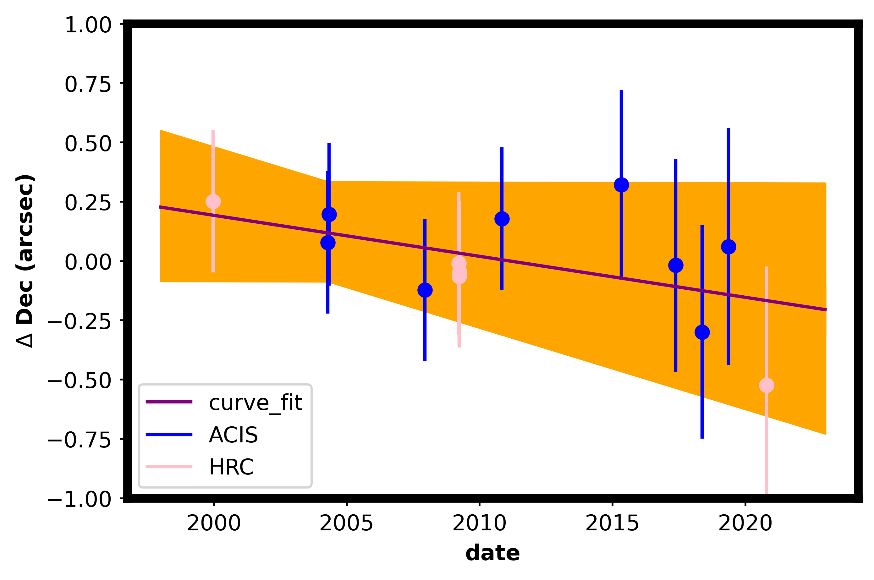
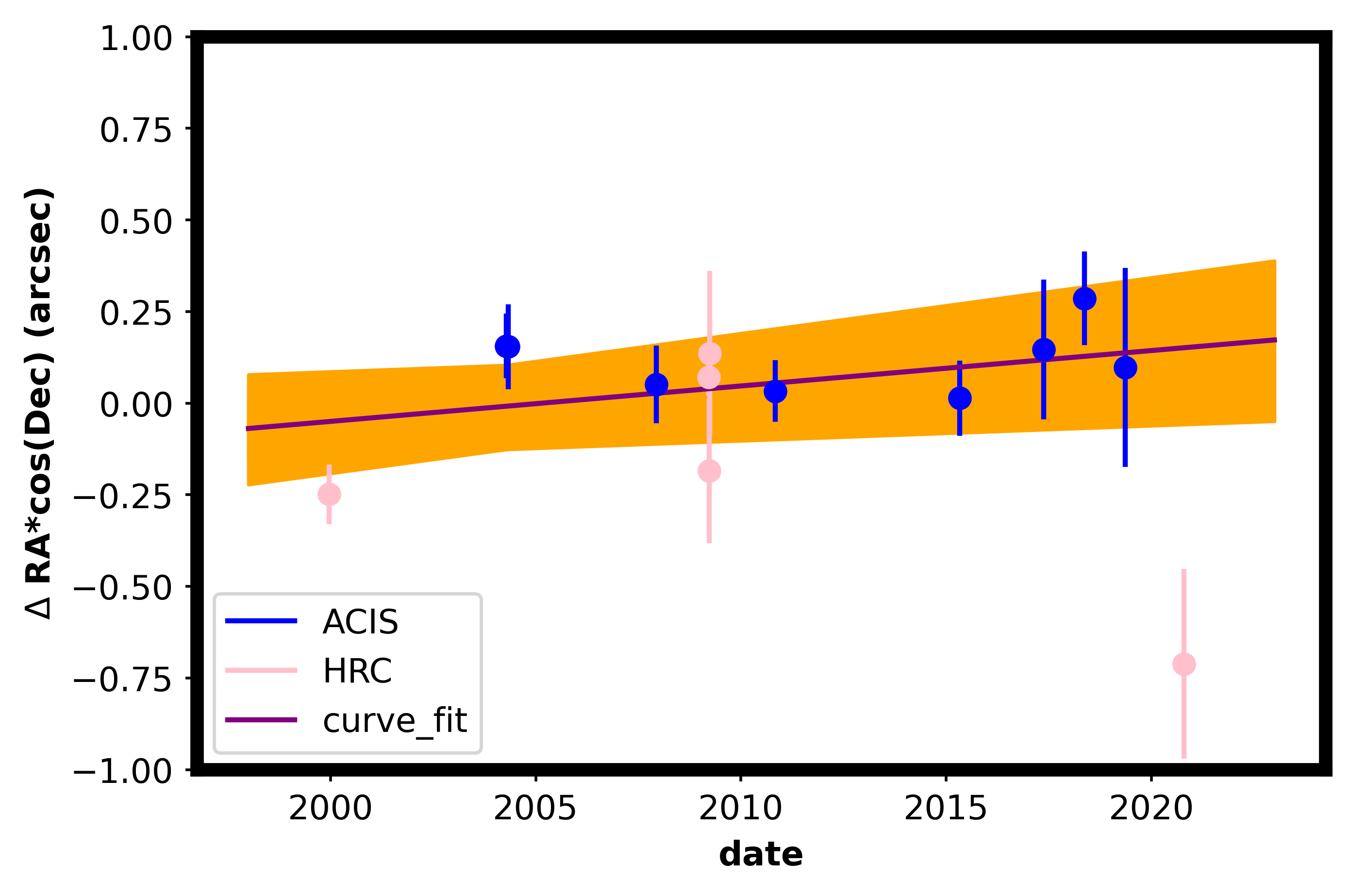
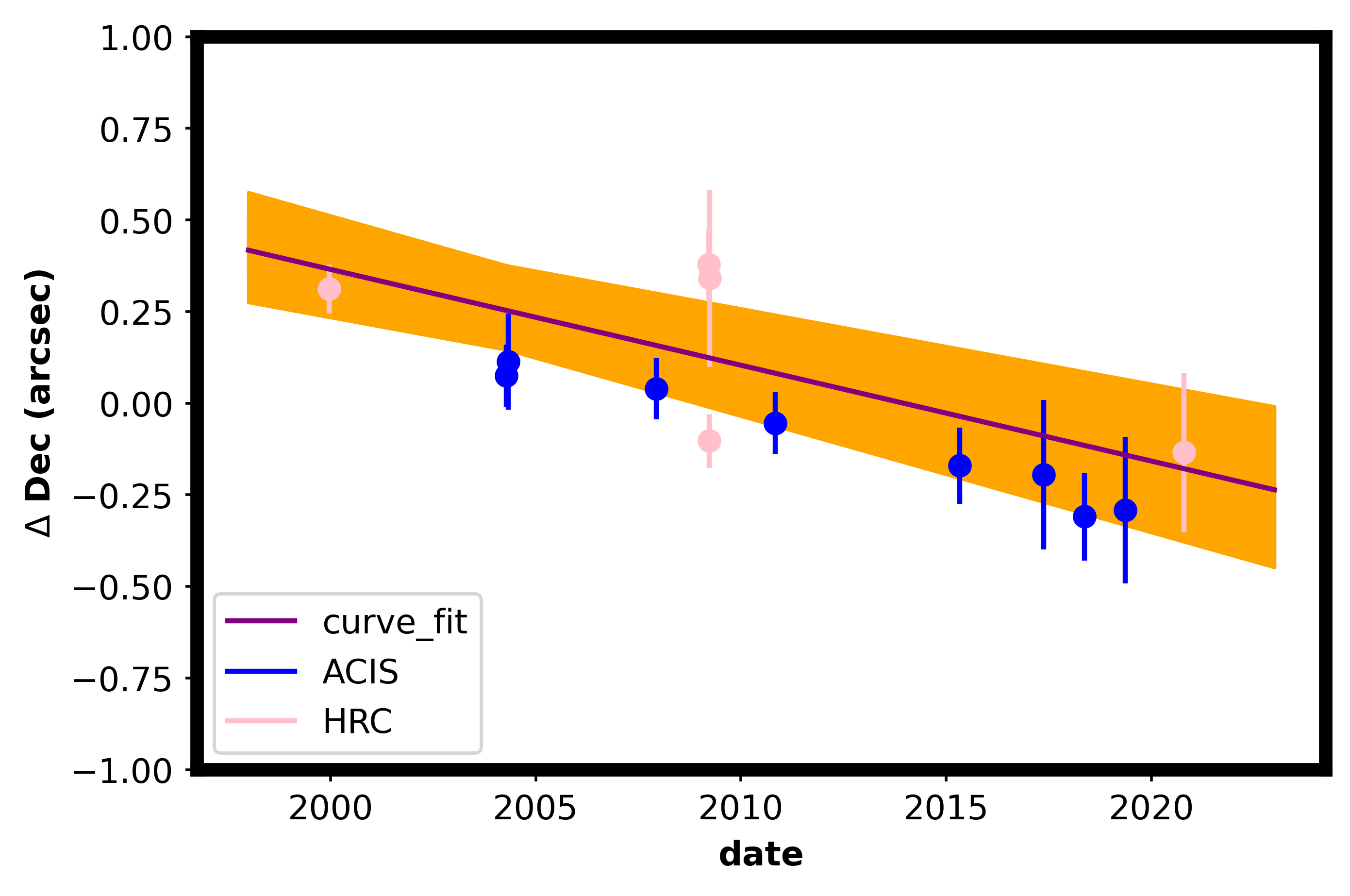
Figure 3: The measured RA & Dec offsets of the Cas A CCO from the average position using the 13 observations with identified calibration point sources. Top) no astrometric correction, Bottom) weighted astrometric correction. The magenta line shows the best fit motion, and the orange curve shows the 1-$\sigma$ likelihood region for the line of best-fit, including uncertainty in both slope and intercept and taking the average uncorrected 2004 NS location as the reference point.

3 Proper Motion of the NS

3.1 Simple Method: All Observations

In the so called “Simple Method” we simply add the expected detector astrometric uncertainty (as estimated in Section 2.3) to the reported best-fit centroid uncertainties of the NS at each epoch. We plot the NS locations measured from 32 ACIS and 29 HRC observations across 24 years and use scipy.optimize.curve_fit in Python to perform non-linear least squares fitting to calculate the RA and Dec motion of the NS. .

We obtained the following proper motion measurements. RA: 0.8 $\pm$ 6.7 mas/yr; Dec: -17.4 $\pm$ 7.7 mas/yr. At a distance of 3.33 kpc, this corresponds to a final velocity of 280 km s^-1 $\pm$ 123 km s^-1, with an angle 87 $\pm$ 22 degrees south of east. The data and lines of best fit are shown in the top row of Figure 2.

3.1.1 Simple Method Check

To double check that our simple method is appropriate for use on Chandra data, we perform the same analysis on a well-known bright star that has many Chandra observations over the years and a robust Gaia proper motion measurement: AR Lac. We extracted the position of AR Lac in 34 Chandra HRC-I observations, applied the astrometric uncertainty to each of the data points, and calculated the line of best fit.

We obtained a measured motion for AR Lac of RA: -57 $\pm$ 8 mas/yr and Dec: 41 $\pm$ 8 mas/yr. The Gaia-reported proper motion is -52.31 $\pm$ 0.02 mas/yr in RAcos(Dec) and 46.83 $\pm$ 0.02 mas/yr in Dec. These results are within 1-$\sigma$ of each other, indicating that this technique of using dozens of Chandra images across multiple decades can enable the accurate measurement of point source proper motions.

3.2 Astrometry-corrected Results

Using our astrometric correction method on the 13 observations, we find a final RA motion of 10.4 $\pm$ 5.6 mas/yr and a final Dec motion of -25.6 $\pm$ 5.6 mas/yr. At a distance of 3.33 kpc, this corresponds to a total velocity of 445 $\pm$ 90 km s^-1 at an angle of 68 $\pm$ 12 degrees south of east. Figure 3 presents the NS positions from these 13 observations, showing proper motions calculated both without and with astrometric corrections.

4 Discussions and Conclusions

In this paper, we have taken advantage of the greater-than-two-decades’ worth of Chandra observations to measure the proper motion of the neutron star in Cassiopeia A. Using a straightforward method that doesn’t correct for astrometric uncertainty but simply accounts for it as an added uncertainty on the NS position across 61 ACIS and HRC Chandra observations, we find a proper motion corresponding to a velocity of 280 km s^-1 $\pm$ 123 km s^-1, with an angle 87 $\pm$ 22 degrees south of east for a distance of 3.33 kpc. Using a more complicated method where we correct 13 observations’ astrometric solutions via associating detected point sources with known Gaia sources, we obtain a velocity of 445 $\pm$ 90 km s^-1 at an angle of 68 $\pm$ 12 degrees south of east.

Our results are separated by 1.08-$\sigma$ and both are within $\sim$1-$\sigma$ of the back-evolved explosion site velocity of $\sim$340 $\pm$ 30 km s^-1 (Thorstensen et al., 2001) and the 570 $\pm$ 260 km s^-1 proper motion measurement using a baseline of 10–years (Mayer & Becker, 2021). The uncertainties of our estimates are smaller by a factor of 2–3 which we attribute to the longer baseline and use of more observations.

Additionally, both of our results produce smaller velocity estimates than found previously. Our astrometry-uncorrected estimate excludes velocities $>$597 km s^-1 at 99% confidence ($\gtrsim$482 km s^-1 at 90% confidence), and our astrometry-corrected estimate excludes velocities $>$677 km s^-1 at 99% confidence ($\gtrsim$593 km s^-1 at 90% confidence). This phenomenon, where velocity estimates are revised to lower velocities when using longer baselines, has been found in proper motion studies of other SNR-embedded NSs. For example, with a 5-year Chandra baseline, the NS in Puppis A was measured to have a velocity of 1,122 $\pm$ 360 km s^-1 (Hui & Becker, 2006) or $\sim$1,600 km s^-1 (Winkler & Petre, 2007). With a $\sim$19 year baseline, this measurement was brought down to 763 $\pm$ 63 km s^-1 (Mayer et al., 2020). We attribute this to the small sky motions—close to zero arcseconds per year—of NSs compared to pixel sizes, telescope astrometry, and other sources of uncertainty. Thus, measurements with short baselines become dominated by any uncertainties or systematic offsets and can become biased away from zero. Determining the true fraction of SNR-embedded NSs with velocities of $\gtrsim$1000 km s^-1 is essential for informing simulations and properly understanding explosion processes in SNe, and this trend suggests that we should be cautious in treating extremely high NS velocities as accurate unless long baselines are used and astrometric uncertainties are properly accounted for.

Finally, our proper motion measurements support previous studies on the relation between NS kick and the properties of the Cas A supernova. The magnitude of our measured kick velocity matches with the 460 km s^-1 values reproduced in Cas A simulations by (Wongwathanarat et al., 2017) using their “Gravitational-Tugboat Mechanism” where the NS is accelerated due to gravitational forces from asymmetric ejecta. Our estimated direction is opposite the bulk of ejecta (Holland-Ashford et al., 2017; Katsuda et al., 2018), and specifically the heaviest ejecta elements Grefenstette et al. (2014); Wongwathanarat et al. (2017); Holland-Ashford et al. (2020); Picquenot et al. (2021), confirming the observational findings of past studies.

Our uncertainty is dominated by the later-epoch ACIS and HRC observations. In particular, the 2020 HRC observation #24840 was only 14 ks which—in combination with the effective area degradation of Chandra at low energies—led to only a single detected calibration point source. In fact, three of the four observations taken after 2016 (ObsIDs #19604, 19606, and 24840) only have a single detected calibration point source. As shown in Figures 2 and 3, the RA of the NS in observation #24840 observation is a notable outlier. We note that there is currently a 35 ks Chandra HRC proposal for this NS waiting to be taken, proposed for by Dr. Heinke. If this observation occurs and multiple Gaia point sources are detected, a more precise proper motion measurement could be made.

Finally, future X-ray telescopes with $\sim$arcsecond precision would greatly help constrain the velocity of this, and other, NSs associated with SNRs. Observations in the 2030s with such an instrument would provide a 30-year baseline compared to early Chandra observations, and in particular smaller off-axis PSFs would enable easier and more precise detections of fore- and background point sources with which to correct image astrometry. In the existing observations of Cas A, we were unable to detect nearby point sources $\gtrsim$3’ off-axis in ACIS observations, and similarly-distant point sources in HRC observations had large centroid uncertainties of up to $\sim$0.5”.

It has been shown—through this study and others—that point source centroid uncertainties smaller than the pixel size or PSF of a detector can be obtained. Thus, even telescopes with up to a few arcsecond spatial resolution should be sufficient to measure NS positions with sufficiently long, multi-decade baselines. The potential probe mission AXIS, the future proposed missions Athena and/or Lynx, and other X-ray telescopes with less than a couple arcsecond resolution are vital to continue our investigations of NS velocities. Until then, continued Chandra observations of select targets (e.g., G11.2-0.3, G18.9-1.1, Cas A, MSH 11-62, and RCW 103) that were observed in the 2000s can enable astronomers to expand the population of SNR-embedded NSs with robust proper motion measurements.

References

- Alarie et al. (2014) Alarie, A., Bilodeau, A., & Drissen, L. 2014, MNRAS, 441, 2996
- Arnaud (1996) Arnaud, K. A. 1996, in Astronomical Society of the Pacific Conference Series, Vol. 101, Astronomical Data Analysis Software and Systems V, ed. G. H. Jacoby & J. Barnes, 17
- Auchettl et al. (2015) Auchettl, K., Slane, P., Romani, R. W., et al. 2015, ApJ, 802, 68
- Babusiaux et al. (2023) Babusiaux, C., Fabricius, C., Khanna, S., et al. 2023, A&A, 674, A32
- Banovetz et al. (2021) Banovetz, J., Milisavljevic, D., Sravan, N., et al. 2021, ApJ, 912, 33
- Becker (2009) Becker, W. 2009, in Astrophysics and Space Science Library, Vol. 357, Astrophysics and Space Science Library, ed. W. Becker, 91
- Bhalerao et al. (2019) Bhalerao, J., Park, S., Schenck, A., Post, S., & Hughes, J. P. 2019, ApJ, 872, 31
- Burke et al. (2021) Burke, D., Laurino, O., wmclaugh, et al. 2021, sherpa/sherpa: Sherpa 4.13.0, doi:10.5281/zenodo.4428938
- Chatterjee et al. (2005) Chatterjee, S., Vlemmings, W. H. T., Brisken, W. F., et al. 2005, ApJ, 630, L61
- Chevalier & Kirshner (1978) Chevalier, R. A., & Kirshner, R. P. 1978, ApJ, 219, 931
- DeLaney & Satterfield (2013) DeLaney, T., & Satterfield, J. 2013, arXiv e-prints, arXiv:1307.3539
- Fesen et al. (2006) Fesen, R. A., Hammell, M. C., Morse, J., et al. 2006, ApJ, 636, 859
- Freeman et al. (2001) Freeman, P., Doe, S., & Siemiginowska, A. 2001, in Society of Photo-Optical Instrumentation Engineers (SPIE) Conference Series, Vol. 4477, Astronomical Data Analysis, ed. J.-L. Starck & F. D. Murtagh, 76–87
- Fruscione et al. (2006) Fruscione, A., McDowell, J. C., Allen, G. E., et al. 2006, in Society of Photo-Optical Instrumentation Engineers (SPIE) Conference Series, Vol. 6270, Society of Photo-Optical Instrumentation Engineers (SPIE) Conference Series, ed. D. R. Silva & R. E. Doxsey, 62701V
- Fryer & Kusenko (2006) Fryer, C. L., & Kusenko, A. 2006, ApJS, 163, 335
- Gaia Collaboration et al. (2016) Gaia Collaboration, Prusti, T., de Bruijne, J. H. J., et al. 2016, A&A, 595, A1
- Gaia Collaboration et al. (2023) Gaia Collaboration, Vallenari, A., Brown, A. G. A., et al. 2023, A&A, 674, A1
- Gessner & Janka (2018) Gessner, A., & Janka, H.-T. 2018, ApJ, 865, 61
- Grefenstette et al. (2014) Grefenstette, B. W., Harrison, F. A., Boggs, S. E., et al. 2014, Nature, 506, 339
- Halpern & Gotthelf (2010) Halpern, J. P., & Gotthelf, E. V. 2010, ApJ, 709, 436
- Hobbs et al. (2005) Hobbs, G., Lorimer, D. R., Lyne, A. G., & Kramer, M. 2005, MNRAS, 360, 974
- Holland-Ashford et al. (2020) Holland-Ashford, T., Lopez, L. A., & Auchettl, K. 2020, ApJ, 889, 144
- Holland-Ashford et al. (2017) Holland-Ashford, T., Lopez, L. A., Auchettl, K., Temim, T., & Ramirez-Ruiz, E. 2017, ApJ, 844, 84
- Hughes et al. (2000) Hughes, J. P., Rakowski, C. E., Burrows, D. N., & Slane, P. O. 2000, ApJ, 528, L109
- Hui & Becker (2006) Hui, C. Y., & Becker, W. 2006, A&A, 457, L33
- Igoshev (2020) Igoshev, A. P. 2020, MNRAS, 494, 3663
- Janka (2017) Janka, H.-T. 2017, ApJ, 837, 84
- Johnston et al. (2005) Johnston, S., Hobbs, G., Vigeland, S., et al. 2005, MNRAS, 364, 1397
- Katsuda et al. (2018) Katsuda, S., Morii, M., Janka, H.-T., et al. 2018, ApJ, 856, 18
- Lai (2001) Lai, D. 2001, in Lecture Notes in Physics, Berlin Springer Verlag, Vol. 578, Physics of Neutron Star Interiors, ed. D. Blaschke, N. K. Glendenning, & A. Sedrakian, 424
- Long et al. (2022) Long, X., Patnaude, D. J., Plucinsky, P. P., & Gaetz, T. J. 2022, ApJ, 932, 117
- Mayer et al. (2020) Mayer, M., Becker, W., Patnaude, D., Winkler, P. F., & Kraft, R. 2020, ApJ, 899, 138
- Mayer & Becker (2021) Mayer, M. G. F., & Becker, W. 2021, A&A, 651, A40
- Picquenot et al. (2021) Picquenot, A., Acero, F., Holland-Ashford, T., Lopez, L. A., & Bobin, J. 2021, A&A, 646, A82
- Rest et al. (2011) Rest, A., Foley, R. J., Sinnott, B., et al. 2011, ApJ, 732, 3
- Scheck et al. (2006) Scheck, L., Kifonidis, K., Janka, H.-T., & Müller, E. 2006, A&A, 457, 963
- Shternin et al. (2019) Shternin, P., Kirichenko, A., Zyuzin, D., et al. 2019, ApJ, 877, 78
- Tananbaum (1999) Tananbaum, H. 1999, IAU Circ., 7246, 1
- Temim et al. (2017) Temim, T., Slane, P., Plucinsky, P. P., et al. 2017, ApJ, 851, 128
- Thorstensen et al. (2001) Thorstensen, J. R., Fesen, R. A., & van den Bergh, S. 2001, AJ, 122, 297
- Verbunt & Cator (2017) Verbunt, F., & Cator, E. 2017, Journal of Astrophysics and Astronomy, 38, 40
- Winkler & Petre (2007) Winkler, P. F., & Petre, R. 2007, ApJ, 670, 635
- Winkler et al. (2009) Winkler, P. F., Twelker, K., Reith, C. N., & Long, K. S. 2009, ApJ, 692, 1489
- Wongwathanarat et al. (2013) Wongwathanarat, A., Janka, H.-T., & Müller, E. 2013, A&A, 552, A126
- Wongwathanarat et al. (2017) Wongwathanarat, A., Janka, H.-T., Müller, E., Pllumbi, E., & Wanajo, S. 2017, ApJ, 842, 13