Detectable MeV Neutrino Signals from Neutron-Star Common-Envelope Systems

Abstract

Common-envelope evolution — where a star is engulfed by a companion — is a critical but poorly understood step in, e.g., the formation pathways for gravitational-wave sources. However, it has been extremely challenging to identify observable signatures of such systems. We show that for systems involving a neutron star, the hypothesized super-Eddington accretion onto the neutron star produces MeV-range, months-long neutrino signals within reach of present and planned detectors. While there are substantial uncertainties on the rate of such events (0.01–1/century in the Milky Way) and the neutrino luminosity (which may be less than the accretion power), this signal can only be found if dedicated new searches are developed. If detected, the neutrino signal would lead to significant new insights into the astrophysics of common-envelope evolution.

What happens when an ordinary star engulfs a neutron star? While this sounds exotic, it is believed to happen relatively frequently (0.01–1 /century in the Milky Way) in binary and higher-multiplicity star systems, and is an especially interesting example of common-envelope evolution Paczynski:1976 ; Han:1995 ; Belczynski:2016 ; Fragos:2019box ; Ivanova:2013 ; Ivanova:2020 ; Ginat:2019qvu ; Hutilukejiang:2018 . For instance, it is considered necessary to explain the existence of X-ray binaries and gravitational-wave sources involving neutron stars. Both types of objects require extremely tight binary systems that may be produced through common-envelope evolution. But the process itself is mysterious because it is very difficult to tell if a star is harboring a neutron star.

Inside a host star, a neutron star is expected to accrete material at a high rate due to its strong gravitational field and the large ambient density. The process ends when the neutron star merges with the core of the host star or when the envelope is blown off. However, the details are poorly understood. If outward radiation pressure counterbalances gravity, accretion is stabilized at the so-called Eddington limit, and gravitational energy is converted into photons. Yet since the early 1990s it has been argued that accretion can become so fast that radiation is trapped and pulled inward, leading to super-Eddington (hypercritical) accretion rates Chevalier:1989 ; Houck:1991 ; Chevalier:1993 ; Ricker:2012 ; MacLeod:2014yda ; MacLeod:2017 ; Fragos:2019box . In this case, the accretion flow would heat up to the point where neutrino emission becomes the dominant cooling channel, as illustrated in Fig. 1.

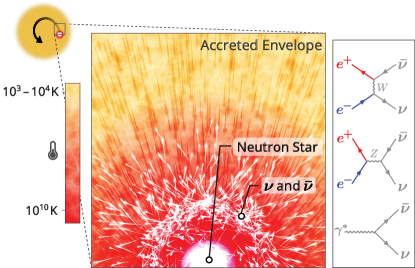
Figure 1: Neutrino production via super-Eddington accretion onto a neutron star in a common-envelope system. Infalling matter releases gravitational potential energy and heats up until cooling via neutrino emission becomes dominant.

In this Letter, we investigate this neutrino emission. We show that months-long super-Eddington accretion rates of up to $\dot{M}\simeq$0.1\text{\,}\mathrm{M}_{\odot}\,\mathrm{y}\mathrm{r}^{-1}$$, as predicted by several simulations Houck:1991 ; Chevalier:1993 ; Ricker:2012 ; Ivanova:2013 ; MacLeod:2014yda ; MacLeod:2017 ; Ivanova:2020 , imply a flux of MeV neutrinos that, for a system in the Milky Way, is observable in current and upcoming detectors like Super-Kamiokande, JUNO, and DUNE. Discovery would require dedicated analyses, as well as some amount of luck given the low anticipated rate of galactic common-envelope events. Without a search, we will definitely miss a neutrino signal that would provide direct answers to many of the most important questions surrounding common-envelope evolution, such as the accretion rate, duration, and outcome. Once a discovery has been made, the key observable will be the time profile of the emission. For close sources, crude directionality will also be possible.

In the following, we describe the astrophysics of neutron star common-envelope systems; then calculate the neutrino flux, spectrum, and detection prospects; and, last, conclude and discuss directions for future work. In the Supplemental Material, which includes Refs. Shapiro:1973 ; Cox_Giuli ; Bildsten:1998km ; Egawa:1977 ; Paxton2011 ; Paxton2013 ; Paxton2015 ; Paxton2018 ; Paxton2019 ; Jermyn2023 ; Rogers2002 ; Saumon1995 ; Irwin2004 ; Timmes2000 ; Potekhin2010 ; Itoh:1996 ; Clark:2022tli ; MacLeod:2015 ; Landau:1959 ; Kato:2015faa ; Dighe:1999bi ; Kuo:1989qe ; Maltoni:2015kca ; Esteban:2020cvm ; Brdar:2023ttb ; Vogel:1999zy ; Strumia:2003zx ; Super-Kamiokande:2016yck ; JUNO:2023vyz ; JUNO:2015zny ; Formaggio:2012cpf ; Castiglioni:2020tsu , we provide technical details on our simulations and results.

Astrophysical framework.— We review common-envelope evolution with a neutron star (for details, see, e.g., Refs. Iben:1993yi ; Ivanova:2020 ; Roepke:2022icg ). The process starts when the host star overfills its Roche lobe, either because it expands or because the orbital separation decreases. The neutron star inspirals within the host’s envelope due to drag, accreting material at potentially high rates due to the large ambient density. The duration of this phase is limited to a time $\sim\mathrm{month}\times($0.1\text{\,}\mathrm{M}_{\odot}\mathrm{/}\mathrm{y}\mathrm{r}$/\dot{M})$ Iben:1993yi ; MacLeod:2014yda , and possible outcomes include envelope ejection or core merger (forming a Thorne–Żytkov object) Thorne:1977 ; Houck:1991 ; Fryer:1995dr ; Popham:1998ab ; Brown:1999dda ; Narayan:2001 ; Lee:2005se ; Lee:2005et .

If the mass accretion rate onto the neutron star is low, gravitational potential energy is primarily released as electromagnetic radiation. In this regime, accretion cannot exceed the Eddington rate, $\sim${10}^{-8}\text{\,}\mathrm{M}_{\odot}\mathrm{/}\mathrm{y}\mathrm{r}$$ for a neutron star Houck:1991 , as radiation pressure hinders further accretion. However, stable super-Eddington accretion is possible if the inflow velocity is large enough to trap radiation. The primary energy loss process is then thermal neutrino emission Houck:1991 ; Chevalier:1993 . This is thought to occur for accretion rates above $\sim${10}^{-4}\text{\,}\mathrm{M}_{\odot}\mathrm{/}\mathrm{y}\mathrm{r}$$, though there are significant uncertainties Ricker:2012 ; Ivanova:2013 ; Fragos:2019box , partly due to numerical challenges Roepke:2022icg . One uncertainty regards the need to dissipate angular momentum, but super-Eddington rates as large as $0.1\text{\,}\mathrm{M}_{\odot}\mathrm{/}\mathrm{y}\mathrm{r}$ are found in simulations both neglecting Houck:1991 ; Brown:1995 and including this effect Brown:1999dda ; Ricker:2012 ; MacLeod:2014yda ; MacLeod:2017 . Another is whether all energy is dissipated by neutrino emission or whether other mechanisms such as jet formation play an important role MorenoMendez:2017xmw ; Murguia-Berthier:2017 ; Chamandy:2018 ; Lopez-Camara:2018cym ; Lopez-Camara:2020pot ; MorenoMendez:2022obo . Moreover, transitioning from sub-Eddington ($\lesssim 10^{-8}M_{\odot}/\mathrm{yr}$) to steady-state super-Eddington ($\gtrsim 10^{-4}M_{\odot}/\mathrm{yr}$) rates requires departures from steady-state spherical accretion, with the details being uncertain Chevalier:1993 ; Houck:1991 ; Sakurai:2016hns ; Sugimura:2016dmy .

The frequency of neutron-star common-envelope events in the Milky Way is uncertain. An upper bound is the supernova rate, roughly $\sim 1$/century Rozwadowska:2020nab (neutron stars are not born frequently enough to sustain higher common-envelope rates), while a lower bound is the theoretically estimated formation rate of Thorne–Żytkov objects, roughly $0.01$/century Hutilukejiang:2018 ; Podsiadlowski:1995 . Refs. Hutilukejiang:2018 ; Ginat:2019qvu estimate a neutron-star common-envelope rate of roughly $0.1$/century.

Neutrino flux.— We first make a simple estimate of the neutrino emission rate for super-Eddington accretion, then describe detailed calculations that support it.

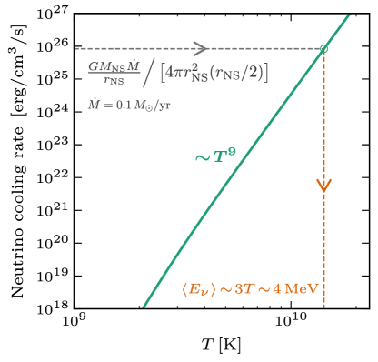
Figure 2: Energy emission in neutrinos as a function of temperature (solid). Due to the steep dependence, the average neutrino energy is robustly determined from the gravitational energy release rate due to accretion (horizontal dashed).

Figure 2 shows that the average neutrino energy, $\langle E_{\nu}\rangle$, is large enough to be detectable. It is similar to the energies of the electrons, positrons, and plasmons from which neutrinos are dominantly produced Itoh:1996 , $\langle E_{\nu}\rangle\sim 3T\sim$4\text{\,}\mathrm{M}\mathrm{e}\mathrm{V}$$, with $T$ the temperature of the accretion flow. $T$ is simply but robustly determined by equating the rate of gravitational potential energy release to the neutrino cooling rate. For the gravitational energy release, we assume $\dot{M}=$0.1\text{\,}\mathrm{M}_{\odot}\mathrm{/}\mathrm{y}\mathrm{r}$$, a neutron star of mass $M_{\text{NS}}=$1.3\text{\,}\mathrm{M}_{\odot}$$ and radius $r_{\text{NS}}=$12\text{\,}\mathrm{k}\mathrm{m}$$. Moreover, we assume that the energy is released in a shell of thickness $r_{\text{NS}}/2$. We follow Refs. Dicus:1972yr ; Braaten:1993jw to compute the neutrino cooling rate, which scales $\propto T^{9}$. Therefore, the specifics of the accretion process hardly matter for determining $\langle E_{\nu}\rangle$.

The overall neutrino flux scales linearly with the accretion rate. For the above parameters, accretion releases $GM_{\mathrm{NS}}\dot{M}/r_{\mathrm{NS}}\simeq${10}^{45}\text{\,}\mathrm{e}\mathrm{r}\mathrm{g}\mathrm{/}\mathrm{s}$$ of gravitational energy. When carried by neutrinos with energies $\sim$4\text{\,}\mathrm{M}\mathrm{e}\mathrm{V}$$, this corresponds to a neutrino production rate $\sim${10}^{50}\text{\,}\mathrm{s}^{-1}$$ or, at a distance of $10\text{\,}\mathrm{k}\mathrm{p}\mathrm{c}$, to a flux $\sim${10}^{4}\text{\,}\mathrm{c}\mathrm{m}^{-2}\mathrm{s}^{-1}$$. Folded with the cross section for inverse beta decay at the relevant energies, $\sim${10}^{-42}\text{\,}\mathrm{c}\mathrm{m}^{2}$$, this corresponds to about a hundred events over a few months in a detector like Super-Kamiokande.

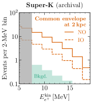
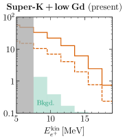
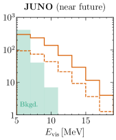
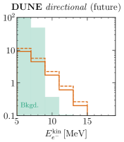
Figure 3: Neutrino signal at different detectors from a super-Eddington neutron-star common-envelope event, integrating over three months (see text for details). Using the astrophysical model from Ref. MacLeod:2014yda , we show the prediction for the normal (NO, solid) and inverted (IO, dashed) mass orderings. Gray regions are below the energy cuts of publicly available background estimates. Super-Kamiokande and JUNO (note the different vertical scales) would detect $\bar{\nu}_{e}$ with high statistics; whereas DUNE could detect neutrino–electron scattering and thereby roughly localize the source. A common-envelope neutrino signal can be detectable in past, present, and future detectors.

To go beyond these simple estimates, we compute the temperature and density profile of the accretion flow by solving the equations of hydrodynamics in a spherical setup, following Refs. Houck:1991 . The accretion rate as a function of time is taken from the simulation in Ref. MacLeod:2014yda , which predicts $\dot{M}\sim${10}^{-3}\text{\,}\mathrm{M}_{\odot}\mathrm{/}\mathrm{y}\mathrm{r}$$ at the onset, increasing to $\sim$0.1\text{\,}\mathrm{M}_{\odot}\mathrm{/}\mathrm{y}\mathrm{r}$$ when the neutron star reaches the core of the host after a few months. We focus on the final three months, during which $\gtrsim 90\%$ of neutrinos are emitted. For a given temperature and density, we compute the neutrino flux from electron–positron annihilation, following Ref. Dicus:1972yr ; and the subdominant flux from plasmon decay, following Ref. Braaten:1993jw . Both processes produce neutrinos of all flavors, with a preference for $\nu_{e}$ and $\bar{\nu}_{e}$. We propagate neutrinos out of the star assuming adiabatic flavor conversion (non-adiabaticities lead to $\lesssim 10\%$ corrections). We also account for gravitational redshift and neutrino absorption by the neutron star Fattoyev:2017ybi . The details of the calculation are given in the Supplemental Material. To support further work, our code is publicly available.

The flavor composition of the emitted neutrino flux depends on the neutrino mass ordering. For the normal ordering, both MSW resonances lie in the neutrino sector. Considering neutrinos and anti-neutrinos that are initially of electron type (the most abundantly produced and easiest to detect flavor), this means that an initial $\nu_{e}$ will leave the star approximately as a $\nu_{3}$ mass eigenstate, with only a $\sim 2\%$ $\nu_{e}$ admixture; and an initial $\bar{\nu}_{e}$ will leave as a $\bar{\nu}_{1}$, which has a sizable ($\sim 70\%$) $\bar{\nu}_{e}$ component. For the inverted ordering, in contrast, there are resonances for neutrinos and antineutrinos, where $\bar{\nu}_{e}$ are almost completely converted to other flavors, while $\nu_{e}$ retain a large electron flavor component.

Neutrino detection.— The most promising detection channels for neutrinos from a common-envelope system are inverse beta decay ($\bar{\nu}_{e}+p\to e^{+}+n$, with a relatively large cross section) and neutrino–electron scattering ($\nu+e^{-}\to\nu+e^{-}$, with some directionality). The main backgrounds are due to spallation induced by cosmic-ray muons Li:2014sea ; Li:2015lxa ; Li:2015kpa ; Zhu:2018rwc ; JUNO:2021vlw , which produces radioactive isotopes, and neutral-current interactions of atmospheric neutrinos Ankowski:2011ei ; T2K:2014vog ; Super-Kamiokande:2019hga ; T2K:2019zqh ; JUNO:2021vlw . For any detectable signal, the average neutrino energy will be fairly independent of the conditions in the source, while the flux normalization will depend on the accretion rate and the source distance. The duration and time profile are key observables, as they will test the astrophysical conditions in the source.

We consider the following detectors (see Supplemental Material for details):

• Super-K (archival). A search for a common-envelope signal using the decades worth of existing Super-Kamiokande data will resemble a search for the diffuse supernova neutrino background Super-Kamiokande:2021jaq , augmented by search criteria exploiting the transient nature of the signal. Such an analysis would benefit from a well-understood detector, though the detection efficiency would be relatively low (5–15%) due to the challenges associated with neutron tagging.

• Super-K (low Gd). The Super-Kamiokande collaboration has recently added a small amount (0.01% mass fraction) of gadolinium to their detector to improve the tagging of neutrons produced in inverse beta decay Beacom:2003nk ; Super-Kamiokande:2023xup . Still, the detection efficiency remains low, 15–30%.

• Super-K (Gd, optim.), an optimistic future upgrade of Super-Kamiokande, with enough gadolinium to increase the detection efficiency to 75% while maintaining the same background levels as in Ref. Super-Kamiokande:2023xup .

• JUNO, a detector concluding construction with a fiducial volume similar to Super-Kamiokande. Filled with liquid scintillator, JUNO’s detection efficiency is large, 73% JUNO:2021vlw . The detector suffers, however, from sizable reactor and spallation backgrounds due to its location.

• Hyper-K, the successor to Super-Kamiokande with an eight times larger fiducial volume. We assume the same detection efficiency as for Super-K (archival), but larger spallation backgrounds due to the detector’s shallower depth Hyper-Kamiokande:2018ofw .

• Hyper-K (Gd), a hypothetical upgrade of Hyper-Kamiokande with gadolinium loading for the same detection efficiency as Super-K (Gd, optim.).

• DUNE, a future liquid argon detector that can detect MeV neutrino–electron scattering. The large solar neutrino background in this channel can be removed by exploiting directionality. Solar $\nu_{e}$ can scatter on ⁴⁰Ar as well, but we first assume that these events can be rejected by identifying final-state $\gamma$ rays from nuclear de-excitation DUNE:2020ypp (for completeness, we later consider the opposite scenario too). The solar neutrino background is why $\nu_{e}$–argon scattering is not a useful detection channel for common-envelope signals.

Figure 3 shows that the neutrino signal from a nearby common-envelope event can be sizable, with the rate well above backgrounds. We use the accretion rates from Ref. MacLeod:2014yda as described above. For models with other values of $\dot{M}$, the spectrum would be very similar, while the normalization would scale $\propto\dot{M}$.

Discovery reach.— Figure 4 (top panel) shows that current and near-future detectors are sensitive to common-envelope events in a large fraction of the Milky Way. We show the maximal distance at which a given experiment can detect a signal with $3\sigma$ significance, assuming normal mass ordering (see Supplemental Material for details and for inverted ordering results). For sources even slightly closer, the significance is much larger because the signal scales as the inverse distance squared. The black line in the plot shows the fraction of Milky Way stars within a given distance from Earth using the thin disk parameters from Refs. Girardi:2005fk ; Adams:2013ana , appropriate for common-envelope host stars Ivanova:2020 . For comparison, supernova neutrino bursts can currently be detected out to hundreds of kpc (which includes the whole Milky Way and potentially the Andromeda galaxy Ando:2005ka ), and pre-supernova neutrino emission out to $1\text{\,}\mathrm{k}\mathrm{p}\mathrm{c}$ Li:2020gaz ; JUNO:2023dnp . Figure 4 (bottom panel) shows the same for searches using neutrino–electron scattering. While these are sensitive only to events in our local neighborhood (out to $2\text{\,}\mathrm{k}\mathrm{p}\mathrm{c}$ at best), they would be able to localize the source in the sky to within about $5\mathrm{°}$ DUNE:2020ypp .

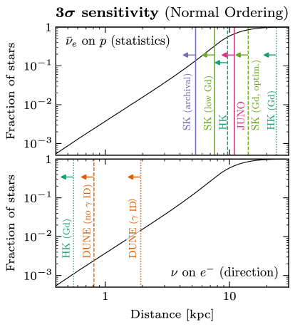
Figure 4: Discovery reach for common-envelope events in the inverse beta decay (top) and neutrino–electron scattering (bottom) channels, using the sizable accretion rates from Ref. MacLeod:2014yda . The black line shows the fraction of Milky Way stars within a given distance from Earth. Current detectors reach a large fraction of the galaxy, and significant improvement is possible. Directionality is more challenging.

Our assumptions on experimental capabilities are conservative, with much room for improvement. The gadolinium concentration in Super-Kamiokande has already been increased to 0.03% Super-Kamiokande:2023xup to increase the detection efficiency. The energy cut could also be lowered, as can be seen in Fig. 3. If the background due to atmospheric-neutrino neutral-current interactions were greatly reduced, the reach of Super-K (Gd, optim.) would change from $14\text{\,}\mathrm{k}\mathrm{p}\mathrm{c}$ to $21\text{\,}\mathrm{k}\mathrm{p}\mathrm{c}$. For both Super-Kamiokande and JUNO, further work on reducing spallation backgrounds Li:2015lxa ; Super-Kamiokande:2021snn could increase the reach by up to $\sim$ 20%. For DUNE, the most important capability is $\gamma$-ray identification; although neutron shielding, as proposed in Refs. Capozzi:2018dat ; Zhu:2018rwc , would further increase the reach by $\sim$ 20%.

Outlook and future directions.— Neutron-star common-envelope events are predicted to occur in the Milky Way at a rate of 0.01–1/century, but it has not been possible to detect them. Here we show that they would release strong, MeV-range neutrino fluxes if accretion onto the neutron star is super-Eddington, as suggested by simple accretion theory and more involved simulations. Importantly, while neutrino fluxes are within reach of present and future detectors, they could have already been missed due to a lack of targeted searches, though this could be fixed even for archival data. This establishes common-envelope systems as a potential third low-energy astrophysical neutrino source, besides supernovae and the Sun.

Just the fact of a successful detection would reveal both that a neutron star is being absorbed by an ordinary star and that super-Eddington accretion is possible. The time evolution of the signal would reveal the dynamics of the inspiraling neutron star. This would be a crucial input for more broadly understanding common-envelope evolution, which remains mysterious because the dense overburden of the envelope shields electromagnetic signals. As an example of a benefit, this would help us understand the pathways that lead to observed gravitational-wave signals from neutron star and black hole mergers.

Identifying the specific star where common-envelope evolution occurs remains a long-term challenge. For a nearby event, the signal from neutrino–electron scattering could potentially localize the event to within about five degrees (comparable to supernova burst detection Beacom:1998fj ), which would be adequate to define a search window for a future electromagnetic outburst if the envelope is ejected. To identify a star before that, some breakthrough is needed in either electromagnetic or gravitational-wave signal detection, as has been suggested in Refs. Ivanova:2013 ; Holgado:2017vut ; Ginat:2019qvu . Ultimately, if such techniques are successful, even the non-observation of neutrinos from an event would be significant, indicating that super-Eddington accretion is not occurring and setting upper limits on the accretion rate and temperature of the accretion flow.

One interesting direction of future work is the details of incorporation of accreted material into the neutron star. Nuclear reactions deprotonize the infalling matter Keegans:2019gje , which leads to an extra flux of MeV-scale neutrinos. This flux will be lower than the one from cooling: a proton gains of order $100\text{\,}\mathrm{M}\mathrm{e}\mathrm{V}$ in energy during infall, which requires tens of $\sim$4\text{\,}\mathrm{M}\mathrm{e}\mathrm{V}$$ neutrinos to dissipate. Nuclear reactions, on the other hand, yield less than one neutrino per infalling proton. The timescale for these nuclear reactions can also be different. Encouragingly, the neutrino flux from deprotonization could be detectable not only from common-envelope events involving neutron stars, but also from those involving white dwarfs, which are far more common. Further explorations are needed.

Acknowledgments.— It is a pleasure to thank Simone Bavera, Tassos Fragos, Iñigo Gonzalez, Matthias Kruckow, Shirley Li, Todd Thompson, and Stephan Meighen-Berger for very useful discussions, and Daniel Dominguez (CERN Design and Visual Identity Team) for preparing Fig. 1. I.E. acknowledges support from Eusko Jaurlaritza (IT1628-22). J.F.B. was supported by National Science Foundation Grant No. PHY-2310018.

Supplemental Material
Detectable MeV Neutrino Signals from Common-Envelope Systems
Ivan Esteban, John F. Beacom, and Joachim Kopp

Here, we provide technical details of our simulations and results to aid further work. We discuss temperature and density profiles during super-Eddington accretion in Section A, neutrino spectra in Section B, neutrino oscillations in Section C, neutrino detection in Section D, and the distance reach in the inverted mass ordering in Section E.

As discussed in the main text, the neutrino flux and average energy are robustly determined by energy conservation. The details discussed in this Supplemental Material allow to sharpen the predictions, but they are not important for our conclusions.

A Hydrodynamic equations

We describe how we compute the temperature and density profile of the accretion flow to obtain the neutrino flux. The procedure largely follows Ref. Houck:1991 . As discussed in the main text, the neutrino flux and average energy follow from energy conservation arguments, and are thus not sensitive to the details of the computation.

As gas is accreted by the neutron star, its evolution is governed by the equations of hydrodynamics. Ref. Chevalier:1989 found that the process can be described by a sequence of steady states. We further assume spherical symmetry Houck:1991 ; Murguia-Berthier:2017 . For the large inflow velocities in super-Eddington accretion, radiation diffusion can be neglected Houck:1991 and the equations for steady-state spherically symmetric accretion including relativistic effects read Houck:1991 ; Shapiro:1973

$$\frac{1}{r^{2}}\frac{\mathop{\mathrm{\mathstrut d}}\nolimits(r^{2}\rho v)}{\mathop{\mathrm{\mathstrut d}}\nolimits\!r} =0\,,$$ (continuity equation) (A1)

$$\frac{\mathop{\mathrm{\mathstrut d}}\nolimits(\rho c^{2}+e)}{\mathop{\mathrm{\mathstrut d}}\nolimits\!r}-\frac{w}{\rho}\frac{\mathop{\mathrm{\mathstrut d}}\nolimits\!\rho}{\mathop{\mathrm{\mathstrut d}}\nolimits\!r} =\frac{\varepsilon_{\mathrm{nuc}}-\mathcal{L}_{\nu}}{v}\,,\qquad$$ (energy conservation) (A2)

$$v\frac{\mathop{\mathrm{\mathstrut d}}\nolimits\!v}{\mathop{\mathrm{\mathstrut d}}\nolimits\!r}+\frac{GM_{\mathrm{NS}}}{r^{2}}+\frac{1}{w}\frac{\mathop{\mathrm{\mathstrut d}}\nolimits\!P}{\mathop{\mathrm{\mathstrut d}}\nolimits\!r}\left(v^{2}+c^{2}-\frac{2GM_{\mathrm{NS}}}{r}\right) =0\,,$$ (Euler equation) (A3)

with $r$ the radial coordinate, $\rho$ the mass density, $v$ the radial component of the fluid four-velocity, $G$ Newton’s constant, $M_{\mathrm{NS}}$ the neutron star mass, $P$ the fluid pressure, $w\equiv\rho c^{2}+e+P$ the relativistic enthalpy, with $e$ the fluid internal energy density and $c$ the speed of light, $\varepsilon_{\mathrm{nuc}}$ the nuclear energy generation rate per unit volume, and $\mathcal{L}_{\nu}$ the energy loss rate per unit volume due to neutrinos. Here $\rho$, $e$, $P$, $\varepsilon_{\mathrm{nuc}}$, and $\mathcal{L}_{\nu}$ are evaluated in the comoving fluid frame.

Equation A1 can be integrated to obtain $\rho$ as a function of $r$, $v$, and the accretion rate $\dot{M}$. Using Gauss’s theorem,

$$\rho(r)=-\frac{\dot{M}}{4\pi r^{2}v(r)}\,.$$ (A4)

Physically, this equation represents compression due to spherically-symmetric accretion and mass conservation. Note that ${v(r)<0}$ because the fluid is accreted inwards.

To simplify Eq. A2, we write $e$ as a function of temperature and density, $e(r)=e(T(r),\rho(r))$. Using standard thermodynamic relations Cox_Giuli and Eq. A1, energy conservation can then be written as Jermyn2023

$$\frac{\mathop{\mathrm{\mathstrut d}}\nolimits\!T}{\mathop{\mathrm{\mathstrut d}}\nolimits\!r}=\frac{\varepsilon_{\mathrm{nuc}}-\mathcal{L}_{\nu}}{\rho c_{V}v}-T(\Gamma_{3}-1)\left(\frac{2}{r}+\frac{1}{v}\frac{\mathop{\mathrm{\mathstrut d}}\nolimits\!v}{\mathop{\mathrm{\mathstrut d}}\nolimits\!r}\right)\,,$$ (A5)

with

$$c_{V}\equiv\left.\frac{\partial(e/\rho)}{\partial T}\right|_{\rho}$$ (A6)

the constant-density specific heat per unit mass and

$$\Gamma_{3}\equiv 1+\frac{\rho}{T}\left.\frac{\partial T}{\partial\rho}\right|_{s}$$ (A7)

the adiabatic index, with $s$ entropy per unit mass. The first term on the right-hand side of Eq. A5 represents heating due to nuclear reactions and cooling due to neutrino emission, and the second term represents compressional heating.

Similarly, we can simplify Eq. A3 by writing both $P$ and $e$ as functions of temperature and density, i.e., ${P(r)=P(T(r),\rho(r))}$ and $e(r)=e(T(r),\rho(r))$. Using again standard thermodynamic relations Cox_Giuli and Eq. A1, the Euler equation becomes

$$v\frac{\mathop{\mathrm{\mathstrut d}}\nolimits\!v}{\mathop{\mathrm{\mathstrut d}}\nolimits\!r}=-\frac{GM_{\mathrm{NS}}}{r^{2}}+\left[c_{s}^{2}\left(\frac{2}{r}+\frac{1}{v}\frac{\mathop{\mathrm{\mathstrut d}}\nolimits\!v}{\mathop{\mathrm{\mathstrut d}}\nolimits\!r}\right)-\frac{\Gamma_{3}-1}{vw/c^{2}}(\varepsilon_{\mathrm{nuc}}-\mathcal{L}_{\nu})\right]\left(\frac{v^{2}}{c^{2}}+1-\frac{2GM_{\mathrm{NS}}}{rc^{2}}\right)\,,$$ (A8)

with

$$c_{s}^{2}\equiv\left.\frac{\partial P}{\partial\rho}\right|_{s}\frac{1}{1+(e+P)/(\rho c^{2})}$$ (A9)

the sound speed squared accounting for relativity. The first term in Eq. A8 represents acceleration due to gravity, and the second term pressure-induced acceleration.

A.1 Including nuclear reactions

Thermonuclear reactions affect the evolution through $\varepsilon_{\mathrm{nuc}}$ and potentially the equation of state due to a modified composition. However, we find that infalling matter achieves high temperatures ($\sim$ MeV) very rapidly (after $\sim$ 10 s), which enables efficient photodisintegration and leads the system into nuclear statistical equilibrium where $\varepsilon_{\mathrm{nuc}}=0$.

Nevertheless, at such high temperatures electron capture on a free proton is energetically allowed. (We neglect neutron decay, as material gets incorporated into the neutron star over a timescale $\mathcal{O}($10\text{\,}\mathrm{s}$)$, much shorter than the neutron lifetime.) Furthermore, because of mass conservation, spherically symmetric accretion significantly increases the density of infalling matter, as parametrized by Eq. A4. This increases the electron Fermi energy and enables further electron capture. Taking both effects into account, the electron capture rate per free proton is Bildsten:1998km

$$R_{\mathrm{ec}}=\frac{\log 2}{ft}\frac{1}{(m_{e}c^{2})^{5}}\int_{Q}^{\infty}\frac{E(E-Q)^{2}\sqrt{E^{2}-m_{e}^{2}c^{4}}}{1+e^{\frac{E-\mu}{k_{B}T}}}\,\mathop{\mathrm{\mathstrut d}}\nolimits\!E\,,$$ (A10)

with $ft=$1065\text{\,}\mathrm{s}$$, $m_{e}$ the electron mass, $Q=$1.29\text{\,}\mathrm{M}\mathrm{e}\mathrm{V}$$ the energy threshold, $\mu$ the electron chemical potential including the electron mass, $k_{B}$ Boltzmann’s constant, and $\log$ the natural logarithm. Each electron capture consumes $1.29\text{\,}\mathrm{M}\mathrm{e}\mathrm{V}$ of kinetic energy that go into the proton–neutron mass difference, as well as an energy Egawa:1977

$$Q_{\nu}=\left[\int_{Q}^{\infty}\frac{E(E-Q)^{3}\sqrt{E^{2}-m_{e}^{2}c^{4}}}{1+e^{\frac{E-\mu}{k_{B}T}}}\,\mathop{\mathrm{\mathstrut d}}\nolimits\!E\right]\left/\left[\int_{Q}^{\infty}\frac{E(E-Q)^{2}\sqrt{E^{2}-m_{e}^{2}c^{4}}}{1+e^{\frac{E-\mu}{k_{B}T}}}\,\mathop{\mathrm{\mathstrut d}}\nolimits\!E\right]\right.\ ,$$ (A11)

that gets carried away by neutrinos. This additional cooling channel reduces slightly the average thermal neutrino energy. On top of that, it produces a subleading neutrino signal. In our prediction for the total neutrino signal, we conservatively neglect this component. Its properties depend on the inflow density and the accretion timescale (i.e., on assuming spherical symmetry) and are thus more model-dependent.

To take electron capture into account in the equations of hydrodynamics, we follow the electron fraction

$$Y_{e}\equiv\frac{n_{e^{-}}-n_{e^{+}}}{n_{\mathrm{p}}+n_{\mathrm{n}}}\,,$$ (A12)

with $n_{e^{-}}$, $n_{e^{+}}$, $n_{\mathrm{p}}$, and $n_{\mathrm{n}}$ the number densities of electrons, positrons, protons, and neutrons respectively (including nucleons bound inside nuclei). Its steady-state evolution is given in a spherically symmetric system by

$$\frac{\mathop{\mathrm{\mathstrut d}}\nolimits\!Y_{e}}{\mathop{\mathrm{\mathstrut d}}\nolimits\!r}=-\frac{R_{\mathrm{ec}}}{v}\frac{n_{\mathrm{H}}}{n_{\mathrm{p}}+n_{\mathrm{n}}}$$ (A13)

with $n_{\mathrm{H}}$ the number density of hydrogen. The energy consumption rate is

$$\varepsilon_{\mathrm{nuc}}=-(Q+Q_{\nu})R_{\mathrm{ec}}n_{\mathrm{H}}\,.$$ (A14)

Equations A5, A8 and A13 are three first-order equations with three unknowns, $T(r)$, $v(r)$, and $Y_{e}(r)$; we solve these equations numerically. We obtain the thermodynamic input quantities $\mathcal{L}_{\nu}$, $c_{V}$, $\Gamma_{3}$, $e$, $P$, $c_{s}^{2}$, and $\mu$ as a function of temperature, density, and electron fraction using the equation of state and neutrino cooling modules of MESA Paxton2011 ; Paxton2013 ; Paxton2015 ; Paxton2018 ; Paxton2019 ; Jermyn2023 ; Rogers2002 ; Saumon1995 ; Irwin2004 ; Timmes2000 ; Potekhin2010 ; Itoh:1996 . As mentioned above, the chemical composition at high temperatures follows nuclear statistical equilibrium, which we compute using the public code pynucastro Clark:2022tli .

A.2 Accretion shock

In principle, Eqs. A5, A8 and A13, together with boundary conditions at large $r$, should provide the temperature and velocity profile of the accretion flow. However, to account for the hard surface of the neutron star, we need to impose the additional condition $v(r_{\mathrm{NS}})=0$, and there is no continuous, spherically-symmetric accretion flow satisfying that condition. This can be seen by rewriting Eq. A8 as

$$\frac{1}{2}\frac{\mathop{\mathrm{\mathstrut d}}\nolimits(v^{2})}{\mathop{\mathrm{\mathstrut d}}\nolimits\!r}=\frac{v^{2}}{v^{2}-c_{s}^{2}F_{\mathrm{rel}}}\left[-\frac{GM_{\mathrm{NS}}}{r^{2}}+\frac{2c_{s}^{2}F_{\mathrm{rel}}}{r}-\frac{\Gamma_{3}-1}{vw/c^{2}}(\varepsilon_{\mathrm{nuc}}-\mathcal{L}_{\nu})F_{\mathrm{rel}}\right]\,,$$ (A15)

with $F_{\mathrm{rel}}\equiv\left(v^{2}/c^{2}+1-\frac{2GM_{\mathrm{NS}}}{rc^{2}}\right)$ the relativistic correction factor. In the outermost layers of the accretion flow, material is accelerating towards the neutron star, so $\mathop{\mathrm{\mathstrut d}}\nolimits(v^{2})/\mathop{\mathrm{\mathstrut d}}\nolimits\!r<0$. Accretion happens inside the Bondi radius ${r_{\mathrm{Bondi}}\equiv\frac{GM_{\mathrm{NS}}}{2c_{s}^{2}}}$ Houck:1991 ; MacLeod:2015 , which implies that the term in square brackets is negative (nuclear energy generation and neutrino cooling are only relevant very close to the neutron star), and thus $v^{2}>c_{s}^{2}$. Since $\mathop{\mathrm{\mathstrut d}}\nolimits(v^{2})/\mathop{\mathrm{\mathstrut d}}\nolimits\!r<0$, both conditions are always satisfied as $r$ decreases, the right-hand side of Eq. A15 is always negative, and there is no continuous solution where $\mathop{\mathrm{\mathstrut d}}\nolimits(v^{2})/\mathop{\mathrm{\mathstrut d}}\nolimits\!r$ changes sign, as required to decelerate and match with $v=0$ at the neutron star surface. The solution requires a discontinuous accretion shock. The shock jump conditions are Houck:1991 ; Landau:1959

$$\rho_{2}v_{2} =\rho_{1}v_{1}$$ (A16)

$$w_{2}v_{2}\sqrt{v_{2}^{2}+c^{2}} =w_{1}v_{1}\sqrt{v_{1}^{2}+c^{2}}$$ (A17)

$$w_{2}v_{2}^{2}/c^{2}+P_{2} =w_{1}v_{1}^{2}/c^{2}+P_{1}$$ (A18)

where the subscript 1 refers to quantities before the shock and the subscript 2 to quantities after it. Equation A16 represents the conservation of mass, and Eqs. A17 and A18 represent the conservation of $T^{0r}$ and $T^{rr}$, respectively, with $T^{\mu\nu}$ the fluid stress-energy tensor. We neglect general relativity corrections, as the shock happens far from the neutron star surface. Simple solutions exist if $c_{s}\ll v\ll c$ before the shock and the gas has a polytropic equation of state Landau:1959 ,

$$v_{2} =v_{1}\frac{\gamma-1}{\gamma+1}\,,$$ (A19)

$$\rho_{2} =\rho_{1}\frac{\gamma+1}{\gamma-1}\,,$$ (A20)

$$P_{2} =\frac{2}{\gamma+1}\rho_{1}v_{1}^{2}\,,$$ (A21)

with $\gamma$ the polytropic index. The properties after the shock depend only on the velocity and density before the shock (linked via Eq. A4), which we have checked to hold in our full simulation to a good approximation. Physically, the shock converts the kinetic energy of the ingoing fluid (accelerated due to the strong gravitational field of the neutron star) into heat.

To integrate Eqs. A5, A8 and A13 together with an accretion shock, we proceed as follows

1. We set boundary conditions at a large radius $r_{\infty}$: a chemical composition like that of the Sun, a free-fall velocity ${v(r_{\infty})=-\sqrt{2GM_{\mathrm{NS}}/r_{\infty}}}$ (if $v(r_{\infty})$ is different, the solution quickly converges to free fall), and a temperature $T(r_{\infty})=$5000\text{\,}\mathrm{K}$$ representative of a red giant envelope (the properties after the shock, where neutrino emission happens, are largely insensitive to $T(r_{\infty})$ as described above).

2. We solve Eqs. A5, A8 and A13, obtaining a pre-shock velocity, temperature, and composition profile that, as described above, does not satisfy $v(r_{\mathrm{NS}})=0$.

3. We set the shock radius to an arbitrary value $r_{\mathrm{shock}}$. Starting with the pre-shock profile, we solve Eqs. A16, A17 and A18 to obtain the post-shock variables. Setting those variables as boundary conditions at $r=r_{\mathrm{shock}}$, we solve Eqs. A5, A8 and A13 down to $r=r_{\mathrm{NS}}$.

4. We vary $r_{\mathrm{shock}}$ until $v(r_{\mathrm{NS}})=0$.

A.3 Results

To aid further work and to validate our order-of-magnitude estimates in the main text, we provide here the results of solving the equations of hydrodynamics.

Figure A5 shows the velocity, density, and temperature profiles for two values of super-Eddington accretion rates. As in the main text, we adopt median neutron star parameters, $M_{\mathrm{NS}}=$1.3\text{\,}\mathrm{M}_{\odot}$$ and $r_{\mathrm{NS}}=$12\text{\,}\mathrm{k}\mathrm{m}$$. Neutrino emission happens in the innermost region, where $T\gtrsim${10}^{10}\text{\,}\mathrm{K}$$. As described in the main text, the temperature where neutrino emission happens (that determines the neutrino average energy) is only weakly sensitive to the accretion rate, ${T\propto\dot{M}^{1/9}}$: even if $\dot{M}$ gets reduced by an order of magnitude, $T$ only gets reduced by about $30\%$. We find good agreement with the results in Ref. Houck:1991 .

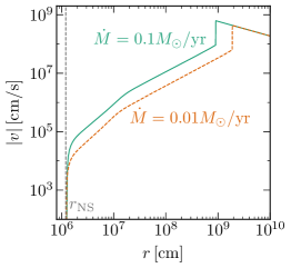
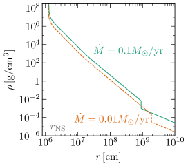
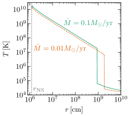
Figure A5: Velocity, density, and temperature profiles for Super-Eddington accretion flow onto a neutron star with a mass of $1.33\text{\,}\mathrm{M}_{\odot}$ and a radius of $12\text{\,}\mathrm{k}\mathrm{m}$. We show the results for accretion rates of $0.1\text{\,}\mathrm{M}_{\odot}\mathrm{/}\mathrm{y}\mathrm{r}$ and $0.01\text{\,}\mathrm{M}_{\odot}\mathrm{/}\mathrm{y}\mathrm{r}$, respectively.

B Neutrino emission

Below, we describe how we compute the neutrino flux given the temperature and density profiles. We follow Ref. Dicus:1972yr to compute the flux from electron–positron annihilation, and Ref. Braaten:1993jw to compute the flux from plasmon decay. We find that, due to the high temperature of the accretion flow, positron annihilation produces a much larger neutrino flux than plasmon decay. In this section, we use natural units ($\hbar=c=k_{B}=1$).

B.1 Positron annihilation

Thermally produced positrons can annihilate with electrons to produce $\nu\bar{\nu}$ pairs. The number of reactions per unit volume per unit time is Dicus:1972yr

$$R_{e^{+}e^{-}}=\int\!\frac{\mathop{\mathrm{\mathstrut d}}\nolimits^{3}\!{\vec{p}}_{\nu}}{(2\pi)^{3}2E_{\nu}}\frac{\mathop{\mathrm{\mathstrut d}}\nolimits^{3}\!{\vec{p}}_{\bar{\nu}}}{(2\pi)^{3}2E_{\bar{\nu}}}\frac{\mathop{\mathrm{\mathstrut d}}\nolimits^{3}\!{\vec{p}}_{e^{-}}}{(2\pi)^{3}2E_{e^{-}}}\frac{\mathop{\mathrm{\mathstrut d}}\nolimits^{3}\!{\vec{p}}_{e^{+}}}{(2\pi)^{3}2E_{e^{+}}}\,(2\pi)^{4}\delta^{4}(p_{e^{-}}+p_{e^{+}}-p_{\nu}-p_{\bar{\nu}})\,f_{e^{-}}(E_{e^{-}})\,f_{e^{+}}(E_{e^{+}})\,|\mathcal{M}|^{2}\,,$$ (B22)

with $p_{\nu}$, $p_{\bar{\nu}}$, $p_{e^{-}}$, and $p_{e^{+}}$ the four-momenta of the neutrino, antineutrino, electron, and positron, respectively; $\vec{p}_{\nu}$, $\vec{p}_{\bar{\nu}}$, $\vec{p}_{e^{-}}$, and $\vec{p}_{e^{+}}$ their three-momenta; $E_{\nu}$, $E_{\bar{\nu}}$, $E_{e^{-}}$, and $E_{e^{+}}$ their energies; $f_{e^{-}}$ and $f_{e^{+}}$ Fermi-Dirac distributions for electrons and positrons, respectively; and $|\mathcal{M}|^{2}$ the weak-interaction matrix element

$$|\mathcal{M}|^{2}=8G_{F}^{2}\left[(C_{V}-C_{A})^{2}(p_{e^{-}}\cdot p_{\nu})(p_{e^{+}}\cdot p_{\bar{\nu}})+(C_{V}+C_{A})^{2}(p_{e^{-}}\cdot p_{\bar{\nu}})(p_{e^{+}}\cdot p_{\nu})+m_{e}^{2}(C_{V}^{2}-C_{A}^{2})(p_{\nu}\cdot p_{\bar{\nu}})\right]\,.$$ (B23)

In this expression, $G_{F}$ is Fermi’s constant, $m_{e}$ the electron mass, and $C_{V}$ and $C_{A}$ the vector and axial couplings that depend on the neutrino flavor,

$$C_{V} =\frac{1}{2}+2\sin^{2}\theta_{W}\qquad\qquad \nu_{e}$$ for , (B24)

$$C_{V} =-\frac{1}{2}+2\sin^{2}\theta_{W} \nu_{\mu} \nu_{\tau}$$ for and , (B25)

$$C_{A} =\frac{1}{2} \nu_{e}$$ for , (B26)

$$C_{A} =-\frac{1}{2} \nu_{\mu} \nu_{\tau}$$ for and . (B27)

Here, $\theta_{W}$ is the weak mixing angle. Following Ref. Kato:2015faa , we write

$$\frac{\mathop{\mathrm{\mathstrut d}}\nolimits\!R_{e^{+}e^{-}}}{\mathop{\mathrm{\mathstrut d}}\nolimits\!E_{\nu}\mathop{\mathrm{\mathstrut d}}\nolimits\!E_{\bar{\nu}}\mathop{\mathrm{\mathstrut d}}\nolimits\!\cos\theta}=\frac{4E_{\nu}E_{\bar{\nu}}}{(2\pi)^{6}}G_{F}^{2}\left[\beta_{1}I_{1}+\beta_{2}I_{2}+\beta_{3}I_{3}\right]\,,$$ (B28)

where $\theta$ is the angle between the neutrino and antineutrino, the coefficients $\beta_{i}$ ($i\in\{1,2,3\}$) are defined as

$$\beta_{1} \equiv(C_{V}-C_{A})^{2}\,,$$ (B29)

$$\beta_{2} \equiv(C_{V}+C_{A})^{2}\,,$$ (B30)

$$\beta_{3} \equiv C_{V}^{2}-C_{A}^{2}\,;$$ (B31)

and the integrals $I_{i}$ ($i\in\{1,2,3\}$) are

$$I_{1} =\int\frac{\mathop{\mathrm{\mathstrut d}}\nolimits^{3}\!{\vec{p}}_{e^{-}}}{(2\pi)^{3}2E_{e^{-}}}\frac{\mathop{\mathrm{\mathstrut d}}\nolimits^{3}\!{\vec{p}}_{e^{+}}}{(2\pi)^{3}2E_{e^{+}}}\delta^{4}(p_{e^{-}}+p_{e^{+}}-p_{\nu}-p_{\bar{\nu}})\frac{f_{e^{-}}(E_{e^{-}})f_{e^{+}}(E_{e^{+}})}{4}(p_{e^{-}}\cdot p_{\nu})^{2}\,,$$ (B32)

$$I_{2} =\int\frac{\mathop{\mathrm{\mathstrut d}}\nolimits^{3}\!{\vec{p}}_{e^{-}}}{(2\pi)^{3}2E_{e^{-}}}\frac{\mathop{\mathrm{\mathstrut d}}\nolimits^{3}\!{\vec{p}}_{e^{+}}}{(2\pi)^{3}2E_{e^{+}}}\delta^{4}(p_{e^{-}}+p_{e^{+}}-p_{\nu}-p_{\bar{\nu}})\frac{f_{e^{-}}(E_{e^{-}})f_{e^{+}}(E_{e^{+}})}{4}(p_{e^{-}}\cdot p_{\bar{\nu}})^{2}\,,$$ (B33)

$$I_{3} =\int\frac{\mathop{\mathrm{\mathstrut d}}\nolimits^{3}\!{\vec{p}}_{e^{-}}}{(2\pi)^{3}2E_{e^{-}}}\frac{\mathop{\mathrm{\mathstrut d}}\nolimits^{3}\!{\vec{p}}_{e^{+}}}{(2\pi)^{3}2E_{e^{+}}}\delta^{4}(p_{e^{-}}+p_{e^{+}}-p_{\nu}-p_{\bar{\nu}})\frac{f_{e^{-}}(E_{e^{-}})f_{e^{+}}(E_{e^{+}})}{4}m_{e}^{2}(p_{\nu}\cdot p_{\bar{\nu}})\,.$$ (B34)

We integrate over $\vec{p}_{e^{+}}$ by writing

$$\int\frac{\mathop{\mathrm{\mathstrut d}}\nolimits^{3}\!{\vec{p}}_{e^{+}}}{E_{e^{+}}}=2\int\mathop{\mathrm{\mathstrut d}}\nolimits^{4}\!p_{e^{+}}\delta(p_{e^{+}}^{2}-m_{e}^{2})\Theta(E_{e^{+}})\,$$ (B35)

(with $\Theta$ the Heaviside step function), and then eliminating the integral using the $\delta^{(4)}$ functions in Eqs. B32, B33 and B34. To carry out the remaining integrals, we take $\vec{p}_{\nu}+\vec{p}_{\bar{\nu}}$ along the $z$-axis, and we obtain

$$\begin{split}I_{1}(E_{\nu},E_{\bar{\nu}},\cos\theta)=-\frac{2\pi TE_{\nu}^{2}E_{\bar{\nu}}^{2}(1-\cos\theta)^{2}}{\Delta_{e}^{5}\left[e^{(E_{\nu}+E_{\bar{\nu}})/T}-1\right]}\{&AT^{2}[y_{\mathrm{max}}^{2}G_{0}(y_{\mathrm{max}})-y_{\mathrm{min}}^{2}G_{0}(y_{\mathrm{min}})\\ &\phantom{AT^{2}[}+2y_{\mathrm{max}}G_{1}(y_{\mathrm{max}})-2y_{\mathrm{min}}G_{1}(y_{\mathrm{min}})\\ &\phantom{AT^{2}[}+G_{2}(y_{\mathrm{max}})-G_{2}(y_{\mathrm{min}})]\\ &+BT[y_{\mathrm{max}}G_{0}(y_{\mathrm{max}})-y_{\mathrm{min}}G_{0}(y_{\mathrm{min}})\\ &\phantom{+BT[}+G_{1}(y_{\mathrm{max}})-G_{1}(y_{\mathrm{min}})]\\ &+C[G_{0}(y_{\mathrm{max}})-G_{0}(y_{\mathrm{min}})]\}\,,\end{split}$$ (B36)

where $T$ is the temperature of the system,

$$\Delta_{e} \equiv\sqrt{E_{\nu}^{2}+E_{\bar{\nu}}^{2}+2E_{\nu}E_{\bar{\nu}}\cos\theta}\,,$$ (B37)

$$A \equiv E_{\bar{\nu}}^{2}+E_{\nu}^{2}-E_{\nu}E_{\bar{\nu}}(3+\cos\theta)\,,$$ (B38)

$$B \equiv E_{\nu}[-2E_{\nu}^{2}+E_{\bar{\nu}}^{2}(1+3\cos\theta)+E_{\nu}E_{\bar{\nu}}(3-\cos\theta)]\,,$$ (B39)

$$C \equiv E_{\nu}^{2}\left[(E_{\nu}+E_{\bar{\nu}}\cos\theta)^{2}-\frac{1}{2}E_{\bar{\nu}}^{2}(1-\cos^{2}\theta)-\frac{1}{2E_{\nu}^{2}}m_{e}^{2}\Delta_{e}^{2}\frac{1+\cos\theta}{1-\cos\theta}\right]\,,$$ (B40)

$$y^{\mathrm{max}}_{\mathrm{min}} \equiv\frac{E_{\nu}+E_{\bar{\nu}}\pm\Delta_{e}\sqrt{1-\frac{2m_{e}^{2}}{E_{\nu}E_{\bar{\nu}}(1-\cos\theta)}}}{2T}\,,$$ (B41)

$$G_{n}(y) \equiv F_{n}\left(\frac{E_{\nu}+E_{\bar{\nu}}+\mu}{T}-y\right)-F_{n}\left(\frac{\mu}{T}-y\right)\,,$$ (B42)

$$F_{n}(y) \equiv\int_{0}^{\infty}\frac{t^{n}}{e^{t-x}+1}\,\mathop{\mathrm{\mathstrut d}}\nolimits\!t\,,$$ (B43)

and $\mu$ is the electron chemical potential including electron mass. The other integrals are simpler,

$$I_{2}(E_{\nu},E_{\bar{\nu}},\cos\theta) =I_{1}(E_{\nu}=E_{\bar{\nu}},E_{\bar{\nu}}=E_{\nu},\cos\theta)\,,$$ (B44)

$$I_{3}(E_{\nu},E_{\bar{\nu}},\cos\theta) =-\frac{2\pi Tm_{e}^{2}E_{\nu}E_{\bar{\nu}}(1-\cos\theta)}{\Delta_{e}\left[e^{(E_{\nu}+E_{\bar{\nu}})/T}-1\right]}[G_{0}(y_{\mathrm{max}})-G_{0}(y_{\mathrm{min}})]\,.$$ (B45)

The number of neutrinos produced per unit volume, time, and energy is then

$$\frac{\mathop{\mathrm{\mathstrut d}}\nolimits\!R_{e^{+}e^{-}}}{\mathop{\mathrm{\mathstrut d}}\nolimits\!E_{\nu}}=\int\frac{\mathop{\mathrm{\mathstrut d}}\nolimits\!R_{e^{+}e^{-}}}{\mathop{\mathrm{\mathstrut d}}\nolimits\!E_{\nu}\mathop{\mathrm{\mathstrut d}}\nolimits\!E_{\bar{\nu}}\mathop{\mathrm{\mathstrut d}}\nolimits\!\cos\theta}\,\mathop{\mathrm{\mathstrut d}}\nolimits\!E_{\bar{\nu}}\,\mathop{\mathrm{\mathstrut d}}\nolimits\!\cos\theta\,,$$ (B46)

where $\cos\theta\in\left[-1,1-2m_{e}^{2}/(E_{\nu}E_{\bar{\nu}})\right]$. The antineutrino spectrum is identical to the neutrino spectrum.

Figure B6 shows the neutrino spectrum at a temperature of $1.5\text{\times}{10}^{10}\text{\,}\mathrm{K}$, characteristic of super-Eddington common-envelope events (see Figs. 2 and A5). At such high temperatures, electrons are mainly of thermal origin, so the spectrum is independent of density to a good approximation. As mentioned in the main text, the average neutrino energy is on the order of the average electron energy, and the neutrino spectrum is approximately thermal. We have checked that the energy loss rate, $\displaystyle\int(E_{\nu}+E_{\bar{\nu}})\frac{\mathop{\mathrm{\mathstrut d}}\nolimits\!R_{e^{+}e^{-}}}{\mathop{\mathrm{\mathstrut d}}\nolimits\!E_{\nu}\mathop{\mathrm{\mathstrut d}}\nolimits\!E_{\bar{\nu}}\mathop{\mathrm{\mathstrut d}}\nolimits\!\cos\theta}\mathop{\mathrm{\mathstrut d}}\nolimits\!E_{\nu}\,\mathop{\mathrm{\mathstrut d}}\nolimits\!E_{\bar{\nu}}\,\mathop{\mathrm{\mathstrut d}}\nolimits\!\cos\theta$, reproduces the results in Refs. Dicus:1972yr ; Itoh:1996 .

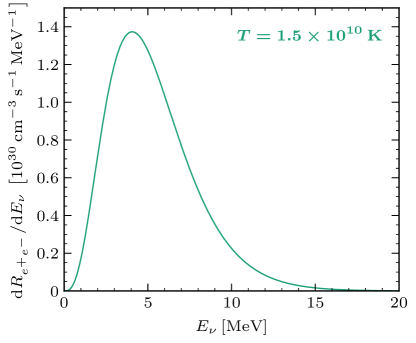
Figure B6: All-flavor neutrino spectrum due to thermal positron annihilation, at temperatures typical in a super-Eddington common-envelope event. The antineutrino spectrum is identical.

B.2 Plasmon decay

We compute the subdominant neutrino flux from plasmon decays closely following Ref. Braaten:1993jw . The neutrino emission rate per unit volume per unit energy receives contributions from transverse and longitudinal plasmon decay,

$$\frac{\mathop{\mathrm{\mathstrut d}}\nolimits\!R_{\gamma^{*}}}{\mathop{\mathrm{\mathstrut d}}\nolimits\!E_{\nu}} =\int\!\frac{4\pi k^{2}\mathop{\mathrm{\mathstrut d}}\nolimits\!k}{(2\pi)^{3}}\,\Big{[}2\,n_{B}[\omega_{t}(k)]\,\frac{\mathop{\mathrm{\mathstrut d}}\nolimits\!\Gamma_{t}(k)}{\mathop{\mathrm{\mathstrut d}}\nolimits\!E_{\nu}}+n_{B}[\omega_{l}(k)]\,\frac{\mathop{\mathrm{\mathstrut d}}\nolimits\!\Gamma_{l}(k)}{\mathop{\mathrm{\mathstrut d}}\nolimits\!E_{\nu}}\Big{]}\,,$$ (B47)

where the integral runs over plasmon momenta $k$,

$$n_{B}(\omega)=\frac{1}{e^{\omega/T}-1}$$ (B48)

is the Bose–Einstein distribution describing the plasmon population, and $\omega_{t}(k)$ and $\omega_{l}(k)$ are the frequencies of transverse and longitudinal plasmons, respectively. The latter quantities are the solutions of the dispersion relations, which in the Coulomb gauge read

$$[\omega_{t}(k)]^{2}-k^{2}-\Pi_{t}^{(e)}[\omega_{t}(k),k]-\Pi_{t}^{(p)}[\omega_{t}(k),k] =0\,,$$ (B49)

$$[k^{2}-\Pi_{l}^{(e)}[\omega_{t}(k),k]-\Pi_{l}^{(p)}[\omega_{t}(k),k] =0\,.$$ (B50)

They contain the polarization functions (self-energies)

$$\Pi_{t}^{(f)}(\omega,k) =\frac{4\alpha}{\pi}\int_{0}^{\infty}\!\mathop{\mathrm{\mathstrut d}}\nolimits\!p\,\frac{p^{2}}{E_{f}}\bigg{(}\frac{\omega^{2}}{k^{2}}-\frac{\omega^{2}-k^{2}}{k^{2}}\frac{\omega}{2v_{f}k}\log\frac{\omega+v_{f}k}{\omega-v_{f}k}\bigg{)}\big{[}n_{F}(E_{f})+\bar{n}_{F}(E_{f})\big{]}\,,$$ (B51)

$$\Pi_{l}^{(f)}(\omega,k) =\frac{4\alpha}{\pi}\int_{0}^{\infty}\!\mathop{\mathrm{\mathstrut d}}\nolimits\!p\,\frac{p^{2}}{E_{f}}\bigg{(}\frac{\omega}{v_{f}k}\log\frac{\omega+v_{f}k}{\omega-v_{f}k}-1-\frac{\omega^{2}-k^{2}}{\omega^{2}-v_{f}^{2}k^{2}}\bigg{)}\big{[}n_{F}(E_{f})+\bar{n}_{F}(E_{f})\big{]}\,.$$ (B52)

In these expressions, the integrals run over fermion (electron or proton) momenta, $p$; $E_{f}=(p^{2}+m_{f}^{2})^{1/2}$ is the corresponding fermion energy; $v_{f}=p/E_{f}$ is the velocity; and

$$n_{F}(E_{f}) =\frac{1}{e^{(E_{f}-\mu_{f})/T}+1}\,,$$ (B53)

$$\bar{n}_{F}(E_{f}) =\frac{1}{e^{(E_{f}+\mu_{f})/T}+1}$$ (B54)

are, respectively, the fermion and anti-fermion thermal (Fermi–Dirac) distributions at temperature $T$ and chemical potential $\mu_{f}$. The differential plasmon decay rates are given by

$$\frac{\mathop{\mathrm{\mathstrut d}}\nolimits\!\Gamma_{t}(k)}{\mathop{\mathrm{\mathstrut d}}\nolimits\!E_{\nu}} =\frac{G_{F}^{2}}{16\pi^{2}\alpha}Z_{t}(k)\frac{\omega_{t}(k)^{2}-k^{2}}{\omega_{t}(k)}\Big{[}\Big{(}C_{V}\Pi_{t}^{(e)}[\omega_{t}(k),k]-h_{V}\Pi_{t}^{(p)}[\omega_{t}(k),k]\Big{)}^{2}$$

$$\hskip 110.96556pt+\Big{(}C_{A}\Pi_{A}^{(e)}[\omega_{t}(k),k]-h_{A}\Pi_{A}^{(p)}[\omega_{t}(k),k]\Big{)}^{2}\Big{]}\frac{k^{2}+(\omega_{t}(k)-2E_{\nu})^{2}}{4k^{3}}$$

$$\hskip 56.9055pt+\Big{(}C_{V}\Pi_{t}^{(e)}[\omega_{t}(k),k]-h_{V}\Pi_{t}^{(p)}[\omega_{t}(k),k]\Big{)}\Big{(}C_{A}\Pi_{A}^{(e)}[\omega_{t}(k),k]-h_{A}\Pi_{A}^{(p)}[\omega_{t}(k),k]\Big{)}\frac{\omega_{t}(k)-2E_{\nu}}{k^{2}}\,,$$ (B55)

$$\frac{\mathop{\mathrm{\mathstrut d}}\nolimits\!\Gamma_{l}(k)}{\mathop{\mathrm{\mathstrut d}}\nolimits\!E_{\nu}} =\frac{G_{F}^{2}}{32\pi^{2}\alpha}Z_{l}(k)\big{(}[\omega_{l}(k)]^{2}-k^{2}\big{)}^{2}\,\frac{\omega_{l}(k)}{k^{5}}\Big{(}C_{V}\Pi_{l}^{(e)}[\omega_{l}(k),k]-h_{V}\Pi_{l}^{(p)}[\omega_{l}(k),k]\Big{)}^{2}\,\left[1-\left(\frac{\omega_{l}(k)-2E_{\nu}}{k}\right)^{2}\right]\,.$$ (B56)

They depend on the vector and axial-vector couplings, $C_{V}$ and $C_{A}$, between neutrinos and the electrons in the plasma (given by Eqs. B24, B25, B26 and B27), and on the corresponding couplings to protons, $h_{V}$ and $h_{A}$,

$$h_{V} =\frac{1}{2}-2\sin^{2}\theta_{W}\,,$$ (B57)

$$h_{A} =\frac{1}{2}g_{A}\,,$$ (B58)

with the axial coupling constant $g_{A}\simeq 1.26$. Unlike for $C_{V}$ and $C_{A}$, the couplings to protons are the same for all neutrino flavors. The axial polarization function $\Pi_{A}(\omega,k)^{(f)}$ appearing in Eq. B55 is

$$\Pi_{A}^{(f)}(\omega,k) =\frac{2\alpha}{\pi}\frac{\omega^{2}-k^{2}}{k}\int_{0}^{\infty}\!\mathop{\mathrm{\mathstrut d}}\nolimits\!p\,\frac{p^{2}}{E_{f}^{2}}\bigg{(}\frac{\omega}{2v_{f}k}\log\frac{\omega+v_{f}k}{\omega-v_{f}k}-\frac{\omega^{2}-k^{2}}{\omega^{2}-v_{f}^{2}k^{2}}\bigg{)}\big{[}n_{F}(E_{f})-\bar{n}_{F}(E_{f})\big{]}\,,$$ (B59)

and the quantities $Z_{t}(k)$ and $Z_{l}(k)$ are the residues of the plasmon propagators at the pole, which can be interpreted as in-medium corrections to the plasmon field strengths. They are given by

$$Z_{t}(k) \equiv\bigg{[}1-\frac{\partial\Pi_{t}[\omega,k]}{\partial\omega^{2}}\Big{|}_{\omega=\omega_{t}(k)}\bigg{]}^{-1}\,,$$ (B60)

$$Z_{l}(k) \equiv\frac{k^{2}}{\omega_{l}(k)^{2}}\bigg{[}-\frac{\partial\Pi_{l}[\omega,k]}{\partial\omega^{2}}\Big{|}_{\omega=\omega_{l}(k)}\bigg{]}^{-1}\,.$$ (B61)

Here, $\Pi_{t}\equiv\Pi_{t}^{(e)}+\Pi_{t}^{(p)}$ and similarly for $\Pi_{l}\equiv\Pi_{l}^{(e)}+\Pi_{l}^{(p)}$.

It is in principle feasible to numerically compute the integrals appearing in Eqs. B47, B51, B52 and B59, as well as the solutions to the dispersion relations Eqs. B49 and B50. In practice, however, it is much more efficient to use the very accurate analytical approximations derived in Ref. Braaten:1993jw . Notably, the polarization functions from Eqs. B51, B52 and B59 can be approximated as

$$\Pi_{t}(\omega,k) \simeq\omega_{p}^{2}\,\frac{3}{2v_{*}^{2}}\bigg{(}\frac{\omega^{2}}{k^{2}}-\frac{\omega^{2}-v_{*}^{2}k^{2}}{k^{2}}\frac{\omega}{2v_{*}k}\log\frac{\omega+v_{*}k}{\omega-v_{*}k}\bigg{)}\,,$$ (B62)

$$\Pi_{l}(\omega,k) \simeq\omega_{p}^{2}\frac{3}{v_{*}^{2}}\bigg{(}\frac{\omega}{2v_{*}k}\log\frac{\omega+v_{*}k}{\omega-v_{*}k}-1\bigg{)}\,,$$ (B63)

$$\Pi_{A}(\omega,k) \simeq\omega_{A}\frac{\omega^{2}-k^{2}}{k}\frac{3}{v_{*}^{2}}\bigg{(}\frac{\omega}{2v_{*}k}\log\frac{\omega+v_{*}k}{\omega-v_{*}k}-1\bigg{)}\,,$$ (B64)

with the definitions

$$v_{*} \equiv\frac{\omega_{1}}{\omega_{p}}\,,$$ (B65)

$$\omega_{p}^{2} \equiv\frac{4\alpha}{\pi}\int_{0}^{\infty}\!\mathop{\mathrm{\mathstrut d}}\nolimits\!p\,\frac{p^{2}}{E}\Big{(}1-\tfrac{1}{3}v^{2}\Big{)}\big{[}n_{F}(E)+\bar{n}_{F}(E)\big{]}\,,$$ (B66)

$$\omega_{1}^{2} \equiv\frac{4\alpha}{\pi}\int_{0}^{\infty}\!\mathop{\mathrm{\mathstrut d}}\nolimits\!p\,\frac{p^{2}}{E}\Big{(}\tfrac{5}{3}v^{2}-v^{4}\Big{)}\big{[}n_{F}(E)+\bar{n}_{F}(E)\big{]}\,,$$ (B67)

$$\omega_{A}^{2} \equiv\frac{2\alpha}{\pi}\int_{0}^{\infty}\!\mathop{\mathrm{\mathstrut d}}\nolimits\!p\,\frac{p^{2}}{E^{2}}\Big{(}1-\tfrac{2}{3}v^{2}\Big{)}\big{[}n_{F}(E)-\bar{n}_{F}(E)\big{]}\,.$$ (B68)

$\omega_{p}$ is the plasma frequency, and $\omega_{1}$ is a measure for the first relativistic correction to it. Here, we have omitted superscripts indicating the fermion species ($f=e,p$) to shorten the notation. Plugging Eqs. B62 and B63 into Eqs. B60 and B61 yields approximate expressions also for $Z_{t}(k)$ and $Z_{l}(k)$. We have checked the excellent agreement between the analytic approximations and the full numerical result in the parameter region relevant for us.

Figure B7: All-flavor neutrino spectrum due to plasmon decay, at temperatures and densities typical in a super-Eddington common-envelope event. The antineutrino spectrum is identical. Note the very large vertical scale change compared to Fig. B6.

Figure B7 shows the neutrino spectrum from plasmon decay at a temperature of $1.5\text{\times}{10}^{10}\text{\,}\mathrm{K}$ and a density of ${10}^{7}\text{\,}\mathrm{g}\mathrm{/}\mathrm{c}\mathrm{m}^{3}$, characteristic of super-Eddington common-envelope events (see Figs. 2 and A5). At such high temperatures, electron densities entering Eqs. B51, B52 and B59 are mainly of thermal origin, so the spectrum is not very dependent on density. As mentioned in the main text, at the high temperatures relevant for us the main production channel is positron annihilation, since plasmon decay is suppressed by $\alpha^{2}$. The average neutrino energy is smaller than the average plasmon energy because each plasmon decay produces a neutrino and an antineutrino. We have checked that the energy loss rate,

$$\int\!\frac{4\pi k^{2}\mathop{\mathrm{\mathstrut d}}\nolimits\!k}{(2\pi)^{3}}\,\Big{[}2\omega_{t}(k)\,n_{B}[\omega_{t}(k)]\,\frac{\mathop{\mathrm{\mathstrut d}}\nolimits\!\Gamma_{t}(k)}{\mathop{\mathrm{\mathstrut d}}\nolimits\!E_{\nu}}+\omega_{l}(k)\,n_{B}[\omega_{l}(k)]\,\frac{\mathop{\mathrm{\mathstrut d}}\nolimits\!\Gamma_{l}(k)}{\mathop{\mathrm{\mathstrut d}}\nolimits\!E_{\nu}}\Big{]}\,,$$ (B69)

reproduces the results in Refs. Braaten:1993jw ; Itoh:1996 .

B.3 Putting everything together

The results in this section, together with the temperature and density profiles computed in Section A, allow us to predict the neutrino flux from a super-Eddington common-envelope event. We conservatively assume the neutron star to be completely opaque to neutrinos Fattoyev:2017ybi . Since neutrino emission is isotropic, this suppresses the flux emitted from a radius $r$ by a factor

$$\frac{1}{2}+\sqrt{1-\left(\frac{r_{\mathrm{NS}}}{r}\right)^{2}}\,,$$ (B70)

an effect that reduces the neutrino flux by about 30%. In addition, neutrinos emitted very close to the neutron star undergo gravitational redshift. Their energy measured far away, $E_{\nu}$, is related to the energy at production, $E_{\nu}^{\mathrm{prod}}$, by

$$E_{\nu}=E_{\nu}^{\mathrm{prod}}\sqrt{1-\frac{2GM_{\mathrm{NS}}}{r}}\equiv E_{\nu}^{\mathrm{prod}}\sqrt{1-\frac{r_{s}}{r}}\,,$$ (B71)

with $r$ the radius where the neutrino is produced and $r_{s}$ the Schwarzschild radius. This effect reduces neutrino energies by about 20%.

Putting everything together, the neutrino flux measured at Earth is

$$\frac{\mathop{\mathrm{\mathstrut d}}\nolimits\!\phi_{\nu}}{\mathop{\mathrm{\mathstrut d}}\nolimits\!E_{\nu}}=\frac{1}{4\pi d^{2}}\int\mathop{\mathrm{\mathstrut d}}\nolimits\!r\mathop{\mathrm{\mathstrut d}}\nolimits\!t\,4\pi r^{2}\,\left[\frac{1}{2}+\sqrt{1-(r_{\mathrm{NS}}/r)^{2}}\right]\,\frac{\mathop{\mathrm{\mathstrut d}}\nolimits\!R}{\mathop{\mathrm{\mathstrut d}}\nolimits\!E_{\nu}}\left(\frac{E_{\nu}}{\sqrt{1-r_{s}/r}},\,\rho(r,\dot{M}(t)),\,T(r,\dot{M}(t))\right)\,,$$ (B72)

with $d$ the distance to the source and $\mathop{\mathrm{\mathstrut d}}\nolimits\!R/\mathop{\mathrm{\mathstrut d}}\nolimits\!E_{\nu}\equiv\mathop{\mathrm{\mathstrut d}}\nolimits\!R_{e^{+}e^{-}}/\mathop{\mathrm{\mathstrut d}}\nolimits\!E_{\nu}+\mathop{\mathrm{\mathstrut d}}\nolimits\!R_{\gamma^{*}}/\mathop{\mathrm{\mathstrut d}}\nolimits\!E_{\nu}$. $\rho$ and $T$ depend on the accretion rate $\dot{M}$, as it enters the equations of hydrodynamics via Eq. A4.

Figure C8 shows the amount of neutrinos per unit energy produced in the last 3 months of the common-envelope simulation of Ref. MacLeod:2014yda . As described in the main text, most neutrinos are emitted as $\nu_{e}$ and $\bar{\nu}_{e}$. The average neutrino energy and flux are very similar to the order-of-magnitude estimates in the main text ($\sim$4\text{\,}\mathrm{M}\mathrm{e}\mathrm{V}$$ and $\sim${10}^{50}\text{\,}\mathrm{n}\mathrm{e}\mathrm{u}\mathrm{t}\mathrm{r}\mathrm{i}\mathrm{n}\mathrm{o}\mathrm{s}\mathrm{/}\mathrm{s}$=${10}^{57}\text{\,}\mathrm{n}\mathrm{e}\mathrm{u}\mathrm{t}\mathrm{r}\mathrm{i}\mathrm{n}\mathrm{o}\mathrm{s}\mathrm{/}\mathrm{(}\mathrm{3}\,\mathrm{m}\mathrm{o}\mathrm{n}\mathrm{t}\mathrm{h}\mathrm{s}\mathrm{)}$$, respectively), which follow from energy-conservation arguments. For comparison, the total amount of neutrinos is about 10% of the number of neutrinos emitted in a core-collapse supernova, albeit for neutrinos from common-envelope evolution energies are smaller and the emission time is longer.

C Neutrino oscillations

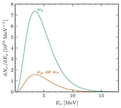
Figure C8: Neutrino spectrum from common-envelope super-Eddington accretion, using the simulation from Ref. MacLeod:2014yda and integrating over 3 months. Neutrino oscillations are not included. The antineutrino spectrum is identical.

For completeness, we briefly mention here our treatment of neutrino oscillations (for a more complete overview of oscillations in a dense environment, see Ref. Dighe:1999bi ). We include adiabatic transitions, as non-adiabatic corrections only modify our results by $\lesssim 10\%$ Kuo:1989qe ; Maltoni:2015kca ; and we use the mixing parameters from Ref. Esteban:2020cvm . Overall, oscillations change the common-envelope signal by a factor of few.

Thermal neutrino emission produces the same amount of $\nu_{\mu}$ and $\nu_{\tau}$. Furthermore, at the energies we consider it is very challenging to experimentally distinguish between them Brdar:2023ttb . Hence, we can consider an effective 2-flavor problem, and write the $\nu_{e}$ flux at Earth as

$$\phi_{e}=\phi_{e}^{0}P_{ee}+\phi_{x}^{0}(1-P_{ee})\,,$$ (C73)

where $\phi_{e}^{0}$ and $\phi_{x}^{0}$ are the initial fluxes of $\nu_{e}$ and $\nu_{\mu}$ (or $\nu_{\tau}$), respectively; and $P_{ee}$ is the $\nu_{e}\rightarrow\nu_{e}$ transition probability. The average of the $\nu_{\mu}$ and $\nu_{\tau}$ fluxes at Earth is given by

$$\phi_{x}\equiv\frac{\phi_{\mu}+\phi_{\tau}}{2}=\frac{1}{2}\left[\phi_{e}^{0}(1-P_{ee})+\phi_{x}^{0}(1+P_{ee})\right]\,.$$ (C74)

Analogously, for antineutrinos

$$\phi_{\bar{e}} =\phi_{\bar{e}}^{0}P_{\bar{e}\bar{e}}+\phi_{\bar{x}}^{0}(1-P_{\bar{e}\bar{e}})\,,$$ (C75)

$$\phi_{\bar{x}}\equiv\frac{\phi_{\bar{\mu}}+\phi_{\bar{\tau}}}{2} =\frac{1}{2}\left[\phi_{e}^{0}(1-P_{\bar{e}\bar{e}})+\phi_{x}^{0}(1+P_{\bar{e}\bar{e}})\right]\,,$$ (C76)

where bars indicate the corresponding antineutrino flux and $P_{\bar{e}\bar{e}}$ is the $\bar{\nu}_{e}\rightarrow\bar{\nu}_{e}$ transition probability.

In a dense environment, transitions happen mainly when the density equals the resonant density, $\sim 10^{3}$–$\qty{e4}{g/cm^{3}}$ for the atmospheric mass splitting and $\sim 10$–$30\text{\,}\mathrm{g}\mathrm{/}\mathrm{c}\mathrm{m}^{3}$ for the solar mass splitting. Neutrinos from a super-Eddington common-envelope event cross both resonance regions (see Fig. A5), but which resonances they actually experience depends on the neutrino mass ordering.

In the normal mass ordering (NO), an initial $\nu_{e}$ experiences both resonances, exiting the star as a $\nu_{3}$ mass eigenstate, and $P_{ee}=|U_{e3}|^{2}\simeq 0.022$. In the inverted mass ordering (IO), only the solar resonance lies in the neutrino sector, and $P_{ee}=|U_{e2}|^{2}\simeq 0.30$. For antineutrinos, the picture is different: in the NO, all resonances lie in the neutrino sector, and $P_{\bar{e}\bar{e}}=|U_{e1}|^{2}\simeq 0.68$; and in the IO the atmospheric resonance lies in the antineutrino sector, and $P_{\bar{e}\bar{e}}=|U_{e3}|^{2}\simeq 0.022$. This is why for the IO the signal in Super-K and JUNO, which rely on inverse beta decay, is suppressed in Fig. 3. The remaining events in these experiments are then mostly due to $\bar{\nu}_{\mu}$ and $\bar{\nu}_{\tau}$ converting into $\bar{\nu}_{e}$. Since the number of initially produced $\bar{\nu}_{\mu}$ and $\bar{\nu}_{\tau}$ is smaller than the number of initially produced $\bar{\nu}_{e}$, the overall signal is suppressed. Neutrino–electron scattering in DUNE has some sensitivity to all neutrino flavors, so the expected rates are more similar for both mass orderings.

D Details of experiment simulations

Here, we provide details on how we simulate the various experiments considered in Figs. 3 and 4 in the main text. We aim to be conservative in our assumptions, leaving a lot of room for improvement by dedicated searches carried out within the experimental collaborations.

In each case we consider, the neutrino energy is estimated by reconstructing the energy of the electron or positron produced when the neutrino interacts. The number of events with reconstructed electron/positron energy $\in[E_{e}^{\mathrm{min}},E_{e}^{\mathrm{max}}]$ from a common-envelope system is given by

$$N_{\mathrm{evt}}=\int_{E_{e}^{\mathrm{min}}}^{E_{e}^{\mathrm{max}}}\mathop{\mathrm{\mathstrut d}}\nolimits\!E_{e}^{\mathrm{rec}}\int_{0}^{\infty}\mathop{\mathrm{\mathstrut d}}\nolimits\!E_{e}\int_{0}^{\infty}\mathop{\mathrm{\mathstrut d}}\nolimits\!E_{\nu}\,\frac{\mathop{\mathrm{\mathstrut d}}\nolimits\!\phi_{\nu}(E_{\nu})}{\mathop{\mathrm{\mathstrut d}}\nolimits\!E_{\nu}}\,\frac{\mathop{\mathrm{\mathstrut d}}\nolimits\!\sigma(E_{\nu},E_{e})}{\mathop{\mathrm{\mathstrut d}}\nolimits\!E_{e}}\,N_{\mathrm{targets}}\,f_{\mathrm{rec}}(E_{e}^{\mathrm{rec}},E_{e})\,\epsilon(E_{e})\,,$$ (D77)

with $E_{e}^{\mathrm{rec}}$ the reconstructed electron/positron energy, $E_{e}$ the true electron/positron energy, $E_{\nu}$ the neutrino energy, $\mathop{\mathrm{\mathstrut d}}\nolimits\!\sigma/\mathop{\mathrm{\mathstrut d}}\nolimits\!E_{e}$ the differential neutrino interaction cross section, $N_{\mathrm{targets}}$ the number of targets in the detector, $f_{\mathrm{rec}}(E_{e}^{\mathrm{rec}},E_{e})$ the energy response function (i.e., the differential probability for an electron/positron with true energy $E_{e}$ to be reconstructed with energy $E_{e}^{\mathrm{rec}}$), and $\epsilon$ the detection efficiency.

We compute the statistical significance of the signal against a background-only hypothesis with a Poissonian likelihood ratio,

$$\Delta\chi^{2}=2\sum_{\mathrm{bins}}\bigg{(}N_{\mathrm{bkg}}-N_{\mathrm{total}}+N_{\mathrm{total}}\log\frac{N_{\mathrm{total}}}{N_{\mathrm{bkg}}}\bigg{)}\,,$$ (D78)

with $N_{\mathrm{bkg}}$ the number of background events in a given bin, and $N_{\mathrm{total}}\equiv N_{\mathrm{evt}}+N_{\mathrm{bkg}}$. For Fig. 3, we use $2\text{\,}\mathrm{M}\mathrm{e}\mathrm{V}$-wide energy bins. For Fig. 4, we specify the bin widths below.

Below, we detail the parameters for each experiment and we describe the backgrounds.

D.1 Super-K (archival)

Our simulation for archival Super-Kamiokande data closely follows Ref. Super-Kamiokande:2021jaq , which looked for inverse beta decay events due to diffuse supernova background neutrino interactions by searching for positrons together with delayed $\gamma$ rays due to neutron capture on protons.

We take the inverse beta decay cross section at order $E_{\nu}/m_{N}$, with $m_{N}$ the nucleon mass, from Refs. Vogel:1999zy ; Strumia:2003zx . The fiducial volume contains $22.5\text{\,}\mathrm{k}\mathrm{t}\mathrm{o}\mathrm{n}\mathrm{n}\mathrm{e}$ of water, corresponding to $N_{\mathrm{targets}}\simeq 1.5\times 10^{33}$ free protons. For energy reconstruction, we assume Gaussian smearing with the Super-Kamiokande low-energy resolution Super-Kamiokande:2016yck

$$\sigma(E_{e})/\mathrm{MeV}=-0.0839+0.349\sqrt{E_{e}/\mathrm{MeV}}+0.0397E_{e}/\mathrm{MeV}\,.$$ (D79)

We extract the detection efficiency, rising from $\sim 5\%$ at $8\text{\,}\mathrm{M}\mathrm{e}\mathrm{V}$ to $\sim 20\%$ at $20\text{\,}\mathrm{M}\mathrm{e}\mathrm{V}$, from Fig. 18 in Ref. Super-Kamiokande:2021jaq . At the energies we consider, backgrounds are mainly due to accidental coincidences, ⁹Li produced via spallation and undergoing beta decay together with neutron emission (which leaves the same signature as inverse beta decay), neutral current interactions of atmospheric neutrinos (which induce nuclear $\gamma$-ray emission), and a small component from reactor antineutrino and charged current atmospheric neutrino interactions. We extract the backgrounds from Fig. 24 in Ref. Super-Kamiokande:2021jaq , rescaling them to the 3-month exposure we consider. We consider positron kinetic energies $E^{\mathrm{kin}}_{e}\equiv E_{e}-m_{e}c^{2}$ above $7.5\text{\,}\mathrm{M}\mathrm{e}\mathrm{V}$, and 2-MeV bins Super-Kamiokande:2021jaq .

D.2 Super-K (low Gd)

Our simulation for the first Super-Kamiokande run with gadolinium loading Beacom:2003nk (corresponding to 0.01% mass concentration of gadolinium) closely follows Ref. Super-Kamiokande:2023xup . The cross section and energy reconstruction are the same as for Super-K (archival). We extract the detection efficiency, rising from $\sim 15\%$ at $8\text{\,}\mathrm{M}\mathrm{e}\mathrm{V}$ to $\sim 25\%$ at $20\text{\,}\mathrm{M}\mathrm{e}\mathrm{V}$, from Fig. 1 in Ref. Super-Kamiokande:2023xup . The main background sources are the same as for Super-K (archival). Since some bins in Ref. Super-Kamiokande:2023xup are wider than $2\text{\,}\mathrm{M}\mathrm{e}\mathrm{V}$, we also simulate the backgrounds, finding good agreement with Ref. Super-Kamiokande:2023xup . In particular, we neglect the subleading accidental coincidence contribution Super-Kamiokande:2023xup , we compute theoretically the ⁹Li decay spectrum and rescale it to the normalization in Fig. 2 in Ref. Super-Kamiokande:2023xup (rescaling also to the 3-month exposure we consider), we extract the atmospheric contribution from Fig. 2 in Ref. Super-Kamiokande:2023xup (rescaling to the 3-month exposure we consider), and we simulate the reactor background using the publicly available SKReact code. We consider positron kinetic energies above $7.5\text{\,}\mathrm{M}\mathrm{e}\mathrm{V}$, and 2-MeV bins Super-Kamiokande:2023xup .

D.3 Super-K (Gd, optim.)

For an optimistic future upgrade of Super-Kamiokande, we assume a gadolinium concentration large enough to increase the detection efficiency for inverse beta decay events to $75\%$. This efficiency corresponds to the limit in which all neutrons are captured on gadolinium Super-Kamiokande:2023xup . We further assume that background levels can be kept as in Super-K (Gd), with reactor backgrounds increased proportionally to the detection efficiency increase. We take the same cross section and energy resolution as in Super-K (archival). We consider positron kinetic energies above $3.5\text{\,}\mathrm{M}\mathrm{e}\mathrm{V}$ (at the sensitivity limit shown in Fig. 4, backgrounds overwhelm the signal below $\sim$7\text{\,}\mathrm{M}\mathrm{e}\mathrm{V}$$), and 0.5-MeV bins.

D.4 JUNO

Our JUNO simulation closely follows Refs. JUNO:2021vlw ; JUNO:2023vyz . The cross section is the same as for Super-K (archival). The detector contains $1.44\times 10^{33}$ free protons JUNO:2015zny . For the energy resolution, we assume Gaussian smearing with JUNO:2021vlw

$$\sigma(E_{\mathrm{vis}})=E_{\mathrm{vis}}\sqrt{a^{2}/E_{\mathrm{vis}}+b^{2}+c^{2}/E_{\mathrm{vis}}^{2}}\,,$$ (D80)

where $E_{\mathrm{vis}}=E_{e}+m_{e}c^{2}$ the deposited energy after positron annihilation, $a=$0.0261\text{\,}\sqrt{MeV}$$, $b=0.0082$, and $c=$0.0123\text{\,}\mathrm{M}\mathrm{e}\mathrm{V}$$. We assume 73% detection efficiency JUNO:2021vlw . At the energies we consider, backgrounds are mainly due to reactor neutrinos, ⁹Li and ⁸He produced via spallation (which can undergo beta decay together with neutron emission), and neutral current interactions of atmospheric neutrinos. We extract the background from Fig. 9 in Ref. JUNO:2021vlw and Fig. 6 in Ref. JUNO:2023vyz , rescaling it to the 3-month exposure we consider. We consider $E_{\mathrm{vis}}>$5\text{\,}\mathrm{M}\mathrm{e}\mathrm{V}$$ (at the sensitivity limit shown in Fig. 4, backgrounds overwhelm the signal below $\sim$7.5\text{\,}\mathrm{M}\mathrm{e}\mathrm{V}$$), and 0.5-MeV bins.

D.5 Hyper-K

To simulate the Hyper-Kamiokande detector, we rescale signals and backgrounds from Super-K (archival) by a factor 187/22.5, reflecting the increase in fiducial volume of the 1-tank design. We conservatively assume the same energy resolution as in Super-K Hyper-Kamiokande:2018ofw . We also increase ⁹Li spallation backgrounds by a factor of 2.7 due to the detector’s shallower depth Hyper-Kamiokande:2018ofw . We consider positron kinetic energies above $7.5\text{\,}\mathrm{M}\mathrm{e}\mathrm{V}$, and 2-MeV bins Super-Kamiokande:2021jaq .

D.6 Hyper-K (Gd)

To simulate the Hyper-Kamiokande detector with gadolinium loading, we rescale signals and backgrounds from Super-K (Gd, optim.) by a factor 187/22.5, reflecting the increase in fiducial volume of the 1-tank design. We conservatively assume the same energy resolution as in Super-K Hyper-Kamiokande:2018ofw . We also increase ⁹Li spallation backgrounds by a factor of 2.7 due to the detector’s shallower depth Hyper-Kamiokande:2018ofw . We consider positron kinetic energies above $3.5\text{\,}\mathrm{M}\mathrm{e}\mathrm{V}$ (at the sensitivity limit shown in Fig. 4, backgrounds overwhelm the signal below $\sim$8\text{\,}\mathrm{M}\mathrm{e}\mathrm{V}$$), and 0.5-MeV bins.

D.7 DUNE

For our DUNE simulation, we closely follow Refs. Capozzi:2018dat ; Zhu:2018rwc ; DUNE:2020ypp , which analyzed the potential of the experiment to detect solar neutrinos.

We take the neutrino–electron scattering cross section for the different neutrino flavors from Ref. Formaggio:2012cpf . We assume a $40\text{\,}\mathrm{k}\mathrm{t}\mathrm{o}\mathrm{n}\mathrm{n}\mathrm{e}$ fiducial volume, corresponding to the four-module design. This corresponds to $N_{\mathrm{targets}}\simeq 1.1\times 10^{34}$ electrons. We assume Gaussian smearing with 7% energy resolution Castiglioni:2020tsu in electron kinetic energy. We extract the detection efficiency from Fig. 7.17 in Ref. DUNE:2020ypp . At the energies we consider, backgrounds are mainly due to neutrons from the surrounding rock and spallation products. We take them from Ref. Capozzi:2018dat , rescale them to the 3-month exposure we consider, and reduce them by considering a forward cone of half-angle $40^{\circ}$ Capozzi:2018dat . We consider electron kinetic energies above $5\text{\,}\mathrm{M}\mathrm{e}\mathrm{V}$ (at the sensitivity limit shown in Fig. 4, backgrounds overwhelm the signal below $\sim$7.5\text{\,}\mathrm{M}\mathrm{e}\mathrm{V}$$), and 0.5-MeV bins.

As discussed in the main text, in Fig. 3 we assume that solar neutrino interactions on ⁴⁰Ar can be efficiently removed by identifying final-state $\gamma$ rays from nuclear deexcitation. In Fig. 4 in the main text, we also show the distance reach if $\gamma$ rays can not be identified. In that case, there are additional backgrounds from interactions of solar and common-envelope neutrinos with ⁴⁰Ar. We include them by taking the interaction cross section from the public code SNoWGLoBES, and reduce them by considering a forward cone of half-angle $40^{\circ}$ Capozzi:2018dat .

E Distance reach for the inverted mass ordering

In Fig. 4 in the main text, we show the distance reach to super-Eddington neutron-star common-envelope events assuming the normal mass ordering, which is currently favored over the inverted mass ordering by $\sim 2.5\sigma$ Esteban:2020cvm . Figure E9 shows the distance reach for the inverted ordering. As described in the main text, the event rate gets reduced for the inverse beta decay channel and increased for neutrino–electron scattering. Nevertheless, the fraction of Milky Way stars covered only changes by at most a factor of few.

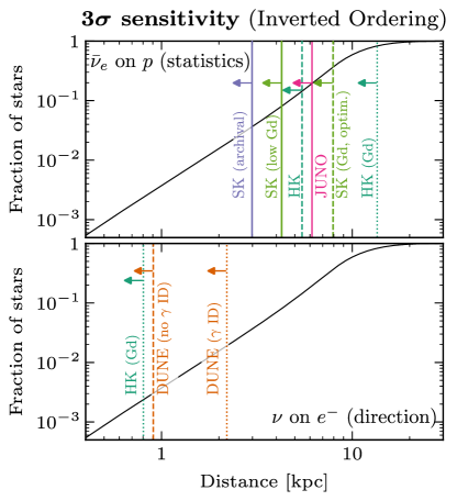
Figure E9: Same as Fig. 4, but assuming the inverted mass ordering.

References

- (1) B. Paczynski, Common Envelope Binaries, in Structure and Evolution of Close Binary Systems (P. Eggleton, S. Mitton, and J. Whelan, eds.), vol. 73, p. 75, Jan., 1976.
- (2) Z. Han, P. Podsiadlowski, and P. P. Eggleton, The formation of bipolar planetary nebulae and close white dwarf binaries, MNRAS 272 (Feb., 1995) 800–820.
- (3) K. Belczynski, S. Repetto, D. E. Holz, R. O’Shaughnessy, T. Bulik, E. Berti, C. Fryer, and M. Dominik, Compact Binary Merger Rates: Comparison with LIGO/Virgo Upper Limits, ApJ 819 (Mar., 2016) 108, [1510.04615].
- (4) T. Fragos, J. J. Andrews, E. Ramirez-Ruiz, G. Meynet, V. Kalogera, R. E. Taam, and A. Zezas, The Complete Evolution of a Neutron-Star Binary through a Common Envelope Phase Using 1D Hydrodynamic Simulations, Astrophys. J. Lett. 883 (2019), no. 2 L45, [1907.12573].
- (5) N. Ivanova, S. Justham, X. Chen, O. De Marco, C. L. Fryer, E. Gaburov, H. Ge, E. Glebbeek, Z. Han, X. D. Li, G. Lu, T. Marsh, P. Podsiadlowski, A. Potter, N. Soker, R. Taam, T. M. Tauris, E. P. J. van den Heuvel, and R. F. Webbink, Common envelope evolution: where we stand and how we can move forward, A&A Rev. 21 (Feb., 2013) 59, [1209.4302].
- (6) N. Ivanova, S. Justham, and P. Ricker, Common Envelope Evolution. IOP Publishing, 2020.
- (7) Y. B. Ginat, H. Glanz, H. B. Perets, E. Grishin, and V. Desjacques, Gravitational waves from in-spirals of compact objects in binary common-envelope evolution, Mon. Not. Roy. Astron. Soc. 493 (2020), no. 4 4861–4867, [1903.11072].
- (8) B. Hutilukejiang, C. Zhu, Z. Wang, and G. Lü, Formation of Thorne-Żytkow objects in close binaries, Journal of Astrophysics and Astronomy 39 (Apr., 2018) 21.
- (9) R. A. Chevalier, Neutron Star Accretion in a Supernova, ApJ 346 (Nov., 1989) 847.
- (10) J. C. Houck and R. A. Chevalier, Steady Spherical Hypercritical Accretion onto Neutron Stars, ApJ 376 (July, 1991) 234.
- (11) R. A. Chevalier, Neutron Star Accretion in a Stellar Envelope, ApJ 411 (July, 1993) L33.
- (12) P. M. Ricker and R. E. Taam, An AMR Study of the Common-envelope Phase of Binary Evolution, ApJ 746 (Feb., 2012) 74, [1107.3889].
- (13) M. MacLeod and E. Ramirez-Ruiz, On the Accretion-Fed Growth of Neutron Stars During Common Envelope, Astrophys. J. Lett. 798 (2015), no. 1 L19, [1410.5421].
- (14) M. MacLeod, A. Antoni, A. Murguia-Berthier, P. Macias, and E. Ramirez-Ruiz, Common Envelope Wind Tunnel: Coefficients of Drag and Accretion in a Simplified Context for Studying Flows around Objects Embedded within Stellar Envelopes, ApJ 838 (Mar., 2017) 56, [1704.02372].
- (15) S. L. Shapiro, Accretion onto Black Holes: the Emergent Radiation Spectrum, ApJ 180 (Mar., 1973) 531–546.
- (16) J. P. Cox and R. T. Giuli, Principles of stellar structure. Gordon and Breach, 1968.
- (17) L. Bildsten and A. Cumming, Hydrogen electron capture in accreting neutron stars and the resulting g-mode oscillation spectrum, Astrophys. J. 506 (1998) 842, [astro-ph/9807012].
- (18) Y. Egawa and K. Yokoi, Energy Loss Accompanying the Electron Captures in Highly Evolved Stars, Progress of Theoretical Physics 57 (Apr., 1977) 1255–1261.
- (19) B. Paxton, L. Bildsten, A. Dotter, F. Herwig, P. Lesaffre, and F. Timmes, Modules for Experiments in Stellar Astrophysics (MESA), ApJS 192 (jan, 2011) 3, [1009.1622].
- (20) B. Paxton, M. Cantiello, P. Arras, L. Bildsten, E. F. Brown, A. Dotter, C. Mankovich, M. H. Montgomery, D. Stello, F. X. Timmes, and R. Townsend, Modules for Experiments in Stellar Astrophysics (MESA): Planets, Oscillations, Rotation, and Massive Stars, ApJS 208 (sep, 2013) 4, [1301.0319].
- (21) B. Paxton, P. Marchant, J. Schwab, E. B. Bauer, L. Bildsten, M. Cantiello, L. Dessart, R. Farmer, H. Hu, N. Langer, R. H. D. Townsend, D. M. Townsley, and F. X. Timmes, Modules for Experiments in Stellar Astrophysics (MESA): Binaries, Pulsations, and Explosions, ApJS 220 (sep, 2015) 15, [1506.03146].
- (22) B. Paxton, J. Schwab, E. B. Bauer, L. Bildsten, S. Blinnikov, P. Duffell, R. Farmer, J. A. Goldberg, P. Marchant, E. Sorokina, A. Thoul, R. H. D. Townsend, and F. X. Timmes, Modules for Experiments in Stellar Astrophysics (MESA): Convective Boundaries, Element Diffusion, and Massive Star Explosions, ApJS 234 (feb, 2018) 34, [1710.08424].
- (23) B. Paxton, R. Smolec, J. Schwab, A. Gautschy, L. Bildsten, M. Cantiello, A. Dotter, R. Farmer, J. A. Goldberg, A. S. Jermyn, S. M. Kanbur, P. Marchant, A. Thoul, R. H. D. Townsend, W. M. Wolf, M. Zhang, and F. X. Timmes, Modules for Experiments in Stellar Astrophysics (MESA): Pulsating Variable Stars, Rotation, Convective Boundaries, and Energy Conservation, ApJS 243 (Jul, 2019) 10, [1903.01426].
- (24) A. S. Jermyn, E. B. Bauer, J. Schwab, R. Farmer, W. H. Ball, E. P. Bellinger, A. Dotter, M. Joyce, P. Marchant, J. S. G. Mombarg, W. M. Wolf, T. L. Sunny Wong, G. C. Cinquegrana, E. Farrell, R. Smolec, A. Thoul, M. Cantiello, F. Herwig, O. Toloza, L. Bildsten, R. H. D. Townsend, and F. X. Timmes, Modules for Experiments in Stellar Astrophysics (MESA): Time-dependent Convection, Energy Conservation, Automatic Differentiation, and Infrastructure, ApJS 265 (Mar., 2023) 15, [2208.03651].
- (25) F. J. Rogers and A. Nayfonov, Updated and Expanded OPAL Equation-of-State Tables: Implications for Helioseismology, ApJ 576 (Sept., 2002) 1064–1074.
- (26) D. Saumon, G. Chabrier, and H. M. van Horn, An Equation of State for Low-Mass Stars and Giant Planets, ApJS 99 (aug, 1995) 713.
- (27) A. W. Irwin, The FreeEOS Code for Calculating the Equation of State for Stellar Interiors, 2004.
- (28) F. X. Timmes and F. D. Swesty, The Accuracy, Consistency, and Speed of an Electron-Positron Equation of State Based on Table Interpolation of the Helmholtz Free Energy, ApJS 126 (feb, 2000) 501–516.
- (29) A. Y. Potekhin and G. Chabrier, Thermodynamic Functions of Dense Plasmas: Analytic Approximations for Astrophysical Applications, Contributions to Plasma Physics 50 (jan, 2010) 82–87, [1001.0690].
- (30) N. Itoh, H. Hayashi, A. Nishikawa, and Y. Kohyama, Neutrino Energy Loss in Stellar Interiors. VII. Pair, Photo-, Plasma, Bremsstrahlung, and Recombination Neutrino Processes, ApJS 102 (Feb., 1996) 411.
- (31) A. S. Clark, E. T. Johnson, Z. Chen, K. Eiden, D. E. Willcox, B. Boyd, L. Cao, C. J. DeGrendele, and M. Zingale, pynucastro: A Python Library for Nuclear Astrophysics, Astrophys. J. 947 (2023), no. 2 65, [2210.09965].
- (32) M. MacLeod and E. Ramirez-Ruiz, Asymmetric Accretion Flows within a Common Envelope, ApJ 803 (Apr., 2015) 41, [1410.3823].
- (33) L. D. Landau and E. M. Lifshitz, Fluid mechanics. Pergamon Press, 1959.
- (34) C. Kato, M. D. Azari, S. Yamada, K. Takahashi, H. Umeda, T. Yoshida, and K. Ishidoshiro, Pre-supernova neutrino emissions from ONe cores in the progenitors of core-collapse supernovae: are they distinguishable from those of Fe cores?, Astrophys. J. 808 (2015), no. 2 168, [1506.02358].
- (35) A. S. Dighe and A. Y. Smirnov, Identifying the neutrino mass spectrum from the neutrino burst from a supernova, Phys. Rev. D 62 (2000) 033007, [hep-ph/9907423].
- (36) T.-K. Kuo and J. T. Pantaleone, Neutrino Oscillations in Matter, Rev. Mod. Phys. 61 (1989) 937.
- (37) M. Maltoni and A. Y. Smirnov, Solar neutrinos and neutrino physics, Eur. Phys. J. A 52 (2016), no. 4 87, [1507.05287].
- (38) I. Esteban, M. C. Gonzalez-Garcia, M. Maltoni, T. Schwetz, and A. Zhou, The fate of hints: updated global analysis of three-flavor neutrino oscillations, JHEP 09 (2020) 178, [2007.14792].
- (39) V. Brdar and X.-J. Xu, Beyond tree level with solar neutrinos: Towards measuring the flavor composition and CP violation, Phys. Lett. B 846 (2023) 138255, [2306.03160].
- (40) P. Vogel and J. F. Beacom, Angular distribution of neutron inverse beta decay, anti-neutrino(e) + p — e+ + n, Phys. Rev. D 60 (1999) 053003, [hep-ph/9903554].
- (41) A. Strumia and F. Vissani, Precise quasielastic neutrino/nucleon cross-section, Phys. Lett. B 564 (2003) 42–54, [astro-ph/0302055].
- (42) Super-Kamiokande Collaboration, K. Abe et al., Solar Neutrino Measurements in Super-Kamiokande-IV, Phys. Rev. D 94 (2016), no. 5 052010, [1606.07538].
- (43) JUNO Collaboration, A. Abusleme et al., JUNO sensitivity to the annihilation of MeV dark matter in the galactic halo, JCAP 09 (2023) 001, [2306.09567].
- (44) JUNO Collaboration, F. An et al., Neutrino Physics with JUNO, J. Phys. G 43 (2016), no. 3 030401, [1507.05613].
- (45) J. A. Formaggio and G. P. Zeller, From eV to EeV: Neutrino Cross Sections Across Energy Scales, Rev. Mod. Phys. 84 (2012) 1307–1341, [1305.7513].
- (46) W. Castiglioni, W. Foreman, I. Lepetic, B. R. Littlejohn, M. Malaker, and A. Mastbaum, Benefits of MeV-scale reconstruction capabilities in large liquid argon time projection chambers, Phys. Rev. D 102 (2020), no. 9 092010, [2006.14675].
- (47) I. Iben, Jr. and M. Livio, Common envelopes in binary star evolution, Publ. Astron. Soc. Pac. 105 (1993) 1373–1406.
- (48) F. K. Roepke and O. De Marco, Simulations of common-envelope evolution in binary stellar systems: physical models and numerical techniques, 2212.07308.
- (49) K. S. Thorne and A. N. Zytkow, Stars with degenerate neutron cores. I. Structure of equilibrium models., ApJ 212 (Mar., 1977) 832–858.
- (50) C. L. Fryer, W. Benz, and M. Herant, The Dynamics and outcomes of rapid infall onto neutron stars, Astrophys. J. 460 (1996) 801, [astro-ph/9509144].
- (51) R. Popham, S. E. Woosley, and C. Fryer, Hyperaccreting black holes and gamma-ray bursts, Astrophys. J. 518 (1999) 356–374, [astro-ph/9807028].
- (52) G. E. Brown, C. H. Lee, and H. A. Bethe, Hypercritical advection dominated accretion flow, Astrophys. J. 541 (2000) 918, [astro-ph/9909132].
- (53) R. Narayan, T. Piran, and P. Kumar, Accretion Models of Gamma-Ray Bursts, ApJ 557 (Aug., 2001) 949–957, [astro-ph/0103360].
- (54) W. H. Lee, E. Ramirez-Ruiz, and D. Page, Dynamical evolution of neutrino-cooled accretion disks: Detailed microphysics, lepton-driven convection, and global energetics, Astrophys. J. 632 (2005) 421–437, [astro-ph/0506121].
- (55) W. H. Lee and E. Ramirez-Ruiz, Accretion modes in collapsars: prospects for grb production, Astrophys. J. 641 (2006) 961–971, [astro-ph/0509307].
- (56) G. E. Brown, Neutron Star Accretion and Binary Pulsar Formation, ApJ 440 (Feb., 1995) 270.
- (57) E. Moreno Méndez, D. López-Cámara, and F. De Colle, Dynamics of jets during the Common Envelope phase, Mon. Not. Roy. Astron. Soc. 470 (2017), no. 3 2929–2937, [1702.03293].
- (58) A. Murguia-Berthier, M. MacLeod, E. Ramirez-Ruiz, A. Antoni, and P. Macias, Accretion Disk Assembly During Common Envelope Evolution: Implications for Feedback and LIGO Binary Black Hole Formation, ApJ 845 (Aug., 2017) 173, [1705.04698].
- (59) L. Chamandy, A. Frank, E. G. Blackman, J. Carroll-Nellenback, B. Liu, Y. Tu, J. Nordhaus, Z. Chen, and B. Peng, Accretion in common envelope evolution, MNRAS 480 (Oct., 2018) 1898–1911, [1805.03607].
- (60) D. López-Cámara, F. De Colle, and E. Moreno Méndez, Self-regulating jets during the Common Envelope phase, Mon. Not. Roy. Astron. Soc. 482 (2019), no. 3 3646–3655, [1806.11115].
- (61) D. López-Cámara, E. Moreno Méndez, and F. De Colle, Disc formation and jet inclination effects in common envelopes, Mon. Not. Roy. Astron. Soc. 497 (2020), no. 2 2057–2065, [2004.04158].
- (62) E. Moreno Méndez, F. De Colle, D. L. Cámara, and A. Vigna-Gómez, Hypercritical accretion during common envelopes in triples leading to binary black holes in the pair-instability-supernova mass gap, 2207.03514.
- (63) Y. Sakurai, K. Inayoshi, and Z. Haiman, Hyper-Eddington mass accretion on to a black hole with super-Eddington luminosity, Mon. Not. Roy. Astron. Soc. 461 (2016), no. 4 4496–4504, [1605.09105].
- (64) K. Sugimura, T. Hosokawa, H. Yajima, and K. Omukai, Rapid Black Hole Growth under Anisotropic Radiation Feedback, Mon. Not. Roy. Astron. Soc. 469 (2017), no. 1 62–79, [1610.03482].
- (65) K. Rozwadowska, F. Vissani, and E. Cappellaro, On the rate of core collapse supernovae in the milky way, New Astron. 83 (2021) 101498, [2009.03438].
- (66) P. Podsiadlowski, R. C. Cannon, and M. J. Rees, The evolution and final fate of massive Thorne-Zytkow objects, MNRAS 274 (May, 1995) 485–490.
- (67) D. A. Dicus, Stellar energy-loss rates in a convergent theory of weak and electromagnetic interactions, Phys. Rev. D 6 (1972) 941–949.
- (68) E. Braaten and D. Segel, Neutrino energy loss from the plasma process at all temperatures and densities, Phys. Rev. D 48 (1993) 1478–1491, [hep-ph/9302213].
- (69) F. J. Fattoyev, E. F. Brown, A. Cumming, A. Deibel, C. J. Horowitz, B.-A. Li, and Z. Lin, Deep crustal heating by neutrinos from the surface of accreting neutron stars, Phys. Rev. C 98 (2018), no. 2 025801, [1710.10367].
- (70) S. W. Li and J. F. Beacom, First calculation of cosmic-ray muon spallation backgrounds for MeV astrophysical neutrino signals in Super-Kamiokande, Phys. Rev. C 89 (2014) 045801, [1402.4687].
- (71) S. W. Li and J. F. Beacom, Tagging Spallation Backgrounds with Showers in Water-Cherenkov Detectors, Phys. Rev. D 92 (2015), no. 10 105033, [1508.05389].
- (72) S. W. Li and J. F. Beacom, Spallation Backgrounds in Super-Kamiokande Are Made in Muon-Induced Showers, Phys. Rev. D 91 (2015), no. 10 105005, [1503.04823].
- (73) G. Zhu, S. W. Li, and J. F. Beacom, Developing the MeV potential of DUNE: Detailed considerations of muon-induced spallation and other backgrounds, Phys. Rev. C 99 (2019), no. 5 055810, [1811.07912].
- (74) JUNO Collaboration, A. Abusleme et al., JUNO physics and detector, Prog. Part. Nucl. Phys. 123 (2022) 103927, [2104.02565].
- (75) A. M. Ankowski, O. Benhar, T. Mori, R. Yamaguchi, and M. Sakuda, Analysis of -ray production in neutral-current neutrino-oxygen interactions at energies above 200 MeV, Phys. Rev. Lett. 108 (2012) 052505, [1110.0679].
- (76) T2K Collaboration, K. Abe et al., Measurement of the neutrino-oxygen neutral-current interaction cross section by observing nuclear deexcitation rays, Phys. Rev. D 90 (2014), no. 7 072012, [1403.3140].
- (77) Super-Kamiokande Collaboration, L. Wan et al., Measurement of the neutrino-oxygen neutral-current quasielastic cross section using atmospheric neutrinos at Super-Kamiokande, Phys. Rev. D 99 (2019), no. 3 032005, [1901.05281].
- (78) T2K Collaboration, K. Abe et al., Measurement of neutrino and antineutrino neutral-current quasielasticlike interactions on oxygen by detecting nuclear deexcitation rays, Phys. Rev. D 100 (2019), no. 11 112009, [1910.09439].
- (79) Super-Kamiokande Collaboration, K. Abe et al., Diffuse supernova neutrino background search at Super-Kamiokande, Phys. Rev. D 104 (2021), no. 12 122002, [2109.11174].
- (80) J. F. Beacom and M. R. Vagins, GADZOOKS! Anti-neutrino spectroscopy with large water Cherenkov detectors, Phys. Rev. Lett. 93 (2004) 171101, [hep-ph/0309300].
- (81) Super-Kamiokande Collaboration, M. Harada et al., Search for Astrophysical Electron Antineutrinos in Super-Kamiokande with 0.01% Gadolinium-loaded Water, Astrophys. J. Lett. 951 (2023), no. 2 L27, [2305.05135].
- (82) Hyper-Kamiokande Collaboration, K. Abe et al., Hyper-Kamiokande Design Report, 1805.04163.
- (83) DUNE Collaboration, B. Abi et al., Deep Underground Neutrino Experiment (DUNE), Far Detector Technical Design Report, Volume II: DUNE Physics, 2002.03005.
- (84) L. A. Girardi, M. A. T. Groenewegen, E. Hatziminaoglou, and L. da Costa, Star counts in the Galaxy. Simulating from very deep to very shallow photometric surveys with the TRILEGAL code, Astron. Astrophys. 436 (2005) 895–915, [astro-ph/0504047].
- (85) S. M. Adams, C. S. Kochanek, J. F. Beacom, M. R. Vagins, and K. Z. Stanek, Observing the Next Galactic Supernova, Astrophys. J. 778 (2013) 164, [1306.0559].
- (86) S. Ando, J. F. Beacom, and H. Yuksel, Detection of neutrinos from supernovae in nearby galaxies, Phys. Rev. Lett. 95 (2005) 171101, [astro-ph/0503321].
- (87) H.-L. Li, Y.-F. Li, L.-J. Wen, and S. Zhou, Prospects for Pre-supernova Neutrino Observation in Future Large Liquid-scintillator Detectors, JCAP 05 (2020) 049, [2003.03982].
- (88) JUNO Collaboration, A. Abusleme et al., Real-time Monitoring for the Next Core-Collapse Supernova in JUNO, 2309.07109.
- (89) Super-Kamiokande Collaboration, S. Locke et al., New Methods and Simulations for Cosmogenic Induced Spallation Removal in Super-Kamiokande-IV, 2112.00092.
- (90) F. Capozzi, S. W. Li, G. Zhu, and J. F. Beacom, DUNE as the Next-Generation Solar Neutrino Experiment, Phys. Rev. Lett. 123 (2019), no. 13 131803, [1808.08232].
- (91) J. F. Beacom and P. Vogel, Can a supernova be located by its neutrinos?, Phys. Rev. D 60 (1999) 033007, [astro-ph/9811350].
- (92) A. M. Holgado, P. M. Ricker, and E. A. Huerta, Gravitational Waves from Accreting Neutron Stars undergoing Common-Envelope Inspiral, Astrophys. J. 857 (2018), no. 1 38, [1706.09413].
- (93) J. D. Keegans, C. L. Fryer, S. W. Jones, B. Cote, K. Belczynski, F. Herwig, M. Pignatari, A. M. Laird, and C. A. Diget, Nucleosynthetic Yields from Neutron Stars Accreting in Binary Common Envelopes, 1902.01661.