Tight-binding theory of spin-spin interactions, Curie temperatures, and quantum Hall effects in topological (Hg,Cr)Te in comparison to non-topological (Zn,Cr)Te, and (Ga,Mn)N

Abstract

Earlier theoretical results on $p$-$d$ and $d$-$d$ exchange interactions for zinc-blende semiconductors with Cr²⁺ and Mn³⁺ ions are revisited and extended by including contributions beyond the dominating ferromagnetic (FM) superexchange term [i.e., the interband Bloembergen-Rowland-Van Vleck contribution and antiferromagnetic (AFM) two-electron term], and applied to topological Cr-doped HgTe and non-topological (Zn,Cr)Te and (Ga,Mn)N in zinc-blende and wurtzite crystallographic structures. From the obtained values of the $d$-$d$ exchange integrals $J_{ij}$, and by combining the Monte-Carlo simulations with the percolation theory for randomly distributed magnetic ions, we determine magnitudes of Curie temperatures $T_{\text{C}}(x)$ for $\mathrm{Zn}_{1-x}\mathrm{Cr}_{x}\mathrm{Te}$ and $\mathrm{Ga}_{1-x}\mathrm{Mn}_{x}\mathrm{N}$ and compare to available experimental data. Furthermore, we find that competition between FM and AFM $d$-$d$ interactions can lead to a spin-glass phase in the case of Hg_1-xCr_xTe. This competition, along with a relatively large magnitude of the AF $p$-$d$ exchange energy $N_{0}\beta$ can stabilize the quantum spin Hall effect, but may require the application of tilted magnetic field to observe the quantum anomalous Hall effect in HgTe quantum wells doped with Cr.

I Introduction

Extensive studies of (Ga,Mn)As and other dilute ferromagnetic semiconductors (DFSs), in which band holes mediate exchange interactions and magnetic anisotropies, have allowed demonstrating several functionalities, such as the effects of light, electric fields and currents on the magnetization magnitude and direction Dietl and Ohno (2014); Jungwirth et al. (2014). Similarly striking phenomena have been discovered in DFSs without band carriers, the prominent examples being the piezo-electro-magnetic effect in wurtzite (Ga,Mn)N Sztenkiel et al. (2016) or the parity anomaly Mogi et al. (2022) and the quantum anomalous Hall effect Yu et al. (2010); Chang et al. (2013) in topological (Bi,Sb,Cr)Te and related systems Ke et al. (2018); Tokura et al. (2019); Bernevig et al. (2022); Chang et al. (2023), the latter opening a prospect for developing a functional low magnetic field resistance standard Goetz et al. (2018); Fox et al. (2018); Okazaki et al. (2022); Rodenbach et al. (2023). In agreement with indications coming from synchrotron studies of magnetic configurations of V and Cr impurities in (Bi,Sb)₂Te₃ Peixoto et al. (2020), a theory developed by us for dilute magnetic semiconductors (DMS) such as topological (Hg,Mn)Te and topologically trivial (Cd,Mn)Te Śliwa et al. (2021) shows that, if a spurious self-interaction term is disregarded, the Anderson-Goodenough-Kanamori superexchange dominates over the interband Bloembergen-Rowland-Van Vleck mechanism Yu et al. (2010); Ke et al. (2018); Tokura et al. (2019); Bernevig et al. (2022); Chang et al. (2023) on the both sides of the topological phase transition in insulator magnetic systems Śliwa et al. (2021). Ferromagnetic insulators also serve to generate giant Zeeman splitting of bands in adjacent layers: the quantum anomalous Hall effect in (Bi,Sb)Te/(Zn,Cr)Te quantum wells (QWs) Watanabe et al. (2019) and topological superconductivity in InAs nanowires proximitized by an EuS layer Escribano et al. (2022) constitute just two recent examples.

Exchange interactions between the spins of electrons residing in partially occupied $d$-shells, mediated by hybridization $\hat{V}_{\text{hyb}}$ between $d$ shells of magnetic ions and $p$ orbitals of neighboring anions, can be either ferromagnetic (FM) or antiferromagnetic (AFM), orbital dependent, and sensitive to Jahn-Teller distortions Goodenough (1963). The progress in understanding the underlying mechanism of these interactions allowed to formulate Anderson-Goodenough-Kanamori rules Goodenough (1963), which predict the character of the interactions in a given system provided that the nature of the relevant chemical bonds is known. More recently, Blinowski, Kacman, and Majewski Blinowski et al. (1996) — by a tedious calculation involving the fourth-order perturbation theory in $\hat{V}_{\text{hyb}}$ — found that in tetrahedrally coordinated II-VI Cr-based dilute magnetic semiconductors the superexchange component of the spin pair interaction is FM. This FM coupling results from the partial filling of $t_{2}$ orbitals occurring for the high spin $d^{4}$ electronic configuration of the magnetic shell in the case of the substitutional $\mathrm{Cr}^{2{+}}$ ions in the tetrahedral environment. On the experimental side, FM ordering was indeed found in (Zn,Cr)Te but a meaningful determination of Curie temperature $T_{\text{C}}$ as a function of the Cr concentration $x$ is hampered by aggregation of Cr cations Kuroda et al. (2007a). Accordingly, the values of $T_{\text{C}}(x)$ determined recently for high quality $\mathrm{Zn}_{1-x}\mathrm{Cr}_{x}\mathrm{Te}$ epilayers Watanabe et al. (2019) provide an upper limit of $T_{\text{C}}$ expected for a random distribution of magnetic ions. The generality of the superexchange scenario was then demonstrated in the case of wurtzite (wz) (Ga,Mn)N containing randomly distributed $\mathrm{Mn}^{3{+}}$ ions, for which the experimental dependence $T_{\text{C}}(x)$ Sarigiannidou et al. (2006); Sawicki et al. (2012); Stefanowicz et al. (2013) was reasonably well explained theoretically employing Blinowski’s et al. theory for the zinc-blende structure. Monte-Carlo simulations served to obtain $T_{\text{C}}(x)$ magnitudes from the computed values of the exchange integrals $J_{ij}$ for Mn spin pairs at the distances $R_{ij}$ up to the 16th coordination sphere Sawicki et al. (2012); Stefanowicz et al. (2013); Simserides et al. (2014).

Here, the above-mentioned theoretical results for the $d^{4}$ configuration in DMS without band carriers are revisited and extended by including additional contributions beyond the superexchange, which results from the fourth order perturbation theory in $\hat{V}_{\text{hyb}}$, such as the interband Bloembergen-Rowland term Bloembergen and Rowland (1955); Lewiner et al. (1980); Larson et al. (1988); Dietl et al. (2001); Kacman (2001); Śliwa and Dietl (2018); Śliwa et al. (2021), known in the topological literature as the Van Vleck mechanism Yu et al. (2010); Ke et al. (2018); Tokura et al. (2019); Bernevig et al. (2022); Chang et al. (2023). Furthermore, our theory is developed for both zinc-blende and wurtzite semiconductors, allowing us to assess the crystal structure’s role in magnetic interactions. We also demonstrate quantitative agreement in the values of $T_{\text{C}}$ obtained by the Monte-Carlo simulations and from the percolation theory for random ferromagnets Korenblit et al. (1973). This agreement makes us possible to determine $T_{\text{C}}(x)$ from $J(R_{ij})$ values for the whole $x$ range, $0<x<1$, without Monte-Carlo simulations that are computationally expensive for disordered magnetic systems. The present developments are possible by making use of contemporary software tools for formula derivations, which allowed us to correct several inaccuracies in the original formulae Blinowski et al. (1996) for superexchange between pairs of spins residing on $d^{4}$ shells. We also correct some previous inconsistencies in values of Mn parameters Simserides et al. (2014) and discuss our results in comparison to experimental data on $T_{\text{C}}(x)$ for wz-$\mathrm{Ga}_{1-x}\mathrm{Mn}_{x}\mathrm{N}$ Sarigiannidou et al. (2006); Sawicki et al. (2012); Stefanowicz et al. (2013) and zb-(Zn,Cr)Te Watanabe et al. (2019).

Comparing the present results for Cr²⁺ and Mn³⁺ to the previously investigated Mn²⁺ case [realized in (Hg,Mn)Te and (Cd,Mn)Te] Śliwa et al. (2021), the superexchange term (denoted as $hh$) has the opposite sign for those two configurations. In contrast, the interband $he$ and $ee$ contributions behave similarly, i.e., $he$ is FM at small distances between magnetic ions and AFM for distant pairs. Our results demonstrate, in agreement with experimental observations, that FM interactions prevail in the case of (Zn,Cr)Te and wz-(Ga,Mn)N. At the same time, our $T_{\text{C}}$ values are much smaller compared to ab initio results Sato et al. (2010), as local functional approximations tend to underestimate localized character of $3d$ orbitals in semiconductors.

According to our theory, the ferromagnetic $hh$ term entirely dominates in (Ga,Mn)N. We show that the theoretical $T_{\text{C}}(x)$ magnitudes for wz-(Ga,Mn)Te are only slightly larger than experimental values, which may point out to an influence of the Jahn-Teller distortion neglected in the present approach.

However, the situation is more involved in the case of (Hg,Cr)Te and (Zn,Cr)Te. In those systems, due to the importance of the competition between FM and AFM couplings, the theoretically expected critical temperatures are rather sensitive to the employed tight-binding model of the host band structure. Actually, in the case of topological (Hg,Cr)Te, although the sign of Curie-Weiss temperatures points to a prevailing role of the FM interactions, a competition between FM and AFM contributions may result in the spin-glass freezing at low temperatures.

The striking properties of semiconductors with magnetic ions mentioned above result from strong $sp$-$d$ exchange interactions between effective mass carriers and electrons residing in open $d$ shells of magnetic ions Bonanni et al. (2021). While the signs and magnitudes of $s$-$d$ and $p$-$d$ exchange integrals have been extensively studied theoretically Kacman (2001); Dietl (2008) and experimentally Mac et al. (1996); Suffczyński et al. (2011) for wide band gap Cr-doped II-VI compounds and wz-(Ga,Mn)N, we present here theory of $sp$-$d$ coupling for Cr-doped topological HgTe. We show that the presence of Cr ions should improve the quantization accuracy of the quantum spin Hall effect in the paramagnetic phase. We also enquire on whether the quantum anomalous Hall effect, examined so far theoretically for Mn-doped HgTe QWs Liu et al. (2008a), could be observed in the Cr-doping case.

II Impurity and band structure parameter values

II.1 Cr and Mn impurity levels

We place zero energy at the valence band top. We are interested in three energy levels introduced by cation-substitutional $\mathrm{Cr}$ impurities in II-VI compounds (HgTe and ZnTe) and $\mathrm{Mn}$ impurities in GaN: (i) the donor level $E_{d}$ corresponding to $\mathrm{Cr}^{2{+}/3{+}}$ and $\mathrm{Mn}^{3{+}/4{+}}$ states with the spin $S=2$; (ii) two acceptor states of $\mathrm{Cr}^{2{+}/1{+}}$ and $\mathrm{Mn}^{3{+}/2{+}}$ located at energies $E_{d}+U$ and $E_{d}+U+J$ corresponding to five $d$ electrons but different spin value, $S=5/2$ and $S=3/2$, respectively. Spectroscopic free-ion data imply the exchange energy $J=3$ eV Blinowski et al. (1996). Experimental studies of ZnTe:Cr point to $E_{d}=0.2$ eV and $U=1.1$ eV Kuroda et al. (2007b). Assuming the valence band offset between HgTe and ZnTe $W=0.5$ eV, we anticipate $E_{d}=-0.3\pm 0.1$ eV in HgTe:Cr. Similarly, experimental results for wz-GaN:Mn lead to $E_{d}=1.1$ eV and $U=0.7$ eV Graf et al. (2003); Han et al. (2005); Hwang et al. (2005). (In Ref. Simserides et al., 2014 $E_{d}=1.8$ eV was incorrectly used). Because of the lack of reliable data for the internal strain parameter $u$, we assume that Cr and Mn impurities are located at the center of the tetrahedron of the nearest-neighbor anions; the distortion due to Jahn-Teller effect is neglected.

Table 1: Summary of the electronic configurations involved in the leading order of perturbation theory for a $d^{4}$ ground state and spherical symmetry.

Configuration	Number of electrons	Spin	Orbital angular momentum	Energy (Parmenter)	Total degeneracy
$d^{3}$	3	$3/2$	1, 3	$3E_{0}-3J+3U$	40
$d^{4}$	4	2	2	$4E_{0}-6J+6U$	25
$d^{5}$	5	$5/2$	0	$5E_{0}-10J+10U$	6
$d^{5\downarrow}$	5	$3/2$	1, 2, 3, 4	$5E_{0}-5J+10U$	96

II.2 Tight-binding parameters

One of standard approaches to determine electronic energy bands in solids is the tight-binding approximation (TBA). Within that model, empirical or ab initio data provide on-site and overlap energies which serve to construct the Bloch Hamiltonian. We reuse the $sp^{3}$ band structure parameters given previously for HgTe Śliwa et al. (2021). together with $V_{pd\sigma}=-0.64\,\mathrm{eV}$, $V_{pd\pi}=-0.45V_{pd\sigma}$, and $V_{sd\sigma}=1.08V_{ps\sigma}$ for Cr ions Blinowski et al. (1996). The tight-binding parameters of Ref. Bertho et al., 1991 are employed for ZnTe. For zb-GaN we reuse the parameter set of Ref. Simserides et al., 2014, whereas a set of parameters published by Yang et al. have been employed for wz-GaN, although we include all the second-neighbor overlaps (only half of them have been originally included). We neglect possible inconsistencies in the parameter set that may arise as a result.

In order to verify whether the present results are sensitive to details of the band-structure, additional models have been considered for (Hg,Cr)Te and (Zn,Cr)Te. These models include explicitly the $d$ orbitals of both the cation and anion, thus allowing to include also $d$-$d$ hybridization. In the band-structure models which include the $d$ orbitals of the anion we assume for the hybridization matrix elements, following the universal ratios of tight-binding overlaps Shi and Papaconstantopoulos (2004): $V_{dd\sigma}=-3.47\,\mathrm{eV}$, $V_{dd\pi}=1.87\,\mathrm{eV}$, and $V_{dd\delta}=-0.51\,\mathrm{eV}$.

III Theory of spin-spin interactions

We follow the established approach Larson et al. (1988); Śliwa and Dietl (2018); Śliwa et al. (2021) based on the leading-order perturbation theory (4th-order in $p$-$d$ hybridization). We use here the convention for the Hamiltonian representing spin pair interactions, $H_{ij}=-2J_{ij}\mathbf{S}_{i}\cdot\mathbf{S}_{j}$, where $J_{ij}$ results from angular averaging and, in general, contains three contributions, $hh$ corresponding to superexchange, $he$ describing the interband Bloembergen-Rowland coupling mechanism, and $ee$ giving the two-electron contribution. We adapt here our previous theory Śliwa et al. (2021) for the $d^{5}$ magnetic shells for the $d^{4}$ case.

The components of the full the Hamiltonian,

$$\hat{H}=(\hat{H}_{k}+\hat{H}_{d})+\hat{V}_{\text{hyb}},$$ (1)

correspond to a set of bands for non-interacting electrons ($\hat{H}_{k}=\sum_{k}E_{k}a_{k}^{\dagger}a_{k}$), the $d$-shells with the on-site Coulomb repulsion ($\hat{H}_{d}=\sum_{i}\hat{H}_{d,i}$, e.g., Parmenter’s Hamiltonians Parmenter (1973)), and hybridization between the band states and the $d$-shells ($\hat{V}_{\text{hyb}}$). Application of the perturbation theory involves summing over processes in which the electron jumps from one $d$-shell (state $d_{1}$) to a band state ($k$), then to the $d$-shell of another magnetic ion (state $d_{2}$), then to another band state ($k^{\prime}$), and then back to state $d_{1}$ — forming a closed path. Terms consisting of two independent loops (performed by two electrons) cancel in the total result. One has also to take into account, by means of the quasi-degenerate perturbation theory Winkler (2003), that we are interested in the Hamiltonian just for the ground state of the two magnetic ions, $d^{4}\otimes d^{4}$. Each term is a product of a phase due to the anticommutation rule for the fermionic creation and annihilation operators, an energetic denominator, and four matrix elements of the hybridization operator (the latter independent of the occupations of the band states or the order in which the transitions happen). We write the matrix elements of the effective Hamiltonian (between the initial and final states) as:

$$\left<d_{fin,1},d_{fin,2}\middle|H_{eff}^{(4)}\middle|d_{ini,1},d_{ini,2}\right>$$ (2)

$$= \sum_{k,k^{\prime}}\sum_{d_{int,1},d_{int,2}}A_{x_{1},x_{2}}(E_{k},E_{k^{\prime}},\mu)$$

$${}\times\left<d_{fin,1}\middle|a_{d,1,x_{1}}(k,k^{\prime})\middle|d_{int,1}\right>$$

$${}\times\left<d_{int,1}\middle|a_{d,1,x_{1}}(k^{\prime},k)^{\dagger}\middle|d_{ini,1}\right>$$

$${}\times\left<d_{fin,2}\middle|a_{d,2,x_{2}}(k^{\prime},k)\middle|d_{int,2}\right>$$

$${}\times\left<d_{int,2}\middle|a_{d,2,x_{2}}(k,k^{\prime})^{\dagger}\middle|d_{ini,2}\right>$$

Here, $x_{i}\in\{{+1},{-1}\}$ is ${+1}$ for acceptor excitations (intermediate state $d_{int,i}\in d^{5}\oplus d^{5\downarrow}$, see below) or ${-1}$ for donor excitations ($d_{int,i}\in d^{3}$), and $a_{d,i,x_{i}}(k,k^{\prime})$ is an annihilation [$a_{d,i,{+1}}(k,k^{\prime})=a_{d,i}(k)$] or creation [$a_{d,i,{-1}}(k,k^{\prime})=a_{d,i}(k^{\prime})^{\dagger}$] operator for the $d$-shell $i$, respectively. By definition, the hybridization operator can be written as the following sum over band states $k$:

$$\hat{V}_{\text{hyb}} = \sum_{i,k}[a_{k}^{\dagger}a_{d,i}(k)+a_{d,i}(k)^{\dagger}a_{k}],$$ (3)

$$a_{d,i}(k) = \sum_{n,s,m}\left<k\middle|n,s\right>\left<n\middle|V\middle|d,i,m\right>_{\kappa(k)}$$ (4)

$$\qquad{}\times e^{-i\kappa(k)\cdot\mathbf{R}_{i}}a_{d,i,m,s},$$

where $n$ is a band orbital index, $s\in\{\frac{1}{2},-\frac{1}{2}\}$ is a spin index, $m$ is a $d$-shell orbital index, and $\left<n\middle|V\middle|d,i,m\right>_{\kappa(k)}$ is the tight-binding overlap [at the wave vector $\kappa(k)$ corresponding to band state $k$] between band orbital $n$ and $d$-shell orbital $m$, the latter located at position $\mathbf{r}_{i}$ inside the unit cell, and at absolute position $\mathbf{R}_{i}=n_{1}\mathbf{a}_{1}+n_{2}\mathbf{a}_{2}+n_{3}\mathbf{a}_{3}+\mathbf{r}_{i}$ [$(n_{\alpha})_{\alpha=1,2,3}$ number lattice cells]. The phase factor $e^{-i\kappa(k)\cdot\mathbf{R}_{i}}$ compensates the fact that we are working with Bloch functions (rather than with wave functions).

The relevant subspace of the Hilbert space for the $d$-shells is a direct sum of the subspaces corresponding to the electronic configurations being involved in the leading order: $d^{4}$ (ground state), $d^{3}$, $d^{5}$ (high-spin) and $d^{5\downarrow}$ (spin-flipped). Since even in a tetrahedral symmetry this amounts to a 32-parameter Hamiltonian, we are virtually forced to reuse the three-parameter Hamiltonian of Parmenter Parmenter (1973). The relevant energies are given in terms of Parmenter’s $E_{0}$, $U$, $J$ in Table 1. We will denote as $E_{d}-E_{v}$, $E_{d}+U-E_{v}$, and $E_{d}+U+J-E_{v}$ the energies of the transitions $d^{3}\to d^{4}+h$, $d^{4}\to d^{5}+h$, $d^{4}\to d^{5\downarrow}+h$ (respectively; $h$ stands for a hole at the valence-band top, and $E_{v}$ for the valence-band-top energy).

Explicit expressions for $A$’s (including the phase factors) can be written for $d^{3}$ and $d^{5}$ excitations in an insulator ($E_{k}<E_{F}$ or $E_{k}>E_{F}$) in the low-temperature limit, $T\to 0^{+}$, $\mu\to E_{F}$, $f(E_{k})\to\Theta(E_{F}-E_{k})$, under the assumption that the ground state of the unperturbed Hamiltonian ($H_{k}+H_{d}$) corresponds to $d^{4}$ electronic configuration, i.e., $E_{d}<E_{F}$, $E_{d}+U>E_{F}$, and $E_{d}+U+J>E_{F}$ (the expression for $d^{5\downarrow}$ excitations are obtained by replacing $U$ with $U+J$ for the corresponding shell $d_{i}$; zero denominators, e.g. $E_{d,1}-E_{d,2}$, must be eliminated by taking appropriate limits: $E_{d,1},E_{d,2}\to E_{d}$, and/or formal algebraic transformations).

Table 2: A summary of the reduced matrix elements for the $d$-shells annihilation operators; cf. Eqs. (11–12).

$n$	$S$	$L$	$S^{\prime}$	$L^{\prime}$	$\left|\left<\left<a\right>\right>_{L,S;L^{\prime},S^{\prime}}\right|^{2}$
3	$3/2$	1	2	2	$6/5$
3	$3/2$	3	2	2	$14/5$
4	2	2	$5/2$	0	5
4	2	2	$3/2$	1	$5/4$
4	2	2	$3/2$	2	$5/4$
4	2	2	$3/2$	3	$5/4$
4	2	2	$3/2$	4	$5/4$

$$A_{+1,+1} = \frac{1}{2}\frac{f(E_{k})-f(E_{k^{\prime}})}{E_{k}-E_{k^{\prime}}}[w_{1u}(E_{k})w_{2u}(E_{k})+w_{1u}(E_{k^{\prime}})w_{2u}(E_{k^{\prime}})]+$$ (5)

$${}-\frac{1}{2}[f(E_{k})+f(E_{k^{\prime}})]\frac{w_{1u}(E_{k})w_{1u}(E_{k^{\prime}})-w_{2u}(E_{k})w_{2u}(E_{k^{\prime}})}{E_{d1}+U_{1}-E_{d2}-U_{2}}$$

$$A_{+1,-1} = \frac{1}{2}\frac{f(E_{k})-f(E_{k^{\prime}})}{E_{k}-E_{k^{\prime}}}[w_{1u}(E_{k})w_{2}(E_{k})+w_{1u}(E_{k^{\prime}})w_{2}(E_{k^{\prime}})]+$$ (6)

$${}-\frac{1}{2}[f(E_{k})+f(E_{k^{\prime}})]\frac{w_{1u}(E_{k})w_{1u}(E_{k^{\prime}})-w_{2}(E_{k})w_{2}(E_{k^{\prime}})}{E_{d1}+U_{1}-E_{d2}}+{}$$

$${}-\frac{w_{2}(E_{k})w_{2}(E_{k^{\prime}})}{E_{d1}+U_{1}-E_{d2}}$$

$$A_{-1,+1} = \frac{1}{2}\frac{f(E_{k})-f(E_{k^{\prime}})}{E_{k}-E_{k^{\prime}}}[w_{1}(E_{k})w_{2u}(E_{k})+w_{1}(E_{k^{\prime}})w_{2u}(E_{k^{\prime}})]+$$ (7)

$${}-\frac{1}{2}[f(E_{k})+f(E_{k^{\prime}})]\frac{w_{1}(E_{k})w_{1}(E_{k^{\prime}})-w_{2u}(E_{k})w_{2u}(E_{k^{\prime}})}{E_{d1}-E_{d2}-U_{2}}+{}$$

$${}+\frac{w_{1}(E_{k})w_{1}(E_{k^{\prime}})}{E_{d1}-E_{d2}-U_{2}}$$

$$A_{-1,-1} = \frac{1}{2}\frac{f(E_{k})-f(E_{k^{\prime}})}{E_{k}-E_{k^{\prime}}}[w_{1}(E_{k})w_{2}(E_{k})+w_{1}(E_{k^{\prime}})w_{2}(E_{k^{\prime}})]+$$ (8)

$${}-\frac{1}{2}[f(E_{k})+f(E_{k^{\prime}})]\frac{w_{1}(E_{k})w_{1}(E_{k^{\prime}})-w_{2}(E_{k})w_{2}(E_{k^{\prime}})}{E_{d1}-E_{d2}}+{}$$

$${}+\frac{w_{1}(E_{k})w_{1}(E_{k^{\prime}})-w_{2}(E_{k})w_{2}(E_{k^{\prime}})}{E_{d1}-E_{d2}}$$

$$w_{i}(E) = \frac{1}{E_{di}-E}$$ (9)

$$w_{iu}(E) = \frac{1}{E_{di}+U_{i}-E}$$ (10)

Matrix elements of the annihilation operators from $d^{n+1}$ to $d^{n}$ can be written in terms of Clebsch-Gordan coefficients as:

$$\left<d^{n},\alpha,L,S,L_{z,f},S_{z,f}\middle|a_{L_{z,a},S_{z,a}}\middle|d^{n+1},\beta,L^{\prime},S^{\prime},L_{z,i},S_{z,i}\right>={}$$ (11)

$$\left<\left<a\right>\right>_{\alpha,L,S;\beta,L^{\prime},S^{\prime}}\left<L^{\prime},L_{z,i}\middle|L,L_{z,f};2,L_{z,a}\right>\left<S^{\prime},S_{z,i}\middle|S,S_{z,f};\frac{1}{2},S_{z,a}\right>,$$

where $(L_{z,a},S_{z,a})$ are the quantum numbers of the annihilated electron. Analogously, we have for matrix elements of the creation operators from $d^{n}$ to $d^{n+1}$:

$$\left<d^{n+1},\alpha,L,S,L_{z,f},S_{z,f}\middle|a^{\dagger}_{L_{z,c},S_{z,c}}\middle|d^{n},\beta,L^{\prime},S^{\prime},L_{z,i},S_{z,i}\right>={}$$ (12)

$$\left<\left<a^{\dagger}\right>\right>_{\alpha,L,S;\beta,L^{\prime},S^{\prime}}\left<L,L_{z,f}\middle|L^{\prime},L_{z,i};2,L_{z,c}\right>\left<S,S_{z,f}\middle|S^{\prime},S_{z,i};\frac{1}{2},S_{z,c}\right>,$$

with $\left<\left<a^{\dagger}\right>\right>_{\alpha,L,S;\beta,L^{\prime},S^{\prime}}=\left<\left<a\right>\right>_{\beta,L^{\prime},S^{\prime};\alpha,L,S}^{*}$. The squared absolute values of the reduced matrix elements are summarized in Table 2.

Table 3: Values of $j_{m,m_{i}}(d_{sub,i})$ in equations (13) and (14) for an excitation with an orbital quantum number $m$ from a $d^{4}$ ground state with an orbital configuration $m_{i}$ (rows correspond to sectors of the Hilbert space) under spherical symmetry.

$d_{sub,i}$	$m=m_{i}$	$m\neq m_{i}$
$d^{3}$	0	$1/4$
$d^{5}$	$1/5$	0
$d^{5\downarrow}$	$-1/5$	$-1/4$

We further restrict our attention to the case when the orbital configurations $m_{i}$ of the $d$-shells remain unchanged. In such a situation an excitation (electron or hole) which enters the $d$-shell with an orbital quantum number $m$, leaves it with $m$ unchanged. Then, the spin-dependent parts of the subexpressions

$$\sum_{d_{int,i}\in d_{sub,i}}\left<d_{fin,i}\middle|a_{d,i,m,s}\middle|d_{int,i}\right>\left<d_{int,i}\middle|a_{d,i,m,s^{\prime}}^{\dagger}\middle|d_{ini,i}\right>$$ (13)

$$\cong j_{m,m_{i}}(d_{sub,i})\sum_{\alpha}\left<d_{fin,i}\middle|S_{i,\alpha}\middle|d_{ini,i}\right>\left<s\middle|\sigma_{\alpha}\middle|s^{\prime}\right>,\qquad$$

$$\sum_{d_{int,i}\in d_{sub,i}}\left<d_{fin,i}\middle|a_{d,i,m,s}^{\dagger}\middle|d_{int,i}\right>\left<d_{int,i}\middle|a_{d,i,m,s^{\prime}}\middle|d_{ini,i}\right>$$ (14)

$$\cong j_{m,m_{i}}(d_{sub,i})\sum_{\alpha}\left<d_{fin,i}\middle|S_{i,\alpha}\middle|d_{ini,i}\right>\left<s^{\prime}\middle|\sigma_{\alpha}\middle|s\right>,\qquad$$

and $j_{m,m_{i}}(d_{sub,i})$ are constant numbers which depend on the Hilbert subspace, $d_{sub,i}$, and the relation between the orbital quantum number $m$ and the orbital state of the $d$-shell, $m_{i}$, as summarized in Table 3.

Equipped with the results (5–8) and Table 3, we rederive Eqs. 1–9 of Ref. Blinowski et al., 1996, and find an incorrect normalization (the prefactor 2 in Eq. 1 of Ref. Blinowski et al., 1996 is extraneous), wrong signs of $F$ and $H$, a missing 2 in the numerator of $1/(e_{2}+e_{1})$ in $\mathcal{F}$, and a lacking symmetrization of $\mathcal{H}$ with respect to $\nu\leftrightarrow\nu^{\prime}$ (the last issue does not affect numerical values). Still, the numbers (e.g. for ZnTe:Cr) in Table I of Ref. Blinowski et al., 1996 are $-1/2$ the values that can be obtained from the incorrect formulas. However, as show in the next section, those corrections to the $hh$ contribution, together with $he$ and $ee$ terms taken into account here but neglect previously, while important quantitatively, do not alter the main conclusion of the previous works Blinowski et al. (1996); Simserides et al. (2014): spin-spin interactions are predominately FM for magnetic ions with high spin $d^{4}$ configuration in zinc-blende DMSs.

Even though the energy shifts due to Jahn-Teller effect are not taken into account in the present theory, the exchange integrals are sensitive to orbital configurations. We report as $J$ its average over the three $T_{2}$ states of each of the two $d$-shells in question (with an appropriate transformation of the quantization axis in the wurtzite case, as described in Appendix A).

Another challenge of the theory is the double integration over the Brillouin zone, particularly in the case of the interband $he$ term in zero-gap HgTe, where a singularity appears at $k,k^{\prime}\rightarrow 0$. We follow the procedure elaborated previously Śliwa et al. (2021), which involves a shift of the $k^{\prime}$ grid by different $\vartheta$ values. The number of $k$ and $\vartheta$ values employed here insures convergence of the results.

IV Numerical values of the exchange integrals

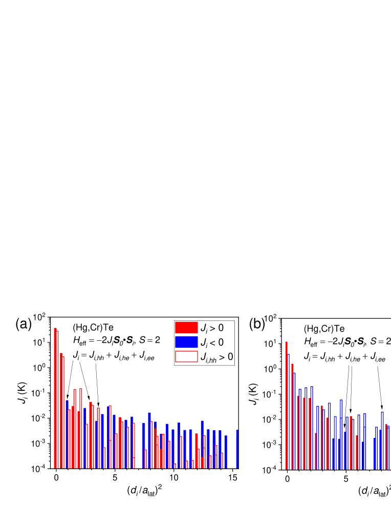
Figure 1: Exchange integrals $J_{i}$ in a logarithmic scale for spin pairs at distances $d_{i}$ corresponding to the first thirty cation coordination spheres $1\leq i\leq 30$, $d_{i}=(i/2)^{1/2}a_{\text{lat}}$ in zinc-blende topological (Hg,Cr)Te. (a) The total exchange energies and the superexchange ($hh$) contribution; (b) the remaining contributions: the electron-hole (Bloembergen-Rowland) and two-electron terms ($he$ an $ee$, respectively). Red and blue colors correspond to the FM and AFM sign of the interaction, respectively. As demonstrated elsewhere in the context of (Hg,Mn)Te Śliwa et al. (2021), the self-interaction terms at $d_{i}=0$ do not contribute to spin-spin exchange energies but account for a sizable overestimation of the interband contribution $he$ to the Curie temperature $T_{\text{C}}$, if evaluated in terms of the interband Van Vleck susceptibility Yu et al. (2010).

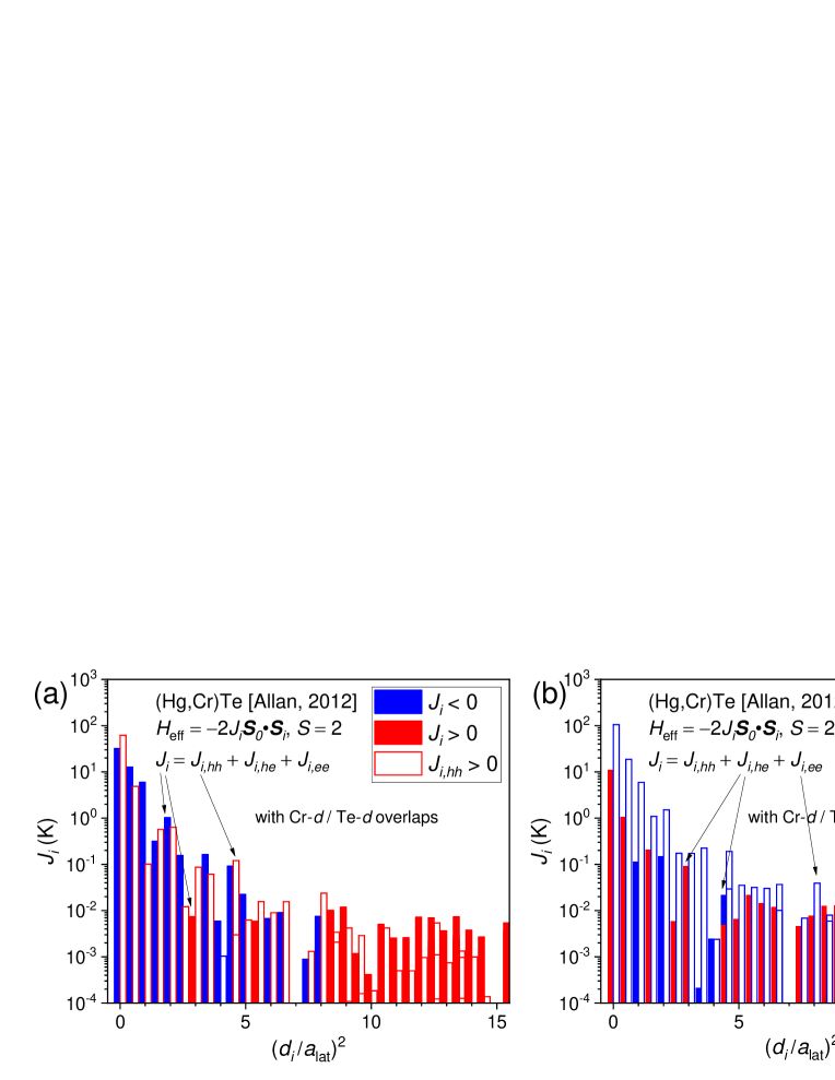
Figure 2: Exchange integrals $J_{i}$ in zinc-blende topological (Hg,Cr)Te according to the band-structure model of Ref. Allan and Delerue, 2012 (2048 $k$-points, 64 $\theta$-points).

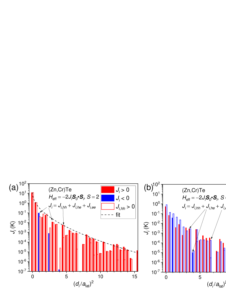
Figure 3: Same as in Fig.1 but for topologically trivial zinc-blende (Zn,Cr)Te.

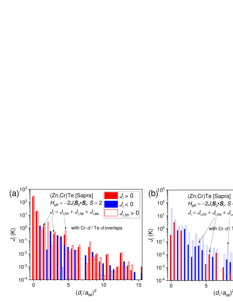
Figure 4: Exchange integrals $J_{i}$ in zinc-blende topologically trivial (Zn,Cr)Te according to the band-structure model of Ref. Sapra et al., 2002 (without second neighbor interactions; 16384 $k$-points).

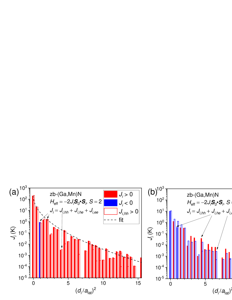
Figure 5: Same as in Fig.1 but for for topologically trivial zinc-blende (Ga,Mn)N.

We report our results in the convention according to which the Hamiltonian $H_{ij}$ for a pair $(i,j)$ is

$$H_{ij}=-2J_{ij}\mathbf{S}_{i}\cdot\mathbf{S}_{j},$$ (15)

where $\mathbf{S}_{i}$ and $\mathbf{S}_{j}$ are the quantum operators for $S=2$ spins. We present, in Figs. 1– 5 for (Hg,Cr)Te, (Zn,Cr)Te, and zb-(Ga,Mn)N, respectively the determined values of $J_{ij}\equiv J_{i}$ vs. the spin pair distance $R_{ij}\equiv d_{i}$, where $d_{i}=(i/\sqrt{2})a_{\text{lat}}$ denote the positions of the sequential cation coordination spheres and the lattice parameters $a_{\text{lat}}=0.646$ and $0.610$ nm for HgTe and ZnTe, respectively. Since the magnitudes of $J_{ij}$ decay exponentially with $d_{i}$, only the first few $J_{ij}$ values are significant and, therefore, shown in Tables 4–7 for the same systems and wz-(Ga,Mn)N.

Figure 6: Exchange integrals $J_{i}$ in a logarithmic scale for spin pairs at distances $R_{i}<1\,\mathrm{nm}$ in topologically-trivial wurtzite (Ga,Mn)N. See the caption of Fig.1 for the legend.

Table 4: $(\mathrm{Hg},\mathrm{Cr})\mathrm{Te}$: Numerical values of the total pair exchange integrals $J_{i}$ and contributions $hh$, $he$, and $ee$ for the nearest cation coordination zones located at distances $d_{i}=\sqrt{i/2}a_{\text{lat}}$ and containing $z_{i}$ cations. Positive and negative signs of $J$ correspond to FM and AFM coupling, respectively. The computations have been performed for 16384 $k$-points and 512 $\theta$-points (see, Sec. III and Ref. Śliwa et al., 2021).

$i$	$J_{i}(\mathrm{K})$	$J_{i,hh}(\mathrm{K})$	$J_{i,he}(\mathrm{K})$	$J_{i,ee}(\mathrm{K})$	$z_{i}$
1	$3.6631$	$2.7219$	$1.6255$	$-0.6843$	12
2	$-0.0496$	$0.0217$	$0.0857$	$-0.1570$	6
3	$0.0292$	$0.1371$	$0.0730$	$-0.1809$	24
4	$0.0185$	$0.1489$	$0.0707$	$-0.2011$	12

Table 5: Same as in Table 4 but for zb-(Zn,Cr)Te (16384 $k$-points).

$i$	$J_{i}(\mathrm{K})$	$J_{i,hh}(\mathrm{K})$	$J_{i,he}(\mathrm{K})$	$J_{i,ee}(\mathrm{K})$	$z_{i}$
1	$1.0936$	$1.1579$	$0.0687$	$-0.1330$	12
2	$-0.0967$	$0.0402$	$-0.0384$	$-0.0985$	6
3	$0.0366$	$0.0765$	$0.0040$	$-0.0438$	24
4	$0.0588$	$0.0734$	$0.0082$	$-0.0228$	12

Table 6: Same as in Table 4 but for zb-(Ga,Mn)N (16384 $k$-points).

$i$	$J_{i}(\mathrm{K})$	$J_{i,hh}(\mathrm{K})$	$J_{i,he}(\mathrm{K})$	$J_{i,ee}(\mathrm{K})$	$z_{i}$
1	$19.879$	$20.579$	$1.289$	$-1.989$	12
2	$-0.884$	$0.788$	$-0.386$	$-1.286$	6
3	$1.440$	$1.725$	$0.345$	$-0.630$	24
4	$1.629$	$1.625$	$0.326$	$-0.321$	12

Table 7: Same as Table 4 but for wz-(Ga,Mn)N (1152 $k$-points per unit cell of the reciprocal lattice).

$i$	$R_{i}(\text{\AA})$	$J_{i}(\mathrm{K})$	$J_{i,hh}(\mathrm{K})$	$J_{i,he}(\mathrm{K})$	$J_{i,ee}(\mathrm{K})$	$z_{i}$
1	$3.180$	$19.498$	$20.166$	$0.325$	$-0.988$	6
2	$3.189$	$18.898$	$19.859$	$0.729$	$-1.690$	6
3	$4.503$	$0.158$	$1.309$	$-0.101$	$-1.050$	6
4	$5.185$	$2.704$	$3.034$	$0.449$	$-0.779$	2
5	$5.518$	$1.272$	$1.519$	$0.250$	$-0.497$	12
6	$5.524$	$1.944$	$2.113$	$0.430$	$-0.599$	6
7	$6.087$	$1.186$	$1.487$	$0.120$	$-0.421$	12
8	$6.378$	$2.376$	$2.420$	$0.361$	$-0.405$	6

Another relevant quantity is the Curie-Weiss parameter,

$$\Theta_{0}=\frac{2}{3}\sum_{i\geq 1}z_{i}J_{i}S(S+1),$$ (16)

where $z_{i}$ is the number of cations in the $i$-th coordination sphere. In terms of $\Theta_{0}$ and according to the high-temperature expansion Spałek et al. (1986), Curie-Weiss temperature [equal to Curie temperature $T_{\text{C}}$ in the mean-field approximation (MFA)], is given by $\Theta_{\text{CW}}=x\Theta_{0}$, if a dependence of the band structure parameters on fractional magnetic cation content $x$ can be neglected. The values of $\Theta_{\text{CW}}$ for $x=0.1$ are shown in Table 8 for the studied systems.

Table 8: Curie-Weiss temperatures $\Theta_{\text{CW}}$ equivalent to Curie temperatures $T_{\text{C}}$ within the mean-field approximation compared to $T_{\text{C}}$ values obtained by Monte-Carlo (MC) simulations and the percolation (perc) theory (see Sec. V) for the systems under study with 10% cations substituted by magnetic impurities.

compound	$\Theta_{\text{CW}}$ (K)	$T_{\text{C}}^{\text{MC}}$ (K)	$T_{\text{C}}^{\text{perc}}$ (K)
zb-Hg0.9Cr0.1Te	$15.3$	–	–
zb-Hg0.9Cr0.1Te [Allan]	$-86.0$	–	–
zb-Zn0.9Cr0.1Te	$5.90$	$0.75$	$1.50$
zb-Zn0.9Cr0.1Te [Sapra]	$92.0$	–	–
zb-Ga0.9Mn0.1N	$123.8$	$28$	$30.1$
wz-Ga0.9Mn0.1N	$129.1$	$32$	$31.3$

Several conclusions emerge from the results displayed in Figs. 1–6 and Tables 4–8. First, as shown previously Śliwa et al. (2021), within the Van Vleck susceptiblity model Yu et al. (2010), $T_{\text{C}}^{(VV)}=x\Theta_{0}^{(VV)}$, where $\Theta_{0}^{(VV)}$ involves the summation only over $J_{i,he}$ and includes the self-interaction $J_{0,he}$ term with $z_{0}=1$. Since this spurious $J_{0,he}$ term is quite large, its inclusion with a simultaneous disregarding of superexchange (the $hh$ term), leads to the improper conclusion about the dominant role of the Van Vleck mechanism. Second, judging from the $\Theta_{0}$ values, FM interactions are about an order of magnitude stronger in both zb- and wz-(Ga,Mn)N compared to (Hg,Cr)Te and (Zn,Cr)Te. Within our model, this fact results from a short lattice constant of GaN leading to sizable $pd$ hybridization and a rather large magnitude of $J_{1}$, as found by ab initio studies and experimentally Bonanni et al. (2011). Third, AFM $ee$ term is surprisingly large in the case of (Hg,Cr)Te and (Zn,Cr)Te pointing to a possible competition between spin-glass and FM ordering at low temperatures in those systems. The presence of two competing terms indicates that theoretical conclusions on the magnetic ground state and corresponding ordering temperature may sensitively depend on the assumed values of the $d$-shell energies ($E_{d},U,J$) and tight-binding parameters. The computations performed for two tight-binding models presented in Figs. 1–4 for (Hg,Cr)Te and (Zn,Cr)Te confirm such a strong sensitivity of $J_{i}$ to details of the band-structure representation, and indicate importance of the hybridization between the magnetic $d$-shells of Cr and the $d$ orbitals of Te.

V Curie temperatures from Monte Carlo simulations and percolation theory

Issues that can be encountered while attempting to find, by means of Monte Carlo simulations, the Curie temperature of a site-diluted system, were recollected elsewhere Śliwa (2022). We assume that a fraction ($x=0.1$) of randomly-chosen cation sites are occupied by local spins, represented in the simulation by unit vectors $\mathbf{m}_{i}$ and pairwise coupled by isotropic Heisenberg interaction with $S(2S+1)J_{ij}$, where $S=2$ and $J_{ij}$ values are given in Tables 4–7. In the zinc-blende case, we limit the interaction to the neighbor pairs at the distance $R_{ij}\leq 2\sqrt{2}a_{\text{lat}}$; in the wurtzite variant, $R_{ij}\leq 1.0$ nm.

Periodic boundary conditions have been assumed, and — for the smallest simulated sizes — the couplings with images of each spin in neighboring supercells are included by summing within the truncation distance. System sizes range from $L=4$ (256 disorder realizations) to $L=24$ (16 disorder realizations). In the wurtzite case, the proportions of the lattice block are 3:3:2 (and $L$ refers to the linear system size along the $c$-axis). The numbers of temperatures in the simulation is kept constant at $N_{T}=24$. For each realization, $4+4$ burnin/measurement cycles are performed, with the number of Monte Carlo steps in each cycle increasing linearly with the linear system size, starting at 2000 steps ($L=4$).

Figures 7 and 8 present examples of temperature dependencies of magnetization square $[\langle\mathbf{m}\rangle^{2}]$ and the modified Binder cumulant for disordered magnetic systems Śliwa (2022),

$$V^{\prime}_{4}\{m\}=\frac{1}{2}\frac{[5\langle\mathbf{m}^{2}\rangle^{2}-3\langle\mathbf{m}^{4}\rangle]}{[\langle\mathbf{m}^{2}\rangle^{2}]},$$ (17)

obtained by Monte-Carlo simulations for zb-Ga_0.9Mn_0.1N with various system sizes $L$. Here, the square brackets denote an average over disorder realizations. The crossing point of $V^{\prime}_{4}\{m\}$ curves determines Curie temperature $T_{\text{C}}$. The same procedure has been successful in the case of wz-Ga_0.9Mn_0.1N and zb-Zn_0.9Cr_0.1Te, and the obtained $T_{\text{C}}$ values are displayed in Table 8. However, because of competitions between ferromagnetic and antiferromagnetic interactions, as shown in Fig. 1, Monte Carlo simulations have not been conclusive for zb-Hg_0.9Cr_0.1Te, pointing to a possibility of spin-glass freezing in that system.

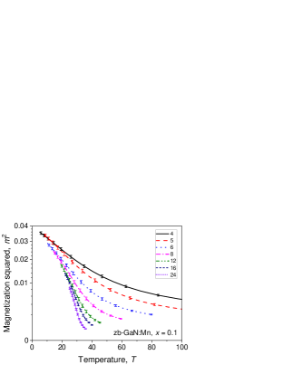
Figure 7: Examples of temperature dependence of magnetization square in zb-Ga_1-xMn_xN, $x=0.1$ obtained by the Monte-Carlo simulations.

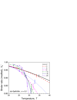
Figure 8: Examples of temperature dependencies of the modified Binder ratio for zb-Ga_1-xMn_xN, $x=0.1$ obtained by Monte-Carlo simulations.

It is interesting to compare the Monte-Carlo results to the expectations of the MFA and percolation theory for dilute ferromagnetic systems. For instance, in the case of zinc-blende Ga_0.9Mn_0.1N, according to Table 8 $T_{\text{C}}^{\text{MFA}}=124$ K, whereas $T_{\text{C}}^{\text{MC}}=28$ K. This significant difference was already noted in the context of ab initio studies of DFSs with short-range exchange interactions Sato et al. (2010).

The percolation theory Korenblit et al. (1973) was developed for continuous systems with exchange coupling $J(r)$ decaying exponentially with the spin pair distance $r$,

$$J(r)=J_{0}\exp\left(-r/b\right),$$ (18)

for which $T_{\text{C}}$ can be written in the form Korenblit et al. (1973),

$$T_{\text{C}}^{\text{perc}}\approx[S(2S+1)]J_{0}\exp\left(-\frac{0.89}{b\,(xN_{0})^{1/3}}\right),$$ (19)

where $N_{0}$ is the cation concentration of magnetic ions.

By fitting Eq. 18 to $J_{i}$ data displayed in Figs. 3, 5, and 6 we obtain, $J_{0}\approx 12.0,197,172\,\mathrm{K}$ and $b\approx 0.168,0.130$, and 0.136 nm for zb-(Zn,Cr)Te, zb-(Ga,Mn)N, and wz-(Ga,Mn)N, respectively. We omit fitting the data for (Hg,Cr)Te, as a departure from (18) is evident from oscillations of $J$. Similarly, we were unsuccessful fitting the alternative $J(r)$ for (Zn,Cr)Te (Fig. 4). As shown in Table 8, the resulting magnitudes of $T_{\text{C}}^{\text{perc}}$ agree with the $T_{\text{C}}$ values determined by Monte-Carlo simulations in both zb-(Ga,Mn)N and wz-(Ga,Mn)N. This agreement allows us to evaluate $T_{\text{C}}(x)$ from the percolation formula (19), avoiding computationally expensive Monte-Carlo simulations for many $x$ values and disorder realizations. In Fig. 9, the values of $T_{\text{C}}(x)$ we have obtained in this way are compared to experimental data Watanabe et al. (2019); Sarigiannidou et al. (2006); Sawicki et al. (2012); Stefanowicz et al. (2013) and earlier ab initio results Sato et al. (2010). As seen, the present theory predicts much smaller values of $T_{\text{C}}$ than the ab initio method which, within the local functional approximation, overestimates metallization of transition metal $d$ levels in semiconductors. Our $T_{\text{C}}$ values are lower than experimental points in the case of Zn_1-xCr_xTe at low $x$, which may point out to some aggregation of Cr ions in the studied layers, sensitivity to band-structure modelling, or significance of the departure from (18).

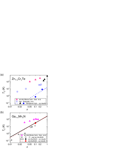
Figure 9: Curie temperatures $T_{\text{C}}$ in (a) Zn_1-xCr_xTe and (b) Ga_1-xMn_xN. Present results are shown by solid points obtained by tight-binding computations (Figs. 3–6) and Monte Carlo simulations. The fits of $J(r)$ served to determine $T_{\text{C}}(x)$ from the percolation theory, as shown by dotted and solid lines for zinc-blende and wurtzite systems, respectively. Solid triangles: alternative parameterization data (Fig. 4). Hollow triangles: previous ab initio and Monte Carlo results Sato et al. (2010); experimental data: squares Watanabe et al. (2019), diamond Sarigiannidou et al. (2006), stars Sawicki et al. (2012), circles Stefanowicz et al. (2013).

VI $sp$-$d$ exchange integrals and the quantum topological Hall effects

In tetrahedrally coordinated DMSs, exchange coupling between band carriers near the Brillouin zone center and cation-substitutional magnetic ions, ${\cal{H}}_{sp-d}^{(i)}=-{\cal{J}}\mathbf{s}\cdot\mathbf{S}_{i}$, is described by two exchange integrals Kacman (2001), $\alpha=\langle S|{\cal{J}}|S\rangle$ and $\beta=\langle X|{\cal{J}}|X\rangle$, where here $S$ and $X$ are the periodic part of the Bloch functions (Kohn-Luttinger amplitudes) that transform as atomic $s$ and $p_{x}$ wave functions under the point symmetry group operations. Typically, $\alpha$ and $\beta$ originate from the FM intra-atomic $s$-$d$ potential exchange and the $p$-$d$ hybridization, respectively. Furthermore, in many cases the molecular-field and virtual-crystal approximations hold allowing a straightforward determination of $\alpha$ and $\beta$ from band splittings once macroscopic magnetization is known.

Making use of NIST Atomic Spectra Database Levels, we obtain ${\cal{J}}_{\text{$4s$-$3d$}}=0.372$ eV for Cr¹⁺ ions, which constitutes an upper limit for the exchange energy $N_{0}\alpha$ in Cr-doped compounds. For comparison, ${\cal{J}}_{\text{$4s$-$3d$}}=0.391$ eV for Mn¹⁺, close to experimental Dobrowolska and Dobrowolski (1981); Bauer et al. (1985) and ab initio Autieri et al. (2021) values for (Hg,Mn)Te, $N_{0}\alpha=0.4\pm 0.1$ and $0.35\pm 0.05$ eV, respectively. In view of this discussion, we expect

$$N_{0}\alpha=0.3\pm 0.1\,\mathrm{eV}$$ (20)

for Hg_1-xCr_xTe.

However, in the case of wide-gap II-VI Mn-contained DMSs, in which the conduction-band wave function becomes significantly spread on anions, $N_{0}\alpha$ values are much reduced, e.g., $N_{0}\alpha=0.19$ eV in the case of (Zn,Mn)Te Twardowski et al. (1984). An interesting situation occurs in III-V DMS with Mn³⁺ ions, in which ferromagnetic $s$-$d$ coupling is compensated by antiferromagnetic exchange with holes tightly bound by Mn² ions Śliwa and Dietl (2008), resulting in $N_{0}\alpha=0.0\pm 0.1$ eV in wz-(Ga,Mn)N Suffczyński et al. (2011).

Using notation and parameter values introduced in Secs. II, the $p$-$d$ exchange energy for transition metal ions with the high-spin ($S=2$) $d^{4}$ configuration is given by Kacman (2001),

$$N_{0}\beta=V_{pd}^{2}\left(\frac{1}{3}\frac{1}{E_{d}}+\frac{2}{15}\frac{1}{E_{d}+U}-\frac{7}{15}\frac{1}{E_{d}+U+J}\right),$$ (21)

where ($P_{\mathrm{Te},p}$ projects the wavefunctions at $\Gamma$ onto the $p$-symmetry orbitals of tellurium)

$$V_{pd}=\frac{4}{3}\left(V_{pd\sigma}-\frac{2}{\sqrt{3}}V_{pd\pi}\right)\left|\left<\psi_{\Gamma}\middle|P_{\mathrm{Te},p}\middle|\psi_{\Gamma}\right>\right|,$$ (22)

which results in

$$N_{0}\beta=-1.8\pm 0.5\,\mathrm{eV}$$ (23)

for Hg_1-xCr_xTe in the small $x$ value limit and $E_{d}=-0.3\pm 0.1$ eV, with an about 50% enhancement in the alternative model which includes the $d$-$d$ hybridization. Large magnitudes of $N_{0}\alpha=0.3$ and $N_{0}\beta=-1.8$ eV mean that full polarization of Cr spins in Hg_0.99Cr_0.01Te will change $E_{g}$ by about 21 meV, strongly affecting optical and transport properties.

In the same way, we can evaluate a magnitude of the upward shift $\Delta E_{v}$ of the Hg_1-xCr_x valence band top in respect to HgTe, introduced by $p$-$d$ hybridization,

$$\Delta E_{v}=xN_{0}W_{pd}$$ (24)

$$= -xV_{pd}^{2}\left(\frac{1}{3}\frac{1}{E_{d}}+\frac{1}{5}\frac{1}{E_{d}+U}+\frac{7}{15}\frac{1}{E_{d}+U+J}\right).$$

This equation leads to

$$N_{0}W_{pd}=1.2\pm 0.5\,\mathrm{eV},$$ (25)

for Hg_1-xCr_xTe in the small $x$ limit. This value of $N_{0}W_{pd}$ implies that $p$-$d$ hybridization give a sizable contribution to the gap change. In particular, this fact is expected to enlarge the topological region, $E_{g}<0$, to $x\approx 10$% in Hg_1-xCr_xTe compare to Hg_1-xMn_xTe, where it extends to $x=7$%.

Particularly interesting is the case of Hg_1-xCr_xTe topological QWs. We assume that our evaluations of $\alpha$ and $\beta$ magnitudes are correct and list out expected phenomena brought about by cation-substitutional randomly distributed Cr ions. In the paramagnetic phase, guided by the Mn case Shamim et al. (2020), we expect that the range of QW thicknesses corresponding to the topological phase shrinks with $x$, and the trivial phase occurs at any thicknesses for $x\gtrsim 0.07$ Sawicki et al. (1983). In the topological phase, two new effects of paramagnetic impurities upon the quantum spin Hall effect have been recently identified Dietl (2023a, b):

1. The formation of bound magnetic polarons by holes residing on residual acceptor impurities. The associated spin-splitting $\Delta$ of acceptor states diminishes spin-flip Kondo backscattering of edge electrons by acceptor holes at low temperatures, $k_{B}T\lesssim\Delta(T)$, where $\Delta(T)$ scales with $\chi(T){\cal{J}}_{sp-d}^{2}$, where $\chi(T)$ is magnetic susceptibility of localized spins and ${\cal{J}}_{sp-d}^{2}$ is a weighted combination of $\alpha$ and $\beta$ Dietl (2023b). This model is experimentally corroborated by a recovery of the conductance quantization at low temperatures in topological Hg_1-xMn_xTe QWs Shamim et al. (2021).

2. Precessional dephasing of edge electron spins and momenta by a dense cloud of randomly oriented magnetic impurity spins. It has been argued that the constraint imposed by spin-momentum locking on the efficiency of backscattering by localized spins Tanaka et al. (2011) is relaxed by a flow of spin momenta to the bath of interacting magnetic impurities Dietl (2023b). This effect is relatively weakly dependent on temperature, as it scales with $T\chi(T){\cal{J}}_{sp-d}^{\prime 2}$, where ${\cal{J}}_{sp-d}^{\prime 2}$ is another combination of $\alpha$ and $\beta$ Dietl (2023b).

Interestingly, due to larger magnitudes of $\beta$ and $\chi$ (enhanced by ferromagnetic components in $J_{ij}$), both effects are expected to be substantially stronger in Hg_1-xCr_xTe compared to Hg_1-xMn_xTe.

Can one observe the anomalous quantum Hall effect in Hg_1-xCr_xTe quantum wells? As we noted, there is a competition of FM and AFM interactions, so that either FM or spin-glass phase is expected at low temperatures. Furthermore, it was demonstrated that the formation of a single chiral edge channels occurs for spin polarized magnetic ions along the growth direction, if $p=-\alpha/\beta\gtrsim 0.25$ Liu et al. (2008b), whereas the values quoted above point to $p=0.17\pm 0.1$. These two facts call for experimental verification. In the case of $p<0.25$, polarization of Cr spins, either spontaneous or driven by an external magnetic field along the growth direction, will lead to the closure of the topological gap and the associated colossal drop of resistance.

We note, however, that competition between spin-orbit and $p$-$d$ interactions makes that spin splitting of subbands with a heavy-hole character vanishes for the in-plane magnetization direction Peyla et al. (1993). This means that by tilting the magnetization direction one can change the parameter $p$. Figure 10 shows the subband structure for unstrained topological (Hg,Cr)Te/(Cd,Hg)Te QW in the absence of an external magnetic field, computed employing the eight bands’ $kp$ model in the axial approximation Novik et al. (2005); Dietl (2023b) with the values of $N_{0}\alpha$, $N_{0}\beta$, and $N_{0}W_{pd}$ quoted above. For (Hg,Cr)Te in a zinc-blende structure, as in any ferromagnetic cubic system, the magnetization easy axis assumes either the $\langle 100\rangle$ or $\langle 111\rangle$ crystallographic direction. As seen in Fig. 10, for the easy axis along the growth direction, $\mathbf{M}\|[001]$, the presence of non-zero magnetization tends to close the gap, in agreement with the value $p<0.25$. In contrast, for $\mathbf{M}\|\langle 111\rangle$, the topological gap persists and, moreover, the inverted band structure is present for the spin-down channel only. We conclude that the quantum anomalous Hall effect is expected under these conditions.

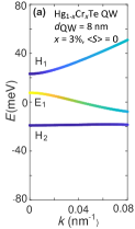
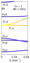
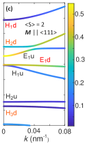
Figure 10: Computed subband structure in unstrained Hg_0.97Cr_0.03Te/(Cd,Hg)Te quantum wells; labels H and E refer to subbands originating from the heavy-hole and electron-like bands in non-topological semiconductors; d and u correspond to spin-down and spin-up subbands. (a) Paramagnetic case, i.e. average Cr spin $\langle S\rangle=0$; (b) $\langle S\rangle=2$ and magnetization is oriented along the growth direction; (c) $\langle S\rangle=2$ and magnetization is oriented along one of $\langle 111\rangle$ directions. Colors describe the participation of the $s_{1/2,\pm 1/2}$ Kohn-Luttinger amplitude in the electronic wave function; Hg_0.97Cr_0.03Te QW thickness $d_{\text{QW}}=8$ nm.

Finally, we mention that in the case of (Zn,Cr)Te and (Ga,Mn)N the relevant donor level introduced by TM ions resides in the gap, i.e., $E_{d}>0$. In qualitative agreement with Eq. 21, the FM sign of $\beta$ was observed in these two systems Twardowski et al. (1987); Suffczyński et al. (2011). However, as mentioned when discussing $N_{0}\alpha$ case, the Mn³ state can be regarded as the Mn²⁺ acceptor with a tightly bound hole. The resulting bare coupling between a band hole and Mn²⁺ ion is then AFM. However, the experimentally proven existence of the hole bound state in the gap (Mn^3+/4+ complex with $E_{d}=1.1$ eV) means that band hole can be trapped by Mn, meaning that the molecular-field approximation does not hold. A non-perturbative approach demonstrates that the apparent $p$-$d$ coupling is FM under these conditions Dietl (2008), in agreement with experimental findings Suffczyński et al. (2011).

VII Conclusions and outlook

We have presented the theoretical results for $d$-$d$ and $p$-$d$ exchange interactions in diluted magnetic insulators for the $S=2$ case, i.e., for Cr in HgTe and ZnTe as well as for Mn in zinc-blende and wurtzite GaN. Our approach not only addresses some weak points of earlier theories of ferromagnetic superexchange but takes into account the interband Bloenbergen-Rowland-Van Vleck and two-electron contributions. These additional terms are of a lesser importance in (Ga,Mn)N but play a significant role in (Zn,Cr)Te and, particularly, in topological (Hg,Cr)Te, where they introduce antiferromagnetic coupling for certain pairs of Cr atoms. We have found that the presence of the competing interactions makes that the theoretical results become rather sensitive to the adopted tight-binding model of the host band structure. Because of this competition, and in agreement with experimental data, Curie temperatures $T_{\text{C}}$ in (Zn,Cr)Te are expected to be lower compared to (Ga,Mn)N with the identical concentration of magnetic ions. At the same time, we cannot exclude the presence of a spin-glass phase rather than ferromagnetism in topological (Hg,Cr)Te. If this would be the case, a relatively large magnitude of the $p$-$d$ exchange integral $\beta$ that we predict for (Hg,Cr)Te should stabilize the quantum spin Hall effect by the formation of bound magnetic polarons that weaken Kondo backscattering of edge electrons by holes trapped to residual acceptor impurities. The large magnitude of $\beta$ means also that the quantum anomalous Hall effect can be observed in topological (Hg,Cr)Te for the magnetization vector tilted away from the direction perpendicular to the quantum well plane.

Compared to ferromagnetic Bi-Sb chalcogenides, it is harder to introduce Cr and V to HgTe and related systems. However, once obtained, they should show lower areal density of native defects, as according to gating characteristics, the concentration of the in-gap localized states is almost two orders of magnitude smaller in HgTe quantum wells Bendias et al. (2018); Yahniuk et al. than in (Bi,Sb,Cr,V)₂Te₃ layers Okazaki et al. (2022); Fijalkowski et al. (2021); Rodenbach et al. (2023). As the exchange gap is typically in the tens meV range (see Fig. 10), we assign the thermally activated conductivity $\sigma_{xx}$ in (Bi,Sb,Cr,V)₂Te₃ layers Okazaki et al. (2022); Fijalkowski et al. (2021); Rodenbach et al. (2023) to the Efros-Shklovskii hopping between in-gap states. A lower concentration of such states will allow for the operation of resistance standards at higher temperature.

Appendix A Transformation matrix to $T_{2}\oplus E$

With the threefold wurtzite $c$-axis as the $z$ (quantization) axis, a symmetry-invariant decomposition of the Hilbert space for $L=2$ into $3+2$ dimensions ($T_{2}\oplus E$) is parameterized below by $(\theta,\phi)$ [cf. Eq. 68 of Ref. Goodenough, 1963]. The threefold symmetry acts by cycling the $T_{2}$ vectors $(\psi_{T_{2},i})_{i=1,2,3}$. Under cubic symmetry, $\cos(\theta)=1/\sqrt{3}$; the deviation from this value is a material parameter. On the other hand, due to the wurtzite mirror symmetry, $\phi$ is not variable, but it takes different and conventions-dependent values for the two inequivalent cation positions Yang et al. (1995) (here, $\phi=-\pi/2$ for $t_{2}$ and $\phi=\pi/2$ for $t_{4}$).

$$\left<yz\middle|\psi_{T_{2},1}\right> = \sqrt{2/3}\cos(\theta)\sin(\phi)$$ (26)

$$\left<xz\middle|\psi_{T_{2},1}\right> = -\sqrt{2/3}\cos(\theta)\cos(\phi)$$ (27)

$$\left<xy\middle|\psi_{T_{2},1}\right> = -\sqrt{2/3}\sin(\theta)\sin(2\phi)$$ (28)

$$\left<3z^{2}-r^{2}\middle|\psi_{T_{2},1}\right> = \sqrt{1/3}$$ (29)

$$\left<x^{2}-y^{2}\middle|\psi_{T_{2},1}\right> = \sqrt{2/3}\sin(\theta)\cos(2\phi)$$ (30)

$$\left<yz\middle|\psi_{T_{2},2}\right> = -\cos\theta\left[3\cos(\phi)+\sqrt{3}\sin(\phi)\right]/(3\sqrt{2})$$ (31)

$$\left<xz\middle|\psi_{T_{2},2}\right> = \cos\theta\left[\cos(\phi)/\sqrt{6}-\sin(\phi)/\sqrt{2}\right]$$ (32)

$$\left<xy\middle|\psi_{T_{2},2}\right> = -\sin\theta\left[\cos(2\phi)/\sqrt{2}-\sin(2\phi)/\sqrt{6}\right]$$ (33)

$$\left<3z^{2}-r^{2}\middle|\psi_{T_{2},2}\right> = \sqrt{1/3}$$ (34)

$$\left<x^{2}-y^{2}\middle|\psi_{T_{2},2}\right> = -\sin\theta\left[\sqrt{3}\cos(2\phi)+3\sin(2\phi)\right]/(3\sqrt{2})$$ (35)

$$\left<yz\middle|\psi_{T_{2},3}\right> = \cos\theta\left[\cos(\phi)/\sqrt{2}-\sin(\phi)/\sqrt{6}\right]$$ (36)

$$\left<xz\middle|\psi_{T_{2},3}\right> = \cos\theta\left[\cos(\phi)/\sqrt{6}+\sin(\phi)/\sqrt{2}\right]$$ (37)

$$\left<xy\middle|\psi_{T_{2},3}\right> = \sin\theta\left[\cos(2\phi)/\sqrt{2}+\sin(2\phi)/\sqrt{6}\right]$$ (38)

$$\left<3z^{2}-r^{2}\middle|\psi_{T_{2},3}\right> = \sqrt{1/3}$$ (39)

$$\left<x^{2}-y^{2}\middle|\psi_{T_{2},3}\right> = -\sin\theta\left[\cos(2\phi)/\sqrt{6}-\sin(2\phi)/\sqrt{2}\right]$$ (40)

$$\left<yz\middle|\psi_{E,1}\right> = -\sin\theta\left[\cos(\phi)+\sin(\phi)\right]/\sqrt{2}$$ (41)

$$\left<xz\middle|\psi_{E,1}\right> = \sin\theta\left[\cos(\phi)/\sqrt{6}+\sin(\phi)/\sqrt{2}\right]$$ (42)

$$\left<xy\middle|\psi_{E,1}\right> = \cos\theta\left[\cos(\phi)-\sin(\phi)\right]/\sqrt{2}$$ (43)

$$\left<3z^{2}-r^{2}\middle|\psi_{E,1}\right> = 0$$ (44)

$$\left<x^{2}-y^{2}\middle|\psi_{E,1}\right> = \cos\theta\left[\cos(2\phi)+\sin(2\phi)\right]/\sqrt{2}$$ (45)

$$\left<yz\middle|\psi_{E,2}\right> = \sin\theta\left[\cos(\phi)-\sin(\phi)\right]/\sqrt{2}$$ (46)

$$\left<xz\middle|\psi_{E,2}\right> = \sin\theta\left[\cos(\phi)+\sin(\phi)\right]/\sqrt{2}$$ (47)

$$\left<xy\middle|\psi_{E,2}\right> = -\cos\theta\left[\cos(2\phi)+\sin(2\phi)\right]/\sqrt{2}$$ (48)

$$\left<3z^{2}-r^{2}\middle|\psi_{E,2}\right> = 0$$ (49)

$$\left<x^{2}-y^{2}\middle|\psi_{E,2}\right> = \cos\theta\left[\cos(2\phi)-\sin(2\phi)\right]/\sqrt{2}$$ (50)

Appendix B Definitions of the correlation lengths

The definition of the correlation length varies from a crystal structure to another. For wurtzite, we assume that the correlator decays exponentially with distance ($\mathbf{r}=x_{1}\mathbf{a}_{1}+x_{2}\mathbf{a}_{2}+x_{3}\mathbf{a}_{3}$) as:

$$C(\mathbf{r})=\exp\left(-\frac{(|x_{1}|+|x_{2}|+|x_{1}+x_{2}|)}{\xi_{a}}\right)\exp\left(-\frac{|x_{3}|}{\xi_{c}}\right).$$ (51)

We estimate $\xi_{c}$ as follows: a simulation is performed in a lattice block of size $L_{1}\times L_{2}\times L_{3}$, $L_{1}/L_{3}=L_{2}/L_{3}=3/2$, and the susceptibility $\chi_{k=k_{min,c}}$ at momentum $k_{min,c}=(k_{1},k_{2},k_{3})=\left(0,0,\frac{4\pi}{L_{3}}\right)$, together with magnetization squared (i.e. the susceptibility at zero momentum, $k_{1}=k_{2}=k_{3}=0$), are both evaluated. We define $\xi_{wz,c}\approx\xi_{c}$ as

$$\xi_{wz,c}\approx\frac{1}{3\sin{\frac{4\pi}{3L_{3}}}}\sqrt{\frac{\chi_{k=0}}{\chi_{k=k_{min,c}}}-1}.$$ (52)

Analogously, $\xi_{wz,a}\approx\xi_{a}$ can be defined as

$$\xi_{wz,a}\approx\frac{7}{18\sin{\frac{2\pi}{L_{1}}}}\sqrt{\frac{\chi_{k=0}}{\chi_{k=k_{min,a}}}-1},$$ (53)

with $k_{min,a}=\left(\frac{6\pi}{L_{1}},0,0\right)$.

References

- Dietl and Ohno (2014) T. Dietl and H. Ohno, “Dilute ferromagnetic semiconductors: Physics and spintronic structures,” Rev. Mod. Phys. 86, 187–251 (2014).
- Jungwirth et al. (2014) T. Jungwirth, J. Wunderlich, V. Novák, K. Olejník, B. L. Gallagher, R. P. Campion, K. W. Edmonds, A. W. Rushforth, A. J. Ferguson, and P. Němec, “Spin-dependent phenomena and device concepts explored in (Ga,Mn)As,” Rev. Mod. Phys. 86, 855–896 (2014).
- Sztenkiel et al. (2016) D. Sztenkiel, M. Foltyn, G. P. Mazur, R. Adhikari, K. Kosiel, K. Gas, M. Zgirski, R. Kruszka, R. Jakieła, Tian Li, A. Piotrowska, A. Bonanni, M. Sawicki, and T. Dietl, “Stretching magnetism with an electric field in a nitride semiconductor,” Nat. Commun. 7, 13232 (2016).
- Mogi et al. (2022) M. Mogi, Y. Okamura, M. Kawamura, R. Yoshimi, K. Yasuda, A. Tsukazaki, K. S. Takahashi, T. Morimoto, N. Nagaosa, M. Kawasaki, Y. Takahashi, and Y. Tokura, “Experimental signature of the parity anomaly in a semi-magnetic topological insulator,” Nat. Phys. 18, 390–394 (2022).
- Yu et al. (2010) Rui Yu, Wei Zhang, Hai-Jun Zhang, Shou-Cheng Zhang, Xi Dai, and Zhong Fang, “Quantized anomalous Hall effect in magnetic topological insulators,” Science 329, 61–64 (2010).
- Chang et al. (2013) Cui-Zu Chang, Jinsong Zhang, Xiao Feng, Jie Shen, Zuocheng Zhang, Minghua Guo, Kang Li, Yunbo Ou, Pang Wei, Li-Li Wang, Zhong-Qing Ji, Yang Feng, Shuaihua Ji, Xi Chen, Jinfeng Jia, Xi Dai, Zhong Fang, Shou-Cheng Zhang, Ke He, Yayu Wang, Li Lu, Xu-Cun Ma, and Qi-Kun Xue, “Experimental observation of the quantum anomalous Hall effect in a magnetic topological insulator,” Science 340, 167–170 (2013).
- Ke et al. (2018) He Ke, Yayu Wang, and Qi-Kun Xue, “Topological materials: quantum anomalous Hall system,” Annu. Rev. Cond. Mat. Phys. 9, 329–344 (2018).
- Tokura et al. (2019) Y. Tokura, K. Yasuda, and A. Tsukazaki, “Magnetic topological insulators,” Nat. Rev. Phys. 1, 126–143 (2019).
- Bernevig et al. (2022) B. A. Bernevig, C. Felser, and H. Beidenkopf, “Progress and prospects in magnetic topological materials,” Nature 603, 41–51 (2022).
- Chang et al. (2023) Cui-Zu Chang, Chao-Xing Liu, and A. H. MacDonald, “Quantum anomalous Hall effect,” Rev. Mod. Phys. 95, 011002 (2023).
- Goetz et al. (2018) M. Goetz, K. M. Fijalkowski, E. Pesel, M. Hartl, S. Schreyeck, M. Winnerlein, S. Grauer, H. Scherer, K. Brunner, C. Gould, F. J. Ahlers, and L. W. Molenkamp, “Precision measurement of the quantized anomalous Hall resistance at zero magnetic field,” Appl. Phys. Lett. 112, 072102 (2018).
- Fox et al. (2018) E. J. Fox, I. T. Rosen, Yanfei Yang, G. R. Jones, R. E. Elmquist, Xufeng Kou, Lei Pan, Kang L. Wang, and D. Goldhaber-Gordon, “Part-per-million quantization and current-induced breakdown of the quantum anomalous Hall effect,” Phys. Rev. B 98, 075145 (2018).
- Okazaki et al. (2022) Y. Okazaki, T. Oe, M. Kawamura, R. Yoshimi, S. Nakamura, S. Takada, M. Mogi, K. S. Takahashi, A. Tsukazaki, M. Kawasaki, Y. Tokura, and N.-H. Kaneko, “Quantum anomalous Hall effect with a permanent magnet defines a quantum resistance standard,” Nat. Phys. 18, 25 (2022).
- Rodenbach et al. (2023) L. K. Rodenbach, Ngoc Thanh Mai Tran, J. M. Underwood, A. R. Panna, M. P. Andersen, Z. S. Barcikowski, S. U. Payagala, Peng Zhang, Lixuan Tai, Kang L. Wang, R. E. Elmquist, D. G. Jarrett, D. B. Newell, A. F. Rigosi, and D. Goldhaber-Gordon, “Realization of the quantum ampere using the quantum anomalous Hall and Josephson effects,” arXiv:2308.00200 (2023), 10.48550/arXiv.2308.00200.
- Peixoto et al. (2020) T. R. F. Peixoto, H. Bentmann, P. Rüßmann, A.-V. Tcakaev, M. Winnerlein, S. Schreyeck, S. Schatz, R. C. Vidal, F. Stier, V. Zabolotnyy, R. J. Green, Chul Hee Min, C. I. Fornari, Maaß H., H. B. Vasili, P. Gargiani, M. Valvidares, A. Barla, J. Buck, M. Hoesch, F. Diekmann, S. Rohlf, M. Kalläne, K. Rossnagel, Ch. Gould, K. Brunner, S. Blügel, V. Hinkov, L. W. Molenkamp, and F. Reinert, “Non-local effect of impurity states on the exchange coupling mechanism in magnetic topological insulators,” npj Quant. Mater. 5, 87 (2020).
- Śliwa et al. (2021) C. Śliwa, C. Autieri, J. A. Majewski, and T. Dietl, “Superexchange dominates in magnetic topological insulators,” Phys. Rev. B 104, L220404 (2021).
- Watanabe et al. (2019) R. Watanabe, R. Yoshimi, M. Kawamura, M. Mogi, A. Tsukazaki, X. Z. Yu, K. Nakajima, K. S. Takahashi, M. Kawasaki, and Y. Tokura, “Quantum anomalous Hall effect driven by magnetic proximity coupling in all-telluride based heterostructure,” Appl. Phys. Lett. 115, 102403 (2019).
- Escribano et al. (2022) S. D. Escribano, A. Maiani, M. Leijnse, K. Flensberg, Y. Oreg, A. Levy Yeyati, E. Prada, and R. Seoane Souto, “Semiconductor-ferromagnet-superconductor planar heterostructures for 1D topological superconductivity,” npj Quant. Mater. 7, 81 (2022).
- Goodenough (1963) John B. Goodenough, Magnetism and the Chemical Bond, Interscience Monographs on Chemistry (Interscience Publishers, 1963).
- Blinowski et al. (1996) J. Blinowski, P. Kacman, and J. A. Majewski, “Ferromagnetic superexchange in Cr-based diluted magnetic semiconductors,” Phys. Rev. B 53, 9524–9527 (1996).
- Kuroda et al. (2007a) S. Kuroda, N. Nishizawa, K. Takita, M. Mitome, Y. Bando, K. Osuch, and T. Dietl, “Origin and control of high-temperature ferromagnetism in semiconductors,” Nat. Mater. 6, 440 (2007a).
- Sarigiannidou et al. (2006) E. Sarigiannidou, F. Wilhelm, E. Monroy, R. M. Galera, E. Bellet-Amalric, A. Rogalev, J. Goulon, J. Cibert, and H. Mariette, “Intrinsic ferromagnetism in wurtzite (Ga,Mn)N semiconductor,” Phys. Rev. B 74, 041306 (2006).
- Sawicki et al. (2012) M. Sawicki, T. Devillers, S. Gałęski, C. Simserides, S. Dobkowska, B. Faina, A. Grois, A. Navarro-Quezada, K. N. Trohidou, J. A. Majewski, T. Dietl, and A. Bonanni, “Origin of low-temperature magnetic ordering in ,” Phys. Rev. B 85, 205204 (2012).
- Stefanowicz et al. (2013) S. Stefanowicz, G. Kunert, C. Simserides, J. A. Majewski, W. Stefanowicz, C. Kruse, S. Figge, Tian Li, R. Jakieła, K. N. Trohidou, A. Bonanni, D. Hommel, M. Sawicki, and T. Dietl, “Phase diagram and critical behavior of the random ferromagnet ,” Phys. Rev. B 88, 081201(R) (2013).
- Simserides et al. (2014) C. Simserides, J.A. Majewski, K.N. Trohidou, and T. Dietl, “Theory of ferromagnetism driven by superexchange in dilute magnetic semiconductors,” EPJ Web of Conferences 75, 01003 (2014).
- Bloembergen and Rowland (1955) N. Bloembergen and T. J. Rowland, “Nuclear spin exchange in solids: and magnetic resonance in thallium and thallic oxide,” Phys. Rev. 97, 1679–1698 (1955).
- Lewiner et al. (1980) C. Lewiner, J. Gaj, and G. Bastard, “Indirect exchange interaction in and alloys,” J. Phys. Colloq. (Paris) 41 (C5), 289–292 (1980).
- Larson et al. (1988) B. E. Larson, K. C. Hass, H. Ehrenreich, and A. E. Carlsson, “Theory of exchange interactions and chemical trends in diluted magnetic semiconductors,” Phys. Rev. B 37, 4137–4154 (1988).
- Dietl et al. (2001) T. Dietl, H. Ohno, and F. Matsukura, “Hole-mediated ferromagnetism in tetrahedrally coordinated semiconductors,” Phys. Rev. B 63, 195205 (2001).
- Kacman (2001) P. Kacman, “Spin interactions in diluted magnetic semiconductors and magnetic semiconductor structures,” Semicon. Sci. Technol. 16, R25–R39 (2001).
- Śliwa and Dietl (2018) C. Śliwa and T. Dietl, “Thermodynamic perturbation theory for noninteracting quantum particles with application to spin-spin interactions in solids,” Phys. Rev. B 98, 035105 (2018).
- Korenblit et al. (1973) I. Ya. Korenblit, E. F. Shender, and B. I. Shklovsky, “Percolation approach to the phase transition in very dilute ferromagnetic alloys,” Phys. Lett. A 46, 275–276 (1973).
- Sato et al. (2010) K. Sato, L. Bergqvist, J. Kudrnovský, P. H. Dederichs, O. Eriksson, I. Turek, B. Sanyal, G. Bouzerar, H. Katayama-Yoshida, V. A. Dinh, T. Fukushima, H. Kizaki, and R. Zeller, “First-principles theory of dilute magnetic semiconductors,” Rev. Mod. Phys. 82, 1633–1690 (2010).
- Bonanni et al. (2021) A. Bonanni, T. Dietl, and H. Ohno, “Dilute magnetic materials,” in Handbook of Magnetism and Magnetic Materials, edited by M. Coey and S. Parkin (Springer, Berlin, 2021).
- Dietl (2008) T. Dietl, “Hole states in wide band-gap diluted magnetic semiconductors and oxides,” Phys. Rev. B 77, 085208 (2008).
- Mac et al. (1996) W. Mac, A. Twardowski, and M. Demianiuk, “s,p-d exchange interaction in Cr-based diluted magnetic semiconductors,” Phys. Rev. B 54, 5528–5535 (1996).
- Suffczyński et al. (2011) J. Suffczyński, A. Grois, W. Pacuski, A. Golnik, J. A. Gaj, A. Navarro-Quezada, B. Faina, T. Devillers, and A. Bonanni, “Effects of ,- and - exchange interactions probed by exciton magnetospectroscopy in (Ga,Mn)N,” Phys. Rev. B 83, 094421 (2011).
- Liu et al. (2008a) Chao-Xing Liu, Xiao-Liang Qi, Xi Dai, Zhong Fang, and Shou-Cheng Zhang, “Quantum Anomalous Hall Effect in Quantum Wells,” Phys. Rev. Lett. 101, 146802 (2008a).
- Kuroda et al. (2007b) S. Kuroda, N. Nishizawa, K. Takita, M. Mitome, Y. Bando, K. Osuch, and T. Dietl, “Origin and control of high-temperature ferromagnetism in semiconductors,” Nat. Mater. 6, 440–446 (2007b).
- Graf et al. (2003) Tobias Graf, Sebastian T. B. Goennenwein, and Martin S. Brandt, “Prospects for carrier-mediated ferromagnetism in GaN,” physica status solidi (b) 239, 277–290 (2003).
- Han et al. (2005) B. Han, B. W. Wessels, and M. P. Ulmer, “Optical investigation of electronic states of ions in -type GaN,” Appl. Phys. Lett. 86, 042505 (2005).
- Hwang et al. (2005) J. I. Hwang, Y. Ishida, M. Kobayashi, H. Hirata, K. Takubo, T. Mizokawa, A. Fujimori, J. Okamoto, K. Mamiya, Y. Saito, Y. Muramatsu, H. Ott, A. Tanaka, T. Kondo, and H. Munekata, “High-energy spectroscopic study of the III–V nitride-based diluted magnetic semiconductor ,” Phys. Rev. B 72, 085216 (2005).
- Bertho et al. (1991) D. Bertho, D. Boiron, A. Simon, C. Jouanin, and C. Priester, “Calculation of hydrostatic and uniaxial deformation potentials with a self-consistent tight-binding model for Zn-cation-based II-VI compounds,” Phys. Rev. B 44, 6118–6124 (1991).
- Shi and Papaconstantopoulos (2004) Lei Shi and Dimitrios A. Papaconstantopoulos, “Modifications and extensions to Harrison’s tight-binding theory,” Phys. Rev. B 70, 205101 (2004).
- Parmenter (1973) R. H. Parmenter, “Effect of orbital degeneracy on the Anderson model of a localized moment in a metal,” Phys. Rev. B 8, 1273–1275 (1973).
- Winkler (2003) Roland Winkler, Spin-orbit coupling effects in two-dimensional electron and hole systems (Springer Verlag, Berlin, Heidelberg, 2003).
- Allan and Delerue (2012) Guy Allan and Christophe Delerue, “Tight-binding calculations of the optical properties of HgTe nanocrystals,” Phys. Rev. B 86, 165437 (2012).
- Sapra et al. (2002) Sameer Sapra, N. Shanthi, and D. D. Sarma, “Realistic tight-binding model for the electronic structure of II-VI semiconductors,” Phys. Rev. B 66, 205202 (2002).
- Spałek et al. (1986) J. Spałek, A. Lewicki, Z. Tarnawski, J. K. Furdyna, R. R. Galazka, and Z. Obuszko, “Magnetic susceptibility of semimagnetic semiconductors: The high-temperature regime and the role of superexchange,” Phys. Rev. B 33, 3407–3418 (1986).
- Bonanni et al. (2011) A. Bonanni, M. Sawicki, T. Devillers, W. Stefanowicz, B. Faina, Tian Li, T. E. Winkler, D. Sztenkiel, A. Navarro-Quezada, M. Rovezzi, R. Jakieła, A. Grois, M. Wegscheider, W. Jantsch, J. Suffczyński, F. D’Acapito, A. Meingast, G. Kothleitner, and T. Dietl, “Experimental probing of exchange interactions between localized spins in the dilute magnetic insulator (Ga,Mn)N,” Phys. Rev. B 84, 035206 (2011).
- Śliwa (2022) C. Śliwa, “Disorder-averaged Binder ratio in site-diluted Heisenberg model,” (2022), arXiv:2205.00977.
- Dobrowolska and Dobrowolski (1981) M. Dobrowolska and W. Dobrowolski, “Temperature study of interband magnetoabsorption in mixed crystals,” J. Phys. C: Solid State Phys. 14, 5689 (1981).
- Bauer et al. (1985) G. Bauer, J. Kossut, R. Faymonville, and R. Dornhaus, “Magnetoreflectivity study of the band structure of Te (0.026x0.106),” Phys. Rev. B 31, 2040–2048 (1985).
- Autieri et al. (2021) C. Autieri, C. Śliwa, R. Islam, G. Cuono, and T. Dietl, “Momentum-resolved spin splitting in Mn-doped trivial CdTe and topological HgTe semiconductors,” Phys. Rev. B 103, 115209 (2021).
- Twardowski et al. (1984) A. Twardowski, P. Swiderski, M. von Ortenberg, and R. Pauthenet, “Magnetoabsorption and magnetization of Zn1-xMnxTe mixed crystals,” Solid State Commun. 50, 509–513 (1984).
- Śliwa and Dietl (2008) Cezary Śliwa and Tomasz Dietl, “Electron-hole contribution to the apparent exchange interaction in III-V dilute magnetic semiconductors,” Phys. Rev. B 78, 165205 (2008).
- Shamim et al. (2020) S. Shamim, W. Beugeling, J. Böttcher, P. Shekhar, A. Budewitz, P. Leubner, L. Lunczer, E. M. Hankiewicz, H. Buhmann, and L. W. Molenkamp, “Emergent quantum Hall effects below 50 mT in a two-dimensional topological insulator,” Adv. Sci. 6, eaba4625 (2020).
- Sawicki et al. (1983) M. Sawicki, T. Dietl, W. Plesiewicz, P. Sękowski, L. Śniadower, M. Baj, and L. Dmowski, “Influence of an acceptor state on transport in zero-gap Hg1-xMnxTe,” in Application of High Magnetic Fields in Semiconductor Physics, edited by G. Landwehr (Springer Berlin Heidelberg, Berlin, Heidelberg, 1983) pp. 382–385.
- Dietl (2023a) T. Dietl, “Effects of charge dopants in quantum spin Hall materials,” Phys. Rev. Lett. 130, 086202 (2023a).
- Dietl (2023b) T. Dietl, “Quantitative theory of backscattering in topological HgTe and (Hg,Mn)Te quantum wells: Acceptor states, Kondo effect, precessional dephasing, and bound magnetic polaron,” Phys. Rev. B 107, 085421 (2023b).
- Shamim et al. (2021) S. Shamim, W. Beugeling, P. Shekhar, K. Bendias, L. Lunczer, J. Kleinlein, H. Buhmann, and L. W. Molenkamp, “Quantized spin Hall conductance in a magnetically doped two dimensional topological insulator,” Nat. Commun. 12, 3193 (2021).
- Tanaka et al. (2011) Y. Tanaka, A. Furusaki, and K. A. Matveev, “Conductance of a helical edge liquid coupled to a magnetic impurity,” Phys. Rev. Lett. 106, 236402 (2011).
- Liu et al. (2008b) Chao-Xing Liu, Xiao-Liang Qi, Xi Dai, Zhong Fang, and Shou-Cheng Zhang, “Quantum anomalous Hall effect in Hg1-yMnyTe quantum wells,” Phys. Rev. Lett. 101, 146802 (2008b).
- Peyla et al. (1993) P. Peyla, A. Wasiela, Y. Merle d’Aubigné, D. E. Ashenford, and B. Lunn, “Anisotropy of the zeeman effect in CdTe/Te multiple quantum wells,” Phys. Rev. B 47, 3783–3789 (1993).
- Novik et al. (2005) E. G. Novik, A. Pfeuffer-Jeschke, T. Jungwirth, V. Latussek, C. R. Becker, G. Landwehr, H. Buhmann, and L. W. Molenkamp, “Band structure of semimagnetic Hg1-yMnyTe quantum wells,” Phys. Rev. B 72, 035321 (2005).
- Twardowski et al. (1987) A. Twardowski, H. J. M. Swagten, W. J. M. de Jonge, and M. Demianiuk, “Magnetic behavior of the diluted magnetic semiconductor Se,” Phys. Rev. B 36, 7013–7023 (1987).
- Bendias et al. (2018) K. Bendias, S. Shamim, O. Herrmann, A. Budewitz, P. Shekhar, P. Leubner, J. Kleinlein, E. Bocquillon, H. Buhmann, and L. W. Molenkamp, “High mobility HgTe microstructures for quantum spin Hall studies,” Nano Lett. 18, 4831–4836 (2018).
- (68) I. Yahniuk, A. Kazakov, B. Jouault, S. S. Krishtopenko, S. Kret, G. Grabecki, G. Cywiński, N. N. Mikhailov, S. A. Dvoretskii, J. Przybytek, V. I. Gavrilenko, F. Teppe, T. Dietl, and W. Knap, “HgTe quantum wells for QHE metrology under soft cryomagnetic conditions: permanent magnets and liquid 4He temperatures,” 10.48550/arXiv.2111.07581.
- Fijalkowski et al. (2021) K. M. Fijalkowski, Nan Liu, P. Mandal, S. Schreyeck, K. Brunner, C. Gould, and L. W. Molenkamp, “Quantum anomalous Hall edge channels survive up to the Curie temperature,” Nat. Commun. 12, 5599 (2021).
- Yang et al. (1995) Tao Yang, Sadanojo Nakajima, and Shiro Sakai, “Electronic structures of wurtzite GaN, InN and their alloy calculated by the tight-binding method,” Jpn. J. Appl. Phys. 34, 5912 (1995).