Soft modes in hot QCD matter

Abstract

The chiral crossover of QCD at finite temperature and vanishing baryon density turns into a second order phase transition if lighter than physical quark masses are considered. If this transition occurs sufficiently close to the physical point, its universal critical behaviour would largely control the physics of the QCD phase transition. We quantify the size of this region in QCD using functional approaches, both Dyson-Schwinger equations and the functional renormalisation group. The latter allows us to study both critical and non-critical effects on an equal footing, facilitating a precise determination of the scaling regime. We find that the physical point is far away from the critical region. Importantly, we show that the physics of the chiral crossover is dominated by soft modes even far beyond the critical region. While scaling functions determine all thermodynamic properties of the system in the critical region, the order parameter potential is the relevant quantity away from it. We compute this potential in QCD using the functional renormalisation group and Dyson-Schwinger equations and provide a simple parametrisation for phenomenological applications.

Introduction.– It has been argued that physical QCD at vanishing chemical potential could be in the critical scaling region of the chiral phase transition around the limit of massless quarks [1, 2, 3, 4, 5, 6]. These studies have to be contrasted with analyses of QCD based on the functional renormalisation group (fRG) [7, 8] that indicate a very small scaling region. The answer to this question is of phenomenological relevance as light low-momentum modes, so-called soft modes, dominate the dynamical evolution of the system created in a heavy-ion collision. If these modes exhibit critical scaling even at high beam energies, their contribution is well described by the respective universal critical dynamics, e.g., [9, 10, 11, 12, 13].

In the critical region, physical quantities such as the order parameter $\Delta$ are dominated by scaling behaviour, e.g., $\Delta(H)\sim H^{\frac{1}{\delta}}$, where $\delta$ is a universal critical exponent and $H$ an external field, see, e.g., [14]. For the chiral phase transition in QCD, $H$ can be identified with the light current quark mass. Crucially, this behaviour persists over many orders of magnitude in $H$. This poses the challenge both for theory and experiment that $\Delta(H)$ has to be known with high precision over a wide range of quark masses in order to make conclusive statements about universality. Furthermore, universality can only be used in the regime with negligible non-critical contributions. As demonstrated in [15], conclusions about critical behaviour drawn from a scaling analysis may otherwise be incorrect. Therefore, it is clear that an analysis of the chiral critical behaviour with currently available lattice data [1, 2, 3, 4, 5, 6] requires great care.

In the present work we report on a conclusive scaling analysis with pion masses ranging over five orders of magnitude and as small as $m_{\pi}=0.002\,\text{MeV}$. This allows us to determine the size of the critical region of the chiral phase transition in QCD around the chiral limit. A key advantage of our renormalisation group based analysis is that fixed points are straightforwardly identified and the corresponding critical exponents can systematically be extracted with high precision within a given approximation [16, 17, 18, 19]. This facilitates the precise determination of the scaling region of the chiral phase transition of QCD.

The relevance of the magnetic equation of state $\Delta(H)$ and, more precisely that of the order parameter potential persists beyond the critical region. These quantities describe the universal and non-universal behaviour of the system and are the crucial input for the phenomenological modelling of heavy-ion collisions. In the present work, we provide these quantities using functional approaches to QCD, i.e., the fRG approach and Dyson-Schwinger equations (DSE). We compute these quantities over many orders of magnitude in $H$ around and in particular below the physical point. The reliability of our results is corroborated by the excellent agreement of fRG and DSE results. We evaluate where soft modes dominate hot QCD matter and argue that their presence is the phenomenologically relevant property. Chiral criticality is only a very small aspect of this property and we will demonstrate that it is irrelevant for QCD at the physical point.

Magnetic equation of state and the critical region.– The magnetic equation of state governs the $(T,m_{q})$-dependence of the chiral condensate

$$\Delta_{q}(m_{q}\big{)}=m_{q}\frac{\partial\Omega\big{(}m_{q}\big{)}}{\partial m_{q}}=m_{q}\frac{T}{V}\int_{x}\!\big{\langle}\bar{q}(x)\,q(x)\big{\rangle}\,,$$ (1)

associated with the quark flavour $q$, where $\int_{x}=\int_{0}^{1/T}\!{\rm d}\tau\!\int\!{\rm d}^{3}x$ is the Euclidean spacetime integral and $\Omega$ is the grand potential at finite temperature $T$ over the spacetime volume $V/T$.

In order to investigate the chiral properties of QCD, only the dependence on the light quark mass matters. We therefore keep the strange quark mass fixed at its physical value. The relevant magnetic equation of state is then given by the light quark condensate $\Delta_{l}(m_{l})$. Conventionally, the magnetic equation of state is defined with the universal scaling function $f_{G}(z)$ through the relation $\Delta_{l}/m_{l}=m_{l}^{1/\delta}f_{G}(z)$. Here, $z=t\,m_{l}^{-1/\beta\delta}$ is the scaling variable and $t=(T-T_{c})/T_{c}$ is the reduced temperature. For the magnetic equation of state, we are only interested in the peak position of the magnetic susceptibility, and hence the difference between $\Delta_{l}/m_{l}$ and $f_{G}$ is irrelevant. The chiral properties of the magnetic equation of state are encoded in the magnetic susceptibility,

$$\chi_{M}=-\frac{\partial\bar{\Delta}_{l}}{\partial m_{l}}\,,\qquad\textrm{with}\qquad\bar{\Delta}_{l}=\frac{\Delta_{l}}{m_{l}}\,,$$ (2)

and in the following we define the pseudocritical temperature through the peak location of $\chi_{M}(T)$. In the critical region, the pseudo-critical temperature $T_{\rm pc}$ should behave as

$$T_{\rm pc}(m_{\pi})\approx T_{c}+c\,m_{\pi}^{p}\,,$$ (3)

where $T_{c}$ is the critical temperature in the chiral limit, $m_{l}=0$, and in the exponent $p$ is given by $p=2/\beta\delta$. Equation 3 follows from the fact that in the critical region all universal quantities can be expressed as functions of a single scaling variable $z$. We used in 3, that the relation between the current quark mass and the pion mass is $m_{l}\sim m_{\pi}^{2}$, in accordance with the Gell-Mann–Oakes–Renner relation. The mean-field values for these exponents are $\beta_{\rm MF}=1/2$ and $\delta_{\rm MF}=3$, and their exact values for the three-dimensional (3$d$) $O(4)$ universality class are $\beta=0.387$, $\delta=4.792$, and $\theta_{H}=0.307$, with the latter being the sub-leading magnetic scaling exponent, see [18] and references therein. Interestingly, in the 3$d$ $O(4)$ critical region, $T_{\rm pc}$ would scale almost linearly with $m_{\pi}$ since $p=1.079$.

A crucial advantage of the present RG setup is the fact that we can directly exploit critical scaling to accurately determine the critical exponents of the chiral phase transition. As shown in [20, 21, 22, 23, 7], gluons and most hadrons decouple from the system in the infrared. This also includes the $\eta^{\prime}$ meson, as $U(1)_{A}$ is maximally broken in our setup. In addition, fermions always have thermal mass, so we are left with critical modes and Goldstone bosons as effective degrees of freedom as far as the phase transition is concerned. We therefore find a second-order transition for vanishing light quark masses. Moreover, the set of RG flow equations can be reduced analytically to that of a 3$d$ $O(4)$ model in the scaling regime. The corresponding equations can be found in [7]. Note that this is in line with predictions from low-energy models, see, e.g., [24, 25, 26, 27, 15, 28].

An analysis of the stability matrix of these RG equations at the Wilson-Fisher fixed point yields

$$\beta=0.405\,,\quad\delta=4.784\,,\quad\theta_{H}=0.272\,,$$ (4)

for the magnetic and sub-leading exponents within the approximations used in this work. The computation of these exponents is detailed in the supplement. The small differences to the exact results are related to corrections of higher orders in a derivative expansion of the mesonic (scalar) RG flows [18]. They have been neglected here, and their small size supports the quantitative nature of the present analysis.

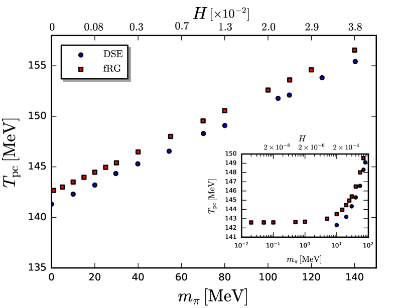
Figure 1: Pseudo-critical temperature $T_{\rm pc}$ as a function of the pion mass obtained from functional QCD studies: this work (fRG) and [29] (DSE). Here, $H=m_{l}/m_{s}$ with the strange current quark mass $m_{s}$ fixed at its physical value.

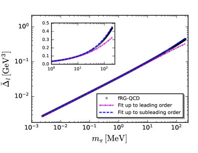
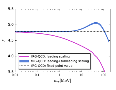
Figure 2: Left panel: Light chiral condensate as a function of the pion mass in comparison to fits based on 5. Right panel: Effective exponent $\delta$ as a function of the pion mass obtained from a scaling analysis of the fRG-QCD data in the left panel. The magenta line denotes the result extracted with only the leading scaling contribution to the chiral condensate in 5, and the blue line includes the sub-leading correction in the pion mass. The blue band shows the error obtained from the uncertainty in determining the sub-leading scaling amplitude $a_{m}$. The dashed line indicates the critical exponent obtained from the fixed-point analysis of the fRG flows. For pion masses within the critical region the curves $\delta(m_{\pi})$ must agree with this exponent.

In Figure 1 we show our results for $T_{\rm pc}(m_{\pi})$. Both methods show excellent agreement. The fRG setup is explained in detail in [7] and details on the DSE computation can be found in [29], see also [30] for a further very recent DSE study. By fitting these results according to 3 across the whole range of available masses, one finds $T_{c,{\rm fRG}}=142.568$ MeV, $T_{c,{\rm DSE}}=141.3$ MeV, $c_{\rm fRG}=0.08924$, $c_{\rm DSE}=0.09581$, $p_{\rm fRG}=1.024$, and $p_{\rm DSE}=0.9606$. We note that the DSE setups used to date do not accommodate the dynamical feedback of the critical mode, and we therefore expect mean-field behaviour in the critical region in this case, i.e., $p_{\rm MF}=4/3$. This is an important observation regarding scaling analyses in general since it makes clear that the superficial agreement of results from different methods including the individual fit values for $c$ and $p$ and the effectively linear scaling of $T_{\rm pc}(m_{\pi})$ across many scales even beyond the physical point does not reveal critical behaviour at all.

We corroborate this result by a direct investigation of the scaling behaviour of the chiral condensate using our fRG setup. Such an analysis is much cleaner since, in contrast to the pseudocritical temperature, the chiral condensate is directly related to a universal scaling function. To this end, we compute the light chiral condensate $\bar{\Delta}_{l}(m_{\pi})$ for a range of pion masses spanning five orders of magnitude, $m_{\pi}\in[0.002,200]$ MeV. This is shown in the left plot of Figure 2. In order to study criticality we expand the magnetic equation of state at $T_{c}$ about $m_{\pi}=0$. The chiral condensate in the critical region is then described by [14]

$$\bar{\Delta}_{l}^{\rm(crit)}(m_{\pi})=B_{c}\,m_{\pi}^{2/\delta}\big{(}1+a_{m}m_{\pi}^{2\theta_{H}}\big{)}\,,$$ (5)

Here, we also included the sub-leading corrections to scaling, which is described by the universal exponent $\theta_{H}$. We emphasise that an accurate determination of the critical temperature $T_{c}$ is crucial for the validity of this expression. Otherwise, the leading correction due to deviations from $T_{c}$, which is $\sim m_{\pi}^{-2/\beta\delta}(T-T_{c})$, needs to be taken into account. It is obtained by expanding the scaling form $\bar{\Delta}_{l}^{\rm(crit)}=m_{\pi}^{2/\delta}f_{G}(z)$ about $t=0$. The procedure of determining $T_{c}$ with high precision is detailed in the supplement. If the system is in the critical region for sufficiently small $m_{\pi}\leq m_{\pi,\rm{crit}}$, the exponents $\delta$ and $\theta_{H}$ are universal, while the amplitudes $B_{c}$ and $a_{m}$ are not. In the critical region the chiral condensate is described accurately by 5 with a fixed set of fit parameters for all $m_{\pi}\leq m_{\pi,\rm{crit}}$. In fact, the size of the critical region can be defined unambiguously through this criterion.

To be specific, within the critical region, 5 should accurately describe our data with the exponents in 4 and fixed coefficients $B_{c}$ and $a_{m}$. In particular, at $T_{c}$ the critical exponent $\delta$ is determined from

$$\ln\frac{\bar{\Delta}_{l}(m_{\pi})}{1+a_{m}m_{\pi}^{2\theta_{H}}}=\frac{1}{\delta}\ln m_{\pi}^{2}+\ln B_{c}\,.$$ (6)

Note that this slope is independent of the leading amplitude $B_{c}$. If only the leading scaling contributions are taken into account, i.e., neglecting the second term in 6, we can use our results for $\bar{\Delta}_{l}(m_{\pi})$ shown in the left plot of Figure 2 to extract the slope of 6. The resulting effective exponent $\delta(m_{\pi})$ is shown as the magenta line in the right plot of Figure 2. To guide the eye, the dashed line shows the value of the actual critical exponent $\delta$ of our system, see 4. In the critical region $\delta(m_{\pi})$ must be independent of the mass and agree with this value. For the leading scaling behaviour this requires $m_{\pi}\lesssim 0.01$ MeV.

We conclude that the leading scaling behaviour can only be valid extremely close to the critical point. Within any reasonable numerical accuracy, sub-leading corrections can usually not be neglected. To take these corrections into account, we need to determine the sub-leading amplitude $a_{m}$. To estimate the underlying uncertainty, we extract it from fitting our data of $\bar{\Delta}_{l}(m_{\pi})$ with 5 and the exponents in 4 in the range $m_{\pi}\in[0.01,m_{\pi,{\rm max}}]$ for two upper values $m_{\pi,{\rm max}}=0.1$ and 10 MeV. With the sub-leading exponent $\theta_{H}$ from 4, we can then use the full equation 6 to extract $\delta(m_{\pi})$ from our data. This is shown by the blue band in the right plot of Figure 2. The boundaries of this band are obtained by using the sub-leading amplitudes $a_{m}$ extracted from the two different fit ranges defined above. We define the critical region as the range of pion masses where the resulting inverse slope $\delta(m_{\pi})$ agrees with the actual exponent and find

$$m_{\pi,{\rm crit}}\approx 2-5\,{\rm MeV}\,.$$ (7)

This result is rather insensitive to the precise value of $a_{m}$. In the supplement we present an error-based analysis of the critical region which yields a compatible result. Hence, as a main result of this work, we observe critical behaviour only for extremely light pions. The physical point of QCD is far away from $O(4)$-criticality. This analysis also extends to the size of the critical region in temperature direction, which we estimate with $T-T_{c}\lesssim 1-7$ MeV. We have deferred the respective analysis to the supplement as, while very interesting, it is beyond the main scope of the present work.

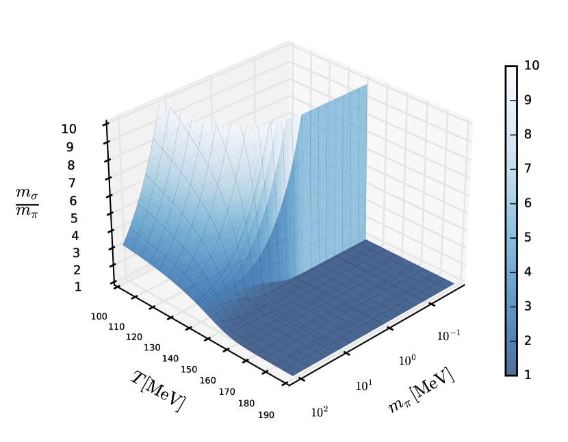
Figure 3: Ratio of the $\sigma$ and $\pi$ meson masses $m_{\sigma}/m_{\pi}$ as a function of the temperature and the pion mass. The system has soft pion modes where this ratio is larger than one.

Soft modes.– Our results clearly show that QCD does not show critical behaviour near the physical point at vanishing chemical potential. Universality is driven by nearly massless critical modes. However, even without such critical modes, the presence of other soft modes, such as pseudo-Goldstone bosons, can significantly alter the dynamical behaviour of QCD, see, e.g., [31, 12, 13]. Below, we shall show that soft modes drive the physics of the QCD phase transitions beyond the critical regime.

In the chiral limit, pions are exactly massless in the broken phase, since they are the Goldstone bosons of chiral symmetry breaking. In this case the phase transition is of second order and the pions and the sigma mode are massless at $T_{c}$. For non-vanishing light current quark masses, the pions acquire an explicit mass $m_{\pi}^{2}\sim m_{l}$ in the broken phase. Still, for sufficiently small light quark masses they remain light in comparison to the other mass scales in QCD. In fact, they are the lightest particles in the low-energy spectrum of QCD [32]. This facilitates the construction of systematic effective field theories such as chiral perturbation theory [33].

Hence, at low energies the structure of QCD is dominated by these soft modes. It is accurately described by pion exchange and the resulting effective theory is organised around the systematic expansion in powers of momenta $p^{2}$, which are, as a result of pion pole dominance, of the order of $m_{\pi}^{2}$. Such an expansion breaks down once $p^{2}$ or $m_{\pi}^{2}$ is of the order of the next-lowest resonances, which are the kaons and the $\sigma$ mesons . If this is the case, exchange processes involving these particles become dominant. Since $1/m_{\pi}$ describes the correlation length of pions, the ratio $m_{\sigma/K}/m_{\pi}$ can be used as a measure of the softness of the pions: If this ratio is greater than one, chiral expansions are justified.

These arguments are straightforward to verify in vacuum and for quantities that can be computed in Euclidean spacetime such as the equation of state in thermal equilibrium. The situation is more subtle for real-time and transport properties. In this case, the vanishing frequency limit and the vanishing spatial momentum limit do not commute in a medium. A small-momentum expansion, as in chiral effective field theory, is therefore not guaranteed to be well-defined. Physically, this phenomenon is due to Landau damping, which gives rise to branch cuts whose location depends on the difference of particle energies [35, 36]. For small mass differences, these cuts are present at small momenta. This not only means that simple small-momentum expansions in general cannot converge at finite $T$, but also that heavy particles can contribute to physical quantities through low-lying thresholds for exchange processes with the heat bath. However, for every particle going on shell in such processes, there is always an off-shell contribution of at least one other particle. This naturally suppresses these contributions from heavy particles, as low-lying thresholds from heavy particles need to involve at least two heavy particles with a small mass difference. Relative to equivalent processes from light particles, the suppression is on the order of the ratio of light over heavy particle masses. Thus, although the systematic low-momentum expansion of chiral effective field theory is not always well-defined, low energy processes in QCD both in Euclidean and Minkowski space are still dominated by the lightest modes in the spectrum.

Naturally, the most striking example is provided by the critical region, which is exactly described by critical modes only. More importantly, a soft mode expansion, i.e., an expansion in terms of fluctuations of the lightest effective degrees of freedom is far more general and is a powerful way to accurately describe the low-energy sector of QCD even beyond the critical regime.

The fRG setup used in the present work is geared towards describing the chiral phase structure of QCD, which is dominated by the light quarks. Consequently, $m_{\sigma}$ can be determined more accurately than $m_{K}$ in the present set-up. Hence, we use the ratio $m_{\sigma}/m_{\pi}$ as a measure for the validity of soft mode expansions. The result is shown in Figure 3 as a function of $T$ and the pion mass $m_{\pi}$, where the strange current quark mass is kept at its physical value and only $m_{l}$ is varied.

We see that $m_{\sigma}/m_{\pi}$ rapidly rises for temperatures below $T_{\rm pc}$. In order to find a reasonable criterion to define the range of validity of soft mode expansions, we first consider the expectations for $m_{\sigma}/m_{\pi}$ in the critical region $H\in[0,H_{\rm crit}]$. In this region the ratio of the masses is universal and can be extracted from the numerical results in [37]. The largest value for this ratio at $z\geq 0$ is reached at $T=T_{c}$, where one finds $\big{(}m_{\sigma}/m_{\pi}\big{)}(H)\big{|}_{H\leq H_{\rm crit}}\approx 2$, independent of $H$. It tends towards one with increasing $z$, e.g., increasing $T$ for fixed $H$. Thus at the pseudocritical temperature in the critical region one has

$$1<\left.\frac{m_{\sigma}}{m_{\pi}}(T_{\rm pc})\right|_{H\leq H_{\rm crit}}\lesssim 2\,.$$ (8)

Since the critical region is certainly well described by a chiral expansion, we conclude that it should be valid whenever $m_{\sigma}/m_{\pi}>1$ for $T\lesssim T_{pc}$ .

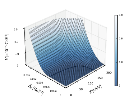
Figure 4: 3D plot of the order parameter potential of QCD as a function of the light quark condensate and the temperature obtained with the fRG.

Order parameter potential.– We have established that hadronic matter around the physical point in QCD is largely controlled by soft pions rather than universality. Thus, while it is certainly appealing to rely on universality for phenomenological applications due to its simplicity, it is unwarranted. Instead of universal scaling functions, non-universal functions are required, and, in general, their computation is much more difficult in QCD. Of particularly broad interest is the order parameter potential $V_{\chi}(T,\bar{\Delta}_{l})$ as it fully characterises the static chiral properties of QCD. In particular, it contains all thermodynamic information as well as all correlations of the order parameter in terms of its derivatives. The latter cannot be extracted from the equation of state, but are indispensable input for dynamic modelling of heavy-ion collisions. For a first application of the use of the full order parameter potential and full propagators in transport equations within a low-energy model, see [38].

Hence, due to its phenomenological relevance, we close this work by providing this potential, first phenomenological applications are beyond the scope of the present work and will be provided elsewhere.

It has been shown in [29] how to compute the order parameter potential from the quark-mass dependence chiral condensate or rather its susceptibility. Here, we briefly recapitulate the important steps: $V_{\chi}(T,\bar{\Delta}_{l})$ is the Legendre transformation of the grand potential $\Omega(m_{l},T)$ with respect to the light quark mass parameter $m_{l}$,

$$V_{\chi}(T,\bar{\Delta}_{l})=\sup_{m_{l}}\Bigl{[}m_{l}\,\bar{\Delta}_{l}-\Omega(T,m_{l})\Bigr{]}\,,$$ (9)

with the chiral condensate $\bar{\Delta}_{l}$ defined in 1 and 2. Equation 9 implies $\partial V_{\chi}/\partial\bar{\Delta}_{l}=\,m_{l}$ and the $\bar{\Delta}_{l}$-integral of this relation provides us with $V_{\chi}$,

$$V_{\chi}(\bar{\Delta}_{l})=\int_{\bar{\Delta}_{l,\chi}(T)}^{\bar{\Delta}_{l}}d\bar{\Delta}\,m_{l}(\bar{\Delta},T)\,.$$ (10)

The integral in 10 requires the knowledge of $m_{l}(\bar{\Delta},T)$, which is obtained from $\bar{\Delta}_{l}(m_{l},T)$ in 1 by inversion. In turn, for $\bar{\Delta}<\bar{\Delta}_{l,\chi}$ we have

$$V_{\chi}(\bar{\Delta}_{l},T)=V_{\chi}(\bar{\Delta}_{l,\chi},T)\,,$$ (11)

due to convexity of $V_{\chi}$ as a Legendre transform.

The numerical result for the effective potential from fRG-QCD is displayed in Figure 4. That from the DSE computation is in quantitative agreement with the fRG result, which follows already from the quantitative agreement of the results for the renormalised condensate and its susceptibility from both methods, see, e.g., [29].

Conclusions.– We have shown that the chiral crossover of QCD with physical quark masses is about two orders of magnitude in the pion mass away from the critical region of the chiral phase transition. We emphasise that a small scaling region facilitates accurate extrapolations based on non-critical data obtained, e.g., from heavy-ion experiments. However, around and below the pseudocritical temperature soft modes still dominate relevant physical aspects of the system. This is encoded in the order parameter potential, which we computed here from functional approaches to QCD. This is the basis for beyond Ginzburg-Landau type analyses of the chiral crossover regime in QCD and a crucially important input for transport studies of the physics of Heavy-Ion collisions.

Acknowledgements.– We thank B. Brandt, H. T. Ding, C.S. Fischer, O. Philipsen and C. Schmidt for discussions. This work is done within the fQCD collaboration [39] and is funded by the National Natural Science Foundation of China under Grant No. 12175030, the Deutsche Forschungsgemeinschaft (DFG, German Research Foundation) under Germany’s Excellence Strategy EXC 2181/1 - 390900948 (the Heidelberg STRUCTURES Excellence Cluster) and the Collaborative Research Centre SFB 1225 - 273811115 (ISOQUANT), and the Collaborative Research Centers TransRegio CRC-TR 211 “Strong-interaction matter under extreme conditions”– project number 315477589 – TRR 211. Moreover, JB acknowledges support by the DFG under grant BR 4005/6-1 (Heisenberg program).

Supplemental Material

S.1 Scaling solution of QCD flows

Here we describe how we compute the critical exponents from the scaling solution of the fRG flow equations. The general strategy is to find the Wilson-Fisher fixed point associated to the second-order phase transition in the chiral limit. Scale invariance at this fixed point implies that the non-perturbative RG flow equations, which describe the RG-scale dependence of the (dimensionless) effective couplings, are zero. From this requirement, fixed point values for all couplings of the theory can be determined. By considering small deviations from these values, relevant (infrared-repulsive) and irrelevant (infrared-attractive) directions in the space of all running couplings can be identified and critical exponents can be extracted from their scaling with the RG scale $k$.

The full set of equations is given in the appendices of  [7]. Various simplifications can be made for the scaling analysis. Since we are considering a thermal phase transition, all fermionic degrees of freedom decouple and QCD reduces to a three-dimensional system of bosonic degrees of freedom. We emphasise that this not only entails gluons, but also bosonic resonances/bound states that are relevant in the vicinity of the phase transition. Formally, this is most easily seen in the Matsubara formalism of finite temperature field theory, where bosonic Euclidean frequencies are $2\pi nT/k$ and fermionic frequencies are $(2n+1)\pi T/k$ with $n\in\mathbb{Z}$. The scaling regime is reached in the deep infrared for $k\rightarrow 0$. Thus, at finite $T$ we have $T/k\rightarrow\infty$. Fermions do not have a Matsubara zero mode, but instead acquire a thermal mass $m_{\psi}/k\sim\pi T/k$ and hence decouple in the scaling regime. Similarly, all finite Matsubara modes of bosons decouple and only the zero mode with vanishing frequency survives. The resulting system only depends on spatial momenta and is therefore dimensionally reduced to $d=3$ dimensions. This is facilitated by the use of $3d$ spatial regulators here.

In addition, the gluons decouple in the infrared due to their finite mass gap [7]. This leaves only mesons as potential relevant degrees of freedom. In the light chiral limit, all mesons involving strange quarks decouple as well, as they do not become critical at physical strange quark mass. This is hardwired in the present approximation, where the dynamics of these mesons do not feed back into the system of RG flows [7]. The only mesonic interactions that are taken into account self-consistently stem from the scalar-pseudoscalar quark interaction channel, which gives rise to the pions and the $\sigma$ meson, i.e.,

$$(\bar{q}q)^{2}+(\bar{q}\,i\gamma_{5}\boldsymbol{\sigma}q)^{2},$$ (12)

with the Pauli-matrices $\boldsymbol{\sigma}$ in light-flavour space. The axial anomaly enters through the explicit breaking of $U_{A}(1)$ of this interaction channel. Thus, also the $\eta^{\prime}$ meson is always massive in our case and decouples in the critical region. Lastly, we consider only cutoff scale $k$-dependent meson wave functions instead of taking into account the full momentum dependence.

In summary, our system of QCD flow equations exactly reduces to that of the 3$d$ $O(4)$ model in the LPA^′ truncation described below: The RG flow of the scale-dependent effective potential $U_{k}(\rho)$, with $\rho=\phi^{2}/2$ and the $O(4)$ vector field $\phi=(\sigma,\boldsymbol{\pi})$, in its scaling form is given by [40]

$$\partial_{t}u_{k}(\bar{\rho})=-du_{k}(\bar{\rho}_{k})+(d-2+\eta)\bar{\rho}_{k}u_{k}^{\prime}(\bar{\rho}_{k})+\frac{1}{2^{d-1}\pi^{d/2}\,d\,\Gamma\big{(}\frac{d}{2}\big{)}}\,\bigg{(}\frac{N-1}{1+u_{k}^{\prime}(\bar{\rho}_{k})}+\frac{1}{1+u_{k}^{\prime}(\bar{\rho}_{k})+2\bar{\rho}u_{k}^{\prime\prime}(\bar{\rho}_{k})}\bigg{)}\,,$$ (13)

with $\partial_{t}=k\frac{d}{dk}$, $d=3$ and $N=4$. We defined $u_{k}(\bar{\rho}_{k})=k^{-d}U\big{(}k^{d-2}Z_{\pi,k}^{-1}\,\bar{\rho}_{k}\big{)}$ and the dimensionless, renormalised field $\bar{\rho}_{k}=k^{2-d}Z_{\pi,k}\,\rho$, where $Z_{\pi,k}$ is the wave function of the pion. The anomalous dimension $\eta$ is given by

$$\eta =-\frac{\partial_{t}Z_{\pi,k}}{Z_{\pi,k}}=\frac{\bar{\rho}_{0,k}[u^{\prime\prime}(\bar{\rho}_{0,k})]^{2}}{2^{d-2}\pi^{d/2}\Gamma\big{(}\frac{d+2}{2}\big{)}}\,\frac{1}{[1+2\bar{\rho}u_{k}^{\prime\prime}(\bar{\rho}_{0,k})]^{2}}\,.$$ (14)

In 14, $\bar{\rho}_{0,k}$ is the running minimum of the scale-dependent effective potential, i.e., the solution of the cutoff-scale dependent equation of motion

$$u_{k}^{\prime}(\bar{\rho}_{0,k})=0\,.$$ (15)

The critical effective potential $u^{*}$ follows from scale invariance at the fixed point,

$$\partial_{t}u_{k}(\bar{\rho})\big{|}_{u=u^{*}}=0\,.$$ (16)

Equation 13 is a partial differential equation which we reduce to a coupled set of ordinary equations by expanding the potential about its minimum,

$$u(\bar{\rho})=\sum_{n=2}^{N_{u}}\frac{\lambda_{n,k}}{n!}(\bar{\rho}-\bar{\rho}_{0,k})^{n}\,.$$ (17)

The ansatz 17 is valid in the chiral limit. Away from it, we need to take into account a linear symmetry breaking source $-c_{\sigma}\sigma$, with $c_{\sigma}$ being directly related to the current quark mass. We emphasise, however, that the second order transition in our case occurs in the chiral limit. This follows from the fact that we can exactly reduce our set of QCD flows to the 3$d$ $O(4)$ model in the scaling regime. The fixed point equation 16 then reduces to a set of fixed point equations for the couplings $\lambda_{n,k}$ and the minimum $\bar{\rho}_{0,k}$. We use $N_{u}=5$ throughout this work. Solving these equations using Newton’s method yields the following fixed point values,

$$\bar{\rho}_{0}^{*}=0.07149\,,\qquad\bar{\lambda}_{2}^{*}=4.612\,,\qquad\bar{\lambda}_{3}^{*}=29.70\,,\qquad\bar{\lambda}_{4}^{*}=86.34\,,\qquad\bar{\lambda}_{5}^{*}=-1147\,.$$ (18)

We emphasise that the fixed point values are not universal. But we can use them to extract the anomalous dimension by plugging them into 14 and find

$$\eta=0.0373\,.$$ (19)

To extract further universal quantities, we perturb the couplings $\boldsymbol{g}=(\bar{\rho}_{0,k},\lambda_{2,k},\lambda_{3,k},\lambda_{4,k},\lambda_{5,k})$ around their fixed point values, $\boldsymbol{g}=\boldsymbol{g}^{*}+\delta\boldsymbol{g}$, and consider the linearised flow for small perturbations,

$$\partial_{t}\delta\boldsymbol{g}\approx M^{*}\,\delta\boldsymbol{g}\,,$$ (20)

where we used $\partial_{t}\boldsymbol{g}^{*}=0$. $M^{*}$ is the stability matrix of the set of RG flows,

$$M^{*}_{ij}=\frac{\partial(\partial_{t}g_{i})}{\partial g_{j}}\bigg{|}_{\boldsymbol{g}=\boldsymbol{g}^{*}}\,.$$ (21)

Note that the flows $\partial_{t}g_{i}$ contain the anomalous dimension specified in 19. The eigenvalues $\tilde{m}_{i}$ of the stability matrix determine the scaling of the couplings in the vicinity of the fixed point. The eigendirection $\delta\tilde{g}_{i}$ corresponding to the eigenvalue $\tilde{m}_{i}$ scales as

$$\delta\tilde{g}_{i}(k)\sim k^{\tilde{m}_{i}}\,.$$ (22)

The eigenvalues $\tilde{m}_{i}$ are universal critical exponents. For $\tilde{m}_{i}<0$, the corresponding eigendirection is infrared-repulsive, while the directions with $\tilde{m}_{i}>0$ are infrared-attractive. This defines relevant and irrelevant directions in the RG flow, respectively. The eigenvalues are in general complex, but we find three real ones,

$$\tilde{m}_{1}=-1.280\,,\qquad\tilde{m}_{2}=0.6745\,,\qquad\tilde{m}_{3}=2.722\,.$$ (23)

Hence, we find one relevant direction. Note, however, that we already used that this fixed point occurs in the chiral limit. Thus, there are actually two relevant directions, with the current quark mass being the second. To reach the second order transition, two parameters, the quark mass and, e.g., the temperature need to be fine-tuned. The relevant eigenvalue corresponds to the scaling of the screening mass of the critical mode and is therefore directly related to the correlation length exponent,

$$\nu=-\frac{1}{\tilde{m}_{1}}=0.781\,.$$ (24)

With two relevant universal exponents, $\eta$ and $\nu$, known, we can determine all other relevant critical exponents using scaling relations. For the present purposes, we need $\beta$ and $\delta$, which we get from

$$\beta=(d-2+\eta)\frac{\nu}{2}\,,\qquad\qquad\delta=\frac{d+2-\eta}{d-2+\eta}\,.$$ (25)

The smallest irrelevant eigenvalue in 23 gives the most important sub-leading critical exponent,

$$\omega=\tilde{m}_{2}=0.6745\,.$$ (26)

and the sub-leading exponent used in the next-to-leading order (NLO) scaling analysis in main text is defined by

$$\theta_{H}=\frac{\nu\omega}{\beta\delta}=0.272\,.$$ (27)

Using the relations in 25 and 27 with the universal numbers in 19, 24 and 26 yields the exponents used in the main text in 4. With the second smallest irrelevant exponent in 23 we can also define the exponent required for a next-to-next-to-leading order (NNLO) scaling analysis,

$$\theta_{3}=\frac{\nu\tilde{m}_{3}}{\beta\delta}=1.097\,.$$ (28)

However, since $\theta_{3}/\theta_{H}\approx 4$, NNLO corrections are negligible.

The values we find are in excellent agreement with the most accurately determined exponents to date, see [18] and references therein. We note that a systematic error analysis requires knowledge of higher-order corrections of the derivative expansion we used in meson sector of QCD. This is beyond the scope of this work. However, the good central values we find here are a testament to the rapid convergence of our truncation scheme.

S.2 Critical and regular contributions to the equation of state

In general, we can express the relation between the chiral condensate and the magnetic equation of state as

$$\Delta_{l}(T,m_{\pi}^{2})=m_{\pi}^{2/\delta}f_{G}(z)+f_{\rm reg}(T,m_{\pi}^{2})\,,$$ (29)

where first term is the singular contribution due to critical scaling and the second term is the regular contribution. While the critical contribution is a function of the scaling variable $z$, the regular part is an analytic function of both $T$ and $m_{\pi}^{2}$ independently. Note that we used that the external field is given by $H\sim m_{l}\sim m_{\pi}^{2}$. Expressing the critical part in terms of the leading and sub-leading scaling contributions leads to 5 if the regular part is neglected. We emphasise that universality can only occur if the latter is true. Since the regular part is analytic, it can be approximated as

$$f_{\rm reg}(T,m_{\pi}^{2})=b_{r}(T)\,m_{\pi}^{2}+\mathcal{O}(m_{\pi}^{4})\,.$$ (30)

We can also use 29 to extract the contribution of the regular part to the pseudocritical temperature in order to generalise 3. To this end, we use that we define $T_{\rm pc}$ through the peak position of the temperature derivative of 29,

$$\frac{\partial\Delta_{l}(T,m_{\pi}^{2})}{\partial T}=m_{\pi}^{2/\delta}f_{G}^{\prime}(z)\frac{m_{\pi}^{-2/\beta\delta}}{T_{\rm c}}+\frac{\partial f_{\rm reg}(T,m_{\pi}^{2})}{\partial T}\,.$$ (31)

Without regular corrections, this leads to a pseudocritical scaling variable $z_{\rm pc}$ with $f_{G}^{\prime}(z_{\rm pc})=0$. A consistent definition of $T_{\rm pc}$ including regular corrections is then given by

$$f_{G}^{\prime}(z_{\rm pc})+T_{\rm c}\frac{\partial f_{\rm reg}(T_{\rm pc},m_{\pi}^{2})}{\partial T}\,m_{\pi}^{2/\beta\delta-2/\delta}=0\,.$$ (32)

We see that the corrections from the regular contributions enter with an additional factor $m_{\pi}^{2/\beta\delta-2/\delta}$ and we can generalise 3 to

$$T_{\rm pc}(m_{\pi}^{2})=T_{\rm c}+c\,m_{\pi}^{2/\beta\delta}+d_{r}(m_{\pi}^{2})\,m_{\pi}^{2/\beta\delta-2/\delta}\,,$$ (33)

where $d_{r}(m_{\pi}^{2})$ is an analytic function related to $f_{\rm reg}$. Similar to 30, expanding this function leads to

$$T_{\rm pc}(m_{\pi}^{2}) =T_{\rm c}+c\,m_{\pi}^{2/\beta\delta}+c_{r}\,m_{\pi}^{2+2/\beta\delta-2/\delta}+\mathcal{O}(m_{\pi}^{4})\,.$$ (34)

This agrees with Equation (8) in [1], and we can use this form for improving the fits for $T_{\rm pc}$. Note that there is no correction to $T_{\rm pc}$ from the sub-leading exponent $\theta_{H}$. This can be seen as follows. The chiral phase transition has two relevant parameters at criticality, which is reflected in the fact that we need to tune both the pion mass and the temperature in order to get to the second-order transition. The relevant parameters correspond to infrared-repulsive directions in the RG flow. The first two sub-leading (irrelevant) exponents correspond to the directions with the weakest infrared-attraction, i.e., the two smallest positive eigenvalues of the stability matrix of the set of RG flows, cf. 23. Taking only the relevant and these first two irrelevant directions into account, the free energy $f$ at criticality depends on three parameters $u_{T}$, $u_{H}$, $u_{2}$ and $u_{3}$ and behaves under rescaling with a scale $b$ as

$$f(u_{T},u_{H},u_{2},u_{3})=b^{-d}f\big{(}u_{T}b^{\frac{1}{\nu}},u_{H}b^{\frac{\beta\delta}{\nu}},u_{2}b^{-\omega},u_{3}b^{-\tilde{m}_{3}}\big{)}\,,$$ (35)

where we used the notation of Section S.1. The parameters $u_{T}$, $u_{H}$, $u_{2}$ and $u_{3}$ are linear combinations of effective couplings of the theory. The powers of $b$ on the right hand side are negative eigenvalues of the stability matrix, which we expressed in terms of known critical exponents. We can choose $b$ to absorb one of the arguments. For the magnetic equation of state $u_{H}$ is chosen, i.e., $b=u_{H}^{-\frac{\nu}{\beta\delta}}$. Then the free energy scaling function becomes a function of only three arguments, $f_{H}(z,w,w_{3})$, with

$$z=u_{T}\,u_{H}^{-\frac{1}{\beta\delta}}\,,\qquad\qquad w=u_{2}u_{H}^{\theta_{H}}\,,\qquad\qquad w_{3}=u_{3}u_{H}^{\theta_{3}}\,.$$ (36)

The parameters $u_{T}$ and $u_{H}$ receive their leading contributions from the reduced temperature $t$ and $m^{2}_{\pi}$. $w$ and $w_{3}$ are sub-leading scaling variables which depend on the irrelevant parameter $u_{2}$ and $u_{3}$ and the exponents $\theta_{H}$ and $\theta_{3}$ defined in Section S.1. Since $\theta_{H},\theta_{3}>0$, the scaling variables $w$ and $w_{3}$ vanish for $m_{\pi}^{2}\rightarrow 0$ and the magnetic scaling function only depends on the leading scaling variable $z$. Note that the dependence of $w$ and $w_{3}$ on $t$ is sub-leading [41], so we neglect these contributions to the magnetic scaling of $T_{\rm pc}$ in the main text.

From the scaling form of the free energy one can derive the magnetic scaling of the order parameter used in the main text. Including NNLO scaling effects it reads

$$\bar{\Delta}_{l}(m_{\pi}^{2})=m_{\pi}^{2/\delta}f_{G}(z,w,w_{3})\,.$$ (37)

We emphasise that the global form of the leading-order scaling function $f_{G}(z)$ is well known, see, e.g., [42] and references therein. Thus at $t=0$ only the leading scaling behavior $\bar{\Delta}_{l}(m_{\pi}^{2})\sim m_{\pi}^{2/\delta}$ is encoded in $f_{G}(z)$. However, for a sensible scaling analysis in an extended region of pion masses at $T_{c}$, sub-leading scaling corrections need to be taken into account. By expanding 37 to leading order in the subleading scaling variables and setting $t=0$ we find

$$\bar{\Delta}_{l}(m_{\pi}^{2})=B_{c}m_{\pi}^{2/\delta}\big{(}1+a_{m}m_{\pi}^{2\theta_{H}}+b_{m}m_{\pi}^{2\theta_{3}}\big{)}+\mathcal{O}\big{(}w^{2},w_{3}^{2}\big{)}\,,$$ (38)

where the coefficients $B_{c}$, $a_{m}$ and $b_{m}$ are related to $f_{G}(z,w,w_{3})$ and its derivatives at $t=0$. As shown in Section S.1, $\theta_{3}$ is much larger than $\theta_{H}$, so that the NNLO scaling correction $\sim m_{\pi}^{2\theta_{3}}$ is negligible. We verified explicitly that the determination of the size of the critical region presented in the main text is completely unaffected by this correction. We can therefore drop it and arrive at the scaling form given in Equation (5) in the main text.

S.3 Critical vs non-critical behaviour

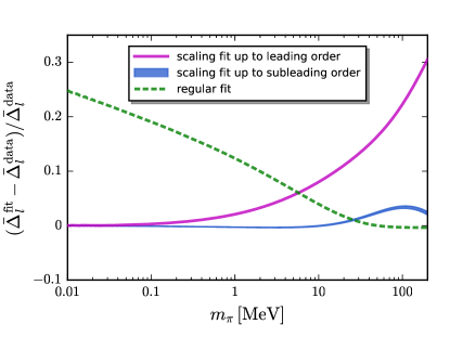
Figure 5: Comparison of errors arising from the scaling and regular fits for the light chiral condensate.

For a precise determination of the critical region, we use that in the critical region for any $m_{\pi}\in[m_{\pi,{\rm min}},m_{\pi,{\rm max}}]$ with $m_{\pi,{\rm min}}<m_{\pi,{\rm max}}\leq m_{\pi,{\rm crit}}$, 5 should accurately describe our data with the exponents in 4 and fixed coefficients $B_{c}$ and $a_{m}$. In contrast, outside of the critical region a non-critical fit should describe our data more accurately. Typically, critical and non-critical contributions are taken into account in a single fit. In this case, the non analytic behaviour related to the phase transition should be stored completely in the critical part of the fit, involving in particular non-natural powers of $m_{\pi}$. All the regular contributions should be analytic and thus are polynomial in $m_{\pi}$. In order to be able to separate critical from non-critical behaviour in a clean way, we do not follow this strategy here. Instead, we use a fit that can only be valid outside the critical region. To this end, we use, as shown in S.5, that the order parameter potential $V(\Delta_{l})$ is well described by a low-order polynomial away from the critical point,

$$V(\Delta_{l})=\lambda_{2}\Delta_{l}^{2}+\lambda_{4}\Delta_{l}^{4}+\lambda_{6}\Delta_{l}^{6}-j\Delta_{l}\,.$$ (39)

The linear source term induces chiral symmetry breaking and is hence related to the pion mass, $j=c\,m_{\pi}^{2}$, with a dimensionful constant $c$ [7, 29]. The resulting equation of motion, $V^{\prime}(\Delta_{l})=0$, thus fixes the relation between the pion mass and the chiral condensate,

$$m_{\pi}^{2}\sim 2\lambda_{2}\Delta_{l}+4\lambda_{4}\Delta_{l}^{3}+6\lambda_{6}\Delta_{l}^{5}\,.$$ (40)

Taking the leading contributions of this relation into account leads us to the following ansatz for the non-critical order parameter,

$$\Delta_{l}^{\rm(reg)}(m_{\pi})=b_{\frac{1}{5}}\,m_{\pi}^{2/5}+b_{\frac{3}{5}}\,m_{\pi}^{6/5}+b_{1}\,m_{\pi}^{2}\,.$$ (41)

We emphasise that this ansatz can only be valid outside the critical region for $m_{\pi}>m_{\pi,{\rm crit}}$. Despite the similarities of some of the exponents in 41 to the critical ones in 5, e.g., $\delta\approx 5$ and $\theta_{H}\approx 0.3$, the branch cuts of $\Delta_{l}^{\rm(reg)}(m_{\pi})$ at $m_{\pi}=0$ are unrelated to the chiral phase transition since the origin lies outside of the range of validity of this function. In fact, it is the similarity of the exponents that makes the analysis of the critical region rather intricate: Without a large amount of high-precision data across a wide range of orders of magnitude, no conclusions about criticality can be drawn.

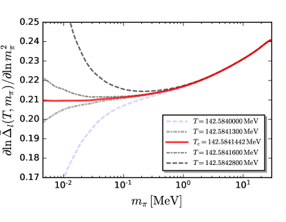
Figure 6: Determination of the critical temperature $T_{c}$ in the chiral limit through the behaviour of $\partial\ln\bar{\Delta}_{l}/\partial\ln m_{\pi}^{2}$ as a function of $m_{\pi}$ at several values of temperature in the vicinity of $T_{c}$.

In the critical region, the mass-dependence of the order parameter is better described by a scaling fit based on 5 with the exponents in 4, while outside the critical region a regular fit based on 41 should yield higher precision. We use both scaling and regular fits for $\Delta_{l}(m_{\pi})$. We employ two scaling fits in order to evaluate the relevance of the subleading scaling term: one fit only includes the leading term and the second one also includes the sub-leading term in 5, similar as in the right panel of Figure 2. The light quark chiral condensate $\Delta_{l}(m_{\pi})$ in the range of $m_{\pi}\in[0.01,0.1]$ MeV is used for the leading-order scaling fit, and those of $m_{\pi}\in[0.01,m_{\pi,{\rm max}}]$ for two upper values $m_{\pi,{\rm max}}=0.1$ and 10 MeV are used for the fit that also includes the sub-leading correction. The regular fits is done with the non-critical ansatz 41 by using $\Delta_{l}(m_{\pi})$ in the range of $m_{\pi}\in[100,200]$ MeV. The resulting errors of the fits across the whole range of data are shown in Figure 5. We find that the error of regular fit is smaller than that of the leading-order scaling fit and that also including the subleading scaling for quark masses larger than $m_{\pi}\approx 6$ MeV and $m_{\pi}\approx 25$ MeV respectively.

We also emphasise that the quality of separate critical and regular fits as shown in Figure 5 is only an indication for where scaling or non-scaling clearly dominates. However, there is a region where a combined fit including both scaling and regular contributions is required to most accurately describe the data. Together with our results of the main text, this region is approximately between 5 and 25 MeV. Crucially, as soon as non-universal regular contributions are necessary to describe the data, the system itself is outside the universal scaling region. As shown in the main text, this occurs for $m_{\pi}\gtrsim 2-5$ MeV. Our result in Figure 5 is fully consistent with this finding. Furthermore, for $m_{\pi}\gtrsim 25$ MeV, no information on scaling is required to accurately describe the data within the accuracy of our results. Importantly, this entails that even with the present high precision data no information about scaling can be extracted from data in this regime.

S.4 Critical temperature in the chiral limit

In Figure 1 in the main text, we have used the pseudo-critical temperature $T_{\mathrm{pc}}$ of the chiral crossover at finite quark mass to extract the critical temperature $T_{c}$ in the chiral limit by utilising 3. One obtains $T_{c}=142.568$ MeV for the fRG results there. This numerical precision of $T_{c}$, however, is not adequate to determine the critical behaviour of the phase transition, e.g., the critical exponents and the size of critical region. This is clearly demonstrated in Figure 6, where $\partial\ln\bar{\Delta}_{l}/\partial\ln m_{\pi}^{2}$ is shown as a function of the pion mass for several values of temperature in the proximity of the critical temperature. Obviously, if the temperature is $T=T_{c}$, the ratio should approach to $1/\delta$, as the red solid line shows. Once the temperature is away from the critical value, it deviates from the red curve quickly in the regime of small $m_{\pi}$. The larger $|T-T_{c}|$ is, the bigger is the $m_{\pi}$ where the deviation takes place. Consequently, one can use this property to determine the critical temperature to a very high precision, $T_{c}=142.5841442$ MeV, that is 10 significant numbers.

The present high precision data also allow us to estimate the size of the critical region in the temperature direction. A full analysis will be presented elsewhere. To this end, we study the dependence of the chiral condensate on the reduced temperature close to the chiral limit at $m_{\pi}=0.002$ MeV. To estimate the size of the critical region in temperature direction we perform a leading order scaling analysis using

$$\Delta_{l}(t)\approx A\,t^{\beta}\,,\qquad\textrm{with}\;\beta\approx 0.405\,,\qquad\textrm{and}\qquad t=\frac{T-T_{c}}{T_{c}}\,.$$ (42)

This form can be derived from the thermal scaling of the scaling function in 35. The exponent is determined in Section S.1. In Figure 7 we show $\ln\bar{\Delta}_{l}$ as a function of the reduced temperature in comparison to $\beta\ln(-t)+\ln A$. Strictly speaking the scaling terminates at about $\ln(-t)\approx-5$, but a sizable overlap still is visible up to $\ln(-t)\approx-3$. This translates into a scaling region in the broken phase with

$$T_{c}-T\lesssim 1-7\,\textrm{MeV}\,,\qquad\textrm{for}\qquad T_{c}-T>0\,.$$ (43)

This is significantly smaller than the respective estimates from lattice QCD in [4] and the very recent DSE study in [30]. The lattice study in [6] finds a scaling region compatible with ours, but owing to a nonzero lattice spacing and the use of staggered fermions, an unphysical $3d$-$O(2)$ scaling is observed. We note that the leading scaling behaviour has also been used in these works. The effect of subleading corrections will be studied in a forthcoming work.

In this context we emphasise once more that our present scaling analysis in functional QCD and the preceding one in [8] comes with two indispensable properties that are ultimately required to make conclusive predictions on the scaling and the size of the scaling regime:

• Scaling is generated dynamically.

• Scaling properties of QCD are obtained for all masses with sufficiently high precision.

While (1) is also present in lattice studies, the combination of (1) & (2) can presently only be achieved within lattice simulations for large pion masses that are far outside the range of pion masses where we observe the dominance of critical scaling. Moreover, even with the present high precision data it is impossible to extract scaling properties for pion masses $m_{\pi}\gtrsim 25$ MeV: while they have to be present as subleading corrections, their suppression is too large.

Other functional QCD studies often lack (1). This statement also extends to the dynamics of the soft modes and its back reaction on the dynamics of the other fields.

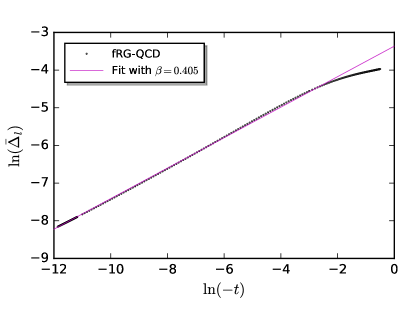
Figure 7: The logarithm of the light chiral condensate $\ln\Delta_{l}$ as a function of the logarithm of (minus) the reduced temperature, see 42.

S.5 Fit of the order parameter potential

The current fRG study gives us direct access to the order parameter potential, whose scaling form in the chiral limit determines all critical properties. Note that this information is only indirectly obtained within lattice simulations, where one has to rely on the computation of correlation functions. They are defined as $m_{q},\mu_{B},...$-derivatives of the order parameter potential which comes along with a loss of accuracy and global information. We find that the dimensionless potential as a function of the light quark condensate in the broken phase can very accurately be parametrised as

$$\bar{V}_{\chi}(\tilde{\Delta}_{l})= \frac{\lambda_{4}}{8}(\tilde{\Delta}_{l}^{2}-\tilde{\Delta}_{l,\chi}^{2})^{2}+\frac{\lambda_{6}}{24}(\tilde{\Delta}_{l}^{2}-\tilde{\Delta}_{l,\chi}^{2})^{3}\,,$$ (44)

with the dimensionless light quark condensate $\tilde{\Delta}_{l}=\bar{\Delta}_{l}/\bar{\Delta}_{l,\chi}(T=0)$, in the chiral limit $\tilde{\Delta}_{l,\chi}=\bar{\Delta}_{l,\chi}/\bar{\Delta}_{l,\chi}(T=0)$, where $\lambda_{4}\geq 0$ and $\lambda_{6}\geq 0$ are assumed. Hence, the squared curvature mass at the minimum reads

$$m_{\Delta_{l}}^{2}= \partial^{2}_{\tilde{\Delta}_{l}}\bar{V}_{\chi}(\tilde{\Delta}_{l}=\tilde{\Delta}_{l,\chi})=\lambda_{4}\tilde{\Delta}_{l,\chi}^{2}\,.$$ (45)

In the symmetric phase the potential is well approximated by

$$\bar{V}_{\chi}(\tilde{\Delta}_{l})= \frac{m_{\Delta_{l}}^{2}}{2}\tilde{\Delta}_{l}^{2}+\frac{\lambda_{4}}{8}\tilde{\Delta}_{l}^{4}+\frac{\lambda_{6}}{24}\tilde{\Delta}_{l}^{6}\,.$$ (46)

We use polynomials to fit the temperature dependence of coefficients in 44 and 46 in the broken and symmetric phase, respectively. The temperature-dependent mass reads

$$m_{\Delta_{l}}^{2}(t)\Big{|}_{-t\in\{0,1\}}=\sum_{n=0}^{n_{max}}a_{n}(-t)^{n}\,,\qquad\qquad m_{\Delta_{l}}^{2}(t)\Big{|}_{t\in\{0,0.39\}}=\sum_{n=0}^{n_{max}}a^{\prime}_{n}t^{n}\,,$$ (47)

The mass is expanded in the reduced temperature $t=(T-T_{c})/T_{c}$ with $t>0$ in the symmetric phase and $t<0$ in the broken phase.The fourth-order coefficients in the broken and symmetric phases are given by

$$\lambda_{4}(t)\Big{|}_{-t\in\{0,1\}}=\sum_{n=0}^{n_{max}}b_{n}(-t)^{n}\,,\qquad\qquad\lambda_{4}(t)\Big{|}_{t\in\{0,0.39\}}=\sum_{n=0}^{n_{max}}b^{\prime}_{n}t^{n}\,.$$ (48)

Finally, rhe sixth-order coefficients in the broken and symmetric phases read

$$\lambda_{6}(t)\Big{|}_{-t\in\{0,1\}}=\sum_{n=0}^{n_{max}}c_{n}(-t)^{n}\,,\qquad\qquad\lambda_{6}(t)\Big{|}_{t\in\{0,0.39\}}=\sum_{n=0}^{n_{max}}c^{\prime}_{n}t^{n}\,.$$ (49)

The numerical results are plotted in Figure 8. They are used to determine the values of coefficients of the polynomials in 47, 48 and 49, and the relevant results are collected in Table 1. This can be used as input for phenomenological applications. We emphasise again that our finding that the order parameter potential away from criticality is well described by a sixth-order polynomial corroborates our choice for the fit to the non-critical order parameter in Section S.3.

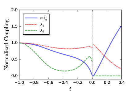
Figure 8: Second, forth and sixth order couplings $m_{\Delta_{l}}^{2}(t)$ and $\lambda_{4,6}(t)$ of the effective potential in Figure 4 as functions of the reduced temperature $t$, normalised to their respective values at $T=0$ for plotting. The numerical values depicted here are used for determining the fit parametes in Table 1.

	$n=0$	1	2	3	4	5	6	7	8
$a$	0	-1.83 $\times 10^{4}$	-7.03$\times 10^{4}$	-1.38$\times 10^{5}$	-1.23$\times 10^{5}$	-4.06$\times 10^{4}$	0	0	0
$a^{\prime}$	0	8.41$\times 10^{3}$	3.27$\times 10^{4}$	-5.63$\times 10^{4}$	0	0	0	0	0
$b$	2.88$\times 10^{3}$	-9.54$\times 10^{2}$	-1.32$\times 10^{4}$	-3.78$\times 10^{4}$	-3.79$\times 10^{4}$	-1.29$\times 10^{4}$	0	0	0
$b^{\prime}$	3.27$\times 10^{3}$	-7.23$\times 10^{3}$	-5.71$\times 10^{3}$	1.95$\times 10^{4}$	0	0	0	0	0
$c$	1.39$\times 10^{5}$	-2.24$\times 10^{6}$	-3.69$\times 10^{7}$	-2.14$\times 10^{8}$	-6.52$\times 10^{8}$	-1.14$\times 10^{9}$	-1.14$\times 10^{9}$	-6.06$\times 10^{8}$	-1.33$\times 10^{8}$
$c^{\prime}$	0	0	0	0	0	0	0	0	0

Table 1: Values of the expansion coefficients of an expansion in the reduced temperature $t$ of the second, forth and sixth order couplings $m_{\Delta_{l}}^{2}(t)$ and $\lambda_{4,6}(t)$ of the effective potential, defined in 47, 48 and 49. The coefficients are computed from a fit to the numerical data presented in Figure 8.

References

- Ding et al. [2019] H. T. Ding et al. (HotQCD), Chiral Phase Transition Temperature in ( 2+1 )-Flavor QCD, Phys. Rev. Lett. 123, 062002 (2019), arXiv:1903.04801 [hep-lat] .
- Borsanyi et al. [2020] S. Borsanyi, Z. Fodor, J. N. Guenther, R. Kara, S. D. Katz, P. Parotto, A. Pasztor, C. Ratti, and K. K. Szabo, QCD Crossover at Finite Chemical Potential from Lattice Simulations, Phys. Rev. Lett. 125, 052001 (2020), arXiv:2002.02821 [hep-lat] .
- Aarts et al. [2022] G. Aarts et al., Properties of the QCD thermal transition with Nf=2+1 flavors of Wilson quark, Phys. Rev. D 105, 034504 (2022), arXiv:2007.04188 [hep-lat] .
- Kotov et al. [2021] A. Y. Kotov, M. P. Lombardo, and A. Trunin, QCD transition at the physical point, and its scaling window from twisted mass Wilson fermions, Phys. Lett. B 823, 136749 (2021), arXiv:2105.09842 [hep-lat] .
- Aarts et al. [2023] G. Aarts et al., Phase Transitions in Particle Physics - Results and Perspectives from Lattice Quantum Chromo-Dynamics, in Phase Transitions in Particle Physics: Results and Perspectives from Lattice Quantum Chromo-Dynamics (2023) arXiv:2301.04382 [hep-lat] .
- Ding et al. [2023] H.-T. Ding, W.-P. Huang, S. Mukherjee, and P. Petreczky, Microscopic Encoding of Macroscopic Universality: Scaling properties of Dirac Eigenspectra near QCD Chiral Phase Transition, (2023), arXiv:2305.10916 [hep-lat] .
- Fu et al. [2020] W.-j. Fu, J. M. Pawlowski, and F. Rennecke, QCD phase structure at finite temperature and density, Phys. Rev. D 101, 054032 (2020), arXiv:1909.02991 [hep-ph] .
- Braun et al. [2020] J. Braun, W.-j. Fu, J. M. Pawlowski, F. Rennecke, D. Rosenblüh, and S. Yin, Chiral susceptibility in ( 2+1 )-flavor QCD, Phys. Rev. D 102, 056010 (2020), arXiv:2003.13112 [hep-ph] .
- Hohenberg and Halperin [1977] P. C. Hohenberg and B. I. Halperin, Theory of Dynamic Critical Phenomena, Rev. Mod. Phys. 49, 435 (1977).
- Berdnikov and Rajagopal [2000] B. Berdnikov and K. Rajagopal, Slowing out-of-equilibrium near the QCD critical point, Phys. Rev. D 61, 105017 (2000), arXiv:hep-ph/9912274 .
- Rajagopal and Wilczek [1993] K. Rajagopal and F. Wilczek, Static and dynamic critical phenomena at a second order QCD phase transition, Nucl. Phys. B 399, 395 (1993), arXiv:hep-ph/9210253 .
- Grossi et al. [2020] E. Grossi, A. Soloviev, D. Teaney, and F. Yan, Transport and hydrodynamics in the chiral limit, Phys. Rev. D 102, 014042 (2020), arXiv:2005.02885 [hep-th] .
- Grossi et al. [2021] E. Grossi, A. Soloviev, D. Teaney, and F. Yan, Soft pions and transport near the chiral critical point, Phys. Rev. D 104, 034025 (2021), arXiv:2101.10847 [nucl-th] .
- Zinn-Justin [2002] J. Zinn-Justin, Quantum field theory and critical phenomena, Int. Ser. Monogr. Phys. 113, 1 (2002).
- Braun et al. [2011] J. Braun, B. Klein, and P. Piasecki, On the scaling behavior of the chiral phase transition in qcd in finite and infinite volume, The European Physical Journal C 71, 10.1140/epjc/s10052-011-1576-7 (2011).
- Tetradis and Wetterich [1994] N. Tetradis and C. Wetterich, Critical exponents from effective average action, Nucl. Phys. B 422, 541 (1994), arXiv:hep-ph/9308214 .
- Balog et al. [2019] I. Balog, H. Chaté, B. Delamotte, M. Marohnic, and N. Wschebor, Convergence of Nonperturbative Approximations to the Renormalization Group, Phys. Rev. Lett. 123, 240604 (2019), arXiv:1907.01829 [cond-mat.stat-mech] .
- De Polsi et al. [2020] G. De Polsi, I. Balog, M. Tissier, and N. Wschebor, Precision calculation of critical exponents in the universality classes with the nonperturbative renormalization group, Phys. Rev. E 101, 042113 (2020), arXiv:2001.07525 [cond-mat.stat-mech] .
- Dupuis et al. [2021] N. Dupuis, L. Canet, A. Eichhorn, W. Metzner, J. M. Pawlowski, M. Tissier, and N. Wschebor, The nonperturbative functional renormalization group and its applications, Phys. Rept. 910, 1 (2021), arXiv:2006.04853 [cond-mat.stat-mech] .
- Mitter et al. [2015] M. Mitter, J. M. Pawlowski, and N. Strodthoff, Chiral symmetry breaking in continuum QCD, Phys. Rev. D91, 054035 (2015), arXiv:1411.7978 [hep-ph] .
- Braun et al. [2016] J. Braun, L. Fister, J. M. Pawlowski, and F. Rennecke, From Quarks and Gluons to Hadrons: Chiral Symmetry Breaking in Dynamical QCD, Phys. Rev. D94, 034016 (2016), arXiv:1412.1045 [hep-ph] .
- Rennecke [2015] F. Rennecke, Vacuum structure of vector mesons in QCD, Phys. Rev. D92, 076012 (2015), arXiv:1504.03585 [hep-ph] .
- Cyrol et al. [2018] A. K. Cyrol, M. Mitter, J. M. Pawlowski, and N. Strodthoff, Nonperturbative quark, gluon, and meson correlators of unquenched QCD, Phys. Rev. D97, 054006 (2018), arXiv:1706.06326 [hep-ph] .
- Pisarski and Wilczek [1984] R. D. Pisarski and F. Wilczek, Remarks on the Chiral Phase Transition in Chromodynamics, Phys. Rev. D 29, 338 (1984).
- Berges et al. [1999] J. Berges, D. U. Jungnickel, and C. Wetterich, Two flavor chiral phase transition from nonperturbative flow equations, Phys. Rev. D 59, 034010 (1999), arXiv:hep-ph/9705474 .
- Schaefer and Wambach [2005] B.-J. Schaefer and J. Wambach, The Phase diagram of the quark meson model, Nucl. Phys. A757, 479 (2005), arXiv:nucl-th/0403039 [nucl-th] .
- Fukushima [2008] K. Fukushima, Phase diagrams in the three-flavor Nambu-Jona-Lasinio model with the Polyakov loop, Phys. Rev. D 77, 114028 (2008), [Erratum: Phys.Rev.D 78, 039902 (2008)], arXiv:0803.3318 [hep-ph] .
- Resch et al. [2019] S. Resch, F. Rennecke, and B.-J. Schaefer, Mass sensitivity of the three-flavor chiral phase transition, Phys. Rev. D99, 076005 (2019), arXiv:1712.07961 [hep-ph] .
- Gao and Pawlowski [2022] F. Gao and J. M. Pawlowski, Phase structure of (2+1)-flavor QCD and the magnetic equation of state, Phys. Rev. D 105, 094020 (2022), arXiv:2112.01395 [hep-ph] .
- Bernhardt and Fischer [2023] J. Bernhardt and C. S. Fischer, QCD phase transitions in the light quark chiral limit, (2023), arXiv:2309.06737 [hep-ph] .
- Son [2000] D. T. Son, Hydrodynamics of nuclear matter in the chiral limit, Phys. Rev. Lett. 84, 3771 (2000), arXiv:hep-ph/9912267 .
- Zyla et al. [2020] P. A. Zyla et al. (Particle Data Group), Review of Particle Physics, PTEP 2020, 083C01 (2020).
- Gasser and Leutwyler [1984] J. Gasser and H. Leutwyler, Chiral Perturbation Theory to One Loop, Annals Phys. 158, 142 (1984).
- Note [1] We tacitly identify the meson with the resonance, which is customary.
- Arnold et al. [1993] P. B. Arnold, S. Vokos, P. F. Bedaque, and A. K. Das, On the analytic structure of the selfenergy for massive gauge bosons at finite temperature, Phys. Rev. D 47, 4698 (1993), arXiv:hep-ph/9211334 .
- Bellac [2011] M. L. Bellac, Thermal Field Theory, Cambridge Monographs on Mathematical Physics (Cambridge University Press, 2011).
- Engels et al. [2003] J. Engels, L. Fromme, and M. Seniuch, Correlation lengths and scaling functions in the three-dimensional O(4) model, Nucl. Phys. B 675, 533 (2003), arXiv:hep-lat/0307032 .
- Bluhm et al. [2019] M. Bluhm, Y. Jiang, M. Nahrgang, J. M. Pawlowski, F. Rennecke, and N. Wink, Time-evolution of fluctuations as signal of the phase transition dynamics in a QCD-assisted transport approach, Proceedings, 27th International Conference on Ultrarelativistic Nucleus-Nucleus Collisions (Quark Matter 2018): Venice, Italy, May 14-19, 2018, Nucl. Phys. A982, 871 (2019), arXiv:1808.01377 [hep-ph] .
- Braun et al. [2023] J. Braun, Y.-r. Chen, W.-j. Fu, F. Gao, F. Ihssen, A. Geissel, C. Huang, Y. Lu, J. M. Pawlowski, F. Rennecke, F. Sattler, B. Schallmo, J. Stoll, Y.-y. Tan, S. Töpfel, J. Turnwald, R. Wen, J. Wessely, N. Wink, S. Yin, and N. Zorbach, fQCD collaboration, (2023).
- Berges et al. [1996] J. Berges, N. Tetradis, and C. Wetterich, Critical equation of state from the average action, Phys. Rev. Lett. 77, 873 (1996), arXiv:hep-th/9507159 .
- Pelissetto and Vicari [2002] A. Pelissetto and E. Vicari, Critical phenomena and renormalization group theory, Phys. Rept. 368, 549 (2002), arXiv:cond-mat/0012164 .
- Karsch et al. [2023] F. Karsch, M. Neumann, and M. Sarkar, Scaling functions of the three-dimensional Z(2), O(2), and O(4) models and their finite-size dependence in an external field, Phys. Rev. D 108, 014505 (2023), arXiv:2304.01710 [hep-lat] .