Predicting mutational effects on protein-protein binding via a side-chain diffusion probabilistic model

Abstract

Many crucial biological processes rely on networks of protein-protein interactions. Predicting the effect of amino acid mutations on protein-protein binding is vital in protein engineering and therapeutic discovery. However, the scarcity of annotated experimental data on binding energy poses a significant challenge for developing computational approaches, particularly deep learning-based methods. In this work, we propose SidechainDiff, a representation learning-based approach that leverages unlabelled experimental protein structures. SidechainDiff utilizes a Riemannian diffusion model to learn the generative process of side-chain conformations and can also give the structural context representations of mutations on the protein-protein interface. Leveraging the learned representations, we achieve state-of-the-art performance in predicting the mutational effects on protein-protein binding. Furthermore, SidechainDiff is the first diffusion-based generative model for side-chains, distinguishing it from prior efforts that have predominantly focused on generating protein backbone structures.

1 Introduction

Many crucial biological processes, including membrane transport and cell signaling, are likely regulated by intricate networks of protein-protein interactions rather than single proteins acting independently (Calakos et al., 1994; Jones and Thornton, 1996; Levskaya et al., 2009; Schwikowski et al., 2000). One representative example is the interaction between the spike protein of the SARS-CoV-2 virus and its receptor protein ACE2 on the surface of human cells, which is crucial for the virus to invade target cells (Lan et al., 2020). Meanwhile, specific human antibodies, an essential type of protein in the immune system, can prevent the virus entry by competitively binding to the spike protein (Shan et al., 2022).

In protein engineering and therapeutic discovery, it is a crucial step to induce amino acid mutations on the protein-protein interface to modulate binding affinity (T O’Neil and Hoess, 1995). For example, to enhance the efficacy of an antibody against a virus, one practical approach is to introduce amino acid mutations and filter the resulting antibody sequences to increase binding affinity and specificity to the target viral protein (Mason et al., 2021). However, the variant space that can be explored using experimental assays is very limited, and developing an effective high-throughput screening can require a significant experimental effort.

Computational methods have been developed to predict the mutational effect on binding affinity measured by the change in binding free energy (i.e., $\Delta\Delta G$). Traditional computational approaches mostly used physical energy features, such as van der Waals and solvation energy, in combination with statistical models to predict $\Delta\Delta G$ (Schymkowitz et al., 2005; Meireles et al., 2010; Alford et al., 2017; Barlow et al., 2018). The limited model capacity and bias inherent in human-engineered features in these methods hinder their ability to characterize the complex mutational landscape of binding energy. Despite recent breakthroughs in protein modeling with deep learning (Jumper et al., 2021; Baek et al., 2021; Watson et al., 2023), developing deep learning-based models to predict mutational effects on protein-protein binding remains challenging due to the scarcity of labeled experimental data (Jankauskaitė et al., 2019).

Recent studies have investigated various self-supervised learning strategies on protein structures and sequences (Liu et al., 2021; Meier et al., 2021; Hsu et al., 2022; Luo et al., 2023) to ease the data scarcity issue. Among them, GeoPPI (Liu et al., 2021) and RDE (Luo et al., 2023) have focused on optimizing protein side-chain conformations during pre-training, as the side-chain conformations on the protein-protein interface play a critical role in determining binding energy. In protein-protein interactions, the side-chain conformations of amino acids at the interface may exhibit significant variations when comparing the same receptor with different ligands. These side-chain conformations can be more effectively characterized using probability density. Notably, RDE explores a flow-based model to estimate the uncertainty in side-chain conformations and leverages the learned representations to achieve state-of-the-art performance in predicting $\Delta\Delta G$. However, flow-based models possess inherent limitations as they require specialized architectures to construct accurate bijective transformations in probability density (Papamakarios et al., 2021), which results in increased costs associated with model design and implementation.

To address the above limitations, we propose SidechainDiff, a representation learning framework for the protein-protein interfaces. It employs a Riemannian diffusion model to learn the generative process of side-chain conformations and the representation of the structural context of amino acids. To the best of our knowledge, SidechainDiff is the first diffusion probabilistic model for side-chain modeling, whereas previous methods have only focused on protein backbone structures. Furthermore, we leverage the learned representations and neural networks to predict $\Delta\Delta G$.

2 Related Work

2.1 Protein side-chain conformation prediction

Accurate side-chain modeling is essential in understanding the biological functions of proteins. There are two primary categories in predicting protein side-chain conformations: end-to-end full-atom structure prediction methods and side-chain packing. AlphaFold and RoseTTAFold (Jumper et al., 2021; Baek et al., 2021) are two representative methods that simultaneously generate side-chain conformations and backbone structures. In scenarios like structure refinement and protein design, side-packing becomes pivotal. The objective is to determine the conformations of protein side-chains while having their backbone structures already defined. Traditional methods, including Rosetta (Leman et al., 2020) and SCWRL4 (Krivov et al., 2009) operate by minimizing the energy function across a pre-defined rotamer library. Recent methods for side-chain packing often employ deep learning models, such as 3D convolution networks and graph attention networks (McPartlon and Xu, 2023; Misiura et al., 2022; Xu et al., 2022).

Our model distinguishes itself from previous methods for side-chain modelling in two key aspects. First, it’s capable of generating a distribution of side-chain conformations rather than a single conformation. Second, we emphasize side-chain modeling specifically for mutation sites within the protein-protein interface, leveraging the known structural context of these sites.

2.2 Prediction of mutational effects on protein-protein binding

Methods for predicting $\Delta\Delta G$ can be broadly classified into three categories: biophysical methods, statistical methods, and deep learning-based approaches. Biophysical methods offer a robust means of elucidating the molecular mechanisms governing protein-protein interactions and the impact of mutations on these interactions (Schymkowitz et al., 2005; Alford et al., 2017; Steinbrecher et al., 2017). These methods directly integrate information on protein structures and key biophysical properties, such as solvent accessibility, electrostatic potential, and hydrogen bonding patterns. Statistical methods tailor statistical models for the protein properties such as evolutionary conservation and geometric characteristics (Li et al., 2016; Geng et al., 2019; Zhang et al., 2020).

Deep learning-based methods can be categorized into sequence-based methods and structure-based methods. Sequence-based methods primarily either focus on the evolutionary history, multiple sequence alignments (MSAs) in most cases, of the target protein (Hopf et al., 2017; Riesselman et al., 2018; Frazer et al., 2021) or act as protein language models (PLMs) trained on large amounts of protein sequences (Meier et al., 2021; Notin et al., 2022). Structure-based methods can be categorized into end-to-end methods and pre-training-based methods. The end-to-end methods extract features from protein complexes and directly train a neural network model on them (Shan et al., 2022). To mitigate overfitting caused by data sparsity, an alternative approach is to learn representations by pre-training a feature extraction network on unlabeled structures (Liu et al., 2021; Luo et al., 2023). Among them, RDE-Network (Luo et al., 2023) utilizes normalizing flows in torus space to estimate the density of amino acid side-chain conformations and leverages the learned representation to predict $\Delta\Delta G$.

2.3 Diffusion probabilistic models

Diffusion Probabilistic Models (DPMs) are generative models to transform a sample from a tractable noise distribution towards a desired data distribution with a gradual denoising process (Sohl-Dickstein et al., 2015; Kingma et al., 2021; Dhariwal and Nichol, 2021). DPMs have achieved impressive results in generating various data types, including images (Ho et al., 2020; Nichol and Dhariwal, 2021), waveforms, and discrete data like text (Hoogeboom et al., 2021). DPMs-based autoencoders have also been proposed to facilitate representation learning for image data (Preechakul et al., 2022; Zhang et al., 2022).

Inspired by these progresses, DPMs have also been explored in protein modeling, including de novo protein design (Watson et al., 2023; Ingraham et al., ; Yim et al., 2023), motif-scaffolding (Trippe et al., 2023), and molecular dynamics (Arts et al., 2023; Wu and Li, 2023). While the existing methods utilize DPMs for generating protein backbones, a research gap remains in modeling side-chain conformations, which play a critical role in protein-protein binding. The studies by Jing et al. (2022) and Corso et al. (2023) employ diffusion models for generating torsion angles in the context of small molecular design. In contrast, our research is centered on modeling the torsional angles of protein side-chains. Furthermore, our approach distinguishes itself from their models in terms of how we construct the diffusion process.

3 Methods

Our methods have two main components. We first propose SidechainDiff (Figure 1), which is a diffusion probabilistic model for protein side-chains and can also give the structural context representations of mutations on the protein-protein interface. We then propose DiffAffinity that utilize the learned representations to predict $\Delta\Delta G$. We organize this section as follows: Section 3.1 presents the preliminaries and notations that are used throughout the paper and formally defines the problem. Section 3.2 and 3.3 describe SidechainDiff and DiffAffinity, respectively. Section 3.4 describes key details in model training.

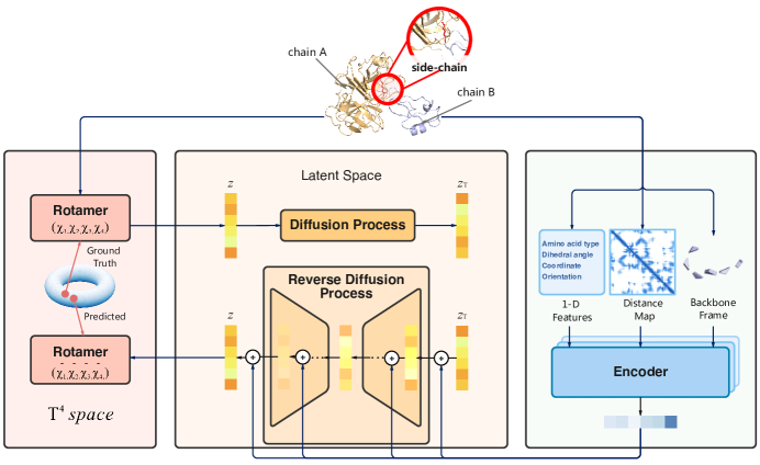
Figure 1: The overall architecture of SidechainDiff.

3.1 Preliminaries and notations

A single-chain protein structure is composed of multiple residues (amino acids). Each amino acid shares a common central carbon atom, called the alpha ($\alpha$) carbon. The alpha carbon is bonded to an amino group (-NH2), a carboxyl group (-COOH), and a hydrogen atom, forming the amino acid’s backbone. Each amino acid has a distinct atom or group bonded to the alpha carbon, known as the side-chain. A residue’s side-chain structure is usually termed a side-chain conformation. The side-chain conformation varies across different amino acids, and it depends on the type of amino acid and the overall protein structure. Our main work focuses on building a generative process of side-chain conformations given the protein backbone structures.

Multiple protein chains bind with each other and form a protein complex. Here we only consider protein complexes with two chains just for notation simplicity and note that our model works for protein complexes with more chains. For a protein complex with $n$ residues, we denote the two chains as chain $A$ and $B$, and the set of its residues as $\{1,...,n\}$. The properities of the $i$-th amino acid include the amino acid type $a_{i}\in\{1,\dots,20\}$, the orientation $\mathbf{R}_{i}\in SO(3)$, the 3D coordinates $\mathbf{x}_{i}\in\mathbb{R}^{3}$, and the side-chain torsion angles $\bm{\chi}_{i}=(\chi_{i}^{(k)})_{k=1}^{4}$ where $\chi_{i}^{(k)}$ belongs to $[0,2\pi)$.

The bond lengths and bond angles in side-chains are usually considered fixed and given backbone structures, we can solely use $\bm{\chi_{i}}$ to reconstruct the coordinates of each atom in a side-chain. Thus, a side-chain conformation is also called a rotamer, which is parameterized with $\bm{\chi_{i}}$. The number of torsional angles ranges from 0 to 4, depending on the residue type. Here, we place a rotamer in a $4$-dimensional torus space $\mathbb{T}^{4}=(\mathbb{S}^{1})^{4}$ where $\mathbb{S}^{1}$ denotes a unit circle.

3.2 SidechainDiff: side-chain diffusion probabilistic model

SidechainDiff utilizes a conditional Riemannian diffusion model in $\mathbb{T}^{4}$ to build the generative process of the four rotamers and estimate their joint distributions (Figure 1). The generative process is conditioned on the structural context of mutations on the protein-protein interface, which is encoded using a SE(3)-invariant neural network. The learned conditional vectors serve as a natural representation of the structural context.

Conditional diffusion probabilistic model on $\mathbb{T}^{4}$    We adopt the continuous score-based framework on compact Riemannian manifolds (De Bortoli et al., 2022) to construct the generative process for rotamers within $\mathbb{T}^{4}$. Our primary adaptation involves conditioning our diffusion model on vectors that are concurrently learned via an encoder network.

Let the random variable $\mathbf{X}$ denote the states of rotamers. And let $(\mathbf{X}_{t})_{t\in[0,T]}$ and $(\mathbf{Y}_{t})_{t\in[0,T]}=(\mathbf{X}_{T-t})_{t\in[0,T]}$ denote the diffusion process and associated reverse diffusion process in $\mathbb{T}^{4}$, respectively. The stochastic differential equation (SDE) and reverse SDE (De Bortoli et al., 2022; Song et al., 2021) can be defined as follows:

$$\mathrm{d}\mathbf{X}_{t}=\mathrm{d}\mathbf{B}_{t}^{\mathcal{M}}.$$ (1)

$$\mathrm{d}\mathbf{Y}_{t}=\nabla\log p_{T-t}(\mathbf{Y}_{t}|\mathbf{Z})\mathrm{d}t+\mathrm{d}\mathbf{B}_{t}^{\mathcal{M}}.$$ (2)

Here, $\mathbf{B}_{t}^{\mathcal{M}}$ represents the Brownian motion on $\mathbb{T}^{4}$, which is approximated with a Reodesic Random Walk (GRW) on $\mathbb{T}^{4}$ (Algorithm 1). The score $\nabla\log p_{T-t}(\mathbf{Y}_{t}|\mathbf{Z})$ in Equation 2 is estimated with a score network $s_{\theta}(\mathbf{X},t,\mathbf{Z})$. We introduce the conditional vector $\mathbf{Z}$ in the score, parameterized with an encoder network that takes the structural context of mutation sites as inputs. We will delve into these components separately in the following subsections.

Geodesic Random Walk in $\mathbb{T}^{4}$     When approximating the Brownian motion on the compact Riemannian manifolds using GRWs, a crucial step is defining the projection map and the exponential map that establishes the connection between the ambient Euclidean space and the associated tangent space, as discussed in previous studies (Jørgensen, 1975; De Bortoli et al., 2022). In the context of $\mathbb{T}^{4}$, which is constructed as the quadruple product of $\mathbb{S}^{1}$ within the ambient Euclidean space $\mathbb{R}^{2}$, it is adequate to focus on modeling Brownian motion on $\mathbb{S}^{1}$, defined as follows:

$$\mathrm{d}\mathbf{x}_{t}=\mathbf{K}\cdot\mathrm{d}\mathbf{B}_{t},\quad\mathbf{K}=\left(\begin{array}[]{cc}0&-1\\ 1&0\end{array}\right).$$ (3)

Here, $\mathbf{B}_{t}$ represents the Brownian motion on the real line in the ambient Euclidean space $\mathbb{R}^{2}$, and $\mathbf{K}$ denotes the diffusion coefficient.

Similarly, the projection map $\mathrm{Proj}_{\mathbf{Y}_{k}^{\gamma}}$ within the tangent space $T_{\mathbf{Y}_{k}}(\mathbb{T}^{4})$ and the exponential map $\mathrm{Exp}$ on $\mathbb{T}^{4}$ can be derived by applying the Cartesian product of the maps designed for $\mathbb{S}^{1}$. To be more precise, these two maps are defined as follows:

$$\mathrm{exp}_{\mathbf{\mu}}(\mathbf{v})=\cos(\|\mathbf{v}\|)\bm{\mu}+\sin(\|\mathbf{v}\|)\frac{\mathbf{v}}{\|\mathbf{v}\|}.$$ (4)

$$\mathrm{proj}_{\bm{\mathbf{\mu}}}(\mathbf{z})=\mathbf{z}-\frac{<\bm{\mu},\mathbf{z}>}{\|\bm{\mu}\|^{2}}\bm{\mu}.$$ (5)

Here, $\bm{\mu}\in\mathbb{S}^{1}$, $\mathbf{v}\in T_{\bm{\mu}}(\mathbb{S}^{1})$, and $\mathbf{z}\in\mathbb{R}^{2}$.

Algorithm 1 Geodesic Random Walk (GRW) during the sampling phase

1:$T,N,Y_{0}^{\gamma},P,\{a_{i},\mathbf{R}_{i},\mathbf{x}_{i},\bm{\chi}_{i}\}_{i=1}^{127}$

2:$\gamma=T/N$$\triangleright$ Step-size

3:$\mathbf{Z}=\mathrm{Enc}_{\phi^{*}}(\{a_{i},\mathbf{R}_{i},\mathbf{x}_{i},\bm{\chi}_{i}\}_{i=1}^{127})$$\triangleright$ Encode the structural context into hidden representation

4:for $k\in\{0,\dots,N-1\}$ do

5:    $\bar{\mathbf{R}}_{k+1}\sim\mathrm{N}(0,\mathrm{Id})$$\triangleright$ Standard Normal noise in ambient space $(\mathbb{R}^{2})^{4}$

6:    $\mathbf{R}_{k+1}=\mathrm{Proj}_{\mathbf{Y}_{k}^{\gamma}}(\bar{\mathbf{R}}_{k+1})$$\triangleright$ Projection in the Tangent Space $T_{Y_{k}}(\mathbb{T}^{4}$)

7:    $\mathbf{W}_{k+1}=-\gamma s_{\theta}(\mathbf{Y}_{k}^{\gamma},k\gamma,\mathbf{Z})+\sqrt{\gamma}\mathbf{R}_{k+1}$$\triangleright$ Compute the Euler-Maruyama step on tangent space

8:    $\mathbf{Y}_{k+1}^{\gamma}=\mathrm{Exp}_{\mathbf{Y}_{k}^{\gamma}}(W_{k+1})$ $\triangleright$ Move along the geodesic defined by $W_{k+1}$ and $\mathbf{Y}_{k}^{\gamma}$ on $\mathbb{T}^{4}$

9:end for

10:return $\{\mathbf{Y}_{k}^{\gamma}\}_{k=0}^{N}$

Score network    The architecture of the score network $s_{\theta}(\mathbf{X},t,\mathbf{Z})$ is implemented as a three-layer Multilayer Perceptron (MLP) with 512 units in each layer. It takes as inputs the conditional vector from the encoder network representing the structural context of the mutations, the sampled rotamers, and the timestep $t$.

Conditional encoder network    The encoder network (Figure S1) takes as inputs both single features, consisting of amino acid type, backbone dihedral angles, and local atom coordinates for each amino acid, as well as pair features such as pair distances and relative positions between two amino acids. An SE3-invariant IPA network (Jumper et al., 2021) is utilized to obtain the conditional vector $\mathbf{Z}$ for the structural context of the mutations. Further information regarding the encoder can be found in App. A.1.

Training objectives    The parameters $\theta$ and $\phi$ in the score network and conditional encoder network are trained simultaneously. We adopt the implicit loss $l_{t}^{\mathrm{im}}(s_{t})$ in De Bortoli et al. (2022), defined as follows:

$$l_{t}^{\mathrm{im}}(s_{t})=\int_{\mathcal{M}}\{\frac{1}{2}\|s_{\theta}(\mathbf{X}_{t},t,\mathbf{Z})\|^{2}+\mathrm{div}(s_{t})(\mathbf{X}_{t},t,\mathbf{Z})\}\mathrm{d}\mathbb{P}_{t}(\mathbf{X}_{t}).$$ (6)

3.3 DiffAffinity: mutational effect predictor

For the mutational effect predictor, DiffAffinity, we imitate the structure of the mutated protein by setting the side-chain conformation as an empty set and altering the amino acids at the mutation sites. Subsequently, we use the pre-trained conditional encoder $\mathrm{Enc}_{\phi^{*}}$ from SidechainDiff to encode wild-type and mutant structures into distinct hidden representations. These hidden representations, following additional IPA-like transformer network and max aggregation, are fed into a Multilayer Perceptron (MLP) of only one layer for the prediction of $\Delta\Delta G$. To assess the quality of our hidden representation, we also utilize the linear combination of SidechainDiff’s hidden representations to predict $\Delta\Delta G$. More model details can be found in App. A.2.

3.4 Model training

We train SidechainDiff with the refined experimental protein structures on the database of Protein Data Bank-REDO (Joosten et al., 2014). To fairly benchmark the performance of SidechainDiff, we follow the same protocol in RDE (Luo et al., 2023) to preprocess the data and split the train and test sets. We train DiffAffinity with the SKEMPI2 dataset (Jankauskaitė et al., 2019). Due to limited samples, we perform a strategy of three-fold cross-validation to train the model and benchmark the performance. Specifically, we split the SKEMPI2 dataset into three folds based on structure, ensuring that each fold contains unique protein complexes not present in the other folds. Two of the folds are utilized for training and validation, whereas the remaining fold is reserved for testing purposes. More training settings are shown in App.A.

4 Results

First, we assess DiffAffinity’s performance in predicting $\Delta\Delta G$ using the SKEMPI2 dataset (Section 4.1) and the latest SARS-CoV-2 dataset (Section 4.2). Subsequently, we demonstrate DiffAffinity’s effectiveness in optimizing antibodies, with a focus on SARS-CoV-2 as an illustrative case (Section 4.3). Additionally, we evaluate the prediction accuracy of SidechainDiff in side-chain packing.

4.1 Prediction of the mutational effects on binding affinity

DiffAffinity leverages the learned representation from SidechainDiff to predict mutational effects on protein-protein binding. Here, we benchmark the performance on the widely used SKEMPI2 dataset.

Baseline models    As mentioned in section 2.2, the models for mutational effects prediction can be categorized into energy-based, sequence-based, unsupervised, end-to-end, and pre-trained models. We have selected several representative models from each category. The selected models include FoldX (Schymkowitz et al., 2005), Rosetta (Alford et al., 2017), flex ddG (Barlow et al., 2018), ESM-1v (Meier et al., 2021), ESM-IF (Hsu et al., 2022), ESM2(Lin et al., 2023), ESM2*, DDGPred (Shan et al., 2022), and RDE-Network (Luo et al., 2023). More details of baselines are shown in App. A.4

For ablation studies, we have also developed two variants named DiffAffinity* and DiffAffinity-Linear. DiffAffinity* employs the same model architecture as DiffAffinity but without the learned representations from SidechainDiff and it serves as an end-to-end prediction method. And DiffAffinity-Linear is a direct linear projection of SidechainDiff’s hidden representations to $\Delta\Delta G$.

Evaluation metrics    The performance of our model is evaluated using a variety of metrics. These include traditional prediction accuracy metrics such as root mean squared error (RMSE) and mean absolute error (MAE). Given that the scalar values of experimental $\Delta\Delta G$ are not standardized, we also employ Pearson and Spearman correlation coefficients to evaluate the models’ predictive capability. To assess our model’s ability to identify positive or negative mutations affecting protein-protein binding, we use the AUROC and AUPRC metrics. Mutations are classified based on the sign of $\Delta\Delta G$, where positive values indicate positive impacts on binding and negative values indicate negative impacts. AUROC measures the overall discriminative power, while AUPRC accounts for imbalanced datasets.

Following the RDE-network ((Luo et al., 2023)), we also evaluate the prediction performance for each complex separately. We group mutations by complex structure, excluding groups with fewer than ten mutation data points, and derive two metrics: average per-structure Pearson correlation coefficient per-structure Pearson and average per-structure Spearman correlation coefficient per-structure Spearman.

Experimental results    Our methods, DiffAffinity and DiffAffinity*, outperform all baseline models across almost all metrics and achieve state-of-the-art performance on the SKEMPI2 dataset (Table 1). Particularly for multi-point mutations, DiffAffinity notably outperforms all other methods, suggesting that our model effectively captures the crucial relationship between mutational effects and side-chain conformations, regardless of the number of mutations. DiffAffinity surpasses the performance of the RDE-Network and ESM2*, indicating that the latent representations derived from our diffusion probabilistic model, SidechainDiff, are more beneficial than those from flow-based generative models and other self-supervised pre-training representations with the same network architecture for the same task. More analysis of the three pre-training representations can be found in App C.2.

Furthermore, DiffAffinity-Linear shows that even a straightforward linear projection of latent representations can achieve performance comparable to FoldX and ESM-IF and outperform ESM-1v. The reduced performance observed with DiffAffinity*, when the SidechainDiff encoder is absent, further emphasizes the effectiveness of the latent representations extracted from SidechainDiff.

In subsequent sections (Section 4.2 and 4.3), we employ the three models trained on different splits of the SKEMPI2 dataset without any fine-tuning on downstream tasks related to predicting binding affinity. This approach allows us to assess our model’s performance in diverse tasks.

[b]

Table 1: Evaluation of prediction on the SKEMPI2 dataset

		Overall						Per-Structure
Method	Mutations	Pearson	Spearman	RMSE	MAE	AUROC	AUPRC	Pearson	Spearman
FoldX	all	$0.319$	$0.416$	$1.959$	$1.357$	$0.671$	$0.839$	$0.376$	$0.375$
	single	$0.315$	$0.361$	$1.651$	$1.146$	$0.657$	$0.839$	$0.382$	$0.360$
	multiple	$0.256$	$0.418$	$2.608$	$1.926$	$0.704$	$0.841$	$0.333$	$0.340$
Rosetta	all	$0.311$	$0.346$	$1.617$	$1.131$	$0.656$	$0.810$	$0.328$	$0.298$
	single	$0.325$	$0.367$	$1.183$	$0.987$	$0.674$	$0.834$	$0.351$	$0.418$
	multiple	$0.199$	$0.230$	$2.658$	$2.024$	$0.621$	$0.798$	$0.191$	$0.083$
flex ddG	all	$0.402$	$0.427$	$1.587$	$1.102$	$0.675$	$0.866$	$0.414$	$0.386$
	single	$0.425$	$0.431$	$1.457$	$0.997$	$0.677$	$0.874$	$0.433$	$0.435$
	multiple	$0.398$	$0.419$	$1.765$	$1.326$	$0.669$	$0.854$	$0.401$	$0.363$
ESM-1v	all	$0.192$	$0.157$	$1.961$	$1.368$	$0.541$	$0.735$	$0.007$	$-0.012$
	single	$0.191$	$0.157$	$1.723$	$1.192$	$0.549$	$0.770$	$0.042$	$0.027$
	multiple	$0.192$	$0.175$	$2.759$	$2.119$	$0.542$	$0.678$	$-0.060$	$-0.128$
ESM-IF	all	$0.319$	$0.281$	$1.886$	$1.286$	$0.590$	$0.768$	$0.224$	$0.202$
	single	$0.296$	$0.287$	$1.673$	$1.137$	$0.605$	$0.776$	$0.391$	$0.364$
	multiple	$0.326$	$0.335$	$2.645$	$1.956$	$0.637$	$0.754$	$0.202$	$0.149$
ESM2	all	$0.133$	$0.138$	$2.048$	$1.460$	$0.547$	$0.738$	$0.044$	$0.039$
	single	$0.100$	$0.120$	$1.730$	$1.210$	$0.541$	$0.734$	$0.019$	$0.036$
	multiple	$0.170$	$0.163$	$2.658$	$2.021$	$0.566$	$0.746$	$0.010$	$0.010$
ESM2*	all	$0.623$	$0.498$	$1.615$	$1.179$	$0.721$	$0.887$	$0.362$	$0.316$
	single	$0.625$	$0.468$	$1.357$	$0.986$	$0.707$	$0.879$	$0.391$	$0.342$
	multiple	$0.603$	$0.529$	$2.15$	$1.67$	$0.758$	$0.909$	$0.333$	$0.304$
DDGPred	all	$0.630$	$0.400$	$\mathbf{1.313}$	$\mathbf{0.995}$	$0.696$	$0.892$	$0.356$	$0.321$
	single	$0.652$	$0.359$	$1.309$	$0.936$	$0.656$	$0.884$	$0.351$	$0.318$
	multiple	$0.591$	$0.503$	$2.181$	$1.670$	$0.759$	$0.913$	$0.373$	$0.385$
RDE-Net	all	$0.632$	$0.527$	$1.601$	$1.142$	$0.731$	$0.887$	$0.415$	$0.376$
	single	$0.637$	$0.491$	$1.341$	$0.961$	$0.720$	$0.885$	$0.413$	$0.385$
	multiple	$0.601$	$0.567$	$2.157$	$1.631$	$0.768$	$0.898$	$0.390$	$0.360$
DA-Linear1	all	$0.326$	$0.305$	$1.954$	$1.399$	$0.642$	$0.857$	$0.222$	$0.222$
	single	$0.318$	$0.293$	$1.649$	$1.175$	$0.651$	$0.854$	$0.209$	$0.202$
	multiple	$0.277$	$0.288$	$2.593$	$1.961$	$0.629$	$0.867$	$0.193$	$0.195$
DiffAffinity*	all	$0.646$	$0.538$	$1.578$	$1.113$	$0.742$	$0.741$	$0.415$	$0.392$
	single	$0.657$	$0.523$	$1.312$	$0.931$	$\mathbf{0.742}$	$0.741$	$0.417$	$0.396$
	multiple	$0.613$	$0.542$	$2.133$	$1.606$	$0.750$	$0.750$	$0.407$	$0.379$
DiffAffinity	all	$\mathbf{0.669}$	$\mathbf{0.556}$	$1.535$	$1.093$	$\mathbf{0.744}$	$\mathbf{0.896}$	$\mathbf{0.422}$	$\mathbf{0.397}$
	single	$\mathbf{0.672}$	$\mathbf{0.523}$	$\mathbf{1.288}$	$\mathbf{0.923}$	$0.733$	$\mathbf{0.887}$	$\mathbf{0.429}$	$\mathbf{0.409}$
	multiple	$\mathbf{0.650}$	$\mathbf{0.602}$	$\mathbf{2.051}$	$\mathbf{1.540}$	$\mathbf{0.784}$	$\mathbf{0.921}$	$\mathbf{0.414}$	$\mathbf{0.387}$

• DA-Linear is short of DiffAffinity-Linear just to save space in the table.

4.2 Prediction of mutational effects on binding affinity of SARS-CoV-2 RBD

SARS-CoV-2 initiates infection by binding to ACE2 protein on host cells via the viral spike protein. The receptor binding domain (RBD) of the spike proteins exhibits high-affinity binding to ACE2.

The technique of deep mutational scanning has been employed to experimentally quantify the effects of all single-point mutations on the binding affinity of the ancestral Wuhan-Hu-1 RBD (PDB ID: 6M0J) (Starr et al., 2022). These measurements have guided the survey of SARS-CoV-2 evolution and identified several significant mutation sites on RBD that substantially contribute to the binding affinity. A total of 15 significant mutation sites like NE501 have been identified (see App. A.5) . We predicted all 285 possible single-point mutations for these sites and calculated the Pearson correlation coefficient between the experimental and predicted $\Delta\Delta G$.

Our results show that DiffAffinity outperforms all baseline methods (Table 3), highlighting its potential to facilitate biologists in understanding the evolution of SARS-CoV-2. Furthermore, we note that DiffAffinity exhibits a substantial improvement over DiffAffinity*, indicating the effectiveness of the learned representations from SidechainDiff.

4.3 Optimization of human antibodies against SARS-CoV-2

The receptor-binding domain (RBD) of the SARS-CoV-2 virus spike protein (PDB ID: 7FAE) plays a pivotal role in the binding process with the host’s ACE2 protein. It serves as a prime target for neutralizing antibodies against SARS-CoV-2 (Shan et al., 2022). In our experiment, we predict all 494 possible mutations at 26 sites within the CDR region of the antibody heavy chain. We expect that predicting mutational effects on binding affinity can facilitate in identifying top favorable mutations that can enhance the neutralization efficacy of antibodies.

These mutations are ranked in ascending order according to their $\Delta\Delta G$ values, with the most favorable (lowest $\Delta\Delta G$) mutations positioned at the top. To enhance neutralization efficacy, we aim to accurately identify and rank the five most favorable mutations. DiffAffinity successfully identifies four of these mutations within the top 20% of the ranking and two within the top 10% (Table 3). DiffAffinity consistently outperforms all the baseline methods, indicating its superior ability to predict the effects of mutations. This highlights DiffAffinity’s potential as a robust tool for optimizing human antibodies.

Table 2: Pearson correlation coefficient in SARS-COV-2 binding affinity

Method	Pearson
FoldX	$0.385$
RDE-Net	$0.438$
DiffAffinity*	$0.295$
DiffAffinity	$\mathbf{0.466}$

Table 3: Rankings of the five favorable mutations on the human antibody against SARS-CoV-2 receptor-binding domain (RBD) by various competitive methods

Method	TH31W	AH53F	NH57L	RH103M	LH104F
FoldX	$\mathbf{4.25}\%$	$\mathbf{14.57}\%$	$\mathbf{2.43}\%$	$27.13\%$	$63.77\%$
RDE-Net	$\mathbf{5.06}\%$	$\mathbf{12.15}\%$	$55.47\%$	$50.61\%$	$\mathbf{9.51}\%$
DiffAffinity*	$\mathbf{7.29}\%$	$\mathbf{0.81}\%$	$\mathbf{19.03}\%$	$84.21\%$	$28.54\%$
DiffAffinity	$\mathbf{7.28}\%$	$\mathbf{3.64}\%$	$\mathbf{18.82}\%$	$81.78\%$	$\mathbf{10.93}\%$

4.4 Prediction of side-chain conformations

To assess the generative capacity of SidechainDiff straightforwardly, we employ it for predicting side-chain conformations of specific amino acids given their structural context. Our approach involves sampling rotamers from the distribution modeled by SidechainDiff and selecting the rotamer with the highest likelihood from a pool of 100 samples. For this task, we draw upon the test dataset from the PDB-REDO test split.

For a rigorous evaluation, we compare SidechainDiff with both energy-based methods, including Rosetta (Leman et al., 2020) and SCWRL4 (Krivov et al., 2009), as well as the deep learning-based methods, including RDE, AttnPacker (McPartlon and Xu, 2023), and DLPacker (Misiura et al., 2022). All methods are run under the same settings to ensure a fair comparison. We evaluate the performance using the Mean Absolute Error (MAE) and steric clash number of the predicted rotamers (McPartlon and Xu, 2023).

In terms of MAE for rotamer prediction, SidechainDiff outperforms energy-based methods and achieves comparable results to deep learning-based methods such as RDE and AttnPacker (Table 5 and Table S1). Notably, our method surpasses all the other methods in terms of the steric clash number. It’s noteworthy that while methods like AttnPacker focus on predicting the torsion angles of static side-chain conformations, SidechainDiff emphasizes the distribution of side-chain conformations under various physical constraints. We measure the physical constraints of mutation sites using the contact number, i.e., the number of neighboring amino acids within an 8$\mathring{A}$ radius. Generally, a higher contact number indicates a more constrained structural context. We observe that for mutation sites with higher constraints, SidechainDiff tends to produce more accurate side-chain conformations (Table 5). We further illustrate cases showing the trade-off between accuracy and diversity achieved by SidechainDiff under various physical constraints (Appendix D and Figure S5a-S5d).

Table 4: Evaluation of predicted side-chain conformations

Method	$\mathbf{\chi}^{(1)}$	$\mathbf{\chi}^{(2)}$	$\mathbf{\chi}^{(3)}$	$\mathbf{\chi}^{(4)}$	Average	Clash number
Proportion	$100\%$	$82.6\%$	$28.2\%$	$12.6\%$	-
SCWRL4	$24.33^{\circ}$	$32.84^{\circ}$	$47.42^{\circ}$	$56.15^{\circ}$	$28.21^{\circ}$	$118.44$
Rosetta	$23.98^{\circ}$	$32.14^{\circ}$	$48.49^{\circ}$	$58.78^{\circ}$	$28.09^{\circ}$	$113.31$
RDE	$\mathbf{17.13^{\circ}}$	$28.47^{\circ}$	$\mathbf{43.54^{\circ}}$	$58.62^{\circ}$	$\mathbf{21.99^{\circ}}$	$34.41$
DLPacker	${21.40^{\circ}}$	$29.27^{\circ}$	${50.77^{\circ}}$	$74.64^{\circ}$	${26.42^{\circ}}$	$62.45$
AttnPacker	$19.65^{\circ}$	$\mathbf{25.17}^{\circ}$	$47.61^{\circ}$	$\mathbf{55.08}^{\circ}$	${22.35^{\circ}}$	$57.31$
DiffAffinity	$18.00^{\circ}$	$27.41^{\circ}$	$43.97^{\circ}$	$56.65^{\circ}$	$22.06^{\circ}$	$\mathbf{27.70}$

Table 5: Accuracy of side-chain conformations stratified based on the contact number

Contact number	Average $\bm{\chi}$
$1\sim 7$	$28.70$
$8\sim 10$	$22.39$
$11\sim 19$	$15.43$

5 Conclusions

We present SidechainDiff, a Riemannian diffusion-based generative model for protein side-chains. It excels in both generating side-chain conformations and facilitating representation learning. Utilizing the learned representations, our method achieves state-of-the-art performance in predicting $\Delta\Delta G$ across various test datasets, including the SKEMPI2 dataset and the latest SARS-CoV-2 dataset. Moreover, we demonstrate its effectiveness in antibody screening and its superior side-chain packing accuracy.

In future research, we can consider integrating the side-chain clash loss (Jumper et al., 2021) to refine our generative process. Additionally, we can explore building an end-to-end diffusion-based generative model for protein full-atom structures by integrating our model with existing backbone structure generation methods (Watson et al., 2023; Yim et al., 2023). The main limitation of our model is the lack of consideration of backbone structure changes induced by mutations. Addressing the limitation could lead to enhanced performance.

6 Acknowledgements

We would like to thank the National Key Research and Development Program of China (2020YFA0907000), and the National Natural Science Foundation of China (32370657, 32271297, 82130055, 62072435), and the Project of Youth Innovation Promotion Association CAS to H.Z. for providing financial support for this study and publication charges. The numerical calculations in this study were supported by ICT Computer-X center.

Appendix A A Implementation details

A.1 Encoder network architecture

We adopt a similar encoder network (Figure S1) as RDE to transform the structural context of mutations in the interface to a conditional vector used by the generative process of side-chain conformations. We define the structural context as the 128 residues in closest proximity to the mutation sites. The input features can be grouped into single node features and pair edge features. The node features include amino acid types, backbone torsion angles, and local atom coordinates for each amino acid, while the edge features include pair distance and relative sequence position between two amino acids. The input features are first fed into MLP layers (denoted as Transition layer in Figure S1) and then combined with the spatial backbone frames to pass through the Invariant Point Attention Module (IPA), an SE(3)-invariant network proposed in AlphaFold2 [Jumper et al., 2021]. We use 6 IPA blocks, and the sizes of hidden representations for node features and pair features are 128 and 64, respectively.

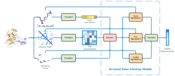
Figure S1: The architecture of the conditional encoder in SidechainDiff

A.2 DiffAffinity network architecture

Given a wild-type $\mathcal{W}$, a mutant $\mathcal{M}$, and their structural contexts of mutations, we first obtain the hidden representations from the pre-trained SidechainDiff, denoted as $h_{\mathrm{wt}}$ and $h_{\mathrm{mt}}$, respectively. We set wild-type and mutant sequences as single features concated with hidden representations from SidechainDiff, distance matrix from wild-type protein structure as pair features, and frames of wild-type protein structure. Then, we input them into IPA transformer encoder [Jumper et al., 2021] to update these hidden representations. A max-pooling layer and an MLP layer follow to predict the final $\Delta\Delta G$. We use the mean squared error (MSE) loss in training.

A.3 Training details for SidechainDiff

For SidechainDiff, we adopt a similar hyperparameter setting of the score-based generative model as used in [Song et al., 2021, De Bortoli et al., 2022]. The diffusion coefficient is parameterized as $g(t)=\sqrt{\beta(t)}$ with $\beta:t\mapsto\beta_{\min}+(\beta_{\max}-\beta_{\min})\cdot t$, where $\beta_{\min}=0.001$ and $\beta_{\max}=2$. To parameterize the vector field on $\mathbb{T}^{4}$, we use a single field per dimension pointing in a consistent direction around the $i^{th}$ component in the product, with the unit norm. Sinusoidal activation functions are utilized.

For the ISM losses $l_{t}^{im}$, we adopt the setting of $\lambda_{t}=g(t)^{2}=\beta_{t}$. All models are trained using the stochastic optimizer Adam with the setting of $\beta_{1}=0.9$ and $\beta_{2}=0.999$ and a batch size of $M$. The learning rate is annealed with a linear ramp from 0 to 1000 and thereafter with a cosine schedule. The total number of iterations, denoted as $N_{\mathrm{iter}}$, is set to 200,000, and we define the batch size $M$ as 32. The reverse diffusion model is configured with 100 steps. The Algorithm 2 illustrates the entire training algorithm.

To sample mutations in training, we mask the rotamers of 10% of the amino acids and introduce noises to the rotamers of amino acids within a $C_{\beta}-C_{\beta}$ distance of $8.0\mathring{A}$ from the closest masked amino acids, simulating the impact of mutations on adjacent amino acids. Following the strategy in RDE [Luo et al., 2023], we add Gaussian noises centered at 0 and its standard deviation depending on the $C_{\beta}-C_{\beta}$ distances.

Algorithm 2 Training Process of SidechainDiff

1:$\epsilon,T,N,\{\mathbf{X}_{0}^{m}\}_{m=1}^{M},\theta_{0},\phi_{0},N_{\mathrm{iter}},P,\{a_{i},\mathbf{R}_{i},\mathbf{x}_{i},\bm{\chi}_{i}\}_{i=1}^{127}$

2:///TRAINING///

3:for $n\in\{0,\dots,N_{\mathrm{iter}}-1\}$ do

4:    $\mathbf{X}_{0}\sim(1/M)\sum_{m=1}^{M}\delta_{X_{0}^{m}}$$\triangleright$ Random mini-batch from dataset

5:    $t\sim U([\epsilon,T])$$\triangleright$ Uinform samping between $\epsilon$ and $T$

6:    $\mathbf{Z}_{t}=\mathrm{Enc}_{\phi_{n}}(\{a_{i},\mathbf{R}_{i},\mathbf{x}_{i},\bm{\chi}_{i}\}_{i=1}^{127})$$\triangleright$ Encode the structural context into hidden representation

7:    $\gamma=t/N$

8:    for $k\in\{0,\dots,N\}$ do $\triangleright$ Approximate forward diffusion with Algorithm 1

9:         $W_{k+1}\sim\mathcal{N}(0,\mathrm{Id})$

10:         $W_{k+1}=\sqrt{\gamma}W_{k+1}$$\triangleright$ the drift coefficient of Algorithm 1 is set as 0 here

11:         $X_{k+1}=\mathrm{exp}_{\mathbf{X}_{0}}(W_{k+1})$

12:    end for

13:    $\mathbf{X}_{t}=X_{N}$

14:    $l_{t}^{\mathrm{im}}(s_{t})=l_{t}^{\mathrm{im}}(s_{\theta_{n}}(\mathbf{X}_{t},t,\mathbf{Z}_{t}))$ $\triangleright$ Compute implicit score matching loss

15:    $\theta_{n+1},\phi_{n+1}=\mathrm{optimizer\_update}(\theta_{n},\phi_{n},l_{t}^{\mathrm{im}}(s_{t}))$ $\triangleright$ ADAM optimizer step

16:end for

17:$\theta^{*}=\theta_{N_{\mathrm{iter}}},\phi^{*}=\phi_{N_{\mathrm{iter}}}$

18:return $\theta^{*},\phi^{*}$

A.4 Baseline models

To benchmark the performance, we train RDE and the two variants of our DiffAffinity (i.e. DiffAffinity* and DiffAffinity-Linear) using the same splits of training and test set with the SKEMPI2 dataset. The implementation details of baseline methods are described below.

DiffAffinity-Linear   DiffAffinity-Linear model represents a simple linear projection of the learned representations from SidechainDiff for the prediction of $\Delta\Delta G$.

DiffAffinity*   In contrast to the original DiffAffinity, no learned representations from SidechainDiff are used in DiffAffinity*. Other settings including model architecture and training procedure are the same with DiffAffinity.

RDE [Luo et al., 2023]   We use the training and testing script in the RDE GitHub repository (https://github.com/luost26/RDE-PPI). And for downstream tasks, we average the predictions from 3 models as the final scores.

Rosetta [Alford et al., 2017]   We use Rosetta version 2023.35 downloaded from the official site (https://www.rosettacommons.org).For a mutated structure, we build its structure using the cartesian_ddg command. $\Delta\Delta G$ is determined by subtracting the energy of the wild-type from that of the mutant predicted by interface_energy.

FoldX [Schymkowitz et al., 2005]   We use FoldX-v5 downloaded from the official site (https://foldxsuite.crg.eu/).For a mutated sequence, we build its structure using the BuildModel command. $\Delta\Delta G$ is determined by subtracting the energy of the wild-type from that of the mutant.

flex ddG [Barlow et al., 2018]   We employed the flex ddG from the GitHub repository found at https://github.com/Kortemme-Lab/flex_ddG_tutorial. The binding affinity was derived using the default setting as outlined in the tutorial.

ESM-1v [Meier et al., 2021]   We use the testing script of ESM-1v in the ESM GitHub repository (https://github.com/facebookresearch/esm). We derive the scores using masked-marginal mode to serve as the metric for $\Delta\Delta G$.

ESM-IF [Hsu et al., 2022]   We failed in running the ESM-IF for the very large complex structures. And in Table 1, we just use results obtained from the published work which benchmarks the performance in the same testing set [Luo et al., 2023].

ESM2 [Lin et al., 2023]    We employ a test script available in the ESM GitHub repository (https://github.com/facebookresearch/esm). The model takes mutant and wild-type sequences as input and produces hidden representations of these sequences using ESM2. The difference between these hidden representations is then passed through a two-layer MLP (Multilayer Perceptron) to predict the change in free energy ($\Delta\Delta G$). Here, we have employed the ESM2 (3B) language model, with the network parameters of the MLP set at $2560\times 64\times 1$. The training was conducted using the Adam optimizer with a learning rate of 5e-4, completing 30,000 training steps.

ESM2* [Lin et al., 2023]    We also utilize the hidden representations from ESM2, similar to the ESM2 model. However, in this case, the hidden representations from the SidechainDiff model are replaced with the hidden representations from ESM2. These modified hidden representations, along with the ESM2 hidden representations, are fed into the DiffAffinity model, which predicts the change in free energy ($\Delta\Delta G$).

DDGPred [Shan et al., 2022]   It’s very challenging to reproduce the training and testing process of DDGPred. First, no training scripts are provided in the DDGPred GitHub repository (https://github.com/HeliXonProtein/binding-ddg-predictor). Second, the model weights provided in the open-source repository are trained on a set that overlaps with the testing set in our work. Thus in Table 1, we just use results obtained from the published work which benchmarks the performance in the same testing set [Luo et al., 2023] and we have not benchmarked the performance of DDGPred in the downstream tasks.

A.5 Dataset of SARS-CoV-2 RBD binding affinity

In the previous study [Starr et al., 2022], 15 crucial mutational sites have been identified that greatly influence SARS-CoV-2 RBD binding affinity. The sites include NE501, SE477, GE339, NE440, TE478, SE373, QE498, EE484, SE371, QE493, GE496, YE505, GE446, SE375, and KE417. We use all 285 possible single-point mutations on these sites to benchmark the performance.

Appendix B B Source code

Code and data are available at https://github.com/EureKaZhu/DiffAffinity/

Appendix C C Additional results of DiffAffinity on the SKEMPI2 dataset

C.1 Performance of DiffAffinity on the SKEMPI2 dataset under different Per-Structure threshold

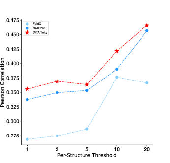
(a)

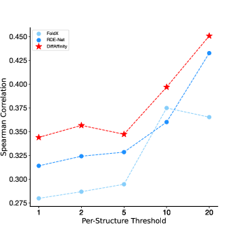
(b)

Figure S2: The performance of Pearson and Spearman correlations across different per-structure filtering thresholds.

To analyze the robustness and accuracy of our performance across different per-structure thresholds, we show the Pearson and Spearman correlation under various per-structure thresholds from $1$ to $20$ (Figure S2a-S2b). DiffAffinity achieves state-of-the-art results compared with other methods under all thresholds.

C.2 Analysis of different pre-training representations

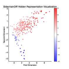
(a)

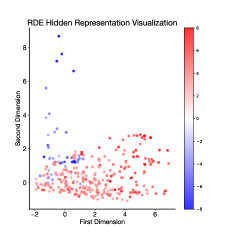
(b)

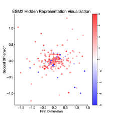
(c)

Figure S3: Visulization of pre-training hidden representations on the SKEMPI2 dataset. We utilize the different colors to represent different $\Delta\Delta G$ obtained by experiment.

To demonstrate the efficacy of the representations learned by SidechainDiff, we performed PCA (Principal Component Analysis) to reduce the dimensions of the obtained representations from SidechainDiff on the SKEMPI2 dataset and visualized the distribution of the representations (Figure S3a).

Furthermore, we have compared several representative methods, including RDE’s representations based on flow models (Figure S3b) and ESM2’s representations based on protein language models (Figure S3c). It can be observed that the representations obtained by SidechainDiff are capable of more effectively distinguishing data under different $\Delta\Delta G$ values. Although ESM2 exhibits outstanding performance in tasks such as protein secondary structure prediction and protein contact recognition, it is insensitive in predicting the effects of mutations on the binding affinity of protein complexes.

C.3 Figures on the performance with the SKEMPI2 dataset

To visually demonstrate the predictive capability of DiffAffinity on the SKEMPI2 dataset, we employed scatter plots and histograms to showcase the statistical properties of results derived from our model DiffAffinity. It is evident that DiffAffinity precisely captures the statistical distribution across the entire SKEMPI2 dataset, including both its single-mutation and multi-mutations subsets (Figure S4).

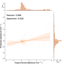
(a)

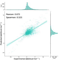
(b)

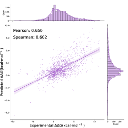
(c)

Figure S4: Results on SKEMPI2 dataset. (a) Correlation between experimental $\Delta\Delta G$s and DiffAffinity predictions on the whole SKEMPI2 dataset. (b) Correlation between experimental $\Delta\Delta G$s and DiffAffinity predictions on the single-mutation subset of SKEMPI2 dataset. (c) Correlation between experimental $\Delta\Delta G$s and DiffAffinity predictions on the multi-mutations subset of SKEMPI2 dataset.

Appendix D D Additional results of SidechainDiff

D.1 Prediction side-chain conformation error with types of amino acids

We show the error of side-chain conformations’ prediction for each amino acid side-chain conformations in the test dataset of PDB-REDO in Table S1. In the majority of amino acids as shown, SidechainDiff surpasses energy-based methods (SCWRL4, Rosseta) and exhibits performance comparable to that of RDE.

Table S1: Mean absolute error of the predicted side-chain torsion angle

Type	$\chi$	SCWRL4	Rosetta	RDE	SidechainDiff
ARG	$1$	$29.30$	$30.50$	$18.92$	$\mathbf{18.60}$
	2	$28.68$	$36.12$	$\mathbf{27.36}$	$33.55$
	3	$57.89$	$60.73$	$\mathbf{51.40}$	$51.73$
	4	$\mathbf{60.35}$	$63.62$	$62.76$	$61.82$
ASN	$1$	$21.70$	$19.39$	$\mathbf{11.30}$	$17.10$
	2	$44.00$	$43.41$	$39.25$	$\mathbf{37.24}$
ASP	$1$	$25.75$	$22.62$	$18.05$	$\mathbf{17.24}$
	2	$23.90$	$21.26$	$\mathbf{20.35}$	$20.95$
CYS	$1$	$24.83$	$25.90$	$16.75$	$\mathbf{7.33}$
GLN	$1$	$33.16$	$31.53$	$26.37$	$\mathbf{26.32}$
	2	$46.33$	$\mathbf{33.96}$	$45.48$	$37.88$
	3	$53.72$	$56.52$	$\mathbf{52.26}$	$60.59$
GLU	$1$	$35.45$	$34.69$	$\mathbf{21.56}$	$35.56$
	2	$38.23$	$38.43$	$\mathbf{36.53}$	$41.75$
	3	$31.50$	$\mathbf{30.85}$	$34.47$	$\mathbf{28.23}$
HIS	$1$	$23.15$	$\mathbf{19.12}$	$29.12$	$25.69$
	2	$70.62$	$61.97$	$74.55$	$\mathbf{54.74}$
ILE	$1$	$13.92$	$14.65$	$10.45$	$\mathbf{7.84}$
	2	$26.43$	$27.54$	$26.84$	$\mathbf{23.29}$

Type	$\chi$	SCWRL4	Rosetta	RDE	SidechainDiff
LEU	$1$	$13.97$	$14.15$	$10.83$	$\mathbf{8.46}$
	2	$23.76$	$27.61$	$24.39$	$\mathbf{21.14}$
LYS	$1$	$31.32$	$33.88$	$30.73$	$\mathbf{24.55}$
	2	$\mathbf{30.95}$	$33.15$	$36.77$	$36.78$
	3	$38.90$	$42.07$	$41.71$	$\mathbf{37.20}$
	4	$51.94$	$53.94$	$54.89$	$\mathbf{51.56}$
MET	$1$	$26.36$	$26.07$	$\mathbf{16.95}$	$25.33$
	2	$38.52$	$36.09$	$\mathbf{29.24}$	$30.15$
	3	$55.11$	$58.77$	$\mathbf{46.33}$	$58.43$
PHE	$1$	$12.30$	$13.08$	$\mathbf{9.64}$	$12.39$
	2	$12.40$	$12.35$	$\mathbf{10.02}$	$11.14$
SER	$1$	$47.19$	$46.83$	$35.48$	$\mathbf{27.51}$
THR	$1$	$28.05$	$22.67$	$\mathbf{13.26}$	$21.09$
TRP	$1$	$\mathbf{14.52}$	$18.64$	$14.69$	$17.29$
	2	$31.74$	$31.44$	$31.39$	$\mathbf{26.01}$
TYR	$1$	$11.39$	$14.56$	$\mathbf{6.83}$	$10.33$
	2	$11.37$	$14.45$	$\mathbf{7.96}$	$8.34$
VAL	$1$	$21.31$	$19.41$	$\mathbf{12.89}$	$15.69$

D.2 Diversity of sampled side-chain conformations

The diversity and prediction accuracy of sampled side-chain conformations from SidechainDiff highly correlates with the structural constraints presented in the protein-protein interface (Table S2). We quantify the diversity using the entropy of the sampled side-chain conformations while utilizing the contact number as a surrogate for the extent of structural constraints. The contact number of an amino acid is defined as the count of neighboring residues within a $C_{\beta}-C_{\beta}$ distance of $8\mathring{A}$. Amino acids with higher contact numbers tend to exhibit greater structural constraints, indicating a more constrained conformation. In highly constrained regions, the sampled side-chain conformations exhibit lower entropy and higher prediction accuracy. These observations align consistently with previous studies in the field [Jones and Thornton, 1996].

Table S2: The diversity of side-chain conformations with different structural constraints

Contact number	Average contact numbers	Average error of $\bm{\chi}$	Entropy
$1\sim 7$	$5.57$	$28.70$	4.10
$8\sim 10$	$8.86$	$22.39$	3.76
$11\sim 19$	$12.36$	$15.43$	3.33

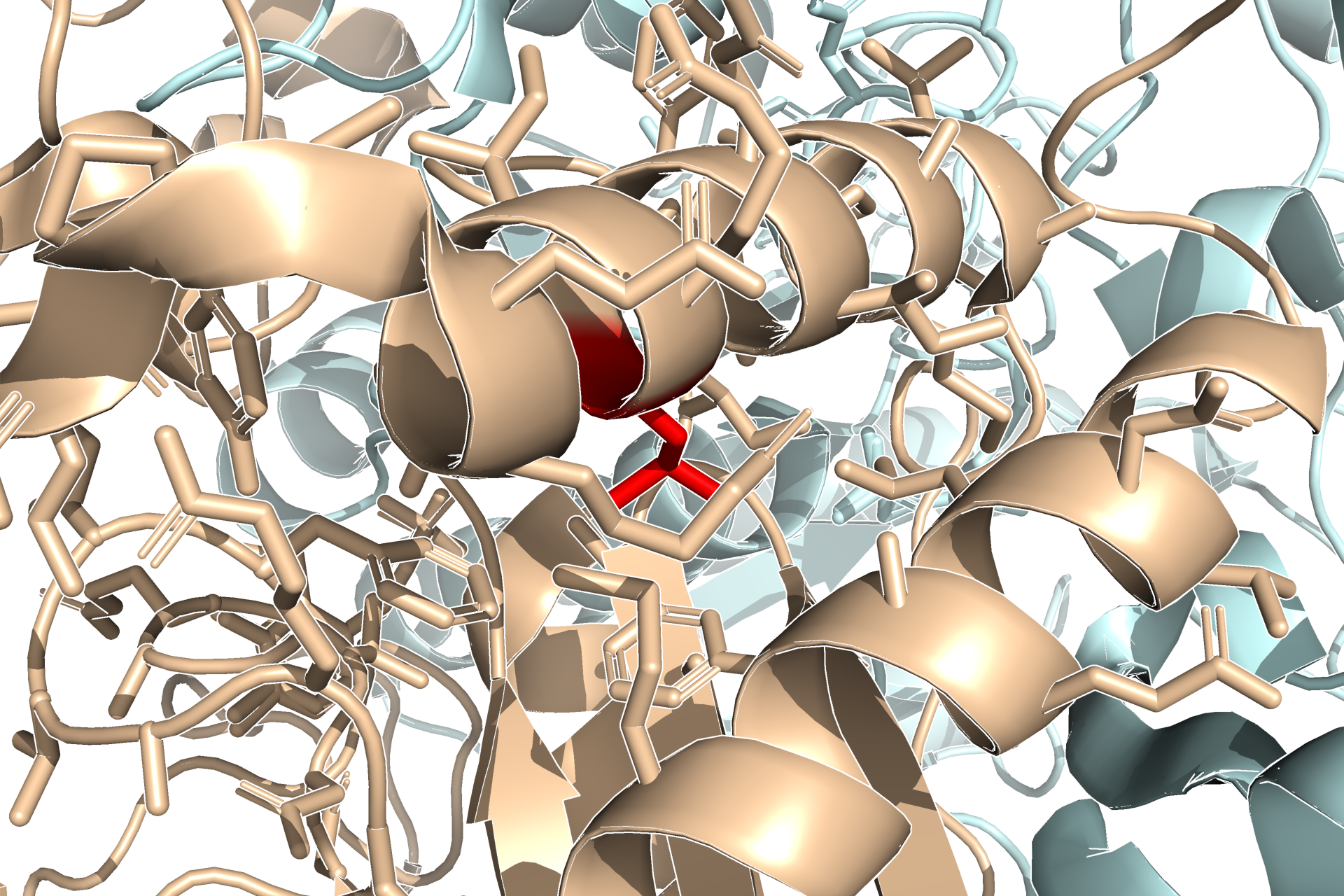
(a)

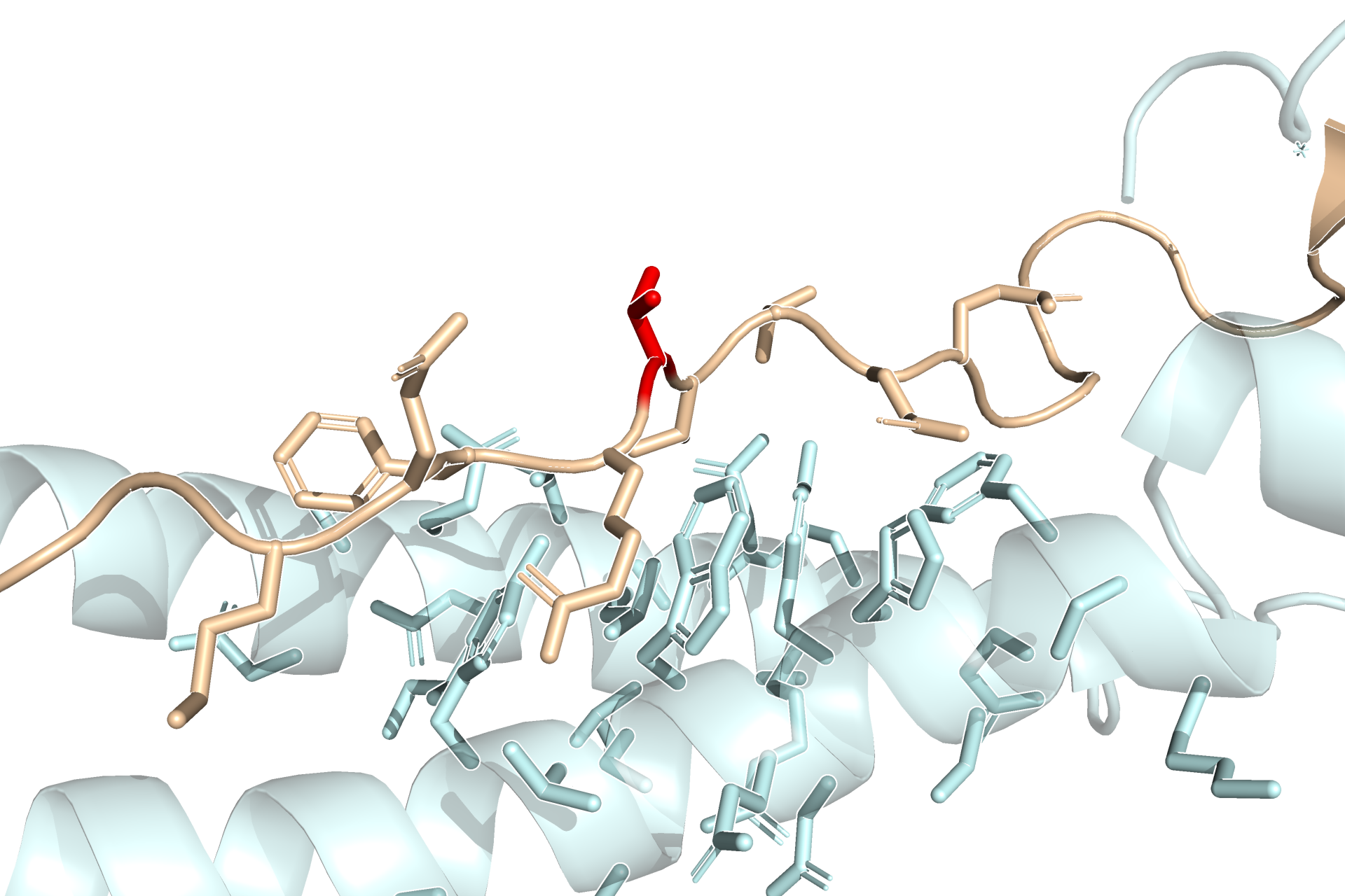
(b)

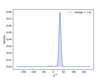
(c)

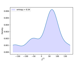
(d)

Figure S5: (a) The structural context of L302 on the chain A of the protein complex 6HBV. (b) The structural context of T28 on the chain D of the protein complex 2P22. (c) The distribution of $\chi^{(1)}$ for the sampled side-chain conformations of L302 on the chain A of the protein complex 6HBV. (d) The distribution of $\chi^{(1)}$ for the sampled side-chain conformations of T28 on the chain D of the protein complex 2P22.

We further present two illustrative cases that highlight the distinction between highly constrained and less constrained regions (Figure S5). The first case involves L302 on the chain A of the protein complex 6HBV (Figure S5a). In this instance, the structural context is characterized by a high degree of constraint, resulting in sampled side-chain conformations with an entropy of 1.67 (Figure S5c). In contrast, the second case focuses on T28, located in the loop region of chain D of the complex 2P22 (Figure S5b). In this scenario, the sampled side-chain conformations display much more flexibility, as indicated by an entropy value of 6.54 (Figure S5d).

Here, we then specify the details that how to calculate the entropy and average error of $\bm{\chi}$ in Table S2. The entropy $S$ is defined by the Boltzmann expression:

$$S=-k_{B}\int p(\mathbf{x})\log p(\mathbf{x})\mathrm{d}\mathbf{x}=-k_{B}\mathbb{E}_{\mathbf{x}\sim p}\log p(\mathbf{x}),$$

where $p(\mathbf{x})$ refers to the distribution of conformation $\mathbf{x}$ and $k_{B}$ denotes the Boltzmann constant. We assign a value of 1 to $k_{B}$ just for simplicity. The entropy $S$ is then calculated as the mean of the log probabilities over 100 samplings.

We calculate the weighted average error of all side-chain torsion angles as follows:

$$\text{Average error of torsion angles}=\frac{1}{N}\sum\limits_{i=1}\limits^{N}\frac{\sum\limits_{j=1}\limits^{4}p(\chi^{(j)})\mathbb{I}_{i}(\chi^{(j)})e_{i}(\chi^{(j)})}{\sum\limits_{j=1}\limits^{4}p(\chi^{(j)})\mathbb{I}_{i}(\chi^{(j)})},$$

where

$$p(\chi^{(j)}) =\frac{1}{N}\sum\limits^{N}\limits_{i=1}\mathbb{I}_{i}(\chi^{(j)}),\quad j=1,2,3,4;$$

$$\mathbb{I}_{i}(\chi^{(j)}) =\begin{cases}1&\text{ ${\rm if}\ \chi^{(j)}\ {\rm exists\ in\ the\ }i{\rm th\ amino\ acid}$}\\ 0&\text{ ${\rm otherwise}$}\end{cases}.$$

Here, $e_{i}(\chi^{(1)})$, $e_{i}(\chi^{(2)})$, $e_{i}(\chi^{(3)})$, and $e_{i}(\chi^{(4)})$ respectively denote the errors of the predicted $\chi^{(1)}$ to $\chi^{(4)}$ in the $i$-th sampling, while $N$ represents the total number of amino acids.

References

- Alford et al. [2017] Rebecca F Alford, Andrew Leaver-Fay, Jeliazko R Jeliazkov, et al. The Rosetta All-Atom Energy Function for Macromolecular Modeling and Design. Journal of Chemical Theory and Computation, 13(6):3031–3048, 2017.
- Arts et al. [2023] Marloes Arts, Victor Garcia Satorras, Chin-Wei Huang, et al. Two for One: Diffusion Models and Force Fields for Coarse-Grained Molecular Dynamics. Journal of Chemical Theory and Computation, 19(18):6151–6159, 2023.
- Baek et al. [2021] Minkyung Baek, Frank DiMaio, Ivan Anishchenko, et al. Accurate prediction of protein structures and interactions using a three-track neural network. Science, 373(6557):871–876, 2021.
- Barlow et al. [2018] Kyle A Barlow, Shane Ó Conchúir, Samuel Thompson, et al. Flex ddG: Rosetta Ensemble-Based Estimation of Changes in Protein-Protein Binding Affinity upon Mutation. The Journal of Physical Chemistry B, 122(21):5389–5399, 2018.
- Calakos et al. [1994] Nicole Calakos, Mark K Bennett, Karen E Peterson, et al. Protein-protein interactions contributing to the specificity of intracellular vesicular trafficking. Science, 263(5150):1146–1149, 1994.
- Corso et al. [2023] Gabriele Corso, Hannes Stärk, Bowen Jing, et al. DiffDock: Diffusion Steps, Twists, and Turns for Molecular Docking. In International Conference on Learning Representations, 2023.
- De Bortoli et al. [2022] Valentin De Bortoli, Emile Mathieu, Michael Hutchinson, et al. Riemannian Score-Based Generative Modelling. In Advances in Neural Information Processing Systems, volume 35, pages 2406–2422, 2022.
- Dhariwal and Nichol [2021] Prafulla Dhariwal and Alexander Nichol. Diffusion models beat gans on image synthesis. In Advances in Neural Information Processing Systems, volume 34, pages 8780–8794, 2021.
- Frazer et al. [2021] Jonathan Frazer, Pascal Notin, Mafalda Dias, et al. Disease variant prediction with deep generative models of evolutionary data. Nature, 599(7883):91–95, 2021.
- Geng et al. [2019] Cunliang Geng, Anna Vangone, Gert E Folkers, et al. iSEE: Interface structure, evolution, and energy-based machine learning predictor of binding affinity changes upon mutations. Proteins: Structure, Function, and Bioinformatics, 87(2):110–119, 2019.
- Ho et al. [2020] Jonathan Ho, Ajay Jain, and Pieter Abbeel. Denoising diffusion probabilistic models. In Advances in Neural Information Processing Systems, volume 33, pages 6840–6851, 2020.
- Hoogeboom et al. [2021] Emiel Hoogeboom, Didrik Nielsen, Priyank Jaini, et al. Argmax Flows and Multinomial Diffusion: Learning Categorical Distributions. In Advances in Neural Information Processing Systems, volume 34, pages 12454–12465, 2021.
- Hopf et al. [2017] Thomas A Hopf, John B Ingraham, Frank J Poelwijk, et al. Mutation effects predicted from sequence co-variation. Nature Biotechnology, 35(2):128–135, 2017.
- Hsu et al. [2022] Chloe Hsu, Robert Verkuil, Jason Liu, et al. Learning inverse folding from millions of predicted structures. In Proceedings of the 39th International Conference on Machine Learning, volume 162, pages 8946–8970, 2022.
- [15] John Ingraham, Max Baranov, Zak Costello, et al. Illuminating protein space with a programmable generative model. bioRxiv. doi:10.1101/2022.12.01.518682.
- Jankauskaitė et al. [2019] Justina Jankauskaitė, Brian Jiménez-García, Justas Dapkūnas, et al. Skempi 2.0: an updated benchmark of changes in protein–protein binding energy, kinetics and thermodynamics upon mutation. Bioinformatics, 35(3):462–469, 2019.
- Jing et al. [2022] Bowen Jing, Gabriele Corso, Jeffrey Chang, et al. Torsional Diffusion for Molecular Conformer Generation. In Advances in Neural Information Processing Systems, volume 35, pages 24240–24253, 2022.
- Jones and Thornton [1996] Susan Jones and Janet M Thornton. Principles of protein-protein interactions. Proceedings of the National Academy of Sciences, 93(1):13–20, 1996.
- Joosten et al. [2014] Robbie P. Joosten, Fei Long, Garib N. Murshudov, et al. The PDB_REDO server for macromolecular structure model optimization. IUCrJ, 1(4):213–220, 2014.
- Jørgensen [1975] Erik Jørgensen. The central limit problem for geodesic random walks. Zeitschrift für Wahrscheinlichkeitstheorie und verwandte Gebiete, 32(1-2):1–64, 1975.
- Jumper et al. [2021] John Jumper, Richard Evans, Alexander Pritzel, et al. Highly accurate protein structure prediction with AlphaFold. Nature, 596(7873):583–589, 2021.
- Kingma et al. [2021] Diederik Kingma, Tim Salimans, Ben Poole, et al. Variational Diffusion Models. In Advances in Neural Information Processing Systems, volume 34, pages 21696–21707, 2021.
- Krivov et al. [2009] Georgii Krivov, Maxim Shapovalov, and Roland Dunbrack. Improved prediction of protein side-chain conformations with SCWRL4. Proteins, 77:778–95, 12 2009.
- Lan et al. [2020] Jun Lan, Jiwan Ge, Jinfang Yu, et al. Structure of the SARS-CoV-2 spike receptor-binding domain bound to the ACE2 receptor. Nature, 581(7807):215–220, 2020.
- Leman et al. [2020] Julia Koehler Leman, Brian D. Weitzner, Steven M. Lewis, et al. Macromolecular modeling and design in Rosetta: recent methods and frameworks. Nature Methods, 17:665–680, 2020.
- Levskaya et al. [2009] Anselm Levskaya, Orion D Weiner, Wendell A Lim, et al. Spatiotemporal control of cell signalling using a light-switchable protein interaction. Nature, 461(7266):997–1001, 2009.
- Li et al. [2016] Minghui Li, Franco L Simonetti, Alexander Goncearenco, et al. Mutabind estimates and interprets the effects of sequence variants on protein–protein interactions. Nucleic Acids Research, 44(W1):W494–W501, 2016.
- Lin et al. [2023] Zeming Lin, Halil Akin, Roshan Rao, et al. Evolutionary-scale prediction of atomic-level protein structure with a language model. Science, 379(6637):1123–1130, 2023.
- Liu et al. [2021] Xianggen Liu, Yunan Luo, Pengyong Li, et al. Deep geometric representations for modeling effects of mutations on protein-protein binding affinity. PLoS Computational Biology, 17(8):e1009284, 2021.
- Luo et al. [2023] Shitong Luo, Yufeng Su, Zuofan Wu, et al. Rotamer Density Estimator is an Unsupervised Learner of the Effect of Mutations on Protein-Protein Interaction. In International Conference on Learning Representations, 2023.
- Mason et al. [2021] Derek M Mason, Simon Friedensohn, Cédric R Weber, et al. Optimization of therapeutic antibodies by predicting antigen specificity from antibody sequence via deep learning. Nature Biomedical Engineering, 5(6):600–612, 2021.
- McPartlon and Xu [2023] Matthew McPartlon and Jinbo Xu. An end-to-end deep learning method for protein side-chain packing and inverse folding. Proceedings of the National Academy of Sciences, 120(23):e2216438120, 2023.
- Meier et al. [2021] Joshua Meier, Roshan Rao, Robert Verkuil, et al. Language models enable zero-shot prediction of the effects of mutations on protein function. In Advances in Neural Information Processing Systems, volume 34, pages 29287–29303, 2021.
- Meireles et al. [2010] Lidio MC Meireles, Alexander S Dï¿ mling, and Carlos J Camacho. ANCHOR: a web server and database for analysis of protein–protein interaction binding pockets for drug discovery. Nucleic Acids Research, 38:W407–W411, 2010.
- Misiura et al. [2022] Mikita Misiura, Raghav Shroff, Ross Thyer, et al. DLPacker: Deep learning for prediction of amino acid side chain conformations in proteins. Proteins: Structure, Function, and Bioinformatics, 90(6):1278–1290, 2022.
- Nichol and Dhariwal [2021] Alexander Quinn Nichol and Prafulla Dhariwal. Improved Denoising Diffusion Probabilistic Models. In Proceedings of the 38th International Conference on Machine Learning, volume 139, pages 8162–8171, 2021.
- Notin et al. [2022] Pascal Notin, Mafalda Dias, Jonathan Frazer, et al. Tranception: Protein Fitness Prediction with Autoregressive Transformers and Inference-time Retrieval. In Proceedings of the 39th International Conference on Machine Learning, volume 162, pages 16990–17017, 2022.
- Papamakarios et al. [2021] George Papamakarios, Eric Nalisnick, Danilo Jimenez Rezende, et al. Normalizing Flows for Probabilistic Modeling and Inference. The Journal of Machine Learning Research, 22(1):2617–2680, 2021.
- Preechakul et al. [2022] Konpat Preechakul, Nattanat Chatthee, Suttisak Wizadwongsa, et al. Diffusion Autoencoders: Toward a Meaningful and Decodable Representation. In Proceedings of the IEEE/CVF Conference on Computer Vision and Pattern Recognition, pages 10619–10629, 2022.
- Riesselman et al. [2018] Adam J Riesselman, John B Ingraham, and Debora S Marks. Deep generative models of genetic variation capture the effects of mutations. Nature Methods, 15(10):816–822, 2018.
- Schwikowski et al. [2000] Benno Schwikowski, Peter Uetz, and Stanley Fields. A network of protein–protein interactions in yeast. Nature Biotechnology, 18(12):1257–1261, 2000.
- Schymkowitz et al. [2005] Joost Schymkowitz, Jesper Borg, Francois Stricher, et al. The FoldX web server: an online force field. Nucleic Acids Research, 33:W382–W388, 2005.
- Shan et al. [2022] Sisi Shan, Shitong Luo, Ziqing Yang, et al. Deep learning guided optimization of human antibody against SARS-CoV-2 variants with broad neutralization. Proceedings of the National Academy of Sciences, 119(11):e2122954119, 2022.
- Sohl-Dickstein et al. [2015] Jascha Sohl-Dickstein, Eric Weiss, Niru Maheswaranathan, et al. Deep Unsupervised Learning using Nonequilibrium Thermodynamics. In Proceedings of the 32nd International Conference on Machine Learning, volume 37, pages 2256–2265, 2015.
- Song et al. [2021] Yang Song, Jascha Sohl-Dickstein, Diederik P Kingma, et al. Score-Based Generative Modeling through Stochastic Differential Equations. In International Conference on Learning Representations, 2021.
- Starr et al. [2022] Tyler N. Starr, Allison J. Greaney, William W. Hannon, et al. Shifting mutational constraints in the SARS-CoV-2 receptor-binding domain during viral evolution. Science, 377(6604):420–424, 2022.
- Steinbrecher et al. [2017] Thomas Steinbrecher, Robert Abel, Anthony Clark, et al. Free Energy Perturbation Calculations of the Thermodynamics of Protein Side-Chain Mutations. Journal of Molecular Biology, 429(7):923–929, 2017.
- T O’Neil and Hoess [1995] Karyn T O’Neil and Ronald H Hoess. Phage display: protein engineering by directed evolution. Current Opinion in Structural Biology, 5(4):443–449, 1995.
- Trippe et al. [2023] Brian L. Trippe, Jason Yim, Doug Tischer, et al. Diffusion Probabilistic Modeling of Protein Backbones in 3D for the motif-scaffolding problem. In International Conference on Learning Representations, 2023.
- Watson et al. [2023] Joseph L Watson, David Juergens, Nathaniel R Bennett, et al. De novo design of protein structure and function with RFdiffusion. Nature, 620(7976):1089–1100, 2023.
- Wu and Li [2023] Fang Wu and Stan Z Li. DIFFMD: A Geometric Diffusion Model for Molecular Dynamics Simulations. In Proceedings of the AAAI Conference on Artificial Intelligence, volume 37, pages 5321–5329, 2023.
- Xu et al. [2022] Gang Xu, Qinghua Wang, and Jianpeng Ma. OPUS-Rota4: a gradient-based protein side-chain modeling framework assisted by deep learning-based predictors. Briefings in Bioinformatics, 23(1):bbab529, 2022.
- Yim et al. [2023] Jason Yim, Brian L. Trippe, Valentin De Bortoli, et al. SE(3) Diffusion Model with Application to Protein Backbone Generation. In Proceedings of the 40th International Conference on Machine Learning, volume 39, page 1672, 2023.
- Zhang et al. [2020] Ning Zhang, Yuting Chen, Haoyu Lu, et al. MutaBind2: Predicting the Impacts of Single and Multiple Mutations on Protein-Protein Interactions. Iscience, 23(3):100939, 2020.
- Zhang et al. [2022] Zijian Zhang, Zhou Zhao, and Zhijie Lin. Unsupervised Representation Learning from Pre-trained Diffusion Probabilistic Models. In Advances in Neural Information Processing Systems, volume 35, pages 22117–22130, 2022.