Core and Halo Properties in Multi-Field Wave Dark Matter

Abstract

In this work, we compute multi-field core and halo properties in wave Dark Matter models. We focus on the case where Dark Matter consists of two light (real) scalars, interacting gravitationally. As in the single-field Ultra Light Dark Matter (ULDM) case, the scalar field behaves as a coherent BEC with a definite ground state (at fixed total mass), often referred to in the literature as a gravitational soliton. We establish an efficient algorithm to find the ground and excited states of such two-field systems. We then use simulations to investigate the gravitational collapse and virialization, starting from different initial conditions, into solitons and surrounding halo. As in the single-field case, a virialized halo forms with a gravitational soliton (ground state) at the center. We find some evidence for an empirical relation between the soliton mass and energy and those of the host halo. We use this to then find a numerical relation between the properties of the two. Finally, we use this to address the issue of alleviating some of the tensions that single-field ULDM has with observational data, in particular, the issue of how a galaxy’s core and radius are related. We find that if galaxies of different masses have similar percentages of the two species, then the core-radius scaling tension is not addressed. However, if the lighter species is more abundant in lighter galaxies, then the tension can be alleviated.

I Introduction

The nature of dark matter remains an important open question. One of the leading candidates for dark matter is a very light boson. For this candidate to make up all the dark matter in the universe, they must have a large number density in the galactic halos. In this case, the particle’s occupancy number can be very large, meaning that the theory can be approximated by classical field theory. These classical fields enjoy wave-like properties, such as interference, etc.

One motivation comes from the idea of ultra-light axions, whose presence can be accommodated in fundamental physics Arvanitaki et al. (2010). In this case, it is plausible that the particles have a mass on the order of $\displaystyle m\sim 10^{-21}\,$eV, or so. Then, the particle’s de Broglie wavelength in a galaxy can be huge. Since typical virial velocities in galaxies are $\displaystyle v\sim 10^{-5}-10^{-3}$ c, the corresponding de Broglie wavelength $\displaystyle\lambda_{dB}\sim h/(mv)$ can be on the order of kpc, or so. Such large de Broglie wavelengths smooth out the centers of galaxies, producing a core rather than a cusp, and can reduce small scale structure generally Hu et al. (2000). For many years this has been suggested as a feature, as some of the simplest simulations of dark matter show a moderately spiky feature near the center, rather than that seen in observations. Whether this so-called “core-cusp problem" is real or not remains a matter of debate. Nevertheless it has historically provided one motivation to consider the phenomenological consequences of ultra-light bosonic dark matter. Furthermore, the idea of ultra-light bosons as dark matter is interesting in its own right as it provides new wave-phenomenology, such as interference patterns, not present in standard (heavy) dark matter models.

Despite these interesting motivations, in the last few years, observational constraints on single component Ultra Light Dark Matter (ULDM) have become more and more severe Dalal and Kravtsov (2022); Irš ič et al. (2017); Armengaud et al. (2017); Chan et al. (2022); Powell et al. (2023); Hertzberg and Loeb (2023). There is therefore increasing interest in opening up more parameter space in the ULDM picture by adding more light scalars to the model Huang et al. (2023); Luu et al. (2023); Gosenca et al. (2023); Glennon et al. (2023); Jain et al. (2023); Eby et al. (2020); Amin et al. (2022). For example, this can suppress the heating of stars near cores, suppressing the effect mentioned in Ref. Dalal and Kravtsov (2022). Moreover, multiple light scalars is often argued as more natural from the point of view of fundamental physics (e.g., Arvanitaki et al. (2010)).

In this work, we will pay particular attention to another apparent tension that exists between single component ULDM and observational data; there are hints from data on galaxies (e.g., see Ref. Rodrigues et al. (2017)) that the size of the galactic core $\displaystyle R_{c}$ and the corresponding density $\displaystyle\rho_{c}$ obey an approximate scaling relation $\displaystyle\rho_{c}\propto 1/R_{c}^{\beta}$, with $\displaystyle\beta\sim 1$ (in fact the value $\displaystyle\beta\approx 1.3$ is a best fit value to a set of galaxies. However, in Ref. Deng et al. (2018) it was shown that this scaling relation is not compatible with any single-field bosonic model. In the simple Newtonian gravity dominated regime, the single-field bosonic model predicts a relation $\displaystyle\rho\propto 1/R_{c}^{\beta}$ with $\displaystyle\beta=4$. Furthermore, Ref. Deng et al. (2018) showed that if a self-interacting potential $\displaystyle V$ is included, it was shown that there is no choice that leads to the observed scaling with stable solutions.

In Ref. Guo et al. (2021), it was suggested that a two-field bosonic model may help the situation. Here it is explained that the space of solutions is increased, leading to a larger array of possibilities than the precise $\displaystyle\rho_{c}\propto 1/R_{c}^{4}$ prediction of the single field model in the Newtonian gravity dominated regime.

In this work, we wish to improve upon this work on multi-field models in several ways: (i) we will calculate the space of solitonic solutions more carefully, (ii) we introduce a prescription that allows one to automate the solitonic solution for multi-field models, (iii) we run simulations (albeit within a spherically symmetric restriction) to obtain scaling relations, (iv) we learn the trends of the space of solitons that naturally arise from different kinds of initial conditions, (v) we lay out the requirements in how the relative fraction of fields must occupy different galaxies in order to better explain the data, or else, to falsify the proposal.

Our paper is organized as follows: In Section II we start with the relativistic theory of two-scalar fields, and take the nonrelativistic limit, and describe the basic solitonic (static) solutions. In Section III we formulate a numerical dynamical treatment, from different choices of initial conditions, to determine which types of solitons emerge. We obtain some empirical scaling relations from these results, albeit the validity of this scaling needs to be subjected to larger scrutiny in future work. In Section IV we present possible cosmological implications of these results, through establishing a multi-field relation between the soliton’s properties and the halo mass. In Section V we conclude and discuss our findings. Finally, in the Appendix, we provide more details of the solitons.

II The Schrödinger-Poisson system

We consider two scalar fields minimally coupled to gravity with action (signature -+++, units $\displaystyle\hbar=c=1$):

$$S=\int d^{4}x\sqrt{-g}\left[\frac{\mathcal{R}}{16\pi G}+\mathcal{L_{M}}\right]$$ (1)

Where the matter contribution to the action is provided by two massive (real) scalars

$$\mathcal{L_{M}}=-\frac{1}{2}\partial_{\mu}\phi_{1}\partial^{\mu}\phi_{1}-\frac{1}{2}\partial_{\mu}\phi_{2}\partial^{\mu}\phi_{2}-\frac{1}{2}m_{1}^{2}\phi_{1}^{2}-\frac{1}{2}m_{2}^{2}\phi_{2}^{2}$$ (2)

Where $\displaystyle m_{1}$ and $\displaystyle m_{2}$ are the masses of $\displaystyle\phi_{1}$ and $\displaystyle\phi_{2}$ respectively. We can also add higher order nonlinear terms in a potential, but this is the leading-order terms for any two-scalar system. Terms proportional to higher powers of $\displaystyle\phi$ are in general also present, in particular if the scalar under consideration is an axion-like particle, self-interactions should be present from a cosine-like potential. However, in the current work we will assume to be in a regime where we can safely neglect those terms and focus on the dynamics of the system given in Eqs. (1) and (2). Since we are concerned with Dark Matter, we can assume the typical velocities of the scalar particles to be of order $\displaystyle v\sim 10^{-5}-10^{-3}c$, which is the typical velocities of particles in a galactic halo (from dwarfs to large galaxies). Therefore, we can safely move to the non-relativistic regime, in which we treat gravity in the Newtonian limit.

II.1 The Non-Relativistic Limit of Scalar Fields

The non-relativistic limit of the action in Eq. (1) has been extensively discussed in the literature. We present a brief derivation here. The basic procedure is to decompose each real scalar in a sum of complex degrees of freedom, after factorizing out its primary oscillations in an $\displaystyle e^{-imt}$ factor, as follows

$$\displaystyle\phi_{1}=\frac{1}{\sqrt{2m_{1}}}\left(\psi(\vec{x},t)e^{-im_{1}t}+c.c.\right)$$ (3)

$$\displaystyle\phi_{2}=\frac{1}{\sqrt{2m_{2}}}\left(\chi(\vec{x},t)e^{-im_{2}t}+c.c.\right)$$ (4)

The non-relativistic limit then corresponds to assuming that the complex degrees of freedom $\displaystyle\psi$ and $\displaystyle\chi$ are slowly varying in space and time. Relatedly, we preserve the degrees of freedom by building an action that involves only one derivative acting on $\displaystyle\psi,\,\chi$, rather than the two derivatives acting on $\displaystyle\phi_{1},\,\phi_{2}$. We are in the limit where $\displaystyle|\nabla\psi|\ll m_{1}|\psi|$ and $\displaystyle|\dot{\psi}|\ll m_{1}|\psi|$. Similarly $\displaystyle|\nabla\chi|\ll m_{2}|\chi|$ and $\displaystyle|\dot{\chi}|\ll m_{2}|\chi|$. Lastly, we assume to be in a weak field limit where $\displaystyle\frac{|\psi|}{\sqrt{m_{1}}M_{Pl}}\sim\frac{|\chi|}{\sqrt{m_{1}}M_{Pl}}\ll 1$ ($\displaystyle M_{Pl}=1/\sqrt{G}$). In this limit, gravity becomes Newtonian, with the only relevant term in the metric being $\displaystyle g_{tt}=-1-2U$, where $\displaystyle U$ is the gravitational potential. The Lagrangian density then becomes (to lowest dynamical order)

$$\displaystyle\mathcal{L}_{nr} \displaystyle= \displaystyle-\frac{\nabla U\nabla U}{8\pi G}-\frac{1}{2m_{1}}\nabla\psi\nabla\psi^{*}-\frac{1}{2m_{2}}\nabla\chi\nabla\chi^{*}-U\left(m_{1}|\psi|^{2}+m_{2}|\chi|^{2}\right)$$ (5)

$$\displaystyle+\frac{i}{2}\left(\dot{\psi}\psi^{*}-\dot{\psi^{*}}\psi\right)+\frac{i}{2}\left(\dot{\chi}\chi^{*}-\dot{\chi^{*}}\chi\right)$$

Interestingly, in this non-relativistic limit, there is an accidental pair of $\displaystyle U(1)$ global symmetries in Eq. (5) (the action is invariant under a change of the field’s phase). So the system contains two conserved quantities $\displaystyle N_{1}=\int d^{3}x\,n_{1}(\vec{x},t)$ and $\displaystyle N_{2}=\int d^{3}x\,n_{2}(\vec{x},t)$, with corresponding number densities $\displaystyle n_{1}(\vec{x},t)=|\psi|^{2}$ and $\displaystyle n_{2}(\vec{x},t)=|\chi|^{2}$. These are just the number densities of the particles of the two respective species (the mass density is then given by $\displaystyle\rho_{i}(\vec{x})=m_{i}n_{i}(\vec{x})$), which is conserved in the non-relativistic regime as particle number changing processes are relativistic and suppressed.

The expressions for the masses and energies in each field are

$$M_{\psi}=\int d^{3}x\,m_{1}|\psi|^{2}\quad\textrm{and}\quad M_{\chi}=\int d^{3}x\,m_{2}|\chi|^{2}$$ (6)

$$K_{\psi}=\int d^{3}x\,\frac{1}{2m_{1}}\nabla\psi\nabla\psi^{*}\quad\textrm{and}\quad K_{\chi}=\int d^{3}x\,\frac{1}{2m_{2}}\nabla\chi\nabla\chi^{*}$$ (7)

$$W_{\psi}=\int d^{3}x\,\frac{m_{1}U}{2}|\psi|^{2}\quad\textrm{and}\quad W_{\chi}=\int d^{3}x\,\frac{m_{2}U}{2}|\chi|^{2}$$ (8)

With $\displaystyle M_{i}$, $\displaystyle K_{i}$ and $\displaystyle W_{i}$ the mass, kinetic and gravitational energy of each field respectively. The total energy of the system is given by (neglecting the rest mass energy which always dominates in the NR-regime)

$$E_{tot}=K_{\psi}+K_{\chi}+W_{\psi}+W_{\chi}$$ (9)

By varying the above action, the dynamics are described by the well-known Schrödinger-Poisson system of equations

$$\displaystyle i\dot{\psi} \displaystyle= \displaystyle-\frac{\nabla^{2}}{2m_{1}}\psi+m_{1}U\psi$$ (10)

$$\displaystyle i\dot{\chi} \displaystyle= \displaystyle-\frac{\nabla^{2}}{2m_{2}}\chi+m_{2}U\chi$$ (11)

where the gravitational potential $\displaystyle U$ is the solution to the Poisson equation

$$\nabla^{2}U=4\pi G\left(m_{1}|\psi|^{2}+m_{2}|\chi|^{2}\right)$$ (12)

This set of equations will form the basis of our study, which to first order, should describe the dynamics of scalar dark matter particles on galactic scales. Since we will exploit it later, we note that there is a scale transformation that leaves this set of equations invariant. In particular,

$$\psi(\vec{x},t)\rightarrow\lambda^{2}\,\psi(\lambda\vec{x},\lambda^{2}t)$$ (13)

$$\chi(\vec{x},t)\rightarrow\lambda^{2}\,\chi(\lambda\vec{x},\lambda^{2}t)$$ (14)

$$U(\vec{x})\rightarrow\lambda^{2}\,U(\lambda\vec{x})$$ (15)

Where in Eq. (15) we suppress the dependence of $\displaystyle U$ on $\displaystyle t$ as the gravitational potential is itself nondynamical, and purely sourced by the presence of the scalar fields.

Eqs. (10) (11) and (12) describe the behavior of a coherent Bose-Einstein condensate, with conserved particle numbers $\displaystyle N_{1}$ and $\displaystyle N_{2}$. To understand the dynamics of the system, it is therefore quintessential to find its static solutions at fixed particle number, akin to the eigenstates of the Hamiltonian in quantum mechanics.

II.2 Static Solutions

The static solutions of the Schrödinger-Poisson system are those solutions whose gravitational potential remains constant over time. Therefore the time-dependence of the scalar has to be a pure space-independent phase. In particular, one can look for solutions of the form

$$\psi(\vec{x},t)=\left(\frac{\sqrt{m_{1}}M_{Pl}}{\sqrt{4\pi}}\right)\Psi(r)e^{-i\gamma m_{1}t}$$ (16)

$$\chi(\vec{x},t)=\left(\frac{\sqrt{m_{1}}M_{Pl}}{\sqrt{4\pi}}\right)\Phi(r)e^{-i\kappa m_{2}t}$$ (17)

Where $\displaystyle\gamma$ and $\displaystyle\kappa$ are chemical potentials for each of the species. We limit our search to spherical solutions, as those are the ones that generally will minimize the energy of the configuration. We can take the radial profiles, $\displaystyle\Psi$ and $\displaystyle\Phi$, to be real functions without loss of generality.

The problem is thus reduced to solving the eigenvalue problem characterized by the following set of equations, where we introduced dimensionless variables through $\displaystyle\tilde{x}_{\mu}=m_{1}x_{\mu}$

$$\displaystyle\nabla^{2}\Psi \displaystyle= \displaystyle 2\left(U-\gamma\right)\Psi$$ (18)

$$\displaystyle\nabla^{2}\Phi \displaystyle= \displaystyle 2\left(\frac{m_{2}}{m_{1}}\right)^{2}\left(U-\kappa\right)\Phi$$ (19)

with the gravitational Poisson equation

$$\nabla^{2}U=\left(\Psi^{2}+\frac{m_{2}}{m_{1}}\Phi^{2}\right)$$ (20)

where in spherical symmetry the Laplacian is

$$\nabla^{2}=\partial^{2}_{r}+\frac{2}{r}\partial_{r}$$ (21)

We are looking for localized solutions of the above set of equations. We first fix the central amplitude of the fields to $\displaystyle\Psi(0)=\Psi_{0}$ and $\displaystyle\Phi(0)=\Phi_{0}$. Next, imposing the regularity conditions $\displaystyle\partial_{r}\Psi(0)=\partial_{r}\Phi(0)=\partial_{r}U(0)=0$, the system can effectively be solved through a two-parameter shooting method. The ground state solutions are those in which the fields have no nodes, and monotonically approach zero at large $\displaystyle r$.

II.3 Iterative Procedure

In the single field case, there is only one chemical potential and the shooting method is rather straightforward (work on the single field case includes Refs. Chavanis (2011); Chavanis and Delfini (2011); Schiappacasse and Hertzberg (2018); Visinelli et al. (2018)). However, we found that it’s difficult to find the localized solution, while shooting the two parameters $\displaystyle\gamma$ and $\displaystyle\kappa$ simultaneously. We thus employ an iterative method which we found to converge efficiently. First, we split the gravitational potential into two parts, $\displaystyle U(r)=U_{\Psi}(r)+U_{\Phi}(r)$, where

$$\displaystyle\nabla^{2}U_{\Psi}=\Psi^{2}$$ (22)

$$\displaystyle\nabla^{2}U_{\Phi}=\frac{m_{2}}{m_{1}}\Phi^{2}$$ (23)

The iterative method can then be summarized as

1. Initially, set $\displaystyle U_{\Phi}=0$ and find the localized solution of the system

   $$\nabla^{2}\Psi=2\left(U_{\Psi}+U_{\Phi}-\gamma\right)\Psi$$ (24)

   $$\nabla^{2}U_{\Psi}=\Psi^{2}$$ (25)

   (even though in this very first step $\displaystyle U_{\Phi}=0$, we formally include it in the first equation here, as this will be important when we repeat the procedure, which will involve a nonzero $\displaystyle U_{\Phi}$). This system can be solved straightforwardly using shooting methods familiar from the single field case as it involves only one parameter $\displaystyle\gamma$.

2. Updating the solution of $\displaystyle U_{\Psi}$ obtained from step 1, find the localized solution of the system

   $$\nabla^{2}\Phi=2\left(\frac{m_{2}}{m_{1}}\right)^{2}\left(U_{\Psi}+U_{\Phi}-\kappa\right)\Phi$$ (26)

   $$\nabla^{2}U_{\Phi}=\frac{m_{2}}{m_{1}}\Phi^{2}$$ (27)

   Again, there is no difficulty in finding the localized solutions of this system as it involves only one parameter $\displaystyle\kappa$.

3. Iterate through steps 1 and 2, making sure to update the gravitational potentials at each step until convergence of the solutions is reached.

In practice, we find that this method converges after $\displaystyle\mathcal{O}(10)$ iterations. Note that this method can straightforwardly be extended to include non-gravitational interactions between the scalars, such as quartic interactions. However, for realistic models, such interactions are normally negligible, and in any case, is beyond the scope of the current work.

At fixed central density $\displaystyle\Psi_{0}$ and $\displaystyle\Phi_{0}$, there are an enumerable infinite amount of solutions labeled by $\displaystyle n_{1}$ and $\displaystyle n_{2}$, indicating the number of nodes in $\displaystyle\Psi$ and $\displaystyle\Phi$ respectively. To find any particular solution we have to solve for $\displaystyle\Psi$ and $\displaystyle\Phi$ with the appropriate number of nodes through each iteration. In the remainder of this work, we will focus on the ground state (no nodes) configurations with $\displaystyle n_{1}=n_{2}=0$, as it is expected that those are the gravitational solitons that form at the center of galaxies. We are thus able to find the static ground state solutions of the Schrödinger-Poisson system of equations at fixed central densities $\displaystyle\Psi_{0}$, $\displaystyle\Phi_{0}$.

The scaling relations of Eqs. (13), (14) and (15) then allow us to find any solution that has the same ratio of central densities $\displaystyle f=\frac{\Phi_{0}}{\Psi_{0}}$, as this ratio is conserved through the transformation. Therefore, it is only necessary to find the ground state soliton once for each ratio of central densities, noting also that if the ratio is extreme, the ground state effectively becomes the single-field soliton. The properties of the different solutions are related to each other via

$$\displaystyle M_{\Psi,f,\lambda}=\lambda M_{\Psi,f,0}\quad\textrm{and}\quad M_{\Phi,f,\lambda}=\lambda M_{\Phi,f,0}$$ (28)

$$\displaystyle K_{\Psi,f,\lambda}=\lambda^{3}K_{\Psi,f,0}\quad\textrm{and}\quad K_{\Phi,f,\lambda}=\lambda^{3}K_{\Phi,f,0}$$ (29)

$$\displaystyle W_{\Psi,f,\lambda}=\lambda^{3}W_{\Psi,f,0}\quad\textrm{and}\quad W_{\Phi,f,\lambda}=\lambda^{3}W_{\Phi,f,0}$$ (30)

Where the subscript $\displaystyle f,0$ corresponds to a reference value at each ratio $\displaystyle f$. In what follows we will take the reference solutions to be the solutions where $\displaystyle\Psi_{0}=1$ and $\displaystyle\Phi_{0}=f$.

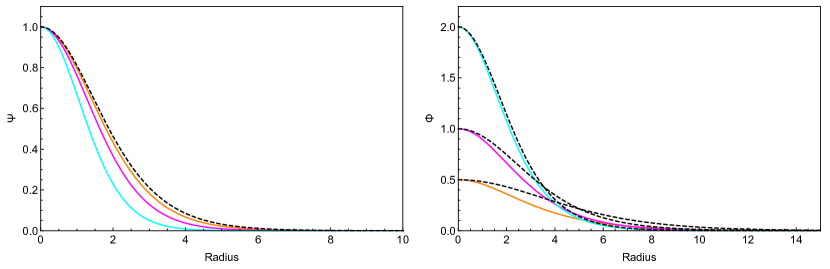
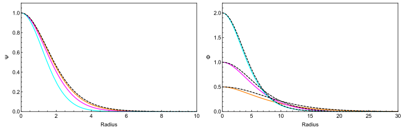
Figure 1: Top panel: Some ground state soliton solutions in the case where $\displaystyle m_{2}/m_{1}=1/2$. Bottom panel: Some ground state soliton solutions in the case where $\displaystyle m_{2}/m_{1}=1/5$. Here we plot three cases: one where the heavier field dominates the mass contribution (orange), an intermediate case (magenta), and a case where the light field dominates (cyan). The black dashed line corresponds to the single-field solution which matches best in the case where one of the two fields dominates the total mass of the solution. Left: The field profile of the heavy field $\displaystyle\Psi(r)$. Right: The field profile of the light field $\displaystyle\Phi(r)$

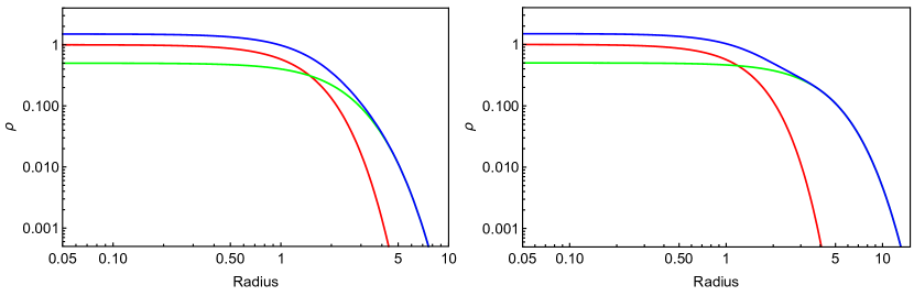
Figure 2: The mass density profile for a typical ground state soliton solution. We plot the mass density $\displaystyle\rho$ for the heavy field (red), light field (green), and the total sum (blue). The nested nature of the soliton is clearly visible, where initially the heavy field dominates the total density near the center. However, due to the larger De Broglie wavelength of the lighter field, there exists a "turnover point" where the light field starts to dominate. Left: $\displaystyle m_{2}/m_{1}=1/2$. Right: $\displaystyle m_{2}/m_{1}=1/5$.

II.4 Sample Solutions

In Fig. 1 top panel and bottom panel, we show some ground state solitons with $\displaystyle m_{2}/m_{1}=1/2$ and $\displaystyle m_{2}/m_{1}=1/5$ respectively. We see that there is nontrivial behavior. In particular, the cyan curve crosses the magenta and orange curves for the second field $\displaystyle\Phi(r)$. We can understand this as follows: The cyan curve for $\displaystyle\Phi$ is so high (for small $\displaystyle r$) that it carries a large amount of mass. This means the fields are concentrated around this heavy center. However, as we lower the central value in $\displaystyle\Phi$ to the magenta or orange curve, the mass is reduced, the gravitational pull is reduced, and the fields are more spread out. In Fig. 2 we plot the mass density profiles for a solution with a comparable total mass. The larger De Broglie wavelength of the light field is clearly visible, resulting in an interesting density profile, that is initially dominated by the heavy field, and then gets dominated by the lighter field.

Given that indeed these static solutions of the Schrödinger-Poisson system exist, we can investigate their dynamics. In particular, are the solutions that we found actually stable? Second, do they form dynamically under generic conditions? We address the first point in Appendix A, and the second will be the main concern of the next section.

III Dynamical Evolution, Virialization & Halo Formation

It is well known that single-field ULDM dynamically forms virialized Dark Matter halos with an approximately constant density core and an NFW-like tail. The core can be thought of as a highly populated ground state soliton, similar to those found in section II.2. The ULDM halos that form in (cosmological) simulations have been argued to match observations of rotation curves better than standard CDM by suppressing small-scale structure. Some of the relevant issues are Core vs. Cusp, Missing Satellite, and Too Big To Fail Problems. It’s important to check that multi-field ULDM still forms halos with these properties, as there would be no reason to consider them if they do not.

In this section, we study the dynamics of multi-field ULDM enforcing spherical symmetry, by performing simulations of the virialization of a cloud of two-field ULDM. We acknowledge the limitations of enforcing spherical symmetry. However, as we’ll show, our results are highly suggestive and provide enough evidence to make cosmological extrapolations.

III.1 Numerical Experiments

We are interested in answering two questions concerning the multi-field Schrödinger Poisson system of equations. Firstly, is the system able to virialize from generic initial conditions, forming a cored solitonic center with an NFW tail? Then if this does indeed happen, can we identify a relationship between the properties of the soliton core and the halo as a whole? In Schive et al. (2014a, b) the relation between the core and halo masses in single-field ULDM was first discussed. It has since then been discussed in numerous works. We are interested in whether similar dependencies exist in the multi-field system.

To study these questions we perform numerical simulations of the Schrödinger Poisson system of Eqs. (10),(11) and (12) with an Runge-Kutta-4 integrator for time integration. At each time step, we solve the Poisson equation with and sixth-order accurate ODE solver. We use the following change of variables to obtain a dimensionless set of equations

$$\tilde{x}^{\mu}=m_{1}x^{\mu}\quad\textrm{;}\quad\tilde{\psi}=\left(\frac{\sqrt{4\pi}}{\sqrt{m_{1}}M_{pl}}\right)\psi\quad\textrm{;}\quad\tilde{\chi}=\left(\frac{\sqrt{4\pi}}{\sqrt{m_{1}}M_{pl}}\right)\chi$$ (31)

Where tildes refer to dimensionless quantities. The SP-equations then become

$$i\dot{\tilde{\psi}}=-\frac{\nabla^{2}}{2}\tilde{\psi}+U\tilde{\psi}$$ (32)

$$i\dot{\tilde{\chi}}=-\frac{m_{1}\nabla^{2}}{2m_{2}}\tilde{\chi}+\frac{m_{2}}{m_{1}}U\tilde{\chi}$$ (33)

$$\nabla^{2}U=\left(|\tilde{\psi}|^{2}+\frac{m_{2}}{m_{1}}|\tilde{\chi}|^{2}\right)$$ (34)

It is also noteworthy that under this change of variables we get natural definitions of dimensionless masses and energy related to dimensionful quantities as $\displaystyle\tilde{M}=\ \left(m_{1}/M_{pl}^{2}\right)M$ and $\displaystyle\tilde{E}=\left(m_{1}/M_{pl}^{2}\right)E$. Eqs. (32), (33) and (34) only explicitly depends on $\displaystyle m_{1}/m_{2}$. As long as the non-relativistic description of the scalars is valid, the overall dynamics thus only depend on the ratio of fundamental masses. In what follows we drop the tilde and work with dimensionless quantities unless explicitly stated. We investigate the virialization starting from two distinct types of initial conditions.

1. Gaussian field profiles parameterized by

   $$\psi(r,0)=\left(\frac{16M_{\psi}^{2}}{\pi R_{\psi}^{6}}\right)^{\frac{1}{4}}e^{-\frac{1}{2}\left(\frac{r}{R_{\psi}}\right)^{2}}$$ (35)

   $$\chi(r,0)=\left(\frac{16m_{1}^{2}M_{\chi}^{2}}{\pi m_{2}^{2}R_{\chi}^{6}}\right)^{\frac{1}{4}}e^{-\frac{1}{2}\left(\frac{r}{R_{\chi}}\right)^{2}}$$ (36)

   Where $\displaystyle M_{\psi}$, $\displaystyle M_{\chi}$, $\displaystyle R_{\psi}$ and $\displaystyle R_{\chi}$ are free parameters. Note that the phase of the complex fields is 0 everywhere initially. The fields are thus identically real at $\displaystyle t=0$.

2. Random initialization of a gas of particles with specific velocity dispersion. Specifically, we initialize in Fourier space with,

   $$\psi(|k|,0)=\psi_{k,re}+\psi_{k,im}i$$ (37)

   $$\chi(|k|,0)=\chi_{k,re}+\chi_{k,im}i$$ (38)

   Where the different coefficients of $\displaystyle\psi_{k}$ and $\displaystyle\chi_{k}$ are taken as Gaussian variables with variance given by $\displaystyle\sigma_{\psi}^{2}=2^{\frac{7}{2}}\pi^{\frac{5}{2}}M_{\psi}e^{-\frac{k^{2}}{2}}$ and $\displaystyle\sigma_{\chi}^{2}=2^{\frac{7}{2}}\pi^{\frac{5}{2}}\left(\frac{m_{1}}{m_{2}}\right)^{4}M_{\chi}e^{-\frac{m_{1}^{2}k^{2}}{2m_{2}^{2}}}$. Once all the coefficients are determined we perform an inverse Fourier transform to obtain the initial conditions in real space. This initialization will more closely model the randomness to be expected of an over-density of Dark Matter before collapsing. However, we noted that they generally take longer to collapse, and the Gaussian profile is still valuable in terms of computational efficiency.

For both type of initial conditions, we have another requirement on the parameters that we use to set the initial field profiles. Namely, we require the system to be bounded at the initial time; thus the total energy is smaller than $\displaystyle 0$. Finally, it is important to note that not necessarily all particles in our initial conditions will tend to collapse and produce a virialized halo. Some will tend to leave the gravitationally bounded domain towards infinity. As we only possess finite computational power, we accommodate this by defining a physical box in which we measure properties of the halo, surrounded by an absorbing boundary layer, in which escaped particles can decay. To be explicit, we follow the procedure outlined in Guzmá n and Ureña-López (2004). Having discussed our numerical setup, we now move on to our results.

III.2 Empirical Findings

The virial theorem states that $\displaystyle E_{kin}=\frac{1}{2}|E_{grav}|$ for a stable gravitationally bound system. In our setup, we are thus interested in configurations that obey

$$\frac{K}{|W|}=\frac{K_{\psi}+K_{\chi}}{|W_{\psi}+W_{\chi}|}=\frac{1}{2}$$ (39)

within our numerical domain. It is not obvious that the virial theorem applies to ULDM halos. An elegant proof of this is given in Hui et al. (2017), which is easily generalizable to multi-field systems. In our simulations, we found that, regardless of initialization, the system virializes. We show the evolution of the virial coefficient $\displaystyle K/|W|$ in Fig. 3. In practice, we evolve from our initial conditions until sufficient time has passed for the system to virialize and become approximately static. We then take measurements of this “model” halo which has formed in our numerical domain.

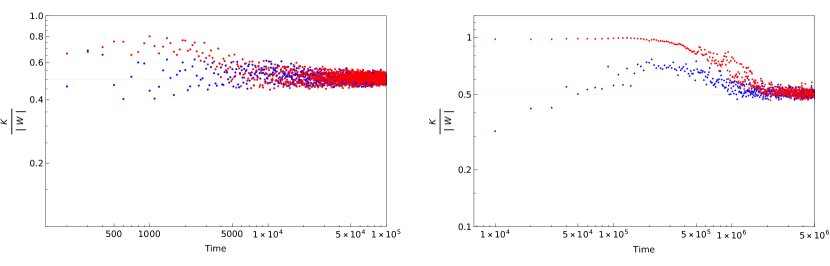
Figure 3: Typical evolution of the virial coefficient $\displaystyle K/|W|$ for undercooled (meaning $\displaystyle K/|W|<0.5$ initially) (blue) and overcooled (meaning $\displaystyle K/|W|>0.5$ initially) (red) initial conditions. Although the undercooled situation oscillates around $\displaystyle 0.5$ earlier, eventually both situations tend to virialization, in a sense carrying no memory of the initial conditions. Left: Initialization from a Gaussian packet following Eqs. (35) and (36). Right: Initialization from random initial conditions following Eqs. (37) and (38). A Gaussian initialization takes about one order of magnitude less time to form a virialized configuration and hence offer large computational benefits.

III.2.1 The formation of the halo

Regardless of initial conditions, eventually, a regime is reached where condition (39) is obeyed. We show this for some typical initial conditions in Fig. 3. The remaining gravitationally bound structure can be seen as a model Dark Matter halo (or Boson star) supported by “Quantum” pressure. Virialization happens through a combination of gravitational collapse and the ejection of fast-moving matter to the absorbing boundary layer. In this work, we do not make statements about the precise timescales involved in these processes. However, we note that virialization proceeds more efficiently in the case where the initial conditions are “undercooled” ($\displaystyle k/|W|<1/2$) as opposed to “overcooled” ($\displaystyle k/|W|>1/2$). In the latter case, our setup tends to eject more matter into the absorbing layer, requiring more time. Understanding all the timescales involved in condensing into a two-field bound halo, is a very important endeavor, but beyond the scope of this work. We plan to address these questions in the future with more representative 3D simulations. In Figs. 4 and 5 we show the process of virialization for typical cases of each type of initialization highlighted in the previous section. For these simulations, we took two benchmark mass ratios of $\displaystyle m_{2}/m_{1}=1/2$ and $\displaystyle m_{2}/m_{1}=1/5$.

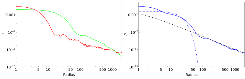
Figure 4: The (spherical) gravitational collapse of our two-field system, starting from a Gaussian packet following Eqs. (35) and (36) with $\displaystyle m_{2}/m_{1}=1/5$. Left: The time-averaged number density profiles of the heavy (red) and light (green) fields. We see that the fields form a cored halo with a decaying tail. The decaying tail is not exactly NFW although it clearly follows some power law. Right: The initial (dashed) and final time-averaged (full) mass density profiles. The tail of the full mass density profile follows NFW almost exactly (black dashed line). The nested ground state soliton is also clearly visible.

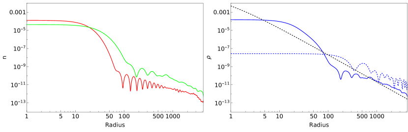
Figure 5: The same plots as in Fig. 4 with $\displaystyle m_{2}/m_{1}=1/2$ and starting from random initial conditions through Eqs. (37) and (38). The initial conditions do not seem to greatly impact the final result of the simulation: a virialized cored halo with an NFW tail. Here we can also clearly see the analogy to density granules in spherical symmetry: dips and peaks in the profile supported by pressure gradients.

The halo has the properties that we expect from ULDM: a centralized core with an NFW tail. Assuming that the typical velocities of the particles in the halo are the same, the lighter field has a larger De Broglie wavelength $\displaystyle\lambda=1/mv$. This can be seen especially in the core where the lighter field has a broader density profile. The overall mass density can thus transition between being dominated by the more massive field to being dominated by the lighter field, potentially leading to interesting observational signatures. Lastly, note that even though virialization happens faster in the case where we initialize with a Gaussian field profile (which makes intuitive sense as the phases of the fields are already correlated over large distances initially), the virialized final products of the simulations have similar properties across different initializations, in a way “erasing” the memory of the initial conditions.

An important question remains: are the cores of these halos the gravitational solitons found in Sec. II.2? To check this we take the final ratio of the density profiles of the two fields and use the algorithm of II.2 to solve the corresponding ground state solitons. The results are shown in Fig. 6

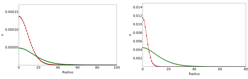
Figure 6: The number density profile of the heavy (red) and light (green) fields at the end of two of our simulations. In black dotted, we plot the corresponding two-field soliton that matches the central number density of the two fields. It is clear that the core of our halo is exactly one of the gravitational solitons found earlier in this work. Although here we only show the product of two simulations, we found that a nested two-field soliton can always be found at the center of a properly virialized halo, including for different mass ratios $\displaystyle m_{2}/m_{1}$. Left: $\displaystyle m_{2}/m_{1}=1/2$ Right: $\displaystyle m_{2}/m_{1}=1/5$.

It seems clear that the core of the halo can indeed be interpreted as a static solution of the two-field Schrödinger-Poisson system. Although these solitons are in principle static when isolated, we observe oscillation around the true static solution of $\displaystyle O(10\%)$, due to interactions with the halo. This is not altogether unexpected and can be explained as a wave-interference effect as was done in Li et al. (2021) and Lin et al. (2018). We also want to note that Refs. Huang et al. (2023); Luu et al. (2023) reported on certain situations (depending on the relative abundance of particles and the ratio of fundamental masses $\displaystyle m_{2}/m_{1}$) where the two-field soliton was not able to form due to tidal interactions between the different components during the formation of the halo. We wish to report that we did not observe this in our simulations. In particular, we always observed a two-field soliton at the center of the virialized halos that we generated. However, we acknowledge that this might in part be due to the limitations of imposing spherical symmetrie on our system.

Although we now have seen that a two-field soliton forms at the center of virialized halos, we still have no way to know what particular soliton should be present in what halo (e.g. what is the ratio of central densities of the two fields). To constrain multi-field models of ULDM, this is an important question to answer. Namely, we are interested in relating the properties of the halo to the solitonic core.

III.2.2 The relationship between the halo and the soliton

In studies of structure formation of (single-field) ULDM models, an interesting relation was discovered between core mass $\displaystyle M_{c}$ (mass contained in the region where the mass density remains $\displaystyle 50\%$ of the central density and the halo mass $\displaystyle M_{h}$. Previous work Schive et al. (2014b, a) found the following scaling

$$M_{c}\propto a^{-1/2}M_{h}^{1/3}$$ (40)

where $\displaystyle a$ is the scale factor of the Universe. This relation has been somewhat disputed in the literature Mocz et al. (2017); Bar et al. (2018); Levkov et al. (2018); Dmitriev et al. (2023), but most groups agree that some type of scaling is present, with (40) the most commonly cited one. Somehow, the wave nature of ULDM connects the properties of the central soliton to those of the enveloping halo. The question has to be asked whether a similar connection holds when considering multiple fields. In Bar et al. (2018) it was suggested that the scaling (40) can be explained through an empirical “thermodynamic” relation that is obeyed in the halo, namely

$$\frac{|E_{h}|}{M_{h}}=\frac{|E_{s}|}{M_{s}}$$ (41)

The energy per unit of mass has the same value in the halo and the central soliton. Using (41) together with some considerations from collapse models of overdensities, one can arrive at (40) rather straightforwardly. However, this is in large part due to the simple scaling of the single-field solitons, and a simple scaling like (40) is not expected to exist in our two-field system.

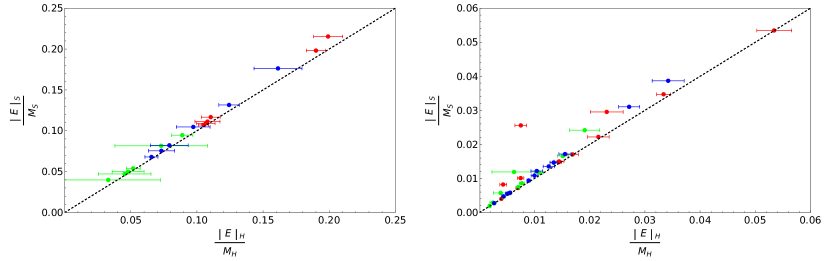
Figure 7: The energy per unit mass for the full halo obtained as the final product of our simulation (y-axis) versus the energy per unit mass for the soliton at the center (x-axis), for $\displaystyle m_{2}/m_{1}=1/2$. We plot the values for the heavy field (red), light field (green), and the full system (blue). In black dotted, we plot the line $\displaystyle y=x$. Although there remains large uncertainty, these results are highly suggestive. Left: starting from a Gaussian packet following Eqs. (35) and (36). Right: The same plot but for the halos obtained from random initialization following Eqs. (37) and (38).

However, we can ask if a relation like (41) still exists. In the multi-field case, there are more potential relations to be explored. In particular, we can consider the energy per unit mass in the system as a whole, but also at the level of each field individually. We checked this for the different virialized halos of our simulations by comparing the properties of the halo in the full numerical box with the ones of the soliton core. The properties of the core are taken by solving for the appropriate soliton solution, using the algorithm of Sec. II.2. We plot the results in Figs. 7 and 8, separating the different types of initializations we have considered.

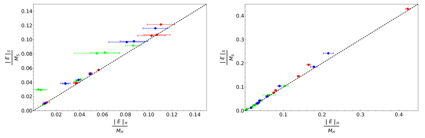
Figure 8: The same data as plotted in Fig. 7 starting from a Gaussian packet following Eqs. (35) and (36) for different mass ratios. We choose the Gaussian initialization because it tends to relax to a virialized halo faster, and thus speeds up computations. Left: $\displaystyle m_{2}/m_{1}=4/5$. Right: $\displaystyle m_{2}/m_{1}=1/5$. Qualitatively, the results agree with Fig. 7, namely that the energy per unit mass has the same value in the soliton, as it has in the halo.

Looking at Figs. 7 and 8, there seems to be fairly compelling evidence for the following three empirical relations:

$$\frac{|E_{h,tot}|}{M_{h,tot}}=\frac{|E_{s,tot}|}{M_{s,tot}};\quad\frac{|E_{h,\psi}|}{M_{h,\psi}}=\frac{|E_{s,\psi}|}{M_{s,\psi}};\quad\frac{|E_{h,\chi}|}{M_{h,\chi}}=\frac{|E_{s,\chi}|}{M_{s,\chi}}$$ (42)

Where the subscripts refer to the halo and soliton of the total system and the two fields individually. We want to place a caveat here, as we have to note that the radial simulations generally yielded halos whose masses were dominated by the central soliton. The relations in Eqs. (42) are then satisfied somewhat trivially. Checking whether these relations emerge in general is left for the future as it requires 3D simulations that go beyond the scope of this work.

Interestingly, if the relations in (42) hold generically, one is completely able to determine which solitonic core is present in which galaxy, based on the conserved quantities of the system, namely $\displaystyle E_{h}$, $\displaystyle M_{\psi}$ and $\displaystyle M_{\chi}$. There is exactly one soliton solution that can satisfy these properties and the system is neither over or under determined. Let’s outline an algorithm that can solve for a particular soliton solution, starting from $\displaystyle E_{h}$, $\displaystyle M_{\psi}$ and $\displaystyle M_{\chi}$.

1. Using the algorithm of Sec. II.2, we obtain a function of $\displaystyle|E_{s,fr,tot}|/M_{s,f,tot}$ for the soliton solutions with central densities $\displaystyle\Psi_{0}=1$ and $\displaystyle\Phi_{0}=f$. Through the scaling relations of Eqs. (28), (29) and (30), we then know what the scaling parameter $\displaystyle\lambda$ should be for each ratio of central densities in order to satisfy $\displaystyle|E_{h,tot}|/M_{h,tot}=|E_{s,f,tot}|/M_{s,f,tot}$.

2. Similarly, we can create functions $\displaystyle|E_{s,f,\psi}|/M_{s,f,\psi}$ and $\displaystyle|E_{s,f,\chi}|/M_{s,f,\chi}$. At each ratio of central density, we have to satisfy

   $$|E_{\psi}|=\lambda^{2}M_{\psi}\frac{|E_{s,f,\psi}|}{M_{s,f,\psi}}\quad\textrm{and}\quad|E_{\chi}|=\lambda^{2}M_{\chi}\frac{|E_{s,f,\chi}|}{M_{s,f,\chi}}$$ (43)

   Where at each ratio we have determined $\displaystyle\lambda$ in step 1.

3. Realising that $\displaystyle E_{\psi}+E_{\chi}=E_{h}$ and using Eq. (43) we can rewrite Eqs. (43) to obtain

   $$|E_{h}|=\lambda^{2}\left(M_{\psi}\frac{|E_{s,f,\psi}|}{M_{s,f,\psi}}+M_{\chi}\frac{|E_{s,f,\chi}|}{M_{s,f,\psi}}\right)$$ (44)

   This equation will only be satisfied for one particular ratio of central densities (and through step 1 $\displaystyle\lambda$). We will then have found the appropriate soliton solution.

This type of computation allows us to know what multi-field soliton should exist in a given halo when we know its conserved quantities. We will use this in the next section to discuss the cosmological implications of two-field ULDM.

IV Cosmological Implications

The major success of the ULDM paradigm lies in its ability to suppress structure on small scales, matching observations Rodrigues et al. (2017) . The presence of a solitonic core at the center of collapsed halos is a strong prediction and its properties can in principle be used to obtain observational constraints. In fact, in previous work one of us argued that the properties of the single-field solitons disfavor most ULDM models Deng et al. (2018). Central to the argument is the relation between the core central density $\displaystyle\rho_{c}$ and the core radius $\displaystyle R_{c}$ (the radius at which the soliton density drops by $\displaystyle 50\%$). The observational results, when fitting rotation curves with a cored density profile are given in Fig. 9.

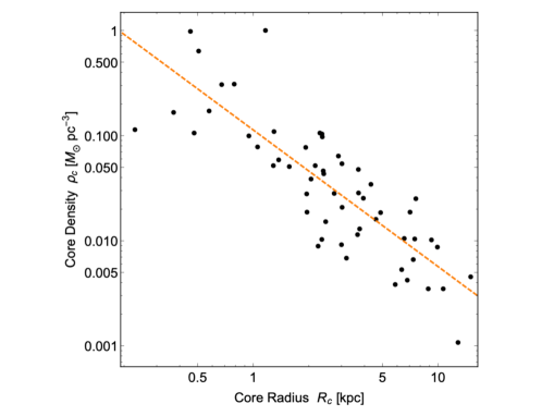
Figure 9: The best-fit parameters of the Core Density $\displaystyle\rho_{c}$ and Core Radius $\displaystyle R_{c}$ of 56 galaxies obtained from Rodrigues et al. (2014). The data suggests a scaling of $\displaystyle\rho_{c}\propto 1/R_{c}^{\beta}$ with $\displaystyle\beta\approx 1.3$. This puts a strain on all single-field ULDM models that generally predict a value of $\displaystyle\beta$ that is higher than this number. This apparent contradiction was first highlighted in Deng et al. (2018) (and this figure is reproduced from Ref. Deng et al. (2018)). As we’ll see, multi-field models alter this precise theoretical prediction.

Fig. 9 suggests a scaling of $\displaystyle\rho_{c}\propto 1/R_{c}^{\beta}$, with the best fit provided by $\displaystyle\beta\approx 1.3$. Now the problem arises: if the cores are really provided by gravitational solitons of the ULDM field, there are no single-field models that contain such a scaling. In particular, if the scalar has no self-interactions, the scaling is always $\displaystyle\rho_{c}\propto 1/R_{c}^{4}$. This can be easily seen through the transformation of Eq. (13). Interestingly, one finds more promise in the multi-field models under consideration here, as was first pointed out in Guo et al. (2021). As there are distinct soliton solutions at each ratio of the central density (not related through a simple scaling relation), the solitons interpolate between the two asymptotes where one of the fields dominates the mass, and we are again in the regime of $\displaystyle\rho_{c}\propto 1/R_{c}^{4}$. In this way a whole new region of parameter space becomes available. We show this schematically in Fig. 10.

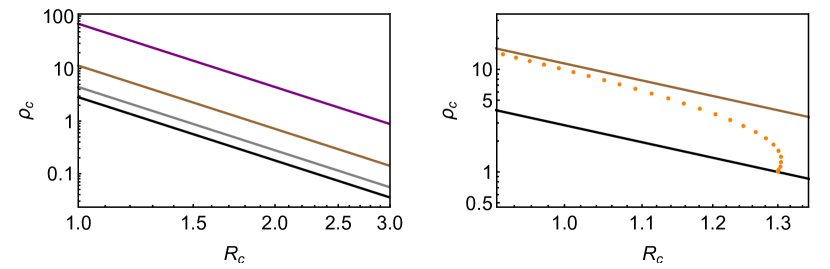
Figure 10: Left: The various scalings of $\displaystyle\rho_{c}$ versus $\displaystyle R_{c}$ for single-field gravitational solitons in terms of dimensionless variables. The single-field solitons all follow a scaling of $\displaystyle\rho_{c}\propto 1/R_{c}^{4}$. Here we plot the scalings corresponding to $\displaystyle m_{2}/m_{1}=1$ (black, the line corresponding to the heavy field), $\displaystyle m_{2}/m_{1}=4/5$ (gray), $\displaystyle m_{2}/m_{1}=1/2$ (brown) and $\displaystyle m_{2}/m_{1}=1/5$ (purple). Right: The full two-field gravitational soliton solutions with $\displaystyle m_{2}/m_{1}=0.5$ (orange scatter), where the ratio of central field values $\displaystyle\Phi_{0}/\Psi_{0}$ is increased from $\displaystyle 0$ to $\displaystyle\infty$. The full solution interpolates between the two asymptotes thus opening up the entire region of parameter space enclosed by these lines.

We now want to see whether the two-field scenario can actually solve the issue, considering the previous sections of this work. In particular, do we expect the solitons that form, to actually have the correct scaling? We want to note that in a similar way as schematically outlined above, multi-component ULDM can “escape” the constraints that exist for single-field models. In particular in Bar et al. (2018) a tension is highlighted, coming from rotation curve data. By opening up the parameter space of possible solitons that are present in the core, this apparent problem can also be alleviated.

To make comparisons with Cosmology we need to put back dimensions into our story. In order to do this we consider $\displaystyle m_{1}=5\cdot$\displaystyle 10\text{\times}{10}^{-22}\text{\,}\mathrm{eV}$$. Different mass ratios might be considered (and even match the data of Fig. 9 better), but won’t change the overall conclusions. As first noted in Guo et al. (2021), to accommodate all the galaxies in Fig. 9, we need at least $\displaystyle m_{2}/m_{1}\approx 10^{-3}$. Since it is numerically intense to generate data about the core solitons for these values of the mass ratio, we limit ourselves to the benchmark case of $\displaystyle m_{2}/m_{1}=1/2$. The overall, qualitative conclusions are valid for any value of the mass ratio.

Using the relations of Eq. (42) and the algorithm discussed at the end of Sec. III.2.2 we are able to generate a mock galaxy data set containing the information about the soliton expected to be present at the center of the halo. In order to do this we need to input the conserved quantities: the total energy $\displaystyle|E_{h}|$ and the masses of the two fields $\displaystyle M_{\psi}$ and $\displaystyle M_{\chi}$. We will assume that the energy of the halo is that of a non-moving overdensity of particles (so no kinetic energy), with a constant overdensity profile given by $\displaystyle\rho=10^{-5}\rho_{0}$ where $\displaystyle\rho_{0}=$\displaystyle 1.8\text{\times}{10}^{-9}\text{\,}\mathrm{eV}$^{4}$ matches the intergalactic (IGM) density of about 1 proton per cubic meter. The energy of such a cloud is then given by $\displaystyle E_{h}=-\frac{3}{5}\frac{GM^{5/3}\rho^{1/3}}{(3/4\pi)^{1/3}}$, with $\displaystyle M=M_{\psi}+M_{\chi}$ the total mass. To generate our set we then only need to make an assumption for the total mass in the galaxy $\displaystyle M$ and the relative abundance of the two species of particles $\displaystyle F=M_{\psi}/M_{\chi}$. To generate a mock sample of galaxies, we choose $\displaystyle M=10^{k}M_{MW}$, where k is taken from a uniform distribution with boundaries between $\displaystyle[-1,1]$. We use $\displaystyle M_{MW}=10^{12}M_{\odot}$, the Milky Way mass. Finally, we need to choose $\displaystyle F$. The most natural thing might be to assume that the relative abundance does not change with the galactic mass. However, it might also be interesting to investigate the possibility of $\displaystyle F$ depending on $\displaystyle M$. In particular, we will look at $\displaystyle F\propto M$ and $\displaystyle F\propto 1/M$, as well as $\displaystyle F=\mathrm{Const}$. To investigate an extremely exotic scenario we also looked at $\displaystyle F\propto M^{3}$. The proportionality factor is an $\displaystyle O(1)$ number in all cases. We plot the expected solitons for the four scenarios in Fig. 11. In each case, we choose the value of $\displaystyle F$ from a Gaussian distribution centered around its expected average value $\displaystyle\mu_{F}$ ($\displaystyle\mu_{F}=1/4$, $\displaystyle\mu_{F}\propto M$, $\displaystyle\mu_{F}\propto 1/M$, $\displaystyle\mu_{F}\propto M^{3}$, respectively) with a variance of $\displaystyle\sigma_{F}=0.25\mu_{F}$.

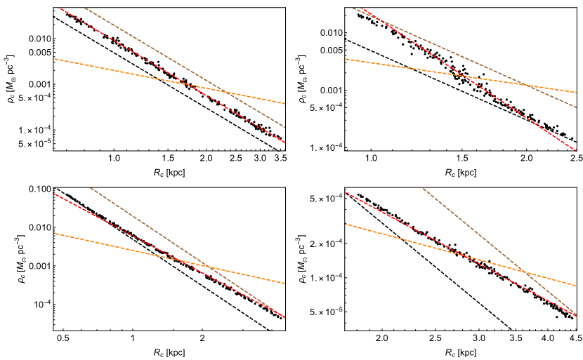
Figure 11: The properties of the solitons of our mock galaxy set as generated through the method highlighted in the text (black scatter). The properties of the single-field solitons of the heavy and light species are also shown (black and brown dotted). In each plot, we chose a different dependence for the ratio of total mass of each species $\displaystyle F$, with $\displaystyle F=1/4$ (top left), $\displaystyle F\propto M$ (bottom left), $\displaystyle F\propto 1/M$ (top right) and $\displaystyle F\propto M^{3}$ (bottom right). The emperical scaling of $\displaystyle\rho_{c}\propto 1/R_{c}^{1.3}$ is shown as the orange dotted line. As expected, the species that dominates the mass of the galaxy also dominates the soliton properties. We can thus find solitons living in the region of parameter space between the two extremal asymptotes. The scaling of $\displaystyle\rho_{c}$ versus $\displaystyle R_{c}$ can then differ from the single-field story. The red dotted line gives the approximate new scaling that emerges and in particular, we have $\displaystyle\rho_{c}\propto 1/R_{s}^{4}$ (top left), $\displaystyle\rho_{c}\propto 1/R_{s}^{3.2}$ (bottom left), $\displaystyle\rho_{c}\propto 1/R_{s}^{6}$ (top right) and $\displaystyle\rho_{c}\propto 1/R_{s}^{2.6}$ (bottom right). For the case that $\displaystyle F$ is positively correlated with the mass of the galaxy $\displaystyle M$, we see that the tension with Fig. 9 can be alleviated.

Inspecting Fig. 11 we see that non-trivial scalings only emerge when the ratio of masses in the galaxies is dependent on the total galaxy mass. This makes intuitive sense: if the ratio of masses is the same across every halo, one would expect that the ratio of core densities of the two fields is also the same. This is what happens in our mock data set. In this case, we are back in the scaling regime through the transformations of Eqs. (13), (14) and (15) and the soliton central density scales with $\displaystyle\rho_{c}\propto 1/R_{c}^{4}$. To reconcile the two-field model with Fig. 9 we need a non-trivial function for the mass ratio $\displaystyle F$. Allowing the halo to be dominated by different species in different limits of its total mass, causes the soliton solution to interpolate between the two asymptotic single-field solutions. This is the source of the non-trivial scaling. In particular, looking at Fig. 11, there needs to be a positive relation between the total mass $\displaystyle M$ of the halo and the ratio $\displaystyle F$. In other words, when the mass of the galaxy is large, the halo should be dominated by the heavier particles. The opposite scenario, where more massive galaxies are dominated by lighter particles, makes the situation worse. Of course, we could have chosen different functions for the ratio $\displaystyle F$, which would change the exact scaling of the galaxies in the interpolating region. It is an interesting question how the scaling depends exactly on this function. Investigating this and whether scenarios, where the relative abundance of particle species varies across different galaxies, can be accommodated in viable cosmological models goes beyond the scope of this work, although we plan to address it in future studies. It is clear, however, that multi-field models do not trivially solve the scaling issue highlighted in Deng et al. (2018). In appendix B we highlight another tension with experiment that seems generic for ULDM models and can not be alleviated by adding more fields to the picture. We will now summarize and conclude this work.

V Conclusions and Outlook

In this work we have examined two-field light scalar dark matter, focusing on their properties near the center of galaxies. While single scalar field models generally do not help to improve the fit to data Deng et al. (2018), the multi-field case has a larger phase space of solutions. The ratio of the fundamental particle’s masses provides a new parameter in the problem. The ratio of central densities provides a larger space of ground-state soliton solutions.

In this work, we have developed a new way to solve eigenstates of multi-component Ultra Light Dark Matter systems. Although we only used the method to find ground state solutions of fields with no (self)interactions, it is readily generalizable to include excited states and nonlinearities (other than gravity).

We have established some trends relating the core solutions to the halo properties to cut down the space of possibilities. we have found that if the relative abundances of the two species are comparable for different galaxies, then multi-field models do not provide an improved fit to the data. In fact this problem is worsened if the lighter species is more abundant in the heavier galaxies. However, if the lighter species is systematically less abundant in heavier galaxies, then there is improvement in the core density-radius relation.

There is some evidence in the literature that during the formation process of a halo, the lighter species can cause tidal stripping of the heavier species Huang et al. (2023); Luu et al. (2023). However, how this affects the final scaling relation of relative abundances deserves investigation.

Future work can involve 3-dimensional simulations, rather than the spherically symmetric simulations preformed here. Furthermore, more refined simulations would be useful to definitely establish the core-halo relations that we have seen here in this multi-field setup. Another possible option is to go beyond two-fields to $\displaystyle N$-fields. While we think the two-field case is indicative of the trend for larger $\displaystyle N$, relatively to the single species case, it is worth exploring in more detail. Also, large $\displaystyle N$ has a phenomenological motivation: ULDM single models lead to significant density fluctuations that can cause heating and redistribution of stars in a way that is incompatible with data Dalal and Kravtsov (2022). However, for large $\displaystyle N$ these density fluctuations are reduced as $\displaystyle\sim 1/\sqrt{N}$ due to a random walk; hence the heating effects should become negligible. Then the core-halo and core-radius relations become critical, as we have explored here.

VI Acknowledgements

We thank Rodrigo Vicente and Demao Kong for various useful discussions. We are also thankful to Davi Rodrigues for providing the empirical data we present in Appendix B and which is first presented in Refs. Rodrigues et al. (2014, 2017). We aslo thank him for useful remarks on the draft of this paper. M. P. H. is supported in part by National Science Foundation grant PHY-2310572. F. D. acknowledges the support from the Departament de Recerca i Universitats from Generalitat de Catalunya to the Grup de Recerca 00649 (Codi: 2021 SGR 00649) and funding from the ESF under the program Ayudas predoctorales of the Ministerio de Ciencia e Innovación PRE2020-094420.

Appendix A Ground State Gravitational Solitons

It is important to check whether the method highlighted in section II.2 actually yields ground state solutions of the two-field SP system. In order to check this explicitly we ran simulations where the initial conditions were set to be exactly one of the zero-node solutions we found using the algorithm of Sec. II.2. A proper ground state of the system should have a constant density profile for many periods of oscillations in complex fieldspace. We found that this is the case for all our zero-node solutions. To check these properties it is useful to define the following quantities

$$\frac{|\delta n_{\psi}(0,t)|}{n_{\psi}(0,0)}=\frac{|1-|\psi(0,t)|^{2}|}{|\psi(0,t)|^{2}}\quad\textrm{and}\quad\frac{|\delta n_{\chi}(0,t)|}{n_{\chi}(0,0)}=\frac{|1-|\chi(0,t)|^{2}|}{|\chi(0,t)|^{2}}$$ (45)

$$\frac{|1-N_{50,\psi}(t)|}{N_{50,\psi}(0)}\quad\textrm{and}\quad\frac{|1-N_{50,\chi}(t)|}{N_{50,\chi}(0)}$$ (46)

Where we define $\displaystyle N_{50}$ as the total amount of particles in each species, within the radius that initially contains $\displaystyle 50\%$ of the total amount of particles of that species. In Figs. 12 and  13 we show this for two benchmark cases in which the two fields have comparable mass content and central density (in particular, the magenta ($\displaystyle m_{2}/m_{1}=1/2$) and cyan ($\displaystyle m_{2}/m_{1}=1/5$) profiles of Fig. 1).

As is expected of ground state solitons the quantities defined in Eqs. (45) and (46) are conserved for these solutions up to at most one part in one hundred (which is also somewhat dependent on the resolution of the simulation). This indicates that both the central densities and overall density profile of the two species stay constant. Finally, we observe that the real and imaginary parts of the two fields oscillate out of phase (with a phase-shift of $\displaystyle\pi/2$) as is to be expected of an eigenstate of the system. Interestingly the periods of oscillation need not be the same and can differ widely. These results for the benchmark cases, where both species have comparable total mass give us confidence in concluding that our algorithm is sufficient to find the ground state solitons of the two-field SP system.

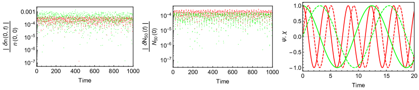
Figure 12: Some of the dynamical properties of the benchmark soliton for $\displaystyle m_{2}/m_{1}=1/2$ (the magenta profile in Fig. 1). Left: The relative variation of the central density as defined in (45) for the heavy field $\displaystyle\psi$ (red) and the light field $\displaystyle\chi$ (green). Middle: The relative variation of the density profile as defined through (46) for the heavy field $\displaystyle\psi$ (red) and the light field $\displaystyle\chi$ (green). Right: The real (full) and imaginary (dashed) parts of the heavy field $\displaystyle\psi$ (red) and the light field $\displaystyle\chi$ (green) at the origin. As expected the real and imaginary parts oscillate out-of-phase with a phase shift of $\displaystyle\pi/2$.

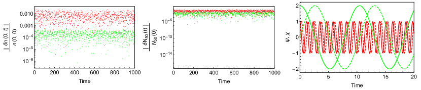
Figure 13: Some of the dynamical properties of the benchmark soliton for $\displaystyle m_{2}/m_{1}=1/5$ (the cyan profile in bottom panel of Fig. 1). Left: The relative variation of the central density as defined in (45) for the heavy field $\displaystyle\psi$ (red) and the light field $\displaystyle\chi$ (green). Middle: The relative variation of the density profile as defined through (46) for the heavy field $\displaystyle\psi$ (red) and the light field $\displaystyle\chi$ (green). Right: The real (full) and imaginary (dashed) parts of the heavy field $\displaystyle\psi$ (red) and the light field $\displaystyle\chi$ (green) at the origin. As expected the real and imaginary parts oscillate out-of-phase with a phase shift of $\displaystyle\pi/2$.

Appendix B Relation between Soliton Properties and Halo Mass

There is another hidden prediction in the generated datasets of Sec. IV. In particular, it relates the total mass of each galaxy to the central core properties. To zeroth-order it is simple to see how these quantities are correlated in the mock galaxy sets we generated. In particular, with the assumptions taken, the energy per unit mass of the halo is positively correlated to the halo mass: $\displaystyle E_{h}/M_{h}\propto M_{h}^{2/3}$. If we were dealing with a single-field system and the energy per unit mass in the halo were the same as in the soliton (as we’re assuming here), we would immediately conclude that the mass of the soliton scales as $\displaystyle M_{s}\propto\lambda M_{0}=M_{h}^{1/3}M_{0}$, as suggested in Eq. (40). At zeroth-order there then should be a positive correlation between the soliton mass and the halo mass. In the single-field limit, this translates into a positive correlation between core density and halo mass, and a negative correlation between core radius and halo mass. We show in Fig. 15 what the behavior is for the galaxies generated in Sec. IV. The same conclusions hold in our two-field model although there is not as simple a scaling as in Eq. (40). We can compare this prediction with empirical data from Rodrigues et al. (2014) and Rodrigues et al. (2017). Combining the two sources we obtain estimates of core properties and halo masses for 56 galaxies. The estimates are obtained by fitting rotation curves with different DM density profiles. In particular, the virial mass plotted here $\displaystyle M_{vir}$ corresponds to the mass of the best-fit NFW profile integrated up to $\displaystyle r_{200}$, defined through

$$M_{NFW}(r_{200})=200\frac{4\pi}{3}r_{200}^{3}\rho_{\mathrm{crit}}$$ (47)

Where $\displaystyle\rho_{\mathrm{crit}}$ is the critical cosmological density. We want to note that the exact definition of the virial mass impacts the implied virial mass. In general, it is not easy to find a consistent definition of the mass of a galaxy, that is exempt from systematics. In particular, using different fits for the density profiles of galaxies will lead to a different implied virial mass. For example, in other works the Burkert profile was used to fit rotation curves and derive the mass of each galaxy Li et al. (2020); Rodrigues et al. (2023), changing the results somewhat. The results are plotted in Figs. 14.

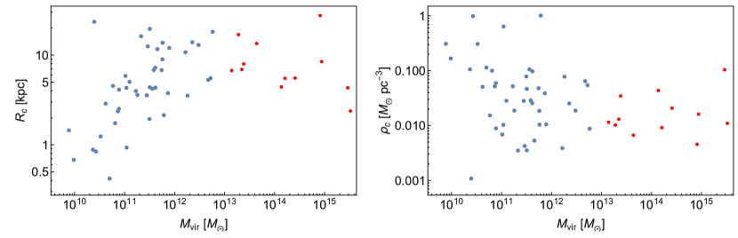
Figure 14: The core density and radius versus the total virial mass for the galaxies of Fig. 9. The data approximately follows a power law curve $\displaystyle\propto x^{\beta}$, especially if we exclude galaxies that we consider to have unphysical masses of $\displaystyle M_{vir}>10^{13}M_{\odot}$ (which are plotted in red here). Even with this exclusion, however, the correlation is not very strong. Nonetheless, a positive correlation between the core radius and virial mass, and a negative correlation between the core density and virial mass can be seen. This contradicts the scaling of Eq. (40) as well as the mock galaxies of Sec. IV.

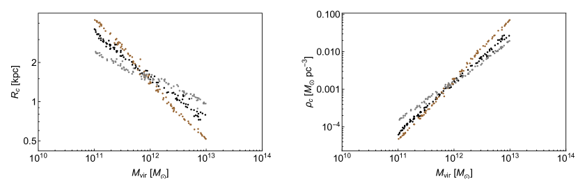
Figure 15: The core density and radius versus the total virial mass for the galaxies of Fig. 11. The black dotted line is the best-fit correlation extracted from empirical data of Fig. 14. We plot the galaxies generated with $\displaystyle F=1/4$ (black), $\displaystyle F\propto M$ (brown) and $\displaystyle F\propto 1/M$ (gray). None of the mock sets seems to obey the weak correlation between total mass $\displaystyle M_{vir}$ and core properties seen in the empirical data above of Fig. 14.

Although the correlations are weak, the data seems to suggest the opposite with respect to the Ultra Light Dark Matter models that are the subject of this work. In particular, a positive correlation between the core radius and virial mass, and a negative correlation between the core density and virial mass. This puts strain on both the single-field models suggesting the scaling of Eq. (40), as well as the multi-field models, the subject of this work. There is however large uncertainty in these conclusions, as the correlation in the experimental data is weak, and furthermore, the definition of the virial mass is not exempt from systematics. A more comprehensive and complete analysis of the relation between the core properties and halo mass of various galaxies is an interesting avenue for future research.

References

- Arvanitaki et al. (2010) Asimina Arvanitaki, Savas Dimopoulos, Sergei Dubovsky, Nemanja Kaloper, and John March-Russell, “String axiverse,” Physical Review D 81 (2010), 10.1103/physrevd.81.123530.
- Hu et al. (2000) Wayne Hu, Rennan Barkana, and Andrei Gruzinov, “Cold and fuzzy dark matter,” Phys. Rev. Lett. 85, 1158–1161 (2000), arXiv:astro-ph/0003365 .
- Dalal and Kravtsov (2022) Neal Dalal and Andrey Kravtsov, “Not so fuzzy: excluding fdm with sizes and stellar kinematics of ultra-faint dwarf galaxies,” (2022), arXiv:2203.05750 [astro-ph.CO] .
- Irš ič et al. (2017) Vid Irš ič, Matteo Viel, Martin G. Haehnelt, James S. Bolton, and George D. Becker, “First constraints on fuzzy dark matter from lyman-alpha forest data and hydrodynamical simulations,” Physical Review Letters 119 (2017), 10.1103/physrevlett.119.031302.
- Armengaud et al. (2017) Eric Armengaud, Nathalie Palanque-Delabrouille, Christophe Yè che, David J. E. Marsh, and Julien Baur, “Constraining the mass of light bosonic dark matter using SDSS lyman-alpha forest,” Monthly Notices of the Royal Astronomical Society 471, 4606–4614 (2017).
- Chan et al. (2022) Hei Yin Jowett Chan, Elisa G M Ferreira, Simon May, Kohei Hayashi, and Masashi Chiba, “The diversity of core–halo structure in the fuzzy dark matter model,” Monthly Notices of the Royal Astronomical Society 511, 943–952 (2022).
- Powell et al. (2023) Devon M Powell, Simona Vegetti, J P McKean, Simon D M White, Elisa G M Ferreira, Simon May, and Cristiana Spingola, “A lensed radio jet at milli-arcsecond resolution – II. constraints on fuzzy dark matter from an extended gravitational arc,” Monthly Notices of the Royal Astronomical Society: Letters 524, L84–L88 (2023).
- Hertzberg and Loeb (2023) Mark P. Hertzberg and Abraham Loeb, “Quantum tunneling of ultralight dark matter out of satellite galaxies,” JCAP 02, 059 (2023), arXiv:2212.07386 [astro-ph.CO] .
- Huang et al. (2023) Hsinhao Huang, Hsi-Yu Schive, and Tzihong Chiueh, “Cosmological simulations of two-component wave dark matter,” Monthly Notices of the Royal Astronomical Society 522, 515–534 (2023).
- Luu et al. (2023) Hoang Nhan Luu, Philip Mocz, Mark Vogelsberger, Simon May, Josh Borrow, S. H. Henry Tye, and Tom Broadhurst, “Nested solitons in two-field fuzzy dark matter,” (2023), arXiv:2309.05694 [astro-ph.CO] .
- Gosenca et al. (2023) Mateja Gosenca, Andrew Eberhardt, Yourong Wang, Benedikt Eggemeier, Emily Kendall, J. Luna Zagorac, and Richard Easther, “Multifield ultralight dark matter,” Physical Review D 107 (2023), 10.1103/physrevd.107.083014.
- Glennon et al. (2023) Noah Glennon, Nathan Musoke, and Chanda Prescod-Weinstein, “Simulations of multifield ultralight axionlike dark matter,” Physical Review D 107 (2023), 10.1103/physrevd.107.063520.
- Jain et al. (2023) Mudit Jain, Mustafa A. Amin, Jonathan Thomas, and Wisha Wanichwecharungruang, “Kinetic relaxation and bose-star formation in multicomponent dark matter- i,” (2023), arXiv:2304.01985 [astro-ph.CO] .
- Eby et al. (2020) Joshua Eby, Madelyn Leembruggen, Lauren Street, Peter Suranyi, and L.C.R. Wijewardhana, “Galactic condensates composed of multiple axion species,” Journal of Cosmology and Astroparticle Physics 2020, 020–020 (2020).
- Amin et al. (2022) Mustafa A. Amin, Mudit Jain, Rohith Karur, and Philip Mocz, “Small-scale structure in vector dark matter,” Journal of Cosmology and Astroparticle Physics 2022, 014 (2022).
- Rodrigues et al. (2017) Davi C. Rodrigues, Antonino del Popolo, Valerio Marra, and Paulo L. C. de Oliveira, “Evidence against cuspy dark matter haloes in large galaxies,” Monthly Notices of the Royal Astronomical Society 470, 2410–2426 (2017).
- Deng et al. (2018) Heling Deng, Mark P. Hertzberg, Mohammad Hossein Namjoo, and Ali Masoumi, “Can light dark matter solve the core-cusp problem?” Physical Review D 98 (2018), 10.1103/physrevd.98.023513.
- Guo et al. (2021) Huai-Ke Guo, Kuver Sinha, Chen Sun, Joshua Swaim, and Daniel Vagie, “Two-scalar bose-einstein condensates: from stars to galaxies,” Journal of Cosmology and Astroparticle Physics 2021, 028 (2021).
- Chavanis (2011) Pierre-Henri Chavanis, “Mass-radius relation of Newtonian self-gravitating Bose-Einstein condensates with short-range interactions: I. Analytical results,” Phys. Rev. D 84, 043531 (2011), arXiv:1103.2050 [astro-ph.CO] .
- Chavanis and Delfini (2011) P. H. Chavanis and L. Delfini, “Mass-radius relation of Newtonian self-gravitating Bose-Einstein condensates with short-range interactions: II. Numerical results,” Phys. Rev. D 84, 043532 (2011), arXiv:1103.2054 [astro-ph.CO] .
- Schiappacasse and Hertzberg (2018) Enrico D. Schiappacasse and Mark P. Hertzberg, “Analysis of Dark Matter Axion Clumps with Spherical Symmetry,” JCAP 01, 037 (2018), [Erratum: JCAP 03, E01 (2018)], arXiv:1710.04729 [hep-ph] .
- Visinelli et al. (2018) Luca Visinelli, Sebastian Baum, Javier Redondo, Katherine Freese, and Frank Wilczek, “Dilute and dense axion stars,” Phys. Lett. B 777, 64–72 (2018), arXiv:1710.08910 [astro-ph.CO] .
- Schive et al. (2014a) Hsi-Yu Schive, Tzihong Chiueh, and Tom Broadhurst, “Cosmic structure as the quantum interference of a coherent dark wave,” Nature Physics 10, 496–499 (2014a).
- Schive et al. (2014b) Hsi-Yu Schive, Ming-Hsuan Liao, Tak-Pong Woo, Shing-Kwong Wong, Tzihong Chiueh, Tom Broadhurst, and W-Y. Pauchy Hwang, “Understanding the core-halo relation of quantum wave dark matter from 3d simulations,” Physical Review Letters 113 (2014b), 10.1103/physrevlett.113.261302.
- Guzmá n and Ureña-López (2004) F. Siddhartha Guzmá n and L. Arturo Ureña-López, “Evolution of the schrödinger-newton system for a self-gravitating scalar field,” Physical Review D 69 (2004), 10.1103/physrevd.69.124033.
- Hui et al. (2017) Lam Hui, Jeremiah P. Ostriker, Scott Tremaine, and Edward Witten, “Ultralight scalars as cosmological dark matter,” Physical Review D 95 (2017), 10.1103/physrevd.95.043541.
- Li et al. (2021) Xinyu Li, Lam Hui, and Tomer D. Yavetz, “Oscillations and random walk of the soliton core in a fuzzy dark matter halo,” Physical Review D 103 (2021), 10.1103/physrevd.103.023508.
- Lin et al. (2018) Shan-Chang Lin, Hsi-Yu Schive, Shing-Kwong Wong, and Tzihong Chiueh, “Self-consistent construction of virialized wave dark matter halos,” Physical Review D 97 (2018), 10.1103/physrevd.97.103523.
- Mocz et al. (2017) Philip Mocz, Mark Vogelsberger, Victor H. Robles, Jesú s Zavala, Michael Boylan-Kolchin, Anastasia Fialkov, and Lars Hernquist, “Galaxy formation with BECDM – i. turbulence and relaxation of idealized haloes,” Monthly Notices of the Royal Astronomical Society 471, 4559–4570 (2017).
- Bar et al. (2018) Nitsan Bar, Diego Blas, Kfir Blum, and Sergey Sibiryakov, “Galactic rotation curves versus ultralight dark matter: Implications of the soliton-host halo relation,” Physical Review D 98 (2018), 10.1103/physrevd.98.083027.
- Levkov et al. (2018) D. G. Levkov, A. G. Panin, and I. I. Tkachev, “Gravitational bose-einstein condensation in the kinetic regime,” Physical Review Letters 121 (2018), 10.1103/physrevlett.121.151301.
- Dmitriev et al. (2023) A. S. Dmitriev, D. G. Levkov, A. G. Panin, and I. I. Tkachev, “Self-similar growth of bose stars,” (2023), arXiv:2305.01005 [astro-ph.CO] .
- Rodrigues et al. (2014) Davi C. Rodrigues, Paulo L. de Oliveira, Jú lio C. Fabris, and Gianfranco Gentile, “Modified gravity models and the central cusp of dark matter haloes in galaxies,” Monthly Notices of the Royal Astronomical Society 445, 3823–3838 (2014).
- Li et al. (2020) Pengfei Li, Federico Lelli, Stacy McGaugh, and James Schombert, “A comprehensive catalog of dark matter halo models for SPARC galaxies,” The Astrophysical Journal Supplement Series 247, 31 (2020).
- Rodrigues et al. (2023) Davi C. Rodrigues, Alejandro Hernandez-Arboleda, and Aneta Wojnar, “Normalized additional velocity distribution: Testing the radial profile of dark matter halos and MOND,” Physics of the Dark Universe 41, 101230 (2023).