Kerner equation for motion in a non-Abelian gauge field

Abstract

The equations of motion of an isospin-carrying particle in a Yang-Mills and gravitational field were first proposed in 1968 by Kerner, who considered geodesics in a Kaluza-Klein-type framework. Two years later the flat space Kerner equations were completed by considering also the motion of the isospin by Wong, who used a field-theoretical approach. Their groundbreaking work was then followed by a long series of rediscoveries whose history is reviewed. The concept of isospin charge and the physical meaning of its motion are discussed. Conserved quantities are studied for Wu-Yang monopoles and for diatomic molecules by using van Holten’s algorithm.

I Introduction: a short history of the isospin

Certain ideas are put forward, then forgotten, and then reproposed again by various authors who ignore previous, and indeed each other’s work. A typical example is that of an isospin-carrying particle moving in a Yang-Mills field, first studied by Kerner Kerner68  :

Figure 1: :

Kerner’s paper in which the equation for a particle in a Non-Abelian gauge field was proposed.

Two years after Kerner’s pioneering paper Wong Wong70 , who ignored all about Kerner’ work and used a different, field-theoretical framework, completed the Kerner equations (II.17) below which describe motion in ordinary space-time, with one for the dynamics of the isospin, eqn. (II.18).

Their work was subsequently continued by many other researchers Trautman70 ; Cho75 ; Balachandran76 ; Balachandran77 ; Sternberg77 ; Sternberg78 ; Weinstein78 ; Sternberg80 ; DuvalCRAS ; DuvalAix79 ; DH82 ; Montgomery ; FeherAPH . Jackiw and Manton JackiwManton , searching for a physical interpretation of some quantities found in the study of the symmetries of gauge fields (re)covered the Kerner equation (II.17) from a partial variational principle, while assuming the isospin-equation (II.18).

These studies were parallelled by physical applications which include motion in the field of a non-Abelian monopole GoddardOlive , which requires extension to Yang-Mills-Higgs systems Feher:1984ik ; Feher:1984xc ; Feher86 ; Feher:1988th .

Yet another application is to the non-Abelian Aharonov experiment proposed by Wu and Yang WuYang75 ; WY76 , elaborated in HPNABA which will be further studied in EZH-NABA . The effect is related to topological defects Alford90 ; Preskill90 ; Brandenberger93 and more recently, it to artificial gauge fields which can be produced in laboratory Osterloh ; Dalibard ; Goldman ; Jacob ; YChen ; YYang ; YBiao ; Cserti .

As physical illustration, we derive conserved quantities for Wu-Yang monopoles WuYang69 and for diatomic molecules MSW ; Jackiw86 .

This review celebrates the 80th birthday of Richard Kerner by recounting the fascinating story of isospin-carrying particles initiated by him when his given name was still “Ryszard”.

II Gauge theory and the Kaluza-Klein framework

II.1 Yang-Mills theory

The concept of isotopic spin (in short: isospin) was introduced by Heisenberg in 1932 Heisenberg32 , who argued that a proton and a neutron should be viewed as two different states of the same particle, related by an “internal” $\mathrm{SU}(2)$ rotation .

Let us recall that electrodynamics is an Abelian gauge theory: it is described by a real 1-form $A=A_{\mu}dx^{\mu}$ called the vector potential which is however determined only up to a gauge transformation,

$$A_{\mu}\to A_{\mu}-i{}g^{-1}{\partial}_{\mu}g\,,$$ (II.1)

where $g(x^{\mu})$ is an ${\rm U}(1)$-valued function on space-time.

Twenty years later, Yang and Mills (YM) generalized Maxwell’s theory to non-Abelian fields which take their values in the Lie algebra $\mathfrak{G}={\mathrm{su}}(2)$ and can thus be acted upon by $G=\mathrm{SU}(2)$-valued gauge transformations YangMills ; AbersLee . In detail, YM fields are described by the Yang-Mills potential represented either by a $3$-vector ${\bm{A}}=(A_{\mu}^{a}),\,a=1,2,3$ or alternatively, by antihermitian ${\mathrm{su}}(2)$ matrices, $A_{\mu}=A_{\mu}^{a}\,\hbox{$\textstyle\frac{1}{2i}$}\sigma_{a}$, where the sigmas are the Pauli matrices

$$\sigma_{1}={\tiny\left(\begin{array}[]{cc}0&1\\ 1&0\end{array}\right)}\,,\;\;\sigma_{2}={\tiny\left(\begin{array}[]{cc}0&-i\\ i&0\end{array}\right)}\,,\;\;\sigma_{3}={\tiny\left(\begin{array}[]{cc}1&0\\ 0&-1\end{array}\right)}\,.$$

which satisfy $[\sigma_{a},\sigma_{b}]=2i\epsilon_{abc}\sigma_{c}$. In what follows we shall use mainly the matrix-formalism. Space-time indices will be denoted by greek letters, typically $\mu,\nu,\dots$ etc. Latin characters $a,b\dots$ are used for the internal, isospin indices. The Lie bracket in ${\mathrm{su}}(2)$ is $\big{(}[A,B]\big{)}^{a}=\epsilon^{a}_{\;bc}A^{b}B^{c}$. The field strength of a Yang-Mills field is

$$F={\scriptstyle{\frac{1}{2}}}F_{\mu\nu}dx^{\mu}\wedge dx^{\nu}{\quad\text{\small where}\quad}F_{\mu\nu}={\partial}_{\mu}A_{\nu}-{\partial}_{\nu}A_{\mu}+\big{[}A_{\mu},A_{\mu}]\,.$$ (II.2)

The Lie algebra carries a metric given by the trace form, $g_{ab}A^{a}B^{b}=-2\mathrm{tr}(AB)$ we denote also by $A\cdot B$. For ${\mathrm{su}}(2),\,g_{ab}=\delta_{ab}$.

The fundamental property of Yang-Mills theory is its behavior under an $\mathrm{SU}(2)$-valued gauge transformation YangMills ,

$$A_{\mu}\to g^{-1}A_{\mu}\,g+g^{-1}\partial_{\mu}g\,,\qquad F_{\mu\nu}\to g^{-1}F_{\mu\nu}\,g\,,$$ (II.3)

where $g(x^{\mu})\in\mathrm{SU}(2)$. A particle is coupled to the electromagnetic field $A_{\mu}$ by minimal coupling, which amounts to replacing ordinary derivatives by gauge-covariant derivatives AbersLee ,

$${\partial}_{\mu}\to{\partial}_{\mu}-i\,A_{\mu}\,,$$ (II.4)

where the electric charge was scaled to one. In Kerner68 Kerner argued that in a YM gauge field, this prescription should be replaced by an expression which (i) describes the properties of proton/neutron type “particles with internal YM structure” (ii) couples such a particle to the non-Abelian gauge potential : the rule (II.4) should be by generalized to

$${\partial}_{\mu}\to{\partial}_{\mu}+{\,}A_{\,\mu}$$ (II.5)

acting on fields in the fundamental representation. The non-Abelian coupling constant is scaled to unity.

What is the dynamics of such an isospin-carrying particle (also called a particle with internal YM structure) ? Kerner answers the question by considering a non-Abelian generalization of Kaluza-Klein (KK) theory Kaluza ; OKlein .

II.2 Abelian Kaluza-Klein theory

Electromagnetism and gravitation have been unified into a geometrical framework (now called fiber bundle theory) by Kaluza Kaluza and by Klein OKlein about 100 years ago .

It is assumed that the world has four spatial dimensions but one of the them we denote by $x^{5}$ has curled up to form a circle so small as to be unobservable. The basic assumption is that the correct vacuum is $M^{4}\times{\mathds{S}}^{1}_{R}$, the product of four dimensional Minkowski space with coordinates $x^{\mu},\,\mu=0,1,2,3$, with an internal circle of radius $R$.

Then general relativity in five dimensions contains a local U(1) gauge symmetry arising from the isometry of the hidden fifth dimension. The extra components of the metric tensor constitute the gauge fields and could be identified with the electromagnetic vector potential.

The theory is invariant under general coordinate transformations that are independent of $x^{5}$. In addition to ordinary four dimensional coordinate transformations, we have a U(1) local gauge transformation

$$x^{5}\to x^{5}+\Lambda(x^{\mu})$$ (II.6)

under which the $g_{\mu 5}$ component transforms as a ${\rm U}(1)$ gauge field,

$$g_{\mu 5}(x)\to g_{\mu 5}(x)+{\partial}_{\mu}\Lambda.$$ (II.7)

We write the metric with indices $A=\mu,5$ as,

$$ds^{2}=g_{AB}dx^{A}dx^{B}{\quad\text{\small where}\quad}g_{AB}=\left(\begin{array}[]{cc}g_{\mu\nu}+A_{\mu}A_{\nu}&A_{\mu}\\[1.0pt] A_{\nu}&1\end{array}\right)\,,$$ (II.8)

i.e.,

$$ds^{2}=g_{\mu\nu}dx^{\mu}dx^{\nu}+(dx^{5}+A_{\mu}dx^{\mu})^{2}\,.$$ (II.9)

Expressing the 5-dimensional scalar curvature $R_{5}$ in 4-dimensional terms, $R_{5}=R_{4}+\hbox{$\textstyle\frac{1}{4}$}F_{\mu\nu}F^{\mu\nu}$ where $R_{4}$ is the $4$-dimensional curvature, the effective low-energy theory is described by the four-dimensional action

$$S=-\frac{1}{16\pi G}\int d^{4}x\,\sqrt{-{\rm det}\,(g_{\mu\nu})}{\;}\Big{(}R_{4}+\hbox{$\textstyle\frac{1}{4}$}F_{\mu\nu}F^{\mu\nu}\Big{)},$$ (II.10)

where $G={G_{K}}/{2\pi R}$ is Newton’s constant. The internal radius $R$ is determined by the electric charge. The motion is given by a five-dimensional geodesic,

$$\frac{d^{2}x^{A}}{d\tau^{2}}+\Gamma^{A}_{\ BC}\,\frac{dx^{B}}{d\tau\;}\frac{dx^{C}}{d\tau\;}=0\,.$$ (II.11)

The KK space-time possesses a Killing vector, namely

$$K^{A}\frac{\ \partial}{\partial x^{A}}=\frac{\ \partial}{\partial x^{5}}\,,$$ (II.12)

which implies that

$$q=K_{A}\frac{dx^{A}}{d\tau}=\frac{dx^{5}}{d\tau}+A_{\mu}\frac{dx^{\mu}}{d\tau}$$ (II.13)

is a constant of the motion identified with the conserved electric charge. The remaining equations of motion then take the form,

$$\frac{d^{2}x^{\mu}}{d\tau^{2}}+\Gamma^{\mu}_{\alpha\beta}\frac{dx^{\alpha}}{d\tau}\frac{dx^{\beta}}{d\tau}=q\,\big{(}g^{\mu\alpha}F_{\alpha\nu}\big{)}\frac{dx^{\nu}}{d\tau}\,,$$ (II.14)

where $\Gamma^{\mu}_{\alpha\beta}$ is the Levi-Civita connection constructed from the four dimensional metric $g_{\mu\nu}$. On the right we recognize the Lorentz force. of electromagnetism.

II.3 Non-Abelian generalization

Kerner, in his groundbreaking paper Kerner68 , proposed to derive the dynamics of an isospin-carrying particle in a Yang-Mills (YM) field by generalizing the Abelian KK framework to non-Abelian gauges. His framework was further generalized Cho75 and applied later to particle motion in a Yang-Mills field by projecting the geodesic motion to $4D$ space FeherAPH . His clue [eqn. #(12) of Kerner68 ] is to replace the internal circle U(1) in the 5th dimension by the non-Abelian gauge group, $\mathrm{SU}(2)$ and the gauge potential in (II.8) by its non-Abelian counterpart. The key new ingredient w.r. t. electromagnetism is the isospin, represented by an ${\mathrm{su}}(2)$ matrix,

$$Q=Q^{a}\,\frac{1}{2i}\sigma_{a}\in{\mathrm{su}}(2)\,,$$ (II.15)

which couples the particle to the YM field introduced in sec.II.1, $A^{a}_{\,\mu}$ and $F^{a}_{\;\alpha\beta}$, respectively. The covariant derivative is

$$D_{\mu}Q={\partial}_{\mu}Q+[A_{\mu},Q]\,.$$ (II.16)

The ${\mathrm{su}}(2)$-valued YM potential is implemented on the isospin $Q\in{\mathrm{su}}(2)$ by commutation.

In a judicious coordinate system chosen by Kerner Kerner68 , the equations of motion for a test particle in the combined gravitational and gauge fields simplify to his eqn. # (34),

$$\;\;\displaystyle{\frac{d^{2}x^{\mu}}{ds^{2}}+\Gamma^{\mu}_{\alpha\beta}\frac{dx^{\alpha}}{ds}\,\frac{dx^{\beta}}{ds}=\big{(}g_{ab}Q^{b}\big{)}\,\big{(}g^{\mu\alpha}F^{a}_{\;\alpha\beta}\big{)}\frac{dx^{\beta}}{ds}\,.}\;\;$$ (II.17)

Generalizing the gauge group from U(1) of electromagnetism to the Yang-Mills gauge group $\mathrm{SU}(2)$ has a price to pay, though: unlike the electric charge in the electromagnetic theory which is a conserved scalar, the isospin has indeed its own dynamics : it is not a constant but a vector which (as Kerner puts it) “rotates, depending on the external field”.

The equations for the motion of the isospin,

$$\dot{Q}=[{Q},A_{\nu}\dot{x}^{\nu}]\,,$$ (II.18)

[where the “dot” is $d/{ds}$] were spelt out two years later by Wong Wong70 . In a geometric language, the isospin is parallel transported along the space-time trajectory, $x(t)=(x^{\mu})$. Written in terms of the covariant derivative (II.16),

$$\;\;\displaystyle{D_{s}{Q}\;\equiv\;\dot{Q}+\left[A_{\nu}\dot{x}^{\nu},{Q}\right]=0\,}\;\;$$ (II.19)

this equations says that the isospin is covariantly (but not ordinarily) conserved. Eqn. (II.18) is consistent with Kerner’s words, though, and also with what Yang and Mills say in their YangMills , where they mention “isospin rotation”.

One can wonder why did Kerner not spelt out the equations of motion for the isospin explicitly. A real answer can be given only by him, however one can try to guess what he might have had in his mind. One good reason might well have been that considering the isospin as a non-constant non-Abelian analog of the constant electric charge could have appeared too radical and even shocking, and be therefore discarded .

There might exist also other, subtle reasons related to the gauge invariance and the consequent problems of physical interpretation Arodz82 ; HRawnsley ; HRcolor . Another one could come from the experimental side.

Wong’s approach Wong70 is radically different from that of Kerner : instead of generalizing the classical dynamics of a charged particle moving in a curved space, he “dequantizes” the Dirac equation. Balachandran et al. Balachandran76 ; Balachandran77 , studied particles with internal structure which were then recast in a symplectic framework by Sternberg Sternberg77 ; Sternberg78 ; Sternberg80 , by Weinstein Weinstein78 , and by Montgomery Montgomery . Duval DuvalCRAS ; DuvalAix79 ; DH82 extended Souriau’s approach SSD to particles with spin DuvalAix79 — hitting yet another shocking idea: physicists, referring to Landau-Lifshitz, were firmly convinced that classical spin just does not exist and rejected Souriau’s ideas SSD rooted in the representation theory.

Gauge fields with spontaneous symmetry breaking admit finite-energy static solutions with magnetic charge referred to as non-Abelian monopoles GoddardOlive . For an isospin-carrying particle in the field of a selfdual monopole Feher:1984ik ; Feher:1984xc ; Feher86 Fehér found, moreover, that outside the monopole core, where the $\mathrm{SU}(2)$ symmetry is spontaneously broken to ${\rm U}(1)$, the dynamics of a particle with isospin reduces to that of an electrically charged particle in the field of a Dirac monopole, combined with specific scalar potentials, familiar from the Abelian theory MIC ; Zwanziger68 .

II.4 Fibre bundles and a symplectic framework

Trautman Trautman70 , and Cho Cho75 reformulated the non-Abelian KK theory in terms of fibre bundles Kobayashi  : for gauge group $G$, the field is described by a Lie algebra-valued connection form $\alpha$ on a principal bundle $\mathfrak{P}$ with structure group $G$ over space-time, $M$. The YM potential $A$ in sec.II is the pull-back to $M$ of the connection $1$-form by a section $M\to\mathfrak{P}$ of the bundle. A gauge transformation amounts to changing the section and results in (II.3). Choosing a section yields a local trivialisation $\mathfrak{P}=M\times G$ and the YM connection form is written as,

$$\alpha=A_{\mu}dx^{\mu}+g^{-1}dg\,.$$ (II.20)

Recall that the Maurer-Cartan form $g^{-1}dg$ takes its values in Lie algebra $\mathfrak{G}$ of $G$. Using fiber bundles for gauge theory was advocated by T. T. Wu and C.N. Yang WuYang75 ; WY76 ; CNY79 in the monopole context ; see also BalaMarmo79 ; HPAAix79 .

A comprehensive KK unification of non-Abelian  gauge fields with gravity in principal fibre bundle terms was put forward by Cho in Cho75 , who derived a unified Einstein-Hilbert action in (4+n)-dimensions both in the basis used by Kerner and also in a horizontal-lift basis which diagonalizes the KK metric and generalizes (II.10).

Duval et al DuvalAix79 ; DH82 proposed an alternative, symplectic version “à la Souriau” SSD , reminiscent of but different from the Kaluza-Klein approach. Both theories use a higher-dimensional, fiber bundle extension of the conventional space-time structure. Below we summarize the main features of the Souriau framework :

1. The system is described by a fiber bundle $\mathcal{V}$ over space-time $M$ called an evolution space – Souriau’s “espace d’évolution”;

2. The dynamics is discussed in terms of differential forms. The main tool is a $1$-form $\tilde{\omega}$ on $\mathcal{V}$ whose exterior derivative ${\tilde{\Omega}}=d{\tilde{\omega}}$ is, in Souriau’s language, “presymplectic”,  i.e.,  a closed 2-form which has constant rank, dim $\mathrm{Ker}\,{\tilde{\Omega}}=\mathop{\rm const}\nolimits$. Then the motions are the projections onto $M$ of the integral submanifolds of the characteristic foliation of $\mathrm{Ker}\,{\tilde{\Omega}}$. Factoring out $\mathrm{Ker}\,{\tilde{\Omega}}$ yields $\mathcal{U}$, the space of motions (an abstract substitute for phase space — Souriau’s “espace des mouvements” SSD ). The presymplectic form ${\tilde{\Omega}}$ projects onto $\mathcal{U}$ as a symplectic form  i.e.,  one which is closed and has no kernel, as illustrated in FIG. 2.

3. A group $S$ is a symmetry for a system if it acts on the space of motions $\mathcal{U}$ by preserving the symplectic structure.

4. A system is elementary with respect to a symmetry group $S$ if the action of the latter on $\mathcal{U}$ is transitive. Souriau’s orbit construction SSD applies to an arbitrary symmetry group: the space of motions of an elementary system is, conversely, a (co)adjoint orbit ${\mathcal{O}}=\big{\{}g^{-1}Q_{0}g\,\big{|}\,g\in S\,\big{\}}$ of a basepoint $Q_{0}$ chosen in the Lie algebra $\in\mathfrak{S}$ of the symmetry group. ${\mathcal{O}}$ is endowed with its canonical symplectic form,

   $${\tilde{\Omega}}=d{\tilde{\omega}},\qquad{\tilde{\omega}}=Q_{0}\cdot(g^{-1}dg)\,.$$ (II.21)

   In particular, applying the general the construction to the gauge group, $G$, endows the orbit in dual of the Lie algebra $\mathfrak{G}$ with its canonical symplectic form.

5. The symmetry group $S$ w.r.t. which the system is elementary can be viewed itself as evolution space, $\mathcal{V}=S$ Kunzle72 ; $S$ is a principal fiber bundle over its (co)adjoint orbit ${\mathcal{O}}$.

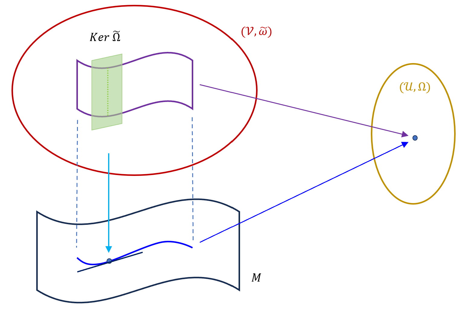
Figure 2: Souriau’s framework: the worldline in ${\bf M}$ is the projection of a characteristic sheet of the 2-form $\widetilde{\bf\Omega}={\bf d\tilde{{\bm{\omega}}}}$ on the evolution space, $\mathcal{V}$. Factoring out the characteristic foliation tangent to $\bf{\ker}\,\tilde{\mbox{\boldmath$\omega$}}$, $\mathcal{V}$ projects to the space of motions, $\mathcal{U}$, to which the 2-form $d\tilde{\omega}$ projects as a symplectic form ${\bf\Omega}$ and correspond to the worldlines in $M$.

Now we spell out a simplified form of the Souriau-Duval framework in flat space. For further details the reader is advised to consult DuvalAix79 ; DH82 .

$\bullet$ A massive free relativistic particle. The Poincaré group ($P$) is a fiber bundle over Minkowski spacetime $M$ with the Lorentz group as structure group Kunzle72 ; DuvalAix79 . We represent the Poincaré group by $5\times 5$ matrices ${\left(\begin{array}[]{ll}L&x\\ 0&1\end{array}\right)}$ where the $4\times 4$ matrix $L$ belongs to the Lorentz subgroup and $x=(x^{\mu})\in M$. Then

$$\text{Poincar\'{e}}/\text{Lorentz}=M=\text{Minkowski}\,.$$ (II.22)

Moreover, we choose the basepoint $Q_{m}$ in the Poincaré Lie algebra,

$$Q_{m}=\left(\begin{array}[]{cc}0&x_{m}\\ 0&0\end{array}\right){\quad\text{\small with}\quad}x_{m}=m{\tiny\left(\begin{array}[]{l}0\\ \vdots\\ 1\end{array}\right)}\in M$$ (II.23)

where $m=\mathop{\rm const}\nolimits$ interpreted as rest mass. Writing the Maurer-Cartan form as

$$g^{-1}dg=\left(\begin{array}[]{cc}L^{-1}dL&L^{-1}dx\\ 0&0\end{array}\right)$$ (II.24)

we get, on the Poincaré orbit ${\mathcal{O}}_{m}$ of $Q_{m}$,

$${\tilde{\omega}}_{m}=mI_{\mu}dx^{\mu}{\quad\Rightarrow\quad}{\tilde{\Omega}}_{m}=mdI_{\mu}\wedge dx^{\mu}\,$$ (II.25)

where $I_{\mu}$, a component of the Lorenz matrix, is future pointing and belongs to the unit tangent bundle of $M$ Kunzle72 ; DuvalAix79 ; DH82 . Then the characteristic foliation projects, in a suitable parametrisation, to $M$ onto a curve, which is a solution of

$$\dot{x}^{\mu}=I^{\mu},\qquad\dot{I}^{\mu}=0\,.$$ (II.26)

Eqn. (II.26) describes the geodesic motion in Minkowski space —  i.e.,  the motion of a free relativistic particle with no spin .

$\bullet$ The free theory based on the Poincaré group $P$ is readily extended to a (still free) relativistic particle with internal structure: enlarging the evolution space and 1-form, $P$ and ${\tilde{\omega}}_{m}$, respectively, to

$$\mathfrak{P}=P\times G{\quad\text{\small and}\quad}\omega={\tilde{\omega}}_{m}+Q_{0}\cdot g^{-1}dg\,,$$ (II.27)

where $g$ takes its values in the gauge group $G$ and the basepoint is $Q_{0}\in\mathfrak{G}$ (the Poincaré part being understood).

The kernel of $\tilde{\Omega}$ in (II.21) implies the free equation (II.26), supplemented by that for the isospin, (II.19), whose properties will be further studied in sec. III. In geometric language, the isospin belongs to the associated bundle $\mathfrak{P}\times_{G}{\mathcal{O}}_{0}$, where ${\mathcal{O}}_{0}$ is the (co)adjoint orbit of $Q_{0}$ in $\mathfrak{G}$. In local coordinates, $\mathfrak{P}\times_{G}{\mathcal{O}}_{0}\simeq M\times{\mathcal{O}}_{0}\,$ DH82 . The space of motions is ${\mathcal{O}}_{m}\times{\mathcal{O}}_{0}$ endowed with the projection of $\tilde{\Omega}$ in (II.21).

For $G=$ U$(1)$ the free charged particle is recovered, with $Q$ identified with the constant electric charge.

$\bullet$ minimal coupling to a Yang-Mills field amounts, in bundle language, to generalize (II.27) on $\mathfrak{P}$ by,

$$\omega={\tilde{\omega}}_{m}+Q_{0}\cdot\alpha\,,$$ (II.28)

with $Q_{0}\in\mathfrak{G}$, which, in view of (II.20), is indeed the geometric form of (II.5). In local coordinates,

$$\omega=\big{(}{\partial}_{\mu}+Q_{0}\cdot A_{\mu}\big{)}dx^{\mu}+Q_{0}\cdot g^{-1}dg\,.$$ (II.29)

The 2-form $\Omega=d\omega$ is, by the Cartan structure equations Kobayashi , p.78,

$$\Omega=\Omega_{0}+Q_{0}\cdot d\alpha=\Omega_{0}+Q_{0}\cdot\big{(}D\alpha-[\alpha,\alpha]\big{)}\,,$$ (II.30)

where the last term involves, in addition to the Lie bracket, also the wedge product of the differential forms. Its kernel projects to the Kerner-Wong equations (II.17)-(II.18) DH82 .

III Physical meaning of isospin dynamics

Limiting our investigations to flat Minkowski space, the Kerner equations (II.17) simplify to,

$$\ddot{x}_{\mu}=Q^{a}{\,}F_{\mu\nu}^{a}\,\dot{x}^{\nu}\,,$$ (III.1)

supplemented by the isospin equation (II.18) .

To what extent is the isospin vector, ${Q}$, an analog of the constant electric charge ? We argue that ${Q}=\mathop{\rm const}\nolimits$ would be inconsistent with gauge invariance: if we had $\dot{Q}=0$, the rhs of (II.18) would change, under a gauge transformation, as,

$$0=[{Q},A_{\mu}\dot{x}^{\mu}]\to[{Q},(g^{-1}A_{\mu}g)\dot{x}^{\mu}]+[{Q},(g^{-1}{\partial}_{\mu}g)\dot{x}^{\mu}]\,,$$

and there is no reason for the rhs to vanish. The situation improves, though, if the gauge transformation is non-trivially implemented on the isospin ,

$${Q}\to g^{-1}{Q}\,g\,.$$ (III.2)

Then the rhs of (II.18) would transform as

$$[{Q},A_{\mu}\dot{x}^{\mu}]\to g^{-1}\Big{\{}[{Q},A_{\mu}\dot{x}^{\mu}]+\left({Q}{\partial}_{\mu}g\,g^{-1}-{\partial}_{\mu}g\,g^{-1}{Q}\right)\dot{x}^{\mu}\Big{\}}\,g\,.$$

The first term in the curly bracket would be perfect but the 2nd one would vanish only for $g=\mathop{\rm const}\nolimits$. However the terms coming from $d(g^{-1}{Q}\,g)/ds$ cancel the unwanted terms, leaving us with the desired covariant transformation law cf. (III.2),

$$D_{s}{Q}\to g^{-1}D_{s}{Q}\,g\,.$$ (III.3)

Further insight into isospin dynamics can be gained by assuming, for simplicity, that the curvature of the connection form (in physical terms, the Yang-Mills field) is zero, $F=D\alpha=0$ which is a gauge-independent statement by (II.3), and the space-time motion is free. Do we have also $\dot{Q}=0\;?$ The answer is: yes and no. Let us explain. In topologically trivial situations , $F=D\alpha=0$ implies that one can find a gauge where $A_{\mu}=0$ and then $\dot{Q}=0$ follows obviously from the isospin equation (II.18). This is a gauge-dependent statement, though : We are allowed to apply a gauge transformation by an arbitrary $G=\mathrm{SU}(2)$-valued function $g(x^{\mu})$ which changes $A_{\mu}=0$ to a pure gauge $A_{\mu}=g^{-1}{\partial}_{\mu}g$ – but it rotates also the isospin, (III.2). $d{\big{(}g^{-1}{Q}\,g\big{)}/ds}\neq 0$ in general; the gauge-covariant statement is that the isospin is covariantly conserved, (II.19).

What is then the physical meaning of the isospin vector ? First we note that

$$|Q|^{2}=Q^{a}Q^{a}$$ (III.4)

is gauge invariant, and deriving it implies, using (III.3), that the length $|{Q}|$ is conserved,

$$\frac{d|{Q}|}{ds}=0{\quad\Rightarrow\quad}|{Q}|=\mathop{\rm const}\nolimits.$$ (III.5)

The isospin is thus constrained to lie on an adjoint orbit of the gauge group $G$ in its Lie algebra $\mathfrak{G}$ – in our case, to a sphere, ${Q}\in{\mathcal{O}}=\Big{\{}g^{-1}Q_{0}g\,\Big{|}\,g\in\mathrm{SU}(2)\Big{\}}\approx{\mathds{S}}^{2}\,.$ It is this fact that is behind the Souriau-type construction of isospin-extended models DuvalAix79 ; DH82 ; HP-Kollar .

Which components of ${Q}$ do have a gauge invariant physical meaning ? – the question leads to the so-called “color problem” NelsonMano83 ; MarmoBala82 ; NelsonColeman84 . The point is the subtle difference between gauge transformations and internal symmetries HRawnsley ; HRcolor .

In physical terms: can we implement an element of the gauge group on the physical fields ? And if we can, will it be a symmetry in the usual sense ForgacsManton ? In bundle language, a gauge transformation acts on the fibers from the right Kobayashi , — while a symmetry should act from the left HRawnsley ; HRcolor . Can we transfer the right-action to a left action ? In geometric terms, “implementable” means that the $G=\mathrm{SU}(2)$ bundle ${\mathfrak{P}}$ should be reducible, and “symmetry” requires that the connection form $\alpha$ in (II.20) which represents the YM potential should also be reducible to the reduced bundle.

When the underlying topology is non-trivial (as non-Abelian monopoles GoddardOlive ), there can be an obstruction : global color can not be defined”, as it is put in refs. NelsonMano83 ; MarmoBala82 ; NelsonColeman84 . Another physical instance is provided by the Non-Abelian Aharonov-Bohm effect WuYang75 , for which there is no obstruction but there is an ambiguity of how it should be implemented EZH-NABA .

IV Conservation laws with Isospin

IV.1 van Holten’s covariant framework

The Hamiltonian of a point particle of unit mass carrying isospin $\vec{Q}=(Q^{a})$ which moves in a static YM field is,

$$H=\frac{1}{2}\left({\vec{p}}-{\vec{A}}^{a}Q^{a}\right)^{2}\,,$$ (IV.1)

where we scaled the coupling constant again equal to one. Defining the covariant Poisson bracket as vHolten ,

$$\big{\{}f,g\big{\}}=\,D_{j}f\,\frac{{\partial}g}{{\partial}\pi_{j}}-\frac{{\partial}f}{{\partial}\pi_{j}}\,D_{j}g+\;Q^{a}F_{jk}^{a}\frac{{\partial}f}{{\partial}\pi_{j}}\,\frac{{\partial}g}{{\partial}\pi_{k}}-f^{abc}\frac{{\partial}f}{{\partial}Q^{a}}\frac{{\partial}g}{{\partial}Q^{b}}\,Q^{c},$$ (IV.2)

where the $f^{abc}$ are the structure constants of the Lie algebra, and the covariant phase-space derivative is,

$$D_{i}f={\partial}_{i}f-f^{abc}Q^{a}A_{i}^{b}\frac{\partial f}{\partial Q^{c}}\,.$$ (IV.3)

The nonzero Poisson brackets are,

$$\left\{x_{i,}p_{j}\right\}=\delta_{ij},\text{ \ \ }\left\{Q^{a},Q^{b}\right\}=-f^{abc}Q^{c}\,.$$ (IV.4)

Then the Hamilton equations with ${\vec{\pi}}=\dot{{\bm{r}}}$,

$$\dot{x}_{i}=\big{\{}x_{i},H\big{\}},\qquad\dot{\pi}_{i}=\big{\{}\pi_{i},H\big{\}},\qquad\dot{Q}^{a}=\big{\{}Q^{a},H\big{\}}\,$$ (IV.5)

allow us to recover the flat-space Kerner-Wong equations,

$$\ddot{x}^{i}= \;Q^{a}F_{ij}^{a}\dot{x}^{j}=Q^{a}\varepsilon^{ijk}\dot{x}^{j}B_{a}^{k}\,,$$ (IV.6a)

$$\dot{Q}^{a}= \;f^{abc}\dot{x}^{i}A_{b}^{i}Q_{c}\,,$$ (IV.6b)

equivalent to (III.1) and (II.18).

Following van Holten vHolten ; vHolten2 ; vHolten3 ; HP-NGOME , constants of the motion can be sought for by expanding into powers of the covariant momentum,

$$q=C({{\bm{r}}})+C_{i}({{\bm{r}}})\,\pi_{i}+\frac{1}{2!}C_{ij}({{\bm{r}}})\,\pi_{i}\pi_{j}+\dots$$ (IV.7)

Skipping the Abelian case, we move directly to the non-Abelian one. Requiring $q$ to Poisson-commute with the Hamiltonian then yields a series of constraints, eqn. # (70) in vHolten .

$$\begin{array}[]{ll}D_{i}C=Q^{a}F_{ij}^{a}C_{j}\,,\\[3.0pt] D_{i}C_{k}+D_{j}C_{i}=Q^{a}\big{(}F_{ik}^{a}C_{kj}+F_{jk}^{a}C_{ki}\big{)}\,,\\[3.0pt] D_{i}C_{jk}+D_{j}C_{ki}+D_{k}C_{ij}=Q^{a}\big{(}F_{il}^{a}C_{ljk}+F_{jl}^{a}C_{lki}+F_{kl}^{a}C_{lij}\big{)}\,,\\ \qquad\qquad\vdots\qquad\qquad\qquad\qquad\qquad\qquad\qquad\vdots&\end{array}$$ (IV.8)

The expansion (IV.8) can be truncated at a finite order when the covariant Killing equation is satisfied at some order $n$. When we have a Killing tensor, $D_{(i_{1}}C_{i_{2}\dots i_{n})}=0\,,$ then we can set

$$C_{i_{1}\dots i_{p}}=0$$ (IV.9)

for all $p\geq n$, and find a constant of the motion of the polynomial form,

$$q=\sum_{k=0}^{p-1}\frac{1}{k!}C_{i_{1}\dots i_{k}}\pi_{i_{1}}\dots\pi_{i_{k}}\,$$ (IV.10)

vHolten . Referring to the literature for details vHolten ; vHolten2 ; vHolten3 ; HP-NGOME we mention that in the Abelian theory $\vec{Q}$ is just a constant identified with the electric charge.

The van Holten algorithm can be generalized by adding a static scalar potential which may depend also on the isospin. The Hamiltonian (IV.1) then becomes

$$H=\frac{1}{2}\pi_{i}^{2}+V\left(x^{i},Q^{a}\right)$$ (IV.11)

with equations of motion,

$$\ddot{x}^{i}=\, \,Q^{a}F_{ij}^{a}\dot{x}^{j}-D_{i}V\,,$$ (IV.12a)

$$\dot{Q}^{a}=\, \,f^{abc}\dot{x}^{i}A_{b}^{i}Q_{c}+f^{abc}Q^{b}\frac{\partial V}{\partial Q^{c}}\,.$$ (IV.12b)

Comparison with (IV.6) then shows that (IV.12a) picks up a covariant force term. Note also that when $V$ does depend on ${\vec{Q}}$ the isospin is not more parellel transported.

Generalizing (IV.7) to isospin-dependent coefficients,

$$q({{\bm{r}}},{\vec{Q}})=C({{\bm{r}}},{\vec{Q}})+C_{i}({{\bm{r}}},{\vec{Q}})\,\pi_{i}+\frac{1}{2!}C_{ij}({{\bm{r}}},{\vec{Q}})\,\pi_{i}\pi_{j}+\dots$$ (IV.13)

the constraints (IV.8) are also generalised HP-NGOME ,

$$\begin{array}[]{lll}\;C_{i}D_{i}V+\displaystyle{f^{abc}Q^{a}\frac{{\partial}C}{\partial Q^{b}}\frac{{\partial}V}{{\partial}Q^{c}}}=0\,,\\[12.0pt] D_{i}C=Q^{a}F^{a}_{ij}\,C_{j}+C_{ij}D_{j}V+\displaystyle{f^{abc}Q^{a}\frac{{\partial}C_{i}}{\partial Q^{b}}\frac{{\partial}V}{{\partial}Q^{c}}}\,,\\[10.0pt] D_{i}C_{j}+D_{j}C_{i}=Q^{a}(F^{a}_{ik}C_{kj}+F^{a}_{jk}C_{ki})+\;C_{ijk}D_{k}V+\displaystyle{f^{abc}Q^{a}\frac{{\partial}C_{ij}}{\partial Q^{b}}\frac{{\partial}V}{{\partial}Q^{c}}}\,,\\ \quad\qquad\vdots\qquad\qquad\quad\qquad\qquad\qquad\qquad\vdots&\end{array}$$ (IV.14)

New, gradient-in-$V$ terms thus arise even when the potential does not depend on the isospin, $V=V({{\bm{r}}})$. These terms play a rôle for self-dual Wu-Yang monopoles WuYang69 , and for diatoms MSW , as it will be seen in subsections IV.2 and IV.3, respectively.

1. When $C_{i}({{\bm{r}}})$ is a Killing vector then we have $p=2$ and the expansion can be reduced to a linear expression,

   $$q=C({{\bm{r}}})+C_{i}({{\bm{r}}})\,\pi_{i}\,,$$ (IV.15)

   allowing us to recover the conserved momentum and angular momentum vHolten . Focusing our attention at the latter, we choose a unit vector ${\vec{n}}$; then

   $${\vec{C}}={\vec{n}}\times{{\bm{r}}}\,$$ (IV.16)

   is a Killing vector for rotations around ${\vec{n}}$ and thus generates the conserved angular momentum, ${\vec{J}}$. van Holten’s recipe can be applied also to a Dirac monopole of charge $q=eg$, recovering the angular momentum vector

   $${\vec{J}}={{\bm{r}}}\times{\vec{\pi}}-q\,{\hat{{\bm{r}}}}\,,$$ (IV.17)

   which includes the celebrated radial “spin from isospin” term Hasi ; HP-NGOME .

2. Similarly, choosing again a unit vector ${\vec{n}}$,

   $$C_{ij}=2\delta_{ij}\,{\vec{n}}\cdot{{\bm{r}}}-(n_{i}x_{j}+n_{j}x_{i})$$ (IV.18)

   is a Killing tensor of order $2$ which generates the well-known Runge-Lenz vector of planetary motion, vHolten ; vHolten2 ; vHolten3 ; HP-NGOME ,

   $${\vec{K}}={\vec{\pi}}\times{{\vec{J}}}+\alpha\,{{\hat{{\bm{r}}}}}\,.$$ (IV.19)

   More generally, the framework applies also to the so-called “MIC-Zwanziger” system MIC ; Zwanziger68 , which combines a Dirac monopole of charge $q$ with an arbitrary $r^{-1}$ Newtonian and a fine-tuned inverse-square potential,

   $$V(r)=\frac{q^{2}}{2r^{2}}+\frac{\alpha}{r}\,.$$ (IV.20)

   The combined system generalizes the well-known dynamical O(4)/O(3,1) symmetry of planetary motion spanned by the angular momentum and the Runge-Lenz vector, ${\vec{J}}$ in (IV.17) and ${\vec{K}}$, respectively MIC ; Zwanziger68 . The relations

   $${\vec{J}}\cdot{\hat{{\bm{r}}}}=-q{\quad\text{\small and}\quad}\big{[}{\vec{K}}+\hbox{$\textstyle\frac{\alpha}{q}$}{\vec{J}}\big{]}\cdot{{\bm{r}}}={\vec{J}}^{2}-q^{2}$$ (IV.21)

   then imply that the motion is a conic section, as depicted in FIG.3.

   

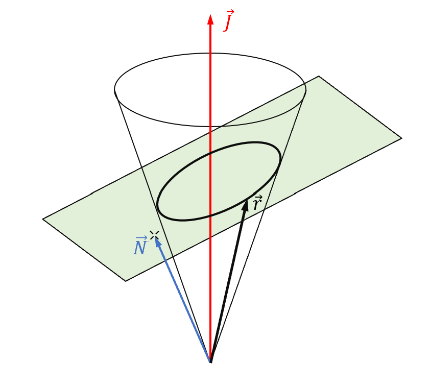
   Figure 3: The conservation of the monopole angular momentum ${\vec{J}}$ implies that a particle moves on a cone, whose axis is ${\vec{J}}$. The ${\rm O}(4)/{\rm O}(3,1)$ dynamical symmetry generated by the angular momentum and the Runge-Lenz vector ${\vec{K}}$ implies in turn that the trajectory lies in the plane perpendicular to ${\vec{N}}={\vec{K}}+(\alpha/q){\vec{J}}$ and is therefore a conic section.

   Spin can also be considered Feher:1988th .

   We mention that the MIC-Zwanziger system is essentially equivalent to the one which describes long-range monopole scattering GibbonsManton86 alias Kaluza-Klein monopole GrossPerry ; Sorkin See also FH86 ; Feher86 ; Feher87 ; Cordani88 ; CFH90 ; Feher:2009wwp ; MantonSutcliffe . The dynamical symmetry will be further analysed for a self-dual Wu-Yang monopole HWY in the next subsection.

3. The van Holten algorithm applies also to quantum dots, Hénon-Heiles and Holt systems, with Killing tensors whose rank ranges from one to six are studied in vHolten2 ; vHolten3 .

IV.2 Motion in the Wu-Yang monopole field

The Wu-Yang monopole WuYang69 is given by the non-Abelian gauge potential with a “hedgehog” magnetic field,

$$\displaystyle{A_{i}^{a}=\epsilon_{iak}\frac{x_{k}}{r^{2}}}\ ,\qquad F_{ij}^{a}=\epsilon_{ijk}\,\frac{x_{k}\;x_{a}}{r^{4}}\ .$$ (IV.22)

The terminology is justified by presenting the field strength as

$$B_{k}^{a}={\scriptstyle{\frac{1}{2}}}\epsilon_{ijk}F_{ij}^{a}=\frac{x^{k}x^{a}}{r^{4}}\,.$$ (IV.23)

The projection of the Wu-Yang magnetic field onto the “hedgehog” direction is thus

$$B_{k}^{a}\cdot\hat{x}^{a}=\dfrac{x^{k}}{r^{3}}\,,$$ (IV.24)

which shows that the Wu-Yang magnetic field is that of a Dirac monopole of unit charge, embedded into isospace. The remarkable feature of this expression is that the external and internal coordinates are correlated.

Let us consider an isospin-carrying particle moving in a Wu-Yang monopole field augmented with a rotationally invariant scalar potential $V(r)$, and inquire about conserved quantities.

$\bullet$ A most important observation says that, for an arbitrary radial potential $V(r)$, we can choose $C=\vec{Q}\cdot{\hat{{\bm{r}}}}$ which is covariantly constant,

$$D_{i}C=0.$$ (IV.25)

and the (IV.14) are satisfied with $C_{i}=C_{ij}=...=0$ . The van Holten algorithm then applies, proving that the projection of the isospin onto the radial direction,

$$q=C={\vec{Q}}\cdot{{\hat{{\bm{r}}}}}$$ (IV.26)

is a constant of the motion vHolten .

The Wu-Yang Ansatz (IV.22) played an important rôle in later developments as it prefigured the finite-energy non-Abelien monopoles tHooft ; Polyakov ; GoddardOlive . The “hedgehog” is the large-r behavior of the Higgs field, and (IV.26) is identified with the electric charge outside the monopole core. See e.g. GoddardOlive or MantonSutcliffe for comprehensive reviews.

$\bullet$ Applied to the Killing vector (IV.16), we get the conserved angular momentum vHolten ,

$${\vec{J}}={{\bm{r}}}\times{\vec{\pi}}-q\,{{\hat{{\bm{r}}}}}\;,$$ (IV.27)

which looks formally identical to the Abelian expression (IV.17). Remember however that $q$ here is not a universal constant but the (conserved) projection of the isospin onto the “hedgehog” direction ${\hat{{\bm{r}}}}$, which mixes internal and external coordinates. Thus we have the familiar radial term – but now in the non-Abelian context.

$\bullet$ We now inquire about quantities which are quadratic in the momentum. Inserting (IV.18) into (IV.14), from the 2nd-order equation we find,

$${\vec{C}}=\vec{n}\times(q\,{{\hat{{\bm{r}}}}})\;.$$ (IV.28)

For which potentials do we get a quadratic conserved quantity ? Referring to vHolten ; HP-NGOME for details, we just record the answer:

$$C=\alpha\;\vec{n}\cdot{{\hat{{\bm{r}}}}}{\quad\text{\small and}\quad}V(r)=\frac{q^{2}}{2r^{2}}+\frac{\alpha}{r}+\beta\,,$$ (IV.29)

where $\alpha$ and $\beta$ are arbitrary constants. The coefficient of the $r^{-2}$ term is correlated with the conserved charge $q$ (IV.26) as (IV.20) for MIC-Zwanziger MIC ; Zwanziger68 ; Feher87 . Collecting our results,

$${\vec{K}}={\vec{\pi}}\times{{\vec{J}}}+\alpha\,{{\hat{{\bm{r}}}}}\,,$$ (IV.30)

is a conserved Runge-Lenz vector for an isospin-carrying particle in the Wu-Yang monopole field combined with the fine-tuned potential $V(r)$ in (IV.29).

The conserved quantities ${\vec{J}}$ and ${\vec{K}}$ span an ${\rm O}(4)/{\rm O}(3,1)$ dynamical symmetry which allow us to describe the large-r motion both classically and quantum mechanically Feher86 ; Feher:1984xc . The trajectories are again conic sections as for MIC-Zwanziger in FIG.3.

This generalizes the Abelian result to an isospin-carrying particle outside the core of a self-dual non-Abelian monopole HWY . This “coincidence” is explained as follows : for large $r$, the gauge field of a self-dual non-Abelian monopole of charge $m$ GoddardOlive is of the radially symmetric Wu-Yang form, eqn. (IV.22), completed with a “hedgehog” Higgs field,

$$\Phi^{a}=\Big{(}1-\displaystyle\frac{m}{r}\Big{)}\,\displaystyle\frac{x^{a}}{r}\,,$$ (IV.31)

whose direction is, precisely,

$$\widehat{\Phi}=\frac{\Phi}{|\Phi|}={\hat{{\bm{r}}}}\,.$$ (IV.32)

The projection of the isospin onto $\widehat{\Phi}$, $q$ in (IV.26), is thus conserved, and outside the core the motion is that of an electric charge in the MIC-Zwanziger field MIC ; Zwanziger68 ; Feher:1984xc ; Feher86 ; Feher87 . The isospin-dependent dynamical symmetry is analyzed in HWY .

IV.3 Diatomic molecules

In Ref. MSW Moody, Shapere and Wilczek have shown that nuclear motion in a diatomic molecule can be described by the effective non-Abelian gauge field,

$${A}_{i}^{\;a}=(1-\kappa)\epsilon_{iaj}\,\frac{x_{j}}{r^{2}}{\quad\text{\small and}\quad}\displaystyle{{F}^{\;a}_{ij}=(1-\kappa^{2})\epsilon_{ijk}\frac{x_{k}x_{a}}{r^{4}}}\,,$$ (IV.33)

respectively, where $\kappa$ is a real parameter. For $\kappa=0$, (IV.33) is the field of the Wu-Yang monopole WuYang69 , (IV.22). For other values of $\kappa$, it is a truly non-Abelian configuration (except for $\kappa=\pm 1$, when the field strength vanishes and (IV.33) is a gauge transform of the vacuum).

Dropping scalar potential $V(r)$ we return to the Hamiltonian of a spinless particle with non-Abelian structure, (IV.1),

$$H={\scriptstyle{\frac{1}{2}}}{\vec{\pi}}^{2},\quad{\vec{\pi}}={\vec{p}}-{\vec{A}}\,.$$ (IV.34)

Inquiring about conserved quantities, we note first that when $\kappa\neq 0$, then $q$ is not covariantly conserved in general,

$$D_{j}q=\frac{\kappa}{r}\left(Q^{j}-q\frac{x_{j}}{r}\right)\neq 0\,,$$ (IV.35)

implying that $q$ in (IV.26) is not conserved for $\kappa\neq 0$,

$$\quad\big{\{}H,q\big{\}}=-{\vec{\pi}}\cdot{\vec{D}}q\neq 0\,.$$ (IV.36)

unless the isospin is also radial. The bracketed quantity in (IV.35) is indeed the non-aligned-with-the-field piece of the isospin. When the isospin spin and the magnetic field happen to be aligned, then $q$ in (IV.26) is conserved.

Nor is the length of the to-become-charge $q$ is conserved in general,

$$\big{\{}H,q^{2}\big{\}}=-2\kappa q\,({\vec{\pi}}\cdot{\vec{D}}q)\neq 0\,.$$ (IV.37)

whereas le the length of the isospin, $\vec{Q}^{2}$, is conserved, $\{H,\vec{Q}^{2}\}=0$. Thus electric charge non-conservation comes from isospin precession, as in the non-Abelian Aharonov-Bohm effect WuYang75 ; MSW ; EZH-NABA . For $\kappa=0$ we recover the Wu-Yang case when $q$ is conserved as we have seen in sec.IV.2.

The gauge field (IV.33) is rotationally symmetric and an isospin-carrying particle submitted to it has, nevertheless conserved angular momentum MSW ; Jackiw86 . Its form is, however, somewhat unconventional.

Our starting point is the first-order condition in (IV.14). We consider first $V=0$ ; then with $F_{jk}^{a}$ in (IV.33), the equation to be solved is

$$D_{i}C=(1-\kappa^{2})\,\frac{q}{r}\,\left(({\vec{n}}\cdot{\hat{{\bm{r}}}})\frac{x_{i}}{r}-n_{i}\right).$$ (IV.38)

In the Wu-Yang case, $\kappa=0$, we have $C=-{\vec{n}}\,\cdot\,q\,{{\hat{{\bm{r}}}}}$, but for $\kappa\neq 0$ the to-be electric charge, $q$, is not conserved. Using (IV.36) allows us to infer HP-NGOME that

$$C=-{\vec{n}}\cdot\Big{(}q\,{{\hat{{\bm{r}}}}}+\kappa({\vec{Q}}-q{\hat{{\bm{r}}}})\Big{)}\,.$$ (IV.39)

The conserved angular momentum is, therefore,

$${\vec{J}} = {{\bm{r}}}\times{\vec{\pi}}-{\vec{\Psi}},$$ (IV.40)

$${\vec{\Psi}} = q\,{{\hat{{\bm{r}}}}}+\kappa\,({\vec{Q}}-q{\hat{{\bm{r}}}})=q\,{\hat{{\bm{r}}}}+\kappa\,\big{(}{\hat{{\bm{r}}}}\times{\vec{Q}}\big{)}\times{\hat{{\bm{r}}}},$$ (IV.41)

consistently with the results in MSW ; Jackiw86 . Note however that the spin-from-isospin contribution changes, w.r.t. (IV.27),

$$q\,{\hat{{\bm{r}}}}\to{\vec{\Psi}}\,.$$ (IV.42)

For $\kappa=0$ we recover the Wu-Yang expression, (IV.27). Eliminating ${\vec{\pi}}$ in favor of ${\vec{p}}={\vec{\pi}}+{\vec{A}}$ allows us to rewrite the total angular momentum as

$${\vec{J}}={{\bm{r}}}\times{\vec{p}}-{\vec{Q}}\,,$$ (IV.43)

making manifest the “spin from isospin term” which is however not aligned with the “hedgehog” magnetic field. Consistently with (IV.35), the non-conservation of $q$ in (IV.26) comes precisely for this non-alignement.

Restoring the potential, we see that, again due to the non-conservation of $q$, $D_{j}V\neq 0$ in general. The zeroth-order condition ${\vec{C}}\cdot{\vec{D}}V=0$ in (IV.14) is nevertheless satisfied if $V$ is a radial function which is independent of ${\vec{Q}}$, $V=V(r)$, since then ${\vec{D}}V=\vec{\nabla}V$, which is perpendicular to infinitesimal rotations, ${\vec{C}}$. Alternatively, a direct calculation, using the same formulae allow us to confirm that ${\vec{J}}$ commutes with the Hamiltonian, $\{J_{i},H\}=0$.

Multiplying (IV.43) by ${\hat{{\bm{r}}}}$ yields by, once again,

$${\vec{J}}\cdot{\hat{{\bm{r}}}}=-q$$ (IV.44)

as in the Wu-Yang case. This is, however, less useful as before, since $q$ is not a constant of the motion anymore so that the angle between ${\vec{J}}$ and the radius vector, ${{\bm{r}}}(t)$, is not constant either: the motion is not confined to a cone anymore.

Our attempts to find a conserved Runge-Lenz vector for the diatomic system have failed.

V Conclusion and outlook

The groundbreaking work of Kerner, Kerner68 and of Wong Wong70 , continued by many others, Trautman70 ; Cho75 ; Balachandran76 ; Balachandran77 ; Sternberg77 ; Sternberg78 ; Weinstein78 ; Sternberg80 ; DuvalCRAS ; DuvalAix79 ; DH82 ; Montgomery ; JackiwManton ; FeherAPH allow us to gain an insight into the structure of non-Abelian gauge theory YangMills . Our paper reviews the KK framework, retraces the chronological order of these discoveries and analyses the subtle physical meaning of isospin dynamics.

In addition to the conceptual works above, we underline that the Kerner-Wong model Kerner68 ; Wong70 admits important physical applications.

The analysis in a self-dual monopole field Feher86 ; Feher87 ; Feher:1988th ; CFH90 could be paralleled by studying motion in pure YM configurations with no scalar field Schechter ; Wipf and also monopole scattering GibbonsManton86 ; FH86 ; Cordani88 ; CFH90 ; Feher:2009wwp alias Kaluza-Klein monopole GrossPerry ; Cordani88 ; Sorkin .

In sec.IV we applied van Holten’s algorithm vHolten ; vHolten2 ; vHolten3 ; HP-NGOME conservation laws for a particle with isospin in non-Abelian fields examplified by a Wu-Yang monopole WuYang69 ; vHolten , and of diatomic molecules MSW ; Jackiw86 ; HP-NGOME . The O(4)/O(3,1) dynamical symmetry of a Wu-Yang monopole augmented with a self-dual Higgs field and implying elliptic trajectories is broken for diatomic molecules due to the non-conservation of the to-become electric charge, $q$ in (IV.26).

- (1) R. Kerner, “Generalization of the Kaluza-Klein Theory for an Arbitrary Nonabelian Gauge Group,” Ann. Inst. H. Poincare Phys. Theor. 9 (1968), 143-152
- (2) S. K. Wong, “Field and particle equations for the classical Yang-Mills field and particles with isotopic spin,” Nuovo Cimento 65A, 689 (1970)
- (3) A. Trautman, “Fiber bundles associated with space-time,” Rept. Math. Phys. 1 (1970), 29-62 doi:10.1016/0034-4877(70)90003-0
- (4) Y. M. Cho, “Higher - Dimensional Unifications of Gravitation and Gauge Theories,” J. Math. Phys. 16 (1975), 2029 doi:10.1063/1.522434
- (5) A. P. Balachandran, P. Salomonson, B. S. Skagerstam and J. O. Winnberg, “Classical Description of Particle Interacting with Nonabelian Gauge Field,” Phys. Rev. D 15 (1977), 2308-2317 doi:10.1103/PhysRevD.15.2308
- (6) A. P. Balachandran, S. Borchardt and A. Stern, “Lagrangian and Hamiltonian Descriptions of Yang-Mills Particles,” Phys. Rev. D 17 (1978), 3247 doi:10.1103/PhysRevD.17.3247
- (7) S. Sternberg, “Minimal Coupling and the Symplectic Mechanics of a Classical Particle in the Presence of a Yang-Mills Field,” Proc. Nat. Acad. Sci. 74 (1977), 5253-5254 doi:10.1073/pnas.74.12.5253
- (8) V. Guillemin and S. Sternberg, “On the Equations of Motion of a Classical Particle in a Yang-Mills Field and the Principle of General Covariance,” Hadronic J. 1 (1978), 1 TAUP-655-78.
- (9) S. Sternberg, “On the role of field theories in our physical conception of geometry,” 2nd Bonn Conference on Diff. Geom. Meths. in Math. Phys., Lecture Notes in Math. 676, Springer (Berlin 1980) pp. 1-88.
- (10) A. Weinstein, “A Universal Phase Space for Particles in Yang-Mills Field,” Lett. Math. Phys. 2 (1978), 417-420 doi:10.1007/BF00400169
- (11) C. Duval, “Sur les mouvements classiques dans un champs de Yang-Mills,” Unpublished Marseille preprint CPT-78-P-1056
- (12) C. Duval, “On the prequantum description of spinning particles in an external gauge field,” Proc. Aix Conference on Diff. Geom. Meths. in Math. Phys. Ed. Souriau. Springer LNM 836, 49-67 (1980). This comprehensive paper is indeed the extended version of Duval’s DuvalCRAS .
- (13) C. Duval and P. A. Horvathy, “Particles with internal structure: the geometry of classical motions and conservation laws.” Ann. Phys. (N.Y.) 142, 10 (1982).
- (14) R. Montgomery, “CANONICAL FORMULATIONS OF A CLASSICAL PARTICLE IN A YANG-MILLS FIELD AND WONG’S EQUATIONS,” Lett. Math. Phys. 8 (1984), 59-67 doi:10.1007/BF00420042
- (15) L. G. Fehér, “Classical motion of coloured test particles along geodesics of a Kaluza-Klein spacetime,” Acta Phys. Hung. 59 (1986), 437-444
- (16) R. Jackiw and N. S. Manton, “Symmetries And Conservation Laws In Gauge Theories,” Annals Phys. 127 (1980) 257.
- (17) G. ’t Hooft, “Magnetic monopoes in unified gauge theories,” Nucl. Phys. B79 (1974) 276 https://doi.org/10.1016/0550-3213(74)90486-6
- (18) A. M. Polyakov, “Particle Spectrum in Quantum Field Theory,” JETP Lett. 20 (1974), 194-195 PRINT-74-1566 (LANDAU-INST).
- (19) P. Goddard and D. I. Olive, “New Developments in the Theory of Magnetic Monopoles,” Rept. Prog. Phys. 41 (1978), 1357 doi:10.1088/0034-4885/41/9/001
- (20) L. G. Fehér, “Bounded Orbits for Classical Motion of Colored Test Particles in the Prasad-Sommerfield Monopole Field,” Acta Phys. Polon. B 15 (1984), 919 Print-84-0247 (BOLYAI).
- (21) L. G. Fehér, “Quantum Mechanical Treatment of an Isospinor Scalar in Yang-Mills Higgs Monopole Background,” Acta Phys. Polon. B 16 (1985), 217 PRINT-84-0552 (BOLYAI-INST).
- (22) L. G. Fehér, “Dynamical O(4) Symmetry in the Asymptotic Field of the Prasad-sommerfield Monopole,” J. Phys. A 19 (1986), 1259-1270 doi:10.1088/0305-4470/19/7/026
- (23) L. G. Fehér and P. A. Horvathy, “Non-relativistic scattering of a spin-1/2 particle off a self-dual monopole,” Mod. Phys. Lett. A 3 (1988), 1451-1460 doi:10.1142/S0217732388001744 [arXiv:0903.0249 [hep-th]]
- (24) T. T. Wu and C. N. Yang, “Concept of Nonintegrable Phase Factors and Global Formulation of Gauge Fields,” Phys. Rev. D 12 (1975), 3845-3857 doi:10.1103/PhysRevD.12.3845 see also WY76 below.
- (25) T. T. Wu and C. N. Yang, “Dirac’s Monopole Without Strings: Classical Lagrangian Theory,” Phys. Rev. D 14 (1976), 437-445 doi:10.1103/PhysRevD.14.437
- (26) P. A. Horvathy, “The Nonabelian Aharonov-Bohm Effect,” Phys. Rev. D 33 (1986), 407-414 doi:10.1103/PhysRevD.33.407. A preliminary version is P. A. Horvathy, “THE NONABELIAN AHARONOV-BOHM EFFECT,” BI-TP-82/14.
- (27) C. N. Yang and R. L. Mills, “Conservation of Isotopic Spin and Isotopic Gauge Invariance,” Phys. Rev. 96 (1954), 191-195 doi:10.1103/PhysRev.96.191
- (28) M. Elbistan, P-M. Zhang and P.A. Horvathy, “Isospin precession in the non-Abelian Aharonov-Bohm scattering,” (work in progress).
- (29) M. G. Alford, J. March-Russell and F. Wilczek, “Discrete Quantum Hair on Black Holes and the Nonabelian Aharonov-Bohm Effect,” Nucl. Phys. B 337 (1990), 695-708 doi:10.1016/0550-3213(90)90512-C
- (30) J. Preskill and L. M. Krauss, “Local Discrete Symmetry and Quantum Mechanical Hair,” Nucl. Phys. B 341 (1990), 50-100 doi:10.1016/0550-3213(90)90262-C
- (31) R. H. Brandenberger, “Topological defects and structure formation,” Int. J. Mod. Phys. A 9 (1994), 2117-2190 doi:10.1142/S0217751X9400090X [arXiv:astro-ph/9310041 [astro-ph]].
- (32) K. Osterloh, M. Baig, L. Santos, P. Zoller, and M. Lewenstein, “Cold Atoms in Non-Abelian Gauge Potentials: From the Hofstadter ”Moth” to Lattice Gauge Theory,” Phys. Rev. Lett. 95, 010403 (2005).
- (33) N. Goldman, G. Juzeliūnas, P. Öhberg and I. B. Spielman, “Light-induced gauge fields for ultracold atoms,” Rept. Prog. Phys. 77 (2014) no.12, 126401 doi:10.1088/0034-4885/77/12/126401 [arXiv:1308.6533 [cond-mat.quant-gas]].
- (34) A. Jacob, P. Öhberg, G. Juzeliūnas, and L. Santos, “Cold atom dynamics in non-Abelian gauge fields,” Appl. Phys. B 89, 439 (2007).
- (35) J. Dalibard, F. Gerbier, G. Juzeliūnas, P. Öhberg, “Colloquium: Artificial gauge potentials for neutral atoms,” Rev. Mod. Phys. 83, 1523-1543 (2011).
- (36) Y. Chen, R. Y. Zhang, Z. Xiong, Z. H. Hang, J. Li, J. Q. Shen and C. T. Chan, “Non-Abelian gauge field optics,” Nature Commun. 10 (2019) no.1, 3125 doi:10.1038/s41467-019-10974-8 [arXiv:1802.09866 [physics.optics]].
- (37) Y. Yang, C. Peng, D. Zhu, H. Buljan, J. D. Joannopoulos, B. Zhen and M. Soljačić, “Synthesis and Observation of Non-Abelian Gauge Fields in Real Space,” Science 365 (2019), 1021 doi:10.1126/science.aay3183 [arXiv:1906.03369 [physics.optics]].
- (38) J. Wu, Z. Wang, Y. Biao, F. Fei, S. Zhang, Z. Yin, Y. Hu, Z. Song, T. Wu, F. Song, et al., “Non-Abelian gauge fields in circuit systems,” Nature Electronics 5, 635 (2022)
- (39) R. Németh and J. Cserti, “Differential scattering cross section of the non-Abelian Aharonov-Bohm effect in multiband systems,” Phys. Rev. B 108 (2023) no.15, 155402 doi:10.1103/PhysRevB.108.155402 [arXiv:2306.13448 [quant-ph]].
- (40) T. T. Wu and C. N. Yang, “Some solutions of the classical isotopic gauge field equations,” in Properties of Matter under Unusual Conditions. Festschrift for the 60th birthday of E. Teller. p. 349. Ed. H. Mark and S. Fernbach. Interscience: (1969).
- (41) J. Moody, A. Shapere, and F. Wilczek, “Realization of magnetic monopole gauge fields : diatoms and spin precession,” Phys. Rev. Lett. 56, 893 (1986)
- (42) R. Jackiw, “Angular momentum for diatoms described by gauge fields” Phys. Rev. Lett. 56, 2779 (1986).
- (43) W. Heisenberg, “On the structure of atomic nuclei,” Z. Phys. 77 (1932), 1-11 doi:10.1007/BF01342433
- (44) L. O’Raifeartaigh, “The dawning of gauge theory,” Princeton Univ. Press, 1997, ISBN 978-0-691-02977-1
- (45) E. S. Abers and B. W. Lee, “Gauge Theories,” Phys. Rept. 9 (1973), 1-141 doi:10.1016/0370-1573(73)90027-6
- (46) T. Kaluza, “Zum Unitätsproblem der Physik,” Sitzungsber. Preuss. Akad. Wiss. Berlin (Math. Phys.) 1921 (1921), 966-972 doi:10.1142/S0218271818700017 [arXiv:1803.08616 [physics.hist-ph]]. [english translation: On the Unification Problem in Physics]. Contribution to: International School of Cosmology and Gravitation: 8th Course: Unified Field Theories of More than Four Dimensions, Including Exact Solutions e-Print: 1803.08616 [physics.hist-ph]
- (47) O. Klein, “Quantentheorie und fünfdimensionale Relativitätstheorie,” [“Quantum Theory and Five-Dimensional Theory of Relativity]. (In German and English),” Z. Phys. 37 (1926), 895-906 doi:10.1007/BF01397481 Contribution to: International School of Cosmology and Gravitation: 8th Course: Unified Field Theories of More than Four Dimensions, Including Exact Solutions.
- (48) D. J. Gross and M. J. Perry, “Magnetic Monopoles in Kaluza-Klein Theories,” Nucl. Phys. B 226 (1983), 29-48 doi:10.1016/0550-3213(83)90462-5
- (49) H. Arodz, “Colored, Spinning Classical Particle in an External Nonabelian Gauge Field,” Phys. Lett. B 116 (1982), 251-254 doi:10.1016/0370-2693(82)90336-7; “A Remark on the Classical Mechanics of Colored Particles,” Phys. Lett. B 116 (1982), 255-258 “LIMITATION OF THE CONCEPT OF THE CLASSICAL COLORED PARTICLE,” Acta Phys. Polon. B 14 (1983), 13-21
- (50) P. A. Horvathy and J. H. Rawnsley, “Internal Symmetries of Nonabelian Gauge Field Configurations,” Phys. Rev. D 32 (1985), 968 doi:10.1103/PhysRevD.32.968 ;
- (51) P. A. Horvathy and J. H. Rawnsley, “The Problem of ’Global Color’ in Gauge Theories,” J. Math. Phys. 27 (1986), 982 doi:10.1063/1.527119
- (52) J.-M. Souriau, Structure des systèmes dynamiques, Dunod (1970). Structure of Dynamical Systems. A Symplectic View of Physics, Birkhäuser, Boston (1997).
- (53) H V McIntosh and A. Cisneros, “Degeneracy in the Presence of a Magnetic Monopole,” J. Math. Phys. 11, 896-916 (1970) https://doi.org/10.1063/1.1665227.
- (54) D. Zwanziger, “Exactly soluble nonrelativistic model of particles with both electric and magnetic charges,” Phys. Rev. 176 (1968), 1480-1488 doi:10.1103/PhysRev.176.1480
- (55) S. Kobayashi and K. Nomizu, Foundations of Differential Geometry Vols. I and II, (Interscience, New York, 1963 and 1969)
- (56) C. N. Yang, “FIBER BUNDLES AND THE PHYSICS OF THE MAGNETIC MONOPOLE,” CERN-TH-2725.
- (57) A. P. Balachandran, G. Marmo and A. Stern, “Magnetic Monopoles With No Strings,” Nucl. Phys. B 162 (1980), 385-396 doi:10.1016/0550-3213(80)90346-6
- (58) P. A. Horvathy, “Classical Action, the Wu-Yang Phase Factor and Prequantization,” Lect. Notes Math. 836 (1980), 67-90 doi:10.1007/BFb0089727
- (59) H. P. Künzle, “Canonical Dynamics of Spinning Particles in Gravitational and Electromagnetic Fields,” J. Math. Phys. 13, (1972), 739.
- (60) P. C. Nelson and A. Manohar, “Global Color Is Not Always Defined,” Phys. Rev. Lett. 50 (1983), 943 doi:10.1103/PhysRevLett.50.943
- (61) A. P. Balachandran, G. Marmo, N. Mukunda, J. S. Nilsson, E. C. G. Sudarshan and F. Zaccaria, “Monopole Topology and the Problem of Color,” Phys. Rev. Lett. 50 (1983), 1553 doi:10.1103/PhysRevLett.50.1553
- (62) P. C. Nelson and S. R. Coleman, “What Becomes of Global Color,” Nucl. Phys. B 237 (1984), 1-31 doi:10.1016/0550-3213(84)90013-0
- (63) P. A. Horvathy and J. Kollar, “The Nonabelian Aharonov-Bohm Effect in Geometric Quantization,” Class. Quant. Grav. 1 (1984), L61 doi:10.1088/0264-9381/1/6/002
- (64) P. A. Horvathy, “THE WU-YANG FACTOR AND THE NONABELIAN AHARONOV-BOHM EXPERIMENT,” EPL 2 (1986), 195 doi:10.1209/0295-5075/2/3/005
- (65) P. Forgács and N. S. Manton, “Space-Time Symmetries in Gauge Theories,” Commun. Math. Phys. 72 (1980), 15 doi:10.1007/BF01200108
- (66) J. Schechter, “Yang-Mills particle in ’t Hooft’s gauge field,” Phys. Rev. D14, 524 (1976)
- (67) A. Wipf, “Nonrelativistic Yang-Mills particle in a spherically symmetric monopole field,” J. Phys. A18, 2379 (1985).
- (68) J. W. van Holten, “Covariant Hamiltonian dynamics,” Phys. Rev. D 75 (2007), 025027 doi:10.1103/PhysRevD.75.025027 [arXiv:hep-th/0612216 [hep-th]].
- (69) P. A. Horvathy and J. P. Ngome, “Conserved quantities in non-abelian monopole fields,” Phys. Rev. D 79 (2009), 127701 doi:10.1103/PhysRevD.79.127701 [arXiv:0902.0273 [hep-th]].
- (70) M. Cariglia, G. W. Gibbons, J. W. van Holten, P. A. Horvathy, P. Kosinski and P. M. Zhang, “Killing tensors and canonical geometry,” Class. Quant. Grav. 31 (2014), 125001 doi:10.1088/0264-9381/31/12/125001 [arXiv:1401.8195 [hep-th]].
- (71) M. Cariglia, G. W. Gibbons, J. W. van Holten, P. A. Horvathy and P. M. Zhang, “Conformal Killing Tensors and covariant Hamiltonian Dynamics,” J. Math. Phys. 55 (2014), 122702 doi:10.1063/1.4902933 [arXiv:1404.3422 [math-ph]].
- (72) P. Hasenfratz and G. ’t Hooft, “A Fermion-Boson Puzzle in a Gauge Theory,” Phys. Rev. Lett. 36 (1976), 1119 doi:10.1103/PhysRevLett.36.1119
- (73) G. W. Gibbons and N. S. Manton, “Classical and Quantum Dynamics of BPS Monopoles,” Nucl. Phys. B 274 (1986), 183-224 doi:10.1016/0550-3213(86)90624-3
- (74) L. G. Feher and P. A. Horvathy, “Dynamical Symmetry of Monopole Scattering,” Phys. Lett. B 183 (1987), 182 [erratum: Phys. Lett. B 188 (1987), 512] doi:10.1016/0370-2693(87)90435-7
- (75) B. Cordani, L. G. Feher and P. A. Horvathy, “O(4,2) Dynamical Symmetry of the Kaluza-Klein Monopole,” Phys. Lett. B 201 (1988), 481-486 doi:10.1016/0370-2693(88)90604-1
- (76) B. Cordani, L. G. Feher and P. A. Horvathy, “Kepler Type Dynamical Symmetries of Long Range Monopole Interactions,” J. Math. Phys. 31 (1990), 202 doi:10.1063/1.528862
- (77) R. d. Sorkin, “Kaluza-Klein Monopole,” Phys. Rev. Lett. 51 (1983), 87-90 doi:10.1103/PhysRevLett.51.87
- (78) L. G. Feher, “The O(3,1) Symmetry Problem of the Charge - Monopole Interaction,” J. Math. Phys. 28 (1987), 234-239 doi:10.1063/1.527802
- (79) L. G. Feher and P. A. Horvathy, “Dynamical symmetry of the Kaluza-Klein monopole,” [arXiv:0902.4600 [hep-th]]. arXiv: hep-th/0612216.
- (80) N. S. Manton and P. Sutcliffe, “Topological solitons,” Cambridge University Press, 2004, ISBN 978-0-521-04096-9, 978-0-521-83836-8, 978-0-511-20783-9 doi:10.1017/CBO9780511617034
- (81) P. A. Horvathy, “Isospin dependent O(4,2) symmetry of selfdual Wu-Yang monopoles,” Mod. Phys. Lett. A 6 (1991), 3613-3620 doi:10.1142/S0217732391004164