Rank and Select on Degenerate Strings
Abstract
A degenerate string is a sequence of subsets of some alphabet; it represents any string obtainable by selecting one character from each set from left to right. Recently, Alanko et al. generalized the rank-select problem to degenerate strings, where given a character c and position i the goal is to find either the ith set containing c or the number of occurrences of c in the first i sets [SEA 2023]. The problem has applications to pangenomics; in another work by Alanko et al. they use it as the basis for a compact representation of de Bruijn Graphs that supports fast membership queries.
In this paper we revisit the rank-select problem on degenerate strings, introducing a new, natural parameter and reanalyzing existing reductions to rank-select on regular strings. Plugging in standard data structures, the time bounds for queries are improved exponentially while essentially matching, or improving, the space bounds. Furthermore, we provide a lower bound on space that shows that the reductions lead to succinct data structures in a wide range of cases. Finally, we provide implementations; our most compact structure matches the space of the most compact structure of Alanko et al. while answering queries twice as fast. We also provide an implementation using modern vector processing features; it uses less than one percent more space than the most compact structure of Alanko et al. while supporting queries four to seven times faster, and has competitive query time with all the remaining structures.
1 Introduction
Given a string over an alphabet the rank-select problem is to preprocess to support, for any ,
-
•
: return the number of occurrences of in
-
•
: return the index of the th occurrence of in
This fundamental string problem has been studied extensively due to its wide applicability, see, e.g., [8, 26, 14, 28, 27, 7, 23, 11, 6, 5, 25, 18, 24, 17], references therein, and surveys [12].
A degenerate string is a sequence where each is a subset of . We define its length to be , its size to be , and denote by the number of empty sets among . Degenerate strings have been studied since the 80s [1] and the literature contains papers on problems such as degenerate string comparison [4], finding string covers for degenerate strings[10], and pattern matching with degenerate patterns, degenerate texts, or both [1, 19].
Alanko, Biagi, Puglisi, and Vuohtoniemi [2] recently generalized the rank-select problem to the subset rank-select problem, where the goal is to preprocess a given degenerate string to support
-
•
: return the number of sets in that contain
-
•
: return the index of the th set that contains
Their motivation for studying this problem is to support fast membership queries on de Bruijn graphs, a useful tool in pangenomic problems such as genome assembly and pangenomic read alignment (see [2, 3] for details and further references). Specifically, in another work by some of the authors [3], they show how to represent the de Bruijn graph of all length- substrings of a given string such that membership queries on the graph can be answered using subset-rank queries. They also provide an implementation that, when compared to the previous state of the art, improves query time by one order of magnitude while improving space usage, or by two orders of magnitude with similar space usage.
Their result for subset rank-select is the following [2]. They introduce the Subset Wavelet Tree, a generalization of the well-known wavelet tree (see [16]) to degenerate strings. It supports both subset-rank and subset-select queries in time and uses bits of space in the general case. In the special case of (which is the case for their representation of de Bruijn Graphs in [3]) they show that their structure uses bits. We note that their analysis for this special case happens to generalize nicely to also show that their structure uses at most bits for any .
Furthermore, in [3], Alanko, Puglisi, and Vuohtoniemi present a number of reductions from the subset rank-select to the regular rank-select problem. We will elaborate on these reductions later in the paper.
2 Our Results
Our contributions are threefold. Firstly, we introduce the natural parameter and revisit the subset rank-select problem to reanalyze a number of simple and elegant reductions to the regular rank-select problem, based on the reductions from [3]. We express the complexities in terms of the performance of a given rank-select structure, achieving flexible bounds that benefit from the rich literature on the rank-select problem (Theorem 1). Secondly, we show that any structure supporting either subset-rank or subset-select must use at least bits in the worst case (Theorem 2). By plugging a standard rank-select data structure into Theorem 1 we, in many cases, match this bound to within lower order terms, while simultaneously matching the query time of the fastest known rank-select data structures (see below). Note that any lower bound for rank-select queries also holds for subset rank-select queries since any string is also a degenerate string. All our results hold on a word RAM with logarithmic word-size. Finally, we provide implementations of the reductions and compare them to the implementations of the Subset Wavelet Tree provided in [2], and the implementations of the reductions provided in [3]. Our most compact structure matches the space of their most compact structure while answering queries twice as fast. We also provide a structure using vector processing features that matches the space of the most compact structure while imporving query time by a factor four to seven, remaining competitive with the fast structures for queries.
We now elaborate on the points above. The reductions are as follows.
Theorem 1.
Let be a degenerate string of length , size , and with empty sets over an alphabet . Let be a -bit data structure for a length- string over that supports rank in time and select in time. If we can solve subset rank-select on in
(i) bits, subset-rank-time, and subset-select-time.
Otherwise, if we can solve subset rank-select on in
(ii) the bounds in (i) where we replace by and by .
(iii) the bounds in (i) with additional bits of space, additional time for subset-rank, and additional time for subset-select. Here is a data structure on a length- bitstring that contains 1s, uses bits, and supports in time and in time.
Here Theorem 1(i) and (ii) are based on the reduction from [3, Sec. 4.3], and Theorem 1(iii) is a variation of Theorem 1(ii) that handles empty sets using a natural, alternative strategy. By plugging a standard rank-select structure into Theorem 1 we exponentially improve query times while essentially matching, or improving, space usage compared to Alanko et al. [2]. For example, consider the rank-select structure by Golynski, Munro, and Rao [14] which uses bits, supports rank in time, and supports select in constant time. These query times are optimal in succinct space, see e.g. [8].
For , plugging this structure into Theorem 1(i) yields an bit data structure supporting subset-rank in time and subset-select in constant time. Compared to the previous result by Alanko et al. [2], this improves the constant on the space bound from to and improves the query time from for both queries to for subset-rank and constant for subset-select. Note that the additional bits in the space bound are a lower order term when .
For , plugging their structure into Theorem 1(ii) gives the same time bounds as above and the space bound
bits. If and , the space bound is identical to the one above. In any case, the query time is still improved exponentially.
Alternatively, by plugging it into Theorem 1(iii) the space bound becomes + bits. For we can choose to be an -bit data structure with constant time rank and select, such as [9, 20], again achieving the same space and time bounds as when . Otherwise, we can plug in any data structure for that is sensitive to the number of -bits in the bitvector. For example, if we can store the positions of the -bits in sorted order using bits, supporting in constant time and in time using binary search. We can also binary search for in time using the fact that — if the th position of a -bit is — there are zeroes in the prefix ending at . There are many such sensitive data structures that obtain various time-space trade-offs, e.g [26, 15].
We also show the following lower bound on the space required to support either subset-rank or subset-select on a degenerate string.
Theorem 2.
Let be a degenerate string of size over an alphabet . Any data structure supporting subset-rank or subset-select on must use at least bits in the worst case.
Thus, applying Theorem 1 in many cases results in succinct data structures, whose space deviates from this lower bound by at most a lower order term. The three examples above each illustrate this when respectively (1) , (2) and , and (3) .
Finally, we provide implementations and compare them to variants of the Subset Wavelet Tree [2] and the reductions [3] implemented by Alanko et al. Specifically, we apply the test framework from [2] and run two types of tests: one where the subset rank-select structures are used to support -mer queries on a de Bruijn Graph (the motivation for, and practical application of, the subset rank-select problem), and one where subset-rank queries are tested in isolation. We implement Theorem 1(iii) and plug in efficient off-the-shelf rank-select structures from the Succinct Data Structure Library (SDSL)222https://github.com/simongog/sdsl-lite [13]. We also implement a variation of another reduction from [3, Sec. 4.2], which is more optimized for genomic test data. The highlight is our most compact structure, which matches the space of their most compact structure while supporting queries twice as fast, as well as our structure using vector processing, which matches the most compact structure while supporting queries four to seven times faster.
3 Reductions
We now present the reductions from Theorem 1. Let , , and be defined as in Theorem 1. Furthermore, let be the data structure from [20], which for a length- bitstring uses bits and supports rank and select in constant time.
3.1 Reductions (i) and (ii)
First assume that . For each let the string be the concatenation of the characters in in an arbitrary order, and let the string be a single 1 followed by 0s. This is always possible since . Let (resp. ) be the concatenation of (resp. in that order, with an additional 1 appended after . The lengths of and are respectively and . See Figure 1 for an example. The data structure consists of built over and built over , which takes bits.
To support , compute the starting position of and return . To support , find the index of the th occurrence of , and return to determine which set is in. Since rank and select queries on take constant time, subset-rank and subset-select queries take respectively and time, achieving the bounds stated in Theorem 1(i).
If , add a new character and replace each empty set with the singleton set , and then apply reduction (i). This instance has and , achieving the bounds in Theorem 1(ii).
3.2 Reduction (iii)
Let denote the length- bitvector where if and otherwise. Let denote the degenerate string obtained by removing all the empty sets from . The data structure consists of reduction (i) over and built over . This takes bits. To support first compute , mapping to its corresponding set . Then return . This takes time. To support , find and return , the position of the th zero in (i.e., the th non-empty set). This takes , matching the stated bounds.
| ACG | AT | C | TG | ||
|---|---|---|---|---|---|
| 100 | 10 | 1 | 10 | 1 | |
4 Lower Bound
In this section we prove Theorem 2. The strategy is as follows. Any structure supporting subset-rank or subset-select on is a representation of since we can fully recover by repeatedly using either of these operations. We will lower bound the number of distinct degenerate strings that can exist for a given and . Any representation of must be able to distinguish between these instances, so it needs to use at least bits in the worst case. Let sufficiently large and be given and assume without loss of generality that and are integers. Consider the class of degenerate strings where each and . There are such degenerate strings, so any representation must use at least
bits, concluding the proof.
5 Experimental Setup
5.1 Setup and Data
The code to replicate our results is available on GitHub333https://github.com/tstordalen/subset-rank-select. Our tests are based on the test framework by Alanko et al. [2], also available on GitHub444https://github.com/jnalanko/SubsetWT-Experiments/. Like them, we used the following data sets.
-
1.
A pangenome of E. coli genomes, available on Zenodo555https://zenodo.org/record/6577997. According to [2], the data was collected by downloading a set of 3682 E. Coli assemblies from the National Center for Biotechnology Information.
-
2.
A human metagenome (SRA identifier ERR) consisting of a set of million length- sequence reads sampled from the human gut from a study on irritable bowel syndrome and bile acid malabsorption [21].
We applied two tests. Firstly, we plugged our data structures into the -mer query test from [2]; they plug subset rank-select structures into their -mer index and query a large number of -mers. Secondly, we tested the subset rank-select structures in isolation by building the -mer indices, extracting the subset rank-select structures, and performing twenty million randomly generated subset-rank queries. For each measurement we built only the structure under testing, and timed only the execution of the queries. Each value reported below is the average of five such measurements. Note that, like [2], we do not test subset-select queries; only subset-rank queries are necessary for their -mer index.
All the tests were run on a system with a GHz i7-1185G7 processor and gigabytes of DDR4 random access memory, running Ubuntu LTS with kernel version 6.2.0-35-generic. The programs were compiled using g++ version 11.4.0 with compiler flags -O3, -march=native, and -DNDEBUG.
5.2 Data Structures
This section summarizes a representative subset of the data structures we tested; see appendix B for a description of, and results for, the remaining data structures. We implement both Theorem 1(iii) as well as variation of the reduction split representation from [3, Sec 4.2]; this reduction is optimized for their -mer query structure built over genomic data, in which most of the sets are singletons. We name our variation the dense-sparse decomposition (DSD), which works as follows. The empty sets are handled in the same way as in Theorem 1(iii). Furthermore, we store a sparse bitvector of length for each character, i.e., A, C, G, and T. For each of size at least two we remove of the characters and set the th bit in the corresponding bitvector to . What remains are singleton sets, i.e., a regular string, for which we store a rank-select structure. A query thus consists of three rank queries; one to eliminate empty sets, one in the regular string, and one in the sparse bitvector. In the split representation by [3], each such set is instead removed and all the characters are represented in the additional bitvectors.
The data structures we tested are as follows. Matrix is the benchmark structure from [2], consisting of one bitvector per character (i.e., a matrix). Thm 1(iii) is the reduction from Theorem 1(iii), using a wavelet tree for the string, a bitvector for the length- indicator string, and a sparse bitvector for the empty sets. DSD (x), SWT (x), and Split (x) are the DSD, Subset Wavelet Tree, and split representation parameterized by x, respectively, where x may be any of the following data structures: (1) scan, the structure from Alanko et al. [2, Sec. 5.2], inspired by scanning techniques for fast rank queries on bitvectors, (2) split, a rank structure for size-four alphabets optimized for the skewed distribution of singleton to non-singleton sets [2, Sec 5.3] (not to be confused with the split representation) (3) rrr, an SDSL wavelet tree using -compressed bitvectors, based mainly on the result by Raman, Raman, and Rao Satti [28], (4) rrr gen., a generalization of RRR to size-four alphabets [2, Sec. 5.4], (5) ef, an efficient implementation of rank queries on a bitvector stored using Elias-Fano encoding from [22], and (6) plain, a standard SDSL bitvectors supporting rank in constant time.
Furthermore, [3] implements Concat (rrr), which is essentially reduction (ii) using a wavelet tree with RRR-compressed bitvectors, and we also implement the structure DSD (SIMD). It is based on a standard idea for compact data structures; we divide the string into blocks, precompute the answer to rank queries up to each block, and compute partial rank queries for blocks as needed using word parallelism (this is also an essential idea in the ‘scan’ structure by [2]). We use SIMD (single instruction, multiple data) instructions to speed up the partial in-block rank queries, which allows for large blocks and a reduction in space (see Appendix B). Most computers support SIMD to some extent, allowing the same operation to be performed on many words simultaneously. We used AVX512, which supports -bit vector registers.
6 Results
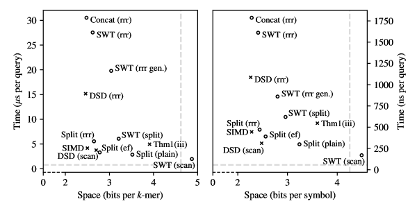
The test results for the metagenome data set can be seen in Figure 2; the results for the E. Coli data set are similar. See appendix A for the data belonging to Figure 2, and appendix B for the results of the data structures omitted from this figure. The fastest structure is SWT (scan), but it is large and is outperformed by the benchmark solution on both parameters. Our unoptimized reduction Thm1(iii) uses more space than the remaining structures of [2, 3] while remaining within a factor two in query time of most of them. Our fastest structure, DSD (scan), is competitive with both Split (ef) and Split (rrr). Our most compact structure DSD (rrr) matches the space of the previous smallest structure, Concat (ef), while supporting queries twice as fast. Our SIMD-enhanced structure uses less than one percent more space than Concat (ef) while supporting queries four to seven times faster. It is also competitive with the fast and compact structures Split (ef) and Split (rrr). We note that the entropies for the distributions of sets in the Metagenome and E. Coli data sets are respectively and bits (as seen in [2]), and that reduction from bits (Split (rrr), Metagenome) to bits (SIMD, Metagenome) reduces the distance to the entropy from approximately to , while simultaneously supporting queries faster.
References
- [1] Karl R. Abrahamson. Generalized string matching. SIAM J. Comput., 16(6):1039–1051, 1987. doi:10.1137/0216067.
- [2] Jarno N. Alanko, Elena Biagi, Simon J. Puglisi, and Jaakko Vuohtoniemi. Subset wavelet trees. In Proc. 21st SEA, pages 4:1–4:14, 2023. doi:10.4230/LIPIcs.SEA.2023.4.
- [3] Jarno N. Alanko, Simon J. Puglisi, and Jaakko Vuohtoniemi. Small searchable -spectra via subset rank queries on the spectral burrows-wheeler transform. In Proc. ACDA, 2023, pages 225–236, 2023. doi:10.1137/1.9781611977714.20.
- [4] Mai Alzamel, Lorraine A. K. Ayad, Giulia Bernardini, Roberto Grossi, Costas S. Iliopoulos, Nadia Pisanti, Solon P. Pissis, and Giovanna Rosone. Comparing degenerate strings. Fundam. Informaticae, 175(1-4):41–58, 2020. doi:10.3233/FI-2020-1947.
- [5] Jérémy Barbay, Francisco Claude, Travis Gagie, Gonzalo Navarro, and Yakov Nekrich. Efficient fully-compressed sequence representations. Algorithmica, 69(1):232–268, 2014. doi:10.1007/S00453-012-9726-3.
- [6] Jérémy Barbay, Meng He, J. Ian Munro, and Srinivasa Rao Satti. Succinct indexes for strings, binary relations and multilabeled trees. ACM Trans. Algorithms, 7(4):52:1–52:27, 2011. doi:10.1145/2000807.2000820.
- [7] Djamal Belazzougui, Patrick Hagge Cording, Simon J. Puglisi, and Yasuo Tabei. Access, rank, and select in grammar-compressed strings. In Proc. 23rd ESA, pages 142–154, 2015. doi:10.1007/978-3-662-48350-3\_13.
- [8] Djamal Belazzougui and Gonzalo Navarro. Optimal lower and upper bounds for representing sequences. ACM Trans. Algorithms, 11(4):31:1–31:21, 2015. doi:10.1145/2629339.
- [9] David R. Clark and J. Ian Munro. Efficient suffix trees on secondary storage (extended abstract). In Proc. 7th SODA, pages 383–391, 1996. URL: http://dl.acm.org/citation.cfm?id=313852.314087.
- [10] Maxime Crochemore, Costas S. Iliopoulos, Tomasz Kociumaka, Jakub Radoszewski, Wojciech Rytter, and Tomasz Walen. Covering problems for partial words and for indeterminate strings. Theor. Comput. Sci., 698:25–39, 2017. doi:10.1016/J.TCS.2017.05.026.
- [11] Paolo Ferragina, Giovanni Manzini, Veli Mäkinen, and Gonzalo Navarro. Compressed representations of sequences and full-text indexes. ACM Trans. Algorithms, 3(2):20, 2007. doi:10.1145/1240233.1240243.
- [12] Travis Gagie. Rank and select operations on sequences. In Encyclopedia of Algorithms, pages 1776–1780. 2016. doi:10.1007/978-1-4939-2864-4\_638.
- [13] Simon Gog, Timo Beller, Alistair Moffat, and Matthias Petri. From theory to practice: Plug and play with succinct data structures. In Proc. 13th SEA, pages 326–337, 2014.
- [14] Alexander Golynski, J. Ian Munro, and S. Srinivasa Rao. Rank/select operations on large alphabets: a tool for text indexing. In Proc. 15th SODA, pages 368–373, 2006. URL: http://dl.acm.org/citation.cfm?id=1109557.1109599.
- [15] Alexander Golynski, Alessio Orlandi, Rajeev Raman, and S. Srinivasa Rao. Optimal indexes for sparse bit vectors. Algorithmica, 69(4):906–924, 2014. doi:10.1007/S00453-013-9767-2.
- [16] Roberto Grossi, Ankur Gupta, and Jeffrey Scott Vitter. High-order entropy-compressed text indexes. In Proc. 14th SODA, pages 841–850, 2003.
- [17] Roberto Grossi, Rajeev Raman, Srinivasa Rao Satti, and Rossano Venturini. Dynamic compressed strings with random access. In Proc. 40th ICALP, pages 504–515, 2013. doi:10.1007/978-3-642-39206-1\_43.
- [18] Meng He and J. Ian Munro. Succinct representations of dynamic strings. In Proc. 17th SPIRE, pages 334–346, 2010. doi:10.1007/978-3-642-16321-0\_35.
- [19] Costas S. Iliopoulos, Laurent Mouchard, and Mohammad Sohel Rahman. A new approach to pattern matching in degenerate DNA/RNA sequences and distributed pattern matching. Math. Comput. Sci., 1(4):557–569, 2008. doi:10.1007/S11786-007-0029-Z.
- [20] Guy Jacobson. Space-efficient static trees and graphs. In Proc. FOCS, pages 549–554, 1989. doi:10.1109/SFCS.1989.63533.
- [21] Ian B Jeffery, Anubhav Das, Eileen O’Herlihy, Simone Coughlan, Katryna Cisek, Michael Moore, Fintan Bradley, Tom Carty, Meenakshi Pradhan, Chinmay Dwibedi, et al. Differences in fecal microbiomes and metabolomes of people with vs without irritable bowel syndrome and bile acid malabsorption. Gastroenterology, 158(4):1016–1028, 2020.
- [22] Danyang Ma, Simon J Puglisi, Rajeev Raman, and Bella Zhukova. On elias-fano for rank queries in fm-indexes. In Proc. DCC, 2021, pages 223–232, 2021.
- [23] Veli Mäkinen and Gonzalo Navarro. Rank and select revisited and extended. Theor. Comput. Sci., 387(3):332–347, 2007. doi:10.1016/J.TCS.2007.07.013.
- [24] Gonzalo Navarro and Yakov Nekrich. Optimal dynamic sequence representations. SIAM J. Comput., 43(5):1781–1806, 2014. doi:10.1137/130908245.
- [25] Gonzalo Navarro and Kunihiko Sadakane. Fully functional static and dynamic succinct trees. ACM Trans. Algorithms, 10(3):16:1–16:39, 2014. doi:10.1145/2601073.
- [26] Daisuke Okanohara and Kunihiko Sadakane. Practical Entropy-Compressed Rank/Select Dictionary. In Proc. 9th ALENEX, 2007. doi:10.1137/1.9781611972870.6.
- [27] Alberto Ordóñez Pereira, Gonzalo Navarro, and Nieves R. Brisaboa. Grammar compressed sequences with rank/select support. J. Discrete Algorithms, 43:54–71, 2017. doi:10.1016/J.JDA.2016.10.001.
- [28] Rajeev Raman, Venkatesh Raman, and Srinivasa Rao Satti. Succinct indexable dictionaries with applications to encoding k-ary trees, prefix sums and multisets. ACM Trans. Algorithms, 3(4):43, 2007. doi:10.1145/1290672.1290680.
Appendix A Additional Data
| -mer Queries | Subset Rank Queries | |||||||
| E. Coli | Metagenome | E. Coli | Metagenome | |||||
| Data structure | Query | Space | Query | Space | Query | Space | Query | Space |
| (s) | (bpk) | (s) | (bpk) | (ns) | (bps) | (ns) | (bps) | |
| Matrix | 0.63 | 4.29 | 0.77 | 4.62 | 38.75 | 4.26 | 56.98 | 4.25 |
| DSD (scan) | 3.00 | 2.61 | 3.75 | 2.70 | 210.23 | 2.57 | 311.33 | 2.48 |
| Thm1(iii) | 3.87 | 3.68 | 4.95 | 3.91 | 435.28 | 3.64 | 546.89 | 3.60 |
| DSD (rrr) | 13.21 | 2.38 | 15.17 | 2.46 | 850.99 | 2.34 | 1086.11 | 2.26 |
| SIMD | 3.31 | 2.42 | 4.16 | 2.50 | 320.53 | 2.37 | 444.94 | 2.28 |
| SWT (scan) | 1.63 | 4.53 | 1.96 | 4.87 | 129.44 | 4.49 | 170.44 | 4.49 |
| SWT (split) | 4.93 | 3.17 | 6.06 | 3.21 | 436.69 | 3.13 | 620.47 | 2.96 |
| SWT (rrr gen.) | 18.97 | 2.84 | 19.79 | 3.04 | 789.12 | 2.81 | 860.4 | 2.80 |
| SWT (rrr) | 25.33 | 2.48 | 27.55 | 2.62 | 1384.0 | 2.45 | 1610.73 | 2.41 |
| Split (plain) | 2.28 | 3.30 | 2.84 | 3.52 | 235.22 | 3.27 | 298.87 | 3.24 |
| Split (ef) | 2.71 | 2.69 | 3.30 | 2.78 | 317.71 | 2.65 | 390.65 | 2.56 |
| Split (rrr) | 4.70 | 2.54 | 5.54 | 2.65 | 393.14 | 2.51 | 471.30 | 2.44 |
| Concat(ef) | 26.25 | 2.38 | 30.53 | 2.48 | 1372.2 | 2.35 | 1786.65 | 2.28 |
Appendix B Results for all Data Structures
This section elaborates on the data structures that were omitted from Sections 5.2 and 6. From [3], we omitted the structure Concat (plain), which is the structure Concat (ef) explained in Section 5.2 parameterized with standard SDSL bitvcectors instead. We also omitted Matrix (ef) and Matrix (rrr), which is the benchmark solution parameterized with different types of bitvectors.
Furthermore, this section includes more parameterizations of our SIMD enhnaced data structure. We elaborate on the SIMD structure from Section 5.2. DSD (SIMD (i)) (which we refer to as SIMD (i) for simplicity) is the DSD parameterized with the SIMD (i) structure, which supports rank queries on strings over the alphabet . As described in Section 5.2, the main idea is to divide the string into blocks, precompute the answer to rank queries up to the start of each block, and compute partial rank queries internally in blocks as needed using SIMD. The width of the block is determined by the parameter ; there are characters stored per block (recall that the width of the SIMD registers we used was bits). The blocks are stored as follows. Each character in consists of two bits. We separate the string represented by the block into two bitstrings; one consisting of the low bits, and one of the high bits. To compute partial rank queries, we use the operation vpternlogq, which given three vectors and an -bit integer value evaluates any three-variable boolean function bit-wise for the three vectors (the -bit integer describes the result column of the three-variable truth table, which has eight rows). The operation also accepts an additional integer, used to mask out results if they are not needed for the computation. To answer rank queries, we traverse the low and high bitstrings, using vpternlogq to find occurrences of the queried character and the mask to filter out results occurring after the queried index. The version of the SIMD data structure in Sections 5.2 and 6 is SIMD (8).
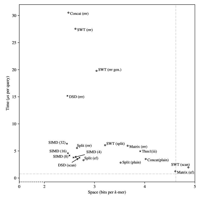
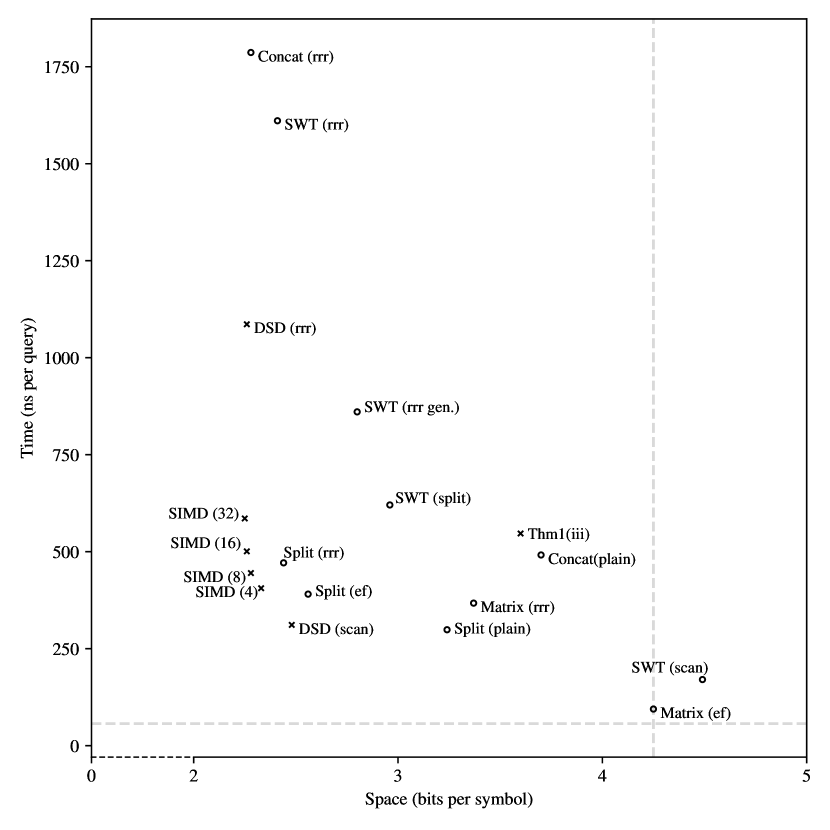
The results for all the structures on the metagenome data set can be seen in Figure 3 (-mer search test) and Figure 4 (rank query benchmark). All the data, for all structures, both data sets, and both tests, can be seen in Table 2.
| -mer Queries | Subset Rank Queries | |||||||
| E. Coli | Metagenome | E. Coli | Metagenome | |||||
| Data structure | Query | Space | Query | Space | Query | Space | Query | Space |
| (s) | (bpk) | (s) | (bpk) | (ns) | (bps) | (ns) | (bps) | |
| Matrix | 0.63 | 4.29 | 0.77 | 4.62 | 38.75 | 4.26 | 56.98 | 4.25 |
| Matrix (ef) | 0.92 | 4.07 | 1.24 | 4.61 | 73.9 | 4.04 | 94.4 | 4.25 |
| Matrix (rrr) | 5.28 | 3.38 | 5.96 | 3.66 | 301.7 | 3.34 | 367.45 | 3.37 |
| DSD (scan) | 3.0 | 2.61 | 3.75 | 2.7 | 210.23 | 2.57 | 311.33 | 2.48 |
| Thm1(iii) | 3.87 | 3.68 | 4.95 | 3.91 | 435.28 | 3.64 | 546.89 | 3.6 |
| DSD (rrr) | 13.21 | 2.38 | 15.17 | 2.46 | 850.99 | 2.34 | 1086.11 | 2.26 |
| SIMD (4) | 2.98 | 2.49 | 3.79 | 2.58 | 289.54 | 2.42 | 405.88 | 2.33 |
| SIMD (8) | 3.31 | 2.42 | 4.16 | 2.5 | 320.53 | 2.37 | 444.94 | 2.28 |
| SIMD (16) | 3.67 | 2.39 | 4.58 | 2.47 | 371.87 | 2.35 | 500.97 | 2.26 |
| SIMD (32) | 5.35 | 2.37 | 6.34 | 2.45 | 447.28 | 2.34 | 585.65 | 2.25 |
| SWT (scan) | 1.63 | 4.53 | 1.96 | 4.87 | 129.44 | 4.49 | 170.44 | 4.49 |
| SWT (split) | 4.93 | 3.17 | 6.06 | 3.21 | 436.69 | 3.13 | 620.47 | 2.96 |
| SWT (rrr gen.) | 18.97 | 2.84 | 19.79 | 3.04 | 789.12 | 2.81 | 860.4 | 2.8 |
| SWT (rrr) | 25.33 | 2.48 | 27.55 | 2.62 | 1384.0 | 2.45 | 1610.73 | 2.41 |
| Concat(plain) | 2.53 | 3.74 | 3.51 | 4.02 | 375.44 | 3.71 | 491.55 | 3.7 |
| Concat(ef) | 26.25 | 2.38 | 30.53 | 2.48 | 1372.2 | 2.35 | 1786.65 | 2.28 |
| Split (plain) | 2.28 | 3.3 | 2.84 | 3.52 | 235.22 | 3.27 | 298.87 | 3.24 |
| Split (ef) | 2.71 | 2.69 | 3.3 | 2.78 | 317.71 | 2.65 | 390.65 | 2.56 |
| Split (rrr) | 4.7 | 2.54 | 5.54 | 2.65 | 393.14 | 2.51 | 471.3 | 2.44 |