Kinetic description and macroscopic limit of swarming dynamics with continuous leader-follower transitions

Abstract

In this paper, we derive a kinetic description of swarming particle dynamics in an interacting multi-agent system featuring emerging leaders and followers. Agents are classically characterized by their position and velocity plus a continuous parameter quantifying their degree of leadership. The microscopic processes ruling the change of velocity and degree of leadership are independent, non–conservative and non–local in the physical space, so as to account for long–range interactions. Out of the kinetic description, we obtain then a macroscopic model under a hydrodynamic limit reminiscent of that used to tackle the hydrodynamics of weakly dissipative granular gases, thus relying in particular on a regime of small non–conservative and short–range interactions. Numerical simulations in one- and two-dimensional domains show that the limiting macroscopic model is consistent with the original particle dynamics and furthermore can reproduce classical emerging patterns typically observed in swarms.

Keywords: swarm dynamics, transient leadership, Povzner-Boltzmann equation, hydrodynamic limit, non-conservative interactions

Mathematics Subject Classification: 35Q20, 35Q70, 92D50.

1 Introduction

In this paper, we are concerned with kinetic and hydrodynamic modelling of swarming dynamics in self-organising multi-agent systems with group behaviour and transient leadership, biologically inspired by flocks of birds.

A first introduction to the collective motion of groups of animals can be found in [58, 61]. Concerning flocking birds, many of the underlying mechanisms have been unveiled by several experimental studies, mostly from a physical perspective, based on tracking and analysing the trajectories of flying birds [8, 9, 10, 11, 26, 27, 29, 45, 56] and by other experiments made within similar goals [44, 50, 54, 57]. These investigations have put in evidence that birds interact within a certain perception range, tend to align with the flight direction of neighbours and rely on a variable-in-time interaction network, as each bird changes its neighbours continuously while moving [29]. In particular, the two already cited papers [9, 44] focus on coherent changes in the direction of motion of the group as a whole. They find that collective turns have a localised spatial origin: they are triggered by few members of the flock, that act locally as leaders, and happen spontaneously, i.e. without external stimuli (such as e.g., a predator attack). Another important biological mechanism observed in several animal groups, including flocks of birds, is the switch of leaders [18, 30, 49]: since all group members may be leaders temporarily, leaders change continuously, with former leaders becoming followers and then again leaders after a while. The leader-follower transition is often difficult to understand, because in some flocks of birds, such as e.g., pigeons, it is associated with a continuous degree of leadership, which determines a hierarchy of leaders based e.g., on the ability of birds to act as turning initiators [41, 52].

As far as the mathematical modelling and numerical simulation of swarming dynamics are concerned, we mention first the three seminal papers [31, 37, 60], which have shown how simple algorithms based on elementary interaction rules can generate apparently complex self-organised collective movements. Following these works, many other microscopic models including leaders have been proposed, see e.g., [4, 15, 16, 48], sometimes inspired by analogies with fundamental physical principles such as e.g., the inertial spin models [12, 28, 47]. Microscopic models allow for exhaustive simulations when the total number of agents, say $N$, is large enough, for then statistical average quantities may be regarded as consistent descriptors of the aggregate behaviour. Nevertheless, one experiences the well-known drawback that the computational cost of a microscopic simulation scales typically as $\mathcal{O}(N)$ or $\mathcal{O}(N^{2})$, depending on the specific microscopic model, whereas the cost of a macroscopic simulation would be independent of $N$. Moreover, microscopic models are hardly amenable to analytical investigations of the emerging aggregate behaviour of the particle system.

For these reasons, several mesoscopic and macroscopic models have also been proposed and studied [14, 17, 19, 20, 21, 22, 23, 24, 25, 38, 40]. Among them, we focus in particular on kinetic models, i.e. mesoscopic models which can be formally derived from interacting particle dynamics as evolution equations of the time-dependent probability distribution of the microscopic state of the interacting particles. Particle dynamics may be stated in terms of either ordinary or stochastic differential equations. Kinetic equations are then derived either as mean-field limits of the particle dynamics for $N\to\infty$, see e.g., [1], or as statistical descriptions of the stochastic microscopic interaction processes [51].

In this paper, we adopt the point of view of the classical kinetic theory, having its roots in gas dynamics and nowadays fruitfully revisited and applied to the mathematical description of a great variety of interaction phenomena, cf. [51] and references therein. The leading idea is that agents are identified to a microscopic state, which changes in consequence of interactions and is described statistically by means of a probability distribution defined on an appropriate continuous phase space. Typically, interactions are assumed to be binary processes, i.e. each of them involves two agents at a time. Interactions involving simultaneously more than two particles are neglected as higher order effects. Kinetic models for collective dynamics incorporating leaders and followers have been introduced in [2, 4, 5, 7, 13]. In this case, agents are described by their position, velocity and a discrete label denoting either leadership or followership, which may change in time. Kinetic equations with label switching have been formally analysed in [46] and applied to the modelling of collective dynamics in the presence of switching leaders in [6]. Kinetic models also allow one to derive macroscopic models, which inherit naturally the details of the microscopic particle dynamics. This is typically carried out by introducing as average macroscopic quantities the statistical moments of the probability distribution of the microscopic state. Their evolution equations are then obtained either from a hydrodynamic limit or through asymptotic expansions (Hilbert, Chapman-Enskog). These procedures lead to closed systems of evolution equations for the average macroscopic quantities in specific regimes of the microscopic parameters [1, 24, 40].

In the present work, our starting point is the microscopic model proposed in [34], which describes the dynamics of turning and flocking birds, like starlings or jackdaws. The model is based on the well-established attraction-alignment-repulsion paradigm [32, 38, 58, 61] and is specifically conceived to reproduce spontaneous (i.e., not caused by external stimuli) sudden self-organised changes of direction of motion. Moreover, the model assumes that each bird is a potential turn initiator, meaning that a sort of temporary leadership emerges in a group of indistinguishable birds. Retaining the fundamental ingredients of this model, we focus on an analytical description based on kinetic equations and their macroscopic limits. More specifically, we define a multi-agent system whose agents are characterised by space position and velocity plus a continuous parameter quantifying their degree of leadership. We formulate discrete-in-time stochastic particle dynamics inspired by a simplified version of the microscopic model introduced in [34] and featuring non-local binary interactions, so as to take into account that agents may affect each other possibly within an interaction range. The microscopic processes ruling the change of velocity and degree of leadership are independent and both non-conservative, except for the mass. Therefore, to derive formally kinetic and macroscopic descriptions implementing such microscopic dynamics we resort to a Povzner-Boltzmann-type equation [55] with corrections to the collisional operator suitable to take into account the non-conservativeness of the microscopic interactions when passing to the hydrodynamic limit. For this, we adapt the technique proposed in [40], where the authors perform the hydrodynamic limit of the Povzner-Boltzmann equation for a system of agents having the velocity as a unique microscopic state. There, the binary interaction rules are non-local and non-conservative as well and, in particular, they are given by the classical conservative hard-spheres collisions plus a dissipative contribution. The key idea is to consider the regime in which the non-conservative contribution is small, in such a way that the leading part of the interaction rules is given by the classical velocity- and energy-preserving hard-spheres mechanism, while the dissipative part is of higher order. This allows the authors to approximate the non-local Maxwellian relative to the leading order terms of the interaction rules with the classical local Maxwellian. In our case, the main difficulty is that this idea has to be evolved to treat multiple microscopic states with different non-mechanical non-conservativeness.

The plan of the paper, after this Introduction, is the following. In Section 2 we revise and summarise the main aspects of the microscopic models presented in [34]. Then in Section 3 we introduce our discrete-in-time stochastic particle model implementing the interaction dynamics discussed above and derive formally the corresponding Povzner-Boltzmann kinetic equation. In Section 4 we derive our macroscopic model of swarming dynamics with transient leadership and continuous leader-follower transitions as a hydrodynamic limit of the Povzner-Boltzmann equation. Next, in Section 5 we discuss some numerical tests, which we use to elucidate the correspondence between the original stochastic particle model and the resulting macroscopic description (in one space dimension) as well as to show that the macroscopic model reproduces successfully (in two space dimensions) some classical swarming patterns, such as splitting and merging of the flock and rings/mills. Finally, in Section 6 we draw some conclusions and briefly sketch possible research perspectives.

2 Microscopic outlook

We consider a group of $N>1$ agents represented as point masses in $\mathbb{R}^{d}$, $d\geq 1$. We assume that they are labelled univocally by an index $k=1,\,\dots,\,N$ and we denote by $X_{k}(t),\,V_{k}(t)\in\mathbb{R}^{d}$ the position and velocity of the $k$-th agent at time $t$, respectively. We also distinguish agents in terms of leaders and followers. This distinction is not permanent, since agents can change status in time. Leaders do not have any particular knowledge or experience compared to other agents, their role is just to initiate turns. To this aim, they try to get far from the group – the flock from now on – at least until they get back to the status of followers. Roughly speaking, the idea is that any agent can attempt to steer the flock by initiating a turn, but the attempt has a limited duration and if turning is not triggered within a reasonable time the attempt is aborted. Here we consider the leader/follower status as a spectrum, meaning that agents exhibit a possibly non-binary behavior between the statuses of leader and follower. We denote by $\Lambda_{k}=\Lambda_{k}(t)\in[0,\,1]$ the degree of leadership of agent $k$ at time $t$, being $\Lambda_{k}=0$ the pure follower behavior and $\Lambda_{k}=1$ the pure leader behavior.

Concerning interactions, we assume that agents are influenced by flock mates within a certain fixed distance $R>0$ only (metric interaction). It is worth noting that in the microscopic model introduced in [34], unlike the one studied here, interactions are topological [11] and the distinction between leaders and followers is sharp, in the sense that at any given time an agent is either a leader or a follower. We refer to [6] for a kinetic model which retains these features.

In the same spirit as in [34], we consider the following second order dynamics:

$$\ddot{X}_{k}=\mu\mathcal{A}_{k}(\mathbf{X},\mathbf{V},\Lambda_{k}),\qquad k=1,\,\dots,\,N,$$ (1)

where $\mathbf{X}:=(X_{1},\,\dots,\,X_{N})$, $\mathbf{V}:=(V_{1},\,\dots,\,V_{N})$, $\mu>0$ is a parameter fixing the time scale and the acceleration $\mathcal{A}_{k}$ is given by the sum of three terms accounting respectively for repulsion, alignment, and attraction among the agents:

$$\mathcal{A}_{k}(\mathbf{X},\mathbf{V},\Lambda_{k}):=\sum_{X_{h}\in B_{R}(X_{k})}\left[\alpha\frac{X_{k}-X_{h}}{\left\lvert X_{k}-X_{h}\right\rvert^{2}}+(1-\Lambda_{k})\Bigl{(}\beta(V_{h}-V_{k})+\gamma(X_{h}-X_{k})\Bigr{)}\right].$$ (2)

Here, $B_{R}(X_{k})\subset\mathbb{R}^{d}$ is the ball of radius $R>0$ centered in $X_{k}$ (metric neighborhood) and $\alpha,\,\beta,\,\gamma>0$ are parameters calibrating the mutual strength of the three types of interaction. We notice that, unlike other approaches in the reference literature, here we choose for simplicity to consider all types of interaction simultaneously active within the interaction neighborhood $B_{R}(X_{k})$. We will see in the numerical tests that this simplification does not preclude the possibility to reproduce well-known self-organized patterns of the flock. We also point out that, while repulsion is common to both leaders and followers, alignment and attraction characterize preferentially the interaction dynamics of the followers, cf. the coefficient $1-\Lambda_{k}$ in front of the last two terms in (2).

While the repulsion-alignment-attraction paradigm is nowadays standard and well accepted in the modeling of flock dynamics, the evolution of $\Lambda_{k}$, driving the leader-follower transition, is much less investigated. In particular, we do not have any biological clue for this term. Therefore, we appeal to the general idea that the $\Lambda_{k}$’s are independent and identically distributed random variables supported in $[0,\,1]$ and sampled at random instants. This way, agents continuously switch their (non-binary) status between leader, follower and intermediate nuances.

3 Kinetic approach

As anticipated in the Introduction, the goal of this paper is to derive a hydrodynamic model of flock dynamics inspired by the ideas outlined in Section 2 and incorporating, in particular, the leader-follower transitions. The novelty with respect to the mainstream in the literature is that we do not rely on separate descriptions of leaders and followers with possible mass transfers between the two populations. Instead, we give a unique fluid dynamical representation of the flock, which embeds consistently the gross evolution of the degree of leadership of the agents.

To pursue this goal, we take advantage of the methods of statistical mechanics in general and of the kinetic theory in particular, which provide powerful mathematical tools to upscale consistently simple particle dynamics to complex aggregate macroscopic trends.

3.1 Stochastic particle model

We assume that the flock can be regarded as a large ensemble of indistinguishable agents. A generic representative agent is described at time $t>0$ by the position in space $X_{t}\in\mathbb{R}^{d}$, the velocity $V_{t}\in\mathbb{R}^{d}$ and degree of leadership $\Lambda_{t}\in[0,\,1]$. To adopt a statistical point of view, we regard $X_{t}$, $V_{t}$, $\Lambda_{t}$ as random variables with joint distribution

$$f=f(x,v,\lambda,t):\mathbb{R}^{d}\times\mathbb{R}^{d}\times[0,\,1]\times[0,\,+\infty)\to\mathbb{R}_{+}$$ (3)

such that $f(x,v,\lambda,t)\,dx\,dv\,d\lambda$ is the probability that at time $t$ a generic agent of the flock has a position in the infinitesimal volume element $dx$ centered in $x$, a velocity in the infinitesimal volume element $dv$ centered in $v$ and a degree of leadership comprised between $\lambda$ and $\lambda+d\lambda$.

The evolution of the stochastic processes $\{X_{t},\,t\geq 0\}$, $\{V_{t},\,t\geq 0\}$, $\{\Lambda_{t},\,t\geq 0\}$ is motivated by the considerations expressed in Section 2. In particular, referring to a discrete time setting for simplicity but with the idea to pass subsequently to the continuous time limit, we invoke the usual kinematic relationship between $X_{t}$ and $V_{t}$ to state that at the new time $t+\Delta{t}$, with $\Delta{t}>0$, a generic agent of the flock changes position because of a free drift:

$$X_{t+\Delta{t}}=X_{t}+V_{t}\Delta{t}.$$ (4)

On the other hand, the new velocity of the agent is determined by an interaction process inspired by (1)-(2) with another agent sampled randomly in the flock, as prescribed by the scheme of binary interactions of the classical kinetic theory. If $(X_{t}^{\ast},\,V_{t}^{\ast},\,\Lambda_{t}^{\ast})$ is the microscopic state of the other agent then we set

$$V_{t+\Delta{t}}=V_{t}+\Theta\mathcal{A}(X_{t},X_{t}^{\ast},V_{t},V_{t}^{\ast},\Lambda_{t},\Lambda_{t}^{\ast}),$$ (5)

where

$$\mathcal{A}(X_{t},X_{t}^{\ast},V_{t},V_{t}^{\ast},\Lambda_{t},\Lambda_{t}^{\ast})=\alpha\dfrac{X_{t}-X_{t}^{\ast}}{\left\lvert X_{t}-X_{t}^{\ast}\right\rvert^{2}}+(1-\Lambda_{t})\Bigl{(}\beta(V_{t}^{\ast}-V_{t})+\gamma(X_{t}^{\ast}-X_{t})\Bigr{)},$$ (6)

while $\Theta\in\{0,\,1\}$ is a random variable discriminating whether, in the time step $\Delta{t}$, an interaction between the two sampled agents may actually take place. Specifically, we set

$$\Theta\sim\operatorname{Bernoulli}(\mu B(\left\lvert X_{t}^{\ast}-X_{t}\right\rvert)\Delta{t}),$$ (7)

i.e. $\mu B(\left\lvert X_{t}^{\ast}-X_{t}\right\rvert)\Delta{t}$ is the probability that an interaction between the two sampled agents takes place in the time interval $[t,\,t+\Delta{t}]$. In more detail, $\mu>0$ is the rate of velocity change while $B(\left\lvert X_{t}^{\ast}-X_{t}\right\rvert)\geq 0$ is the collision kernel, which fixes the rate at which agents at a given distance $\left\lvert X_{t}^{\ast}-X_{t}\right\rvert$ may interact. We assume that $B=B(r)$, $r\in\mathbb{R}_{+}$, is a non-negative bounded function supported in the interval $[0,\,R]\subset\mathbb{R}_{+}$ for a given radius $R\in(0,\,+\infty)$. This reproduces the idea of metric interactions within the interaction range $R$. Consequently, the mapping $\mathbb{R}^{d}\ni x\mapsto B(\left\lvert x\right\rvert)$ is radially symmetric and supported in the ball $\mathscr{B}_{R}(0)\subset\mathbb{R}^{d}$ of radius $R$ and centred at the origin.

Finally, we postulate the following update process of the degree of leadership:

$$\Lambda_{t+\Delta t}=\Lambda_{t}+\Sigma(1-2\Lambda_{t}),$$ (8)

where $\Sigma\in\{0,\,1\}$ is a new random variable, independent of $\Theta$, distributed as

$$\Sigma\sim\operatorname{Bernoulli}(\eta B(\left\lvert X_{t}^{\ast}-X_{t}\right\rvert)\Delta{t})$$ (9)

with $\eta>0$ the rate of degree change. Notice that (9) implies that a change in the degree of leadership of one agent is stimulated by the presence of the other agent in the interaction neighborhood. Nevertheless, according to (8) the new degree of leadership of either agent does not depend on the current degree of leadership of the other agent. In other words, we assume that agents become leaders or followers spontaneously and not e.g., by imitation or contrast. We also remark that (8) is such that

$$\Lambda_{t+\Delta t}=\begin{cases}\Lambda_{t}&\text{if }\Sigma=0\\ 1-\Lambda_{t}&\text{if }\Sigma=1,\end{cases}$$

meaning that any agent undergoes continuously a switch of its degree of leadership between the initial value $\Lambda_{0}$ and the symmetric one $1-\Lambda_{0}$ with respect to the mid-value $\frac{1}{2}$.

For the sake of completeness, we point out that (7), (9) require

$$\Delta{t}\leq\frac{1}{\max{\{\mu,\,\eta\}}\sup\limits_{x\in\mathscr{B}_{R}(0)}B(\left\lvert x\right\rvert)}$$

as a sufficient consistency condition. However, such a constraint is not a limitation in the continuous time limit $\Delta{t}\to 0^{+}$.

3.2 Boltzmann-type description

A Boltzmann-type description of the flocking particle dynamics discussed in Section 3.1 consists in a collisional kinetic equation for the distribution function (3), which, being regarded as a probability distribution, is assumed to be non-negative and such that

$$\int_{0}^{1}\int_{\mathbb{R}^{d}}\int_{\mathbb{R}^{d}}f(x,v,\lambda,t)\,dx\,dv\,d\lambda=1,\qquad\forall\,t>0.$$

Averaging the discrete time stochastic processes (4), (5), (8) and passing to the limit $\Delta{t}\to 0^{+}$, by standard arguments (cf. e.g., [51]) we obtain the following Boltzmann-type kinetic equation for $f$:

$$\partial_{t}f+v\cdot\nabla_{x}f=\mu Q^{v}(f,f)+\eta Q^{\lambda}(f,f),$$ (10)

where $Q^{v}$ and $Q^{\lambda}$ are the collisional operators implementing, at the kinetic level, the independent particle processes (5), (8), respectively. More specifically, these two operators are univocally defined by the following weak formulations:

$$\begin{aligned} \left\langle Q^{v}(f,f),\,\varphi\right\rangle&:=\int_{0}^{1}\int_{\mathbb{R}^{d}}Q^{v}(f,f)(x,v,\lambda,t)\varphi(v,\lambda)\,dv\,d\lambda\\ &=\int_{[0,\,1]^{2}}\int_{\mathbb{R}^{3d}}B(\left\lvert x_{\ast}-x\right\rvert)\big{(}\varphi(v^{\prime},\lambda)-\varphi(v,\lambda)\big{)}ff_{\ast}\,dx_{\ast}\,dv\,dv_{\ast}\,d\lambda\,d\lambda_{\ast},\end{aligned}$$ (11)

where, here and henceforth, $f$ and $f_{\ast}$ are shorthand for $f(x,v,\lambda,t)$ and $f(x_{\ast},v_{\ast},\lambda_{\ast},t)$, respectively, and

$$\begin{aligned} \left\langle Q^{\lambda}(f,f),\,\varphi\right\rangle&:=\int_{0}^{1}\int_{\mathbb{R}^{d}}Q^{\lambda}(f,f)(x,v,\lambda,t)\varphi(v,\lambda)\,dv\,d\lambda\\ &=\int_{[0,\,1]^{2}}\int_{\mathbb{R}^{3d}}B(\left\lvert x_{\ast}-x\right\rvert)\big{(}\varphi(v,\lambda^{\prime})-\varphi(v,\lambda)\big{)}ff_{\ast}\,dx_{\ast}\,dv\,dv_{\ast}\,d\lambda\,d\lambda_{\ast},\end{aligned}$$ (12)

where $\varphi:\mathbb{R}^{d}\times[0,\,1]\to\mathbb{R}$, $\varphi=\varphi(v,\lambda)$, is an arbitrary test function representing any observable quantity whereas

$$v^{\prime}=v+\alpha\frac{x-x_{\ast}}{\left\lvert x-x_{\ast}\right\rvert^{2}}+(1-\lambda)\bigl{(}\beta(v_{\ast}-v)+\gamma(x_{\ast}-x)\bigr{)}$$ (13)

is the post-collisional velocity determined by an interaction of the form (5)-(6) and

$$\lambda^{\prime}=1-\lambda$$ (14)

is the post-collisional degree of leadership produced by the microscopic rule (8). The other agent participating in the binary interaction modifies symmetrically its velocity and degree of leadership according to the rules

$$v_{\ast}^{\prime} =v_{\ast}+\alpha\frac{x_{\ast}-x}{\left\lvert x_{\ast}-x\right\rvert^{2}}+(1-\lambda_{\ast})\bigl{(}\beta(v-v_{\ast})+\gamma(x-x_{\ast})\bigr{)},$$ (15)

$$\lambda_{\ast}^{\prime} =1-\lambda_{\ast}.$$ (16)

In (11)-(12) the kernel $B$ -classically called the Povzner kernel- takes into account the fact that the particle processes are not localized in the physical space. Hence, the Boltzmann-type kinetic equation (10) may be also called Boltzmann-Povzner equation.

Remark 3.1.

In each binary interaction neither the mean velocity nor the mean degree of leadership is conserved in general. Indeed,

$$v^{\prime}+v_{\ast}^{\prime}-(v+v_{\ast})=(\lambda_{\ast}-\lambda)\bigl{(}\beta(v_{\ast}-v)+\gamma(x_{\ast}-x)\bigr{)}$$

$$\lambda^{\prime}+\lambda_{\ast}^{\prime}-(\lambda+\lambda_{\ast})=2\bigl{(}1-(\lambda+\lambda_{\ast})\bigr{)}.$$

Multiplying (10) by $\varphi$ and integrating w.r.t. $v$, $\lambda$ we obtain the weak form of the Boltzmann-type kinetic equation, which reads

$$\partial_{t}\int_{0}^{1}\int_{\mathbb{R}^{d}}\varphi(v,\lambda)f(x,v,\lambda,t)\,dv\,d\lambda+\operatorname{div}_{x}\int_{0}^{1}\int_{\mathbb{R}^{d}}\varphi(v,\lambda)vf(x,v,\lambda,t)\,dv\,d\lambda\\ =\mu\left\langle Q^{v}(f,f),\,\varphi\right\rangle+\eta\left\langle Q^{\lambda}(f,f),\,\varphi\right\rangle.$$ (17)

For completeness, we point out that the collisional operators $Q^{v}(f,f)$, $Q^{\lambda}(f,f)$ may be written explicitly also in strong form. However, since for the sequel the latter is less useful than (11), (12), we confine it to Appendix A, cf. (52), (53).

3.3 Approximation in the regime of small non-conservative interactions

In classical kinetic theory, the derivation of macroscopic equations via the hydrodynamic limit relies heavily on the concept of collisional invariants, which are observable quantities conserved, on average, by the particle interactions. Collisional invariants are usually sought in the form of powers of the variables characterizing the microscopic state of the particles, which are at the basis of the computation of the statistical moments of the kinetic distribution function.

As pointed out in Remark 3.1, the interaction rules (13)-(15) and (14)-(16) are pointwise non-conservative, and they are so also on average. Consequently, one cannot extract directly from them conservation properties leading to the identification of collisional invariants. To obtain suitable collisional invariants we adopt therefore the approach, borrowed from the kinetic theory of nearly elastic granular flows [59] (see also [40]), which consists in decomposing the microscopic rules in conservative and non-conservative parts.

In more detail, concerning (13)-(15) we consider the decomposition

$$\begin{aligned} v^{\prime}&=\bar{v}^{\prime}+\frac{\lambda_{\ast}-\lambda}{2}\beta(v_{\ast}-v)+\alpha\frac{x-x_{\ast}}{\left\lvert x-x_{\ast}\right\rvert^{2}}+(1-\lambda)\gamma(x_{\ast}-x)\\ v_{\ast}^{\prime}&=\bar{v}_{\ast}^{\prime}+\frac{\lambda-\lambda_{\ast}}{2}\beta(v-v_{\ast})+\alpha\frac{x_{\ast}-x}{\left\lvert x-x_{\ast}\right\rvert^{2}}+(1-\lambda_{\ast})\gamma(x-x_{\ast})\end{aligned}$$ (18)

where

$$\bar{v}^{\prime}=v+\left(1-\frac{\lambda+\lambda_{\ast}}{2}\right)\beta(v_{\ast}-v),\qquad\bar{v}_{\ast}^{\prime}=v_{\ast}+\left(1-\frac{\lambda+\lambda_{\ast}}{2}\right)\beta(v-v_{\ast})$$ (19)

is pointwise conservative for the mean velocity, indeed

$$\bar{v}^{\prime}+\bar{v}_{\ast}^{\prime}-(v+v_{\ast})=0.$$

Remark 3.2.

In (13)-(15), also the repulsion term preserves the mean velocity pointwise. Nevertheless, here we choose not to include it in (19) so as to focus on a conservative part of the binary interaction rule involving a pure exchange of momentum between the interacting agents. Notwithstanding the partial arbitrariness of this choice, we will see later that it has the merit of isolating a single interaction mechanism (the alignment) in the conservative part, that will determine the local equilibrium, while yielding, in the hydrodynamic limit, a macroscopic model in which all the three interaction mechanisms (repulsion, alignment, attraction) play simultaneously a role.

Next, we consider the regime in which the non-conservative contribution (18) to the microscopic dynamics is small, i.e.

$$\alpha=\alpha_{0}\delta,\qquad\beta=\beta_{0}\delta,\qquad\gamma=\gamma_{0}\delta$$ (20)

with $0<\delta\ll 1$. Because of (20), we can approximate the test function $\varphi(v^{\prime},\lambda)$ appearing in (11) in a neighborhood of $\bar{v}^{\prime}$ as

$$\varphi(v^{\prime},\lambda)\approx\varphi(\bar{v}^{\prime},\lambda)+\delta\left(\beta_{0}\frac{\lambda_{\ast}-\lambda}{2}(v_{\ast}-v)+\alpha_{0}\frac{x-x_{\ast}}{\left\lvert x-x_{\ast}\right\rvert^{2}}+(1-\lambda)\gamma_{0}(x_{\ast}-x)\right)\cdot\nabla_{v}\varphi(\bar{v}^{\prime},\lambda),$$ (21)

where we have assumed that $\varphi$ is sufficiently smooth and we have neglected higher order terms in the Taylor expansion. Plugging (21) into (11) we obtain

$$\left\langle Q^{v}(f,f),\,\varphi\right\rangle=\left\langle\bar{Q}^{v}(f,f),\,\varphi\right\rangle+\delta\left\langle\mathcal{R}^{v}(f,f),\,\varphi\right\rangle$$

where

$$\left\langle\bar{Q}^{v}(f,f),\,\varphi\right\rangle=\int_{[0,\,1]^{2}}\int_{\mathbb{R}^{3d}}B(\left\lvert x_{\ast}-x\right\rvert)\big{(}\varphi(\bar{v}^{\prime},\lambda)-\varphi(v,\lambda)\big{)}ff_{\ast}\,dx_{\ast}\,dv\,dv_{\ast}\,d\lambda\,d\lambda_{\ast}$$ (22)

and

$$\left\langle\mathcal{R}^{v}(f,f),\,\varphi\right\rangle=\int_{[0,\,1]^{2}}\int_{\mathbb{R}^{3d}}B(\left\lvert x_{\ast}-x\right\rvert)\Biggl{(}\beta_{0}\frac{\lambda_{\ast}-\lambda}{2}(v_{\ast}-v)+\alpha_{0}\frac{x-x_{\ast}}{\left\lvert x-x_{\ast}\right\rvert^{2}}\\ +(1-\lambda)\gamma_{0}(x_{\ast}-x)\Biggr{)}\cdot\nabla_{v}\varphi(\bar{v}^{\prime},\lambda)ff_{\ast}\,dx_{\ast}\,dv\,dv_{\ast}\,d\lambda\,d\lambda_{\ast}.$$ (23)

As far as rule (14)-(16) is concerned, in order to put in evidence a conservative contribution we generalize it by reformulating it as

$$\lambda^{\prime}=\bar{\lambda}^{\prime}+\delta\bigl{(}1-2\lambda+\nu(\lambda-\lambda_{\ast})\bigr{)},\qquad\lambda_{\ast}^{\prime}=\bar{\lambda}_{\ast}^{\prime}+\delta\bigl{(}1-2\lambda_{\ast}+\nu(\lambda_{\ast}-\lambda)\bigr{)}$$ (24)

where

$$\bar{\lambda}^{\prime}=\lambda+\nu(\lambda_{\ast}-\lambda),\qquad\bar{\lambda}_{\ast}^{\prime}=\lambda_{\ast}+\nu(\lambda-\lambda_{\ast})$$ (25)

satisfy

$$\bar{\lambda}^{\prime}+\bar{\lambda}_{\ast}^{\prime}-(\lambda+\lambda_{\ast})=0.$$

In (24), (25), $\nu\in(0,\,1)$ is a new parameter that we will discuss briefly in a moment. Moreover, we notice that for $\delta=1$ (24) reduces to (14).

Remark 3.3.

For $\delta<1$, rule (24) features a conservative and non-conservative part. The former, i.e. (25), corresponds to imitation dynamics leading an agent to relax its degree of leadership towards that of the other agent at rate proportional to $\nu$. Conversely, the latter is built as an interplay between opposition dynamics, expressed by $\delta\nu(\lambda-\lambda_{\ast})$ and $\delta\nu(\lambda_{\ast}-\lambda)$, which lead an agent to differentiate its degree of leadership from that of the other agent at rate proportional to $\delta\nu$, and neutral dynamics, expressed by $\delta(1-2\lambda)$ and $\delta(1-2\lambda_{\ast})$, which induce an agent to relax spontaneously its degree of leadership towards the mid-value $\frac{1}{2}$ at rate $\delta$.

Again, being $\delta$ small, we can approximate the test function $\varphi(v,\lambda^{\prime})$ appearing in (12) in a neighborhood of $\bar{\lambda}^{\prime}$ as

$$\varphi(v,\lambda^{\prime})\approx\varphi(v,\bar{\lambda}^{\prime})+\delta\bigl{(}1-2\lambda+\nu(\lambda-\lambda_{\ast})\bigr{)}\partial_{\lambda}\varphi(v,\bar{\lambda}^{\prime}),$$ (26)

where we neglect higher order terms of the Taylor expansion. Plugging (26) into (12) we obtain

$$\left\langle Q^{\lambda}(f,f),\,\varphi\right\rangle=\left\langle\bar{Q}^{\lambda}(f,f),\,\varphi\right\rangle+\delta\left\langle\mathcal{R}^{\lambda}(f,f),\,\varphi\right\rangle$$

where

$$\left\langle\bar{Q}^{\lambda}(f,f),\,\varphi\right\rangle=\int_{[0,\,1]^{2}}\int_{\mathbb{R}^{3d}}B(\left\lvert x_{\ast}-x\right\rvert)\big{(}\varphi(v,\bar{\lambda}^{\prime})-\varphi(v,\lambda)\big{)}ff_{\ast}\,dx_{\ast}\,dv\,dv_{\ast}\,d\lambda\,d\lambda_{\ast}$$ (27)

and

$$\left\langle\mathcal{R}^{\lambda}(f,f),\,\varphi\right\rangle=\\ \int_{[0,\,1]^{2}}\int_{\mathbb{R}^{3d}}B(\left\lvert x_{\ast}-x\right\rvert)\bigl{(}1-2\lambda+\nu(\lambda-\lambda_{\ast})\bigr{)}\partial_{\lambda}\varphi(v,\bar{\lambda}^{\prime})ff_{\ast}\,dx_{\ast}\,dv\,dv_{\ast}\,d\lambda\,d\lambda_{\ast}.$$ (28)

On the whole, in the regime of small non-conservative interactions the Boltzmann-type equation (17) is approximated as

$$\partial_{t}\int_{0}^{1}\int_{\mathbb{R}^{d}}\varphi(v,\lambda)f(x,v,\lambda,t)\,dv\,d\lambda+\operatorname{div}_{x}\int_{0}^{1}\int_{\mathbb{R}^{d}}\varphi(v,\lambda)vf(x,v,\lambda,t)\,dv\,d\lambda\\ =\mu\left\langle\bar{Q}^{v}(f,f),\,\varphi\right\rangle+\mu\delta\left\langle\mathcal{R}^{v}(f,f),\,\varphi\right\rangle+\eta\left\langle\bar{Q}^{\lambda}(f,f),\,\varphi\right\rangle+\eta\delta\left\langle\mathcal{R}^{\lambda}(f,f),\,\varphi\right\rangle.$$ (29)

In Appendix A we report, for completeness, the strong forms of the operators $\bar{Q}^{v}(f,f)$, $\mathcal{R}^{v}(f,f)$, $\bar{Q}^{\lambda}(f,f)$ and $\mathcal{R}^{\lambda}(f,f)$, cf. (54)–(55).

4 Macroscopic limit

In order to recover a macroscopic description of particle dynamics, the statistical moments of the kinetic distribution function $f$ with respect to the microscopic states of the particles are typically introduced. In the present case, the microscopic state of the agents is defined by the variables $v\in\mathbb{R}^{d}$ and $\lambda\in[0,\,1]$, therefore we introduce:

1. the density of the agents in the position $x\in\mathbb{R}^{d}$ at time $t>0$:

   $$\rho(x,t):=\int_{0}^{1}\int_{\mathbb{R}^{d}}f(x,v,\lambda,t)\,dv\,d\lambda;$$

2. the mean velocity of the agents in the position $x\in\mathbb{R}^{d}$ at time $t>0$:

   $$u(x,t):=\frac{1}{\rho(x,t)}\int_{0}^{1}\int_{\mathbb{R}^{d}}vf(x,v,\lambda,t)\,dv\,d\lambda;$$

3. the mean degree of leadership of the swarm in the position $x\in\mathbb{R}^{d}$ at time $t>0$:

   $$l(x,t):=\frac{1}{\rho(x,t)}\int_{0}^{1}\int_{\mathbb{R}^{d}}\lambda f(x,v,\lambda,t)\,dv\,d\lambda.$$

Choosing $\varphi(v,\lambda)=1$ in (17) we obtain the continuity equation

$$\partial_{t}\rho+\operatorname{div}_{x}(\rho u)=0,$$ (30)

which links the evolution of the density $\rho$ to the transport operated by the mean velocity $u$. Next, choosing $\varphi(v,\lambda)=v$ we get the balance of linear momentum

$$\partial_{t}(\rho u)+\operatorname{div}_{x}\bigl{(}\rho(u\otimes u+\mathbb{D})\bigr{)}=\mu\left\langle Q^{v}(f,f),v\right\rangle$$

upon observing from (12) that $\left\langle Q^{\lambda}(f,f),\,v\right\rangle=0$. Here,

$$\mathbb{D}(x,t):=\frac{1}{\rho(x,t)}\int_{0}^{1}\int_{\mathbb{R}^{d}}(v-u(x,t))\otimes(v-u(x,t))f(x,v,\lambda,t)\,dv\,d\lambda$$

is the variance-covariance matrix of the velocity. Finally, choosing $\varphi(v,\lambda)=\lambda$ we discover

$$\partial_{t}(\rho l)+\operatorname{div}_{x}\int_{0}^{1}\int_{\mathbb{R}^{d}}\lambda vf(x,v,\lambda,t)\,dv\,d\lambda=\eta\left\langle Q^{\lambda}(f,f),\,\lambda\right\rangle$$ (31)

upon observing from (11) that $\left\langle Q^{v}(f,f),\,\lambda\right\rangle=0$. Here, the second term on the left-hand side is the product moment of $f$ with respect to $v$ and $\lambda$.

Clearly, equations (30)–(31) are not closed at the macroscopic scale because they still require the knowledge of the kinetic distribution function $f$. Therefore, they do not constitute a self-consistent macroscopic model in the hydrodynamic parameters $\rho$, $u$, $l$. To circumvent this difficulty of the theory, we take advantage of the regime of small non-conservativeness of the interactions discussed in Section 3.3 and formalised by the approximated Boltzmann-type equation (29).

4.1 The hydrodynamic limit

More precisely, we introduce a small parameter

$$0<\varepsilon\ll 1,$$

conceptually analogous to the Knudsen number of the classical kinetic theory, and we consider the scaling

$$\delta=\varepsilon,\qquad\mu=\eta=\frac{1}{\varepsilon},$$

in such a way that the smallness of the non-conservative content of the microscopic interactions is balanced by the increased interaction rates. Hence, (29) becomes

$$\partial_{t}\int_{0}^{1}\int_{\mathbb{R}^{d}}\varphi(v,\lambda)f^{\varepsilon}(x,v,\lambda,t)\,dv\,d\lambda+\operatorname{div}_{x}\int_{0}^{1}\int_{\mathbb{R}^{d}}\varphi(v,\lambda)vf^{\varepsilon}(x,v,\lambda,t)\,dv\,d\lambda\\ =\frac{1}{\varepsilon}\left\langle\bar{Q}^{v,\varepsilon}(f^{\varepsilon},f^{\varepsilon})+\bar{Q}^{\lambda}(f^{\varepsilon},f^{\varepsilon}),\,\varphi\right\rangle+\left\langle\mathcal{R}^{v,\varepsilon}(f^{\varepsilon},f^{\varepsilon})+\mathcal{R}^{\lambda}(f^{\varepsilon},f^{\varepsilon}),\,\varphi\right\rangle,$$ (32)

where we use the notation $f^{\varepsilon}$ because the solution to (29) depends now on the scaling parameter $\varepsilon$. We also use the notations $\bar{Q}^{v,\varepsilon}$, $\mathcal{R}^{v,\varepsilon}$ to stress that these two operators are parameterized by $\varepsilon$ also independently of $f^{\varepsilon}$, as it is clear from (22), (23). Notice indeed that $\bar{v}^{\prime}$ depends on $\varepsilon$ through the scaled coefficient $\beta$, cf. (19). Conversely, from (27), (28) we see that $\bar{Q}^{\lambda}$, $\mathcal{R}^{\lambda}$ are not parameterized by $\varepsilon$, essentially because $\bar{\lambda}^{\prime}$ does not depend on $\varepsilon$, cf. (25).

Let

$$n^{\varepsilon}(x,\lambda,t):=\frac{1}{\rho^{\varepsilon}(x,t)}\int_{\mathbb{R}^{d}}f^{\varepsilon}(x,v,\lambda,t)\,dv$$

be the marginal distribution of the degree of leadership $\lambda$ in the point $x$ at time $t$. Choosing $\varphi(v,\lambda)=\psi(\lambda)$ in (32), i.e. an observable quantity independent of $v$, we get

$$\partial_{t}\!\left(\rho^{\varepsilon}(x,t)\int_{0}^{1}\psi(\lambda)n^{\varepsilon}(x,\lambda,t)\,d\lambda\right)+\operatorname{div}_{x}\int_{0}^{1}\int_{\mathbb{R}^{d}}\psi(\lambda)vf^{\varepsilon}(x,v,\lambda,t)\,dv\,d\lambda\\ =\frac{1}{\varepsilon}\left\langle\bar{Q}^{\lambda}(f^{\varepsilon},f^{\varepsilon}),\,\psi\right\rangle+\left\langle\mathcal{R}^{\lambda}(f^{\varepsilon},f^{\varepsilon}),\,\psi\right\rangle,$$ (33)

after observing that

$$\left\langle\bar{Q}^{v,\varepsilon}(f^{\varepsilon},f^{\varepsilon}),\,\psi\right\rangle=\left\langle\mathcal{R}^{v,\varepsilon}(f^{\varepsilon},f^{\varepsilon}),\,\psi\right\rangle=0,\qquad\forall\,\psi=\psi(\lambda),$$

cf. (22), (23). A direct computation using (27), (28) shows that the terms on the right-hand side of (33) can be written explicitly using $n^{\varepsilon}$ as

$$\left\langle\bar{Q}^{\lambda}(f^{\varepsilon},f^{\varepsilon}),\,\psi\right\rangle=\rho^{\varepsilon}(x,t)\displaystyle{\int_{[0,\,1]^{2}}\int_{\mathbb{R}^{d}}}B(\left\lvert x_{\ast}-x\right\rvert)\rho^{\varepsilon}(x_{\ast},t)\left(\psi(\bar{\lambda}^{\prime})-\psi(\lambda)\right)n^{\varepsilon}n_{\ast}^{\varepsilon}\,dx_{\ast}\,d\lambda\,d\lambda_{\ast}$$

and

$$\left\langle\mathcal{R}^{\lambda}(f^{\varepsilon},f^{\varepsilon}),\,\psi\right\rangle=\rho^{\varepsilon}(x,t)\int_{[0,\,1]^{2}}\int_{\mathbb{R}^{d}}B(\left\lvert x_{\ast}-x\right\rvert)\rho^{\varepsilon}(x_{\ast},t)(1-2\lambda+\nu(\lambda_{\ast}-\lambda))\\ \times\psi^{\prime}(\bar{\lambda}^{\prime})n^{\varepsilon}n^{\varepsilon}_{\ast}\,dx_{\ast}\,d\lambda\,d\lambda_{\ast}.$$

Let now

$$p^{\varepsilon}(x,v,t):=\frac{1}{\rho^{\varepsilon}(x,t)}\int_{0}^{1}f^{\varepsilon}(x,v,\lambda,t)\,d\lambda$$

be the marginal distribution of the velocity $v$ in the point $x$ at time $t$. Setting $\varphi(v,\lambda)=\phi(v)$ in (32), i.e. an observable quantity independent of $\lambda$, we obtain

$$\partial_{t}\!\left(\rho^{\varepsilon}(x,t)\int_{\mathbb{R}^{d}}\phi(v)p^{\varepsilon}(x,v,t)\,dv\right)+\operatorname{div}_{x}\!\left(\rho^{\varepsilon}(x,t)\int_{\mathbb{R}^{d}}\phi(v)vp^{\varepsilon}(x,v,t)\,dv\right)\\ =\frac{1}{\varepsilon}\left\langle\bar{Q}^{v,\varepsilon}(f^{\varepsilon},f^{\varepsilon}),\,\phi\right\rangle+\left\langle\mathcal{R}^{v,\varepsilon}(f^{\varepsilon},f^{\varepsilon}),\,\phi\right\rangle,$$ (34)

upon noticing from (27), (28) that

$$\left\langle\bar{Q}^{\lambda}(f^{\varepsilon},f^{\varepsilon}),\,\phi\right\rangle=\left\langle\mathcal{R}^{\lambda}(f^{\varepsilon},f^{\varepsilon}),\,\phi\right\rangle=0,\qquad\forall\,\phi=\phi(v).$$

Next, we give the following

Definition 4.1.

We call collisional invariant of the kinetic equation (33) any observable quantity $\psi=\psi(\lambda)$ such that

$$\left\langle\bar{Q}^{\lambda}(g,g),\,\psi\right\rangle=0$$

for every distribution function $g$.

Likewise, we call collisional invariant of the kinetic equation (34) any observable quantity $\phi=\phi(v)$ such that

$$\left\langle\bar{Q}^{v,\varepsilon}(g,g),\,\phi\right\rangle=0$$

for every distribution function $g$ and every $\varepsilon>0$.

Plugged into (33), (34) collisional invariants produce averaged equations free from the singular coefficient $\frac{1}{\varepsilon}$, hence suitable to pass to the hydrodynamic limit $\varepsilon\to 0^{+}$ and recover a universal macroscopic description of the system.

It is easy to check that both $\psi\equiv 1$ and $\phi\equiv 1$ are collisional invariants in the sense of Definition 4.1. Nevertheless, owing to the non-locality in space embodied in the collision kernel $B$ contained in $\bar{Q}^{v,\varepsilon}$ and $\bar{Q}^{\lambda}$, determining collisional invariants in general is not trivial. To circumvent this difficulty of the theory, taking inspiration from [43] we resort to a local-in-space approximation of the collisional operators $\bar{Q}^{v,\varepsilon}$, $\bar{Q}^{\lambda}$ under the assumption that the interaction range $R$ is sufficiently small. Specifically, we consider

$$\left\langle\bar{Q}^{v,\varepsilon}_{\mathrm{loc}}(f^{\varepsilon},f^{\varepsilon}),\,\phi\right\rangle:=\mathcal{B}_{0}\int_{[0,\,1]^{2}}\int_{\mathbb{R}^{2d}}\bigl{(}\phi(\bar{v}^{\prime})-\phi(v)\bigr{)}f^{\varepsilon}(x,v,\lambda,t)f^{\varepsilon}(x,v_{\ast},\lambda_{\ast},t)\,dv\,dv_{\ast}\,d\lambda\,d\lambda_{\ast},$$

$$\left\langle\bar{Q}^{\lambda}_{\mathrm{loc}}(f^{\varepsilon},f^{\varepsilon}),\,\psi\right\rangle:=\mathcal{B}_{0}{(\rho^{\varepsilon}(x,t))}^{2}\int_{[0,\,1]^{2}}\big{(}\psi(\bar{\lambda}^{\prime})-\psi(\lambda)\big{)}n^{\varepsilon}(x,\lambda,t)n^{\varepsilon}(x,\lambda_{\ast},t)\,d\lambda\,d\lambda_{\ast},$$

where

$$\mathcal{B}_{0}:=\int_{\mathscr{B}_{R}(0)}B(\left\lvert x\right\rvert)\,dx,$$

and we reformulate (33), (34) accordingly:

$$\partial_{t}\!\left(\rho^{\varepsilon}(x,t)\int_{0}^{1}\psi(\lambda)n^{\varepsilon}(x,\lambda,t)\,d\lambda\right)+\operatorname{div}_{x}\int_{0}^{1}\int_{\mathbb{R}^{d}}\psi(\lambda)vf^{\varepsilon}(x,v,\lambda,t)\,dv\,d\lambda\\ =\frac{1}{\varepsilon}\left\langle\bar{Q}^{\lambda}_{\mathrm{loc}}(f^{\varepsilon},f^{\varepsilon}),\,\psi\right\rangle+\left\langle\mathcal{R}^{\lambda}(f^{\varepsilon},f^{\varepsilon}),\,\psi\right\rangle,$$ (35)

$$\partial_{t}\!\left(\rho^{\varepsilon}(x,t)\int_{\mathbb{R}^{d}}\phi(v)p^{\varepsilon}(x,v,t)\,dv\right)+\operatorname{div}_{x}\!\left(\rho^{\varepsilon}(x,t)\int_{\mathbb{R}^{d}}\phi(v)vp^{\varepsilon}(x,v,t)\,dv\right)\\ =\frac{1}{\varepsilon}\left\langle\bar{Q}^{v,\varepsilon}_{\mathrm{loc}}(f^{\varepsilon},f^{\varepsilon}),\,\phi\right\rangle+\left\langle\mathcal{R}^{v,\varepsilon}(f^{\varepsilon},f^{\varepsilon}),\,\phi\right\rangle.$$ (36)

Correspondingly, we rephrase Definition 4.1 as

Definition 4.2.

We call local collisional invariants any observable quantities $\psi=\psi(\lambda)$, $\phi=\phi(v)$, respectively, such that

$$\left\langle\bar{Q}^{\lambda}_{\mathrm{loc}}(g,g),\,\psi\right\rangle=0,\qquad\left\langle\bar{Q}^{v,\varepsilon}_{\mathrm{loc}}(g,g),\,\phi\right\rangle=0$$

for every distribution function $g$ and every $\varepsilon>0$.

Recalling (19), (25), we see that $\psi(\lambda)=\lambda$ and $\phi(v)=v$ are local collisional invariants in the sense of Definition 4.2. Plugging them, together with $\psi=\phi\equiv 1$, into (35), (36) we obtain:

for every $\varepsilon>0$. In particular, we have taken into account that

$$\left\langle\mathcal{R}^{v,\varepsilon}(f^{\varepsilon},f^{\varepsilon}),\,1\right\rangle=\left\langle\mathcal{R}^{\lambda}(f^{\varepsilon},f^{\varepsilon}),\,1\right\rangle=0,\quad\left\langle\mathcal{R}^{\lambda}(f^{\varepsilon},f^{\varepsilon}),\,v\right\rangle=\left\langle\mathcal{R}^{v,\varepsilon}(f^{\varepsilon},f^{\varepsilon}),\,\lambda\right\rangle=0,\qquad\forall\,\varepsilon>0.$$

We consider now (35), (36) in the hydrodynamic limit $\varepsilon\to 0^{+}$, so as to recover the local equilibrium distribution $f^{0}$ which, together with its (normalized) marginals $n^{0}$, $p^{0}$, allows one to close system (37) within the same limit. Assuming formally that all terms of (35), (36) remain bounded in the limit, the usual way to look for physically meaningful local equilibrium distributions is to see them as equilibrium solutions of the pure interaction dynamics:

$$\partial_{t}f^{\varepsilon}=\frac{1}{\varepsilon}\left(\bar{Q}^{v,\varepsilon}_{\mathrm{loc}}(f^{\varepsilon},f^{\varepsilon})+\bar{Q}^{\lambda}_{\mathrm{loc}}(f^{\varepsilon},f^{\varepsilon})\right)$$ (38)

for $\varepsilon\to 0^{+}$. Testing (38) against an observable quantity $\psi=\psi(\lambda)$ yields

$$\partial_{t}\bigl{(}\rho^{\varepsilon}\left\langle n^{\varepsilon},\,\psi\right\rangle\bigr{)}=\frac{1}{\varepsilon}\left\langle\bar{Q}^{\lambda}_{\mathrm{loc}}(f^{\varepsilon},f^{\varepsilon}),\,\psi\right\rangle,$$

which, in the limit $\varepsilon\to 0^{+}$ and owing to the assumption of boundedness recalled above, produces $\left\langle\bar{Q}^{\lambda}_{\mathrm{loc}}(f^{0},f^{0}),\,\psi\right\rangle=0$, whence

$$\int_{[0,\,1]^{2}}\big{(}\psi(\bar{\lambda}^{\prime})-\psi(\lambda)\big{)}n^{0}(x,\lambda,t)n^{0}(x,\lambda_{\ast},t)\,d\lambda\,d\lambda_{\ast}=0,\qquad\forall\,\psi=\psi(\lambda).$$

Since $\psi(\lambda)=1$ and $\psi(\lambda)=\lambda$ are local collisional invariants, they satisfy trivially this relationship and imply simply that $n^{0}$ has unit mass for all $x$, $t$ and is parameterized by the local mean degree of leadership $l(x,t)$. With $\psi(\lambda)={(\lambda-l(x,t))}^{2}$ we discover instead

$$2\nu(1-\nu)\operatorname{Var}[\lambda]=0,$$

where

$$\operatorname{Var}[\lambda](x,t):=\int_{0}^{1}\lambda^{2}n^{0}(x,\lambda,t)\,d\lambda-l^{2}(x,t)$$

is the local variance of the distribution of $\lambda$. Since $0<\nu<1$ this implies $\operatorname{Var}[\lambda]=0$, thus the $\lambda$-marginal $n^{0}$ is a Dirac delta centered at $\lambda=l(x,t)$:

$$n^{0}(x,\lambda,t)=\delta(\lambda-l(x,t)).$$ (39)

This also implies that $f^{0}$ has the form

$$f^{0}(x,v,\lambda,t)=\rho(x,t)p^{0}(x,v,t)\delta(\lambda-l(x,t)).$$ (40)

Testing now (38) against an observable quantity $\phi=\phi(v)$ we obtain

$$\partial_{t}\bigl{(}\rho^{\varepsilon}\left\langle p^{\varepsilon},\,\phi\right\rangle\bigr{)}=\frac{1}{\varepsilon}\left\langle\bar{Q}^{v,\varepsilon}_{\mathrm{loc}}(f^{\varepsilon},f^{\varepsilon}),\,\phi\right\rangle.$$ (41)

In this case the limit $\varepsilon\to 0^{+}$ is more delicate, because the collisional operator $\bar{Q}^{v,\varepsilon}_{\mathrm{loc}}(f^{\varepsilon},f^{\varepsilon})$ depends on $\varepsilon$ also besides $f^{\varepsilon}$, cf. (22). In particular, by dominated convergence we observe that $\left\langle\bar{Q}^{v,\varepsilon}_{\mathrm{loc}}(g,g),\,\phi\right\rangle\to 0$ when $\varepsilon\to 0^{+}$ for every distribution function $g$ and every (smooth) observable $\phi$. Therefore, $\frac{1}{\varepsilon}\left\langle\bar{Q}^{v,\varepsilon}_{\mathrm{loc}}(f^{\varepsilon},f^{\varepsilon}),\,\phi\right\rangle$ is in principle indefinite in the limit. However, if $\phi$ is smooth, say e.g., $\phi\in C^{1,1}(\mathbb{R}^{d})$, we may expand

$$\phi(\bar{v}^{\prime})=\phi(v)+\nabla{\phi(\tilde{v})}\cdot\varepsilon\beta_{0}\left(1-\frac{\lambda+\lambda_{\ast}}{2}\right)(v_{\ast}-v)$$

with $\tilde{v}:=\theta\bar{v}^{\prime}+(1-\theta)v$ for some $\theta\in[0,\,1]$. Consequently

$$\frac{1}{\varepsilon}\left\langle\bar{Q}^{v,\varepsilon}_{\mathrm{loc}}(f^{\varepsilon},f^{\varepsilon}),\,\phi\right\rangle=\left\langle\mathcal{P}(f^{\varepsilon},f^{\varepsilon}),\,\phi\right\rangle+\mathfrak{R}^{\varepsilon}(\phi,f^{\varepsilon}),$$

where

$$\left\langle\mathcal{P}(f^{\varepsilon},f^{\varepsilon}),\,\phi\right\rangle:=\beta_{0}\mathcal{B}_{0}\int_{[0,\,1]^{2}}\int_{\mathbb{R}^{2d}}\nabla{\phi(v)}\cdot\left(1-\frac{\lambda+\lambda_{\ast}}{2}\right)(v_{\ast}-v)f^{\varepsilon}f^{\varepsilon}_{\ast}\,dv\,dv_{\ast}\,d\lambda\,d\lambda_{\ast},$$ (42)

and here $f_{\ast}^{\varepsilon}$ is shorthand for $f_{\ast}^{\varepsilon}(x,v_{\ast},\lambda_{\ast},t)$ owing to the local-in-space approximation, whereas the remainder is

$$\mathfrak{R}^{\varepsilon}(\phi,f^{\varepsilon}):=\beta_{0}\mathcal{B}_{0}\int_{[0,\,1]^{2}}\int_{\mathbb{R}^{2d}}\Bigl{(}\nabla{\phi(\tilde{v})}-\nabla{\phi(v)}\Bigr{)}\cdot\left(1-\frac{\lambda+\lambda_{\ast}}{2}\right)(v_{\ast}-v)f^{\varepsilon}f^{\varepsilon}_{\ast}\,dv\,dv_{\ast}\,d\lambda\,d\lambda_{\ast}.$$

In particular,

$$\begin{aligned} \left\lvert\mathfrak{R}^{\varepsilon}(\phi,f^{\varepsilon})\right\rvert&\leq\beta_{0}\mathcal{B}_{0}\operatorname{Lip}(\nabla{\phi})\theta\int_{[0,\,1]^{2}}\int_{\mathbb{R}^{2d}}\left\lvert\bar{v}^{\prime}-v\right\rvert\left(1-\frac{\lambda+\lambda_{\ast}}{2}\right)\left\lvert v_{\ast}-v\right\rvert f^{\varepsilon}f_{\ast}^{\varepsilon}\,dv\,dv_{\ast}\,d\lambda\,d\lambda_{\ast}\\ &=\varepsilon\beta_{0}^{2}\mathcal{B}_{0}\operatorname{Lip}(\nabla{\phi})\theta\int_{[0,\,1]^{2}}\int_{\mathbb{R}^{2d}}\left(1-\frac{\lambda+\lambda_{\ast}}{2}\right)^{2}{\left\lvert v_{\ast}-v\right\rvert}^{2}f^{\varepsilon}f_{\ast}^{\varepsilon}\,dv\,dv_{\ast}\,d\lambda\,d\lambda_{\ast}\\ &\leq\varepsilon\beta_{0}^{2}\mathcal{B}_{0}\operatorname{Lip}(\nabla{\phi})\theta(\rho^{\varepsilon})^{2}\int_{\mathbb{R}^{2d}}{\left\lvert v_{\ast}-v\right\rvert}^{2}p^{\varepsilon}p_{\ast}^{\varepsilon}\,dv\,dv_{\ast}\\ &=2\varepsilon\beta_{0}^{2}\mathcal{B}_{0}\operatorname{Lip}(\nabla{\phi})\theta(\rho^{\varepsilon})^{2}\operatorname{Var}^{\varepsilon}[v]\end{aligned}$$ (43)

with $\operatorname{Lip}(\nabla\phi)>0$ the Lipschitz constant of $\nabla{\phi}$ and

$$\operatorname{Var}^{\varepsilon}[v](x,t):=\int_{\mathbb{R}^{d}}\left\lvert v\right\rvert^{2}p^{\varepsilon}(x,v,t)\,dv-\left\lvert u(x,t)\right\rvert^{2}$$

the local variance of the $\varepsilon$-distribution of $v$. To ascertain the trend of $\mathfrak{R}^{\varepsilon}$ in the limit $\varepsilon\to 0^{+}$ we investigate that of $\operatorname{Var}^{\varepsilon}[v]$. Letting $\phi(v)=\left\lvert v-u^{\varepsilon}\right\rvert^{2}$ in (41) and observing that in the pure local interaction dynamics $\rho^{\varepsilon}$ and $u^{\varepsilon}$ are conserved (put $\phi(v)=1,\,v$ in (41) to see that the right-hand side vanishes) we get

$$\rho^{\varepsilon}\partial_{t}\left\langle p^{\varepsilon},\,\left\lvert v-u^{\varepsilon}\right\rvert^{2}\right\rangle=\frac{1}{\varepsilon}\mathcal{B}_{0}\int_{[0,\,1]^{2}}\int_{\mathbb{R}^{2d}}\left(\left\lvert\bar{v}^{\prime}-u^{\varepsilon}\right\rvert^{2}-\left\lvert v-u^{\varepsilon}\right\rvert^{2}\right)f^{\varepsilon}f_{\ast}^{\varepsilon}\,dv\,dv_{\ast}\,d\lambda\,d\lambda_{\ast},$$

whence, after some manipulations, we obtain

$$\partial_{t}\operatorname{Var}^{\varepsilon}[v]\leq\beta_{0}\mathcal{B}_{0}\rho^{\varepsilon}\left(\varepsilon\beta_{0}\operatorname{Var}^{\varepsilon}[v]+2\int_{\mathbb{R}^{2d}}\left\lvert v\cdot(v_{\ast}-v)\right\rvert p^{\varepsilon}p_{\ast}^{\varepsilon}\,dv\,dv_{\ast}\right).$$

But

$$\int_{\mathbb{R}^{2d}}\left\lvert v\cdot(v_{\ast}-v)\right\rvert p^{\varepsilon}p_{\ast}^{\varepsilon}\,dv\,dv_{\ast} \leq\int_{\mathbb{R}^{2d}}\left\lvert v\cdot v_{\ast}\right\rvert p^{\varepsilon}p_{\ast}^{\varepsilon}\,dv\,dv_{\ast}+\int_{\mathbb{R}^{d}}\left\lvert v\right\rvert^{2}p^{\varepsilon}\,dv$$

$$\leq\left(\int_{\mathbb{R}^{d}}\left\lvert v\right\rvert p^{\varepsilon}\,dv\right)^{2}+\int_{\mathbb{R}^{d}}\left\lvert v\right\rvert^{2}p^{\varepsilon}\,dv$$

$$\leq 2\int_{\mathbb{R}^{d}}\left\lvert v\right\rvert^{2}p^{\varepsilon}\,dv=2\left(\operatorname{Var}^{\varepsilon}[v]+(u^{\varepsilon})^{2}\right)$$

and finally

$$\partial_{t}\operatorname{Var}^{\varepsilon}[v]\leq\beta_{0}\mathcal{B}_{0}\rho^{\varepsilon}\Bigl{(}(\varepsilon\beta_{0}+4)\operatorname{Var}^{\varepsilon}[v]+2(u^{\varepsilon})^{2}\Bigr{)}.$$

If we take $\varepsilon$ so small that $\varepsilon\beta_{0}\leq 1$ we have

$$\partial_{t}\operatorname{Var}^{\varepsilon}[v]\leq\beta_{0}\mathcal{B}_{0}\rho^{\varepsilon}\Bigl{(}5\operatorname{Var}^{\varepsilon}[v]+2(u^{\varepsilon})^{2}\Bigr{)},$$

which implies that $\operatorname{Var}^{\varepsilon}[v]$ is bounded for $\varepsilon\to 0^{+}$ at any time under the assumption that so are the hydrodynamic parameters $\rho^{\varepsilon}$, $u^{\varepsilon}$.

Back to (43), we conclude $\mathfrak{R}(\phi,f^{\varepsilon})\to 0$ when $\varepsilon\to 0^{+}$. Passing to the limit in (41) this yields then

$$\rho\partial_{t}\left\langle p^{0},\,\phi\right\rangle =\beta_{0}\mathcal{B}_{0}\int_{[0,\,1]^{2}}\int_{\mathbb{R}^{2d}}\nabla{\phi(v)}\cdot\left(1-\frac{\lambda+\lambda_{\ast}}{2}\right)(v_{\ast}-v)f^{0}f_{\ast}^{0}\,dv\,dv_{\ast}\,d\lambda\,d\lambda_{\ast}$$

$$=\beta_{0}\mathcal{B}_{0}(1-l)\rho^{2}\int_{\mathbb{R}^{d}}\nabla{\phi}(v)\cdot(u-v)p^{0}\,dv,$$

where we have used the form (40) of $f^{0}$. Restricting $\phi$ to compactly supported functions we see that this is a weak form of

$$\partial_{t}p^{0}=-\beta_{0}\mathcal{B}_{0}(1-l)\rho\operatorname{div}_{v}{\!\left[(u-v)p^{0}\right]},$$

whose equilibrium solution satisfies $(u-v)p^{0}=0$. In distributional sense we deduce therefore

$$p^{0}(x,v,t)=\delta(v-u(x,t))$$ (44)

and finally from (40)

$$f^{0}(x,v,\lambda,t)=\rho(x,t)\delta(v-u(x,t))\otimes\delta(\lambda-l(x,t)).$$ (45)

Plugging (39), (44), (45) into (37), after passing there formally to the limit $\varepsilon\to 0^{+}$, we get the following set of hydrodynamic equations:

$$\partial_{t}\rho+\operatorname{div}_{x}{(\rho u)}=0$$ (46a)

$$\partial_{t}u+u\cdot\nabla{u}=\displaystyle\int_{\mathbb{R}^{d}}B(\left\lvert x_{\ast}-x\right\rvert)\rho(x_{\ast},t)\biggl{(}\frac{l(x_{\ast},t)-l(x,t)}{2}\beta_{0}(u(x_{\ast},t)-u(x,t))$$

$$\qquad\qquad\qquad\qquad\displaystyle+\alpha_{0}\frac{x-x_{\ast}}{\left\lvert x-x_{\ast}\right\rvert^{2}}+\gamma_{0}\bigl{(}1-l(x,t)\bigr{)}(x_{\ast}-x)\biggr{)}dx_{\ast}$$ (46b)

$$\partial_{t}l+u\cdot\nabla{l}=\displaystyle\int_{\mathbb{R}^{d}}B(\left\lvert x_{\ast}-x\right\rvert)\rho(x_{\ast},t)\Bigl{(}1-2l(x,t)+\nu\bigl{(}l(x,t)-l(x_{\ast},t)\bigr{)}\Bigr{)}dx_{\ast},$$ (46c)

in which, for consistency with the derivation discussed so far, we require that the non-locality in space on the right-hand side be sufficiently small.

This is a closed system of coupled equations for the hydrodynamic parameters $\rho$, $u$, $l$. The first equation is the continuity equation expressing the conservation of mass of the agents. The second equation is a Burger-like momentum equation, whose right-hand side accounts for the non-conservative contribution of alignment dynamics plus repulsion and attraction, cf. (18). The third equation is an auxiliary transport equation, which describes the aggregate evolution of leader-follower transitions in terms of neutral and opposition dynamics (cf. (24) and Remark 3.3).

4.2 On the local approximations of $\boldsymbol{\bar{Q}^{v,\varepsilon}}$, $\boldsymbol{\bar{Q}^{\lambda}}$ in the hydrodynamic limit

The hydrodynamic system (46c) has been obtained for $\varepsilon\to 0^{+}$ after approximating the collisional operators $\bar{Q}^{v,\varepsilon}$, $\bar{Q}^{\lambda}$ with their local-in-space versions $\bar{Q}^{v,\varepsilon}_{\mathrm{loc}}$, $\bar{Q}^{\lambda}_{\mathrm{loc}}$, respectively. Furthermore, in the hydrodynamic limit the operator $\frac{1}{\varepsilon}\bar{Q}^{v,\varepsilon}_{\mathrm{loc}}$ has been formally replaced by the operator $\mathcal{P}$, cf. (42), for the determination of the local marginal equilibrium distribution $p^{0}$.

In this section, we investigate the order of the introduced approximations to ascertain the consistency of the macroscopic description (46c) with respect to the original stochastic particle description (4)-(5).

Our main result is the following:

Theorem 4.3.

Let $f=f(x,v,\lambda,t)$ be a distribution function such that:

• $f(\cdot,v,\lambda,t)\in C^{1,1}(\mathbb{R}^{d})$ for every $v\in\mathbb{R}^{d}$, $\lambda\in[0,\,1]$, $t\geq 0$;

• $f(x,\cdot,\lambda,t)$ is $x$-uniformly compactly supported for every $\lambda\in[0,\,1]$, $t\geq 0$.

Then:

$$\lim_{\varepsilon\to 0^{+}}\left\lvert\left\langle\frac{1}{\varepsilon}\bar{Q}^{v,\varepsilon}(f,f)-\mathcal{P}(f,f),\,\phi\right\rangle\right\rvert\leq\mathcal{O}(R^{1+d}),\qquad\forall\,\phi=\phi(v)\in C^{0,1}(\mathbb{R}^{d})\cap C^{1,1}(\mathbb{R}^{d})$$

and likewise

$$\left\lvert\left\langle\bar{Q}^{\lambda}(f,f)-\bar{Q}^{\lambda}_{\mathrm{loc}}(f,f),\,\psi\right\rangle\right\rvert\leq\mathcal{O}(R^{1+d}),\qquad\forall\,\psi=\psi(\lambda)\in L^{\infty}(0,\,1).$$

Proof.

1. We begin with the approximation of $\frac{1}{\varepsilon}\bar{Q}^{v,\varepsilon}$. We have:

   $$\begin{aligned} &\left\lvert\left\langle\frac{1}{\varepsilon}\bar{Q}^{v,\varepsilon}(f,f)-\mathcal{P}(f,f),\,\phi\right\rangle\right\rvert\\ &\quad=\left|\int_{[0,\,1]^{2}}\int_{\mathbb{R}^{3d}}B(\left\lvert x_{\ast}-x\right\rvert)\frac{\phi(\bar{v}^{\prime})-\phi(v)}{\varepsilon}ff_{\ast}\,dx_{\ast}\,\dots\,d\lambda_{\ast}\right.\\ &\quad\phantom{=}\left.-\beta_{0}\mathcal{B}_{0}\int_{[0,\,1]^{2}}\int_{\mathbb{R}^{2d}}\nabla{\phi}(v)\left(1-\frac{\lambda+\lambda_{\ast}}{2}\right)\cdot(v_{\ast}-v)ff_{\ast}\,dv\,\dots\,d\lambda_{\ast}\right|,\end{aligned}$$ (47)

   where, here and henceforth, for the sake of simplicity in the non-local terms $f_{\ast}$ and $dx_{\ast}\,\dots\,d\lambda_{\ast}$ are shorthand for $f(x_{\ast},v_{\ast},\lambda_{\ast},t)$ and $dx_{\ast}\,dv\,dv_{\ast}\,d\lambda\,d\lambda_{\ast}$, respectively, whereas in the local terms $f_{\ast}$ and $dv\,\dots\,d\lambda_{\ast}$ are shorthand for $f(x,v_{\ast},\lambda_{\ast},t)$ and $dv\,dv_{\ast}\,d\lambda\,d\lambda_{\ast}$, respectively.

   Since $\phi$ is smooth, we write

   $$\phi(\bar{v}^{\prime})-\phi(v)=\nabla{\phi}(\tilde{v})\cdot(\bar{v}^{\prime}-v)$$

   with $\tilde{v}:=\theta\bar{v}^{\prime}+(1-\theta)v$ for some $\theta\in[0,\,1]$ and we continue the previous calculation as

   (48)

   Invoking now the assumed smoothness of $f$ we write

   $$f(x_{\ast},v_{\ast},\lambda_{\ast},t)=f(x,v_{\ast},\lambda_{\ast},t)+\nabla_{x}{f}(\tilde{x},v_{\ast},\lambda_{\ast},t)\cdot(x_{\ast}-x),$$ (49)

   where $\tilde{x}:=\vartheta x_{\ast}+(1-\vartheta)x$ for some $\vartheta\in[0,\,1]$, whence

   (50)

   Here, $\nabla_{x}\tilde{f}_{\ast}$ stands for $\nabla_{x}f(\tilde{x},v_{\ast},\lambda_{\ast},t)$ for brevity. Since $\phi$, $\nabla{\phi}$ are Lipschitz continuous, we may estimate $\left\lvert\nabla{\phi}(v)\right\rvert\leq\operatorname{Lip}(\phi)$ and

   $$\left\lvert\nabla{\phi}(\tilde{v})-\nabla{\phi}(v)\right\rvert \leq\operatorname{Lip}(\nabla{\phi})\left\lvert\tilde{v}-v\right\rvert$$

   $$=\theta\operatorname{Lip}(\nabla{\phi})\left\lvert\bar{v}^{\prime}-v\right\rvert=\theta\beta_{0}\varepsilon\operatorname{Lip}(\nabla{\phi})\left(1-\frac{\lambda+\lambda_{\ast}}{2}\right)\left\lvert v_{\ast}-v\right\rvert$$

   $$\leq\beta_{0}\varepsilon\operatorname{Lip}(\nabla{\phi})\left\lvert v_{\ast}-v\right\rvert,$$

   where we have used (19) and we have taken into account that $0\leq\theta,\,1-\frac{\lambda+\lambda_{\ast}}{2}\leq 1$.

   Similarly, writing $\nabla_{x}f(\tilde{x},v_{\ast},\lambda_{\ast},t)=\nabla_{x}f(x,v_{\ast},\lambda_{\ast},t)+\left(\nabla_{x}f(\tilde{x},v_{\ast},\lambda_{\ast},t)-\nabla_{x}f(x,v_{\ast},\lambda_{\ast},t)\right)$ we estimate

   $$\left\lvert\nabla_{x}f(\tilde{x},v_{\ast},\lambda_{\ast},t)-\nabla_{x}f(x,v_{\ast},\lambda_{\ast},t)\right\rvert \leq\operatorname{Lip}_{x}(\nabla_{x}f_{\ast})\left\lvert\tilde{x}-x\right\rvert$$

   $$=\operatorname{Lip}_{x}(\nabla_{x}f_{\ast})\vartheta\left\lvert x_{\ast}-x\right\rvert$$

   $$\leq\operatorname{Lip}_{x}(\nabla_{x}f_{\ast})\left\lvert x_{\ast}-x\right\rvert,$$

   where $\operatorname{Lip}_{x}(\nabla_{x}f_{\ast})$ denotes the Lipschitz constant of $\nabla_{x}f$ with respect to $x$, which depends in general on the other variables $v_{\ast}$, $\lambda_{\ast}$, $t$.

   Employing these estimates in (50) we discover:

   $$\eqref{eq:proof.3} \leq\beta_{0}\mathcal{B}_{1}\operatorname{Lip}(\phi)\int_{[0,\,1]^{2}}\int_{\mathbb{R}^{2d}}\left\lvert v_{\ast}-v\right\rvert f\left\lvert\nabla_{x}f_{\ast}\right\rvert\,dv\,\dots\,d\lambda_{\ast}$$

   $$\phantom{\leq}+\beta_{0}\mathcal{B}_{2}\operatorname{Lip}(\phi)\int_{[0,\,1]^{2}}\int_{\mathbb{R}^{2d}}\left\lvert v_{\ast}-v\right\rvert f\operatorname{Lip}_{x}(\nabla{f}_{\ast})\,dv\,\dots\,d\lambda_{\ast}$$

   $$\phantom{\leq}+\varepsilon\beta_{0}^{2}\mathcal{B}_{0}\operatorname{Lip}(\nabla{\phi})\int_{[0,\,1]^{2}}\int_{\mathbb{R}^{2d}}\left\lvert v_{\ast}-v\right\rvert^{2}ff_{\ast}\,dv\,\dots\,d\lambda_{\ast}$$

   $$\phantom{\leq}+\varepsilon\beta_{0}^{2}\mathcal{B}_{1}\operatorname{Lip}(\nabla{\phi})\int_{[0,\,1]^{2}}\int_{\mathbb{R}^{2d}}\left\lvert v_{\ast}-v\right\rvert f\left\lvert\nabla_{x}f_{\ast}\right\rvert\,dv\,\dots\,d\lambda_{\ast}$$

   $$\phantom{\leq}+\varepsilon\beta_{0}^{2}\mathcal{B}_{2}\operatorname{Lip}(\nabla{\phi})\int_{[0,\,1]^{2}}\int_{\mathbb{R}^{2d}}\left\lvert v_{\ast}-v\right\rvert^{2}f\operatorname{Lip}_{x}(\nabla_{x}f_{\ast})\,dv\,\dots\,d\lambda_{\ast},$$

   where

   $$\mathcal{B}_{k}:=\int_{\mathscr{B}_{R}(0)}{\left\lvert x\right\rvert}^{k}B(\left\lvert x\right\rvert)\,dx,\qquad k\in\mathbb{N}.$$

   By switching to polar coordinates in $\mathbb{R}^{d}$ and invoking the boundedness of the collision kernel $B$ we estimate, in particular,

   $$\mathcal{B}_{k} =\int_{\partial\mathscr{B}_{1}(0)}\int_{0}^{R}r^{k}B(r)\,r^{d-1}dr\,d\mathcal{H}^{d-1}$$

   $$\leq\left\|B\right\|_{\infty}\mathcal{H}^{d-1}(\partial\mathscr{B}_{1}(0))\int_{0}^{R}r^{k+d-1}\,dr$$

   $$=\left\|B\right\|_{\infty}\mathcal{H}^{d-1}(\partial\mathscr{B}_{1}(0))\frac{R^{k+d}}{k+d}\lesssim R^{k+d},$$

   $\mathcal{H}^{d-1}$ being the $(d-1)$-dimensional Hausdorff measure in $\mathbb{R}^{d}$.

   Due to the assumption of $x$-uniform compactness in $v$ of the support of $f$, all integral terms in the estimate above are finite (notice, in particular, that $\left\lvert\nabla_{x}f_{\ast}\right\rvert$ and $\operatorname{Lip}_{x}(\nabla_{x}f_{\ast})$ vanish uniformly in $x$ for $\left\lvert v\right\rvert$ large enough). Therefore:

   $$\lim_{\varepsilon\to 0^{+}}\left\lvert\left\langle\frac{1}{\varepsilon}\bar{Q}^{v,\varepsilon}(f,f)-\mathcal{P}(f,f),\,\phi\right\rangle\right\rvert\lesssim\mathcal{B}_{1}+\mathcal{B}_{2}\lesssim R^{1+d}+R^{2+d}\sim\mathcal{O}(R^{1+d})$$

   for $R$ small.

2. As far as the approximation of the operator $\bar{Q}^{\lambda}$ is concerned, by relying again on expansion (49) we have:

   $$\left\lvert\left\langle\bar{Q}^{\lambda}(f,f)-\bar{Q}^{\lambda}_{\mathrm{loc}}(f,f),\,\psi\right\rangle\right\rvert$$

   $$\quad=\left\lvert\int_{[0,\,1]^{2}}\int_{\mathbb{R}^{3d}}B(\left\lvert x_{\ast}-x\right\rvert)\bigl{(}\psi(\bar{\lambda}^{\prime})-\psi(\lambda)\bigr{)}(x_{\ast}-x)\cdot f\nabla_{x}\tilde{f}\,dx_{\ast}\,\dots\,d\lambda_{\ast}\right\rvert$$

   $$\quad\leq\mathcal{B}_{1}\int_{[0,\,1]^{2}}\int_{\mathbb{R}^{2d}}\left\lvert\psi(\bar{\lambda}^{\prime})-\psi(\lambda)\right\rvert f\left\lvert\nabla{f_{\ast}}\right\rvert\,dv\,\dots\,d\lambda_{\ast}$$

   $$\qquad+\mathcal{B}_{2}\int_{[0,\,1]^{2}}\int_{\mathbb{R}^{2d}}\left\lvert\psi(\bar{\lambda}^{\prime})-\psi(\lambda)\right\rvert f\operatorname{Lip}_{x}(\nabla{f_{\ast}})\,dv\,\dots\,d\lambda_{\ast}$$

   $$\quad\leq\left\|\psi\right\|_{\infty}\left(\mathcal{B}_{1}\int_{[0,\,1]^{2}}\int_{\mathbb{R}^{2d}}f\left\lvert\nabla{f_{\ast}}\right\rvert\,dv\,\dots\,d\lambda_{\ast}+\mathcal{B}_{2}\int_{[0,\,1]^{2}}\int_{\mathbb{R}^{2d}}f\operatorname{Lip}(\nabla{f_{\ast}})\,dv\,\dots\,d\lambda_{\ast}\right)$$

   $$\quad\lesssim\mathcal{B}_{1}+\mathcal{B}_{2}\sim\mathcal{O}(R^{1+d})$$

   for $R$ small. ∎

Remark 4.4.

Theorem 4.3 ensures that the considered approximations of $\bar{Q}^{v,\varepsilon}$ and $\bar{Q}^{\lambda}$ are consistent with each other, although they have been obtained in partly different ways due to the structural dependence of $\bar{Q}^{v,\varepsilon}$, unlike $\bar{Q}^{\lambda}$, on $\varepsilon$. Because of this, and notwithstanding the same order of approximation in $R$ of the operators, we expect different accuracy among the macroscopic quantities $\rho$, $u$, $l$ provided by the macroscopic model (46c) compared to the same quantities computed as statistical moments of the kinetic distribution function $f$. The reason is that the macroscopic model is obtained in the hydrodynamic limit by closing system (37) with $f^{0}$ (45), which is determined approximately in the local regime of small $R$. First, we observe that $\rho$ evolves due to the free particle drift only, hence the approximation in $R$ of $f^{0}$ does not affect it. Second, $l$ depends mainly on the marginal distribution $n^{0}$, which is found in local regime of small $R$. Finally, and differently, the fact that $\bar{Q}^{v,\varepsilon}\to 0$ as $\varepsilon\to 0^{+}$ implies primarily that $p^{0}$ is the initial condition $p(x,v,0)$ of the pure interaction dynamics. Next, for $R$ small and in the high frequency regime ($1/\varepsilon$ with $\varepsilon\to 0^{+}$), $p^{0}$ is approximated by $\delta(v-u)$. This approximation, determined by the microscopic dynamics, is also consistent with the classical choice of the monokinetic closure in the derivation of the Euler equations from the non-collisional Vlasov equation. As a consequence, if one prescribes actually $p(x,v,0)=\delta(v-u(x,0))$ then the evolution of $u$ yielded by (46b) is not affected by $R$ unlike $u$ computed as the mean of $f$ solving (17).

5 Numerical tests

In this section we present some numerical tests in 1D and 2D. Tests in 1D are mainly dedicated to the numerical confirmation of the expected match between the micro- and the macro-scale. Conversely, tests in 2D are devoted to show the ability of the model to reproduce some patterns of interest, like merge and split of flocks, cf. [34].

For the reader’s convenience, we start detailing the numerical schemes we used for simulations.

5.1 Numerical approximation

In this section we present the numerical schemes used to discretize the three equations for $\rho$, $u$ and $l$ in (46c) in 2D. The 1D case can be easily derived by the 2D case. We face a system coupling a conservation law, a Burgers’ equation with source term, and an advection equation with variable velocity and source term. While these equations are standard in the literature, and many numerical schemes are available for all of them, the combination of the three numerical schemes is not trivial since stability issues can arise. In addition, the effect of boundary conditions is not at all negligible and must be carefully taken into account.

5.1.1 Numerical grid

Let us denote by $(x^{1},x^{2})$ the two components of the space vector $x$. The computational domain $\Omega\times[0,T]$, for some $\Omega\subset\mathbb{R}^{2}$ and final time $T>0$, is divided in cells of side $\Delta x^{1}\times\Delta x^{2}\times\Delta t$, where $\Delta x^{1}$, $\Delta x^{2}$ are the space steps in the two dimensions and $\Delta t$ is the time step, respectively. Let us assume that $T$ is a multiple of $\Delta t$ to avoid rounding, and define $n_{T}:=\frac{T}{\Delta t}\in\mathbb{N}$. Similarly, we choose $\Omega$ as a rectangular domain of size $n^{1}\Delta x^{1}\times n^{2}\Delta x^{2}$, with $n^{1},n^{2}\in\mathbb{N}$. The generic space cell and space-time cell are defined as

$$C_{i,j}:=\left[x^{1}_{i}-\frac{\Delta x^{1}}{2},x^{1}_{i}+\frac{\Delta x^{1}}{2}\right)\times\left[x^{2}_{j}-\frac{\Delta x^{2}}{2},x^{2}_{j}+\frac{\Delta x^{2}}{2}\right),\qquad C^{n}_{i,j}:=C_{i,j}\times\left[t^{n},t^{n+1}\right)$$

where, as usual,

$$\left\{x^{1}_{0},\ldots,x^{1}_{n^{1}}\right\},\qquad\left\{x^{2}_{0},\ldots,x^{2}_{n^{2}}\right\},\qquad\{t^{0},\ldots,t^{n_{T}}\}$$

are the grid points.

Finally, we denote by $\rho^{n}_{i,j}$ the approximation of the integral mean over a cell $C_{i,j}$ at time $t^{n}$,

$$\rho^{n}_{i,j}\approx\frac{1}{\Delta x^{1}\Delta x^{2}}\int_{C_{i,j}}\rho(x,t^{n})dx,$$

while we denote by $u^{n}_{i,j}$ and $l^{n}_{i,j}$ the pointwise approximation of $u$ and $l$ at grid nodes

$$u^{n}_{i,j}\approx u(x^{1}_{i},x^{2}_{j},t^{n}),\qquad l^{n}_{i,j}\approx l(x^{1}_{i},x^{2}_{j},t^{n}).$$

5.1.2 Equation for $\boldsymbol{\rho}$

For the conservation law we use the push-forward scheme proposed in [53] and then used in, e.g., [33, 35]. It is a natural generalization of the 1D upwind scheme and, although it exhibits a slightly diffusive behavior, it is stable and conservative even with sign-changing velocity fields (under the CFL condition). The push-forward scheme is explicit in time and truly two-dimensional. Also, it follows the physics of the underlying problem: at each time step, some mass leaves the cell $C_{i,j}$, while other mass coming from neighboring cells enters $C_{i,j}$. A CFL condition of the form

$$\Delta{t}\max_{i,j,n}\left\lvert u_{i,j}^{n}\right\rvert\leq\min\{\Delta{x^{1}},\,\Delta{x^{2}}\}$$

is imposed to avoid that mass covers a distance larger than a cell in one time step.

The balance of mass is given by [36, Sect. 5.5.2]

$$\rho^{n+1}_{i,j}=\frac{1}{\Delta x^{1}\Delta x^{2}}\sum\limits_{r,s}\rho^{n}_{i,j}\ \mathcal{L}\big{(}C_{i,j}\cap\gamma^{n}(C_{r,s})\big{)},\qquad n=0,\ldots,n_{T}-1,$$ (51)

where $\mathcal{L}(\mathcal{K})$ denotes the Lebesgue measure of a subset $\mathcal{K}\subseteq\mathbb{R}^{2}$, and

$$\gamma^{n}(\zeta):=\zeta+u(\zeta,n\Delta t)\Delta t,\qquad\zeta\in\mathbb{R}^{2}$$

is the discrete-in-time map which pushes the mass forward in space.

The scheme (51) can be written in a more computer-friendly form as follows: let us denote by $\delta_{i,j}$ the standard Kronecker delta and by $(\phantom{x})^{\pm}$ the positive/negative part. Let us also define $X:=\Delta t\ u$ and denote by $X^{1},X^{2}$ are the two components of the vector $X$. Then, the scheme (51) can be written as

$$\rho^{n+1}_{i,j}=\frac{1}{\Delta x^{1}\Delta x^{2}}\sum_{\begin{subarray}{c}\left\lvert r-i\right\rvert\leq 1\\ \left\lvert s-j\right\rvert\leq 1\end{subarray}}\rho^{n}_{r,s}\ \Gamma_{r,s}^{1,n}\ \Gamma_{r,s}^{2,n},\qquad n=0,\ldots,n_{T}-1,$$

where

$$\Gamma_{r,s}^{1,n}:=\left(X_{r,s}^{1,n}\right)^{+}\delta_{r,i-1}+\left(X_{r,s}^{1,n}\right)^{-}\delta_{r,i+1}+\left(\Delta x^{1}-|X_{r,s}^{1,n}|\right)\delta_{r,i},$$

$$\Gamma_{r,s}^{2,n}:=\left(X_{r,s}^{2,n}\right)^{+}\delta_{s,j-1}+\left(X_{r,s}^{2,n}\right)^{-}\delta_{s,j+1}+\left(\Delta x^{2}-|X_{r,s}^{2,n}|\right)\delta_{s,j}.$$

5.1.3 Equation for $\boldsymbol{u}$

Let us denote by $G_{u}[\rho,u,l]$ the right-hand side of equation (46b). The vector equation (46b) is explicitly written as

$$\left\{\begin{array}[]{l}\partial_{t}u^{1}+u^{1}\partial_{x^{1}}u^{1}+u^{2}\partial_{x^{2}}u^{1}=G_{u}^{1}[\rho,u,l],\\[5.69054pt] \partial_{t}u^{2}+u^{1}\partial_{x^{1}}u^{2}+u^{2}\partial_{x^{2}}u^{2}=G_{u}^{2}[\rho,u,l].\end{array}\right.$$

For numerical purposes, it is useful to add a small diffusion term as follows, this will result in an increased numerical stability. Doing this we get

$$\left\{\begin{array}[]{l}\partial_{t}u^{1}+u^{1}\partial_{x^{1}}u^{1}+u^{2}\partial_{x^{2}}u^{1}=G_{u}^{1}[\rho,u,l]+D\triangle u^{1},\\[5.69054pt] \partial_{t}u^{2}+u^{1}\partial_{x^{1}}u^{2}+u^{2}\partial_{x^{2}}u^{2}=G_{u}^{2}[\rho,u,l]+D\triangle u^{2}.\end{array}\right.$$

for some $D>0$ small. Denoting by $\widetilde{G}_{u}$ the discretized right-hand side obtained by a first-order quadrature formula, and using finite differences to approximate derivatives, we get the following explicit numerical scheme:

$$\left\{\begin{array}[]{l}u^{1,n+1}_{i,j}=u^{1,n}_{i,j}-\frac{\Delta t}{2\Delta x^{1}}\ u^{1,n}_{i,j}\ (u^{1,n}_{i+1,j}-u^{1,n}_{i-1,j})-\frac{\Delta t}{2\Delta x^{2}}\ u^{2,n}_{i,j}\ (u^{1,n}_{i,j+1}-u^{1,n}_{i,j-1})+\\[5.69054pt] \hskip 56.9055pt\Delta t\ \widetilde{G}^{1}_{u}[\rho^{n},u^{n},l^{n}](x_{i},y_{j},t^{n})+D\frac{\Delta t}{\Delta x^{1}\Delta x^{2}}(u^{1,n}_{i-1,j}-2u^{1,n}_{i,j}+u^{1,n}_{i+1,j})+\\[5.69054pt] \hskip 56.9055ptD\frac{\Delta t}{\Delta x^{1}\Delta x^{2}}(u^{1,n}_{i,j-1}-2u^{1,n}_{i,j}+u^{1,n}_{i,j+1}),\\[11.38109pt] u^{2,n+1}_{i,j}=u^{2,n}_{i,j}-\frac{\Delta t}{2\Delta x^{1}}\ u^{1,n}_{i,j}\ (u^{2,n}_{i+1,j}-u^{2,n}_{i-1,j})-\frac{\Delta t}{2\Delta x^{2}}\ u^{2,n}_{i,j}\ (u^{2,n}_{i,j+1}-u^{2,n}_{i,j-1})+\\[5.69054pt] \hskip 56.9055pt\Delta t\ \widetilde{G}^{2}_{u}[\rho^{n},u^{n},l^{n}](x_{i},y_{j},t^{n})+D\frac{\Delta t}{\Delta x^{1}\Delta x^{2}}(u^{2,n}_{i-1,j}-2u^{2,n}_{i,j}+u^{2,n}_{i+1,j})+\\[5.69054pt] \hskip 56.9055ptD\frac{\Delta t}{\Delta x^{1}\Delta x^{2}}(u^{2,n}_{i,j-1}-2u^{2,n}_{i,j}+u^{2,n}_{i,j+1}).\end{array}\right.$$

In order to further increase stability, we have actually used the implicit version of the previous scheme, obtained considering the time step $n+1$ instead on $n$ in the two right-hand sides, thus obtaining two coupled linear systems of size $n^{1}n^{2}\times n^{1}n^{2}$ with unknowns $\{u^{1,n+1}\}_{i,j}$ and $\{u^{2,n+1}\}_{i,j}$, respectively.

5.1.4 Equation for $\boldsymbol{l}$

For the third equation we employ an explicit first-order semi-Lagrangian scheme [39, Sect. 5.1.3]. Let us denote by $G_{l}[\rho,l]$ the right-hand side of equation (46c), and by $\widetilde{G}_{l}$ its discretization obtained by means of a first-order quadrature formula. Then the scheme reads as

$$l^{n+1}_{i,j}=I[l^{n}]\big{(}(x^{1}_{i},x^{2}_{j})-\Delta t\ u^{n}_{i,j}\big{)}+\Delta t\ \widetilde{G}_{l}[\rho^{n},l^{n}](x^{1}_{i},x^{2}_{j},t^{n})$$

where, for any $\zeta\in\mathbb{R}^{2}$, $I[l^{n}](\zeta)$ is the approximated value of $l(\zeta,t^{n})$ obtained by interpolation using available values of $l^{n}$ at grid nodes. For our purposes, we considered a bilinear interpolation which uses the values of the four closest vertices to the point $\zeta$. More precisely, assuming that the point $\zeta$ is enclosed by the grid nodes $(x_{i},y_{j}),(x_{i+1},y_{j}),(x_{i},y_{j+1}),(x_{i+1},y_{j+1})$, for any function $\omega=\omega(x,y)$ and point $\zeta\in\mathbb{R}^{2}$, we have

$$I_{\text{bil}}[\omega](\zeta)=\pi_{1}(\zeta)\ \omega(x^{1}_{i},x^{2}_{j})+\pi_{2}(\zeta)\ \omega(x^{1}_{i+1},x^{2}_{j})+\pi_{3}(\zeta)\ \omega(x^{1}_{i+1},x^{2}_{j+1})+\pi_{4}(\zeta)\ \omega(x^{1}_{i},x^{2}_{j+1})$$

with

$$\begin{array}[]{ll}\pi_{1}(\zeta):=\frac{(x^{1}_{i+1}-\zeta^{1})(x^{2}_{j+1}-\zeta^{2})}{\Delta x^{1}\Delta x^{2}},&\pi_{2}(\zeta):=\frac{(\zeta^{1}-x^{1}_{i})(x^{2}_{j+1}-\zeta^{2})}{\Delta x^{1}\Delta x^{2}},\\[8.53581pt] \pi_{3}(\zeta):=\frac{(\zeta^{1}-x^{1}_{i})(\zeta^{2}-x^{2}_{j})}{\Delta x^{1}\Delta x^{2}},&\pi_{4}(\zeta):=\frac{(x^{1}_{i+1}-\zeta^{1})(\zeta^{2}-x^{2}_{j})}{\Delta x^{1}\Delta x^{2}}.\end{array}$$

5.2 Comparison of the microscopic and macroscopic model in 1D

In this section we compare the results of the numerical integration of the microscopic stochastic process and of the macroscopic model in 1D. In particular, we integrate the microscopic model (4)-(9) with a direct Monte Carlo algorithm as done, e.g., in [46], with $N=10^{5}$ particles. The macroscopic model is integrated according to the scheme illustrated in Section 5.1. Model parameters are summarized in Table 1.

Table 1: Choice of parameters

Test	$\alpha$	$\beta$	$\gamma$	$\eta$	$\mu$	$\nu$	$R$
1D	0.01	0.5	1	1	1	0.8	varied
2Da	0.0225	0.5	0.5	0.05	0.5	0.8	0.3
2Db	0.01	0.1	1.3	0.3	1.5	0.2	0.25
2Dc	0.01	1	0.4	2	3	1	0.4

In Figure 1 we show the results obtained with different values of the radius $R$ and $\varepsilon$. We have chosen $B(x_{\ast}-x)=\chi_{||x_{\ast}-x||\leq R}$. For a given $R$, the influence of $\varepsilon$ on the approximation of the three quantities $\rho,u,l$ is evident, being $\varepsilon=10^{-4}$ the value that allows for a better approximation with respect to $\varepsilon=10^{-3}$, as the macroscopic limit is obtained as $\varepsilon\rightarrow 0^{+}$. As highlighted in Remark 4.4, increasing $R$, also with $\varepsilon=10^{-4}$, implies a worst approximation of the quantity $l$, while the disagreement for the mass and the average velocity is smaller. This is due to the approximation of the marginal $n^{0}$, done in the limit $R\rightarrow 0$, while in the Monte Carlo simulation we are choosing as initial condition for the velocity distribution a Dirac delta, i.e. $p(x,v,0)=p^{0}(x,v)=\delta(v-u)$, so that $R$ does not affect the approximation of $p^{0}$ and, as a consequence, of $u$.

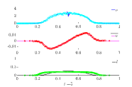
(a) $R=0.01,\varepsilon=10^{-3}$

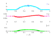
(b) $R=0.01,\varepsilon=10^{-4}$

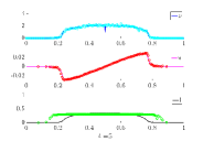
(c) $R=0.02,\varepsilon=10^{-4}$

Figure 1: Test 1D. Comparison between the numerical results of the macroscopic model (46c) with Dirichlet boundary conditions (continuous coloured lines) and of the microscopic stochastic process (4)-(9) ($o$ markers). Note that the average velocity and degree of leadership recovered from the microscopic model (o markers) are plotted only when the density is larger than $10^{-3}$, that corresponds, in the numerical integration of the microscopic model, to having more than 100 particles. A small numerical instability can be observed in the approximation of $\rho$ when the velocity changes sign and this is due to the upwind scheme used for the continuity equation.

5.3 Numerical tests in 2D

In this section we present the results of numerical simulations of the macroscopic model (46c) in a two-dimensional domain. The values of the model parameters are reported in Table 1.

5.3.1 Test 2Da: Turning and split

In this test we consider a single flock initially in a steady state, which starts moving and elongates. To this end we consider a square domain $\Omega=\left[0,2\right]\times\left[0,2\right]$, a final time $T=300$, and we set initial data as follows:

$$\rho(x,0) =\exp\left({-\frac{(x^{1}-C^{1}_{0})^{2}}{2\sigma_{0}^{2}}-\frac{(x^{2}-C^{2}_{0})^{2}}{2\sigma_{0}^{2}}}\right),$$

$$u(x,0) =0,$$

$$l(x,0) =0.9\exp\left({\frac{-(x^{1}-C^{1}_{1})^{2}}{2\sigma_{1}^{2}}-\frac{(x^{2}-C^{2}_{1})^{2}}{2\sigma_{1}^{2}}}\right)+0.8\exp\left({\frac{-(x^{1}-C^{1}_{2})^{2}}{2\sigma_{2}^{2}}-\frac{(x^{2}-C^{2}_{2})^{2}}{2\sigma_{2}^{2}}}\right),$$

for any $x=(x^{1},x^{2})\in\Omega$. Here $C_{0}=(C^{1}_{0},C^{2}_{0})=(1,1)$, $C_{1}=(C^{1}_{1},C^{2}_{1})=(0.8,0.8)$, $C_{2}=(C^{1}_{2},C^{2}_{2})=(1.3,1.3)$, $\sigma_{0}=\sqrt{0.03}$, $\sigma_{1}=\sigma_{2}=\sqrt{0.02}$. Figure 2 shows the initial conditions for $\rho$ and $l$. Note that at initial time the flock has null velocity, this means that the initial condition for $l$ will play a crucial role in the dynamics.

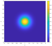
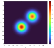
Figure 2: Test 2Da: Initial conditions for (a) $\rho$ and (b) $l$.

Boundary conditions are of Dirichlet type, with $\rho=u=l=0$. For the numerical approximation we set $\Delta x^{1}=\Delta x^{2}=0.025$ and $\Delta t=0.1$.

Figure 3 shows three snapshots of the evolution. At the beginning, the group starts moving in south-west direction, influenced by a higher degree of leadership in that region. After a while, we observe a turning behavior, with some agents which start moving in the opposite direction. As a result, the flock elongates and the interior density decreases.

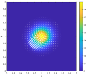
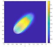
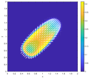
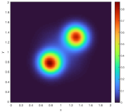
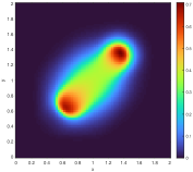
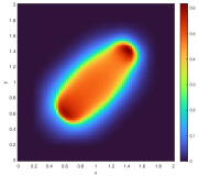
Figure 3: Test 2Da: evolution of $\rho$ (first line) and $l$ (second line) at time a),d) $t=10$, b),e) $t=90$, c),f) $t=210$ . White arrows describe the velocity field.

5.3.2 Test 2Db: Merge

In this test we simulate a scenario where two all-follower groups are initially distinct, then they merge interacting with each other. To this end, we consider a square domain $\Omega=\left[0,1\right]\times\left[0,1\right]$, a final time $T=350$, and we set initial data as follows:

$$\rho(x,0) =\exp\left({-\frac{(x^{1}-C^{1}_{3})^{2}}{2\sigma_{3}^{2}}-\frac{(x^{2}-C^{2}_{3})^{2}}{2\sigma_{3}^{2}}}\right)+\exp\left(-{\frac{(x^{1}-C^{1}_{4})^{2}}{2\sigma_{4}^{2}}-\frac{(x^{2}-C^{2}_{4})^{2}}{2\sigma_{4}^{2}}}\right),$$

$$u(x,0) =0,$$

$$l(x,0) =0,$$

for any $x=(x^{1},x^{2})\in\Omega$. Here $C_{3}=(C^{1}_{3},C^{2}_{3})=(0.4,0.7)$, $C_{4}=(C^{1}_{4},C^{2}_{4})=(0.6,0.3)$, $\sigma_{3}=\sigma_{4}=\sqrt{0.004}$. Initial density configuration is shown in Figure 4.

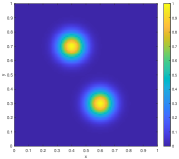
Figure 4: Test 2Db: initial condition for $\rho$.

Boundary conditions are of Dirichlet type, with $\rho=u=l=0$. The discretisation steps are $\Delta x^{1}=\Delta x^{2}=0.01$ and $\Delta t=0.2$.

Figure 5 shows three snapshots of the numerical simulation. At the beginning, the attraction force prevails and let the two groups merge. Meanwhile, the degree of leadership, initially equal to 0, increases and leaders appear. Once the two flocks merged, newly formed leaders establish a common direction of motion, heading the flock in the south-west direction.

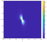
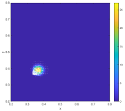
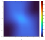
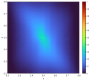
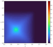
Figure 5: Test 2Db: evolution of $\rho$ (first line) and $l$ (second line) at time a),d) $t=20$, b),e) $t=40$, c),f) $t=180$ . White arrows describe the velocity field.

Figure 6 shows the same evolution with null Dirichlet boundary conditions for $\rho$ and $u$, but assuming $l\equiv 1$ at the border. It is interesting to compare the solutions of Figures 5 and 6 in order to quantify the impact of boundary conditions. It can be seen that the flock merge and find a common solution in both case, but the size of the final flock is quite different, proving that a nonnegligible effect of boundary conditions exists.

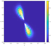
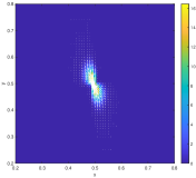
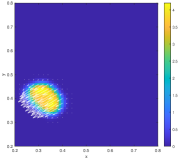
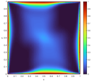
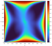
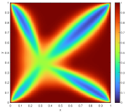
Figure 6: Test 2Db^′ (different boundary conditions for $l$): evolution of $\rho$ (first line) and $l$ (second line) at time a),d) $t=20$, b),e) $t=40$, c),f) $t=180$ . White arrows describe the velocity field.

5.3.3 Test 2Dc: Ring formation

In this test we consider the same initial and boundary conditions of Test 2Db (Figure 4), but we increase all the model parameters but $\alpha$ which remains equal, and $\gamma$ which is instead decreased. Doing this, we expect an accelerated dynamics of $l$ and a less impact of the attraction force. Result is shown in Figure 7. We observe that the two flocks still merge but remain less compressed than before. Moreover $l$ evolves faster toward to a mixed follower-leader status, which also spreads on all the domain due to the greater value of $R$.

More interesting, a ring formation appears, characterized by a high density of agents concentrated at the boundary of the flock. This configuration is well known and typically appears in all-to-all repulsion-attraction models [3, 42].

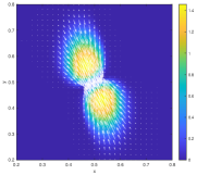
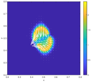
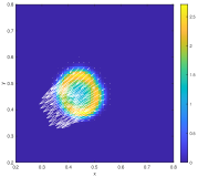
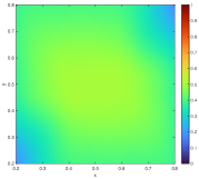
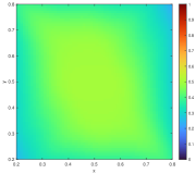
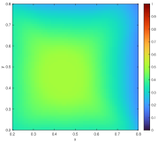
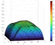
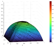
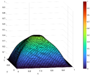
Figure 7: Test 2Dc: evolution of $\rho$ (first line) and $l$ (second and third lines) at time a),d),g) $t=20$, b),e),h) $t=48$, c),f),i) $t=100$ . White arrows describe the velocity field.

6 Conclusions

In this paper, we have proposed a Povzner-Boltzmann-type kinetic description of swarming dynamics with transient leadership and continuous leader-follower transitions relying on a simplified version of the microscopic dynamics described in [34]. The particles of the underlying multi-agent system feature a multi-variate microscopic state consisting of position, velocity and degree of leadership. The velocity and the degree of leadership change in consequence of binary interactions according to two independent processes, which are non-local in space. The resulting dynamics are largely non-conservative, the only conserved quantity being the mass. Non-locality and non-conservativeness pose two major theoretical issues in deriving a macroscopic description of the system through a hydrodynamic limit of the kinetic equation. To circumvent them, taking inspiration from the kinetic theory of nearly elastic granular gases [40, 59], we consider a regime of high interaction rates and small non-conservative contributions to the interactions. The combination of these two factors produces an aggregate description which still keeps track of the non-locality of the interactions, differently from a classical hyperbolic scaling of space and time in the kinetic equation, which would localise inevitably the mean effect of the interactions. As a consequence, we obtain a non-local macroscopic model in the form of a system of evolution equations for relevant statistical quantities formulated on the original spatial and temporal scales of the particle interactions. This means that, in principle, our analytical description is focused on the agents of the swarm also when it comes to aggregate dynamics, differently from the classical case of gas molecules, which instead disappear conceptually when the gas is described at the fluid scale in the hydrodynamic regime. This technique can be fruitfully adapted and extended to upscale consistently also different and possibly richer particle dynamics. As future perspective, we think that the leader/follower transition would be worth of further investigation in order to find the dynamics which better match the biological mechanisms, currently largely unexplored in both animal groups and human crowds.

Appendix A Strong form of the kinetic operators

The strong form of the collisional operator $Q^{v}(f,f)$ may be obtained by means of a change of variables in (11), taking advantage of the inverse binary collision:

$$\begin{aligned} {}^{\prime}\!v&=-\frac{1}{1-(1-\lambda)\beta}\left[v+\alpha\frac{x-x_{\ast}}{\left\lvert x-x_{\ast}\right\rvert^{2}}+(1-\lambda)\bigl{(}\beta{}^{\prime}\!v_{\ast}+\gamma(x_{\ast}-x)\bigr{)}\right]\\ {}^{\prime}\!v_{\ast}&=-\frac{1}{1-(1-\lambda_{\ast})\beta}\left[v_{\ast}+\alpha\frac{x_{\ast}-x}{\left\lvert x_{\ast}-x\right\rvert^{2}}+(1-\lambda_{\ast})\bigl{(}\beta{}^{\prime}\!v+\gamma(x-x_{\ast})\bigr{)}\right],\end{aligned}$$

where ${}^{\prime}\!v$, ${}^{\prime}\!v_{\ast}$ denote the pre-interaction velocities giving rise to the post-interaction velocities $v$, $v_{\ast}$. These are nothing but the inverse rules of (13)-(15). Then, after some algebraic manipulations, one gets

$$Q^{v}(f,f)(x,v,\lambda,t)=\int_{0}^{1}\int_{\mathbb{R}^{2d}}B(\left\lvert x_{\ast}-x\right\rvert)\left(\frac{f(x,{}^{\prime}\!v,\lambda,t)f(x_{\ast},{}^{\prime}\!v_{\ast},\lambda_{\ast},t)}{\left\lvert 1-\bigl{(}2-(\lambda+\lambda_{\ast})\bigr{)}\beta\right\rvert}-ff_{\ast}\right)\,dx_{\ast}\,dv_{\ast}\,d\lambda_{\ast}.$$ (52)

Analogously, the strong form of the collisional operator $Q^{\lambda}(f,f)$ may be obtained by means of a change of variables in (12), taking advantage of the inverse rule

$${}^{\prime}\!\lambda=1-\lambda,\qquad{}^{\prime}\!\lambda_{\ast}=1-\lambda_{\ast},$$

where ${}^{\prime}\!\lambda$, ${}^{\prime}\!\lambda_{\ast}$ are the pre-interaction degrees of leadership giving rise to the post-interaction ones $\lambda$, $\lambda_{\ast}$. Also in this case, these are the inverse rules of (14)-(16). The result is

$$Q^{\lambda}(f,f)(x,v,\lambda,t)=\int_{0}^{1}\int_{\mathbb{R}^{2d}}B(\left\lvert x_{\ast}-x\right\rvert)\bigl{(}f(x,v,{}^{\prime}\!\lambda,t)f(x_{\ast},v_{\ast},{}^{\prime}\!\lambda_{\ast},t)-ff_{\ast}\bigr{)}\,dx_{\ast}\,dv_{\ast}\,d\lambda_{\ast}.$$ (53)

To obtain the strong form of the operators $\bar{Q}^{v}(f,f)$ and $\mathcal{R}^{v}(f,f)$, cf. (22), (23), we proceed similarly. The inverse collision to (19) reads

$${}^{\prime}\!\bar{v}=\frac{1-p}{1-2p}v_{\ast}-\frac{p}{1-2p}v,\qquad{}^{\prime}\!\bar{v}_{\ast}=\frac{1-p}{1-2p}v-\frac{p}{1-2p}v_{\ast}$$

with $p:=\left(1-\frac{\lambda+\lambda_{\ast}}{2}\right)\beta_{0}\delta$, where ${}^{\prime}\!\bar{v}$, ${}^{\prime}\!\bar{v}_{\ast}$ denote the pre-interaction velocities giving rise to the post-interaction velocities $v$, $v_{\ast}$. Therefore, changing the variables in (22) produces

$$\bar{Q}^{v}(f,f)(x,v,\lambda,t)=\int_{0}^{1}\int_{\mathbb{R}^{2d}}B(\left\lvert x_{\ast}-x\right\rvert)\left(\frac{f(x,{}^{\prime}\!\bar{v},\lambda,t)f(x_{\ast},{}^{\prime}\!\bar{v}_{\ast},\lambda_{\ast},t)}{\left\lvert 1-\bigl{(}2-(\lambda+\lambda_{\ast})\bigr{)}\beta_{0}\delta\right\rvert}-ff_{\ast}\right)dx_{\ast}\,dv_{\ast}\,d\lambda_{\ast}.$$ (54)

The same change of variables in (23) yields instead

$$\left\langle\mathcal{R}^{v}(f,f),\,\varphi\right\rangle$$

$$=\int_{[0,\,1]^{2}}\int_{\mathbb{R}^{3d}}\Biggl{[}\frac{B(\left\lvert x_{\ast}-x\right\rvert)}{\left\lvert 1-\bigl{(}2-(\lambda+\lambda_{\ast})\bigr{)}\beta_{0}\delta\right\rvert}\left(\beta_{0}\frac{\lambda_{\ast}-\lambda}{2\bigl{(}1-(2-(\lambda+\lambda_{\ast}))\beta_{0}\delta\bigr{)}}(v-v_{\ast})\right.$$

$$\qquad\left.+\alpha_{0}\frac{x-x_{\ast}}{\left\lvert x-x_{\ast}\right\rvert^{2}}+\gamma_{0}(1-\lambda)(x_{\ast}-x)\right)\cdot\nabla_{v}\varphi(v,\lambda)f(x,{}^{\prime}\!\bar{v},\lambda,t)f(x_{\ast},{}^{\prime}\!\bar{v}_{\ast},\lambda_{\ast},t)\Biggr{]}\,dx_{\ast}\,dv\,dv_{\ast}\,d\lambda\,d\lambda_{\ast}$$

$$=-\int_{0}^{1}\int_{\mathbb{R}^{d}}\varphi(v,\lambda)\operatorname{div}_{v}\left[\int_{0}^{1}\int_{\mathbb{R}^{2d}}\frac{B(\left\lvert x_{\ast}-x\right\rvert)}{\left\lvert 1-\bigl{(}2-(\lambda+\lambda_{\ast})\bigr{)}\beta_{0}\delta\right\rvert}\left(\beta_{0}\frac{\lambda_{\ast}-\lambda}{2\bigl{(}1-(2-(\lambda+\lambda_{\ast}))\beta_{0}\delta\bigr{)}}(v-v_{\ast})\right.\right.$$

$$\qquad\left.\left.+\alpha_{0}\frac{x-x_{\ast}}{\left\lvert x-x_{\ast}\right\rvert^{2}}+\gamma_{0}(1-\lambda)(x_{\ast}-x)\right)f(x,{}^{\prime}\!\bar{v},\lambda,t)f(x_{\ast},{}^{\prime}\!\bar{v}_{\ast},\lambda_{\ast},t)\,dx_{\ast}\,dv_{\ast}\,d\lambda_{\ast}\right]dv\,d\lambda,$$

where the last passage follows from the divergence theorem, assuming further for convenience that $\varphi$ is compactly supported in $\mathbb{R}^{d}\times[0,\,1]$. Therefore:

$$\mathcal{R}^{v}(f,f)(x,v,\lambda,t)=\\ -\operatorname{div}_{v}\Biggl{[}\int_{0}^{1}\int_{\mathbb{R}^{2d}}\frac{B(\left\lvert x_{\ast}-x\right\rvert)}{\left\lvert 1-\bigl{(}2-(\lambda+\lambda_{\ast})\bigr{)}\beta_{0}\delta\right\rvert}\Biggl{(}\beta_{0}\frac{\lambda_{\ast}-\lambda}{2\bigl{(}1-(2-(\lambda+\lambda_{\ast}))\beta_{0}\delta\bigr{)}}(v-v_{\ast})\\ +\alpha_{0}\frac{x-x_{\ast}}{\left\lvert x-x_{\ast}\right\rvert^{2}}+\gamma_{0}(1-\lambda)(x_{\ast}-x)\Biggr{)}f(x,{}^{\prime}\!\bar{v},\lambda,t)f(x_{\ast},{}^{\prime}\!\bar{v}_{\ast},\lambda_{\ast},t)\,dx_{\ast}\,dv_{\ast}\,d\lambda_{\ast}\Biggr{]}.$$

The strong forms of the operators $\bar{Q}^{\lambda}(f,f)$ and $\mathcal{R}^{\lambda}(f,f)$, cf. (27), (28), can be obtained analogously starting from the inverse rules to (25). In particular, these are

$${}^{\prime}\!\bar{\lambda}=\frac{1-\nu}{1-2\nu}\lambda-\frac{\nu}{1-2\nu}\lambda_{\ast},\qquad{}^{\prime}\!\bar{\lambda}_{\ast}=\frac{1-\nu}{1-2\nu}\lambda_{\ast}-\frac{\nu}{1-2\nu}\lambda,$$

so that

$$\bar{Q}^{\lambda}(f,f)(x,v,\lambda,t)=\int_{0}^{1}\int_{\mathbb{R}^{2d}}B(\left\lvert x_{\ast}-x\right\rvert)\left(\frac{f(x,v,{}^{\prime}\!\bar{\lambda},t)f(x_{\ast},v_{\ast},{}^{\prime}\!\bar{\lambda}_{\ast},t)}{\left\lvert 1-2\nu\right\rvert}-ff_{\ast}\right)dx_{\ast}\,dv_{\ast}\,d\lambda_{\ast}$$

and

$$\mathcal{R}^{\lambda}(f,f)(x,v,\lambda,t)=\\ -\partial_{\lambda}\Biggl{[}\int_{0}^{1}\int_{\mathbb{R}^{2d}}\frac{B(\left\lvert x_{\ast}-x\right\rvert)}{\left\lvert 1-2\nu\right\rvert}\left(1-\frac{\nu}{1-2\nu}\lambda+\frac{3\nu-2}{1-2\nu}\lambda_{\ast}\right)\\ \times f(x,v,{}^{\prime}\!\bar{\lambda},t)f(x_{\ast},v_{\ast},{}^{\prime}\!\bar{\lambda}_{\ast},t)\,dx_{\ast}\,dv_{\ast}\,d\lambda_{\ast}\Biggr{]}.$$ (55)

References

- [1] P. Aceves-Sanchez, P. Degond, E. E. Keaveny, A. Manhart, S. Merino-Aceituno, and D. Peurichard. Large-scale dynamics of self-propelled particles moving through obstacles: Model derivation and pattern formation. Bull. Math. Biol., 82(10), 2020.
- [2] G. Albi, S. Almi, M. Morandotti, and F. Solombrino. Mean-field selective optimal control via transient leadership. Appl. Math. Optim., 85(2):22, 2022.
- [3] G. Albi, D. Balagué, J. A. Carrillo, and J. von Brecht. Stability analysis of flock and mill rings for second order models in swarming. SIAM J. Appl. Math., 74(3):794–818, 2014.
- [4] G. Albi, M. Bongini, E. Cristiani, and D. Kalise. Invisible control of self-organizing agents leaving unknown environments. SIAM J. Appl. Math., 76(4):1683–1710, 2016.
- [5] G. Albi, M. Bongini, F. Rossi, and F. Solombrino. Leader formation with mean-field birth and death models. Math. Models Methods Appl. Sci., 29(04):633–679, 2019.
- [6] G. Albi and F. Ferrarese. Kinetic description of swarming dynamics with topological interaction and emergent leaders. arXiv:2307.12044, 2023.
- [7] G. Albi and L. Pareschi. Modeling of self-organized systems interacting with a few individuals: from microscopic to macroscopic dynamics. Appl. Math. Lett., 26(4):397–401, 2013.
- [8] A. Attanasi, A. Cavagna, L. Del Castello, I. Giardina, T. S. Grigera, A. Jelić, S. Melillo, L. Parisi, O. Pohl, E. Shen, and M. Viale. Information transfer and behavioural inertia in starling flocks. Nat. Phys., 10:691–696, 2014.
- [9] A. Attanasi, A. Cavagna, L. Del Castello, I. Giardina, A. Jelic, S. Melillo, L. Parisi, O. Pohl, E. Shen, and M. Viale. Emergence of collective changes in travel direction of starling flocks from individual birds’ fluctuations. J. R. Soc. Interface, 12:20150319, 2015.
- [10] M. Ballerini, N. Cabibbo, R. Candelier, A. Cavagna, E. Cisbani, I. Giardina, V. Lecomte, A. Orlandi, G. Parisi, A. Procaccini, M. Viale, and V. Zdravkovic. Empirical investigation of starling flocks: A benchmark study in collective animal behaviour. Anim. Behav., 76(1):201–215, 2008.
- [11] M. Ballerini, N. Cabibbo, R. Candelier, A. Cavagna, E. Cisbani, I. Giardina, V. Lecomte, A. Orlandi, G. Parisi, A. Procaccini, M. Viale, and V. Zdravkovic. Interaction ruling animal collective behavior depends on topological rather than metric distance: Evidence from a field study. P. Natl. Acad. Sci. USA, 105(4):1232–1237, 2008.
- [12] D. Benedetto, P. Buttà, and E. Caglioti. Some aspects of the inertial spin model for flocks and related kinetic equations. Math. Models Methods Appl. Sci., 30(10):1987–2022, 2020.
- [13] S. Bernardi, R. Eftimie, and K. J. Painter. Leadership through influence: what mechanisms allow leaders to steer a swarm? Bull. Math. Biol., 83:69, 2021.
- [14] F. Bolley, J. A. Cañizo, and J. A. Carrillo. Stochastic mean-field limit: non-Lipschitz forces and swarming. Math. Models Methods Appl. Sci., 21(11):2179–2210, 2011.
- [15] M. Bongini and M. Fornasier. Sparse stabilization of dynamical systems driven by attraction and avoidance forces. Netw. Heterog. Media, 9(1):1–31, 2014.
- [16] A. Borzi and S. Wongkaew. Modeling and control through leadership of a refined flocking system. Math. Models Methods Appl. Sci., 25(02):255–282, 2015.
- [17] M. Bostan and J. A. Carrillo. Fluid models with phase transition for kinetic equations in swarming. Math. Models Methods Appl. Sci., 30(10):2023–2065, 2020.
- [18] S. Butail and M. Porfiri. Detecting switching leadership in collective motion. Chaos, 29(1):011102, 2019.
- [19] J. A. Cañizo, J. A. Carrillo, and J. Rosado. A well-posedness theory in measures for some kinetic models of collective motion. Math. Models Methods Appl. Sci., 21(03):515–539, 2011.
- [20] J. A. Carrillo, Y.-P. Choi, and M. Hauray. The derivation of swarming models: mean-field limit and Wasserstein distances. In A. Muntean and F. Toschi, editors, Collective Dynamics from Bacteria to Crowds: An Excursion Through Modeling, Analysis and Simulation, pages 1–46. Springer Vienna, Vienna, 2014.
- [21] J. A. Carrillo, Y.-P. Choi, M. Hauray, and S. Salem. Mean-field limit for collective behavior models with sharp sensitivity regions. J. Eur. Math. Soc., 21:121–161, 2019.
- [22] J. A. Carrillo, Y.-P. Choi, and S. P. Perez. A review on attractive–repulsive hydrodynamics for consensus in collective behavior. In N. Bellomo, P. Degond, and E. Tadmor, editors, Active Particles, Volume 1: Advances in Theory, Models, and Applications, pages 259–298. Springer International Publishing, Cham, 2017.
- [23] J. A. Carrillo, M. R. D’Orsogna, and V. Panferov. Double milling in self-propelled swarms from kinetic theory. Kinet. Relat. Models, 2(2):363–378, 2009.
- [24] J. A. Carrillo, M. Fornasier, G. Toscani, and F. Vecil. Particle, kinetic, and hydrodynamic models of swarming. In G. Naldi, L. Pareschi, and G. Toscani, editors, Mathematical Modeling of Collective Behavior in Socio-Economic and Life Sciences, pages 297–336. Birkhäuser Boston, Boston, 2010.
- [25] J. A. Carrillo, A. Wróblewska-Kamińska, and E. Zatorska. On long-time asymptotics for viscous hydrodynamic models of collective behavior with damping and nonlocal interactions. Math. Models Methods Appl. Sci., 29(01):31–63, 2019.
- [26] A. Cavagna, A. Cimarelli, I. Giardina, G. Parisi, R. Santagati, F. Stefanini, and R. Tavarone. From empirical data to inter-individual interactions: unveiling the rules of collective animal behavior. Math. Models Methods Appl. Sci., 20:1491–1510, 2010.
- [27] A. Cavagna, A. Culla, X. Feng, I. Giardina, T. S. Grigera, W. Kion-Crosby, S. Melillo, G. Pisegna, L. Postiglione, and P. Villegas. Marginal speed confinement resolves the conflict between correlation and control in collective behaviour. Nat. Commun., 13(1):2315, 2022.
- [28] A. Cavagna, L. Del Castello, I. Giardina, T. Grigera, A. Jelic, S. Melillo, T. Mora, L. Parisi, E. Silvestri, M. Viale, and A. M. Walczak. Flocking and turning: A new model for self-organized collective motion. J. Stat. Phys., 158:601–627, 2015.
- [29] A. Cavagna, S. M. Duarte Queirós, I. Giardina, F. Stefanini, and M. Viale. Diffusion of individual birds in starling flocks. Proc. R. Soc. B., 280:20122484, 2013.
- [30] D. Chen, T. Vicsek, X. Liu, T. Zhou, and H.-T. Zhang. Switching hierarchical leadership mechanism in homing flight of pigeon flocks. Europhys. Lett. EPL, 114(6):60008, 2016.
- [31] I. D. Couzin, J. Krause, N. R. Franks, and S. A. Levin. Effective leadership and decision-making in animal groups on the move. Nature, 433:513–516, 2005.
- [32] I. D. Couzin, J. Krause, R. James, G. D. Ruxton, and N. R. Franks. Collective memory and spatial sorting in animal groups. J. Theor. Biol., 218(1):1–11, 2002.
- [33] E. Cristiani, A. De Santo, and M. Menci. A generalized mean-field game model for the dynamics of pedestrians with limited predictive abilities. Commun. Math. Sci., 21(1):65–82, 2023.
- [34] E. Cristiani, M. Menci, M. Papi, and L. Brafman. An all-leader agent-based model for turning and flocking birds. J. Math. Biol., 83:45, 2021.
- [35] E. Cristiani, B. Piccoli, and A. Tosin. Multiscale modeling of granular flows with application to crowd dynamics. Multiscale Model. Simul., 9(1):155–182, 2011.
- [36] E. Cristiani, B. Piccoli, and A. Tosin. Multiscale modeling of pedestrian dynamics, volume 12. Springer, 2014.
- [37] F. Cucker and S. Smale. Emergent behavior in flocks. IEEE T. Automat. Contr., 52:852–862, 2007.
- [38] R. Eftimie. Hyperbolic and kinetic models for self-organised biological aggregations, volume 2232 of Lecture Notes in Mathematics, chapter Multi-dimensional transport equations, pages 153–193. Springer International Publishing, 2018.
- [39] M. Falcone and R. Ferretti. Semi-Lagrangian approximation schemes for linear and Hamilton-Jacobi equations. SIAM, 2013.
- [40] M. Fornasier, J. Haskovec, and G. Toscani. Fluid dynamic description of flocking via Povzner–Boltzmann equation. Phys. D, 240:21–31, 2011.
- [41] J. Herbert-Read. Collective behaviour: Leadership and learning in flocks. Curr. Biol., 25(23):R1127–R1129, 2015.
- [42] T. Kolokolnikov, H. Sun, D. Uminsky, and A. L. Bertozzi. Stability of ring patterns arising from two-dimensional particle interactions. Phys. Rev. E, 84:015203, 2011.
- [43] M. Lachowicz and M. Pulvirenti. A stochastic system of particles modelling the Euler equations. Arch. Rat. Mech. Anal., 109:81–93, 1990.
- [44] H. Ling, G. E. Mclvor, J. Westley, K. van der Vaart, J. Yin, R. T. Vaughan, A. Thornton, and N. T. Ouellette. Collective turns in jackdaw flocks: kinematics and information transfer. J. R. Soc. Interface, 16:20190450, 2019.
- [45] E. Loffredo, D. Venturelli, and I. Giardina. Collective response to local perturbations: how to evade threats without losing coherence. Phys. Biol., in press.
- [46] N. Loy and A. Tosin. Boltzmann-type equations for multi-agent systems with label switching. Kinet. Relat. Models, 14(5):867–894, 2021.
- [47] I. Markou. Invariance of velocity angles and flocking in the Inertial Spin model. Preprint, arXiv:2110.14388, 2021.
- [48] S. Motsch and E. Tadmor. A new model for self-organized dynamics and its flocking behavior. J. Stat. Phys., 144:923, 2011.
- [49] V. Mwaffo, J. Keshavan, T. L. Hedrick, and S. Humbert. Detecting intermittent switching leadership in coupled dynamical systems. Sci. Rep., 8:10338, 2018.
- [50] M. Papadopoulou, H. Hildenbrandt, D. W. E. Sankey, S. J. Portugal, and C. K. Hemelrijk. Emergence of splits and collective turns in pigeon flocks under predation. R. Soc. Open Sci., 9(2):211898, 2022.
- [51] L. Pareschi and G. Toscani. Interacting Multiagent Systems: Kinetic Equations and Monte Carlo Methods. Oxford University Press, Oxford, 2013.
- [52] B. Pettit, Z. Ákos, T. Vicsek, and D. Biro. Speed determines leadership and leadership determines learning during pigeon flocking. Curr. Biol., 25(23):3132–3137, 2015.
- [53] B. Piccoli and A. Tosin. Time-evolving measures and macroscopic modeling of pedestrian flow. Arch. Ration. Mech. Anal., 199:707–738, 2011.
- [54] H. Pomeroy and F. Heppner. Structure of turning in airborne Rock Dove (Columba Livia) flocks. The Auk, 109(2):256–267, 1992.
- [55] A. Y. Povzner. The Boltzmann equation in kinetic theory of gases. Amer. Math. Soc. Transl. Ser. 2, 47:193–216, 1962.
- [56] A. Procaccini, A. Orlandi, A. Cavagna, I. Giardina, F. Zoratto, D. Santucci, F. Chiarotti, C. K. Hemelrijk, E. Alleva, G. Parisi, and C. Carere. Propagating waves in starling, Sturnus vulgaris, flocks under predation. Anim. Behav., 82(4):759–765, 2011.
- [57] A. M. Reynolds, G. E. McIvor, A. Thornton, P. Yang, and N. T. Ouellette. Stochastic modelling of bird flocks: accounting for the cohesiveness of collective motion. J. R. Soc. Interface, 19(189):20210745, 2022.
- [58] D. J. T. Sumpter. The principles of collective animal behaviour. Phil. Trans. R. Soc. B, 361:5–22, 2006.
- [59] G. Toscani. Kinetic and hydrodynamic models of nearly elastic granular flows. In A. Jüngel, R. Manasevich, P. A. Markowich, and H. Shahgholian, editors, Nonlinear Differential Equation Models, Wien, 2004. Springer-Verlag.
- [60] T. Vicsek, A. Czirók, E. Ben-Jacob, I. Cohen, and O. Shochet. Novel type of phase transition in a system of self-driven particles. Phys. Rev. Lett., 75:1226–1229, 1995.
- [61] T. Vicsek and A. Zafeiris. Collective motion. Phys. Rep., 517(3):71–140, 2012.