Convolutional State Space Models for
Long-Range Spatiotemporal Modeling

Abstract

Effectively modeling long spatiotemporal sequences is challenging due to the need to model complex spatial correlations and long-range temporal dependencies simultaneously. ConvLSTMs attempt to address this by updating tensor-valued states with recurrent neural networks, but their sequential computation makes them slow to train. In contrast, Transformers can process an entire spatiotemporal sequence, compressed into tokens, in parallel. However, the cost of attention scales quadratically in length, limiting their scalability to longer sequences. Here, we address the challenges of prior methods and introduce convolutional state space models (ConvSSM) that combine the tensor modeling ideas of ConvLSTM with the long sequence modeling approaches of state space methods such as S4 and S5. First, we demonstrate how parallel scans can be applied to convolutional recurrences to achieve subquadratic parallelization and fast autoregressive generation. We then establish an equivalence between the dynamics of ConvSSMs and SSMs, which motivates parameterization and initialization strategies for modeling long-range dependencies. The result is ConvS5, an efficient ConvSSM variant for long-range spatiotemporal modeling. ConvS5 significantly outperforms Transformers and ConvLSTM on a long horizon Moving-MNIST experiment while training $3\times$ faster than ConvLSTM and generating samples $400\times$ faster than Transformers. In addition, ConvS5 matches or exceeds the performance of state-of-the-art methods on challenging DMLab, Minecraft and Habitat prediction benchmarks and enables new directions for modeling long spatiotemporal sequences.

1 Introduction

Developing methods that efficiently and effectively model long-range spatiotemporal dependencies is a challenging problem in machine learning. Whether predicting future video frames [1, 2], modeling traffic patterns [3, 4], or forecasting weather [5, 6], deep spatiotemporal modeling requires simultaneously capturing local spatial structure and long-range temporal dependencies. Although there has been progress in deep generative modeling of complex spatiotemporal data [7, 8, 9, 10, 11, 12], most prior work has only considered short sequences of 20-50 timesteps due to the costs of processing long spatiotemporal sequences. Recent work has begun considering sequences of hundreds to thousands of timesteps [13, 14, 15, 16]. As hardware and data collection of long spatiotemporal sequences continue to improve, new modeling approaches are required that scale efficiently with sequence length and effectively capture long-range dependencies.

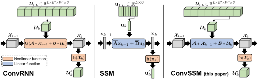
Figure 1: ConvRNNs [17, 18] (left) model spatiotemporal sequences using tensor-valued states, $\mathbfcal{X}_{k}$, and a nonlinear RNN update, $\mathbf{G}()$, that uses convolutions instead of matrix-vector multiplications. A position-wise nonlinear function, $\mathbf{h}()$, transforms the states into the output sequence. Deep SSMs [19, 20] (center) model vector-valued input sequences using a discretized linear SSM. The linear dynamics can be exploited to parallelize computations across the sequence and capture long-range dependencies. We introduce ConvSSMs (right) that model spatiotemporal data using tensor states, like ConvRNNs, and linear dynamics, like SSMs. We also introduce an efficient ConvSSM variant, ConvS5, that can be parallelized across the sequence with parallel scans, has fast autoregressive generation, and captures long-range dependencies.

Convolutional recurrent networks (ConvRNNs) such as ConvLSTM [17] and ConvGRU [18] are common approaches for spatiotemporal modeling. These methods encode the spatial information using tensor-structured states. The states are updated with recurrent neural network (RNN) equations that use convolutions instead of the matrix-vector multiplications in standard RNNs (e.g., LSTM/GRUs [21, 22]). This approach allows the RNN states to reflect the spatial structure of the data while simultaneously capturing temporal dynamics. ConvRNNs inherit both the benefits and the weaknesses of RNNs: they allow fast, stateful autoregressive generation and an unbounded context window, but they are slow to train due to their inherently sequential structure and can suffer from the vanishing/exploding gradient problem [23].

Transformer-based methods [9, 13, 14, 24, 25, 26, 27] operate on an entire sequence in parallel, avoiding these training challenges. Transformers typically require sophisticated compression schemes [28, 29, 30] to reduce the spatiotemporal sequence into tokens. Moreover, Transformers use an attention mechanism that has a bounded context window and whose computational complexity scales quadratically in sequence length for training and inference [31, 32]. More efficient Transformer methods improve on the complexity of attention [33, 34, 35, 36, 37, 38, 39], but these methods can fail on sequences with long-range dependencies [40, 13]. Some approaches combine Transformers with specialized training frameworks to address the attention costs [13]. However, recent work in deep state space models (SSMs) [19, 41, 42, 20, 43], like S4 [19] and S5 [20], has sought to overcome attention’s quadratic complexity while maintaining the parallelizability and performance of attention and the statefulness of RNNs. These SSM layers have proven to be effective in various domains such as speech [44], images [45] and video classification [45, 46]; reinforcement learning [47, 48]; forecasting [49] and language modeling [50, 51, 52, 53].

Inspired by modeling ideas from ConvRNNs and SSMs, we introduce convolutional state space models (ConvSSMs), which have a tensor-structured state like ConvRNNs but a continuous-time parameterization and linear state updates like SSM layers. See Figure 1. However, there are challenges to make this approach scalable and effective for modeling long-range spatiotemporal data. In this paper, we address these challenges and provide a rigorous framework that ensures both computational efficiency and modeling performance for spatiotemporal sequence modeling. First, we discuss computational efficiency and parallelization of ConvSSMs across the sequence for scalable training and fast inference. We show how to parallelize linear convolutional recurrences using a binary associative operator and demonstrate how this can be exploited to use parallel scans for subquadratic parallelization across the spatiotemporal sequence. We discuss both theoretical and practical considerations (Section 3.2) required to make this feasible and efficient. Next, we address how to capture long-range spatiotemporal dependencies. We develop a connection between the dynamics of SSMs and ConvSSMs (Section 3.3) and leverage this, in Section 3.4, to introduce a parameterization and initialization design that can capture long-range spatiotemporal dependencies.

As a result, we introduce ConvS5, a new spatiotemporal layer that is an efficient ConvSSM variant. It is parallelizable and overcomes difficulties during training (e.g., vanishing/exploding gradient problems) that traditional ConvRNN approaches experience. ConvS5 does not require compressing frames into tokens and provides an unbounded context. It also provides fast (constant time and memory per step) autoregressive generation compared to Transformers. ConvS5 significantly outperforms Transformers and ConvLSTM on a challenging long horizon Moving-MNIST [54] experiment requiring methods to train on 600 frames and generate up to 1,200 frames. In addition, ConvS5 trains $3\times$ faster than ConvLSTM on this task and generates samples $400\times$ faster than the Transformer. Finally, we show that ConvS5 matches or exceeds the performance of various state-of-the-art methods on challenging DMLab, Minecraft, and Habitat long-range video prediction benchmarks [13].

2 Background

This section provides the background necessary for ConvSSMs and ConvS5, introduced in Section 3.

2.1 Convolutional Recurrent Networks

Given a sequence of inputs $\mathbf{u}_{1:L}\in\mathbb{R}^{L\times U}$, an RNN updates its state, $\mathbf{x}_{k}\in\mathbb{R}^{P}$, using the state update equation $\mathbf{x}_{k}=\mathbf{F}(\mathbf{x}_{k-1},\mathbf{u_{k}})$, where $\mathbf{F}()$ is a nonlinear function. For example, a vanilla RNN can be represented (ignoring the bias term) as

$$\mathbf{x}_{k} =\mathrm{tanh}(\mathbf{A}\mathbf{x}_{k-1}+\mathbf{B}\mathbf{u_{k}})$$ (1)

with state matrix $\mathbf{A}\in\mathbb{R}^{P\times P}$, input matrix $\mathbf{B}\in\mathbb{R}^{P\times U}$ and $\mathrm{tanh}()$ applied elementwise. Other RNNs such as LSTM [21] and GRU [22] utilize more intricate formulations of $\mathbf{F}()$.

Convolutional recurrent neural networks [17, 18] (ConvRNNs) are designed to model spatiotemporal sequences by replacing the vector-valued states and inputs of traditional RNNs with tensors and substituting matrix-vector multiplications with convolutions. Given a length $L$ sequence of frames, $\mathbfcal{U}_{1:L}\in\mathbb{R}^{L\times H^{\prime}\times W^{\prime}\times U}$, with height $H^{\prime}$, width $W^{\prime}$ and $U$ features, a ConvRNN updates its state, $\mathbfcal{X}_{k}\in\mathbb{R}^{H\times W\times P}$, with a state update equation $\mathbfcal{X}_{k}=\mathbf{G}(\mathbfcal{X}_{k-1},\mathbfcal{U}_{k})$, where $\mathbf{G}()$ is a nonlinear function. Analogous to (1), we can express the state update equation for a vanilla ConvRNN as

$$\mathbfcal{X}_{k} =\mathrm{tanh}(\mathbfcal{A}*\mathbfcal{X}_{k-1}+\mathbfcal{B}*\mathbfcal{U}_{k}),$$ (2)

where $*$ is a spatial convolution operator with state kernel $\mathbfcal{A}\in\mathbb{R}^{P\times P\times k_{\mathcal{A}}\times k_{\mathcal{A}}}$ (using an [output features, input features, kernel height, kernel width] convention), input kernel $\mathbfcal{B}\in\mathbb{R}^{P\times U\times k_{\mathcal{B}}\times k_{\mathcal{B}}}$ and $\mathrm{tanh}()$ is applied elementwise. More complex updates such as ConvLSTM [17] and ConvGRU [18] are commonly used by making similar changes to the LSTM and GRU equations, respectively.

2.2 Deep State Space Models

This section briefly introduces deep SSMs such as S4 [19] and S5 [20] designed for modeling long sequences. The ConvS5 approach we introduce in Section 3 extends these ideas to the spatiotemporal domain.

Linear State Space Models

Given a continuous input signal $\mathbf{u}(t)\in\mathbb{R}^{U}$, a latent state $\mathbf{x}(t)\in\mathbb{R}^{P}$ and an output signal $\mathbf{y}(t)\in\mathbb{R}^{M}$, a continuous-time, linear SSM is defined using a differential equation:

$$\mathbf{x}^{\prime}(t)=\mathbf{A}\mathbf{x}(t)+\mathbf{B}\mathbf{u}(t),\quad\quad\mathbf{y}(t)=\mathbf{C}\mathbf{x}(t)+\mathbf{D}\mathbf{u}(t),$$ (3)

and is parameterized by a state matrix $\mathbf{A}\in\mathbb{R}^{P\times P}$, an input matrix $\mathbf{B}\in\mathbb{R}^{P\times U}$, an output matrix $\mathbf{C}\in\mathbb{R}^{M\times P}$ and a feedthrough matrix $\mathbf{D}\in\mathbb{R}^{M\times U}$. Given a sequence, $\mathbf{u}_{1:L}\in\mathbb{R}^{L\times U}$, the SSM can be discretized to define a discrete-time SSM

$$\mathbf{x}_{k}=\overline{\mathbf{A}}\mathbf{x}_{k-1}+\overline{\mathbf{B}}\mathbf{u}_{k},\quad\quad\mathbf{y}_{k}=\mathbf{C}\mathbf{x}_{k}+\mathbf{D}\mathbf{u}_{k},$$ (4)

where the discrete-time parameters are a function of the continuous-time parameters and a timescale parameter, $\Delta$. We define $\overline{\mathbf{A}}=\mathrm{DISCRETIZE_{A}}(\mathbf{A},\Delta)$ and $\overline{\mathbf{B}}=\mathrm{DISCRETIZE_{B}}(\mathbf{A},\mathbf{B},\Delta)$ where $\mathrm{DISCRETIZE}()$ is a discretization method such as Euler, bilinear or zero-order hold [55].

S4 and S5

Gu et al. [19] introduced the structured state space sequence (S4) layer to efficiently model long sequences. An S4 layer uses many continuous-time linear SSMs, an explicit discretization step with learnable timescale parameters, and position-wise nonlinear activation functions applied to the SSM outputs. Smith et al. [20] showed that with several architecture changes, the approach could be simplified and made more flexible by just using one SSM as in (3) and utilizing parallel scans. SSM layers, such as S4 and S5, take advantage of the fact that linear dynamics can be parallelized with subquadratic complexity in the sequence length. They can also be run sequentially as stateful RNNs for fast autoregressive generation. While a single SSM layer such as S4 or S5 has only linear dynamics, the nonlinear activations applied to the SSM outputs allow representing nonlinear systems by stacking multiple SSM layers [56, 57, 58].

SSM Parameterization and Initialization

Parameterization and initialization are crucial aspects that allow deep SSMs to capture long-range dependencies more effectively than prior attempts at linear RNNs [59, 60, 61]. The general setup includes continuous-time SSM parameters, explicit discretization with learnable timescale parameters, and state matrix initialization using structured matrices inspired by the HiPPO framework [62]. Prior research emphasizes the significance of these choices in achieving high performance on challenging long-range tasks [19, 20, 56, 57]. Recent work [57] has studied these parameterizations/initializations in more detail and provides insight into this setup’s favorable initial eigenvalue distributions and normalization effects.

2.3 Parallel Scans

We briefly introduce parallel scans, as used by S5, since they are important for parallelizing the ConvS5 method we introduce in Section 3. See Blelloch [63] for a more detailed review. A scan operation, given a binary associative operator $\bullet$ (i.e. $(a\bullet b)\bullet c=a\bullet(b\bullet c)$) and a sequence of $L$ elements $[a_{1},a_{2},...,a_{L}]$, yields the sequence: $[a_{1},\ (a_{1}\bullet a_{2}),\ ...,\ (a_{1}\bullet a_{2}\bullet...\bullet a_{L})]$.

Parallel scans use the fact that associative operators can be computed in any order. A parallel scan can be defined for the linear recurrence of the state update in (4) by forming the initial scan tuples $c_{k}=(c_{k,a},c_{k,b}):=(\overline{\mathbf{A}},\enspace\overline{\mathbf{B}}\mathbf{u}_{k})$ and utilizing a binary associative operator that takes two tuples $q_{i},q_{j}$ (either the initial tuples $c_{i},c_{j}$ or intermediate tuples) and produces a new tuple of the same type, $q_{i}\bullet q_{j}:=\left(q_{j,a}\odot q_{i,a},\enspace q_{j,a}\otimes q_{i,b}+q_{j,b}\right)$, where $\odot$ is matrix-matrix multiplication and $\otimes$ is matrix-vector multiplication. Given sufficient processors, the parallel scan computes the linear recurrence of (4) in $O(\log L)$ sequential steps (i.e., depth or span) [63].

3 Method

This section introduces convolutional state space models (ConvSSMs). We show how ConvSSMs can be parallelized with parallel scans. We then connect the dynamics of ConvSSMs to SSMs to motivate parameterization. Finally, we use these insights to introduce an efficient ConvSSM variant, ConvS5.

3.1 Convolutional State Space Models

Consider a continuous tensor-valued input $\mathbfcal{U}(t)\in\mathbb{R}^{H^{\prime}\times W^{\prime}\times U}$ with height $H^{\prime}$, width $W^{\prime}$, and number of input features $U$. We will define a continuous-time, linear convolutional state space model (ConvSSM) with state $\mathbfcal{X}(t)\in\mathbb{R}^{H\times W\times P}$, derivative $\mathbfcal{X}^{\prime}(t)\in\mathbb{R}^{H\times W\times P}$ and output $\mathbfcal{Y}(t)\in\mathbb{R}^{H\times W\times U}$, using a differential equation:

$$\mathbfcal{X}^{\prime}(t) =\mathbfcal{A}*\mathbfcal{X}(t)+\mathbfcal{B}*\mathbfcal{U}(t)$$ (5)

$$\mathbfcal{Y}(t) =\mathbfcal{C}*\mathbfcal{X}(t)+\mathbfcal{D}*\mathbfcal{U}(t)$$ (6)

where $*$ denotes the convolution operator, $\mathbfcal{A}\in\mathbb{R}^{P\times P\times k_{A}\times k_{A}}$ is the state kernel, $\mathbfcal{B}\in\mathbb{R}^{P\times U\times k_{B}\times k_{B}}$ is the input kernel, $\mathbfcal{C}\in\mathbb{R}^{U\times P\times k_{C}\times k_{C}}$ is the output kernel, and $\mathbfcal{D}\in\mathbb{R}^{U\times U\times k_{D}\times k_{D}}$ is the feedthrough kernel. For simplicity, we pad the convolution to ensure the same spatial resolution, $H\times W$, is maintained in the states and outputs. Similarly, given a sequence of $L$ inputs, $\mathbfcal{U}_{1:L}\in\mathbb{R}^{L\times H^{\prime}\times W^{\prime}\times U}$, we define a discrete-time convolutional state space model as

$$\mathbfcal{X}_{k} =\overline{\mathbfcal{A}}*\mathbfcal{X}_{k-1}+\overline{\mathbfcal{B}}*\mathbfcal{U}_{k}$$ (7)

$$\mathbfcal{Y}_{k} =\mathbfcal{C}*\mathbfcal{X}_{k}+\mathbfcal{D}*\mathbfcal{U}_{k}$$ (8)

where $\overline{\mathbfcal{A}}\in\mathbb{R}^{P\times P\times k_{A}\times k_{A}}$ and $\overline{\mathbfcal{B}}\in\mathbb{R}^{P\times U\times k_{B}\times k_{B}}$ denote that these kernels are in discrete-time.

3.2 Parallelizing Convolutional Recurrences

ConvS5 leverages parallel scans to efficiently parallelize the recurrence in (7). As discussed in Section 2.3, this requires a binary associative operator. Given that convolutions are associative, we show:

Proposition 1.

Consider a convolutional recurrence as in (7) and define initial parallel scan elements $c_{k}=(c_{k,a},c_{k,b}):=(\mathbf{\overline{\mathbfcal{A}}},\mathbf{\overline{\mathbfcal{B}}}*\mathbfcal{U}_{k})$. The binary operator $\circledast$, defined below, is associative.

$$q_{i}\circledast q_{j}:=(q_{j,a}\circ q_{i,a},\ q_{j,a}*q_{i,b}\ +\ q_{j,b}),$$ (9)

where $\circ$ denotes convolution of two kernels, $*$ denotes convolution and $+$ is elementwise addition.

Proof.

See Appendix A.1. ∎

Therefore, in theory, we can use this binary operator with a parallel scan to compute the recurrence in (7). However, the binary operator, $\circledast$, requires convolving two $k_{A}\times k_{A}$ resolution state kernels together. To maintain equivalence with the sequential scan, the resulting kernel will have resolution $2k_{a}-1\times 2k_{a}-1$. This implies that the state kernel will grow during the parallel scan computations for general kernels with a resolution greater than $1\times 1$. This allows the receptive field to grow in the time direction, a useful feature for capturing spatiotemporal context. However, this kernel growth is computationally infeasible for long sequences.

We address this challenge by taking further inspiration from deep SSMs. These methods opt for simple but computationally advantageous operations in the time direction (linear dynamics) and utilize more complex operations (nonlinear activations) in the depth direction of the model. These nonlinear activations allow a stack of SSM layers with linear dynamics to represent nonlinear systems. Analogously, we choose to use $1\times 1$ state kernels and perform pointwise state convolutions for the convolutional recurrence of (7). When we stack multiple layers of these ConvSSMs, the receptive field grows in the depth direction of the network and allows the stack of layers to capture the spatiotemporal context [64]. Computationally, we now have a construction that can be parallelized with subquadratic complexity with respect to the sequence length.

Proposition 2.

Given the effective inputs $\overline{\mathbfcal{B}}*\mathbfcal{U}_{1:L}\in\mathbb{R}^{L\times H\times W\times P}$ and a pointwise state kernel $\mathbfcal{A}\in\mathbb{R}^{P\times P\times 1\times 1}$, the computational cost of computing the convolutional recurrence in Equation 7 with a parallel scan is $\mathcal{O}\big{(}L(P^{3}+P^{2}HW)\big{)}$.

Proof.

See Appendix A.2. ∎

Further, the ConvS5 implementation introduced below admits a diagonalized parameterization that reduces this cost to $\mathcal{O}(LPHW)$. See Section 3.4 and Appendix B for more details.

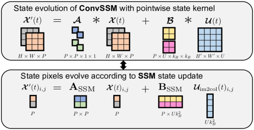
Figure 2: The dynamics of a ConvSSM with pointwise state kernel (top) can be equivalently viewed as the dynamics of an SSM (bottom). See Proposition 3. Each ConvSSM state pixel evolves according to an SSM state update with shared state matrix, $\mathbf{A}_{\mathrm{SSM}}$, and input matrix, $\mathbf{B}_{\mathrm{SSM}}$, that can be formed by reshaping the ConvSSM’s state kernel and input kernel. This allows leveraging parameterization insights from deep SSMs [19, 41, 42, 20, 57] to equip ConvS5 to model long-range dependencies.

3.3 Connection to State Space Models

Since the convolutions in (5-6) and (7-8) are linear operations, they can be described equivalently as matrix-vector multiplications by flattening the input and state tensors into vectors and using large, circulant matrices consisting of the kernel elements [65]. Thus, any ConvSSM can be described as a large SSM with a circulant dynamics matrix. However, we show here that the use of pointwise state kernels, as described in the previous section, provides an alternative SSM equivalence, which lends a special structure that can leverage the deep SSM parameterization/initialization ideas discussed in Section 2.2 for modeling long-range dependencies. We show that each pixel of the state, $\mathbfcal{X}(t)_{i,j}\in\mathbb{R}^{P}$, can be equivalently described as evolving according to a differential equation with a shared state matrix, $\mathbf{A}_{\mathrm{SSM}}$, and input matrix, $\mathbf{B}_{\mathrm{SSM}}$. See Figure 2.

Proposition 3.

Consider a ConvSSM state update as in (5) with pointwise state kernel $\mathbfcal{A}\in\mathbb{R}^{P\times P\times 1\times 1}$, input kernel $\mathbfcal{B}\in\mathbb{R}^{P\times U\times k_{B}\times k_{B}}$, and input  $\mathbfcal{U}(t)\in\mathbb{R}^{H^{\prime}\times W^{\prime}\times U}$. Let $\mathbfcal{U}_{\mathrm{im2col}}(t)\in\mathbb{R}^{H\times W\times Uk_{B}^{2}}$ be the reshaped result of applying the Image to Column (im2col) [66, 67] operation on the input $\mathbfcal{U}(t)$. Then the dynamics of each state pixel of (5), $\mathbfcal{X}(t)_{i,j}\in\mathbb{R}^{P}$, evolve according to the following differential equation

$$\mathbfcal{X}^{\prime}(t)_{i,j}=\mathbf{A}_{\mathrm{SSM}}\mathbfcal{X}(t)_{i,j}+\mathbf{B}_{\mathrm{SSM}}\mathbfcal{U}_{im2col}(t)_{i,j}$$ (10)

where the state matrix, $\mathbf{A}_{\mathrm{SSM}}\in\mathbb{R}^{P\times P}$, and input matrix, $\mathbf{B}_{\mathrm{SSM}}\in\mathbb{R}^{P\times(Uk_{B}^{2})}$, can be formed by reshaping the state kernel, $\mathbfcal{A}$, and input kernel, $\mathbfcal{B}$, respectively.

Proof.

See Appendix A.3. ∎

Thus, to endow these SSMs with the same favorable long-range dynamical properties as S4/S5 methods, we initialize $\mathbf{A}_{\mathrm{SSM}}$ with a HiPPO [62] inspired matrix and discretize with a learnable timescale parameter to obtain $\overline{\mathbf{A}}_{\mathrm{SSM}}$ and $\overline{\mathbf{B}}_{\mathrm{SSM}}$. Due to the equivalence of Proposition 3, we then reshape these matrices into the discrete ConvSSM state and input kernels of (7) to give the convolutional recurrence the same advantageous dynamical properties. We note that if the input, output and dynamics kernel widths are set to $1\times 1$, then the ConvSSM formulation is equivalent to "convolving" an SSM across each individual sequence of pixels in the spatiotemporal sequence (this also has connections to the temporal component of S4ND [45] when applied to videos). However, inspired by ConvRNNs, we observed improved performance when leveraging the more general convolutional structure the ConvSSM allows and increasing the input/output kernel sizes to allow local spatial features to be mixed in the dynamical system. See ablations discussed in Section 5.3.

3.4 Efficient ConvSSM for Long-Range Dependencies: ConvS5

Here, we introduce ConvS5, which combines ideas of parallelization of convolutional recurrences (Section 3.2) and the SSM connection (Section 3.3). ConvS5 is a ConvSSM that leverages parallel scans and deep SSM parameterization/initialization schemes. Given Proposition 3, we implicitly parameterize a pointwise state kernel, $\mathbfcal{A}\in\mathbb{R}^{P\times P\times 1\times 1}$ and input kernel $\mathbfcal{B}\in\mathbb{R}^{P\times U\times k_{B}\times k_{B}}$ in (5) using SSM parameters as used by S5 [20], $\mathbf{A}_{\mathrm{S5}}\in\mathbb{R}^{P\times P}$ and  $\mathbf{B}_{\mathrm{S5}}\in\mathbb{R}^{P\times(Uk_{B}^{2})}$. We discretize these S5 SSM parameters as discussed in Section 2.2 to give

$$\overline{\mathbf{A}}_{\mathrm{S5}}=\mathrm{DISCRETIZE_{A}}(\mathbf{A}_{\mathrm{S5}},\mathbf{\Delta}),\quad\quad\overline{\mathbf{B}}_{\mathrm{S5}}=\mathrm{DISCRETIZE_{B}}(\mathbf{A}_{\mathrm{S5}},\mathbf{B}_{\mathrm{S5}},\mathbf{\Delta}),$$ (11)

and then reshape to give the ConvS5 state update kernels:

$$\overline{\mathbf{A}}_{\mathrm{S5}}\in\mathbb{R}^{P\times P}\ \xrightarrow[]{\mathrm{reshape}}\ \overline{\mathbfcal{A}}_{\mathrm{ConvS5}}\in\mathbb{R}^{P\times P\times 1\times 1}$$ (12)

$$\overline{\mathbf{B}}_{\mathrm{S5}}\in\mathbb{R}^{P\times(Uk_{B}^{2})}\ \xrightarrow[]{\mathrm{reshape}}\ \overline{\mathbfcal{B}}_{\mathrm{ConvS5}}\in\mathbb{R}^{P\times U\times k_{B}\times k_{B}}.$$ (13)

We then run the discretized ConvSSM system of (7- 8), using parallel scans to compute the recurrence. In practice, this setup allows us to parameterize ConvS5 using a diagonalized parameterization [41, 42, 20] which reduces the cost of applying the parallel scan in Proposition 2 to $\mathcal{O}(LPHW)$. See Appendix B for a more detailed discussion of parameterization, initialization and discretization.

We define a ConvS5 layer as the combination of ConvS5 with a nonlinear function applied to the ConvS5 outputs. For example, for the experiments in this paper, we use ResNet[68] blocks for the nonlinear activations between layers. However, this is modular, and other choices such as ConvNext [69] or S4ND [45] blocks could easily be used as well. Finally, many ConvS5 layers can be stacked to form a deep spatiotemporal sequence model.

3.5 ConvS5 Properties

Refer to Table 1 for a comparison of computational complexity for Transformers, ConvRNNs and ConvS5. The parallel scans allow ConvS5 to be parallelized across the sequence like a Transformer but with cost only scaling linearly with the sequence length. In addition, ConvS5 is a stateful model like ConvRNNs, allowing fast autoregressive generation, extrapolation to different sequence lengths, and an unbounded context window. The connection with SSMs such as S5 derived in Section 3.3 allows for precisely specifying the initial dynamics to enable the modeling of long-range dependencies and to realize benefits from the unbounded context. Finally, the parallel scan of ConvS5 can allow leveraging the continuous-time parameterization to process irregularly sampled sequences in parallel. S5 achieves this by providing suitable spacing to the discretization operation [20], a procedure that ConvS5 can also use.

We have proposed a general ConvSSM structure that can be easily adapted to future innovations in the deep SSM literature. ConvS5’s parallel scan could be used to endow ConvS5 with time-varying dynamics such as the input-dependent dynamics shown to be beneficial in the Liquid-S4 [43] work. Multiple works [51, 52, 50, 53] proposed adding multiplicative gating to allow SSM-based methods to overcome some weaknesses on language modeling. Similar ideas could be useful to ConvSSMs for reasoning over long spatiotemporal sequences.

Table 1: Computational complexity of Transformers, ConvRNNS and ConvS5 with respect to sequence length. Metrics are inference cost (cost per step of autoregressive generation), cost per training step, and parallelization ability. ConvS5 combines the best of Transformers and ConvRNNs.

	Transformer	ConvRNNs	ConvS5
Inference	$\mathcal{O}(L)$	$\boldsymbol{\mathcal{O}(1)}$	$\boldsymbol{\mathcal{O}(1)}$
Training	$\mathcal{O}(L^{2})$	$\boldsymbol{\mathcal{O}(L)}$	$\boldsymbol{\mathcal{O}(L)}$
Parallelizable	Yes	No	Yes

4 Related Work

This work is most closely related to the ConvRNNs and deep SSMs already discussed. We note here that ConvRNNs have been used in numerous domains, including biomedical, robotics, traffic modeling and weather forecasting [70, 1, 71, 2, 3, 72, 73, 74, 75, 4, 76, 77]. In addition, many variants have been proposed [78, 79, 80, 81, 82, 83, 84, 64]. SSMs have been considered previously for video classification [46, 45, 85], however none addressed the challenging problem of generating long spatiotemporal sequences. S4ND [45] proposed applying separate S4 layers to each axis of an image or video, similar to a PixelRNN [86] approach, and then combining the results with an outer product. While that work mostly focused on images, they also show results for a short 30-frame video classification task. We note this approach could be complementary to ours and the S42D blocks could potentially be used to replace some of the ResNet blocks used as activations in our model. Other model architectures explored in the literature for spatiotemporal modeling include 3D convolution approaches [87, 88, 89], transformers, [9, 13, 14, 24, 25, 26, 27] and standard RNNs [16, 90]. Attempts to address the problem of modeling long spatiotemporal sequences have involved compressed representations [9, 91, 10, 92, 27, 29], training on sparse subsets of frames [15, 93, 8, 94, 95], temporal hierarchies [16], continuous-time neural representations [93, 95], training on different length sequences at different resolutions [96] and strided sampling [14, 97]. Of particular interest, Yan et al. [13] introduced the Temporally Consistent (TECO) Video Transformer, which achieved state-of-the-art performance on challenging 3D environment benchmarks designed to contain long-range dependencies [13]. This approach combines vector-quantized (VQ) latent dynamics with a MaskGit [98] dynamics prior, and several training tricks to model long videos.

5 Experiments

In Section 5.1, we present a long-horizon Moving-MNIST experiment to compare ConvRNNs, Transformers and ConvS5 directly. In Section 5.2, we evaluate ConvS5 on the challenging 3D environment benchmarks proposed in Yan et al. [13]. Finally, in Section 5.3, we discuss ablations that highlight the importance of ConvS5’s parameterization.

Table 2: Quantitative evaluation on the Moving-MNIST dataset [54]. Top: To evaluate, we condition on 100 frames, and then show results after generating 800 and 1200 frames. An expanded Table 6 is included in Appendix C with more results, error bars and ablations. Bold scores indicate the best performance and underlined scores indicate the second best performance. Bottom: Computational cost comparison for the 600 frame task. Compare to Table 1.

Trained on 300 frames $100\rightarrow 800$ $100\rightarrow 1200$ Method FVD $\downarrow$ PSNR $\uparrow$ SSIM $\uparrow$ LPIPS $\downarrow$ FVD $\downarrow$ PSNR $\uparrow$ SSIM $\uparrow$ LPIPS $\downarrow$ Transformer [24] $159$ $12.6$ $0.609$ $0.287$ $265$ $12.4$ $0.591$ $0.321$ Performer [33] $234$ $13.4$ $0.652$ $0.379$ $275$ $13.2$ $0.592$ $0.393$ CW-VAE [16] $\underline{104}$ $12.4$ $0.592$ $0.277$ $\mathbf{117}$ $12.3$ $0.585$ $0.286$ ConvLSTM [17] $128$ $\underline{15.0}$ $\underline{0.737}$ $\underline{0.169}$ $\underline{187}$ $\underline{14.1}$ $\mathbf{0.706}$ $\mathbf{0.203}$ ConvS5 $\hphantom{0}\mathbf{72}$ $\mathbf{16.0}$ $\mathbf{0.761}$ $\mathbf{0.156}$ $\underline{187}$ $\mathbf{14.5}$ $\underline{0.678}$ $\underline{0.230}$ Trained on 600 frames Transformer 0$\mathbf{42}$ $13.7$ $0.672$ $0.207$ $\hphantom{0}\underline{91}$ $13.1$ $0.631$ $0.252$ Performer 0$93$ $12.4$ $0.616$ $0.274$ $243$ $12.2$ $0.608$ $0.312$ CW-VAE 0$94$ $12.5$ $0.598$ $0.269$ $107$ $12.3$ $0.590$ $0.280$ ConvLSTM 0$91$ $\underline{15.5}$ $\underline{0.757}$ $\underline{0.149}$ $137$ $\underline{14.6}$ $\underline{0.727}$ $\underline{0.180}$ ConvS5 $\hphantom{0}\underline{47}$ $\mathbf{16.4}$ $\mathbf{0.788}$ $\mathbf{0.134}$ $\hphantom{0}\mathbf{71}$ $\mathbf{15.6}$ $\mathbf{0.763}$ $\mathbf{0.162}$ GFLOPS $\downarrow$ Train Step Time (s) $\downarrow$ Train Cost (V100 days) $\downarrow$ Sample Throughput (frames/s) $\uparrow$ Transformer $\underline{70}$ $\mathbf{0.77(1.0\times)}$ $\mathbf{50}$ 0.21 (1.0x) ConvLSTM $\mathbf{65}$ $3.0(3.9\times)$ $150$ $\mathbf{117\ (557\times)}$ ConvS5 $97$ $\underline{0.93(1.2\times)}$ $\mathbf{50}$ $\underline{90\ (429\times)}$

5.1 Long Horizon Moving-MNIST Generation

There are few existing benchmarks for training on and generating long spatiotemporal sequences. We develop a long-horizon Moving-MNIST [54] prediction task that requires training on 300-600 frames and accurately generating up to 1200 frames. This allows for a direct comparison of ConvS5, ConvRNNs and Transformers as well as an efficient attention alternative (Performer [33]) and CW-VAE [16], a temporally hierarchical RNN based method. We first train all models on 300 frames and then evaluate by conditioning on 100 frames before generating 1200. We repeat the evaluation after training on 600 frames. See Appendix D for more experiment details. We present the results after generating 800 and 1200 frames in Table 2. See Appendix C for randomly selected sample trajectories. ConvS5 achieves the best overall performance. When only trained on 300 frames, ConvLSTM and ConvS5 perform similarly when generating 1200 frames, and both outperform the Transformer. All methods benefit from training on the longer 600-frame sequence. However, the longer training length allows ConvS5 to significantly outperform the other methods across the metrics when generating 1200 frames.

In Table 2-bottom we revisit the theoretical properties of Table 1 and compare the empirical computational costs of the Transformer, ConvLSTM and ConvS5 on the 600 frame Moving-MNIST task. Although this specific ConvS5 configuration requires a few more FLOPs due to the convolution computations, ConvS5 is parallelizable during training (unlike ConvLSTM) and has fast autoregressive generation (unlike Transformer) — training 3x faster than ConvLSTM and generating samples 400x faster than Transformers.

Table 3: Quantitative evaluation on the DMLab long-range benchmark [13]. Results from Yan et al. [13] are indicated with $*$. Methods trained using the TECO [13] training framework are at the bottom of the table. TECO methods are slower to sample due to the MaskGit [98] procedure. The expanded Table 8 in Appendix C includes error bars and ablations.

	DMLab
Method	FVD $\downarrow$	PSNR $\uparrow$	SSIM $\uparrow$	LPIPS $\downarrow$	Sample Throughput (frames/s) $\uparrow$
FitVid* [90]	$176$	$12.0$	$0.356$	$0.491$	-
CW-VAE* [16]	$125$	$12.6$	$0.372$	$0.465$	-
Perceiver AR  * [39]	$\hphantom{0}96$	$11.2$	$0.304$	$0.487$	-
Latent FDM* [15]	$181$	$17.8$	$0.588$	$0.222$	-
Transformer [24]	$\hphantom{0}97$	$\underline{19.9}$	$0.619$	$\underline{0.123}$	$\hphantom{0}9$ ($1.0\times$)
Performer [33]	$\underline{80}$	$17.3$	$0.513$	$0.205$	$\hphantom{0}7$ ($0.8\times$)
S5 [20]	$221$	$19.3$	$\underline{0.641}$	$0.162$	$\underline{28}$ ($\underline{3.1\times}$)
ConvS5	$\mathbf{\hphantom{0}66}$	$\mathbf{23.2}$	$\mathbf{0.769}$	$\mathbf{0.079}$	$\mathbf{56}$ ($\mathbf{6.2\times})$
TECO-Transformer* [13]	$\hphantom{0}\mathbf{28}$	$\underline{22.4}$	$\underline{0.709}$	$0.155$	$16$ ($1.8\times$)
TECO-Transformer (our run)	$\hphantom{0}\mathbf{28}$	$21.6$	$0.696$	$\mathbf{0.082}$	$16$ ($1.8\times$)
TECO-S5	$\hphantom{0}35$	$20.1$	$0.687$	$0.143$	$\mathbf{21}$ ($\mathbf{2.3\times}$)
TECO-ConvS5	$\hphantom{0}\underline{31}$	$\mathbf{23.8}$	$\mathbf{0.803}$	$\underline{0.085}$	$\underline{18}$ ($\underline{2.0\times}$)

5.2 Long-range 3D Environment Benchmarks

Yan et al. [13] introduced a challenging video prediction benchmark specifically designed to contain long-range dependencies. This is one of the first comprehensive benchmarks for long-range spatiotemporal modeling and consists of 300 frame videos of agents randomly traversing 3D environments in DMLab [99], Minecraft [100], and Habitat [101] environments. See Appendix C for more experimental details and Appendix E for more details on each dataset.

We train models using the same $16\times 16$ vector-quantized (VQ) codes from the pretrained VQ-GANs [30] used for TECO and the other baselines in Yan et al. [13]. In addition to ConvS5 and the existing baselines, we also train a Transformer (without the TECO framework), Performer and S5. The S5 baseline serves as an ablation on ConvS5’s convolutional tensor-structured approach. Finally, since TECO is essentially a training framework (specialized for Transformers), we also use ConvS5 and S5 layers as a drop-in replacement for the Transformer in TECO. Therefore, we refer to the original version of TECO as TECO-Transformer, the ConvS5 version as TECO-ConvS5 and the S5 version as TECO-S5. See Appendix D for detailed information on training procedures, architectures, and hyperparameters.

DMLab

The results for DMLab are presented in Table 3. Of the methods trained without the TECO framework in the top section of Table 3, ConvS5 outperforms all baselines, including RNN [90, 16], efficient attention [39, 33] and diffusion [15] approaches. ConvS5 also has much faster autoregressive generation than the Transformer. ConvS5 significantly outperforms S5 on all metrics, pointing to the value of the convolutional structure of ConvS5.

For the models trained with the TECO framework, we see that TECO-ConvS5 achieves essentially the same FVD and LPIPS as TECO-Transformer, while significantly improving PSNR and SSIM. Note the sample speed comparisons are less dramatic in this setting since the MaskGit [98] sampling procedure is relatively slow. Still, the sample throughput of TECO-ConvS5 and TECO-S5 remains constant, while TECO-Transformer’s throughput decreases with sequence length.

Minecraft and Habitat

Table 4 presents the results on the Minecraft and Habitat benchmarks. On Minecraft, TECO-ConvS5 achieves the best FVD and performs comparably to TECO-Transformer on the other metrics, outperfoTarming all other baselines. On Habitat, TECO-ConvS5 is the only method to achieve a comparable FVD to TECO-Transformer, while outperforming it on PSNR and SSIM.

Table 4: Quantitative evaluation on the Minecraft and Habitat long-range benchmarks [13]. Results from Yan et al. [13] are indicated with $*$. See expanded Table 10 with error bars in Appendix C.

Minecraft Habitat Method FVD $\downarrow$ PSNR $\uparrow$ SSIM $\uparrow$ LPIPS $\downarrow$ FVD $\downarrow$ PSNR $\uparrow$ SSIM $\uparrow$ LPIPS $\downarrow$ FitVid* $956$ $13.0$ $0.343$ $0.519$ - - - - CW-VAE* $397$ $13.4$ $0.338$ $0.441$ - - - - Perceiver AR* $\hphantom{0}\underline{76}$ $13.2$ $0.323$ $0.441$ $164$ $\underline{12.8}$ $\mathbf{0.405}$ $0.676$ Latent FDM* $167$ $13.4$ $0.349$ $0.429$ $433$ $12.5$ $0.311$ $\mathbf{0.582}$ TECO-Transformer* $116$ $\mathbf{15.4}$ $\mathbf{0.381}$ $\mathbf{0.340}$ $\hphantom{0}\mathbf{76}$ $\underline{12.8}$ $0.363$ $\underline{0.604}$ TECO-ConvS5 $\hphantom{0}\mathbf{71}$ $\underline{14.8}$ $\underline{0.374}$ $\underline{0.355}$ $\hphantom{0}\underline{95}$ $\mathbf{12.9}$ $\underline{0.390}$ $0.632$

5.3 ConvS5 ablations

In Table 5 we present ablations on the convolutional structure of ConvS5. We compare different input and output kernel sizes for the ConvSSM and also compare the default ResNet activations to a channel mixing GLU [102] activation. Where possible, when reducing the sizes of the ConvSSM kernels, we redistribute parameters to the ResNet kernels or the GLU sizes to compare similar parameter counts. The results suggest more convolutional structure improves performance.

We also perform ablations to evaluate the importance of ConvS5’s deep SSM-inspired parameterization/initialization. We evaluate the performance of a ConvSSM with randomly initialized state kernel on both Moving-Mnist and DMLab. See Table 6 and Table 8 in Appendix C. We observe a degradation in performance in all settings for this ablation. This reflects prior results for deep SSMs [56, 19, 20, 57] and highlights the importance of the connection developed in Section 3.3.

Table 5: Ablations of ConvS5 convolutional structure for DMLab long-range benchmark dataset [13]. More convolutional structure improves overall performance. See expanded Table 9 in Appendix.

	DMLab
conv.	$\mathbfcal{B}$ kernel	$\mathbfcal{C}$ kernel	nonlinearity	FVD $\downarrow$	PSNR $\uparrow$	SSIM $\uparrow$	LPIPS $\downarrow$
x	-	-	GLU	${221}$	${19.3}$	${0.641}$	${0.162}$
o	$1\times 1$	$1\times 1$	GLU	$187$	$21.0$	$0.689$	$0.112$
o	$1\times 1$	$5\times 5$	GLU	$\hphantom{0}89$	$21.5$	$0.713$	$0.106$
o	$3\times 3$	$3\times 3$	GLU	$\hphantom{0}96$	$22.7$	$0.762$	$0.088$
o	$1\times 1$	$1\times 1$	ResNet	$\hphantom{0}81$	$23.0$	$0.767$	$0.083$
o	$1\times 1$	$3\times 3$	ResNet	$\hphantom{0}68$	$22.8$	$0.756$	$0.085$
o	$3\times 3$	$3\times 3$	ResNet	$\hphantom{0}\mathbf{67}$	$\mathbf{23.2}$	$\mathbf{0.769}$	$\mathbf{0.079}$

6 Discussion

This work introduces ConvS5, a new spatiotemporal modeling layer that combines the fast, stateful autoregressive generation of ConvRNNs with the ability to be parallelized across the sequence like Transformers. Its computational cost scales linearly with the sequence length, providing better scaling for longer spatiotemporal sequences. ConvS5 also leverages insights from deep SSMs to model long-range dependencies effectively.

We note that despite the ConvS5’s sub-quadratic scaling, it did not show significant training speedups over Transformers for sequence lengths of 300-600 frames. (See detailed run-time comparisons in Appendix C.) We expect ConvS5 to excel in training efficiency when applied to much longer spatiotemporal sequences where the quadratic scaling of Transformers dominates. We hope this work inspires the creation of longer spatiotemporal datasets and benchmarks. At the current sequence lengths, future optimizations of the parallel scan implementations in common deep learning frameworks will be helpful. In addition, the ResNet blocks used as the activations between ConvS5 layers could be replaced with efficient activations such as sparse convolutions [103] or S4ND [45].

An interesting future direction is to further utilize ConvS5’s continuous-time parameterization. Deep SSMs show strong performance when trained at one resolution and evaluated on another [19, 41, 42, 20, 43, 45]. In addition, S5 can leverage its parallel scan to effectively model irregularly sampled sequences [20]. ConvS5 can be used for such applications in the spatiotemporal domain [104, 93, 95]. Finally, ConvS5 is modular and flexible. We have demonstrated that ConvS5 works well as a drop-in replacement in the TECO [13] training framework specifically developed for Transformers. Due to its favorable properties, we expect ConvS5 to also serve as a building block of new approaches for modeling much longer spatiotemporal sequences and multimodal applications.

Appendix for: Convolutional State Space Models for Long-range Spatiotemporal Modeling

Contents:

• Appendix A: Propositions

• Appendix B: ConvS5 Details: Parameterization, Initialization, Discretization

• Appendix C: Supplementary Results

• Appendix D: Experiment Configurations

• Appendix E: Datasets

Appendix A Propositions

A.1 Parallel Scan for Convolutional Recurrences

Proposition 1.

Consider a convolutional recurrence as in (7) and define initial parallel scan elements $c_{k}=(c_{k,a},c_{k,b}):=(\mathbf{\overline{\mathbfcal{A}}},\mathbf{\overline{\mathbfcal{B}}}*\mathbfcal{U}_{k})$. The binary operator $\circledast$, defined below, is associative.

$$c_{i}\circledast c_{j}:=(c_{j,a}\circ c_{i,a},\ c_{j,a}*c_{i,b}\ +\ c_{j,b}),$$ (14)

where $\circ$ denotes convolution of two kernels, $*$ denotes convolution between a kernel and input, and $+$ is elementwise addition.

Proof.

Using that $\circ$ is associative and the companion operator of $*$, i.e. $(d\circ e)*f=d*(e*f)$ (see Blelloch [63], Section 1.4), we have:

$$(c_{i}\circledast c_{j})\circledast c_{k} =(c_{j,a}\circ c_{i,a},\ c_{j,a}*c_{i,b}\ +\ c_{j,b})\circledast(c_{k,a},c_{k,b})$$ (15)

$$=\bigg{(}c_{k,a}\circ(c_{j,a}\circ c_{i,a}),\enspace c_{k,a}*(c_{j,a}*c_{i,b}+c_{j,b})+c_{k,b}\bigg{)}$$ (16)

$$=\bigg{(}(c_{k,a}\circ c_{j,a})\circ c_{i,a},\enspace c_{k,a}*(c_{j,a}*c_{i,b})+c_{k,a}*c_{j,b}+c_{k,b}\bigg{)}$$ (17)

$$=\bigg{(}(c_{k,a}\circ c_{j,a})\circ c_{i,a},\enspace(c_{k,a}\circ c_{j,a})*c_{i,b}+c_{k,a}*c_{j,b}+c_{k,b}\bigg{)}$$ (18)

$$=c_{i}\circledast(c_{k,a}\circ c_{j,a},\enspace c_{k,a}*c_{j,b}+c_{k,b})$$ (19)

$$=c_{i}\circledast(c_{j}\circledast c_{k})$$ (20)

∎

A.2 Computational Cost of Parallel Scan for Convolutional Recurrences

Proposition 2.

Given the effective inputs $\overline{\mathbfcal{B}}*\mathbfcal{U}_{1:L}\in\mathbb{R}^{L\times H\times W\times P}$ and a pointwise state kernel $\mathbfcal{A}\in\mathbb{R}^{P\times P\times 1\times 1}$, the computational cost of computing the convolutional recurrence in Equation 7 with a parallel scan is $\mathcal{O}\big{(}L(P^{3}+P^{2}HW)\big{)}$.

Proof.

Following Blelloch [63], given a single processor, the cost of computing the recurrence sequentially using the binary operator $\circledast$ defined in Proposition 1 is $\mathcal{O}\big{(}L(T_{\circ}+T_{*}+T_{+})\big{)}$ where $T_{\circ}$ refers to the cost of convolving two kernels, $T_{*}$ is the cost of convolution between a kernel and input and $T_{+}$ is the cost of elementwise addition. The cost of elementwise addition is $T_{+}=\mathcal{O}(PHW)$. For state kernels with resolution $k_{A}$, $T_{\circ}=\mathcal{O}(P^{3}k_{A}^{4})$ and $T_{*}=\mathcal{O}(P^{2}k_{A}^{2}HW)$. For pointwise convolutions this becomes $T_{\circ}=\mathcal{O}(P^{3})$ and $T_{*}=\mathcal{O}(P^{2}HW)$. Thus, the cost of computing the recurrence sequentially using $\circledast$ is $\mathcal{O}\big{(}L(P^{3}+P^{2}HW)\big{)}$. Since there are work-efficient algorithms for parallel scans [105], the overall cost of the parallel scan is also $\mathcal{O}\big{(}L(P^{3}+P^{2}HW)\big{)}$. ∎

Note that ConvS5’s diagonalized parameterization discussed in Section 3.4 and Appendix B leads to $T_{\circ}=\mathcal{O}(P)$ and $T_{*}=\mathcal{O}(PHW)$. Therefore the cost of applying the parallel scan with ConvS5 is $\mathcal{O}(LPHW)$.

A.3 Connection Between ConvSSMs and SSMs

Proposition 3.

Consider a ConvSSM state update as in (5) with pointwise state kernel $\mathbfcal{A}\in\mathbb{R}^{P\times P\times 1\times 1}$, input kernel $\mathbfcal{B}\in\mathbb{R}^{P\times U\times k_{B}\times k_{B}}$, and input  $\mathbfcal{U}(t)\in\mathbb{R}^{H^{\prime}\times W^{\prime}\times U}$. Let $\mathbfcal{U}_{\mathrm{im2col}}(t)\in\mathbb{R}^{H\times W\times Uk_{B}^{2}}$ be the reshaped result of applying the Image to Column (im2col) [66, 67] operation on the input $\mathbfcal{U}(t)$. Then the dynamics of each state pixel of (5), $\mathbfcal{X}(t)_{i,j}\in\mathbb{R}^{P}$, evolve according to the following differential equation

$$\mathbfcal{X}^{\prime}(t)_{i,j}=\mathbf{A}_{\mathrm{SSM}}\mathbfcal{X}(t)_{i,j}+\mathbf{B}_{\mathrm{SSM}}\mathbfcal{U}_{im2col}(t)_{i,j}$$ (21)

where the state matrix, $\mathbf{A}_{\mathrm{SSM}}\in\mathbb{R}^{P\times P}$, and input matrix, $\mathbf{B}_{\mathrm{SSM}}\in\mathbb{R}^{P\times(Uk_{B}^{2})}$, can be formed by reshaping the state kernel, $\mathbfcal{A}$, and input kernel, $\mathbfcal{B}$, respectively.

Proof.

Let $\mathbf{U}_{\mathrm{im2col}}\in\mathbb{R}^{Uk_{b}^{2}\times HW}$ denote the result of performing the im2col operation on the input $\mathbfcal{U}(t)$ for convolution with the kernel $\mathbfcal{B}$. Reshape this matrix into the tensor $\mathbfcal{U}_{\mathrm{im2col}}(t)\in\mathbb{R}^{H\times W\times Uk_{b}^{2}}$. Reshape $\mathbfcal{U}_{\mathrm{im2col}}(t)$ once more into the tensor  $\mathbfcal{V}(t)\in\mathbb{R}^{H\times W\times U\times k_{B}\times k_{B}}$.

Now, we can write the evolution for the individual channels of each pixel, $\mathbfcal{X}^{\prime}(t)_{i,j,k}$, in (5) as

$$\mathbfcal{X}^{\prime}(t)_{i,j,k}=\sum_{l=0}^{P-1}\mathbfcal{A}_{k,l,0,0}\mathbfcal{X}(t)_{i,j,l}+\sum_{q=0}^{U-1}\sum_{m=0}^{k_{B}-1}\sum_{n=0}^{k_{B}-1}\mathbfcal{B}_{k,q,m,n}\mathbfcal{V}(t)_{i,j,q,m,n}.$$ (22)

Let $\mathbf{A}_{\mathrm{SSM}}\in\mathbb{R}^{P\times P}$ be a matrix with rows, $\mathbf{A}_{\mathrm{SSM},i}\in\mathbb{R}^{P}$, corresponding to a flattened version of the output features of $\mathbfcal{A}$, i.e. $\mathbfcal{A}_{i}\in\mathbb{R}^{P\times 1\times 1}$. Similarly, reshape $\mathbfcal{B}$ into a matrix $\mathbf{B}_{\mathrm{SSM}}\in\mathbb{R}^{P\times(Uk_{B}^{2})}$ where the rows, $\mathbf{B}_{\mathrm{SSM},i}\in\mathbb{R}^{Uk_{B}^{2}}$ correspond to a flattened version of the output features of $\mathbfcal{B}$, i.e. $\mathbfcal{B}_{i}\in\mathbb{R}^{U\times k_{B}\times k_{B}}$.

Then we can rewrite (22) equivalently as

$$\mathbfcal{X}^{\prime}(t)_{i,j,k} =\sum_{l=0}^{P-1}\mathbfcal{A}_{k,l,0,0}\mathbfcal{X}(t)_{i,j,l}+\sum_{q=0}^{U-1}\sum_{m=0}^{k_{B}-1}\sum_{n=0}^{k_{B}-1}\mathbfcal{B}_{k,q,m,n}\mathbfcal{V}(t)_{i,j,q,m,n}$$ (23)

$$=\sum_{l=0}^{P-1}\mathbf{A}_{\mathrm{SSM},k,l}\mathbfcal{X}(t)_{i,j,l}+\sum_{v=0}^{Uk_{B}^{2}-1}\mathbf{B}_{\mathrm{SSM},k,v}\mathbfcal{U}_{\mathrm{im2col}}(t)_{i,j,v}$$ (24)

$$=\mathbf{A}_{\mathrm{SSM},k}^{T}\mathbfcal{X}(t)_{i,j}+\mathbf{B}_{\mathrm{SSM},k}^{T}\mathbfcal{U}_{\mathrm{im2col}}(t)_{i,j}$$ (25)

∎

Appendix B ConvS5 Details: Parameterization, Discretization, Initialization

B.1 Background: S5

S5 Parameterization and Discretization

S5 [20] uses a diagonalized parameterization of the general SSM in (3).

Let $\mathbf{A}_{\mathrm{S5}}=\mathbf{V}\mathbf{\Lambda}_{\mathrm{S5}}\mathbf{V^{-1}}\in\mathbb{R}^{P\times P}$ where $\mathbf{\Lambda}_{\mathrm{S5}}\in\mathbb{C}^{P\times P}$ is a complex-valued diagonal matrix and $\mathbf{V}\in\mathbb{C}^{P\times P}$ corresponds to the eigenvectors. Defining $\tilde{\mathbf{x}}(t)=\mathbf{V}^{-1}\mathbf{x}(t)$, $\tilde{\mathbf{B}}=\mathbf{V}^{-1}\mathbf{B}$, and $\tilde{\mathbf{C}}=\mathbf{C}\mathbf{V}$ we can reparameterize the SSM of (3) as the diagonalized system:

$$\dfrac{\mathrm{d}\tilde{\mathbf{x}}(t)}{\mathrm{d}t}=\mathbf{\Lambda}_{\mathrm{S5}}\tilde{\mathbf{x}}(t)+\tilde{\mathbf{B}}\mathbf{u}(t),\quad\quad\mathbf{y}(t) =\tilde{\mathbf{C}}\tilde{\mathbf{x}}(t)+\mathbf{D}\mathbf{u}(t).$$ (26)

S5 uses learnable timescale parameters $\mathbf{\Delta}\in\mathbb{R}^{P}$ and the following zero-order hold (ZOH) disretization:

$$\overline{\mathbf{\Lambda}}_{\mathrm{S5}} =\mathrm{DISCRETIZE_{A}}(\mathbf{\Lambda}_{\mathrm{S5}},\mathbf{\Delta}):=e^{\mathbf{\Lambda}_{\mathrm{S5}}\mathbf{\Delta}}$$ (27)

$$\overline{\mathbf{B}}_{\mathrm{S5}} =\mathrm{DISCRETIZE_{B}}(\mathbf{\Lambda}_{\mathrm{S5}},\tilde{\mathbf{B}},\mathbf{\Delta}):=\mathbf{\Lambda}_{\mathrm{S5}}^{-1}(\overline{\mathbf{\Lambda}}_{\mathrm{S5}}-\mathbf{I})\tilde{\mathbf{B}}\$$ (28)

S5 Initialization

S5 initializes its state matrix by diagonalizing $\mathbf{A}_{\mathrm{S5}}$ as defined here:

$$\mathbf{A}_{\mathrm{S5}_{nk}} =-\begin{cases}(n+\frac{1}{2})^{1/2}(k+\frac{1}{2})^{1/2},&n>k\\ \frac{1}{2},&n=k\\ (n+\frac{1}{2})^{1/2}(k+\frac{1}{2})^{1/2},&n<k\end{cases}.$$ (29)

This matrix is the normal part of the normal plus low-rank HiPPO-LegS matrix from the HiPPO framework [62] for online function approximation. S4 originally initialized its single-input, single-output (SISO) SSMs with a representation of the full HiPPO-LegS matrix. This was shown to be approximating long-range dependencies at initialization with respect to an infinitely long, exponentially-decaying measure [106]. Gupta et al. [41] empirically showed that the low-rank terms could be removed without impacting performance. Gu et al. [42] showed that in the limit of infinite state dimension, the linear, single-input ODE with this normal approximation to the HiPPO-LegS matrix produces the same dynamics as the linear, single-input ODE with the full HiPPO-LegS matrix. The S5 work extended these findings to the multi-input SSM setting [20].

Importance of SSM Parameterization, Discretization and Initialization

Prior research has highlighted the importance of parameterization, discretization and initialization choices of deep SSM methods through ablations and analysis [56, 19, 42, 20, 57]. Concurrent work from Orvieto et al. [57] provides particular insight into the favorable initial eigenvalue distributions provided by initializing with HiPPO-inspired matrices as well as an important normalization effect provided by the explicit discretization procedure. They also introduce a purely discrete-time parameterization that can perform similarly to the continuous-time discretization of S4 and S5. However, their parameterization practically ends up quite similar to the equations of (27-28). We choose to use the continuous-time parameterization of S5 for the implicit parameterization of ConvS5 since it can also be leveraged for zero-shot resolution changes [19, 20, 45] and processing irregularly sampled time-series in parallel [20]. However, due to Proposition 3, other long-range SSM parameterization strategies can also be used, such as in Orvieto et al. [57] or potential future innovations.

B.2 ConvS5 Diagonalization

We leverage S5’s diagonalized parameterization to reduce the cost of the parallel scan of ConvS5.

Concretely, we initialize $\mathbf{A}_{\mathrm{S5}}$ as in (29) and diagonalize as $\mathbf{A}_{\mathrm{S5}}=\mathbf{V}\mathbf{\Lambda}_{\mathrm{S5}}\mathbf{V^{-1}}$. To apply ConvS5, we compute $\overline{\mathbf{\Lambda}}_{\mathrm{S5}}$ and $\overline{\mathbf{B}}_{\mathrm{S5}}$ using (27-28), and then form the ConvS5 state and input kernels:

$$\overline{\mathbf{\Lambda}}_{\mathrm{S5}}\in\mathbb{R}^{P\times P}\ \xrightarrow[]{\mathrm{reshape}}\ \overline{\mathbfcal{A}}_{\mathrm{ConvS5}}\in\mathbb{R}^{P\times P\times 1\times 1}$$ (30)

$$\overline{\mathbf{B}}_{\mathrm{S5}}\in\mathbb{R}^{P\times(Uk_{B}^{2})}\ \xrightarrow[]{\mathrm{reshape}}\ \overline{\mathbfcal{B}}_{\mathrm{ConvS5}}\in\mathbb{R}^{P\times U\times k_{B}\times k_{B}}.$$ (31)

See Listing 1 for an example of the core implementation. Note, the state kernel $\overline{\mathbfcal{A}}_{\mathrm{ConvS5}}$ is "diagonalized" in the sense that all entries in the state kernel are zero except $\overline{\mathbfcal{A}}_{\mathrm{ConvS5},i,i}=\overline{\mathbf{\Lambda}}_{\mathrm{S5},i,i}\ \ \forall i\in[P]$. This means that the pointwise convolutions reduce to channel-wise multiplications. However, this does not reduce expressivity compared to a full pointwise convolution. This is because, given the ConvSSM to SSM equivalence of Proposition 3 and the use of complex-valued kernels, the diagonalization maintains expressivity since almost all SSMs are diagonalizable [41, 42], which follows from the well-known fact that almost all square matrices diagonalize over the complex plane.

⬇

1import jax

2import jax.numpy as np

3from ConvSSM_helpers import discretize, Conv2D, ResNet_Block

4parallel_scan = jax.lax.associative_scan

5

6def apply_ConvS5_layer(A, B, B_shape, C_kernel, log_Delta, resnet_params, us, x0):

7 """Compute the outputs of ConvS5 layer given input sequence.

8 Args:

9 A (complex64): S5 state matrix (P,)

10 B (complex64): S5 input matrix (P,Uk_B^2)

11 B_shape (tuple): shape of B_kernel

12 C_kernel (complex64) output kernel (U,P,k_C,k_C)

13 log_Delta (float32): learnable timescale params (P,)

14 resnet_params (dict): ResNet block params

15 us (float32): input sequence of features (L,bsz,H,W,U)

16 x0 (complex64): initial state (bsz,H,W,P)

17 Returns:

18 outputs (float32): the ConvS5 layer outputs (L,bsz,H,W,U)

19 x_L (complex64): the last state of the ConvSSM (bsz,H,W,P)

20 """

21 # Discretize and reshape ConvS5 state and input kernels

22 P, U, k_B = B_shape

23 A_bar, B_bar = discretize(A, B, np.exp(log_Delta))

24 A_kernel = A_bar # already correct shape due to diagonalization

25 B_kernel = B_bar.reshape(P, U, k_B, k_B)

26

27 # Apply ConvS5

28 ys, xs = apply_ConvS5(A_kernel, B_kernel, C_kernel, us, x0)

29

30 # Apply ResNet activation function

31 outputs = jax.vmap(ResNet_Block, axis=(None,0))(resnet_params, ys)

32 return outputs, xs[-1]

33

34def apply_ConvS5(A_kernel, B_kernel, C_kernel, us, x0):

35 """Compute the output sequence of the convolutional SSM

36 given the input sequence using a parallel scan.

37 Computes x_k = A * x_{k-1} + B * u_k

38 y_k = C * x_k

39 where * is a convolution operator.

40 Args:

41 A_kernel (complex64): state kernel (P,)

42 B_kernel (complex64): input kernel (P,U,k_B,k_B)

43 C_kernel (complex64): output kernel (U,P,k_C,k_C)

44 us (float32): input sequence (L,bsz,H,W,U)

45 x0 (complex64): initial state (bsz,H,W,P)

46 Returns:

47 ys (float32): the convS5 outputs (L,bsz,H,W,U)

48 x_L (complex64): the last state (bsz,H,W,P)

49 """

50 # Compute initial scan elements

51 As = np.repeat(A_kernel[None, ...], us.shape[0], axis=0)

52 Bus = jax.vmap(Conv2D)(B_kernel, np.complex64(us))

53 Bus = Bus.at[0].add(np.expand_dims(A_bar, (0, 1, 2)) * x0)

54

55 # Convolutional recurrence with parallel scan

56 _, xs = parallel_scan(conv_binary_operator, (As, Bus))

57

58 # Compute ConvS5 outputs

59 ys = jax.vmap(Conv2D)(C_kernel, xs).real

60 return ys, xs

61

62def conv_binary_operator(q_i, q_j):

63 """Binary operator for convolutional recurrence

64 with "diagonalized" 1X1 state kernels.

65 Args:

66 q_i, q_j (tuples): scan elements q_i=(A_i, BU_i) where

67 A_i (complex64) is state kernel (P,)

68 BU_i (complex64) is effective input (bsz,H,W,P)

69 Returns:

70 output tuple q_i \circledast q_j

71 """

72 A_i, BU_i = q_i

73 A_j, BU_j = q_j

74 # Convolve "diagonal" 1X1 kernels

75 AA = A_j * A_i

76 # Convolve "diagonal" A_j with BU_i

77 A_jBU_i = np.expand_dims(A_j, (0, 1, 2)) * BU_i

78 return AA, A_jBU_i + BU_j

Listing 1: JAX implementation of core code to apply a single ConvS5 layer to a batch of spatiotemporal input sequences.

Appendix C Supplementary Results

We include expanded tables and sample trajectories from the experiments in the main paper. Sample videos can be found at:

https://sites.google.com/view/convssm.

C.1 Moving-MNIST

Table 6: Full results on the Moving-MNIST dataset [54]. For the top table, all models are trained on 300 frames. For the bottom table, all models are trained on 600 frames. The evaluation task is to condition on 100 frames, and then generate forward 400, 800 and 1200 frames. ConvSSM (ablation) is performed by randomly initializing the state kernel (see Section 5.3 and Appendix D.4).

Trained on 300 frames $100\rightarrow 400$ $100\rightarrow 800$ $100\rightarrow 1200$ Method Params FVD $\downarrow$ PSNR $\uparrow$ SSIM $\uparrow$ LPIPS $\downarrow$ FVD $\downarrow$ PSNR $\uparrow$ SSIM $\uparrow$ LPIPS $\downarrow$ FVD $\downarrow$ PSNR $\uparrow$ SSIM $\uparrow$ LPIPS $\downarrow$ Transformer 164M $73\pm 3$ $13.5\pm 0.1$ $0.669\pm 0.002$ $0.213\pm 0.003$ $159\pm 7$ $12.6\pm 0.1$ $0.609\pm 0.002$ $0.287\pm 0.001$ $265\pm 8$ $12.4\pm 0.1$ $0.591\pm 0.002$ $0.321\pm 0.002$ Performer 164M $111\pm 9$ $13.4\pm 0.1$ $0.653\pm 0.002$ $0.288\pm 0.001$ $234\pm 1$ $13.4\pm 0.1$ $0.652\pm 0.006$ $0.379\pm 0.002$ $275\pm 5$ $13.2\pm 0.1$ $0.592\pm 0.001$ $0.393\pm 0.001$ CW-VAE 20M $\hphantom{0}78\pm 1$ $12.7\pm 0.1$ $0.611\pm 0.002$ $0.254\pm 0.001$ $104\pm 2$ $12.4\pm 0.1$ $0.592\pm 0.002$ $0.277\pm 0.002$ $\mathbf{117\pm 2}$ $12.3\pm 0.1$ $0.585\pm 0.002$ $0.286\pm 0.001$ ConvLSTM 20M $\hphantom{0}\underline{57\pm 3}$ $\underline{16.9\pm 0.2}$ $\underline{0.796\pm 0.004}$ $\underline{0.113\pm 0.002}$ $\underline{128\pm 4}$ $\underline{15.0\pm 0.1}$ $\underline{0.737\pm 0.003}$ $\underline{0.169\pm 0.001}$ $\underline{187\pm 6}$ $\underline{14.1\pm 0.1}$ $\mathbf{0.706\pm 0.003}$ $\mathbf{0.203\pm 0.001}$ ConvSSM (ablation) 20M $\hphantom{0}67\pm 3$ $15.5\pm 0.1$ $0.742\pm 0.001$ $0.168\pm 0.001$ $287\pm 5$ $13.6\pm 0.1$ $0.577\pm 0.001$ $0.293\pm 0.001$ $511\pm 8$ $13.3\pm 0.1$ $0.515\pm 0.001$ $0.348\pm 0.001$ ConvS5 20M $\hphantom{0}\mathbf{26\pm 1}$ $\mathbf{18.1\pm 0.1}$ $\mathbf{0.830\pm 0.003}$ $\mathbf{0.094\pm 0.002}$ $\hphantom{0}\mathbf{72\pm 3}$ $\mathbf{16.0\pm 0.1}$ $\mathbf{0.761\pm 0.005}$ $\mathbf{0.156\pm 0.003}$ $\underline{187\pm 5}$ $\mathbf{14.5\pm 0.1}$ $\underline{0.678\pm 0.003}$ $\underline{0.230\pm 0.004}$ Trained on 600 frames $100\rightarrow 400$ $100\rightarrow 800$ $100\rightarrow 1200$ Method Params FVD $\downarrow$ PSNR $\uparrow$ SSIM $\uparrow$ LPIPS $\downarrow$ FVD $\downarrow$ PSNR $\uparrow$ SSIM $\uparrow$ LPIPS $\downarrow$ FVD $\downarrow$ PSNR $\uparrow$ SSIM $\uparrow$ LPIPS $\downarrow$ Transformer 164M $\hphantom{0}\mathbf{21\pm 1}$ $15.0\pm 0.1$ $0.741\pm 0.002$ $0.138\pm 0.001$ 0$\mathbf{42\pm 2}$ $13.7\pm 0.1$ $0.672\pm 0.002$ $0.207\pm 0.003$ $\hphantom{0}\underline{91\pm 6}$ $13.1\pm 0.1$ $0.631\pm 0.004$ $0.252\pm 0.002$ Performer 164M $\hphantom{0}27\pm 1$ $13.1\pm 0.1$ $0.654\pm 0.004$ $0.206\pm 0.001$ 0$93\pm 5$ $12.4\pm 0.1$ $0.616\pm 0.002$ $0.274\pm 0.001$ $\hphantom{0}243\pm 7$ $12.2\pm 0.1$ $0.608\pm 0.001$ $0.312\pm 0.002$ CW-VAE 20M $\hphantom{0}73\pm 2$ $12.9\pm 0.1$ $0.621\pm 0.004$ $0.242\pm 0.001$ $\hphantom{0}94\pm 3$ $12.5\pm 0.9$ $0.598\pm 0.004$ $0.269\pm 0.001$ $107\pm 2$ $12.3\pm 0.1$ $0.590\pm 0.004$ $0.280\pm 0.002$ ConvLSTM 20M $\hphantom{0}39\pm 5$ $\underline{17.3\pm 0.2}$ $\underline{0.812\pm 0.005}$ $\underline{0.100\pm 0.003}$ 0$91\pm 7$ $\underline{15.5\pm 0.2}$ $\underline{0.757\pm 0.005}$ $\underline{0.149\pm 0.003}$ $137\pm 9$ $\underline{14.6\pm 0.1}$ $\underline{0.727\pm 0.004}$ $\underline{0.180\pm 0.003}$ ConvSSM (ablation) 20M $\hphantom{0}81\pm 6$ $15.5\pm 0.1$ $0.743\pm 0.002$ $0.163\pm 0.003$ $145\pm 8$ $14.3\pm 0.1$ $0.696\pm 0.002$ $0.218\pm 0.002$ $215\pm 9$ $13.4\pm 0.1$ $0.614\pm 0.001$ $0.287\pm 0.001$ ConvS5 20M $\hphantom{0}\underline{23\pm 3}$ $\mathbf{18.1\pm 0.1}$ $\mathbf{0.832\pm 0.003}$ $\mathbf{0.092\pm 0.003}$ $\hphantom{0}\underline{47\pm 7}$ $\mathbf{16.4\pm 0.1}$ $\mathbf{0.788\pm 0.002}$ $\mathbf{0.134\pm 0.003}$ $\hphantom{0}\mathbf{71\pm 9}$ $\mathbf{15.6\pm 0.1}$ $\mathbf{0.763\pm 0.002}$ $\mathbf{0.162\pm 0.003}$

Table 7: Model runtime comparison for Moving-MNIST results in Table 6. ConvS5 can be parallelized like a Transformer but maintains the constant cost-per-step autoregressive generation of ConvRNNs.

$100\rightarrow 400$ $100\rightarrow 800$ $100\rightarrow 1200$ Method Parallelizable Train Step Time (s) $\downarrow$ Sample Throughput (frames/s) $\uparrow$ Sample Throughput (frames/s) $\uparrow$ Sample Throughput (frames/s) $\uparrow$ Transformer YES $\mathbf{0.77\ (1.0\times)}$ $1.1\ (1.0\times)$ $0.34\ (1.0\times)$ $0.21\ (1.0\times)$ ConvLSTM NO $\hphantom{0}3.0\ (3.9\times)$ $\mathbf{117\ (106\times)}$ $\mathbf{117\ (345\times)}$ $\mathbf{117\ (557\times)}$ ConvS5 YES $\underline{0.93\ (1.2\times)}$ $\underline{\hphantom{0}90\ (82\times)}$ $\hphantom{0}90\ (265\times)$ $\underline{\hphantom{0}90\ (429\times)}$

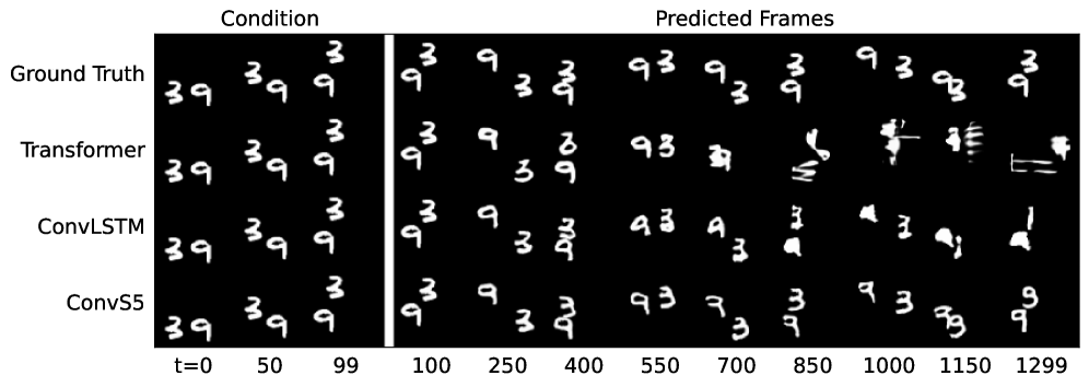
(a) Example 1

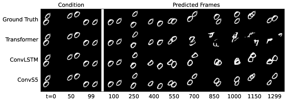
(b) Example 2

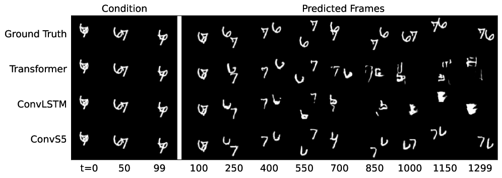
(c) Example 3

Figure 3: Moving-MNIST Samples: 1200 frames generated conditioned on 100.

C.2 3D Environments

Table 8: Full results for DMLab long-range benchmark dataset [13]. Results from Yan et al. [13] are indicated with $*$. We separate out the methods trained using the TECO [13] training framework in the bottom of the table. TECO-ConvSSM (ablation) refers to the ablation performed by randomly initializing the state kernel (see Section 5.3 and Appendix D.5).

	DMLab
Method	Params	FVD $\downarrow$	PSNR $\uparrow$	SSIM $\uparrow$	LPIPS $\downarrow$
FitVid*	165M	$176\pm 4.86$	$12.0\pm 0.013$	$0.356\pm 0.00171$	$0.491\pm 0.00108$
CW-VAE*	111M	$125\pm 7.95$	$12.6\pm 0.059$	$0.372\pm 0.00033$	$0.465\pm 0.00156$
Perceiver AR  *	30M	$96.3\pm 3.64$	$11.2\pm 0.004$	$0.304\pm 0.00004$	$0.487\pm 0.00123$
Latent FDM*	31M	$181\pm 2.20$	$17.8\pm 0.111$	$0.588\pm 0.00453$	$0.222\pm 0.00493$
Transformer	152M	$97.0\pm 5.98$	$\underline{19.9\pm 0.108}$	$0.619\pm 0.00506$	$\underline{0.123\pm 0.00191}$
Performer	152M	$\underline{80.3\pm 3.21}$	$17.3\pm 0.074$	$0.513\pm 0.00492$	$0.205\pm 0.00315$
S5	140M	$221\pm 13.1$	$19.3\pm 0.128$	$\underline{0.641\pm 0.00400}$	$0.162\pm 0.04510$
ConvS5	100M	$\mathbf{66.6\pm 4.81}$	$\mathbf{23.2\pm 0.053}$	$\mathbf{0.769\pm 0.01020}$	$\mathbf{0.079\pm 0.00073}$
TECO-Transformer*	173M	$\mathbf{27.5\pm 1.77}$	$\underline{22.4\pm 0.368}$	$\underline{0.709\pm 0.0119}$	$0.155\pm 0.00958$
TECO-Transformer (our run)	173M	$\mathbf{28.2\pm 0.66}$	$21.6\pm 0.079$	$0.696\pm 0.02640$	$\mathbf{0.082\pm 0.00119}$
TECO-S5	180M	$34.6\pm 0.26$	$20.1\pm 0.037$	$0.687\pm 0.00132$	$0.143\pm 0.00049$
TECO-ConvSSM (ablation)	175M	$44.3\pm 2.69$	$21.0\pm 0.106$	$0.691\pm 0.00004$	$0.010\pm 0.00267$
TECO-ConvS5	175M	$\underline{31.2\pm 0.23}$	$\mathbf{23.8\pm 0.056}$	$\mathbf{0.803\pm 0.0020}$	$\underline{0.085\pm 0.00179}$

Table 9: Full results for ablation of ConvS5 convolutional ablations for DMLab long-range benchmark dataset [13]. To make parameter counts comparable for different configurations, when possible, we adjust parameters in the activation blocks, e.g. increasing the size of the ResNet convolution kernels or increasing the features of the GLU activation. With these adjustments, the models also have similar training speeds. Note the last entry is the S5 run which serves as an additional ablation of the convolutional structure.

	DMLab
$\mathbfcal{B}$ kernel	$\mathbfcal{C}$ kernel	Activation	Params	FVD $\downarrow$	PSNR $\uparrow$	SSIM $\uparrow$	LPIPS $\downarrow$	Train Step Time (s) $\downarrow$
$3\times 3$	$3\times 3$	ResNet	100M	$\mathbf{66.6\pm 4.81}$	$\mathbf{23.2\pm 0.053}$	$\mathbf{0.769\pm 0.00043}$	$\mathbf{0.079\pm 0.00073}$	2.31
$1\times 1$	$3\times 3$	ResNet	85M	$67.5\pm 0.73$	$22.8\pm 0.041$	$0.756\pm 0.00039$	$0.085\pm 0.00124$	2.52
$1\times 1$	$1\times 1$	ResNet	100M	$81.1\pm 6.06$	$23.0\pm 0.074$	$0.767\pm 0.00186$	$0.083\pm 0.00139$	$2.21$
$3\times 3$	$3\times 3$	GLU	71M	$96.1\pm 5.20$	$22.7\pm 0.157$	$0.762\pm 0.00363$	$0.088\pm 0.00287$	2.75
$1\times 1$	$5\times 5$	GLU	83M	$89.1\pm 0.61$	$21.5\pm 0.072$	$0.713\pm 0.00290$	$0.106\pm 0.00289$	2.58
$1\times 1$	$1\times 1$	GLU	30M	$187\pm 2.77$	$21.0\pm 0.064$	$0.689\pm 0.00007$	$0.112\pm 0.00183$	$1.73$
-	-	GLU	140M	$221\pm 13.1$	$19.3\pm 0.128$	$0.641\pm 0.00400$	$0.162\pm 0.04510$	1.34

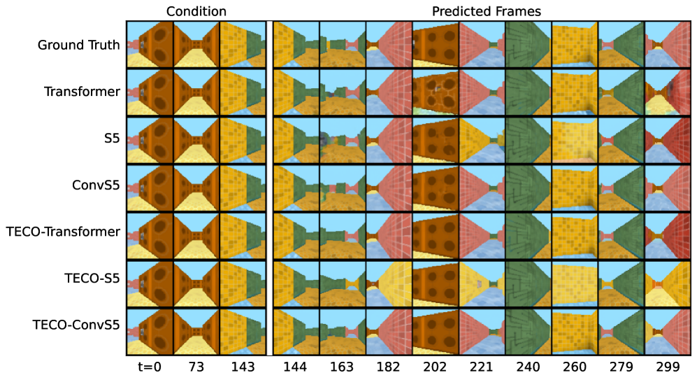
(a) 156 frames generated conditioned on 144 (action-conditioned).

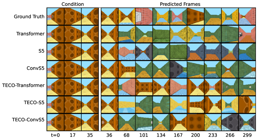
(b) 264 frames generated conditioned on 36 (no action-conditioning).

Figure 4: DMLab Samples

Table 10: Full results on the Minecraft and Habitat long-range benchmark datasets [13]. Results from Yan et al. [13] are indicated with $*$. Note that Yan et al. [13] did not evaluate FitVid or CW-VAE on Habitat due to cost.

Minecraft Method Params FVD $\downarrow$ PSNR $\uparrow$ SSIM $\uparrow$ LPIPS $\downarrow$ FitVid* 176M $956\pm 15.8$ $13.0\pm 0.0089$ $0.343\pm 0.00380$ $0.519\pm 0.00367$ CW-VAE* 140M $397\pm 15.5$ $13.4\pm 0.0610$ $0.338\pm 0.00274$ $0.441\pm 0.00367$ Perceiver AR* 166M $\underline{76.3\pm 1.72}$ $13.2\pm 0.0711$ $0.323\pm 0.00336$ $0.441\pm 0.00207$ Latent FDM* 33M $167\pm 6.26$ $13.4\pm 0.0904$ $0.349\pm 0.00327$ $0.429\pm 0.00284$ TECO-Transformer* 274M $116\pm 5.08$ $\mathbf{15.4\pm 0.0603}$ $\mathbf{0.381\pm 0.00192}$ $\mathbf{0.340\pm 0.00264}$ TECO-ConvS5 214M $\mathbf{70.7\pm 3.05}$ $\underline{14.8\pm 0.0984}$ $\underline{0.374\pm 0.00414}$ $\underline{0.355\pm 0.00467}$ Habitat Method Params FVD $\downarrow$ PSNR $\uparrow$ SSIM $\uparrow$ LPIPS $\downarrow$ Perceiver AR* 200M $164\pm 12.6$ $\underline{12.8\pm 0.0423}$ $\mathbf{0.405\pm 0.00248}$ $0.676\pm 0.00282$ Latent FDM* 87M $433\pm 2.67$ $12.5\pm 0.0121$ $0.311\pm 0.00083$ $\mathbf{0.582\pm 0.00049}$ TECO-Transformer* 386M $\mathbf{76.3\pm 1.72}$ $\underline{12.8\pm 0.0139}$ $0.363\pm 0.00122$ $\underline{0.604\pm 0.00451}$ TECO-ConvS5 351M $\underline{95.1\pm 3.74}$ $\mathbf{12.9\pm 0.212}$ $\underline{0.390\pm 0.01238}$ $0.632\pm 0.00823$

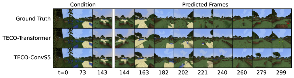
(a) 156 frames generated conditioned on 144 (action-conditioned).

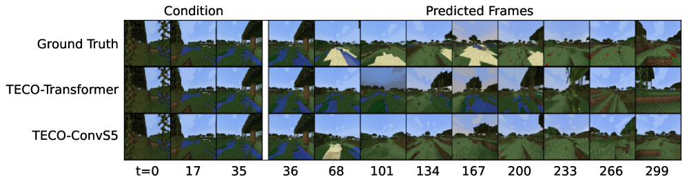
(b) 264 frames generated conditioned on 36 (action-conditioned).

Figure 5: Minecraft Samples

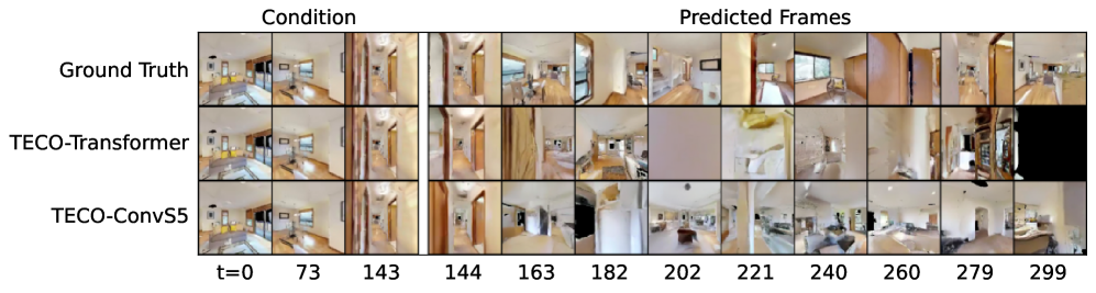
(a) 156 frames generated conditioned on 144 (action-conditioned).

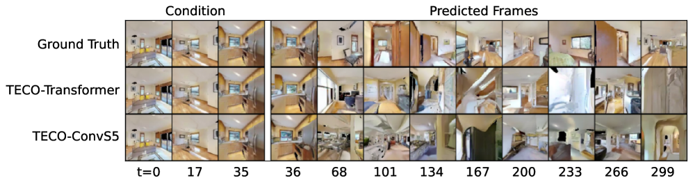
(b) 264 frames generated conditioned on 36 (no action-conditioning).

Figure 6: Habitat Samples

Table 11: Model runtime comparison for 3D Environment results in Tables 8-10. The implementations of the baselines FitVid, CW-VAE, Perceiver AR and Latent FDM used in the TECO work [13] are not publicly available in the TECO repository, so we were unable to include direct runtime comparisons for those methods.

DMLab Method Train Step Time (s) $\downarrow$ Sampling Speed (frames/s) Transformer $\mathbf{1.25\ (1.0\times)}$ $9.1\ (1.0\times)$ Performer $\underline{1.25\ (1.0\times)}$ $7.6(0.8\times)$ S5 $1.34\ (1.1\times)$ $\underline{28\ (3.1\times)}$ ConvS5 $2.31\ (1.8\times)$ $\mathbf{56\ (6.2\times)}$ TECO-Transformer $\mathbf{0.75\ (0.6\times)}$ $16\ (1.8\times)$ TECO-S5 $\underline{0.81\ (0.7\times)}$ $\mathbf{21\ (2.3\times)}$ TECO-ConvS5 $1.17\ (0.9\times)$ $\underline{18\ (2.0\times)}$ Minecraft Method Train Step Time (s) $\downarrow$ Sampling Speed (frames/s) TECO-Transformer $\mathbf{1.91\ (1.0\times)}$ $\underline{8.1\ (1.0\times)}$ TECO-ConvS5 $\underline{2.53\ (1.3\times)}$ $\mathbf{14\ (1.7\times)}$ Habitat Method Train Step Time (s) $\downarrow$ Sampling Speed (frames/s) TECO-Transformer $\mathbf{2.71\ (1.0\times)}$ $\underline{6.8\ (1.0\times)}$ TECO-ConvS5 $\underline{3.10\ (1.1\times)}$ $\mathbf{11\ (1.6\times)}$

Appendix D Experiment Configurations

Our codebase modifies the TECO codebase from Yan et al. [13] and we reuse their core Transformer and TECO framework implementations. More architectural details and dataset-specific details are described below.

D.1 Spatiotemporal Sequence Model Architectures

ConvS5, ConvLSTM and S5 models are formed by stacking multiple ConvS5, ConvLSTM or S5 layers, respectively. For each of these models, layer normalization [107] with a post-norm setup is used along with residual connections. For the Transformer, we use the Transformer implementation from Yan et al. [13] which consists of a stack of multi-head attention layers.

ConvS5 and ConvLSTM are applied directly to sequences of frames of shape [sequence length, latent height, latent width, latent features], where the original data has been convolved to a latent resolution and latent number of features. Since S5 and Transformer act on vector-valued sequences, these models require an additional downsampling convolution operation to project the latent frames into a token and an upsampling transposed convolution operation to project the Transformer backbone output tokens back into latent frames. We use the same sequence of compression operations for this as in Yan et al. [13]. The Encoder and Decoder referred to for all models in the hyperparameter tables below consist of ResNet Blocks with $3\times 3$ kernels as implemented in Yan et al. [13].

D.2 Evaluation Metrics

We follow Yan et al. [13] and evaluate methods by computing Fréchet Video Distance (FVD) [108], peak signal-to-noise ratio (PSNR), structural similarity index measure [109] and Learned Perceptual Image Patch Similarity (LPIPS) [110] between sampled trajectories and ground truth trajectories. See Yan et al. [13] for a more in-depth discussion of the use of these metrics for the 3D environment benchmarks.

D.3 Compute

All models were trained with 32GB NVIDIA V100 GPUs. For Moving-MNIST, models were trained with 8 V100s. For all other experiments, models were trained with 16 V100s. We list V100 days in the hyperparameters, which denotes the number of days it would take to train on a single V100.

D.4 Moving-MNIST

All models were trained to minimize L1+L2 loss over the frames directly in pixel space, as in Su et al. [84]. We trained models on 300 frames. We then repeated the experiment and trained models on 600 frames. For ConvS5 and ConvLSTM, we fixed the hidden dimensions (layer input/output features) and state sizes to be 256, and we swept over the following learning rates [$1\times 10^{-4}$, $5\times 10^{-4}$, $1\times 10^{-3}$] and chose the best model. For Transformer, we swept over model size, considering hidden dimensions of [512, 2014] and learning rates [$1\times 10^{-4}$, $5\times 10^{-4}$, $1\times 10^{-3}$] and chose the best model. We also observed better performance for the Transformer by convolving frames down to an $8\times 8$ latent resolution (rather than the $16\times 16$ used by ConvS5 and ConvLSTM) before downsampling to a token. All other relevant training parameters were kept the same between the three methods. See Tables 12-14 for detailed experiment configurations.

Each model was evaluated by collecting 1024 trajectories using the following procedure: condition on 100 frames from the ground truth test set, then generate forward 1200 frames. These samples were compared with the ground truth to compute FVD, PSNR, SSIM and LPIPS.

The ConvSSM ablation was performed using the exact settings as ConvS5, except the state kernel was initialized with a Gaussian and we swept over the following learning rates [$1\times 10^{-4}$, $5\times 10^{-4}$, $1\times 10^{-3}$].

Table 12: Experiment Configuration for ConvS5 on Moving-MNIST experiments

Hyperparameters		Moving-MNIST-300	Moving-MNIST-600
	V100 Days	25	50
	Params	20M	20M
	Input Resolution	$64\times 64$	$64\times 64$
	Latent Resolution	$16\times 16$	$16\times 16$
	Batch Size	8	8
	Sequence Length	300	600
	LR	$1\times 10^{-3}$	$1\times 10^{-3}$
	LR Schedule	cosine	cosine
	Warmup Steps	5k	5k
	Max Training Steps	300K	300K
	Weight Decay	$1\times 10^{-5}$	$1\times 10^{-5}$
Encoder	Depths	64, 128, 256	64, 128, 256
	Blocks	1	1
Decoder	Depths	64, 128, 256	64, 128, 256
	Blocks	1	1
ConvS5	Hidden Dim ($U$)	256	256
	State Size ($P$)	256	256
	$\mathbfcal{B}$ Kernel Size	$3\times 3$	$3\times 3$
	$\mathbfcal{C}$ Kernel Size	$3\times 3$	$3\times 3$
	Layers	8	8
	Dropout	0	0
	Activation	ResNet	ResNet

Table 13: Experiment Configuration for ConvLSTM on Moving-MNIST experiments

Hyperparameters		Moving-MNIST-300	Moving-MNIST-600
	V100 Days	75	150
	Params	20M	20M
	Input Resolution	$64\times 64$	$64\times 64$
	Latent Resolution	$16\times 16$	$16\times 16$
	Batch Size	8	8
	Sequence Length	300	600
	LR	$5\times 10^{-4}$	$5\times 10^{-4}$
	LR Schedule	cosine	cosine
	Warmup Steps	5k	5k
	Max Training Steps	300K	300K
	Weight Decay	$1\times 10^{-5}$	$1\times 10^{-5}$
Encoder	Depths	64, 128, 256	64, 128, 256
	Blocks	1	1
Decoder	Depths	64, 128, 256	64, 128, 256
	Blocks	1	1
ConvLSTM	Hidden Dim	256	256
	State Size	256	256
	Kernel Size	$3\times 3$	$3\times 3$
	Layers	8	8
	Dropout	0	0

Table 14: Experiment Configuration for Transformer on Moving-MNIST experiments

Hyperparameters		Moving-MNIST-300	Moving-MNIST-600
	V100 Days	25	50
	Params	164M	164M
	Input Resolution	$64\times 64$	$64\times 64$
	Latent Resolution	$8\times 8$	$8\times 8$
	Batch Size	8	8
	Sequence Length	300	600
	LR	$5\times 10^{-4}$	$1\times 10^{-4}$
	LR Schedule	cosine	cosine
	Warmup Steps	5k	5k
	Max Training Steps	300K	300K
	Weight Decay	$1\times 10^{-5}$	$1\times 10^{-5}$
Encoder	Depths	64, 128, 256, 512	64, 128, 256, 512
	Blocks	1	1
Decoder	Depths	64, 128, 256, 512	64, 128, 256, 512
	Blocks	1	1
Temporal Transformer	Downsample Factor	8	8
	Hidden Dim	1024	1024
	Feedforward Dim	4096	4096
	Heads	16	16
	Layers	8	8
	Dropout	0	0

D.5 Long-Range 3D Environment Benchmarks

We follow the procedures from Yan et al. [13] and train models on the same pre-trained vector-quantized (VQ) $16\times 16$ codes used by the baselines evaluated in that work. Models were trained to optimize a cross-entropy reconstruction loss between the predictions and true VQ codes. The evaluation of DMLab and Habitat involves both an action-conditioned and unconditioned setting. Therefore, as in Yan et al. [13], the actions were randomly dropped out half the time during training on these datasets.

After training, we follow the procedure from Yan et al. [13] for evaluation in two different settings. The first setting involves computing PSNR, SSIM and LPIPS from 1024 samples generated by conditioning on the first 144 frames and then generating the next 156 frames while providing the model with past and future actions. The second setting does not provide actions as input (with the exception of Minecraft, which also provides actions in this setting). It involves computing FVD using 1024 samples generated by conditioning on the first 36 frames and then predicting the remaining 264 frames.

All sequence models we trained used the same number of layers as the Transformer used in the TECO-Transformer trained by Yan et al. [13]. In addition, the TECO-Transformer, TECO-S5 and TECO-ConvS5 models we trained used the exact encoder/decoder configuration and MaskGit configuration as in Yan et al. [13]. The Transformer, S5 and ConvS5 models we trained without the TECO framework were all trained using the same encoder/decoder configuration. See Tables 15-21 for more detailed experimental configuration details. See dataset-specific paragraphs below for hyperparameter tuning information.

TECO Training Framework

Yan et al. [13] proposed the TECO training framework to train Transformers on long video data. For some of our experiments, we use ConvS5 layers and S5 layers as a drop-in replacement for the Transformer in this framework. We refer the reader to Yan et al. [13] for full details. Briefly, given the original VQ codes, TECO trains an additional encoder/decoder that compresses the frames to a lower latent resolution (e.g., from $16\times 16$ to $8\times 8$ ) by training an additional encoder/decoder with a codebook loss, $\mathcal{L}_{\mathrm{VQ}}$. In addition, a MaskGit [98] dynamics prior loss, $\mathcal{L}_{\mathrm{prior}}$, is used for the latent transitions. The sequence model (e.g. Transformer, S5, ConvS5) takes the latent frames (compressed into tokens in the case of Transformer and S5) and produces an output which is used along with the latents by the decoder to produce predictions and a reconstruction loss, $\mathcal{L}_{\mathrm{recon}}$. Models are trained to minimize the following total loss:

$$\mathcal{L}_{\mathrm{TECO}} =\mathcal{L}_{\mathrm{VQ}}+\mathcal{L}_{\mathrm{recon}}+\mathcal{L}_{\mathrm{prior}}.$$ (32)

In addition, TECO includes the use of DropLoss [13], which drops out a percentage of random timesteps that are not decoded and therefore do not require computing the expensive $\mathcal{L}_{\mathrm{recon}}$ and $\mathcal{L}_{\mathrm{prior}}$ terms.

DMLab

As mentioned above, the actions were randomly dropped out of sequences half the time (due to the two evaluation scenarios, action-conditioned and unconditioned). We observed that for DMLab, when provided past and future actions, models converged faster using the simple masking strategy discussed in Gu et al. [19] that masks the future inputs rather than feeding the predicted inputs (or true inputs during training) autoregressively. Therefore we trained all models (Transformer, Performer, S5, ConvS5, Teco-Transformer, TECO-S5, TECO-ConvS5) by using this strategy when the actions were provided, and using the autoregressive strategy when actions were not provided. We observed this significantly improved the LPIPS of the Transformer baselines. Note, in pilot runs for Minecraft and Habitat, we observed this strategy led to lower-quality frames and did not use it for the reported results for those datasets.

We trained each model, Transformer, Performer, S5, ConvS5, Teco-Transformer, TECO-S5, TECO-ConvS5, with three different learning rates [$1\times 10^{-4}$, $5\times 10^{-4}$, $1\times 10^{-3}$] and selected the best run for each model. See Tables 15-20 for more experiment configuration details.

The TECO-ConvSSM ablation used the exact same settings as TECO-ConvS5, except the state kernel was initialized with a random Gaussian and a lower learning rate of $1\times 10^{-5}$ was required for stable training.

Table 15: Experiment Configuration for ConvS5 on DMLab

Hyperparameters		DMLab
	V100 Days	150
	Params	101M
	Input Resolution	$64\times 64$
	Latent Resolution	$16\times 16$
	Batch Size	16
	Sequence Length	300
	LR	$5\times 10^{-4}$
	LR Schedule	cosine
	Warmup Steps	5k
	Max Training Steps	500K
	Weight Decay	$1\times 10^{-5}$
Encoder	Depths	256
	Blocks	1
Decoder	Depths	256
	Blocks	4
ConvS5	Hidden Dim ($U$)	512
	State Size ($P$)	512
	$\mathbfcal{B}$ Kernel Size	$3\times 3$
	$\mathbfcal{C}$ Kernel Size	$3\times 3$
	Layers	8
	Dropout	0
	Activation	ResNet

Table 16: Experiment Configuration for S5 on DMLab

Hyperparameters		DMLab
	V100 Days	125
	Params	140M
	Input Resolution	$64\times 64$
	Latent Resolution	$16\times 16$
	Batch Size	16
	Sequence Length	300
	LR	$1\times 10^{-3}$
	LR Schedule	cosine
	Warmup Steps	5k
	Max Training Steps	500K
	Weight Decay	$1\times 10^{-5}$
Encoder	Depths	256
	Blocks	1
Decoder	Depths	256
	Blocks	4
S5	Downsample Factor	16
	Hidden Dim ($U$)	1024
	State Size ($P$)	1024
	Layers	8
	Dropout	0
	Activation	GLU (half)

Table 17: Experiment Configuration for Transformer on DMLab

Hyperparameters		DMLab
	V100 Days	125
	Params	152M
	Input Resolution	$64\times 64$
	Latent Resolution	$16\times 16$
	Batch Size	16
	Sequence Length	300
	LR	$5\times 10^{-4}$
	LR Schedule	cosine
	Warmup Steps	5k
	Max Training Steps	500K
	Weight Decay	$1\times 10^{-5}$
Encoder	Depths	256
	Blocks	1
Decoder	Depths	256
	Blocks	4
Temporal Transformer	Downsample Factor	16
	Hidden Dim	512
	Feedforward Dim	2048
	Heads	16
	Layers	8
	Dropout	0

Table 18: Experiment Configuration for TECO-ConvS5 on DMLab

Hyperparameters	DMLab
	V100 Days	110
	Params	175M
	Input Resolution	$64\times 64$
	Latent Resolution	$8\times 8$
	Batch Size	16
	Sequence Length	300
	LR	$5\times 10^{-4}$
	LR Schedule	cosine
	Warmup Steps	5k
	Max Training Steps	500K
	Weight Decay	$1\times 10^{-5}$
	DropLoss Rate	0.9
Encoder	Depths	256, 512
	Blocks	2
Codebook	Size	1024
	Embedding Dim	32
Decoder	Depths	256, 512
	Blocks	4
ConvS5	Hidden Dim ($U$)	512
	State Size ($P$)	1024
	$\mathbfcal{B}$ Kernel Size	$3\times 3$
	$\mathbfcal{C}$ Kernel Size	$3\times 3$
	Layers	8
	Dropout	0
	Activation	ResNet
MaskGit	Mask Schedule	cosine
	Hidden Dim	512
	Feedforward Dim	2048
	Heads	8
	Layers	8
	Dropout	0

Table 19: Experiment Configuration for TECO-S5 on DMLab

Hyperparameters	DMLab
	V100 Days	80
	Params	180M
	Input Resolution	$64\times 64$
	Latent Resolution	$8\times 8$
	Batch Size	16
	Sequence Length	300
	LR	$1\times 10^{-3}$
	LR Schedule	cosine
	Warmup Steps	5k
	Max Training Steps	500K
	Weight Decay	$1\times 10^{-5}$
	DropLoss Rate	0.9
Encoder	Depths	256, 512
	Blocks	2
Codebook	Size	1024
	Embedding Dim	32
Decoder	Depths	256, 512
	Blocks	4
S5	Downsample Factor	8
	Hidden Dim ($U$)	2048
	State Size ($P$)	2048
	Layers	8
	Dropout	0
	Activation	GLU (half)
MaskGit	Mask Schedule	cosine
	Hidden Dim	512
	Feedforward Dim	2048
	Heads	8
	Layers	8
	Dropout	0

Table 20: Experiment Configuration for TECO-Transformer on DMLab

Hyperparameters	DMLab
	V100 Days	80
	Params	173M
	Input Resolution	$64\times 64$
	Latent Resolution	$8\times 8$
	Batch Size	16
	Sequence Length	300
	LR	$1\times 10^{-4}$
	LR Schedule	cosine
	Warmup Steps	5k
	Max Training Steps	500K
	Weight Decay	$1\times 10^{-5}$
	DropLoss Rate	0.9
Encoder	Depths	256, 512
	Blocks	2
Codebook	Size	1024
	Embedding Dim	32
Decoder	Depths	256, 512
	Blocks	4
Temporal Transformer	Downsample Factor	8
	Hidden Dim	1024
	Feedforward Dim	4096
	Heads	16
	Layers	8
	Dropout	0
MaskGit	Mask Schedule	cosine
	Hidden Dim	512
	Feedforward Dim	2048
	Heads	8
	Layers	8
	Dropout	0

Minecraft and Habitat

For Minecraft and Habitat, we only trained TECO-ConvS5 due to the costs of training on these datasets. See dataset details in Appendix E and reported compute costs in Yan et al. [13]. For Minecraft, we evaluated two different learning rates [$1\times 10^{-4}$, $5\times 10^{-4}$] and chose the best. For Habitat, we only performed one run with no further tuning. See Table 21 for further experiment configuration details.

Table 21: Experiment Configuration for TECO-ConvS5 on Minecraft and Habitat

Hyperparameters		Minecraft	Habitat
	V100 Days	470	575
	Params	214M	351M
	Input Resolution	$128\times 128$	$128\times 128$
	Latent Resolution	$8\times 8$	$8\times 8$
	Batch Size	16	16
	Sequence Length	300	300
	LR	$5\times 10^{-4}$	$1\times 10^{-4}$
	LR Schedule	cosine	cosine
	Warmup Steps	5k	5k
	Max Training Steps	1M	1M
	DropLoss Rate	0.9	0.9
Encoder	Depths	256, 512	256, 512
	Blocks	4	4
Codebook	Size	1024	1024
	Embedding Dim	32	32
Decoder	Depths	256, 512	256, 512
	Blocks	8	8
ConvS5	Hidden Dim ($U$)	512	512
	State Size ($P$)	512	512
	$\mathbfcal{B}$ Kernel Size	$3\times 3$	$3\times 3$
	$\mathbfcal{C}$ Kernel Size	$3\times 3$	$3\times 3$
	Layers	12	8
	Dropout	0	0
	Activation	ResNet	ResNet
MaskGit	Mask Schedule	cosine	cosine
	Hidden Dim	768	1024
	Feedforward Dim	3072	4096
	Heads	12	16
	Layers	6	16
	Dropout	0	0

Appendix E Datasets

E.1 Moving-MNIST

The Moving-MNIST [54] dataset is generated by moving two $28\times 28$ size MNIST digits from the MNIST dataset [111] inside a $64\times 64$ black background. The digits begin at a random initial location, and move with constant velocity, bouncing when they reach the boundary. For each of the sequence lengths we consider, 300 and 600, we follow Wang et al. [81] and Su et al. [84] and generate 10,000 sequences for training.

E.2 DMLab

We use the DMLab long-range benchmark designed by Yan et al. [13] using the DeepMind Lab (DMLab) [99] simulator. The simulator generates random 3D mazes with random floor and wall textures. The benchmark consists of 40K action-conditioned, 300 frame videos at a $64\times 64$ resolution. The videos are of an agent randomly navigating $7\times 7$ mazes by choosing random points in the maze and navigating to them through the shortest path.

E.3 Minecraft

We use the Minecraft [100] long-range benchmark designed by Yan et al. [13]. The game features 3D worlds that contain complex terrains such as hills, forests, rivers and lakes. The benchmark was constructed by collecting 200K action-conditioned 300 frame videos at a $128\times 128$ resolution. The videos are in Minecraft’s marsh biome and the agent iterates walking forward for a random number of steps and randomly rotating left or right. This results in parts of the scene going out of view and coming back into view later.

E.4 Habitat

We use the Habitat long-range benchmark designed by Yan et al. [13] using the Habitat simulator [101]. The simulator renders trajectories using scans of real 3D scenes. Yan et al. [13] compiled  1400 indoor scans from HM3D [112], Matterport3D [113] and Gibson [114] to generate 200K action-conditioned, 300 frame videos with a $128\times 128$ resolution. Yan et al. [13] used Habitat’s in-built path traversal algorithm to construct action trajectories that move the agent between randomly sampled locations.

References

- Finn et al. [2016] Chelsea Finn, Ian Goodfellow, and Sergey Levine. Unsupervised learning for physical interaction through video prediction. Advances in neural information processing systems, 29, 2016.
- Xu et al. [2019] Yi Xu, Longwen Gao, Kai Tian, Shuigeng Zhou, and Huyang Sun. Non-local ConvLSTM for video compression artifact reduction. In Proceedings of the IEEE/CVF international conference on computer vision, pages 7043–7052, 2019.
- Huang et al. [2021] He Huang, Zheni Zeng, Danya Yao, Xin Pei, and Yi Zhang. Spatial-temporal ConvLSTM for vehicle driving intention prediction. Tsinghua Science and Technology, 27(3):599–609, 2021.
- Chen et al. [2020] Xiaoyu Chen, Xingsheng Xie, and Da Teng. Short-term traffic flow prediction based on ConvLSTM model. In 2020 IEEE 5th Information Technology and Mechatronics Engineering Conference (ITOEC), pages 846–850. IEEE, 2020.
- Pathak et al. [2022] Jaideep Pathak, Shashank Subramanian, Peter Harrington, Sanjeev Raja, Ashesh Chattopadhyay, Morteza Mardani, Thorsten Kurth, David Hall, Zongyi Li, Kamyar Azizzadenesheli, et al. Fourcastnet: A global data-driven high-resolution weather model using adaptive Fourier neural operators. arXiv preprint arXiv:2202.11214, 2022.
- Weyn et al. [2021] Jonathan A Weyn, Dale R Durran, Rich Caruana, and Nathaniel Cresswell-Clay. Sub-seasonal forecasting with a large ensemble of deep-learning weather prediction models. Journal of Advances in Modeling Earth Systems, 13(7):e2021MS002502, 2021.
- Ho et al. [2022] Jonathan Ho, Tim Salimans, Alexey A. Gritsenko, William Chan, Mohammad Norouzi, and David J. Fleet. Video diffusion models. In Alice H. Oh, Alekh Agarwal, Danielle Belgrave, and Kyunghyun Cho, editors, Advances in Neural Information Processing Systems, 2022.
- Clark et al. [2019] Aidan Clark, Jeff Donahue, and Karen Simonyan. Adversarial video generation on complex datasets. arXiv preprint arXiv:1907.06571, 2019.
- Yan et al. [2021] Wilson Yan, Yunzhi Zhang, Pieter Abbeel, and Aravind Srinivas. Videogpt: Video generation using VQ-VAE and Transformers. arXiv preprint arXiv:2104.10157, 2021.
- Le Moing et al. [2021] Guillaume Le Moing, Jean Ponce, and Cordelia Schmid. CCVS: context-aware controllable video synthesis. Advances in Neural Information Processing Systems, 34:14042–14055, 2021.
- Tian et al. [2021] Yu Tian, Jian Ren, Menglei Chai, Kyle Olszewski, Xi Peng, Dimitris N. Metaxas, and Sergey Tulyakov. A good image generator is what you need for high-resolution video synthesis. In International Conference on Learning Representations, 2021.
- Luc et al. [2020] Pauline Luc, Aidan Clark, Sander Dieleman, Diego de Las Casas, Yotam Doron, Albin Cassirer, and Karen Simonyan. Transformation-based adversarial video prediction on large-scale data. arXiv preprint arXiv:2003.04035, 2020.
- Yan et al. [2022] Wilson Yan, Danijar Hafner, Stephen James, and Pieter Abbeel. Temporally consistent video Transformer for long-term video prediction. arXiv preprint arXiv:2210.02396, 2022.
- Ge et al. [2022] Songwei Ge, Thomas Hayes, Harry Yang, Xi Yin, Guan Pang, David Jacobs, Jia-Bin Huang, and Devi Parikh. Long video generation with time-agnostic VQGAN and time-sensitive Transformer. In Computer Vision–ECCV 2022: 17th European Conference, Tel Aviv, Israel, October 23–27, 2022, Proceedings, Part XVII, pages 102–118. Springer, 2022.
- Harvey et al. [2022] William Harvey, Saeid Naderiparizi, Vaden Masrani, Christian Dietrich Weilbach, and Frank Wood. Flexible diffusion modeling of long videos. In Alice H. Oh, Alekh Agarwal, Danielle Belgrave, and Kyunghyun Cho, editors, Advances in Neural Information Processing Systems, 2022.
- Saxena et al. [2021] Vaibhav Saxena, Jimmy Ba, and Danijar Hafner. Clockwork variational autoencoders. Advances in Neural Information Processing Systems, 34:29246–29257, 2021.
- Shi et al. [2015] Xingjian Shi, Zhourong Chen, Hao Wang, Dit-Yan Yeung, Wai-Kin Wong, and Wang-chun Woo. Convolutional LSTM network: A machine learning approach for precipitation nowcasting. Advances in neural information processing systems, 28, 2015.
- Ballas et al. [2015] Nicolas Ballas, Li Yao, Chris Pal, and Aaron Courville. Delving deeper into convolutional networks for learning video representations. arXiv preprint arXiv:1511.06432, 2015.
- Gu et al. [2021a] Albert Gu, Karan Goel, and Christopher Re. Efficiently modeling long sequences with structured state spaces. In International Conference on Learning Representations, 2021a.
- Smith et al. [2023] Jimmy T.H. Smith, Andrew Warrington, and Scott Linderman. Simplified state space layers for sequence modeling. In The Eleventh International Conference on Learning Representations, 2023.
- Hochreiter and Schmidhuber [1997] Sepp Hochreiter and Jürgen Schmidhuber. Long short-term memory. Neural Computation, 9(8):1735–1780, 1997.
- Cho et al. [2014] Kyunghyun Cho, Bart Van Merriënboer, Caglar Gulcehre, Dzmitry Bahdanau, Fethi Bougares, Holger Schwenk, and Yoshua Bengio. Learning phrase representations using rnn encoder-decoder for statistical machine translation. arXiv preprint arXiv:1406.1078, 2014.
- Pascanu et al. [2013] Razvan Pascanu, Tomas Mikolov, and Yoshua Bengio. On the difficulty of training recurrent neural networks. In International Conference on Machine Learning, pages 1310–1318. PMLR, 2013.
- Vaswani et al. [2017] Ashish Vaswani, Noam Shazeer, Niki Parmar, Jakob Uszkoreit, Llion Jones, Aidan N Gomez, Łukasz Kaiser, and Illia Polosukhin. Attention is all you need. Advances in Neural Information Processing Systems, 30, 2017.
- Dosovitskiy et al. [2021] Alexey Dosovitskiy, Lucas Beyer, Alexander Kolesnikov, Dirk Weissenborn, Xiaohua Zhai, Thomas Unterthiner, Mostafa Dehghani, Matthias Minderer, Georg Heigold, Sylvain Gelly, Jakob Uszkoreit, and Neil Houlsby. An image is worth 16x16 words: Transformers for image recognition at scale. In International Conference on Learning Representations, 2021.
- Arnab et al. [2021] Anurag Arnab, Mostafa Dehghani, Georg Heigold, Chen Sun, Mario Lučić, and Cordelia Schmid. ViViT: A video vision Transformer. In Proceedings of the IEEE/CVF international conference on computer vision, pages 6836–6846, 2021.
- Gupta et al. [2022a] Agrim Gupta, Stephen Tian, Yunzhi Zhang, Jiajun Wu, Roberto Martín-Martín, and Li Fei-Fei. Maskvit: Masked visual pre-training for video prediction. arXiv preprint arXiv:2206.11894, 2022a.
- Van Den Oord et al. [2017] Aaron Van Den Oord, Oriol Vinyals, et al. Neural discrete representation learning. Advances in neural information processing systems, 30, 2017.
- Walker et al. [2021] Jacob Walker, Ali Razavi, and Aäron van den Oord. Predicting video with VQVAE. arXiv preprint arXiv:2103.01950, 2021.
- Esser et al. [2021] Patrick Esser, Robin Rombach, and Bjorn Ommer. Taming Transformers for high-resolution image synthesis. In Proceedings of the IEEE/CVF conference on computer vision and pattern recognition, pages 12873–12883, 2021.
- Pope et al. [2022] Reiner Pope, Sholto Douglas, Aakanksha Chowdhery, Jacob Devlin, James Bradbury, Anselm Levskaya, Jonathan Heek, Kefan Xiao, Shivani Agrawal, and Jeff Dean. Efficiently scaling Transformer inference. arXiv preprint arXiv:2211.05102, 2022.
- Dao et al. [2022] Tri Dao, Dan Fu, Stefano Ermon, Atri Rudra, and Christopher Ré. FlashAttention: Fast and memory-efficient exact attention with IO-awareness. Advances in Neural Information Processing Systems, 35:16344–16359, 2022.
- Choromanski et al. [2021] Krzysztof Marcin Choromanski, Valerii Likhosherstov, David Dohan, Xingyou Song, Andreea Gane, Tamas Sarlos, Peter Hawkins, Jared Quincy Davis, Afroz Mohiuddin, Lukasz Kaiser, David Benjamin Belanger, Lucy Colwell, and Adrian Weller. Rethinking attention with Performers. In International Conference on Learning Representations, 2021.
- Katharopoulos et al. [2020] Angelos Katharopoulos, Apoorv Vyas, Nikolaos Pappas, and François Fleuret. Transformers are RNNs: Fast autoregressive Transformers with linear attention. In International Conference on Machine Learning, pages 5156–5165. PMLR, 2020.
- Kitaev et al. [2020] Nikita Kitaev, Lukasz Kaiser, and Anselm Levskaya. Reformer: The efficient Transformer. In International Conference on Learning Representations, 2020.
- Beltagy et al. [2020] Iz Beltagy, Matthew Peters, and Arman Cohan. Longformer: The long-document Transformer. arXiv preprint arXiv:2004.05150, 2020.
- Gupta and Berant [2020] Ankit Gupta and Jonathan Berant. Gmat: Global memory augmentation for Transformers, 2020.
- Wang et al. [2020a] Sinong Wang, Belinda Li, Madian Khabsa, Han Fang, and Hao Ma. Linformer: Self-attention with linear complexity. arXiv preprint arXiv:2006.04768, 2020a.
- Jaegle et al. [2021] Andrew Jaegle, Felix Gimeno, Andy Brock, Oriol Vinyals, Andrew Zisserman, and Joao Carreira. Perceiver: General perception with iterative attention. In International conference on machine learning, pages 4651–4664. PMLR, 2021.
- Tay et al. [2021] Yi Tay, Mostafa Dehghani, Samira Abnar, Yikang Shen, Dara Bahri, Philip Pham, Jinfeng Rao, Liu Yang, Sebastian Ruder, and Donald Metzler. Long Range Arena: A benchmark for efficient Transformers. In International Conference on Learning Representations, 2021.
- Gupta et al. [2022b] Ankit Gupta, Albert Gu, and Jonathan Berant. Diagonal state spaces are as effective as structured state spaces. In Advances in Neural Information Processing Systems, 2022b.
- Gu et al. [2022] Albert Gu, Karan Goel, Ankit Gupta, and Christopher Ré. On the parameterization and initialization of diagonal state space models. In Advances in Neural Information Processing Systems, 2022.
- Hasani et al. [2023] Ramin Hasani, Mathias Lechner, Tsun-Hsuan Wang, Makram Chahine, Alexander Amini, and Daniela Rus. Liquid structural state-space models. In International Conference on Learning Representations, 2023.
- Goel et al. [2022] Karan Goel, Albert Gu, Chris Donahue, and Christopher Re. It’s raw! Audio generation with state-space models. In Proceedings of the 39th International Conference on Machine Learning, volume 162 of Proceedings of Machine Learning Research, pages 7616–7633. PMLR, 17–23 Jul 2022.
- Nguyen et al. [2022] Eric Nguyen, Karan Goel, Albert Gu, Gordon Downs, Preey Shah, Tri Dao, Stephen Baccus, and Christopher Ré. S4ND: Modeling images and videos as multidimensional signals with state spaces. In Advances in Neural Information Processing Systems, 2022.
- Islam and Bertasius [2022] Md Mohaiminul Islam and Gedas Bertasius. Long movie clip classification with state-space video models. In Computer Vision–ECCV 2022: 17th European Conference, Tel Aviv, Israel, October 23–27, 2022, Proceedings, Part XXXV, pages 87–104, 2022.
- David et al. [2023] Shmuel Bar David, Itamar Zimerman, Eliya Nachmani, and Lior Wolf. Decision S4: Efficient sequence-based RL via state spaces layers. In The Eleventh International Conference on Learning Representations, 2023.
- Lu et al. [2023] Chris Lu, Yannick Schroecker, Albert Gu, Emilio Parisotto, Jakob Foerster, Satinder Singh, and Feryal Behbahani. Structured state space models for in-context reinforcement learning. arXiv preprint arXiv:2303.03982, 2023.
- Zhou et al. [2022] Linqi Zhou, Michael Poli, Winnie Xu, Stefano Massaroli, and Stefano Ermon. Deep latent state space models for time-series generation. arXiv preprint arXiv:2212.12749, 2022.
- Fu et al. [2023] Daniel Y Fu, Tri Dao, Khaled Kamal Saab, Armin W Thomas, Atri Rudra, and Christopher Re. Hungry hungry hippos: Towards language modeling with state space models. In The Eleventh International Conference on Learning Representations, 2023.
- Mehta et al. [2023] Harsh Mehta, Ankit Gupta, Ashok Cutkosky, and Behnam Neyshabur. Long range language modeling via gated state spaces. In The Eleventh International Conference on Learning Representations, 2023.
- Wang et al. [2022a] Junxiong Wang, Jing Nathan Yan, Albert Gu, and Alexander M Rush. Pretraining without attention. arXiv preprint arXiv:2212.10544, 2022a.
- Poli et al. [2023] Michael Poli, Stefano Massaroli, Eric Nguyen, Daniel Y Fu, Tri Dao, Stephen Baccus, Yoshua Bengio, Stefano Ermon, and Christopher Ré. Hyena hierarchy: Towards larger convolutional language models. arXiv preprint arXiv:2302.10866, 2023.
- Srivastava et al. [2015] Nitish Srivastava, Elman Mansimov, and Ruslan Salakhudinov. Unsupervised learning of video representations using LSTMs. In International conference on machine learning, pages 843–852. PMLR, 2015.
- Iserles [2009] Arieh Iserles. A first course in the numerical analysis of differential equations. 44. Cambridge university press, 2009.
- Gu et al. [2021b] Albert Gu, Isys Johnson, Karan Goel, Khaled Saab, Tri Dao, Atri Rudra, and Christopher Ré. Combining recurrent, convolutional, and continuous-time models with linear state space layers. Advances in Neural Information Processing Systems, 34, 2021b.
- Orvieto et al. [2023a] Antonio Orvieto, Samuel L Smith, Albert Gu, Anushan Fernando, Caglar Gulcehre, Razvan Pascanu, and Soham De. Resurrecting recurrent neural networks for long sequences. arXiv preprint arXiv:2303.06349, 2023a.
- Orvieto et al. [2023b] Antonio Orvieto, Soham De, Caglar Gulcehre, Razvan Pascanu, and Samuel L Smith. On the universality of linear recurrences followed by nonlinear projections. arXiv preprint arXiv:2307.11888, 2023b.
- Martin and Cundy [2018] Eric Martin and Chris Cundy. Parallelizing linear recurrent neural nets over sequence length. In International Conference on Learning Representations, 2018.
- Bradbury et al. [2017] James Bradbury, Stephen Merity, Caiming Xiong, and Richard Socher. Quasi-recurrent neural networks. In International Conference on Learning Representations, 2017.
- Lei et al. [2018] Tao Lei, Yu Zhang, Sida Wang, Hui Dai, and Yoav Artzi. Simple recurrent units for highly parallelizable recurrence. In Proceedings of the 2018 Conference on Empirical Methods in Natural Language Processing, pages 4470–4481, 2018.
- Gu et al. [2020] Albert Gu, Tri Dao, Stefano Ermon, Atri Rudra, and Christopher Ré. HiPPO: Recurrent memory with optimal polynomial projections. Advances in Neural Information Processing Systems, 33:1474–1487, 2020.
- Blelloch [1990] Guy Blelloch. Prefix sums and their applications. Technical report, Tech. rept. CMU-CS-90-190. School of Computer Science, Carnegie Mellon, 1990.
- Byeon et al. [2018] Wonmin Byeon, Qin Wang, Rupesh Kumar Srivastava, and Petros Koumoutsakos. ContextVP: Fully context-aware video prediction. In Proceedings of the European Conference on Computer Vision (ECCV), pages 753–769, 2018.
- Dumoulin and Visin [2016] Vincent Dumoulin and Francesco Visin. A guide to convolution arithmetic for deep learning. arXiv preprint arXiv:1603.07285, 2016.
- Chellapilla et al. [2006] Kumar Chellapilla, Sidd Puri, and Patrice Simard. High performance convolutional neural networks for document processing. In Tenth international workshop on frontiers in handwriting recognition. Suvisoft, 2006.
- Jia [2014] Yangqing Jia. Learning semantic image representations at a large scale. 2014.
- He et al. [2016] Kaiming He, Xiangyu Zhang, Shaoqing Ren, and Jian Sun. Deep residual learning for image recognition. In Proceedings of the IEEE conference on computer vision and pattern recognition, pages 770–778, 2016.
- Liu et al. [2022] Zhuang Liu, Hanzi Mao, Chao-Yuan Wu, Christoph Feichtenhofer, Trevor Darrell, and Saining Xie. A Convnet for the 2020s. In Proceedings of the IEEE/CVF Conference on Computer Vision and Pattern Recognition, pages 11976–11986, 2022.
- Stollenga et al. [2015] Marijn F Stollenga, Wonmin Byeon, Marcus Liwicki, and Juergen Schmidhuber. Parallel multi-dimensional LSTM, with application to fast biomedical volumetric image segmentation. Advances in neural information processing systems, 28, 2015.
- Azad et al. [2019] Reza Azad, Maryam Asadi-Aghbolaghi, Mahmood Fathy, and Sergio Escalera. Bi-directional ConvLSTM U-net with densely connected convolutions. In Proceedings of the IEEE/CVF international conference on computer vision workshops, pages 0–0, 2019.
- Lee and Kim [2020] Si Woon Lee and Ha Young Kim. Stock market forecasting with super-high dimensional time-series data using ConvLSTM, trend sampling, and specialized data augmentation. expert systems with applications, 161:113704, 2020.
- Wang et al. [2020b] Qingqing Wang, Ye Huang, Wenjing Jia, Xiangjian He, Michael Blumenstein, Shujing Lyu, and Yue Lu. FACLSTM: ConvLSTM with focused attention for scene text recognition. Science China Information Sciences, 63:1–14, 2020b.
- Bakhtyari and Mirzaei [2022] Mohamadreza Bakhtyari and Sayeh Mirzaei. ADHD detection using dynamic connectivity patterns of EEG data and ConvLSTM with attention framework. Biomedical Signal Processing and Control, 76:103708, 2022.
- Kang et al. [2022] Li Kang, Ziqi Zhou, Jianjun Huang, Wenzhong Han, and IEEE Member. Renal tumors segmentation in abdomen CT images using 3D-CNN and ConvLSTM. Biomedical Signal Processing and Control, 72:103334, 2022.
- Liu et al. [2019] Tie Liu, Mai Xu, and Zulin Wang. Removing rain in videos: a large-scale database and a two-stream ConvLSTM approach. In 2019 IEEE International Conference on Multimedia and Expo (ICME), pages 664–669. IEEE, 2019.
- Xia et al. [2023] Xiaofang Xia, Jian Lin, Qiannan Jia, Xiaoluan Wang, Chaofan Ma, Jiangtao Cui, and Wei Liang. ETD-ConvLSTM: A deep learning approach for electricity theft detection in smart grids. IEEE Transactions on Information Forensics and Security, 2023.
- Shi et al. [2017] Xingjian Shi, Zhihan Gao, Leonard Lausen, Hao Wang, Dit-Yan Yeung, Wai-kin Wong, and Wang-chun Woo. Deep learning for precipitation nowcasting: A benchmark and a new model. Advances in neural information processing systems, 30, 2017.
- Babaeizadeh et al. [2018] Mohammad Babaeizadeh, Chelsea Finn, Dumitru Erhan, Roy H. Campbell, and Sergey Levine. Stochastic variational video prediction. In International Conference on Learning Representations, 2018.
- Wang et al. [2022b] Yunbo Wang, Haixu Wu, Jianjin Zhang, Zhifeng Gao, Jianmin Wang, S Yu Philip, and Mingsheng Long. PredRNN: A recurrent neural network for spatiotemporal predictive learning. IEEE Transactions on Pattern Analysis and Machine Intelligence, 45(2):2208–2225, 2022b.
- Wang et al. [2018] Yunbo Wang, Zhifeng Gao, Mingsheng Long, Jianmin Wang, and S Yu Philip. PredRNN++: Towards a resolution of the deep-in-time dilemma in spatiotemporal predictive learning. In International Conference on Machine Learning, pages 5123–5132. PMLR, 2018.
- Wang et al. [2019] Yunbo Wang, Lu Jiang, Ming-Hsuan Yang, Li-Jia Li, Mingsheng Long, and Li Fei-Fei. Eidetic 3D LSTM: A model for video prediction and beyond. In International conference on learning representations, 2019.
- Yu et al. [2020] Wei Yu, Yichao Lu, Steve Easterbrook, and Sanja Fidler. Efficient and information-preserving future frame prediction and beyond. In International Conference on Learning Representations, 2020.
- Su et al. [2020] Jiahao Su, Wonmin Byeon, Jean Kossaifi, Furong Huang, Jan Kautz, and Anima Anandkumar. Convolutional tensor-train LSTM for spatio-temporal learning. Advances in Neural Information Processing Systems, 33:13714–13726, 2020.
- Wang et al. [2023] Jue Wang, Wentao Zhu, Pichao Wang, Xiang Yu, Linda Liu, Mohamed Omar, and Raffay Hamid. Selective structured state-spaces for long-form video understanding. arXiv preprint arXiv:2303.14526, 2023.
- Van Den Oord et al. [2016] Aäron Van Den Oord, Nal Kalchbrenner, and Koray Kavukcuoglu. Pixel recurrent neural networks. In International conference on machine learning, pages 1747–1756. PMLR, 2016.
- Ronneberger et al. [2015] Olaf Ronneberger, Philipp Fischer, and Thomas Brox. U-net: Convolutional networks for biomedical image segmentation. In Medical Image Computing and Computer-Assisted Intervention–MICCAI 2015: 18th International Conference, Munich, Germany, October 5-9, 2015, Proceedings, Part III 18, pages 234–241. Springer, 2015.
- Çiçek et al. [2016] Özgün Çiçek, Ahmed Abdulkadir, Soeren S Lienkamp, Thomas Brox, and Olaf Ronneberger. 3D U-net: learning dense volumetric segmentation from sparse annotation. In Medical Image Computing and Computer-Assisted Intervention–MICCAI 2016: 19th International Conference, Athens, Greece, October 17-21, 2016, Proceedings, Part II 19, pages 424–432. Springer, 2016.
- [89] Tobias Höppe, Arash Mehrjou, Stefan Bauer, Didrik Nielsen, and Andrea Dittadi. Diffusion models for video prediction and infilling. Transactions on Machine Learning Research.
- Babaeizadeh et al. [2021] Mohammad Babaeizadeh, Mohammad Taghi Saffar, Suraj Nair, Sergey Levine, Chelsea Finn, and Dumitru Erhan. FitVid: Overfitting in pixel-level video prediction. arXiv preprint arXiv:2106.13195, 2021.
- Rakhimov et al. [2020] Ruslan Rakhimov, Denis Volkhonskiy, Alexey Artemov, Denis Zorin, and Evgeny Burnaev. Latent video Transformer. arXiv preprint arXiv:2006.10704, 2020.
- Seo et al. [2022] Younggyo Seo, Kimin Lee, Fangchen Liu, Stephen James, and Pieter Abbeel. HARP: Autoregressive latent video prediction with high-fidelity image generator. In 2022 IEEE International Conference on Image Processing (ICIP), pages 3943–3947. IEEE, 2022.
- Skorokhodov et al. [2022] Ivan Skorokhodov, Sergey Tulyakov, and Mohamed Elhoseiny. StyleGAN-V: A continuous video generator with the price, image quality and perks of StyleGAN2. In Proceedings of the IEEE/CVF Conference on Computer Vision and Pattern Recognition, pages 3626–3636, 2022.
- Saito and Saito [2018] Masaki Saito and Shunta Saito. TGANv2: Efficient training of large models for video generation with multiple subsampling layers. arXiv preprint arXiv:1811.09245, 2(6), 2018.
- Yu et al. [2022] Sihyun Yu, Jihoon Tack, Sangwoo Mo, Hyunsu Kim, Junho Kim, Jung-Woo Ha, and Jinwoo Shin. Generating videos with dynamics-aware implicit generative adversarial networks. In International Conference on Learning Representations, 2022.
- Brooks et al. [2022] Tim Brooks, Janne Hellsten, Miika Aittala, Ting-Chun Wang, Timo Aila, Jaakko Lehtinen, Ming-Yu Liu, Alexei Efros, and Tero Karras. Generating long videos of dynamic scenes. Advances in Neural Information Processing Systems, 35:31769–31781, 2022.
- Hong et al. [2022] Wenyi Hong, Ming Ding, Wendi Zheng, Xinghan Liu, and Jie Tang. Cogvideo: Large-scale pretraining for text-to-video generation via Transformers. arXiv preprint arXiv:2205.15868, 2022.
- Chang et al. [2022] Huiwen Chang, Han Zhang, Lu Jiang, Ce Liu, and William T Freeman. MaskGit: Masked generative image Transformer. In Proceedings of the IEEE/CVF Conference on Computer Vision and Pattern Recognition, pages 11315–11325, 2022.
- Beattie et al. [2016] Charles Beattie, Joel Z Leibo, Denis Teplyashin, Tom Ward, Marcus Wainwright, Heinrich Küttler, Andrew Lefrancq, Simon Green, Víctor Valdés, Amir Sadik, et al. Deepmind Lab. arXiv preprint arXiv:1612.03801, 2016.
- Guss et al. [2019] William H Guss, Brandon Houghton, Nicholay Topin, Phillip Wang, Cayden Codel, Manuela Veloso, and Ruslan Salakhutdinov. MineRL: A large-scale dataset of Minecraft demonstrations. arXiv preprint arXiv:1907.13440, 2019.
- Savva et al. [2019] Manolis Savva, Abhishek Kadian, Oleksandr Maksymets, Yili Zhao, Erik Wijmans, Bhavana Jain, Julian Straub, Jia Liu, Vladlen Koltun, Jitendra Malik, et al. Habitat: A platform for embodied AI research. In Proceedings of the IEEE/CVF international conference on computer vision, pages 9339–9347, 2019.
- Dauphin et al. [2017] Yann Dauphin, Angela Fan, Michael Auli, and David Grangier. Language modeling with gated convolutional networks. In International Conference on Machine Learning, pages 933–941. PMLR, 2017.
- Tian et al. [2023] Keyu Tian, Yi Jiang, Qishuai Diao, Chen Lin, Liwei Wang, and Zehuan Yuan. Designing BERT for convolutional networks: Sparse and hierarchical masked modeling. arXiv preprint arXiv:2301.03580, 2023.
- Park et al. [2021] Sunghyun Park, Kangyeol Kim, Junsoo Lee, Jaegul Choo, Joonseok Lee, Sookyung Kim, and Edward Choi. Vid-ODE: Continuous-time video generation with neural ordinary differential equation. In Proceedings of the AAAI Conference on Artificial Intelligence, volume 35, pages 2412–2422, 2021.
- Harris et al. [2007] Mark Harris, Shubhabrata Sengupta, and John D Owens. Parallel prefix sum (scan) with CUDA. GPU gems, 3(39):851–876, 2007.
- Gu et al. [2023] Albert Gu, Isys Johnson, Aman Timalsina, Atri Rudra, and Christopher Re. How to train your HIPPO: State space models with generalized orthogonal basis projections. In International Conference on Learning Representations, 2023.
- Ba et al. [2016] Jimmy Lei Ba, Jamie Ryan Kiros, and Geoffrey E Hinton. Layer normalization. arXiv preprint arXiv:1607.06450, 2016.
- Unterthiner et al. [2018] Thomas Unterthiner, Sjoerd Van Steenkiste, Karol Kurach, Raphael Marinier, Marcin Michalski, and Sylvain Gelly. Towards accurate generative models of video: A new metric & challenges. arXiv preprint arXiv:1812.01717, 2018.
- Wang et al. [2004] Zhou Wang, Alan C Bovik, Hamid R Sheikh, and Eero P Simoncelli. Image quality assessment: from error visibility to structural similarity. IEEE transactions on image processing, 13(4):600–612, 2004.
- Zhang et al. [2018] Richard Zhang, Phillip Isola, Alexei A Efros, Eli Shechtman, and Oliver Wang. The unreasonable effectiveness of deep features as a perceptual metric. In CVPR, 2018.
- LeCun [1998] Yann LeCun. The MNIST database of handwritten digits. http://yann. lecun. com/exdb/mnist/, 1998.
- Ramakrishnan et al. [2021] Santhosh K Ramakrishnan, Aaron Gokaslan, Erik Wijmans, Oleksandr Maksymets, Alex Clegg, John Turner, Eric Undersander, Wojciech Galuba, Andrew Westbury, Angel X Chang, et al. Habitat-Matterport 3D dataset (HM3D): 1000 large-scale 3D environments for embodied AI. arXiv preprint arXiv:2109.08238, 2021.
- Chang et al. [2017] Angel Chang, Angela Dai, Thomas Funkhouser, Maciej Halber, Matthias Niessner, Manolis Savva, Shuran Song, Andy Zeng, and Yinda Zhang. Matterport3D: Learning from RGB-D data in indoor environments. arXiv preprint arXiv:1709.06158, 2017.
- Xia et al. [2018] Fei Xia, Amir R Zamir, Zhiyang He, Alexander Sax, Jitendra Malik, and Silvio Savarese. Gibson env: Real-world perception for embodied agents. In Proceedings of the IEEE conference on computer vision and pattern recognition, pages 9068–9079, 2018.