Distributed multi-UAV shield formation based on virtual surface constraints

Abstract

This paper proposes a method for the deployment of a multi-agent system of unmanned aerial vehicles (UAVs) as a shield with potential applications in the protection of infrastructures. For this purpose, a distributed control law based on the gradient of a potential function is proposed to acquire the desired shield shape, which is modeled as a quadric surface in the 3D space. The graph of the formation is a Delaunay triangulation, which guarantees the formation to be rigid. An algorithm is proposed to design the formation (target distances between agents and interconnections) to distribute the agents over the virtual surface, where the input parameters are just the parametrization of the quadric and the number of agents of the system. Proofs of system stability with the proposed control law are provided, as well as a new method to guarantee that the resulting triangulation over the surface is Delaunay, which can be executed locally. Simulation and experimental results illustrate the effectiveness of the proposed approach.

[inst1]organization=Department of Computer Science and Automatic Control of Universidad Nacional de Educación a Distancia (UNED),addressline=Juan del Rosal 16, city=Madrid, postcode=28040, country=Spain

[inst2]organization=Centro Universitario de la Defensa (CUD),addressline=Coronel López Peña s/n, city=Santiago de la Ribera, Murcia, postcode=30729, country=Spain

1 Introduction

The use of autonomous robot systems that work cooperatively for different tasks related to robotics has been growing in the last few years. The deployment of a formation is used, for instance, in sampling, monitoring, or surveillance tasks [1, 2, 3]. In this context, each entity of the system is also called agent and the system is referred to as multi-agent. In all the aforementioned tasks, maintaining a formation of the robots plays a crucial role, and the design of distributed control laws that guarantee the achievement and maintenance of such objective is an active line of research [4, 5].

Different proposals exist depending on the agents’ measurement capabilities and the assumptions that are taken [6]. On the one hand, regulating the relative position of pairs of agents [7] allows simpler control algorithms and stability analysis but requires the agents to have a common global coordinate frame or local coordinate frames with the same orientation. On the other hand, if the formation is defined in terms of target distances between pair of agents [8, 9], the control law can be computed with respect to the agent’s local frame, which does not need to have a common orientation, although ambiguities in the positioning of the agents [10] or non-robust behaviors [11] can occur. In this regard, graph rigidity has allowed the design of distributed control laws for formation control that reduce these ambiguities [12, 13]. These are usually based on the gradients of the potential functions closely related to the graphs describing the distance constraints between the neighboring agents.

Related to the concept of rigidity, a Delaunay triangulation belongs to the class of proximity graphs [14], and it is the dual of the Voronoi Diagram [15]. The graph of a Delaunay triangulation is rigid (but not minimally rigid in general), and then, the associated formation is stable, at least locally. In this regard, the existence of multiple equilibria of the potential function adds considerable complexity to the convergence analysis of formation control algorithms [16], and only strong results have been obtained for relatively simple settings in 2D [17, 18, 19], and global stabilization of rigid formation in arbitrary dimensional spaces still remains an open problem. Moreover, as reported in Krick et al. [8], when the formation is not minimally rigid, the extra edges might cause the system to have additional equilibrium points. Recently, some strategies have been proposed by introducing extra variables such as angles [20] or areas [21] in the constraints to reduce the number of possible non-desired equilibria, allowing the expansion of the region of attraction of the desired equilibrium set. However, more sophisticated equipment might be required to measure new variables, and, in case of inconsistent measures [13], the possibility of undesired behavior increases. Moreover, tight constraints are imposed on the graph that describes the triangulation, for instance, the graph is restricted to be a leader-first-follower (LFF) minimally persistent directed graph [22], which restricts the out-degree to 2.

A 2D scenario is not applicable when agents are aerial robots or drones, which move in the 3D space, and in this case, the existing results on rigid formations are scarce. In Brandão and Sarcinelli-Filho [23], a multi-layer control scheme for positioning and trajectory tracking missions in UAVs is presented. A Delaunay triangulation is used to decompose the group of UAVs into triangles, which are guided individually by a centralized and multi-layer controller. In Park et al. [24] a tetrahedral shape formation of four agents is studied. In Ramazani et al. [25] a 3D setting is proposed in which a subset of agents are constrained to move in a plane and form with the rest a triangulation that is minimally rigid. For a general state space, a control law is proposed in Park et al. [26] that guarantees almost global convergence but requires the graph to be complete. The strategy of including additional constraints to reduce ambiguities [20] has been extended to characterize a tetrahedron formation in 3D [27], and therefore has similar limitations to the 2D version regarding the graph, but with the out-degree constrained to 3. Finally, in [28], a barycentric coordinate-based approach is proposed following a leader-follower approach allowing almost global convergence. However, a communication graph is introduced and an auxiliary state information is exchanged. Otherwise, a global optimization problem needs to be solved to compute feedback parameters [29].

In this paper, we propose a strategy for the deployment of a formation of a group of UAVs modeled as single integrators around an area of interest. A potential application is the protection of infrastructures so that the multi-agent system would form a shield to, for instance, the monitoring of external threats. For the control and maintenance of the formation, a distributed control law is proposed based on the gradient of a potential function that guarantees stability and the acquisition of the desired shield shape. In particular, the topology of the system modeled by a graph is a Delaunay triangulation and the shape of the shield is a quadric surface in the 3D space. Additionally, a simple procedure to design the target formation is presented: it only requires the quadric surface parameters and the total number of agents of the system, and as a result, an almost uniform distribution of the agents over the surface and the desired topology are generated. Finally, and due to the fact that the shield is deployed in the 3D space, an extension of the local characterization of 2D Delaunay triangulations reported in [30] is proposed and applied with success to the quadratic surface to ensure that the resulting triangulation fulfills the required properties. We further validate our approach over an experimental platform of micro-aerial vehicles whose description can be found at [31]. With respect to related work, the proposed strategy is more flexible in the sense that does not require a complete graph [26] or out-degree constraints [20, 27], which would not allow the deployment of a shield with a generic number of nodes $N$ and with a given shape. Also, communication is not required as in [28]. Additionally, few existing works present validation over an experimental platform. In [13] validation is provided in a 2D setting, and [32] validates a control law that is based on relative position regulation, hence, requiring a common coordinate frame.

The rest of the paper is organized as follows: Section 2 introduces some preliminary concepts that will be used through the paper. Section 3 describes the problem to be solved in this paper. A simple procedure to define the target configuration is described in Section 4. The proposed control law and the stability analysis is provided in Section 5. Section 6 illustrates with simulations the results of the paper, and experimental results over a real testbed are also provided. Finally, Section 7 provides the conclusions and future work.

2 Preliminaries

2.1 Differential Geometry

Definition 1.

A regular surface in Euclidean space $\mathbb{R}^{3}$ is a subset $S$ of $\mathbb{R}^{3}$ such that every point of $S$ has an open neighborhood $U\in\mathbb{R}^{3}$ for which there is a smooth function $F:U\to\mathbb{R}^{2}$ with:

• $S\cap U=\{(x,y,z)\in U:\ F(x,y,z)=0\}$.

• at each point of $S\cap U$, at least one partial derivative of $F$ is nonzero.

We denote the Jacobian of a function $f:\mathbb{R}^{n}\to\mathbb{R}^{m}$ evaluated at a point $p$ as $J_{f}(p)$. In the special case when $f:\mathbb{R}^{n}\to\mathbb{R}$, the Jacobian of $f$ is the gradient of $f$ and we denote it by $\nabla f(p)$. Occasionally for convenience during calculations of the Jacobian, the notation $\tfrac{\partial}{\partial p}$ will be used to represent $J_{f}(p)=\tfrac{\partial}{\partial p}f(p)$.

2.2 Graph theory

Consider a set $\mathcal{N}$ of $N$ agents. The topology of the multi-agent system can be modeled as a static undirected graph $\mathcal{G}$. This section reviews some facts from algebraic graph theory [33]. The graph $\mathcal{G}$ is described by the set of agent-nodes $\mathcal{V}$ and the set of edges $\mathcal{E}$.

For each agent $i$, $\mathcal{N}_{i}$ represents the neighborhood of $i$, i.e., $\mathcal{N}_{i}=\{j\in\mathcal{V}:\ (i,j)\in\mathcal{E}\}$. Note that $|\mathcal{N}_{i}|=\text{deg }v_{i}$, where $|\cdot|$ represents the cardinality of the set $\mathcal{N}_{i}$ and deg is the degree of the vertex $v_{i}$ associated to the node $i$.

Assume that the edges have been labeled as $e_{k}$ and arbitrarily oriented, and its cardinality is labeled as $N_{e}$. Then the incidence matrix $H(\mathcal{G})=[h_{ik}]\in\mathbb{R}^{N\times N_{e}}$ is defined as $h_{ik}=-1$ if $v_{i}$ is the tail of the edge $e_{k}$, $h_{ik}=1$ if $v_{i}$ is the head of $e_{k}$, and $h_{ik}=0$ otherwise. The Laplacian matrix $L(\mathcal{G})\in\mathbb{R}^{N\times N}$ of a network of agents is defined as $L(\mathcal{G})=H(\mathcal{G})H^{\top}(\mathcal{G})$. The Laplacian matrix $L(\mathcal{G})$ is positive semidefinite, and if $\mathcal{G}$ is connected and undirected, then $0=\lambda_{1}(\mathcal{G})<\lambda_{2}(\mathcal{G})\leq\dots\leq\lambda_{N}(\mathcal{G})$, where $\{\lambda_{j}(\mathcal{G})\}$ are the eigenvalues of $L(\mathcal{G})$. The adjacency matrix of $\mathcal{G}$ is $A(\mathcal{G})=[a_{ij}]$, where $a_{ij}=1$ if there is an edge between two vertices $v_{i}$ and $v_{j}$, and 0 otherwise. Matrices $H(\mathcal{G})$, $L(\mathcal{G})$ and $A(\mathcal{G})$ can be simply denoted by $H$, $L$ and $A$, respectively, when it is clear from the context.

2.3 Graph rigidity

A framework is a realization of a graph at given points in Euclidean space. We consider an undirected graph $\mathcal{G}=(\mathcal{V},\mathcal{E})$ with $N$ vertices embedded in $\mathbb{R}^{m}$, with $m=2$ or $m=3$ by assigning to each vertex $i$ a location $p_{i}\in\mathbb{R}^{m}$. Define the composite vector $p=(p_{1},\ ...,\ p_{n})\in\mathbb{R}^{mn}$. A framework is a pair $(\mathcal{G},p)$.

For every framework $(\mathcal{G},p)$, we define the rigidity function $f_{\mathcal{G}}(p):\mathbb{R}^{2N}\to\mathbb{R}^{N_{e}}$ given by

$$f_{\mathcal{G}}(p)=(\dots,\|z_{k}\|^{2},\dots),$$

where $\|z_{k}\|^{2}=\|p_{i}-p_{j}\|^{2}$, corresponds to the edge $k$ in $\mathcal{E}$ that connects two vertices $i$ and $j$. Note that this function is not unique and depends on the ordering given to the edges.

The formal definition of rigidity and global rigidity can be found in Asimow and Roth [34]. But roughly speaking, a framework $(\mathcal{G},p)$ is rigid if it is not possible to smoothly move some vertices of the framework without moving the rest while maintaining the edge lengths specified by $f_{\mathcal{G}}(p)$.

Let us take the following approximation of $f_{\mathcal{G}}(p)$:

$$f_{\mathcal{G}}(p+\delta p)=f_{\mathcal{G}}(p)+R(p)\delta p+O(\delta p^{2}),$$

where $R(p)=J_{f_{\mathcal{G}}}(p)$ denotes the Jacobian matrix of $f_{\mathcal{G}}(p)$, and $\delta p$ is an infinitesimal displacement of $p$. The matrix $R(p)$ is called the rigidity matrix of the framework $(\mathcal{G},p)$. Analyzing the properties of $R(p)$ allows to infer further properties of the framework. Next we present some existing results:

Definition 2.

[34]. A framekwork $(\mathcal{G},p)$ is infinitesimally rigid if rank$(R(p))=2N-3$ in $\mathbb{R}^{2}$ or rank$(R(p))=3N-6$ in $\mathbb{R}^{3}$.

Therefore, the kernel of $R(p)$ has dimension 3 and 6 in $\mathbb{R}^{2}$ and $\mathbb{R}^{3}$, respectively, which corresponds to the rigid body motions that makes that $R(p)\delta p=0$ with $\delta p\neq 0$. In $\mathbb{R}^{2}$, this corresponds to translation along $x$, translation along $y$ and the rotation about $z$. Similary, in $\mathbb{R}^{3}$ the rigid body motions are translations along $x$, $y$, $z$ and rotations about $x$, $y$, $z$.

Finally, the concept of minimum rigidity is introduce.

Definition 3.

[12]. A graph is minimally rigid if it is rigid and the removal of a single edge causes it to lose rigidity. Mathematically, this condition can be checked by the number of edges $N_{e}$, so that if $N_{e}=2N-3$ in $\mathbb{R}^{2}$ or $N_{e}=3N-6$ in $\mathbb{R}^{3}$ the graph is minimally rigid.

2.4 Delaunay Triangulation

The following definitions and concepts are the basics for 2D Delaunay triangulations.

Definition 4.

A triangulation of a set $\mathcal{P}$ points is a planar graph with vertices at the coordinates $p_{i}\in\mathcal{P}$ and edges that subdivide the convex hull $H(\mathcal{P})$ into triangles, so that the union of all triangles equals the convex hull.

Any triangulation with $N$ vertices consists of $2(N-1)-N_{b}$ triangles and has $N_{e}=3(N-1)-N_{b}$ edges, where $N_{b}$ denotes the number of agents on the boundary $\partial H(\mathcal{P})$ of the convex hull. The edges of a triangulation do not cross each other. Furthermore, the triangulation of $N>3$ points is not unique. The Delaunay triangulation is a proximity graph that can be constructed by the geometrical configuration of the vertices.

Definition 5.

[35]. A triangle of a given triangulation of a set $\mathcal{P}$ of points is said to be Delaunay if there is no point $p_{i}\in\mathcal{P}$ in the interior of its circumcircle.

The circumcircle of a triangle is the unique circle passing through its three vertices.

Definition 6.

[35]. A Delaunay triangulation is a triangulation in which all triangles satisfy the local Delaunay property.

Example 1.

Figure 1 shows an example of the possible triangulations for the set of points $\{A,B,C,D,E\}$. Only the one on the left is a Delaunay triangulation. In the middle, point $C$ is in the interior of the circumcircle of the triangle formed by $ABE$. On the right, points $B$ and $C$ lie inside the circumcircle of the triangle formed by $ADE$.

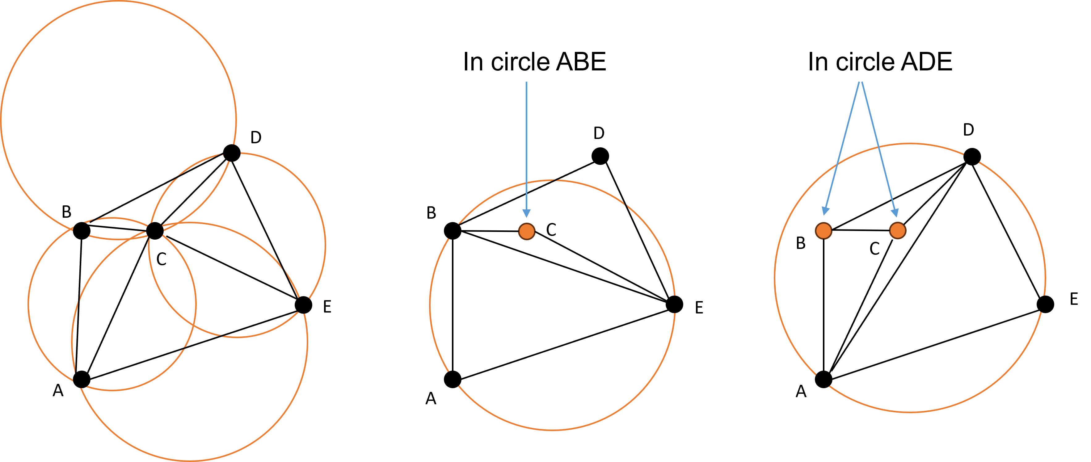
Figure 1: Example of the possible triangulations for the set of points $\{A,B,C,D,E\}$. Only the one on the left is a Delaunay triangulation.

Similar definitions follow for 3D triangulations, where the convex hull of $\mathcal{P}$ is decomposed into tetrahedra such that the vertices of tetrahedra belong to $\mathcal{P}$, and the intersection of two tetrahedra is either empty or a vertex or an edge or a face. For such a reason, a triangulation in 3D space can be called triangulation, 3D triangulation, or tetrahedralization [36].

A framework whose graph $\mathcal{G}$ is a Delaunay triangulation is rigid and the rank of the rigidity matrix is $2N-3$ (respectively $3N-6$) in $\mathbb{R}^{2}$ (respectively $\mathbb{R}^{3}$) [37].

3 Problem description

3.1 Agents model

The state of each mobile agent is described by the vector

$$p_{i}(t)=\begin{pmatrix}p_{x,i}(t)\\ p_{y,i}(t)\\ p_{z,i}(t)\end{pmatrix},$$ (1)

which represents the Cartesian coordinates.

Let the $N$ agents obey the single-integrator dynamics:

$$\dot{p}_{i}(t)=u_{i}(t),\ \ i=1,\dots,N,$$ (2)

where $u_{i}(t)\in\mathbb{R}^{3}$ are the control inputs of agent $i$, which will be described later in the paper.

We assume that each agent is equipped, at least, with hardware that allows the measurement of the distance to other agents and relative position measurements in their local coordinate frames.

3.2 Gradient control

In Krick et al. [8], a distributed control law is proposed for formation control, where the control law is derived from a potential function based on an undirected and infinitesimally rigid graph. More specifically, the potential function has the form

$$W=\frac{1}{4}\sum_{(i,j)\in\mathcal{E}}(d^{2}_{ij}-{d^{*}_{ij}}^{2})^{2},$$ (3)

where $d_{ij}=\|p_{i}-p_{j}\|$ and $d^{*}_{ij}$ is the prescribed distance for the edge $(i,j)\in\mathcal{E}$. The gradient descent control law for each agent $i$ derived from the potential function (3) is then

$$u_{i}=-\nabla_{p_{i}}W=-\sum_{j\in\mathcal{N}_{i}}(d^{2}_{ij}-{d^{*}_{ij}}^{2})(p_{i}-p_{j}).$$ (4)

It has been shown in [8] that, for a single integrator model of the agents moving in $\mathbb{R}^{2}$, the target formation is local asymptotically stable under the control law (4) if the graph of the framework is infinitesimally rigid. However, the global stability analysis beyond a local convergence for formation control systems with general shapes cannot be achieved due to the existence of multiple equilibrium sets, and a complete analysis of these sets and their stability property is very challenging due to the nonlinear control terms [16]. More specifically, even though $W=0$ in (3) only at the desired formation, i.e., when $d_{ij}=d_{ij}^{*}$, there exist other equilibria sets that correspond to $\nabla_{p_{i}}W=0$, including collinearity (in $\mathbb{R}^{2}$) and collinearity and coplanarity (in $\mathbb{R}^{3}$) of the agents.

3.3 Shield model

The team of agents should be deployed to protect a certain area of interest that, without loss of generality, is placed around the origin, i.e., $p_{0}^{*}=\mathbf{0}$. For the aforementioned purpose, the agents form a mesh with a certain shape that we call a shield. We model this “virtual” shield by a quadric surface $\mathcal{S}\in\mathbb{R}^{3}$ described in the following compact form

$$\mathcal{S}\equiv p^{\top}Q_{1}p+Q_{2}=0,$$ (5)

where $p\in\mathbb{R}^{3}$, $Q_{1}\in\mathbb{R}^{3\times 3}$ such that $Q_{1}=Q_{1}^{\top}$, and $Q_{2}\in\mathbb{R}$. Note that this is a quite general form though it excludes some shapes such as the different paraboloids or the parabolic cylinder. Additionally, since the shield is deployed around the point $p_{0}^{*}=\mathbf{0}$, we consider quadric surfaces in their normal form [38], which imposes some constraints on the values of $Q_{i}$. Furthermore, the shield might require the definition of some additional constraints for the positioning of the agents, for example, having an upper and/or lower bound on some of the coordinates, but this will be handled by the control law. In general, we constrain $z>0$. Table 1 and Figure 2 illustrate some examples of $\mathcal{S}$.

Type of shield	$\mathbf{Q_{1}}$	$\mathbf{Q_{2}}$	Constraints
Semi-ellipsoid	$\begin{pmatrix}\frac{1}{a^{2}}&0&0\\ 0&\frac{1}{b^{2}}&0\\ 0&0&\frac{1}{c^{2}}\end{pmatrix}$	$-1$	$z\geq 0$
Cylinder of height $c$	$\begin{pmatrix}\frac{1}{a^{2}}&0&0\\ 0&\frac{1}{a^{2}}&0\\ 0&0&0\end{pmatrix}$	$-1$	$c\geq z\geq 0$
Cone of height $c$	$\begin{pmatrix}\frac{1}{a^{2}}&0&0\\ 0&\frac{1}{a^{2}}&0\\ 0&0&-\frac{1}{c^{2}}\end{pmatrix}$	$-1$	$c\geq z\geq 0$

Table 1: Examples of shield models given by (5).

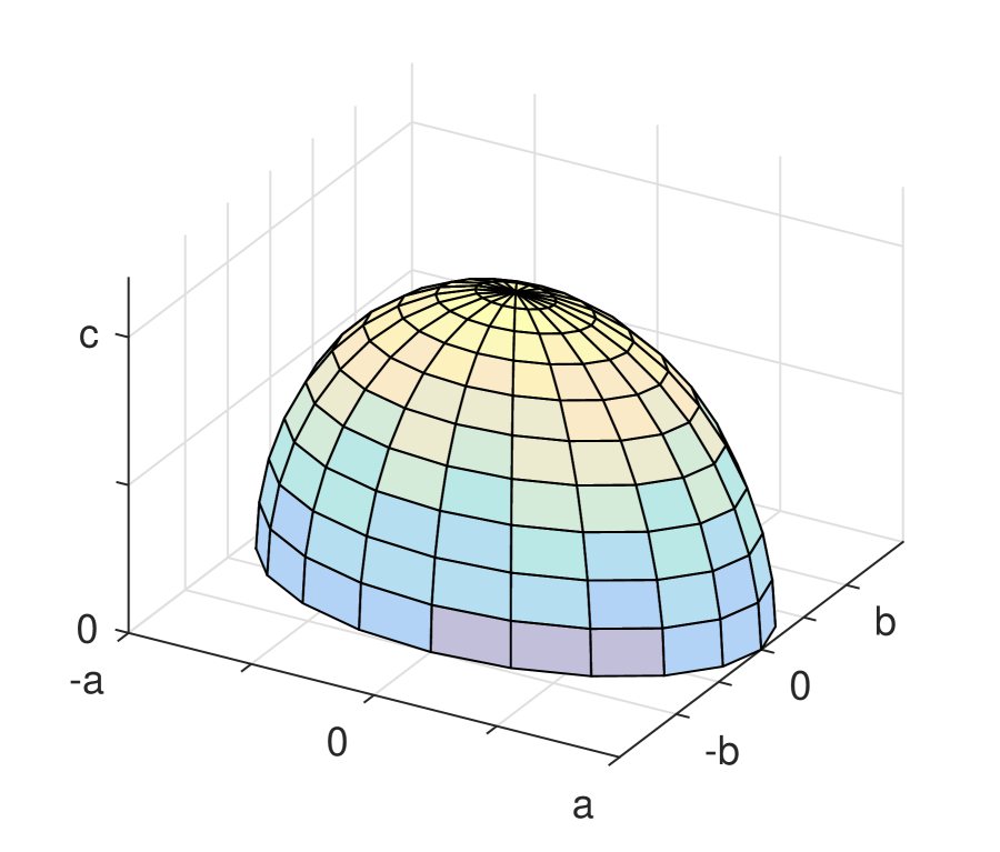
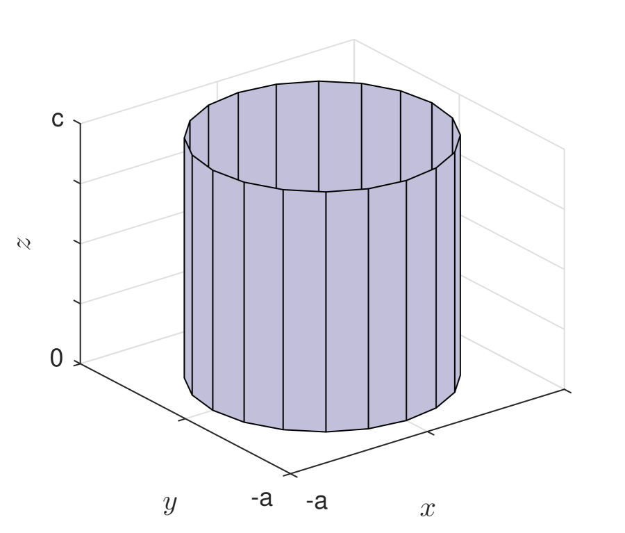
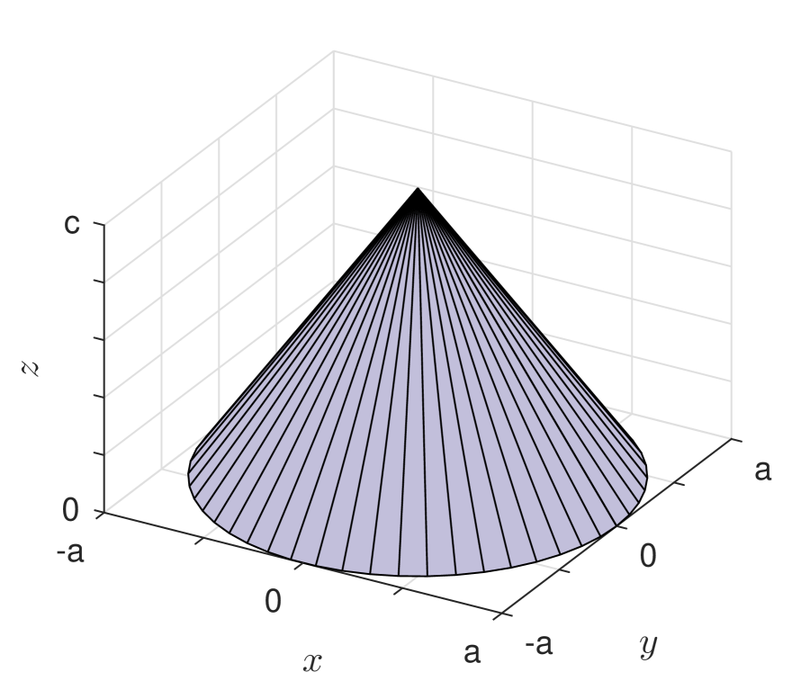
Figure 2: View of the shield examples given in Table 1: Semi-ellipsoid (left), cylinder (middle), cone (right).

For the state of an agent $i$, we can define the following function

$$f_{\mathcal{S}}(p_{i})=p_{i}^{\top}Q_{1}p_{i}+Q_{2}.$$ (6)

Note that $f_{\mathcal{S}}(p_{i})=0\iff p_{i}\in\mathcal{S}$.

3.4 Problem statement

Given the team of agents (2) and the virtual shield described by (5): I) Design an algorithm that finds a configuration (communication graph and maximum desired inter-distances between agents) that serves as a target formation so that the team is deployed forming the shield; II) design the distributed control law to achieve the desired formation.

Therefore, the solution to this problem is developed in two steps. The first one (corresponding to the first objective) is presented in Section 4; and Section 5 provides the proposed solution to the second objective.

4 Shield building

This section presents a method to design the target formation that consists of a mesh of nodes forming the shield. An example of a shield in which the virtual surface is a semi-sphere is shown in Figure 3.

First, an algorithm is proposed so that, given a desired shape, its geometry, and the number of agents, an estimation of the formation’s target distances is given such that the agents distribute more or less uniformly over the virtual surface. After that, a procedure to create the links between nodes is presented so that the result is a Delaunay triangulation.

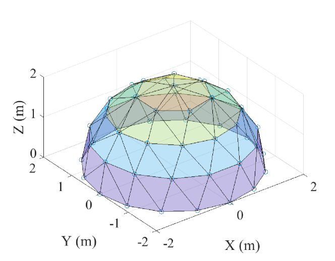
Figure 3: Target formation example. A team of $N=50$ agents forms a semi-spherical shield.

There exist in the literature many results that study how to distribute points over a sphere. The foundation of this is the so-called Thomson problem [39]: find the minimum electrostatic potential energy configuration of $N$ electrons constrained on the surface of the unit sphere, and it is being around for more than a century. This problem seems simple in its formulation, but it is one of the mathematical open problems due to the complexity of the general solution, and the computability or tractability of some simple cases. Thus, there exist solutions based on numerical analysis and approximation theory such as: Fibonacci and generalized spiral nodes; projections of low discrepancy nodes from the unit square; polygonal nodes such as icosahedral, cubed sphere, and octahedral nodes; minimal energy nodes; maximal determinant nodes; or random nodes (see [40, 41] and references therein). However, the extrapolation to other surfaces is not straightforward and requires complex mathematics that ends in different approximations [42].

Thus, the proposed method tries to find a simple procedure to provide an initial estimation of the maximum distance between agents that allows the placement of the nodes over the surface. It is based on the idea that the area of the surface, $A_{\mathcal{S}}$, is a generally well-known property that only depends on a few parameters. The idea behind this consists of approximating the area of the surface by the area of Delaunay triangles of the formation, assuming than are equilateral, to infer the distance between nodes.

For an equilateral triangle, if the distance between the points is $d$ and $h$ its height, the area is given by

$$A_{f}=\frac{d\cdot h}{2}=\tfrac{\sqrt{3}}{4}d^{2}.$$ (7)

According to the theory of rigid formations [43] the number of triangles of a Delaunay triangulation in 2D is given by

$$f=2N-2-e_{b},$$ (8)

where $e_{b}$ is the number of edges in the boundary of the triangulation. Note that even though the state space is $\mathbb{R}^{3}$, the fact that the target formation is constrained over $\mathcal{S}$, makes the previous result applies.

Thus, the area of the set of triangles is

$$f\cdot A_{f}=(2N-2-e_{b})\tfrac{\sqrt{3}}{4}d^{2}.$$ (9)

On the other hand, the number of edges in the boundary also depends on geometrical properties of the surface. For instance, if the boundary is defined by the intersection of the surface with a plane, the result is a curve whose length can be approximated by the number of nodes in the curve and the distance between them, i.e., $L_{b}\approx e_{b}\cdot d$. Actually, this is the perimeter of the boundary of the triangulation. This yields in (9) to

$$f\cdot A_{f}\approx(2N-2-\frac{L_{b}}{d})\tfrac{\sqrt{3}}{4}d^{2}.$$ (10)

If the area of the surface $A_{\mathcal{S}}$ is approximated by (10), this results on a second order equation to solve $d$:

$$A_{\mathcal{S}}\approx(2N-2-\frac{L_{b}}{d})\tfrac{\sqrt{3}}{4}d^{2}.$$ (11)

For a convex surface, (11) is actually an inequality $A_{\mathcal{S}}\geq(2N-2-\frac{L_{b}}{d})\tfrac{\sqrt{3}}{4}d^{2}$, so that

$$d\leq\frac{L_{b}+\sqrt{L_{b}^{2}+\tfrac{32}{\sqrt{3}}A_{\mathcal{S}}(N-1)}}{4(N-1)}.$$ (12)

Note that the previous procedure not only provides a value for the maximum inter-distance between nodes $d$ but the number of nodes that should be placed in the boundary, since the number of vertices of a closed path or a cycle equals the number of edges.

$$n_{b}=e_{b}=\lceil\frac{L_{b}}{d}\rceil,$$ (13)

where $\lceil x\rceil$ is the ceiling function. If we assume that the nodes are distributed on the surface in rings of different heights, the previous procedure can be repeated iteratively to determine the height and the number of nodes in each ring. The idea is as follows. Let us denote $h_{k}$ the height of the ring $k$, $A_{k}$ the area of the resulting surface over the intersection of $\mathcal{S}$ with plane $z=h_{k}$, $L_{k}$ the perimeter of such plane section and $N_{k}$ the remaining number of nodes at iteration $k$. Then, if $A_{k}$ and $L_{k}$ can be expressed in terms of $h_{k}$ and $d$ is given by (12), then an equivalent equation to (11) can be applied to get $h_{k}$:

$$A_{k}(h_{k})\approx(2N_{k}-2-\frac{L_{k}(h_{k})}{d})\tfrac{\sqrt{3}}{4}d^{2},$$ (14)

where $N_{k}$ is the number of remaining nodes. Thus, the number of nodes to be placed at the ring of height $h_{k}$ is

$$n_{k}=\lceil\frac{L_{k}}{d}\rceil.$$ (15)

Remark 1.

The ceiling operation in (15) makes that, in general, $n_{k}\cdot d>L_{k}$. Then, the parameter $d$ can be adjusted for each level $k$ as

$$d_{k}=\frac{L_{k}}{n_{k}},$$ (16)

so that all the agents can be uniformly distributed in the ring of heigh $h_{k}$. Moreover, when the algorithm is in the last step, it might occur that the number of remaining agents, $N_{k}$, satisfies that $N_{k}<n_{k}$. In that case, $n_{k}$ is set to $N_{k}$, and then $d_{k}$ is computed by (16). That way, the algorithm always guarantees a position for each node.

Algorithm 1 summarizes the iterative procedure for building the shield.

Algorithm 1 Algorithm for shield building

  

  Require: $N,A_{\mathcal{S}},L_{b}$

        Compute $d$ as (12)

        Compute $n_{b}$ as (13)

        Adjust $d_{0}$ according to $d_{0}=\frac{L_{b}}{n_{b}}$

        $k\leftarrow 1$

        $N_{k}\leftarrow N-n_{b}$

        Compute $h_{k}$ as the solution of (14)

        while $N_{k}>0$ and $h_{k}\leq h_{max}$

            Compute $n_{k}$ as (15)

            if $n_{k}>N_{k}$

                $n_{k}\leftarrow N_{k}$

            end if

            Compute $d_{k}$ as (16)

            $k\leftarrow k+1$

            $N_{k}\leftarrow N_{k}-n_{k}$

            Compute $h_{k}$ as the solution of (14)

        end while

Example 2.

Let us consider a semi-sphere of $R$=15. Let us compute the solution provided by the proposed method and estimate the error of the estimation. Table 2 shows the estimation for the distance between nodes $d$ for different values of $N$ and the error in the estimated area of the surface. The number of triangles and the number of nodes in the boundary are also given.

$N$	$d$	$f$	$e_{b}$	$(A_{\mathcal{S}}-fA_{f})/A_{\mathcal{S}}$
20	10.59	29	9	0.29
50	6.27	82	16	0.01
100	4.31	176	22	$6.28\cdot 10^{-4}$

Table 2: Values obtained for $d$ in Algorithm 1 for a semi-sphere of $R=15$ for different values of $N$.

The results show that the larger the value of $N$, the better the approximation and, of course, the shorter the distance between nodes.

Once the number of agents that should be placed in each level $h_{k}$ is computed, a simple procedure to create the edges can be followed as follows:

• Each point $i$ creates a link to the two adjacent points in the ring of height $h_{k}$: “left” ($i-1$) and “right” ($i+1$).

• Each point $i$ of the level $h_{k}$ creates a link to the points $j$ of the level $h_{k+1}$ that are at a distance $d_{ij}\leq d+\varepsilon$, where $d$ is computed by means of (12) and $\varepsilon$ is a design parameter.

• If the projection over $z=0$ of the new link $ij$ between levels $h_{k}$ and $h_{k+1}$ intersects with the projection of an existing link between these levels, the link $ij$ is removed.

• Update $d_{ij}^{*}$ to the actual value $d_{ij}$.

The previous method creates a triangulation where, in general, the triangles are not equilateral as it was assumed, at first, when computing the approximate value $d$. Hence, the target values $d_{ij}^{*}$ will be different from the initial estimation. We first assume that the resulting triangulation is Delaunay. Section 4.1 will provide a method to check this condition for each triangle.

The following result estimates the upper and lower bounds for the number of edges in a triangulation generated by the procedure described in this section.

Proposition 1.

Let us consider a network of $N$ nodes deploying a formation in form of a Delaunay triangulation over a surface $\mathcal{S}$. The number of edges of the triangulation $N_{e}$ is bounded as

$$2N-2\leq N_{e}\leq 3N-6.$$ (17)

Proof.

Similarly to (8), the number of edges is also a linear function of the number of vertices and boundary edges [43]. More specifically, and according to the Euler Formula, it holds that

$$N-e_{b}-e_{i}+f=1,$$

where $e_{i}$ are the number of edges not in the boundary. Also, it holds that $3f=e_{b}+2e_{i}$ since each non-boundary edge is shared by two faces, and then it follows that $e_{i}=3N-3-2e_{b}$.

The minimal configuration of the shield requires at least 3 nodes in the boundary so that a valid triangulation is generated (and the minimum number of nodes is $N=4$). Then, the total number of edges can be bounded as

$$N_{e}=e_{i}+e_{b}=3N-3-2e_{b}+e_{b}=3N-3-e_{b}\leq 3N-6.$$

Similarly, the maximum $e_{b}$ is $N-1$, which corresponds to having $N-1$ nodes in the boundary. Then

$$N_{e}=e_{i}+e_{b}=3N-3-e_{b}\geq 2N-2,$$

which completes the proof. ∎

4.1 Local Characterization of Delaunay Triangulations

In this section, we present a method to check if the formation of agents in form of triangulation deployed in a surface $\mathcal{S}$ (5) is Delaunay’s. The basic definitions were introduced in Section 2.4. Each of the vertices of the triangulation represents one agent $i\in\mathcal{V}$ with the coordinates $p_{i}\in\mathbb{R}^{3}$. As shown in Mathieson and Moscato [14], if the connectivity graph $\mathcal{G}$ is a Delaunay triangulation, each agent $i$ is connected to its geometrically closest neighbors.

The next analysis will provide a local characterization so that each agent $i$ can check if a triangle is Delaunay by exploiting the empty-circumcircle property of Definition 5. We particularly extend the ideas of Schwab and Lunze [30] which deal with proximity graphs in $\mathbb{R}^{2}$ to a surface $\mathcal{S}\in\mathbb{R}^{3}$ defined by (5). In Figure 4 a 2D view of a triangle and its circumcircle is depicted to illustrate the concepts. The point $m_{ABC}$ represent the circumcenter of the triangle formed by the three vertices $\{A,B,C\}$.

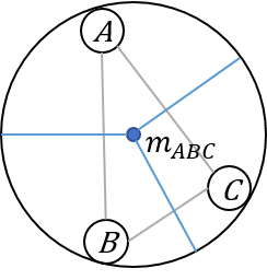
Figure 4: The triangle formed by $\{A,B,C\}$, its circumcircle, and its circumcenter $m_{123}$.

Consider the following matrix

$$O_{ABC}=\begin{pmatrix}p_{x,A}&p_{x,B}&p_{x,C}\\ p_{y,A}&p_{y,B}&p_{y,C}\\ p_{z,A}&p_{z,B}&p_{z,C}\end{pmatrix},$$ (18)

denoted as the orientation matrix. Note that $|O_{ABC}|=0$ if the three points $A$, $B$, and $C$ are collinear. Also, the three points define a plane in the space $\mathbb{R}^{3}$:

$$f_{\pi}\equiv ap_{x}+bp_{y}+cp_{z}+d=0,$$ (19)

where $a,b,c,d\in\mathbb{R}$ can actually be related to the coordinates of $p_{BA}=p_{B}-p_{A}$ and $p_{CA}=p_{C}-p_{A}$ as

$$a= \begin{vmatrix}p_{y,BA}&p_{y,CA}\\ p_{z,BA}&p_{z,CA}\end{vmatrix},\ b=-\begin{vmatrix}p_{x,BA}&p_{x,CA}\\ p_{z,BA}&p_{z,CA}\end{vmatrix},$$ (20)

$$c= \begin{vmatrix}p_{x,BA}&p_{x,CA}\\ p_{y,BA}&p_{y,CA}\end{vmatrix},\ d=-|O_{ABC}|.$$ (21)

Remark 2.

Note that if $p_{A},\ p_{B}$, and $p_{C}$ are collinear or if the origin $(0,0,0)\in f_{\pi}$ in (19), then $|O_{ABC}|=0$. However, these situations cannot occur when the distribution of points and connection between them is generated as explained at the beginning of this section. First, three points in a non-degenerate quadric surface cannot be collinear; secondly, in the case of degenerate quadrics, the alignment of three points forming a triangle is excluded in the procedure to generate the formation; and finally, the shield is deployed around the area of interest, centered at the origin, and there are not three points in the plane $p_{z}=0$ forming a triangle.

4.1.1 Circumcenter

The circumcenter of the triangle defined by the points $p_{A},p_{B}$, and $p_{C}$ is denoted by $m_{ABC}$ and satisfies the following condition:

$$\|m_{ABC}-p_{A}\|=\|m_{ABC}-p_{B}\|=\|m_{ABC}-p_{C}\|,$$ (22)

i.e., the distance from each vertex is the same. However, in $\mathbb{R}^{3}$ there are infinite points that fulfill such conditions. Therefore, the following constraint is required to compute the circumcenter: $m_{ABC}\in f_{\pi}$.

Then following result provides a method to compute it as well as the radius of the circumcircle.

Lemma 1.

The circumcenter $m_{ABC}$ of three points $p_{A}$, $p_{B}$, and $p_{C}\in\mathbb{R}^{3}$ that are not collinear is given by

$$\begin{pmatrix}m_{ABC}\\ \gamma\end{pmatrix}=\frac{1}{2}\Lambda^{-1}\begin{pmatrix}\|p_{A}\|^{2}\\ \|p_{B}\|^{2}\\ \|p_{C}\|^{2}\\ 2|O_{ABC}|\end{pmatrix},$$ (23)

where

$$\Lambda=\begin{pmatrix}O_{ABC}&\mathbf{1}\\ v^{\top}&0\end{pmatrix},$$ (24)

$\mathbf{1}=(1\ 1\ 1)^{\top}$, $\gamma$ is a scalar, and $v$ is the normal vector of the plane (19) defined by $p_{A}$, $p_{B}$ and $p_{C}$. Furthermore, the radius of the circumcircle $r_{ABC}$ is

$$r_{ABC}=\sqrt{2\gamma+\|m_{ABC}\|^{2}}.$$ (25)

Proof.

The equation (22) can be rewritten as

$$(I-P)\Bigg{(}\begin{pmatrix}\|p_{A}\|^{2}\\ \|p_{B}\|^{2}\\ \|p_{C}\|^{2}\end{pmatrix}-2\begin{pmatrix}p_{A}^{\top}\\ p_{B}^{\top}\\ p_{C}^{\top}\end{pmatrix}m_{ABC}\Bigg{)}=\mathbf{0},$$

where $P$ is a permutation matrix given by

$$P=\begin{pmatrix}0&1&0\\ 0&0&1\\ 1&0&0\end{pmatrix}.$$

Then, $I-P$ is a Laplacian matrix, and hence, $(I-P)\mathbf{1}=\mathbf{0}$, and it follows that

$$\begin{pmatrix}\|p_{A}\|^{2}\\ \|p_{B}\|^{2}\\ \|p_{C}\|^{2}\end{pmatrix}=2\begin{pmatrix}p_{A}^{\top}\\ p_{B}^{\top}\\ p_{C}^{\top}\end{pmatrix}m_{ABC}+2\gamma\begin{pmatrix}1\\ 1\\ 1\end{pmatrix}$$ (26)

for any $\gamma$. Additionally, since $m_{ABC}=(p_{x,ABC},p_{y,ABC},p_{z,ABC})\in f_{\pi}$, it holds that

$$a\cdot p_{x,ABC}+b\cdot p_{y,ABC}+c\cdot p_{z,ABC}+d=0.$$

The parameters of $f_{\pi}$ in (19) are defined in (20)-(21). Furthermore, the normal vector of $f_{\pi}$ in (19) is $v^{\top}=(a,b,c)$, and thus

$$v^{\top}m_{ABC}=|O_{ABC}|.$$ (27)

Then, we can rewrite (26) and (27) as

$$\begin{pmatrix}\|p_{A}\|^{2}\\ \|p_{B}\|^{2}\\ \|p_{C}\|^{2}\\ 2|O_{ABC}|\end{pmatrix}=2\begin{pmatrix}O_{ABC}&\mathbf{1}\\ v^{\top}&0\end{pmatrix}\begin{pmatrix}m_{ABC}\\ \gamma\end{pmatrix},$$

which proves (23).

Finally, to demonstrate (25), we recall that for $p_{i}$, $i\in\{A,B,C\}$, it holds that

$$\|p_{i}\|^{2}-2p_{i}^{\top}m_{ABC}+\|m_{ABC}\|^{2}-r_{ABC}^{2}=0.$$

Also, according to (26)

$$\|p_{i}\|^{2}-2p_{i}^{\top}m_{ABC}-2\gamma=0,$$

then (25) can be inferred. ∎

Lemma 2.

If $p_{A}$, $p_{B}$, and $p_{C}$ are not collinear and the origin $(0,0,0)\notin f_{\pi}$ defined in (19), the determinant of the matrix $\Lambda$ in (24) is always negative, i.e., $|\Lambda|<0$.

Proof.

The determinant of $\Lambda$ in (24) can be computed following the Laplace expansion as

$$|\Lambda|= -a\begin{vmatrix}p_{y,A}&p_{z,A}&1\\ p_{y,B}&p_{z,B}&1\\ p_{y,C}&p_{z,C}&1\end{vmatrix}+b\begin{vmatrix}p_{x,A}&p_{z,A}&1\\ p_{x,B}&p_{z,B}&1\\ p_{x,C}&p_{z,C}&1\end{vmatrix}$$

$$-c\begin{vmatrix}p_{x,A}&p_{y,A}&1\\ p_{x,B}&p_{y,B}&1\\ p_{x,C}&p_{y,C}&1\end{vmatrix}.$$

As the determinants above are another way of computing the parameters $a$, $-b$, and $c$, respectively, of the plane $f_{\pi}$ [44], then it follows that

$$|\Lambda|=-a^{2}-b^{2}-c^{2}<0.$$

∎

4.1.2 In-spherical cap test

To test if a triangle formed by three points $p_{A}$, $p_{B}$, and $p_{C}$ is Delaunay locally, we can check that no other node of the network, represented by $p_{D}$, satisfies that $\|p_{D}-m_{ABC}\|<r_{ABC}$. This is an extension of the incircle test [30] to our setting $\mathcal{S}\in\mathbb{R}^{3}$ (5). For that purpose, we define the following matrix

$$M_{ABCD}=\begin{pmatrix}\Lambda&v_{P}\\ \begin{pmatrix}p_{D}^{\top}&1\end{pmatrix}&\|p_{D}\|^{2}\end{pmatrix},$$ (28)

where

$$v_{P}^{\top}=(\|p_{A}\|^{2}\ \|p_{B}\|^{2}\ \|p_{C}\|^{2}\ 2|O_{ABC}|).$$ (29)

Note that $|M_{ABCD}|=0$ if $\|p_{D}-m_{ABC}\|=r_{ABC}$, since if we define $q^{\top}=(-2x_{ABC}\ -2y_{ABC}\ -2z_{ABC}\ \|m_{ABC}\|^{2}\ 1)\neq\mathbf{0}$, it holds that $M_{ABCD}\cdot q=\mathbf{0}$.

The next result shows that studying the sign of $|M_{ABCD}|$ allows to determine if a candidate point $p_{D}$ of the mesh breaks or not the condition that the triangle formed by $p_{A}$, $p_{B}$, and $p_{C}$ is Delaunay.

Theorem 1.

Consider three non-collinear points $p_{A}$, $p_{B}$, and $p_{C}$ forming a plane $f_{\pi}$ defined in (19) such that $(0,0,0)\notin f_{\pi}$, and a candidate point $p_{D}$. Let $m_{ABC}$ the circumcenter of $p_{A}$, $p_{B}$, $p_{C}$ computed as the solution of (23) and $r_{ABC}$ the radius (25) of the circumcircle. The point $p_{D}$ satisfies $\|p_{D}-m_{ABC}\|<r_{ABC}$ if $|M_{ABCD}|>0$.

Proof.

The determinant of $M_{ABCD}$ can be computed following the Laplace expansion in the last row as

$$|M {}_{ABCD}|=p_{x,D}\underbrace{\begin{vmatrix}p_{y,A}&p_{z,A}&1&\|p_{A}\|^{2}\\ p_{y,B}&p_{z,B}&1&\|p_{B}\|^{2}\\ p_{y,C}&p_{z,C}&1&\|p_{C}\|^{2}\\ b&c&0&2|O_{ABC}|\end{vmatrix}}_{|M_{1}|}-p_{y,D}\underbrace{\begin{vmatrix}p_{x,A}&p_{z,A}&1&\|p_{A}\|^{2}\\ p_{x,B}&p_{z,B}&1&\|p_{B}\|^{2}\\ p_{x,C}&p_{z,C}&1&\|p_{C}\|^{2}\\ a&c&0&2|O_{ABC}|\end{vmatrix}}_{|M_{2}|}+$$

$$p_{z,D}\underbrace{\begin{vmatrix}p_{x,A}&p_{y,A}&1&\|p_{A}\|^{2}\\ p_{x,B}&p_{y,B}&1&\|p_{B}\|^{2}\\ p_{x,C}&p_{y,C}&1&\|p_{C}\|^{2}\\ a&b&0&2|O_{ABC}|\end{vmatrix}}_{|M_{3}|}-\underbrace{\begin{vmatrix}p_{x,A}&p_{y,A}&p_{z,A}&\|p_{A}\|^{2}\\ p_{x,B}&p_{y,B}&p_{z,B}&\|p_{B}\|^{2}\\ p_{x,C}&p_{y,C}&p_{z,C}&\|p_{C}\|^{2}\\ a&b&c&2|O_{ABC}|\end{vmatrix}}_{|M_{4}|}+\|p_{D}\|^{2}|\Lambda|.$$ (30)

The four determinants $|M_{i}|$, $i=1,\dots,4$ in (4.1.2) can be expanded again using Laplace formula in the last column. For instance, for $|M_{1}|$

$$|M_{1}|= -\big{(}\|p_{A}\|^{2}(Adj(\Lambda))_{11}+\|p_{B}\|^{2}(Adj(\Lambda))_{12}$$

$$+\|p_{C}\|^{2}(Adj(\Lambda))_{13}+2|O_{ABC}|(Adj(\Lambda))_{14}\big{)},$$

where $(Adj(\Lambda))_{ij}$ refers to the element $(i,j)$ of the adjugate matrix of $\Lambda$. Note that the inverse matrix is defined as $\Lambda^{-1}=|\Lambda|^{-1}Adj(\Lambda)$. Similar expressions can be obtained for $|M_{i}|$, $i=2,3,4$, such that

$$|M_{ABCD}|= |\Lambda|\|p_{D}\|^{2}-x_{D}\sum_{j=1}^{4}(Adj(\Lambda))_{1j}(v_{p})_{j}-y_{D}\sum_{j=1}^{4}(Adj(\Lambda))_{2j}(v_{p})_{j}$$

$$-z_{D}\sum_{j=1}^{4}(Adj(\Lambda))_{3j}(v_{p})_{j}-\sum_{j=1}^{4}(Adj(\Lambda))_{4j}(v_{p})_{j},$$

where $v_{p}$ is defined in (29). Thus, from (23), it follows that

$$|M_{ABCD}|=|\Lambda|(\|p_{D}\|^{2}-2p_{D}^{\top}m_{ABC}-2\gamma).$$ (31)

The gradient of the determinant of $M_{ABCD}$ is

$$\nabla|M_{ABCD}|=2|\Lambda|(p_{D}-m_{ABC}),$$

and the Hessian matrix is

$$H(|M_{ABCD}|)=2|\Lambda|\cdot I.$$

Therefore, since $|\Lambda|$ is always negative, $|M_{ABCD}|$ is a concave function, whose maximum is at $m_{ABC}$ and $|M_{ABCD}|=0$ if $\|p_{D}-m_{ABC}\|=r_{ABC}$. Moreover, it holds that

$$|M_{ABCD}|\begin{cases}<0&\text{if }\|p_{D}-m_{ABC}\|>r_{ABC}\\ >0&\text{if }\|p_{D}-m_{ABC}\|<r_{ABC},\end{cases}$$

which completes the proof. ∎

Remark 3.

The previous result would allow to change the topology of the system dynamically if we want the condition given in Theorem 1 to be satisfied at any time while the agents are moving, but this is out of the scope of the paper. Switching topologies will be part of the future work.

Remark 4.

It must be noticed that the Delaunay extension presented in the paper is not a true 3D extension because it is not based on tetrahedrons forming the volume under the quadratic surface. The new method could be labeled as a 2D+ extension.

5 Control law

Consider the following potential function:

$$W=\frac{\kappa_{1}}{4}\sum_{(i,j)\in\mathcal{G}}(d_{ij}^{2}-d_{ij}^{*2})^{2}+\frac{\kappa_{2}}{4}\sum_{i=1}^{N}(f_{\mathcal{S}}(p_{i}))^{2},$$ (32)

where $d_{ij}=\|p_{i}-p_{j}\|$ is the distance between two agents $i$ and $j$, $d_{ij}^{*}$ is the prescribed inter-distance between both agents in the objective formation, and $\kappa_{1},\kappa_{2}\in\mathbb{R}_{>0}$. Note that (32) includes a first term corresponding to (3) and an additional term that takes into account how far each agent is from the surface $\mathcal{S}$.

Then, the distributed control law to achieve the desired objective can be computed as

$$u_{i}=-\frac{\partial W}{\partial p_{i}}=-\kappa_{1}\sum_{j\in\mathcal{N}_{i}}(d_{ij}^{2}-d_{ij}^{*2})(p_{i}-p_{j})-\frac{\kappa_{2}}{2}f_{\mathcal{S}}(p_{i})\frac{\partial f_{\mathcal{S}}(p_{i})}{\partial p_{i}}.$$ (33)

Remark 5.

At a first stage, we do not consider the constraints of the surface $\mathcal{S}$ on $z$ since we are interested on studying the analytical properties of the proposed control law. Then, we will introduce a modified control law to consider such constraints.

Let us define the error functions as

$$e_{ij}=d_{ij}^{2}-d_{ij}^{*2},$$ (34)

i.e., the error between the target distances and the square norm for the edge $ij$, or equivalently $e_{k}=\|z_{k}\|^{2}-d_{k}^{*2}$. Let us also define the following stack vectors $p^{\top}=(p_{1}^{\top},\dots,p_{N}^{\top})$, $f_{\mathcal{S}}^{\top}(p)=(f_{\mathcal{S}}(p_{1}),\dots,f_{\mathcal{S}}(p_{N}))$, and $e^{\top}=(\dots,e_{k},\dots)$. Then, (32) can be rewritten as

$$W=W_{1}+W_{2},$$ (35)

where

$$W_{1} =\frac{\kappa_{1}}{4}e^{\top}e$$ (36)

$$W_{2} =\frac{\kappa_{2}}{4}f_{\mathcal{S}}^{\top}(p)f_{\mathcal{S}}(p).$$ (37)

With the above definitions, the overall system dynamics can be rewritten as

$$\dot{p}=-\kappa_{1}R^{\top}(z)e-\kappa_{2}J_{\mathcal{S}}^{\top}(p)f_{\mathcal{S}}(p),$$ (38)

where $R(z)\equiv J_{f_{\mathcal{G}}}(p)$ is the rigidity matrix of the graph $\mathcal{G}$ and $J_{\mathcal{S}}$ is the Jacobian matrix of the function $f_{\mathcal{S}}(p)$. Note that $R(z)$ has a row for each edge and 3 (in $\mathbb{R}^{3}$) columns for each vertex, so that the $k$-th row of $R(z)$ corresponding to the $k$-th edge of $\mathcal{E}$ connecting vertices $i$ and $j$ is

$$[0\dots 0\ (p_{i}-p_{j})^{\top}0\dots 0\ (p_{j}-p_{i})^{\top}0\dots 0].$$

$J_{\mathcal{S}}$ has a block diagonal structure, such that each diagonal block $i$, $i=1,\dots,N$, is $p_{i}^{\top}Q_{1}$.

5.1 Stability analysis

In this section, we analyze the equilibria and stability of the system (2) under the control law (33). Some manipulations will be useful in the following analysis. The product $R^{\top}(z)e$ can be rewritten as $(\bar{E}(p)\otimes I_{3})p$ [45], where $\bar{E}(p)=H^{\top}E(p)H$, being $E(p)$ a diagonal matrix defined as $E(p)=diag(\dots,e_{k},\dots)$. Similarly, we can define $F_{\mathcal{S}}(p)=diag(\dots,f_{\mathcal{S}}(p_{i}),\dots)$ so that the product $J_{\mathcal{S}}^{\top}(p)f_{\mathcal{S}}(p)$ can be rewritten as $(F_{\mathcal{S}}(p)\otimes Q_{1})p$. Then, (38) is equivalent to

$$\dot{p}=-\kappa_{1}(\bar{E}(p)\otimes I_{3})p-\kappa_{2}(F_{\mathcal{S}}(p)\otimes Q_{1})p,$$ (39)

The following analysis will study the stability of the multi-agent system (2) under the control law (33).

Lemma 3.

The multi-agent system (2) with control law (33) has an equilibrium set $\mathcal{M}_{d}$ defined by

$$\mathcal{M}_{d}=\{e=0,f_{\mathcal{S}}(p)=0\}$$ (40)

corresponding to the control objective, i.e., acquisition of the desired formation defined by the prescribed distances $d_{ij}^{*}$ and placement of the agents over the virtual surface $\mathcal{S}$ defined by (5).

Proof.

The control objective is satisfied if and only if

1. $d_{ij}=d_{ij}^{*},\ \forall(i,j)\in\mathcal{E}$

2. $f_{\mathcal{S}}(p_{i})=0,\ \forall i=1,\dots,N.$

Then, the Lyapunov function (32) is 0 if and only if the control objective is achieved. Moreover, the time derivative of the Lyapunov function along the system solution is

$$\dot{W}=\big{(}\frac{\partial W_{1}}{\partial p}+\frac{\partial W_{2}}{\partial p}\big{)}\dot{p}=\big{(}\frac{\kappa_{1}}{2}e^{\top}\frac{\partial e}{\partial p}+\frac{\kappa_{2}}{2}f_{\mathcal{S}}^{\top}(p)\frac{\partial f_{\mathcal{S}}(p)}{\partial p}\big{)}\cdot\dot{p}.$$

Note that by definition the partial derivatives are the Jacobian matrices defined above, i.e., $R(z)$ and $J_{\mathcal{S}}$, respectively, then it holds that

$$\dot{W}=-\big{(}\kappa_{1}e^{\top}R(z)+\kappa_{2}f_{\mathcal{S}}^{\top}(p)J_{\mathcal{S}}(p)\big{)}\big{(}\kappa_{1}R^{\top}(z)e+\kappa_{2}J_{\mathcal{S}}^{\top}(p)f_{\mathcal{S}}(p)\big{)},$$

hence

$$\dot{W}=-\|\kappa_{1}R^{\top}(z)e+\kappa_{2}J_{\mathcal{S}}^{\top}(p)f_{\mathcal{S}}(p)\|^{2}\leq 0.$$

Then, the Lyapunov function (32) is not increasing along the system solutions, and $\dot{W}=0$ at the equilibrium set defined in (40). Hence, the proof is completed. ∎

Remark 6.

Note that the complete set of equilibria of (38) is defined by

$$\mathcal{M}=\{p:\ \kappa_{1}R^{\top}(z)e+\kappa_{2}J_{\mathcal{S}}^{\top}(p)f_{\mathcal{S}}(p)=0\},$$ (41)

such that $\mathcal{M}_{d}\subset\mathcal{M}$.

The fact that other equilibria sets exist also occurs in the problem of rigid formations [8, 16], and the conditions to facilitate the demonstration of the local stability relies on imposing the conditions of minimal and infinitesimal rigidity of the framework (see Section 2.3). However, this applies when the formation is realized in the state space $\mathbb{R}^{2}$/$\mathbb{R}^{3}$. In the setup presented in this paper, two main differences makes that the results are not applicable. First, the state of the agents $p_{i}\in\mathbb{R}^{3}$ but the formation is embedded in a virtual surface $\mathcal{S}$ of dimension 2. And secondly, constraining the formation to $\mathcal{S}$ makes that the concept of infinitesimally rigid cannot be applied as such. Actually, the rigid body motions corresponding to the translation along the axes cannot longer occur, and the rotations about one or more axes depend on the symmetries of $\mathcal{S}$.

Furthermore, note that an augmented matrix and state vector can be constructed as:

$$J_{R\mathcal{S}}^{\top}(p,z) =\begin{pmatrix}\kappa_{1}R^{\top}(z)&\kappa_{2}J_{\mathcal{S}}^{\top}(p)\end{pmatrix}$$ (42)

$$\xi^{\top}(p,z) =\begin{pmatrix}e(z)^{\top}&f_{\mathcal{S}}^{\top}(p)\end{pmatrix},$$ (43)

such that studying the rank of $J_{R\mathcal{S}}(p,z)\in\mathbb{R}^{(N_{e}+N)\times 3N}$ in this setup is equivalent to study the rank of the rigidity matrix in the classical problem of rigid formations. Actually, the non-zero elements of $J_{\mathcal{S}}$ can be seen as a square distance from the $N$ nodes to a virtual node at the origin weighted by the matrix $Q_{1}$, and then the number of edges (real plus virtual) is $N_{e}+N$. According to 1, $N_{e}+N$ belongs to the interval $[3N-2,4N-6]$. Note that if we include this virtual node (labeled as $0$ and corresponding to the origin) in the counting of vertices, $\mathcal{V}^{\prime}=\mathcal{V}\cup{0}$, such that the number of nodes is $N^{\prime}=N+1$ and then the number of edges is $N^{\prime}_{e}\in[3N^{\prime}-5,4N^{\prime}-9]$. Then, the framework is not minimally rigid under this transformation of the problem, and this can also be inferred from the results of Proposition 1, as we will discuss next in the paper.

We next analyze the rank of $J_{R\mathcal{S}}(p,z)$. Note that since the quadric surface (5) is assumed to be expressed in normal form, $Q_{1}$ has diagonal form such that $Q_{1}=diag(q_{1},q_{2},q_{3})$ (see Table 1).

Lemma 4.

The rank of $J_{R\mathcal{S}}(p,z)$ in (42) for a rigid framework defined by a Delaunay Triangulation and embedded in a surface $\mathcal{S}$ defined as (5) is at least $3N-3$. Moreover, when then number of edges of $\mathcal{G}$, is such that $N_{e}\geq 2N$, then it holds that

$$rank(J_{R\mathcal{S}})=3N-s,$$ (44)

where $s$ reflects the symmetries of $\mathcal{S}$ such that

$$s=\begin{cases}0&\text{ if }q_{i}\neq q_{j},\ \forall i\neq j,\ i,j\in\{1,2,3\}\\ 1&\text{ if }\exists i,j,k\in\{1,2,3\}\ q_{i}=q_{j},q_{i}\neq q_{k}\ i\neq j\neq k,\\ 3&\text{ if }q_{i}=q_{j}\ \forall i,j\in\{1,2,3\}.\end{cases}$$ (45)

Proof.

The rank of $J_{R\mathcal{S}}$ is $rank(J_{R\mathcal{S}}(p,z))\leq rank(R(z))+rank(J_{\mathcal{S}}(p))$, and the kernel $ker(J_{R\mathcal{S}})=ker(R(z))\cap ker(J_{\mathcal{S}})$ [46]. The rank of $R(z)=N_{e}$ since the number of edges is in the interval $[2N-2,3N-6]$ according to Proposition 1 and the graph $\mathcal{G}$ is a Delaunay triangulation to be embedded in $\mathcal{S}$ but with $z_{i}\in\mathbb{R}^{3}$. Moreover, the rank of $J_{\mathcal{S}}(p)$ is $N$ due to its block diagonal structure. Then, when the number of edges is minimal ($N_{e}=2N-2$), then $rank(J_{R\mathcal{S}})\leq 2N-2+N=3N-2$.

Moreover, we know that rigid body motions are in the kernel of $R(z)$, that is, $R(z)v=0$, such that $v^{\top}=(v_{1}^{\top},\dots,v_{N}^{\top})$ and $v_{i}=v_{0}+\omega\times p_{i}$, $i=1\dots,N$, where $v_{0}\in\mathbb{R}^{3}$ is a translational velocity and $\omega\in\mathbb{R}^{3}$ is an angular velocity. However, it is easy to see that $J_{\mathcal{S}}(p)(1_{N}\otimes v_{0})\neq 0$ for $v_{0}\neq 0$, and that for the angular velocity it holds for each block that

$$p_{i}^{\top}Q_{1}(\omega\times p_{i})=Q_{1}p_{i}\cdot(\omega\times p_{i})=\omega\cdot(Q_{1}p_{i}\times p_{i}),$$ (46)

which is not zero for the general case. However, we distinguish the following cases:

• If $Q_{1}=\alpha I_{3}$, $\alpha\in\mathbb{R}_{>0}$, then (46) is 0 $\forall\omega\in\mathbb{R}^{3}$, which corresponds to $s=3$ in (45). Then, $rank(J_{R\mathcal{S}})=3N-3$ independently of the number of edges of the triangulation if $\mathcal{S}$ is symmetric in the three axes.

• If $Q_{1}$ has some $q_{i}=q_{j}$ but $q_{k}\neq q_{i}$ for one of the axes, then (46) is 0 if $\omega_{i}=\omega_{j}=0$ but $\omega_{k}\neq 0$, That is, the components of $\omega$, corresponding to the axes in which $\mathcal{S}$ is symmetric, are zero (case $s=1$ in (45)). In that case, $rank(J_{R\mathcal{S}})=N_{e}+N-1$ if $N_{e}\leq 2N$ and $3N-1$ otherwise.

• If $\mathcal{S}$ is not symmetric in any of the axes, then (46) is not zero, and then the intersection of the kernels of $R(z)$ and $J_{\mathcal{S}}(p)$ is $\emptyset$ and then $rank(J_{R\mathcal{S}})=min(N_{e}+N,3N)$.

Then, the proof is completed. ∎

We finally present the main result of this section regarding stability based on the previous developments.

Theorem 2.

The multi-agent system (2) for a given shield model described by (5), the graph constructed such that the target formation is a Delaunay triangulation over $\mathcal{S}$, and the control law (33), is locally exponentially stable at the desired relative positions $d_{ij}^{*}$ over the surface $\mathcal{S}$ corresponding to $e=0$ and $f_{\mathcal{S}}(p)=0$.

Proof.

According to Lemma 3, the Lyapunov function is not increasing along the systems solutions of the system and (40) is an equilibrium set. Thus, the control objective is locally reached exponentially if (40) is a minimum of the Lyapunov function (32).

Studying the Hessian matrix of a function provides information about the nature of a critical point. More specifically, if the Hessian of $W$, $H_{W}$, at the critical point $p^{*}\in\mathcal{M}_{d}$ is a positive-definite matrix, then $p^{*}$ is a local minimum. Thus, the Hessian matrix of the Lyapunov function (32) is the Jacobian of $\nabla W$. According to Lemma 3, $\nabla W=\kappa_{1}e^{\top}R(z)+\kappa_{2}f_{\mathcal{S}}(p)^{\top}J_{\mathcal{S}}(p)=\xi^{\top}J_{R\mathcal{S}}$. Thus

$$H_{W}=\frac{\partial\xi^{\top}}{\partial p}J_{R\mathcal{S}}+\xi^{\top}\frac{\partial J_{R\mathcal{S}}}{\partial p}.$$

If we evaluate $H_{W}$ at the critical point $p^{*}$, i.e, when $\xi=0$, the second term is 0. Moreover, it holds that

$$\frac{\partial\xi^{\top}}{\partial p}=\Big{(}\frac{\partial e^{\top}}{\partial p}\ \ \frac{\partial f_{\mathcal{S}}^{\top}}{\partial p}\Big{)}=2\Big{(}R^{\top}(z)\ \ J_{\mathcal{S}}^{\top}(p)\Big{)}$$

Then, the Hessian at $p^{*}$ is

$$H_{W}(p^{*})=2\begin{pmatrix}R^{\top}(z^{*})&J_{\mathcal{S}}^{\top}(p^{*})\end{pmatrix}\begin{pmatrix}\kappa_{1}R(z^{*})\\ \kappa_{2}J_{\mathcal{S}}(p^{*})\end{pmatrix}.$$ (47)

We can define a matrix similar to $J_{R\mathcal{S}}$ but with different weights in its blocks as

$$\tilde{J}_{R\mathcal{S}}^{\top}(p,z)=\begin{pmatrix}\sqrt{\kappa_{1}}R^{\top}(z)&\sqrt{\kappa_{2}}J_{\mathcal{S}}^{\top}(p)\end{pmatrix}.$$

The rank of $\tilde{J}_{R\mathcal{S}}$ is the same than the rank of $J_{R\mathcal{S}}$, which is analyzed in Lemma 4. Thus, the Hessian matrix (47) can be rewritten as

$$H_{W}(p^{*})=2\tilde{J}_{R\mathcal{S}}^{\top}(p^{*},z^{*})\tilde{J}_{R\mathcal{S}}(p^{*},z^{*}).$$ (48)

Note that $H_{W}(p^{*})\in\mathbb{R}^{3N\times 3N}$ is positive or semipositive definite by construction since any matrix $M$ of the form $M=B^{\top}B$, with $B$ real, is positive or semipositive definite, and $rank(M)=rank(B)$. More specifically, if $rank(\tilde{J}_{R\mathcal{S}})=rank(J_{R\mathcal{S}})=3N$ then $H_{W}(p^{*})$ is positive definite. According to Lemma 4 this is the case when $N_{e}\geq 2N$ and the surface (5) has no symmetries. In that case, we can conclude that $p^{*}$ is a locally stable critical point.

We next analyze the cases in which the surface (5) has one or more symmetries (cases $s=1,3$ in (45)) and $N_{e}\geq 2N$. In these cases, the dimension of the kernel of $J_{R\mathcal{S}}$ is $s$, $H_{W}(p^{*})$ has $s$ 0 eigenvalues and, therefore, is semi-positive definite so that we cannot conclude in principle that $p^{*}$ is a local minimum. However, in such case, a similar analysis can be applied as Theorem 4 in [8] taking into account the following issues:

• Since $1\otimes v$ is not an eigenvector of $J_{R\mathcal{S}}$, the dynamics of $p$ does not contain any component that is stationary, so a reduced version of $p$ is not required.

• The linearized dynamics of the system (38) at $p^{*}$ is

  $$\delta p=-H_{W}(p^{*})p,$$

  and the dynamics of $p$ near $p^{*}$ is

  $$\dot{p}=-H_{W}(p^{*})p-(f(p)-H_{W}(p^{*})p)$$

  where $f(p)=J_{R\mathcal{S}}(p,z)\xi(p,z)$. An orthonormal transformation $Q$ can be applied to $H_{W}(p^{*})$ such that $QH_{W}(p^{*})Q^{\top}$ is in block diagonal form with the first block of dimension $\mathbb{R}^{s\times s}$ of zeros and a second block $B\in\mathbb{R}^{(3N-s)\times(3N-s)}$ which is Hurwitz.

Then, the center manifold theory can be applied since the system can be expressed in normal form. Finally, similar arguments follow when the number of edges is $N_{e}<2N$, since also the kernel of $H_{W}(p^{*})$ will have at most dimension 3. ∎

5.2 Truncated surfaces

To deal with the constraints on the $z$ axis, which may result in truncated surfaces, we introduce an additional term in the control law by adapting classical techniques for obstacle avoidance [47]. More specifically, a repulsive potential field is defined to avoid that agents’ trajectories cross the plane $z=0$:

$$U_{r}(p_{z})=\begin{cases}\frac{\kappa_{3}}{2}\Big{(}\frac{1}{p_{z}}-\frac{1}{\epsilon}\Big{)}^{2}&\text{ if }p_{z}\leq\epsilon\\ 0&\text{ if }p_{z}>\epsilon,\end{cases}$$

where $\epsilon>0$ acts as a threshold to activate the repulsive potential field. The corresponding control term is

$$u_{r_{i}}=-\nabla U_{r}(p_{z,i})=\begin{cases}\kappa_{3}\Big{(}\frac{1}{p_{z,i}}-\frac{1}{\epsilon}\Big{)}\frac{1}{p_{z,i}^{2}}&\text{ if }p_{z,i}\leq\epsilon\\ 0&\text{ if }p_{z,i}>\epsilon.\end{cases}$$ (49)

Assuming that the initial conditions are such that $p_{z,i}(0)\geq 0$, (49) guarantees that $p_{z,i}(t)>0,\ \forall t$. Then, the control law (33) is transformed into

$$u_{i}= -\kappa_{1}\sum_{j\in\mathcal{N}_{i}}(d_{ij}^{2}-d_{ij}^{*2})(p_{i}-p_{j})-\frac{\kappa_{2}}{2}f_{\mathcal{S}}(p_{i})\frac{\partial f_{\mathcal{S}}(p_{i})}{\partial p_{i}}$$

$$+u_{r,i}.$$ (50)

Remark 7.

If the surface $\mathcal{S}$ has another constraint on $z$ such as some of the examples presented in Table 1 ($p_{z}\leq h$), the problem is solved adding a new term similar to (49) but replacing $p_{z,i}$ by $h-p_{z,i}$ and assuming that $p_{z,i}(0)\leq h$.

6 Simulation and experimental results

6.1 Simulation example 1

Let us consider a team of $N=50$ agents and a semi-ellipsoid as desired shield shape as follows:

$$\frac{x^{2}}{10^{2}}+\frac{y^{2}}{15^{2}}+\frac{z^{2}}{12^{2}}=1.$$ (51)

The execution of Algorithm 1 gives, as a result, a value for the distance between neighbors of $d=5.154$, and a distribution of levels as shown in Table 3. The lowest level denoted as $h=0$ is a practical simplification since there exists the repulsive potential field at $z=0$ (see Section 5.2), and then the height of this level should be $h>\epsilon$. Since $\epsilon$ is a small value, this does not affect the calculations.

$h_{k}$	$0^{*}$	5.078	8.422	10.750	11.938
$n_{k}$	16	14	11	7	2
$d_{k}$	4.958	5.134	5.137	5.042	4.039

Table 3: Values obtained for $h_{k}$, $N_{k}$, and $d_{k}$ in Algorithm 1 for the semi-ellipsoid defined in (51) and $N=50$.

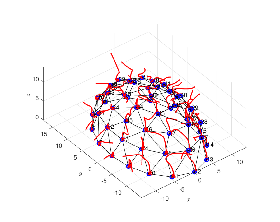
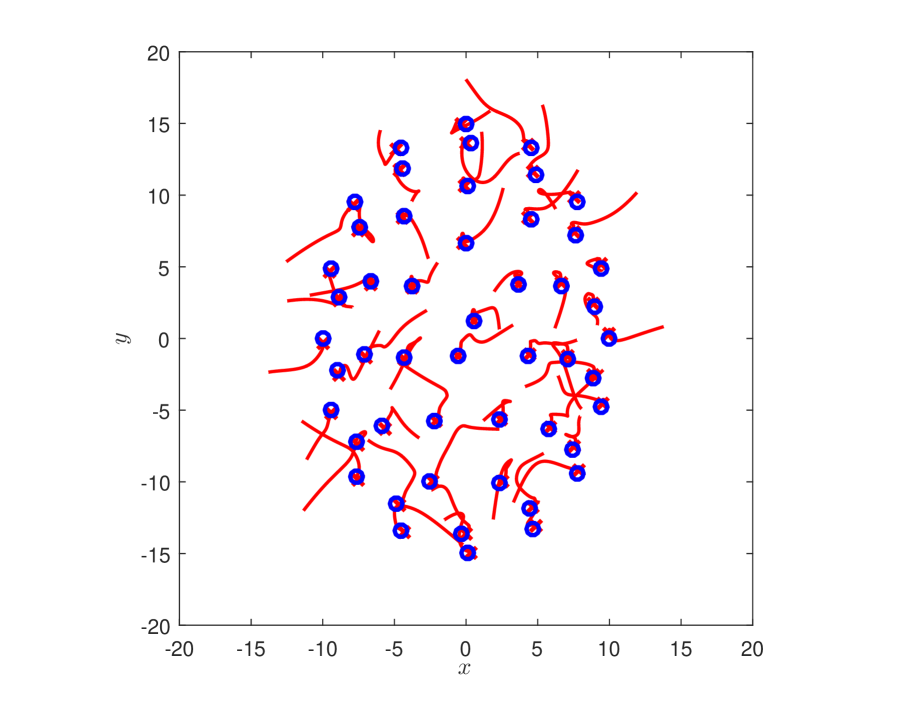
Figure 5: 3D view (left) and projection over the XY plane (right) of the trajectories of the system (in red) for Example 1. Blue circles represent positions at which errors $e_{ij}$ are 0.

The left of Figure 5 shows the trajectories of the agents in the 3D space when the initial conditions are generated randomly but with a bound such that $|d_{ij}(0)-d_{ij}^{*}|\leq 7$ for all neighboring agents $i$ and $j$, and $|f_{\mathcal{S}}(p_{i}(0))|\leq 7$. The control law (5.2) with feedback gains $\kappa_{1}=1,\ \kappa_{2}=100,\ \kappa_{3}=10^{-3}$ is applied. The topology of the system in the form of Delaunay triangulation is also depicted. The right of Figure 5 shows the projection of those trajectories over the XY plane. Note that the agents converge to the surface and they acquire the desired target distance between neighboring nodes.

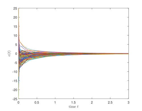
Figure 6: Evolution of the error to target distances over time for Example 1.

Figure 6 shows the evolution of the error $e$ over time. Note that the error for edges converges to 0. Let us define the total relative error to formation for the edge $k$ $e_{r,k}=\tfrac{|e_{k}|}{d_{k}^{2}}$, and the stacked vector $e_{k}=(\dots e_{r,k}\dots)^{\top}$. Then, the initial value at $t=0$ is $\|e_{r}(0)\|=26.80$, whereas we obtain $\|e_{r}(3)\|=0.075$ at $t=3$. Moreover, if the norm of the vector of distances to surface $f_{\mathcal{S}}$ is computed at $t=0$ and $t=3$, the following values are obtained: $\|f_{\mathcal{S}}(0)\|=3.80$ and $\|f_{\mathcal{S}}(3)\|=0.029$, respectively.

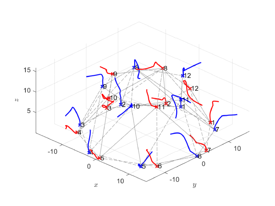
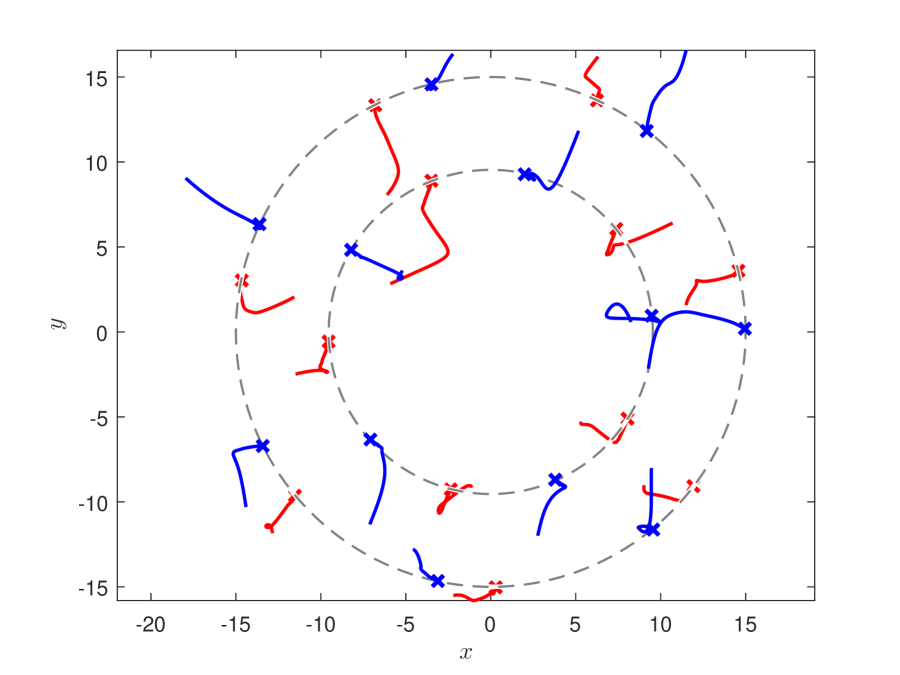
Figure 7: 3D view (left) and projection over the XY plane (right) of the trajectories of the system (in red) for two different initial conditions (Example 2). Dashed circles represent the rings of height $h=0$ and $h=3.421$.

6.2 Simulation example 2

To illustrate the results when the surface presents symmetries, let us consider the case of a semi-sphere with $R=15$ and a multi-agent system with $N=12$. In this case, Algorithm 1 distributes the agents in two rings with 7 and 5 drones at heights $h=0^{*}$ (similar comments as the previous example applies) and $h=3.421$, respectively. The left of Figure 7 shows the trajectories and the topology of the system in the 3D space for two different initial conditions. For the data in red, the norm of the relative errors’ vector at the end of the experiment is $\|e_{r}(3)\|=0.002$, and the norm of $f_{\mathcal{S}}$ is $\|f_{\mathcal{S}}(3)\|=0.023$. For the data in blue, $\|e_{r}(3)\|=0.002$ and $\|f_{\mathcal{S}}(3)\|=0.022$. Then, the control objective is achieved in both cases but the final positions differ (there exists a rotation) influenced by the initial conditions. The projection of the trajectories over the XY plane is depicted on the right of Figure 7. Dashed circles represent the rings of height $h=0$ and $h=3.421$ that Algorithm 1 computes to ensure an almost uniform distribution of the nodes.

6.3 Real-time experiment

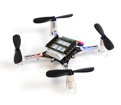
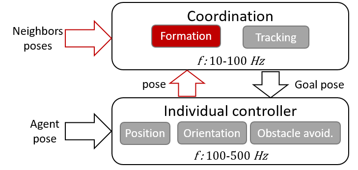
Figure 8: Crazyflie 2.1 (left), hierarchical control architecture (right).

The proposed strategy has also been tested over the experimental platform described in Mañas-Álvarez et al. [31], which supports different autonomous robots including UAVs. Demo videos of the platform can be found at https://youtu.be/4H3YZ-sr2mw. A team of 5 micro-aerial quadcopter Crazyflie 2.1 [48] (see Figure 8 left) has been used for the experiments presented in this paper. The robot has a STM32F405 microcontroller and a Bluetooth module that allows the communication. The Crazyflie uses its own positioning system, the Lighthouse [49], which is based on infrared laser and enables the Crazyflie to calculate its own position onboard with a precision of 1 mm. The control architecture follows a hierarchical scheme (see Figure 8 right) so that the proposed control law in this paper is applied in the upper level (coordination) and provides a goal pose to the individual controller. The low-level controller of each quadrotor is responsible for moving the vehicle to the desired pose with the yaw angle set to zero.

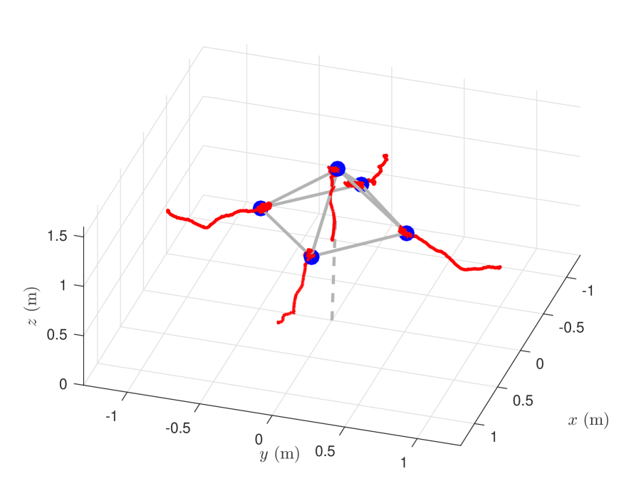
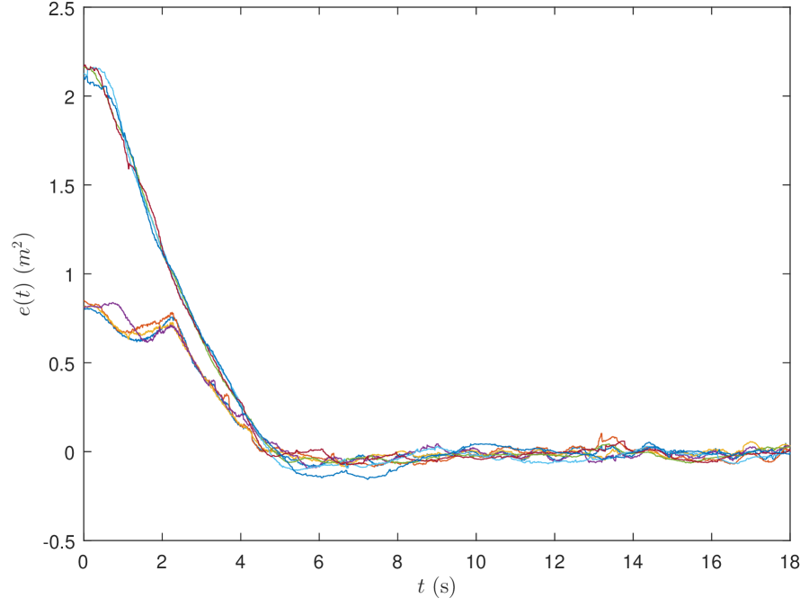
Figure 9: 3D view of the trajectories of the team of 5 Crazyflies 2.1 (left) and evolution of the error to target distances for the 8 edges of the graph (right).

The virtual surface is a semisphere with $R=0.5$ m, whose center is at $(0,0,1)$ m, and the target distances are all set to $d^{*}_{ij}=0.7$ m for the 8 edges of the graph $(i,j)\in\mathcal{E}$. The robots are first commanded to move to the plane $z_{0}=0.7$ m, and then the coordination controller starts working. The trajectories of the robots are depicted on the left of Figure 9. The right of Figure 9 shows the evolution of the error of the formation over time, where it is clear that the multi-agent system converges to the desired formation.

7 Conclusions

In this paper, we have studied the formation shape control problem of a set of agents moving in the 3D space. They should achieve a formation in such a way that they form a shield and are distributed over a virtual surface modeled as a quadric in normal form. The potential application is the protection of an area of interest and the monitoring of external threats. An algorithm has been proposed to guarantee an almost uniform distribution of the nodes and the network configuration in the form of a Delaunay triangulation. A method to test if each triangle is Delaunay has been designed, so that it can be executed locally. Moreover, a distributed control law has been proposed to guarantee the achievement of the control objective. Although the conditions of minimal and infinitesimal rigidity of the framework do not hold in our setting, we have been able to provide proofs of local stability. The simulation and experimental results have shown that the proposed control method yields asymptotic stability of the desired formation.

Although the analysis of this paper was centered on single integrator agents, we have been able to apply it to UAVs thanks to a hierarchical control architecture. However, the extension of the proposed approach to more detailed UAV models will be part of future work. Also, we will study switching topologies and the design of strategies to handle disturbances and failures in the system (loss of agents or sensing capacities).

References

- Leonard et al. [2007] N. E. Leonard, D. A. Paley, F. Lekien, R. Sepulchre, D. M. Fratantoni, R. E. Davis, Collective motion, sensor networks, and ocean sampling, Proceedings of the IEEE 95 (2007) 48–74.
- Fidan et al. [2007] B. Fidan, C. Yu, B. D. Anderson, Acquiring and maintaining persistence of autonomous multi-vehicle formations, IET Control Theory & Applications 1 (2007) 452–460.
- Aranda et al. [2015] M. Aranda, G. López-Nicolás, C. Sagüés, Y. Mezouar, Formation control of mobile robots using multiple aerial cameras, IEEE Transactions on Robotics 31 (2015) 1064–1071.
- Fredslund and Mataric [2002] J. Fredslund, M. J. Mataric, A general algorithm for robot formations using local sensing and minimal communication, IEEE Transactions on Robotics and Automation 18 (2002) 837–846.
- Lawton et al. [2003] J. R. Lawton, R. W. Beard, B. J. Young, A decentralized approach to formation maneuvers, IEEE Transactions on Robotics and Automation 19 (2003) 933–941.
- Oh et al. [2015] K.-K. Oh, M.-C. Park, H.-S. Ahn, A survey of multi-agent formation control, Automatica 53 (2015) 424–440.
- Olfati-Saber and Murray [2004] R. Olfati-Saber, R. M. Murray, Consensus problems in networks of agents with switching topology and time-delays, IEEE Transactions on automatic control 49 (2004) 1520–1533.
- Krick et al. [2009] L. Krick, M. E. Broucke, B. A. Francis, Stabilisation of infinitesimally rigid formations of multi-robot networks, International Journal of Control 82 (2009) 423–439.
- Cao et al. [2011] M. Cao, C. Yu, B. D. Anderson, Formation control using range-only measurements, Automatica 47 (2011) 776–781.
- Kwon et al. [2022] S.-H. Kwon, Z. Sun, B. D. Anderson, H.-S. Ahn, Sign rigidity theory and application to formation specification control, Automatica 141 (2022) 110291.
- Mou et al. [2015] S. Mou, M.-A. Belabbas, A. S. Morse, Z. Sun, B. D. Anderson, Undirected rigid formations are problematic, IEEE Transactions on Automatic Control 61 (2015) 2821–2836.
- Anderson et al. [2008] B. D. Anderson, C. Yu, B. Fidan, J. M. Hendrickx, Rigid graph control architectures for autonomous formations, IEEE Control Systems Magazine 28 (2008) 48–63.
- De Marina et al. [2014] H. G. De Marina, M. Cao, B. Jayawardhana, Controlling rigid formations of mobile agents under inconsistent measurements, IEEE Transactions on Robotics 31 (2014) 31–39.
- Mathieson and Moscato [2019] L. Mathieson, P. Moscato, An introduction to proximity graphs, Business and Consumer Analytics: New Ideas (2019) 213–233.
- Hjelle and Dæhlen [2006] Ø. Hjelle, M. Dæhlen, Triangulations and applications, Springer Science & Business Media, 2006.
- Sun et al. [2015] Z. Sun, U. Helmke, B. D. O. Anderson, Rigid formation shape control in general dimensions: an invariance principle and open problems, in: 2015 54th IEEE Conference on Decision and Control (CDC), 2015, pp. 6095–6100.
- Dörfler and Francis [2010] F. Dörfler, B. Francis, Geometric analysis of the formation problem for autonomous robots, IEEE Transactions on Automatic Control 55 (2010) 2379–2384.
- Anderson et al. [2010] B. D. Anderson, C. Yu, S. Dasgupta, T. H. Summers, Controlling four agent formations, IFAC Proceedings Volumes 43 (2010) 139–144.
- Fathian et al. [2019] K. Fathian, N. R. Gans, W. Z. Krawcewicz, D. I. Rachinskii, Regular polygon formations with fixed size and cyclic sensing constraint, IEEE Transactions on Automatic Control 64 (2019) 5156–5163.
- Liu and de Queiroz [2020] T. Liu, M. de Queiroz, Distance+ angle-based control of 2-d rigid formations, IEEE transactions on cybernetics 51 (2020) 5969–5978.
- Anderson et al. [2017] B. D. Anderson, Z. Sun, T. Sugie, S.-i. Azuma, K. Sakurama, Formation shape control with distance and area constraints, IFAC Journal of Systems and Control 1 (2017) 2–12.
- Summers et al. [2011] T. H. Summers, C. Yu, S. Dasgupta, B. D. Anderson, Control of minimally persistent leader-remote-follower and coleader formations in the plane, IEEE Transactions on Automatic Control 56 (2011) 2778–2792.
- Brandão and Sarcinelli-Filho [2016] A. S. Brandão, M. Sarcinelli-Filho, On the guidance of multiple UAV using a centralized formation control scheme and delaunay triangulation, Journal of Intelligent & Robotic Systems 84 (2016) 397–413.
- Park et al. [2014] M.-C. Park, Z. Sun, B. D. Anderson, H.-S. Ahn, Stability analysis on four agent tetrahedral formations, in: 53rd IEEE Conference on Decision and Control, IEEE, 2014, pp. 631–636.
- Ramazani et al. [2016] S. Ramazani, R. Selmic, M. de Queiroz, Rigidity-based multiagent layered formation control, IEEE Transactions on Cybernetics 47 (2016) 1902–1913.
- Park et al. [2017] M.-C. Park, Z. Sun, B. D. Anderson, H.-S. Ahn, Distance-based control of formations in general space with almost global convergence, IEEE Transactions on Automatic Control 63 (2017) 2678–2685.
- Liu and de Queiroz [2021] T. Liu, M. de Queiroz, An orthogonal basis approach to formation shape control, Automatica 129 (2021) 109619.
- Han et al. [2017] T. Han, Z. Lin, R. Zheng, M. Fu, A barycentric coordinate-based approach to formation control under directed and switching sensing graphs, IEEE Transactions on cybernetics 48 (2017) 1202–1215.
- Han et al. [2016] T. Han, Z. Lin, Y. Xu, R. Zheng, H. Zhang, Formation control of heterogeneous agents over directed graphs, in: 2016 IEEE 55th Conference on Decision and Control (CDC), IEEE, 2016, pp. 3493–3498.
- Schwab and Lunze [2021] A. Schwab, J. Lunze, A distributed algorithm to maintain a proximity communication network among mobile agents using the delaunay triangulation, European Journal of Control 60 (2021) 125–134.
- Mañas-Álvarez et al. [2023] F. J. Mañas-Álvarez, M. Guinaldo, R. Dormido, S. Dormido, Robotic park. multi-agent platform for teaching control and robotics, IEEE Access (2023).
- Fathian et al. [2019] K. Fathian, S. Safaoui, T. H. Summers, N. R. Gans, Robust 3d distributed formation control with collision avoidance and application to multirotor aerial vehicles, in: 2019 International Conference on Robotics and Automation (ICRA), IEEE, 2019, pp. 9209–9215.
- Godsil and Royle [2001] C. Godsil, G. F. Royle, Algebraic graph theory, volume 207, Springer Science & Business Media, 2001.
- Asimow and Roth [1979] L. Asimow, B. Roth, The rigidity of graphs, II, Journal of Mathematical Analysis and Applications 68 (1979) 171–190.
- Delaunay et al. [1934] B. Delaunay, et al., Sur la sphere vide, Izv. Akad. Nauk SSSR, Otdelenie Matematicheskii i Estestvennyka Nauk 7 (1934) 1–2.
- Toth et al. [2017] C. D. Toth, J. O’Rourke, J. E. Goodman, Handbook of discrete and computational geometry, CRC press, 2017.
- Eren et al. [2002] T. Eren, P. N. Belhumeur, B. D. Anderson, A. S. Morse, A framework for maintaining formations based on rigidity, IFAC Proceedings Volumes 35 (2002) 499–504. 15th IFAC World Congress.
- Venit and Bishop [1996] S. Venit, W. Bishop, Elementary Linear Algebra, Brooks, International Thompson Publishing, 1996.
- Tomson [1904] J. Tomson, On the structure of the atom: an investigation of the stability and periods of osciletion of a number of corpuscles arranged at equal intervals around the circumference of a circle; with application of the results to the theory atomic structure, Philos. Mag. Series 6 7 (1904) 237.
- Hardin et al. [2016] D. P. Hardin, T. Michaels, E. B. Saff, A comparison of popular point configurations on , Dolomites Research Notes on Approximation 9 (2016).
- Koay [2011] C. G. Koay, A simple scheme for generating nearly uniform distribution of antipodally symmetric points on the unit sphere, Journal of computational science 2 (2011) 377–381.
- Kreyszig [2007] E. Kreyszig, Advanced Engineering Mathematics 9th Edition with Wiley Plus Set, John Wiley & Sons, 2007.
- Gallier [2011] J. Gallier, Dirichlet–Voronoi diagrams and Delaunay triangulations, in: Geometric Methods and Applications, Springer, 2011, pp. 301–319.
- Anton and Rorres [2013] H. Anton, C. Rorres, Elementary linear algebra: applications version, John Wiley & Sons, 2013.
- Anderson and Helmke [2014] B. D. Anderson, U. Helmke, Counting critical formations on a line, SIAM Journal on Control and Optimization 52 (2014) 219–242.
- Horn and Johnson [2012] R. A. Horn, C. R. Johnson, Matrix analysis, Cambridge university press, 2012.
- Khatib [1986] O. Khatib, Real-time obstacle avoidance for manipulators and mobile robots, The international Journal of Robotics Research 5 (1986) 90–98.
- Giernacki et al. [2017] W. Giernacki, M. Skwierczyński, W. Witwicki, P. Wroński, P. Kozierski, Crazyflie 2.0 quadrotor as a platform for research and education in robotics and control engineering, in: 2017 22nd International Conference on Methods and Models in Automation and Robotics (MMAR), IEEE, 2017, pp. 37–42.
- Taffanel et al. [2021] A. Taffanel, B. Rousselot, J. Danielsson, K. McGuire, K. Richardsson, M. Eliasson, T. Antonsson, W. Hönig, Lighthouse positioning system: dataset, accuracy, and precision for uav research, arXiv preprint arXiv:2104.11523 (2021).