Spatiotemporal Attention Enhances Lidar-Based Robot Navigation in Dynamic Environments

Abstract

Foresighted robot navigation in dynamic indoor environments with cost-efficient hardware necessitates the use of a lightweight yet dependable controller. So inferring the scene dynamics from sensor readings without explicit object tracking is a pivotal aspect of foresighted navigation among pedestrians. In this paper, we introduce a spatiotemporal attention pipeline for enhanced navigation based on 2D lidar sensor readings. This pipeline is complemented by a novel lidar-state representation that emphasizes dynamic obstacles over static ones. Subsequently, the attention mechanism enables selective scene perception across both space and time, resulting in improved overall navigation performance within dynamic scenarios. We thoroughly evaluated the approach in different scenarios and simulators, finding good generalization to unseen environments. The results demonstrate outstanding performance compared to state-of-the-art methods, thereby enabling the seamless deployment of the learned controller on a real robot.

I Introduction

The deployment of mobile service robots around our living areas to improve human’s daily live quality, such as by performing house chores, or carrying out delivery tasks, is an ongoing evolution. For seamless navigation, an information-dense representation of the dynamic scene, e.g., with explicitly tracked pedestrians, is usually beneficial [1, 2, 3]. But when transitioning away from test and training simulations to the real robot, complex fusion from multiple sensors and hardware-heavy post-processing steps are required to achieve such information-dense dynamics representations[4, 5, 6, 7, 8]. Here, also feature-rich but costly 3D lidar sensors are appealing [9, 10]. On the other side of the spectrum, many studies focus on learning-based navigation among obstacles of known position in simplistic open-space environments to avoid pedestrian tracking [11, 12, 13]. These approaches suffer from a reality gap that hinders generalization to the real world[14, 15]. Here, the need for sensor-based lightweight but reliable perception and navigation pipelines emerges that rendundantizes explicit obstacle tracking.

A possible solution is the use of 2D-lidar sensors that provide accurate obstacle information within the moving plane of mobile robots. They operate independently of the scene lighting conditions, enabling both day and night operation. But without data such as textures, colors, or contours, explicitly tracking objects instances like pedestrians only by their leg profiles from 2D lidar readings is a hard task [16, 17]. Furthermore, the robot’s self-movement affects the robot-centric distance readings, making static objects appear dynamic.

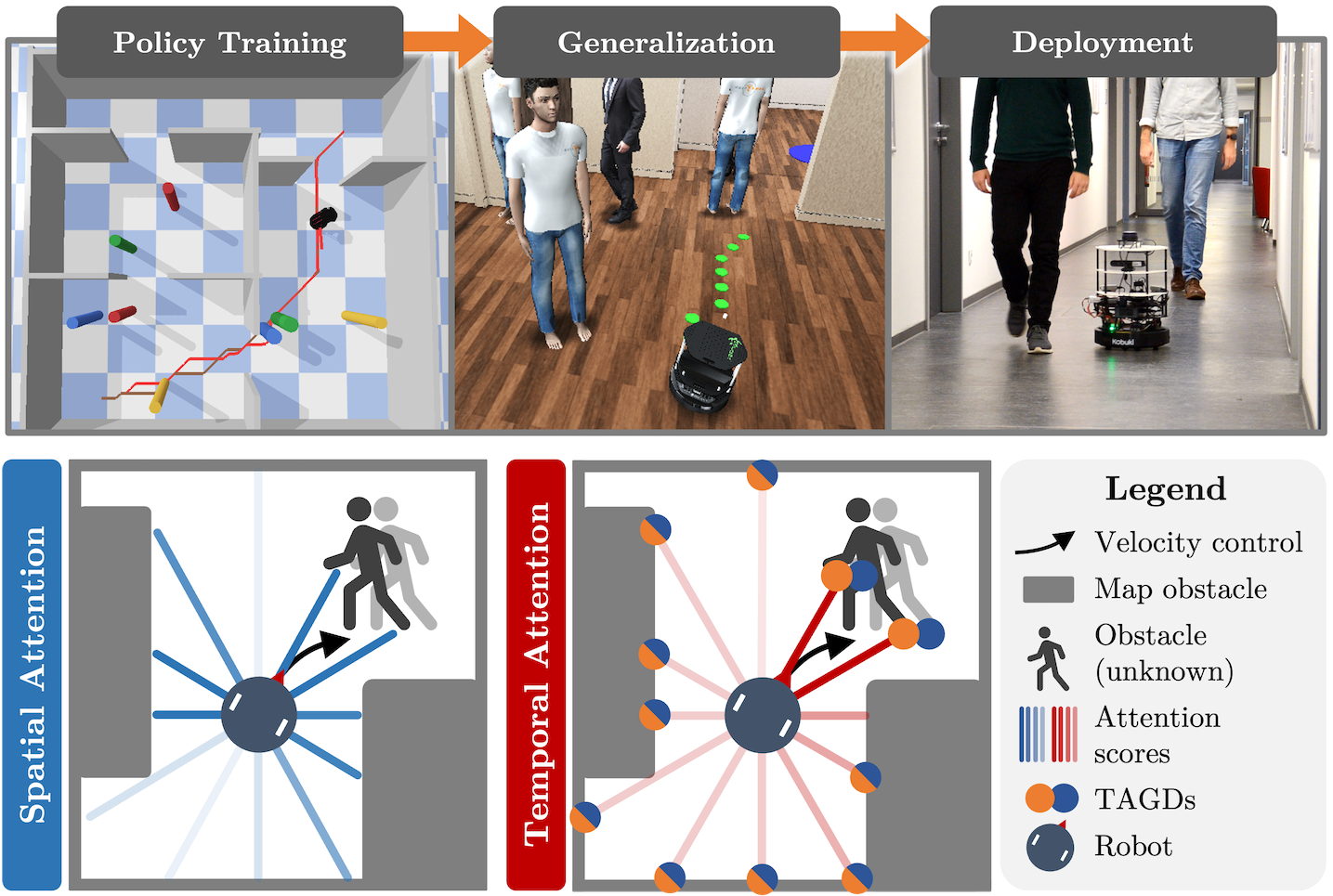
Figure 1: Our pipeline for learning a robot navigation controller based on lidar. Two attention mechanism reason about the importance of individual lidar sectors with respect to known and unknown dynamic obstacles. Our Temporal Accumulation Group Descriptors (TAGD) reveal moving obstacles from subsequent lidar scans affected by robot self-motion.

An appealing idea to tackle these sensor-implicit obstacle representations is selective attention on a collision-relevant sub-sectors of the lidar data [18]. Especially when a temporal observation sequence provides dynamic scene information, selective attention on moving obstacles can be beneficial.

To address the issues above, we introduce a lightweight 2D lidar-based reinforcement learning setup incorporating both spatial and temporal attention across the sensor readings. It allows the robot to navigate smoothly and safely in dynamic, cluttered environments, by outputting continuous velocity commands. Our minimalistic indoor training environments foster good generalization to unseen navigation scenarios and enable a smooth sim-to-real transfer of the learned policy, as we will be able to demonstrate in the experiments.

In summary, the main contributions of our work are:

• A deep reinforcement learning-based (DRL) navigation controller that learns dynamic obstacle avoidance implicitly from 2D lidar readings only.

• A spatiotemporal attention module that infers the relative importance of different observation sectors with respect to proximity and obstacle motion trends.

• A novel observation representation highlighting dynamic obstacles over the robot’s self-motion called temporal accumulation group descriptor (TAGD).

II Related Work

Mobile robot navigation can be tackled with traditional and learning-based approaches, as highlighted in the following.

II-A Traditional Navigation

Generally, robot navigation can be roughly divided into global and local path planning according to the known degree of the environment information. Traditional global path planning computes a path on a known map. Commonly used methods are the A* algorithm [19], or the Rapidly-Exploring Random Tree algorithm [20]. They suffice in static and fully-mapped environments, but fail with dynamic and unknown obstacles. Here, local path planning algorithms come for rescue [21]. One example is the widely used dynamic window approach (DWA) [22, 23], but with the drawback of DWA’s difficulties to avoid C-shaped or dynamic obstacles. While unable to explicitly account for dynamic obstacles in its original formulation, DWA has been advanced with motion prediction [24].

A well-tuned DWA offers decent performance but needs re-tuning for different environments [25]. For collision avoidance among multiple independent agents, Optimal Reciprocal Collision Avoidance (ORCA) algorithm [26] provides a feasible solution. However, known speeds of surrounding agents are an inconvenient requirement.

In our paper, we make use of a traditional global planner for high-level guidance to the robot on its way to a global goal. Our contribution however focuses on the local planning, which we replace with a learning-based obstacle avoidance policy.

II-B Learning-based navigation

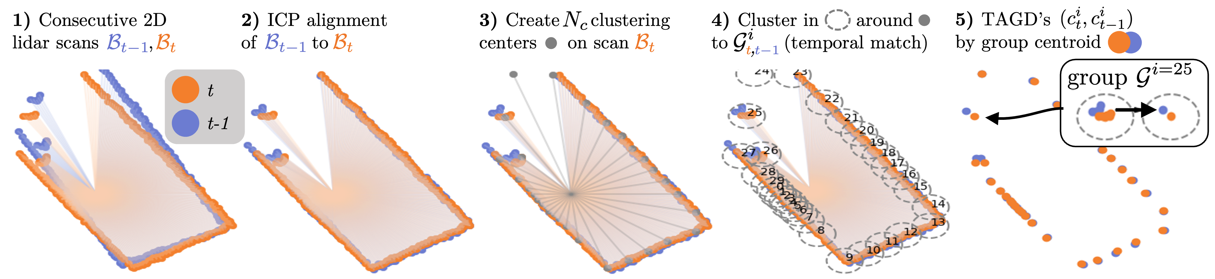
Figure 2: Schematic of the TAGD generation process. The ICP alignment of two subsequent lidar scans (1) in 2D Cartesian coordinates reduces the effect of robot self-movement (2). This allows better differentiation between dynamic obstacles and static obstacles. The aligned scan is grouped and clustered around ray-casted centers (3). From the clustered points (4), the position difference of the centroid from both time steps reveals a moving obstacle (5).

Deep learning-based methods [27, 28, 29, 30] are widely used in the field of mobile robot navigation. They appeal with decent generalization performance and less tedious fine-tuning as compared to hard-coded controllers.

Especially reinforcement learning-based (RL) methods have recently been applied to motion planning [31, 13, 32, 33, 18]. Due to their reward structure, they are mostly suited for short-distance navigation, while struggling with long-distance navigation during training[30]. Hence, the employment of RL controllers for local collision avoidance lies at hand [34, 35, 18].

These works however do not embed dynamic scene understanding, thus limiting the agent’s capability around walking pedestrians. Methods like SARL [36] or MP-RGL [37] capture interactions between robot and humans with excellent results, but rely on the known velocity of humans. Others infer or forecast human behavior by predicting their long-term goals, or by predicting their future motion and activities [38], often by employing 3D lidar or RGB(D) cameras [39, 40, 41, 42, 43]. Wang et al. [44] processed optical flow from RGB data as temporal information with an attention module to detect actions. Liang et al. [43] used a 2D lidar alongside a depth camera to perceive surrounding dynamic pedestrians and compute collision-free velocities. The challenge arises with our aim to learn time-series motion trends for scene-dynamics aware navigation from 2D lidar readings in an end-to-end manner.

III Problem Statement and Assumptions

In this work, we consider a differential-wheeled robot pursuing a global goal in a cluttered and dynamic indoor environment, compare Fig. 3a). A map of the empty environment is available for global path planning via A*. Static or dynamic pedestrians however are unknown obstacles to the robot. Also, the pedestrians at different speeds move rigorously without avoiding the robot in their motion, in contrast to other social navigation studies [45]. Therefore, smart and foresighted local collision avoidance is entirely up to the robot. The controlling agent has access to subsequent 2D lidar readings and upcoming path waypoints as observations, which it maps to linear and angular velocity commands. We formulate the task as in a learning-based manner and apply off-policy DRL. In summary, the proposed controller should be able to achieve two tasks: 1) Pursue the global goal through guidance of the computed path and 2) effectively avoid dynamic obstacles on a local scale.

IV Our Approach

This section explains our novel temporal accumulation group descriptor for lidar readings and subsequently the learning framework.

IV-A Temporal Accumulation Group Descriptor (TAGD)

It is inherently difficult to capture motion trends of moving obstacles from consecutive 2D lidar readings when the robot is in motion. To deal with that problem, we introduce our novel Temporal Accumulation Group Descriptor (TAGD).

Using Iterative Closest Points (ICP) [46], we firstly align the previous sensor reading to the current reading. In other words, the ego-centric perspective of the previous lidar reading is shifted to the current robot location. With a temporal matching procedure, moving obstacles become distinguishable from static obstacles. Our approach works as follows:

1) Generate a uniformly distributed subset of $N$ 2D lidar points via min-pooling. Their positions are collected in sets for the previous and current time step, represented as $\mathcal{B}_{t-1}=\{\mathbf{b}^{i}_{t-1}|0\leq i<N\}$ and $\mathcal{B}_{t}=\{\mathbf{b}^{i}_{t}|0\leq i<N\}$. Here, $\mathbf{b}^{i}_{t}=[x^{i}_{t},y^{i}_{t}]$ is the 2D end position of the $i$-th beam.

2) Align $\mathcal{B}_{t-1}$ to $\mathcal{B}_{t}$ via ICP [47], which eliminates the impact of robot rotation and translation. For static obstacles, the points now match up while their positions misalign for dynamic obstacles. The transformed point set is represented as $\mathcal{B}^{{}^{\prime}}_{t-1}$.

3) Cast $N_{c}$ circular-uniformly spaced rays from the robot origin to the points of set $\mathcal{B}_{t}$ at time step $t$, while slightly inflating the points to circles in the 2D plane to create surfaces for ray-casting. Upon ray impact, the original 2D position of the point provides the center for a clustering group $\mathcal{G}^{i}$, where $i\in\{1,\dots,N^{c}\}$.

4) For temporal matching, assign the points in sets $\mathcal{B}^{{}^{\prime}}_{t-1}$ and $\mathcal{B}_{t}$ to the clustering groups $\mathcal{G}^{i}_{t-1}$ and $\mathcal{G}^{i}_{t}$ based on Euclidean distance within a threshold $d_{thresh}$.

5) Calculate the 2D centroids $\mathbf{c}_{t}^{i}=\{x_{t}^{i},y_{t}^{i}\}$, $\mathbf{c}_{t-1}^{i}=\{x_{t-1}^{i},y_{t-1}^{i}\}$ for each group $\mathcal{G}^{i}_{t-1}$ and $\mathcal{G}^{i}_{t}$. This counteracts sensor noise, the impact of robot displacement and turning, and also ICP matching inaccuracy. Those centroids of two time steps represent a single TAGD $(\mathbf{c}_{t}^{i},\mathbf{c}_{t-1}^{i})$.

A visualization of all steps is shown in Fig. 2. A TAGD represents the center of the data points across two consecutive lidar scans within a certain region. Note that it is possible for a single dynamic obstacle to be represented in more than one TAGD, depending on the positions of clustering centroids, e.g., see TAGDs 26 and 27 in Fig. 2.4). However, such double representations did not hinder the performance in context of the learned controller. In summary, TAGDs reveal obstacle motion and will therefore be used as input to the temporal attention module of our pipeline.

IV-B Deep Reinforcement Learning for Navigation

We choose a deep deterministic policy gradient (DDPG) architecture consisting of an actor and a critic, modeled by neural networks [48]. DDPG features a continuous action space, allowing for smooth robot control. The actor network outputs linear and angular velocities for the robot. The RL framework is based on the Markov Decision Process: An agent in state $s_{t}$ at time step $t$ decides upon an action $a_{t}$ based on a policy $\pi(s_{t})=a_{t}$. Upon reaching the next state $s_{t+1}$, it receives a reward $r_{t}$. The optimization objective is the maximization of the $\gamma$-discounted cumulative return $R=\sum_{i=t}^{T}\gamma^{i-t}r_{t}$, where $\gamma=0.98$ As DDPG is an off-policy RL algorithm, the state-action pairs are stored in a experience replay buffer of length $N_{\text{RP}}=50,000$ and sampled in batches for policy updates.

IV-C State and Action Space

The state space defines the observations we provide to the agent. As can be seen in Fig. 3b, the agent has access to 2D lidar sensor data, the lidar-derived TAGDs, and upcoming waypoints for global guidance:

• The lidar scan is represented as a set of robot-centric Cartesian 2D points as $\mathcal{B}_{t}$. As we only aim to avoid local dynamic obstacles with our controller, the beam’s maximum scanning range is limited to $d_{max}=$3.5$$\mathrm{m}$$. During spatial attention processing, the set of $N=180$ rays will be split into $N_{b}=30$ circular-spaced sectors.

• The TAGDs for time step $t-1$ and $t$ are grouped as $\mathcal{C}_{t}=\{\mathbf{c}_{t}^{i},\mathbf{c}_{t-1}^{i}|0\leq i<N_{c}\}$, as described in the section above, where the number of TAGD’s $N_{c}=30$ is equal to the number of spatial sectors $N_{b}$.

• Path waypoints: Assume that the robot is closest to waypoint $\mathbf{p}^{c}$ on the initially planned path $\mathcal{P}$. From here, we sample $N_{f}=5$ equidistant waypoints $\Delta\mathbf{p}^{i}=$0.3$$\mathrm{m}$$ into the goal direction and provide them as input to the agent as $\mathcal{P}_{t}^{f}=\{\mathbf{p}^{i}|c\leq i<c+N_{f}\}$.

The continuous action space of the agent consists of linear and angular velocities $(v,w)$, with a range of $v\in[0,0.5]$\mathrm{m}\text{\,}{\mathrm{s}}^{-1}$$ and $w\in[-\pi,\pi]$\mathrm{rad}\text{\,}{\mathrm{s}}^{-1}$$. The robot is not allowed to drive backwards to foster foresighted navigation.

IV-D Reward

The overall objective of the navigating agent is collision-free navigation along a given path with unknown dynamic obstacles. The reward $r_{t}$ is therefore a weighted sum:

$$r_{t}=\alpha_{1}r^{\text{collision}}_{t}+\alpha_{2}r^{\text{guide}}_{t}+\alpha_{3}r^{\text{proximity}}_{t}$$ (1)

$\alpha_{1}=10$, $\alpha_{2}=0.3$ and $\alpha_{3}=3$ are the weighting factors.

To encourage collision-free navigation, we penalize with $r^{\text{collision}}=-1$ upon collision of the robot with any obstacles.

A natural guidance along the global path is beneficial as it encourages the agent to drive towards the goal. From the current closest waypoint $\mathbf{p}^{c}$ on the path to the robot, we interpolate $0.6$\mathrm{m}$$ forward along the path to obtain the guidance point $\mathbf{p}^{g}$. The distance between $\mathbf{p}^{g}$ and the robot’s position $\mathbf{p}^{r}$ are penalized with $r^{\text{guide}}=-||\mathbf{p}^{g}-\mathbf{p}^{r}||$. By design and due to the update at every time step, $\mathbf{p}^{g}$ cannot be reached, thus providing a continuous penalty that increases when the robot deviates from the path. Upon deviation, it encourages the robot to drive back to the path in a forward-leading manner.

The concept of $r^{\text{proximity}}$ aligns with the sparse collision reward, but does not terminate the episode for easier learning. Instead it alerts the agent in vicinity to obstacles about higher risk of collisions, or in other words encourages the agent to keep clear of obstacles. When the minimum distance $d$ between robot and any lidar-scanned obstacle falls below a threshold $d_{\text{proximity}}$, a linearly growing penalty is computed as $r^{\text{proximity}}=-1\times|d_{\text{proximity}}-\min(d,d_{\text{proximity}})|$, else $r^{\text{proximity}}=0$.

IV-E Network Architecture

As shown in Fig. 3c, our agent’s architecture is constructed around two data streams. The individual streams extract spatial and temporal features via an attention mechanism, respectively. Note that both the down-sampled lidar input of the spatial, and the TAGD input of the temporal steam contain partially redundant information due to their origin in the raw distance readings.

IV-E1 Temporal and Spatial Data Stream

In the temporal data stream, the data of two consecutive time steps is processed. We construct $N_{c}=30$ individual vectors by concatenating both time step’s two-dimensional TAGDs $\mathbf{c}_{t-1}^{i}$ and $\mathbf{c}_{t}^{i}$ with the next path segment set $\mathcal{P}^{f}_{t}$. Note the redundant representation of $\mathcal{P}^{f}_{t}$ in all $N_{c}$ vectors, since the importance of individual TAGDs can depend on the future path segment. Those individual vectors are then passed on the temporal attention module, see Fig. 3e.

In the spatial data stream, we feed lidar readings of higher resolution as compared to the single position TAGD. Firstly, the lidar scan of $N=180$ rays at time step $t$ is split into $N_{b}=30$ sectors with $N/N_{b}$ rays each. Again, each sector-vector is concatenated with next path segment set $\mathcal{P}^{f}_{t}$. Those $N_{b}$ individual vectors are then passed on to the spatial attention module.

After both data streams have been processed by their attention modules, respectively, they are concatenated and jointly processed by an output module. From here, the data is passed to the actor and critic networks of DDPG.

IV-E2 Attention module

Both temporal and spatial attention modules share a similar network architecture, but no parameters. A visualization of our lightweight attention module can be found in Fig. 3d-e. It is constructed with an embedding, a score and a feature network, inspired by Chen et al. [36] and [18]. The embedding module encodes the input vectors individually along the attention dimension. The embedding is fed into the score module that outputs the attention score of each input vector $i$. All attention scores are Softmax-normalized to obtain the final importance weight. In parallel the embedding is also fed into the feature module that generates the feature representations of each embedding vector $i$. Finally, the feature vectors are scaled by their importance in a weighted sum. Note that the due to the lightweight implementation of our attention scheme, the dimensionality along the attention axis has been reduced from $N_{b}$ or $N_{c}$ vectors to one in the output. In other words, the individual embedded lidar sectors or TAGDs do not attend to each other, but the attention scales their impact in the weighted sum, respectively. This form of attention is also referred to as location-based attention [49, 50]. All networks describe above are constructed with as ReLU-activated multi-layer perceptrons (MLP).

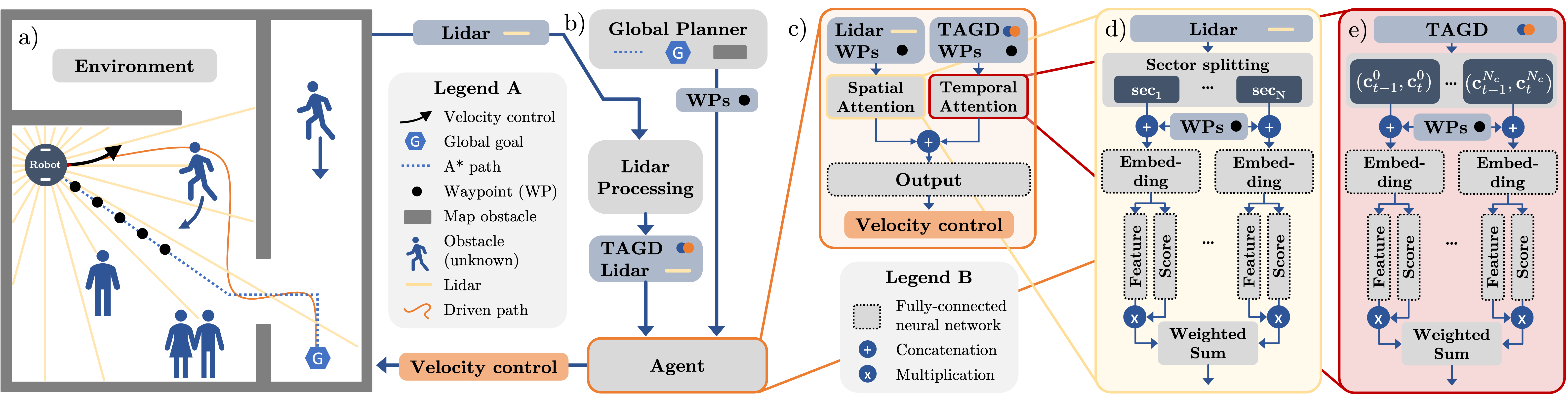
Figure 3: Illustration of our architecture. a) The indoor environment provides lidar readings to the deep reinforcement learning agent that drives a differential-wheeled robot via linear and angular velocity commands. b) From subsequent lidar readings, the TAGDs are computed. Merged with the five upcoming waypoints of the global path and the raw lidar readings as observations, they are c) processed by the agent in a separate spatial and temporal stream. Both streams feature an attention block to weigh the importance of d) individual lidar sectors (spatial) or e) the TAGDs (temporal), with respect to the upcoming waypoints. After feature extraction, both streams are concatenated for further processing in the final output network of the actor-critic agent.

IV-F Indoor Training Environments and Pedestrians

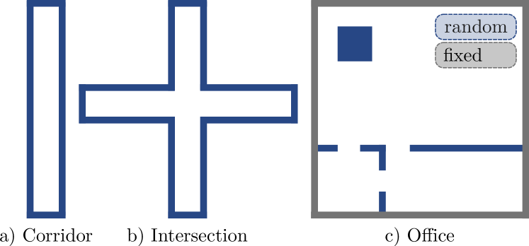
Figure 4: The Pybullet-based environments of [18] are used for training. a) In the corridor and b) intersection environment, the wall distances are randomized (blue). c) In the office environment, the outer walls are fixed with randomized inner wall placement for diverse room setups.

To train our navigation agent, we use the Pybullet[51] physics engine. We use the minimalistic but well-randomizing environments of de Heuvel et al. [18] with three different types of scenarios, see Fig. 4: Corridors, intersections, and offices. The randomization of wall density and placement determines provides varying levels of environment complexity. Dynamic and static pedestrians represented by cuboids move through the environments along A* paths with randomized speed, start, and goal position.

The corridor environment is long and narrow with a length between $[6$\mathrm{m}$,8$\mathrm{m}$]$ and a width between $[2.0$\mathrm{m}$,2.5$\mathrm{m}$]$. The robot encounters pedestrians with opposite directions.

The intersection environment is cross-shape with a short edge and a long edge. The hallway width falls in the range of $[2.0$\mathrm{m}$,2.5$\mathrm{m}$]$. The corners provide blind spots, from which pedestrians may suddenly appear.

The office environment has a fixed outer size and randomized interconnected rooms. A novelty over the other environments are the doorway encounters between robot and pedestrian, where the robot needs to wait for clearance of the pedestrian before continuing.

The robot’s start and goal location are sampled in the corners or dead ends of the environments, respectively. For the purpose of increasing the obstacle encounter likelihood with the robot, start and goal locations of some pedestrians are sampled around the robot path. Note that the A*-following pedestrians do not take into account each other or the robot position, but rigorously move forward. Collision avoidance is therefore entirely up to the robot.

IV-G Robot Model

We employ a differential-wheeled robot, more precisely, the Kobuki Turtlebot 2. The Turtlebot performs angular turns with a speed difference between both wheels. A Slamtec RPlidar A3 2D lidar sensor is mounted on top of the Turtlebot, emitting 1,440 beams. In simulation, we artificially add sensor noise to the distance readings with an amplitude of $2.5$$\mathrm{cm}$.

V Experiments

In the following we present the training and evaluation details, followed by an ablation and baseline study. After evaluating the domain shift to the iGibson simulator, the section is rounded up by the real-robot deployment.

V-A Training Setup

An episode denotes one navigation run of the robot from start until one of the termination criteria is reached: Collision with other obstacles, timeout after $T_{\text{timeout}}=150\equiv 60$\mathrm{s}$$ steps, or goal-reaching upon vicinity of $0.2$\mathrm{m}$$ to the global goal. To foster generalization abilities, for each episode a randomly generated environment is setup, as described in Sec.IV-F. The inference and control time step of the agent set to $0.4$$\mathrm{s}$, which also represents the time difference between subsequent lidar scans for the temporal processing. The initial learning rate $l=$1\text{\times}{10}^{-4}$$ is gradually decayed over the course of training to $l=$1\text{\times}{10}^{-6}$$. All agents presented are trained for 100,000 episodes, and evaluated regularly. After training, the best performing model checkpoint is selected for all approaches, respectively.

V-B Quantitative Performance

Figure 5: Performance overview for all approaches averaged over 1,000 episodes with identical scene setups in all three Pybullet environments for a) increasing obstacle speeds, with two dynamic and one static pedestrians, and b) increasing number of obstacles, with a fixed pedestrian speed $0.3$\mathrm{m}\text{\,}{\mathrm{s}}^{-1}$$. The superiority of attention-based lidar processing (OUR-A3, B4) over the baseline CNN approaches (B1-3) can be observed, as well as a decline in performance with increasing scenario complexity. Note the y-axis intercept at $50$\mathrm{\char 37\relax}$$.

We evaluated our trained models with respect to success rate, collision rate, timeout rate, and navigation time over 1,000 episodes. For comparability, the 1,000 episodes were setup identically among all approaches. The flagship approach presented in this study is denoted with OUR. Generally, with challenging environment complexity due to increased obstacle velocities (Fig. 5a), or increased number of dynamic obstacles (Fig. 5b), the success rate stagnates.

Figure 6: Exemplary visualization of the a) spatial (blue) and b) temporal attention (red) for a given navigation scene. The attention scores were color-mapped onto the lidar beam sectors for the spatial and on the beams pointing towards the TAGDs for the temporal attention, respectively. Increased spatial attention towards the forward-facing lidar sectors, as well as increased temporal attention towards the oncoming dynamic obstacle can be observed.

V-B1 Ablation Study

We did an ablation study with respect to OUR approach described above to evaluate the contribution of each module to the results, see Tab. Ia) and Fig. 5.

A1 NO-SPATIAL: As OUR, but removing the spatial attention stream, leaving only TAGD and waypoint processing.

A2 NO-TEMPORAL: As OUR, but with no temporal stream or TAGD input, leaving only the spatial single time step attention stream and waypoint processing.

A3 NO-TAGD: As OUR, but without TAGD preprocessing. The network structure implements the spatial attention stream twice with separate network parameters, each processing one of the consecutive lidar scans, respectively.

As can be seen from Tab. Ia) and Fig. 5, with all ablations the performance deteriorates, while A1 NO-SPATIAL that processes only TAGDs on the temporal stream comes closest to OUR’s. The isolated TAGD temporal stream also seems beneficial for higher obstacle numbers. The all spatial-approach A2 NO-TEMPORAL deteriorates stronger for increasing obstacle velocities as compared to approaches with temporal attention, as expected.

a)	Ablation	SR$\uparrow$	CR$\downarrow$	TR$\downarrow$	Nav. time$\downarrow$
	OUR	96.0	4.0	0.0	17.8 $\mathrm{s}$
	A1: NO-SPATIAL	94.5	5.5	0.0	17.6 $\mathrm{s}$
	A2: NO-TEMPORAL	92.7	7.3	0.0	17.7 $\mathrm{s}$
	A3: NO-TAGD	91.6	8.4	0.0	17.5 $\mathrm{s}$
b)	Baseline
	B1: Liang et al. [43]	85.5	14.5	0.0	17.2 $\mathrm{s}$
	B2: Pérez-D. et al. [45]	88.2	11.6	0.2	18.3 $\mathrm{s}$
	B3: Pérez-D. et al. [45]	87.4	12.5	0.1	17.9 $\mathrm{s}$
	B4: de Heuvel et al. [18]	90.7	9.3	0.0	19.5 $\mathrm{s}$
c)	Generalization
	iGibson [52]	63.7	10.6	25.7	15.6 $\mathrm{s}$

TABLE I: Performance rates in [$\mathrm{\char 37\relax}$] with respect to success (SR), collision (CR), and timeout (TR) and average navigation times for successful episodes of a) ablation and b) baseline study averaged over 1,000 episodes, with $2$ dynamic pedestrians ($0.3$\mathrm{m}\text{\,}{\mathrm{s}}^{-1}$$) and $1$ static pedestrian. The c) generalization evaluation reveals slightly decreased performance for the post-training domain shift to the iGibson simulator on similar navigation tasks in more complex environments.

V-C Baselines

To identify the contribution of our approach, we compared against three baseline architectures. All baselines leverage 2D lidar ($360$$\mathrm{\SIUnitSymbolDegree}$) for learning-based mobile robot navigation and were trained in the same environment as our approach. Except for the last baseline (de Heuvel et al. [18]), the training setup of our approach with regards to action space, reward, and RL implementation was used. The baseline-related modifications lie in the content of the state space and the processing network architectures.

V-C1 Liang et al. - B1

A highly-related state-of-the-art approach has been presented in [43]. Similarly to ours, it is an end-to-end obstacle avoidance algorithm originally trained with Proximal Policy Optimization (PPO). The authors use 2D lidar and a depth camera to perceive the environment, while the controller outputs velocity commands. From both perception modalities, we solely implement the lidar-related preprocessing and network architecture to replace our attention blocks, which is a 1D convolutional neural network (CNN) taking in three consecutive scans. Precisely, this module is composed of two 1D CNN layers followed by a fully-connected MLP. In contrast to our approach with 2D Cartesian point lidar representation, single-value lidar distance readings at the same resolution are used. The state space still contains five upcoming waypoints, which in contrast to OUR are processed by a separate MLP. Unsuccessfully without convergence and therefore not included, we have also tested a closer-to-the-original state space implementation (512 lidar readings, no path waypoints, but with final goal position).

V-C2 Pérez-D’Arpino et al. - B2/3

In the end-to-end lidar navigation approach of [45], no temporal information but only the current lidar reading is processed. Similar to Liang et al. [43], the authors employ a lidar-processing 1D CNN but with three layers followed by a fully-connected layer. Furthermore, $N=$128$$ single-value lidar distance readings are used. Additionally, the global goal position and next upcoming waypoints of the A* path ($\Delta\mathbf{p}^{i}=$1.0$$\mathrm{m}$$) are part of their state space. In B2, we employ their state space and replace our attention block with their lidar-processing CNN and waypoint-processing MLP architecture. A sub-version (B3) of this baseline uses only their CNN architecture but our original state space with regards to waypoints and lidar resolution.

V-C3 de Heuvel et al. - B4

This baseline [18] features a different output modality - subgoals instead of velocity commands. For dynamic obstacle avoidance, the subgoals are placed in the vicinity of the robot by a high-level agent and pursued by a low-level controller. Similarly to this study, an attention module processes the spatial importance of single-time step lidar readings, but no temporal information from subsequent scans. Note that we employ the same training environments, allowing for a direct comparison of results. The original inference time step of $0.2$\mathrm{s}$$ and reward setup for the high-level subgoal agent has been used.

As can be seen in Tab. Ib) and Fig. 5, for our setup, the CNN-related baselines B1-B3 struggle with increased number of obstacles. The subgoal-placing baseline B4 is the most compelling rival, especially among higher numbers of obstacles. In summary, our approach outperforms all baselines in terms of success rate.

V-D Qualitative Attention Analysis

Fig. 6 visualizes the learned spatial (a) and temporal (b) attention for a given navigation scenario. Here, two dynamic obstacles approach the robot from opposite directions, the robot has just entered the room. The spatial attention highlights the forward lidar sectors in the desired direction of navigation. The robot navigates along a wall that locates on its left hand side and we can observe an increased attention on the corresponding lidar sectors. Intuitive to the human eye, the temporal attention focuses the TAGDs of the oncoming dynamic obstacles. Similar to the spatial attention, a slightly increased temporal attention can be observed in forward direction of the robot. In direct comparison to the temporal stream, the spatial stream exhibits a less sharp attention distribution in this scenario. Further attention visualizations can be found in the accompanying video.

V-E Generalization Performance

Figure 7: Results of the generalization study using the iGibson simulator over eight scenes witch $125$ episodes each. a) The different approaches exhibit more timeout events in iGibson as compared to the Pybullet environments, which results in a lower success rate. Our controller reveals the least number of collisions in iGibson and rather gets stuck than colliding. b) Breakdown into the different scenes shows a scene-dependency of the controller performance for OUR controller. c) Collision object category analysis within iGibson: The most collided-with objects are the walls, followed by tables and chairs.

To investigate the generalization ability of our approach, we evaluated the Pybullet-trained agents in the iGibson simulator [52] in a sim-to-sim transfer, see Fig. 1. The sensor settings and overall navigation objective remain similar, but two major differences strike: 1) The indoor scenarios are of high fidelity with diverse furniture objects and a more complex room architecture. 2) The pedestrians are represented with real 3D meshes instead of cuboids and have a more refined motion simulation. Precisely, we adapt the navigation task from the 2021 iGibson Social Navigation Challenge [53] that features eight scenes and Optimal Reciprocal Collision Avoidance (ORCA) among pedestrians. The key settings to mention as taken over from the original challenge are the maximum pedestrian speed of $0.5$\mathrm{m}\text{\,}{\mathrm{s}}^{-1}$$, an inverse scene area-related population of 8 ${\mathrm{m}}^{2}$ per pedestrian, and a goal sample distance between 1.0 and $10.0$\mathrm{m}$$.

As seen in Fig. 7a), OUR controller exhibits the smallest collision rate. The lower success rates in Fig. 7a) and Tab. Ic) point towards a simulator gap and increased difficulty within the scenes. Compared to the Pybullet evaluation, the noticeably higher timeout rates indicates a generally conservative navigation behavior in impassable and confined situations. Also, the individual scenes seem to be of varying difficulty to the robot, compare Fig. 7b). To further differentiate the challenges the robot faces in the iGibson scenes, the top ten collided-with object categories have been recorded, see Fig. 7c). As the majority of collisions events involve walls, the possibly higher degree of confined spaces within the iGibson scene could play a role. Furthermore, tables and chairs are the next most frequent collision causes. These object are usually thin-legged, providing a challenge for lidar detection at low angular resolutions. Comparatively few collisions with pedestrians have been recorded, which points towards careful navigation around pedestrians, as encouraged by the proximity reward during training.

V-F Real-World Experiment

Using the Robot Operating System (ROS)[54], we transferred the trained controller to a real Kobuki Turtlebot 2, as described in Sec. IV-G. In our experiment, the Gmapping package [55], a Simultaneous Localization and Mapping algorithm, was used to build an occupancy grid map of real scenarios upfront for path planning. During navigation, we applied Adaptive Monte Carlo Localization (AMCL) [56] to estimate the robot’s pose in the pre-mapped environment based on the lidar reading and robot odometry.

We tested our learning-based spatiotemporal approach qualitatively in various real-world scenarios, including corridors, intersections, and offices. Please refer to our supplemental video2 of the real-world experiment. In a corridor, the two participants overtake the robot from behind or approach it rigorously from the front, see Fig. 1. The robot smoothly gives room to the pedestrians and avoids collision. At an intersection, pedestrians appear from the blind spots behind a corner. In another test the pedestrian blocks the doorway to see whether the robot would stop upon facing the impassable situation. All navigation situations are successfully handled our spatiotemporal controller.

VI Conclusions

We proposed a novel and lightweight approach for robot navigation in dynamic indoor environments. Our learning-based approach featuring spatiotemporal attention demonstrates the capacity to highlight collision-relevant features from the sensor data, making the most out of the sparse 2D-lidar readings. Meanwhile, the introduced temporal accumulation group descriptors (TAGD) help to counteract the robot self-movement over subsequent lidar readings and therefore support the differentiation between static and dynamic obstacles without explicit object tracking. Our policy directly outputs linear and angular velocity, leading to smooth robot navigation, and outperforms several state-of-the-art approaches in terms of collision rate for different pedestrian speed and number of obstacles. We validate the sim-to-sim generalization capabilities in the iGibson simulator, finding conservative navigation behavior in the more confined spaces. Lastly, we achieve an effortless sim-to-real transfer into dynamic real-world indoor environments.

References

- [1] S.-Y. Chung and H.-P. Huang, “Predictive navigation by understanding human motion patterns,” International Journal of Advanced Robotic Systems, vol. 8, no. 1, 2011.
- [2] N. Sakata, Y. Kinoshita, and Y. Kato, “Predicting a pedestrian trajectory using seq2seq for mobile robot navigation,” in IECON 2018-44th Annual Conference of the IEEE Industrial Electronics Society. IEEE, 2018.
- [3] K. D. Katyal, G. D. Hager, and C.-M. Huang, “Intent-aware pedestrian prediction for adaptive crowd navigation,” in Proc. of the IEEE Intl. Conf. on Robotics & Automation (ICRA). IEEE, 2020.
- [4] A. Wang, C. Mavrogiannis, and A. Steinfeld, “Group-based motion prediction for navigation in crowded environments,” in Conference on Robot Learning. PMLR, 2022.
- [5] Y. Wang, Q. Mao, H. Zhu, J. Deng, Y. Zhang, J. Ji, H. Li, and Y. Zhang, “Multi-modal 3d object detection in autonomous driving: a survey,” International Journal of Computer Vision, 2023.
- [6] C. Wang, C. Ma, M. Zhu, and X. Yang, “Pointaugmenting: Cross-modal augmentation for 3d object detection,” in Proc. of the IEEE Conf. on Computer Vision and Pattern Recognition (CVPR), 2021.
- [7] H. Surmann, C. Jestel, R. Marchel, F. Musberg, H. Elhadj, and M. Ardani, “Deep reinforcement learning for real autonomous mobile robot navigation in indoor environments,” arXiv preprint arXiv:2005.13857, 2020.
- [8] M. Stefanczyk, K. Banachowicz, M. Walecki, and T. Winiarski, “3d camera and lidar utilization for mobile robot navigation,” Journal of Automation, Mobile Robotics and Intelligent Systems, 2013.
- [9] J. Li, H. Qin, J. Wang, and J. Li, “Openstreetmap-based autonomous navigation for the four wheel-legged robot via 3d-lidar and ccd camera,” IEEE Transactions on Industrial Electronics, vol. 69, no. 3, 2021.
- [10] M. Himmelsbach, F. V. Hundelshausen, and H.-J. Wuensche, “Fast segmentation of 3d point clouds for ground vehicles,” in 2010 IEEE Intelligent Vehicles Symposium. IEEE, 2010.
- [11] G. Csaba, L. Somlyai, and Z. Vámossy, “Mobil robot navigation using 2d lidar,” in 2018 IEEE 16th world symposium on applied machine intelligence and informatics (SAMI). IEEE, 2018.
- [12] H. Beomsoo, A. A. Ravankar, and T. Emaru, “Mobile robot navigation based on deep reinforcement learning with 2d-lidar sensor using stochastic approach,” in 2021 IEEE International Conference on Intelligence and Safety for Robotics (ISR). IEEE, 2021.
- [13] L. Tai, G. Paolo, and M. Liu, “Virtual-to-real deep reinforcement learning: Continuous control of mobile robots for mapless navigation,” in Proc. of the IEEE/RSJ Intl. Conf. on Intelligent Robots and Systems (IROS). IEEE, 2017.
- [14] E. Salvato, G. Fenu, E. Medvet, and F. A. Pellegrino, “Crossing the Reality Gap: A Survey on Sim-to-Real Transferability of Robot Controllers in Reinforcement Learning,” IEEE Access, vol. 9, 2021.
- [15] X. Chen, J. Hu, C. Jin, L. Li, and L. Wang, “Understanding Domain Randomization For Sim-To-Real Transfer,” in 10th International Conference on Learning Representations, ICLR 2022, 2022.
- [16] B. Qin, Z. J. Chong, S. H. Soh, T. Bandyopadhyay, M. H. Ang, E. Frazzoli, and D. Rus, “A spatial-temporal approach for moving object recognition with 2d lidar,” in Experimental Robotics: The 14th International Symposium on Experimental Robotics. Springer, 2016.
- [17] Y. Song, Y. Tian, G. Wang, and M. Li, “2d lidar map prediction via estimating motion flow with gru,” in Proc. of the IEEE Intl. Conf. on Robotics & Automation (ICRA). IEEE, 2019.
- [18] J. de Heuvel, W. Shi, X. Zeng, and M. Bennewitz, “Subgoal-Driven Navigation in Dynamic Environments Using Attention-Based Deep Reinforcement Learning,” arXiv preprint arXiv:2303.01443, Mar. 2023.
- [19] P. E. Hart, N. J. Nilsson, and B. Raphael, “A formal basis for the heuristic determination of minimum cost paths,” IEEE transactions on Systems Science and Cybernetics, vol. 4, no. 2, 1968.
- [20] S. Karaman and E. Frazzoli, “Sampling-based algorithms for optimal motion planning,” The international journal of robotics research, vol. 30, no. 7, 2011.
- [21] M. Missura, A. Roychoudhury, and M. Bennewitz, “Fast-Replanning Motion Control for Non-Holonomic Vehicles with Aborting A*,” in Proc. of the IEEE/RSJ Intl. Conf. on Intelligent Robots and Systems (IROS), Oct. 2022.
- [22] D. Fox, W. Burgard, and S. Thrun, “The dynamic window approach to collision avoidance,” IEEE Robotics & Automation Magazine, vol. 4, no. 1, 1997.
- [23] O. Brock and O. Khatib, “High-speed navigation using the global dynamic window approach,” in Proc. of the IEEE Intl. Conf. on Robotics & Automation (ICRA), vol. 1. IEEE, 1999.
- [24] M. Missura and M. Bennewitz, “Predictive Collision Avoidance for the Dynamic Window Approach,” in Proc. of the IEEE Intl. Conf. on Robotics & Automation (ICRA), May 2019.
- [25] X. Xiao, B. Liu, G. Warnell, J. Fink, and P. Stone, “Appld: Adaptive planner parameter learning from demonstration,” IEEE Robotics and Automation Letters (RA-L), vol. 5, no. 3, 2020.
- [26] J. Alonso-Mora, A. Breitenmoser, M. Rufli, P. Beardsley, and R. Siegwart, “Optimal reciprocal collision avoidance for multiple non-holonomic robots,” in Distributed autonomous robotic systems. Springer, 2013.
- [27] F. Shamsfakhr and B. S. Bigham, “A neural network approach to navigation of a mobile robot and obstacle avoidance in dynamic and unknown environments,” Turkish Journal of Electrical Engineering and Computer Sciences, vol. 25, no. 3, 2017.
- [28] G. G. Yen and T. W. Hickey, “Reinforcement learning algorithms for robotic navigation in dynamic environments,” ISA transactions, vol. 43, no. 2, 2004.
- [29] J. Shabbir and T. Anwer, “A survey of deep learning techniques for mobile robot applications,” arXiv preprint arXiv:1803.07608, 2018.
- [30] K. Zhu and T. Zhang, “Deep reinforcement learning based mobile robot navigation: A review,” Tsinghua Science and Technology, vol. 26, no. 5, 2021.
- [31] J. Schulman, F. Wolski, P. Dhariwal, A. Radford, and O. Klimov, “Proximal policy optimization algorithms,” arXiv preprint arXiv:1707.06347, 2017.
- [32] H.-T. L. Chiang, A. Faust, M. Fiser, and A. Francis, “Learning navigation behaviors end-to-end with autorl,” IEEE Robotics and Automation Letters (RA-L), vol. 4, no. 2, 2019.
- [33] J. de Heuvel, N. Corral, B. Kreis, and M. Bennewitz, “Learning depth vision-based personalized robot navigation from dynamic demonstrations in virtual reality,” arXiv preprint arXiv:2210.01683, 2022.
- [34] A. Faust, K. Oslund, O. Ramirez, A. Francis, L. Tapia, M. Fiser, and J. Davidson, “Prm-rl: Long-range robotic navigation tasks by combining reinforcement learning and sampling-based planning,” in Proc. of the IEEE Intl. Conf. on Robotics & Automation (ICRA). IEEE, 2018.
- [35] Y. Wang, H. He, and C. Sun, “Learning to navigate through complex dynamic environment with modular deep reinforcement learning,” IEEE Transactions on Games, vol. 10, no. 4, 2018.
- [36] C. Chen, Y. Liu, S. Kreiss, and A. Alahi, “Crowd-robot interaction: Crowd-aware robot navigation with attention-based deep reinforcement learning,” in Proc. of the IEEE Intl. Conf. on Robotics & Automation (ICRA). IEEE, 2019.
- [37] C. Chen, S. Hu, P. Nikdel, G. Mori, and M. Savva, “Relational graph learning for crowd navigation,” in Proc. of the IEEE/RSJ Intl. Conf. on Intelligent Robots and Systems (IROS). IEEE, 2020.
- [38] A. Bayoumi and M. Bennewitz, “Learning optimal navigation actions for foresighted robot behavior during assistance tasks,” in Proc. of the IEEE Intl. Conf. on Robotics & Automation (ICRA). IEEE, 2016.
- [39] A. Pfrunder, P. V. Borges, A. R. Romero, G. Catt, and A. Elfes, “Real-time autonomous ground vehicle navigation in heterogeneous environments using a 3d lidar,” in Proc. of the IEEE/RSJ Intl. Conf. on Intelligent Robots and Systems (IROS). IEEE, 2017.
- [40] Y. F. Chen, M. Liu, M. Everett, and J. P. How, “Decentralized non-communicating multiagent collision avoidance with deep reinforcement learning,” in Proc. of the IEEE Intl. Conf. on Robotics & Automation (ICRA). IEEE, 2017.
- [41] T. Fan, X. Cheng, J. Pan, P. Long, W. Liu, R. Yang, and D. Manocha, “Getting robots unfrozen and unlost in dense pedestrian crowds,” IEEE Robotics and Automation Letters (RA-L), vol. 4, no. 2, 2019.
- [42] J. Engel, J. Sturm, and D. Cremers, “Camera-based navigation of a low-cost quadrocopter,” in Proc. of the IEEE/RSJ Intl. Conf. on Intelligent Robots and Systems (IROS). IEEE, 2012.
- [43] J. Liang, U. Patel, A. J. Sathyamoorthy, and D. Manocha, “Realtime collision avoidance for mobile robots in dense crowds using implicit multi-sensor fusion and deep reinforcement learning,” arXiv preprint arXiv:2004.03089, 2020.
- [44] L. Wang, J. Zang, Q. Zhang, Z. Niu, G. Hua, and N. Zheng, “Action recognition by an attention-aware temporal weighted convolutional neural network,” Sensors, vol. 18, no. 7, 2018.
- [45] C. Pérez-D’Arpino, C. Liu, P. Goebel, R. Martín-Martín, and S. Savarese, “Robot Navigation in Constrained Pedestrian Environments using Reinforcement Learning,” in Proc. of the IEEE Intl. Conf. on Robotics & Automation (ICRA), May 2021.
- [46] P. J. Besl and N. D. McKay, “Method for registration of 3-d shapes,” in Sensor fusion IV: control paradigms and data structures, vol. 1611. Spie, 1992.
- [47] K. S. Arun, T. S. Huang, and S. D. Blostein, “Least-squares fitting of two 3-d point sets,” IEEE Transactions on pattern analysis and machine intelligence, no. 5, 1987.
- [48] T. P. Lillicrap, J. J. Hunt, A. Pritzel, N. Heess, T. Erez, Y. Tassa, D. Silver, and D. Wierstra, “Continuous control with deep reinforcement learning,” arXiv preprint arXiv:1509.02971, 2015.
- [49] Z. Niu, G. Zhong, and H. Yu, “A review on the attention mechanism of deep learning,” Neurocomputing, vol. 452, Sep. 2021.
- [50] M.-T. Luong, H. Pham, and C. D. Manning, “Effective Approaches to Attention-based Neural Machine Translation,” arXiv preprint arXiv:1508.04025, Sep. 2015.
- [51] E. Coumans and Y. Bai, “Pybullet, a python module for physics simulation for games, robotics and machine learning,” http://pybullet.org, 2016–2019.
- [52] B. Shen, F. Xia, C. Li, R. Martín-Martín, L. Fan, G. Wang, C. Pérez-D’Arpino, S. Buch, S. Srivastava, L. Tchapmi, M. Tchapmi, K. Vainio, J. Wong, L. Fei-Fei, and S. Savarese, “iGibson 1.0: A Simulation Environment for Interactive Tasks in Large Realistic Scenes,” in Proc. of the IEEE/RSJ Intl. Conf. on Intelligent Robots and Systems (IROS), Sep. 2021.
- [53] “iGibson Challenge 2021.” [Online]. Available: https://svl.stanford.edu/igibson/challenge2021.html
- [54] M. Quigley, K. Conley, B. Gerkey, J. Faust, T. Foote, J. Leibs, R. Wheeler, and A. Y. Ng, “ROS: An open-source Robot Operating System,” in ICRA Workshop on Open Source Software, vol. 3. Kobe, Japan, 2009.
- [55] G. Grisetti, C. Stachniss, and W. Burgard, “Improving grid-based slam with rao-blackwellized particle filters by adaptive proposals and selective resampling,” in Proc. of the IEEE Intl. Conf. on Robotics & Automation (ICRA). IEEE, 2005.
- [56] D. Fox, W. Burgard, F. Dellaert, and S. Thrun, “Monte carlo localization: Efficient position estimation for mobile robots,” Aaai/iaai, vol. 1999, no. 343-349, 1999.