A linear doubly stabilized Crank-Nicolson scheme for the Allen-Cahn equation with a general mobility^∗

Abstract.

In this paper, a linear second order numerical scheme is developed and investigated for the Allen-Cahn equation with a general positive mobility. In particular, our fully discrete scheme is mainly constructed based on the Crank-Nicolson formula for temporal discretization and the central finite difference method for spatial approximation, and two extra stabilizing terms are also introduced for the purpose of improving numerical stability. The proposed scheme is shown to unconditionally preserve the maximum bound principle (MBP) under mild restrictions on the stabilization parameters, which is of practical importance for achieving good accuracy and stability simultaneously. With the help of uniform boundedness of the numerical solutions due to MBP, we then successfully derive $H^{1}$-norm and $L^{\infty}$-norm error estimates for the Allen-Cahn equation with a constant and a variable mobility, respectively. Moreover, the energy stability of the proposed scheme is also obtained in the sense that the discrete free energy is uniformly bounded by the one at the initial time plus a constant. Finally, some numerical experiments are carried out to verify the theoretical results and illustrate the performance of the proposed scheme with a time adaptive strategy.

1. Introduction

In this paper, we study numerical solution of the following Allen-Cahn equation with a general mobility $M(\phi)\geq M_{0}>0$:

$$\begin{array}[]{r@{}l}\begin{cases}\displaystyle\frac{\partial\phi}{\partial t}=\displaystyle-M(\phi)\big{(}-\varepsilon^{2}\Delta\phi+F^{\prime}(\phi)\big{)},&\quad({\tenbi x},t)\in\Omega\times(0,T],\\ \phi({\tenbi x},0)=\phi_{0}({\tenbi x}),&\quad{\tenbi x}\in\Omega,\end{cases}\end{array}$$ (1.1)

which often arises from modeling of phase transitions and interfacial dynamics in materials science. Here, $\Omega$ is a bounded Lipschitz domain in $\mathbb{R}^{d}$ $(d=1,2,3)$, $T>0$ is the terminal time, $\phi({\tenbi x},t)$ is the unknown phase function, the positive parameter $\varepsilon$ is called the diffuse interface width parameter, and $F(\phi)=\frac{1}{4}(1-\phi^{2})^{2}$ is the double-well potential function. We also assume that the problem is subject to suitable boundary conditions such as the homogeneous Neumann, the periodic, or the homogeneous Dirichlet boundary condition. The Allen–Cahn equation (1.1) can be viewed as the $L^{2}$ gradient flow of the energy

$$E(\phi)=\int_{\Omega}\Big{(}\frac{\varepsilon^{2}}{2}|\nabla\phi|^{2}+F(\phi)\Big{)}d{\tenbi x},$$ (1.2)

which leads to the dissipation of the free energy $E(\phi)$ over time, that is

$$\frac{d}{dt}E(\phi)=-\int_{\Omega}M(\phi)\mu^{2}d{\tenbi x}\leq 0.$$ (1.3)

Another intrinsic property of the Allen–Cahn equation (1.1) is the maximum bound principle (MBP), i.e., if $|\phi({\tenbi x},0)|\leq 1$ for all ${\tenbi x}\in\Omega$ then $|\phi({\tenbi x},t)|\leq 1$ for all ${\tenbi x}\in\Omega$ and $t\geq 0$, and one can refer to [32] for more discussions. To numerically investigate the Allen-Cahn equation (1.1), it is essentially important for the numerical schemes to preserve these physical properties in the discrete level, particularly the preservation of MBP, otherwise it could encounter the negativity of the mobility $M(\phi)$ which may lead to failing of the numerical schemes.

Over the past few decades, a great deal of works [9, 35, 32, 40, 39] has been devoted to developing structure-preserving time-stepping schemes for the Allen-Cahn equation, particularly for the models with constant mobility. Among the existing works, first order (in time) liner stabilized semi-implicit schemes combined with the central finite difference method for spatial discretization were proposed for the Allen-Cahn equation (1.1) in [35] and the generalized case with a advection term in [32]. These proposed schemes unconditionally preserve the discrete MBP in both cases and the energy stability in the constant mobility case. A nonlinear second-order Crank-Nicolson scheme for the space-fractional Allen-Cahn equation was developed in [16], in which the convex splitting approach was taken to deal with the nonlinear term. This scheme was proved to conditionally preserve the discrete MBP and the discrete energy dissipation law, and some corresponding error estimates were also obtained. A nonlinear two-step second-order backward differentiation formula (BDF2) scheme with nonuniform grids for the Allen-Cahn equation was studied in [28], in which the nonlinear term was treated fully implicitly. The MBP preservation and energy stability of the developed scheme were obtained under some constraints on the time step size and the ratio of two successive time steps. Recently, Hou et al. [15] proposed a linear stabilized second-order Crank-Nicolson/Adams-Bashforth scheme for the Allen-Cahn equation. It was shown that the numerical scheme preserved the discrete MBP and a modified energy stability conditionally. Very recently, a linear stabilized BDF2 scheme with variable time steps was numerically studied for the Allen-Cahn equation (1.1) in [12], and the discrete MBP of the developed variable-step scheme has been rigorously obtained with certain constrains on the time-step sizes and the adjacent time step ratios. We would like to remark that there is no linear second-order unconditional MBP preservation scheme among the above existing works.

A series of structure-preserving exponential time differencing (ETD) and integrating factor Runge-Kutta (IFRK) methods were also investigated for a class of semilinear parabolic equations in [22, 26, 19, 25, 18, 3, 7, 29, 30], all of them unconditionally and conditionally preserve the discrete MBP. In recent work [8], Du et al. established an abstract framework of MBP investigation for problem (1.1), where sufficient conditions on linear and nonlinear operators are given such that the equation satisfies MBP and the corresponding MBP preserving first-order ETD and second-order ETD Runge-Kutta (ETDRK) schemes were developed and analyzed. It was proved in [10] that the stabilized first and second order ETDRK schemes unconditionally preserve the discrete energy dissipation law for the Allen-Cahn equation. By combining the scalar auxiliary variable (SAV) approach with linear stabilized ETD methods, some novel SAV-EI schemes for the Allen-Cahn equation were proposed [21, 20] which satisfy both the energy dissipation law and MBP in the discrete level. Several third- and fourth-order MBP-preserving schemes [26, 42, 43, 41, 5] were developed and analyzed for the Allen–Cahn equation using the integrating factor Runge–Kutta approach. An arbitrarily high-order multistep exponential integrator method was given in [24] by enforcing the maximum bound via a cut-off operation. Due to that fact that these high-order MBP-preserving methods are derived from either the variation-of-constant formula or an exponential transformation of the solution, it seems not easy to extend these approaches to the Allen-Cahn equation (1.1) with a general variable mobility.

The goal of this paper is to propose and analyze a linear second-order, unconditionally MBP preserving scheme for the Allen-Cahn equation (1.1) with a general mobility, based on the Crank-Nicolson time-stepping formula and the linear stabilizing approach. The novelties and significance of this paper include: first, a linear doubly stabilized Crank-Nicolson scheme for the model is constructed for the first time, which is of second order accuracy and possesses the property of unconditional MBP preservation; second, energy stability of the proposed scheme is established in the sense that the discrete energy at all time steps is uniformly bounded by the initial one; third, error estimates for the proposed scheme with nonuniform temporal mesh are successfully established in the $H^{1}$-norm for the case of constant mobility and in the $L^{\infty}$-norm for the case with variable mobility, respectively; fourth, the proposed scheme is very efficient (there are only two Poisson-type equations to be solved at each time step) and can be easily adopted with existing time adaptive strategies.

The rest of the paper is organized as follows. In Section 2 , we present the fully-discrete linear doubly stabilized Crank-Nicolson scheme for the Allen-Cahn equation with a general mobility (1.1) and prove its unconditional preservation of discrete MBP. Some fully-discrete error estimates in the $L^{\infty}$ and $H^{1}$ norms and energy stability are then derived for the propose scheme in Section 3. In Section 4, various numerical experiments are presented to verify the theoretical results and demonstrate the performance of the proposed scheme. Finally, concluding remarks are drawn in Section 5.

2. The fully-discrete linear doubly stabilized Crank-Nicolson scheme

Without loss of generality, the two-dimensional problem ($d=2$) with the homogenous Neumann boundary condition, i.e., $\frac{\partial\phi}{\partial{\tenbi n}}\big{|}_{\partial\Omega}=0$ is considered in what follows. We also note that it is straightforward to extend the proposed scheme and corresponding analysis results to the cases of higher dimensional spaces and/or other boundary conditions.

2.1. Spatial discretization by central difference

We use the notations and preliminary results of the central difference function spaces and operators reported in [37, 2, 1, 33, 17, 38, 27, 36]. For more complete details, one can refer to these works. For simplicity, we consider a square computational domain $\Omega=(0,L)\times(0,L),$ and the uniform spatial grid spacing $h=L/M$. Define the following discrete function spaces:

$$\begin{array}[]{r@{}l}\mathcal{C}_{h}=&\displaystyle\{U:\mathbf{C}_{M}\times\mathbf{C}_{M}\rightarrow\mathbb{R}\;\big{|}\;U_{i,j},\;1\leq i,j\leq M\},\\[4.0pt] e^{x}_{h}=&\displaystyle\{U:\mathbf{E}_{M}\times\mathbf{C}_{M}\rightarrow\mathbb{R}\;\big{|}\;U_{i+\frac{1}{2},j},\;0\leq i\leq M,\;1\leq j\leq M\},\\[4.0pt] e^{y}_{h}=&\displaystyle\{U:\mathbf{C}_{M}\times\mathbf{E}_{M}\rightarrow\mathbb{R}\;\big{|}\;U_{i,j+\frac{1}{2}},\;1\leq i\leq M,\;0\leq j\leq M\},\\[4.0pt] e^{x}_{0,h}=&\displaystyle\{U\in e^{x}_{h}\;\big{|}\;U_{\frac{1}{2},j}=U_{M+\frac{1}{2},j}=0,\;1\leq j\leq M\},\\[4.0pt] e^{y}_{0,h}=&\displaystyle\{U\in e^{y}_{h}\;\big{|}\;U_{i,\frac{1}{2}}=U_{i,M+\frac{1}{2}}=0,\;1\leq i\leq M\},\end{array}$$

where the two types of point sets $E_{M}$ and $C_{M}$ are given by

$$\mathbf{E}_{M}=\{x_{i+\frac{1}{2}}=ih\;\big{|}\;i=0,1,\cdots,M\},\qquad\mathbf{C}_{M}=\{x_{i}=\big{(}i-\textstyle\frac{1}{2}\big{)}h\;\big{|}\;i=1,\cdots,M\}.$$

Then, we define the discrete gradient operator $\nabla_{h}=(\nabla^{x}_{h},\nabla^{y}_{h}):\mathcal{C}_{h}\rightarrow(e_{0,h}^{x},e^{y}_{0,h})$ by

$$(\nabla^{x}_{h}U)_{i+\frac{1}{2},j}=\displaystyle\frac{U_{i+1,j}-U_{i,j}}{h},\quad 1\leq i\leq M-1,\;1\leq j\leq M,$$ (2.1)

$$(\nabla^{y}_{h}U)_{i,j+\frac{1}{2}}=\displaystyle\frac{U_{i,j+1}-U_{i,j}}{h},\quad 1\leq i\leq M,\;1\leq j\leq M-1,$$ (2.2)

for any $U\in\mathcal{C}_{h}$, and the discrete divergence operator $\nabla_{h}\cdot:(e_{h}^{x},e^{y}_{h})\rightarrow\mathcal{C}_{h}$ by

$$(\nabla_{h}\cdot(U^{x},U^{y})^{T})_{i,j}=\textstyle\frac{U^{x}_{i+\frac{1}{2},j}-U^{x}_{i-\frac{1}{2},j}}{h}+\textstyle\frac{U^{y}_{i,j+\frac{1}{2}}-U^{y}_{i,j-\frac{1}{2}}}{h},\quad 1\leq i,j\leq M$$ (2.3)

for any $(U^{x},U^{y})^{T}\in(e_{h}^{x},e^{y}_{h}).$ Note that the above discrete gradient and divergence operators are compatible with the homogeneous Neumann boundary condition. Then, we use the discrete gradient and divergence operators to obtain the discrete Laplacian $\Delta_{h}:\mathcal{C}_{h}\rightarrow\mathcal{C}_{h}$, given by

$$(\Delta_{h}U)_{i,j}=(\nabla_{h}\cdot(\nabla_{h}U))_{i,j},\quad 1\leq i,j\leq M.$$ (2.4)

Next we are ready to define the following discrete inner-products:

$$\begin{array}[]{r@{}l}&\big{<}U,V\big{>}_{\Omega}=\displaystyle h^{2}\sum_{i,j=1}^{M}U_{i,j}V_{i,j},\quad\forall\,U,V\in\mathcal{C}_{h},\\[7.0pt] &[U^{x},V^{x}]_{x}=\big{<}a_{x}(U^{x}V^{x}),1\big{>}_{\Omega},\quad\forall\,U^{x},V^{x}\in e^{x}_{h},\\[7.0pt] &[U^{y},V^{y}]_{y}=\displaystyle\big{<}a_{y}(U^{y}V^{y}),1\big{>}_{\Omega},\quad\forall\,U^{y},V^{y}\in e^{y}_{h},\\[7.0pt] &[(U^{x},U^{y})^{T},(V^{x},V^{y})^{T}]_{\Omega}=[U^{x},V^{x}]_{x}+[U^{y},V^{y}]_{y},\\ \end{array}$$

where $a_{x}:e^{x}_{h}\rightarrow\mathcal{C}_{h}$ and $a_{y}:e^{y}_{h}\rightarrow\mathcal{C}_{h}$ are the two average operators defined by $(a_{x}U)_{i,j}=({U_{i+1/2,j}+U_{i-1/2,j}})/2$ and $(a_{y}U)_{i,j}=({U_{i,j+1/2}+U_{i,j-1/2}})/2$ for $1\leq i,j\leq M$, respectively. Then, for any $U\in\mathcal{C}_{h}$, its corresponding discrete $L^{2},H^{1}$ semi-norms and norms, and the $L^{\infty}$-norm are respectively given by:

$$\begin{array}[]{r@{}l}&\displaystyle\|U\|^{2}_{h}=\big{<}U,U\big{>}_{\Omega},\quad\|\nabla_{h}U\|^{2}_{h}=[\nabla_{h}U,\nabla_{h}U]_{\Omega}=[d_{x}U,d_{x}U]_{x}+[d_{y}U,d_{y}U]_{y},\\[7.0pt] &\displaystyle\|U\|^{2}_{H^{1}_{h}}=\|U\|^{2}_{h}+\|\nabla_{h}U\|^{2}_{h},\quad\|U\|_{\infty}=\max_{0\leq i\leq N}\sum_{j=0}^{N}|U_{i,j}|.\end{array}$$

From these above definitions, we obtain the following results.

Lemma 2.1 ([27, 36]).

For any $U,V\in\mathcal{C}_{h}$, it holds

$$-\big{<}\Delta_{h}U,V\big{>}_{\Omega}=[\nabla_{h}U,\nabla_{h}V]_{\Omega}.$$ (2.5)

2.2. Time integration by linear Crank-Nicolson scheme

Let $0=t_{0}<t_{1}<t_{2}<\cdots<t_{N}=T$ be a general partition of the time interval $[0,T]$ with time step size $\tau_{n}=t_{n}-t_{n-1}$ for $n=1,2,\cdots,N$. We denote the maximum time step size of such time partition by $\tau=\max_{1\leq n\leq N}\tau_{n}$, and the operator pointwisely limiting a function onto $\mathcal{C}_{h}$ by $\Pi_{\mathcal{C}_{h}}$. Let $\vec{U}=[U_{1,1},\cdots,U_{1,M};\cdots;U_{M,1},\cdots,U_{M,M}]^{T}\in{\mathbb{R}}^{M^{2}}$ be vector form of $U\in\mathcal{C}_{h}$.

The fully-discrete linear stabilized first-order BDF scheme for solving the Allen-Cahn equation with general mobility (1.1) reads as follows, seeing also [32, 35]: given $\Phi^{0}=\Pi_{\mathcal{C}_{h}}\phi_{0}$, for $n=0,1,\cdots,N-1$, find $\Phi^{n+1}\in\mathcal{C}_{h}$ such that

$$\frac{\Phi^{n+1}-\Phi^{n}}{\tau_{n+1}}-\varepsilon^{2}M(\Phi^{n})\Delta_{h}\Phi^{n+1}+f(\Phi^{n})+S_{1}(\Phi^{n+1}-\Phi^{n})=0,$$ (2.6)

where $f(\phi)=M(\phi)F^{\prime}(\phi)$ and $S_{1}$ is a nonnegative stabilizing parameter. Hereafter, we call the above scheme BDF1 and denote it as $\Phi^{n+1}={\rm BDF1}(\Phi^{n},\tau_{n+1})$. Moreover, it also can be rewritten in vector form as follows:

$$\frac{{\vec{\Phi}}^{n+1}-{\vec{\Phi}}^{n}}{\tau_{n+1}}-\varepsilon^{2}\Lambda^{n}D_{h}{\vec{\Phi}}^{n+1}+f({\vec{\Phi}}^{n})+S_{1}({\vec{\Phi}}^{n+1}-{\vec{\Phi}}^{n})=0,$$ (2.7)

where $D_{h}=I\otimes G_{h}+G_{h}\otimes I\in{\mathbb{R}}^{M^{2}\times M^{2}}$. Here, $I$ denotes the identity matrix (with the matched dimensions) and $G_{h}$ is a diagonally dominant tridiagonal Matrix, given by

$$G_{h}=\frac{1}{h^{2}}\begin{pmatrix}-1&1&&&&\\ 1&-2&1&&&\\ &\ddots&\ddots&\ddots&\\ &&1&-2&1&\\ &&&1&-1&\\ \end{pmatrix}_{M\times M}.$$

The matrix $f({\vec{\Phi}}^{n})$ is defined elementwise, that is $f({\vec{\Phi}}^{n})=\Lambda^{n}\big{(}\big{(}{\vec{\Phi}}^{n}\big{)}^{.3}+{\vec{\Phi}}^{n}\big{)}$ with a diagonal matrix $\Lambda^{n}=\mbox{diag}(M({\vec{\Phi}}^{n}))$.

From the definition of the free energy $E(\phi)$ in (1.2), we define an analogous discrete energy $E_{h}(\Phi^{n})$ in the form of

$$\begin{array}[]{r@{}l}E_{h}(\Phi^{n})&\displaystyle=\frac{\varepsilon^{2}}{2}[\nabla_{h}\Phi^{n},\nabla_{h}\Phi^{n}]_{\Omega}+\big{<}F(\Phi^{n}),1\big{>}_{\Omega}\\ &\displaystyle=-\frac{h^{2}\varepsilon^{2}}{2}({\vec{\Phi}}^{n})^{T}D_{h}{\vec{\Phi}}^{n}+h^{2}\sum_{i=1}^{M^{2}}F({\vec{\Phi}}^{n}_{i}).\end{array}$$ (2.8)

As reported in Theorem 3.2 in [32] and Theorem 3 in [35], the fully-discrete BDF1 scheme (2.6) is unconditionally energy stable and MBP preserving in the discrete sense with a mild restriction on the stabilizing parameter $S_{1}$, stated in the following lemma.

Lemma 2.2 ([32, 35]).

Assume that $\|{\vec{\Phi}}^{0}\|_{\infty}\leq 1$ and the stabilizing parameter $S_{1}$ satisfies

$$S_{1}\geq\max_{\rho\in[-1,1]}\big{(}M^{\prime}(\rho)F^{\prime}(\rho)+M(\rho)F^{\prime\prime}(\rho)\big{)}.$$ (2.9)

For the BDF1 scheme (2.6), it holds that $\|{\vec{\Phi}}^{n+1}\|_{\infty}\leq 1$ for $n=0,1,\cdots,N-1$. Furthermore, in the case of the mobility function $M(\phi)\equiv 1$, we have

$$E_{h}(\Phi^{n+1})\leq E_{h}(\Phi^{n}),\quad\forall\,n=0,1,\cdots,N-1,$$ (2.10)

provided that $S_{1}\geq 2$.

We are now ready to present a fully-discrete linear second-order Crank-Nicolson (CN) scheme with two stabilizing terms for the Allen-Cahn equation with general mobility (1.1), which reads: given $\Phi^{0}=\Pi_{\mathcal{C}_{h}}\phi_{0}$, and for $n=1,2\cdots,N-1$, find $\Phi^{n+1}\in\mathcal{C}_{h}$ such that

$$\Phi^{n+\frac{1}{2}}={\rm BDF1}(\Phi^{n},\tau_{n+1}/2),$$ (2.11a)

$$\frac{\Phi^{n+1}-\Phi^{n}}{\tau_{n+1}}-\varepsilon^{2}M(\Phi^{n+\frac{1}{2}})\Delta_{h}\frac{\Phi^{n+1}+\Phi^{n}}{2}+f(\Phi^{n+\frac{1}{2}})$$

$$\qquad\qquad\qquad\qquad+S_{1}\Big{(}\frac{\Phi^{n+1}+\Phi^{n}}{2}-\Phi^{n+\frac{1}{2}}\Big{)}+S_{2}\tau_{n+1}(\Phi^{n+1}-\Phi^{n})=0,$$ (2.11b)

where the constants $S_{1}$ and $S_{2}$ are two nonnegative constant stabilizing parameters. The linear doubly stabilized CN scheme (2.11) also can be rewritten in the following vector form, as follows:

$${\vec{\Phi}}^{n+\frac{1}{2}}={\rm BDF1}({\vec{\Phi}}^{n},\tau_{n+1}/2)$$ (2.12a)

$$\frac{{\vec{\Phi}}^{n+1}-{\vec{\Phi}}^{n}}{\tau_{n+1}}-\varepsilon^{2}\Lambda^{n+\frac{1}{2}}D_{h}\frac{{\vec{\Phi}}^{n+1}+{\vec{\Phi}}^{n}}{2}+f({\vec{\Phi}}^{n+\frac{1}{2}})$$

$$\qquad\qquad\qquad\qquad+S_{1}\Big{(}\frac{{\vec{\Phi}}^{n+1}+{\vec{\Phi}}^{n}}{2}-{\vec{\Phi}}^{n+\frac{1}{2}}\Big{)}+S_{2}\tau_{n+1}({\vec{\Phi}}^{n+1}-{\vec{\Phi}}^{n})=0,$$ (2.12b)

where $\Lambda^{n+\frac{1}{2}}=\mbox{diag}(M({\vec{\Phi}}^{n+\frac{1}{2}}))$.

2.3. Discrete maximum bound principle

Let us first recall some useful lemmas needed for the analysis of the discrete MBP for the proposed scheme (2.11).

Lemma 2.3 ([35, 28, 16]).

Suppose that $B=(b_{i,j})$ is a real $P\times P$ matrix satisfying

$$b_{i,i}<0,\quad|b_{i,i}|\geq\textstyle\sum_{j\neq i}^{P}|b_{i,j}|,\ \ \ {\color[rgb]{0,0,0}i=1,2,\cdots,P.}$$

Let $A=aI-B$ where $a>0$ is a constant, then

$$\|A\overrightarrow{U}\|_{\infty}\geq a\|\overrightarrow{U}\|_{\infty},\quad\forall\,\overrightarrow{U}\in\mathbb{R}^{P}.$$

Lemma 2.4 ([35, 12]).

If the stabilizing parameter $S_{1}$ satisfies (2.9), then it holds

$$\big{|}S_{1}\rho-f(\rho)\big{|}\leq S_{1},\quad\forall\,\rho\in[-1,1].$$ (2.13)

Next, we study the MBP preservation of the proposed CN scheme (2.11) in the following theorem.

Theorem 2.1.

Assume that the stabilizing parameter $S_{1}$ satisfies (2.9) and $\|{\vec{\Phi}}^{0}\|_{\infty}\leq 1$. When $S_{2}=0$, the CN scheme (2.11) is conditionally MBP-preserving in the sense that if

$$\tau_{n+1}\leq\frac{2}{S_{1}+4L\varepsilon^{2}/h^{2}}$$ (2.14)

with $L:=\max_{\rho\in[-1,1]}M(\rho)$, then $\|{\vec{\Phi}}^{n+1}\|_{\infty}\leq 1$ for all $n=0,1,\cdots,N-1$. When

$$S_{2}\geq\Big{(}\frac{S_{1}}{4}+\frac{L\varepsilon^{2}}{h^{2}}\Big{)}^{2},$$ (2.15)

the CN scheme (2.11) is unconditionally MBP-preserving.

Proof.

For any $1\leq n\leq N-1$, we assume $\|{\vec{\Phi}}^{k}\|_{\infty}\leq 1$ for $1\leq k\leq n.$ Using ${\vec{\Phi}}^{n+\frac{1}{2}}={\rm BDF1}({\vec{\Phi}}^{n},\tau_{n+1}/2)$, $\|{\vec{\Phi}}^{n}\|_{\infty}\leq 1,$ and Lemma 2.2, we obtain $\|{\vec{\Phi}}^{n+\frac{1}{2}}\|_{\infty}\leq 1.$ Thus, together with (2.12b), Lemmas 2.3 and 2.4, we have

$$\begin{array}[]{r@{}l}&\displaystyle\Big{(}\frac{1}{\tau_{n+1}}+\frac{S_{1}}{2}+S_{2}\tau_{n+1}\Big{)}\|{\vec{\Phi}}^{n+1}\|_{\infty}\\ &~{}~{}\leq\displaystyle\Big{\|}\Big{(}\big{(}\frac{1}{\tau_{n+1}}+\frac{S_{1}}{2}+S_{2}\tau_{n+1}\big{)}I-\frac{\varepsilon^{2}}{2}\Lambda^{n+\frac{1}{2}}D_{h}\Big{)}{\vec{\Phi}}^{n+1}\Big{\|}_{\infty}\\[8.0pt] &~{}~{}=\displaystyle\|Q^{n+1}{\vec{\Phi}}^{n}+S_{1}{\vec{\Phi}}^{n+\frac{1}{2}}-f({\vec{\Phi}}^{n+\frac{1}{2}})\|_{\infty}\\[4.0pt] &~{}~{}\leq\displaystyle\|Q^{n+1}\|_{\infty}\|{\vec{\Phi}}^{n}\|_{\infty}+\|S_{1}{\vec{\Phi}}^{n+\frac{1}{2}}-f({\vec{\Phi}}^{n+\frac{1}{2}})\|_{\infty}\\[4.0pt] &~{}~{}\leq\displaystyle\|Q^{n+1}\|_{\infty}\|{\vec{\Phi}}^{n}\|_{\infty}+S_{1},\\ \end{array}$$ (2.16)

where

$$Q^{n+1}:=\Big{(}\frac{1}{\tau_{n+1}}-\frac{S_{1}}{2}+S_{2}\tau_{n+1}\Big{)}I+\frac{\varepsilon^{2}}{2}\Lambda^{n+\frac{1}{2}}D_{h}.$$ (2.17)

If $S_{2}=0$, it follows from (2.14), (2.17), and the definition of $\Lambda^{n+\frac{1}{2}}$ and $D_{h}$ that

$$Q^{n+1}\geq 0,$$

which means that all the entries of $Q^{n+1}$ are nonnegative. If $S_{2}$ satisfies (2.15), we can use (2.17) and the definition of $\Lambda^{n+\frac{1}{2}}$ and $D_{h}$ to obtain

$$Q^{n+1}\geq\displaystyle\Big{(}2\sqrt{S_{2}}-\frac{S_{1}}{2}\Big{)}I+\frac{\varepsilon^{2}}{2}\Lambda^{n+\frac{1}{2}}D_{h}\geq\frac{2L\varepsilon^{2}}{h^{2}}I+\frac{\varepsilon^{2}}{2}\Lambda^{n+\frac{1}{2}}D_{h}\geq 0.$$

Thus, it follows for both of the above choice of $S_{2}$ that

$$\|Q^{n+1}\|_{\infty}\leq\displaystyle\frac{1}{\tau_{n+1}}-\frac{S_{1}}{2}+S_{2}\tau_{n+1},$$ (2.18)

where we have used the fact $\sum_{j=1}^{M^{2}}\big{(}\Lambda^{n+\frac{1}{2}}D_{h}\big{)}_{i,j}=0$ for any $1\leq i\leq M^{2}.$ Combining (LABEL:MBP) and (2.18) gives

$$\begin{array}[]{r@{}l}\displaystyle\Big{(}\frac{1}{\tau_{n+1}}+\frac{S_{1}}{2}+S_{2}\tau_{n+1}\Big{)}\|{\vec{\Phi}}^{n+1}\|_{\infty}\leq&\displaystyle\|Q^{n+1}\|_{\infty}\|{\vec{\Phi}}^{n}\|_{\infty}+S_{1}\\ \leq&\displaystyle\frac{1}{\tau_{n+1}}+\frac{S_{1}}{2}+S_{2}\tau_{n+1},\end{array}$$

which leads to $\|{\vec{\Phi}}^{n+1}\|_{\infty}\leq 1$. ∎

Remark 2.1.

The requirement (2.15) implies that the selection of the stabilizing parameter $S_{2}$ depends on the size of spatial mesh size $h$. For practical simulation problems, the interface width parameter $\varepsilon$ is rather small and $h$ is usually set to be the same level of $\varepsilon$ to capture the phase interface, i.e., $\varepsilon/h=O(1)$, thus $S_{2}$ needs not be too large.

3. Error analysis and energy stability

In this section, we perform error analysis and energy stability of the proposed CN scheme (2.11) for the Allen-Cahn equation (1.1) with a general mobility. Note below that $C$ and $C_{i}$ denote some generic positive constants independent of $h$ and $\tau_{n}$.

3.1. Discrete $H^{1}$ error estimate and energy stability for the constant mobility case

In this subsection, the discrete $H^{1}$ error estimate and energy stability of the CN scheme (2.11) are investigated for the constant mobility case. Without loss of generality, we assume $M(\phi)\equiv 1$, which leads to $f(\phi)=F^{\prime}(\phi)=\phi^{3}-\phi$, the condition (2.9) being $S_{1}\geq 2$, and the condition (2.15) being $S_{2}\geq\Big{(}\frac{S_{1}}{4}+\frac{\varepsilon^{2}}{h^{2}}\Big{)}^{2}$.

Define the error functions $e^{n}=\Phi^{n}-\Phi(t_{n})$ and $e^{n+\frac{1}{2}}=\Phi^{n+\frac{1}{2}}-\Phi(t_{n+\frac{1}{2}})$ with $\Phi(t)=\Pi_{\mathcal{C}_{h}}\phi(t)$. Then, a discrete $H^{1}$ error estimate for the CN scheme (2.11) is established in the following theorem with a reasonable regularity requirement on the exact solution $\phi$.

Theorem 3.1.

Assume that $S_{1}\geq 2$, $S_{2}\geq\Big{(}\frac{S_{1}}{4}+\frac{\varepsilon^{2}}{h^{2}}\Big{)}^{2}$, and

$$\phi\in W^{3,\infty}(0,T;L^{\infty}(\Omega))\cap L^{\infty}(0,T;W^{4,\infty}(\Omega)).$$

Then it holds for the CN scheme (2.11) in the constant mobility case that

$$\varepsilon^{2}\|\nabla_{h}e^{n+1}\|^{2}_{h}+S_{1}\|e^{n+1}\|_{h}^{2}\leq\displaystyle C_{1}\exp(C_{2}T)\Big{(}\tau^{4}+h^{4}\Big{)}$$ (3.1)

for all $0\leq n\leq N-1$.

Proof.

We use $\|\Phi\|_{\infty}\leq 1,\|\Phi^{n}\|_{\infty}\leq 1$ (by the discrete MBP stated in Theorem 2.1), and $f(\cdot)\in C^{1}(\mathbb{R})$ to obtain that

$$\max\{\|f(\Phi)\|_{\infty},\|f^{{}^{\prime}}(\Phi)\|_{\infty},\|f(\Phi^{n})\|_{\infty},\|f^{{}^{\prime}}(\Phi^{n})\|_{\infty}\}\leq C_{3}$$ (3.2)

for all $n=0,1,\cdots,N.$ It follows from (1.1) and (2.11) that the error equations of $e^{n+\frac{1}{2}}$ and $e^{n+1}$ read

$$\frac{e^{n+\frac{1}{2}}-e^{n}}{\tau_{n+1}/2}-\varepsilon^{2}\Delta_{h}e^{n+\frac{1}{2}}+S_{1}e^{n+\frac{1}{2}}$$

$$\qquad=S_{1}e^{n}-S_{1}(\Phi(t_{n+\frac{1}{2}})-\Phi(t_{n}))+f(\Phi(t_{n+\frac{1}{2}}))-f(\Phi^{n})+T_{1}^{n}+T_{2}^{n},$$ (3.3a)

$$\displaystyle\frac{e^{n+1}-e^{n}}{\tau_{n+1}}-\varepsilon^{2}\Delta_{h}\frac{e^{n+1}+e^{n}}{2}+S_{1}\frac{e^{n+1}+e^{n}}{2}+S_{2}\tau_{n+1}(e^{n+1}-e^{n})$$

$$\qquad=S_{1}e^{n+\frac{1}{2}}-S_{1}\Big{(}\frac{\Phi(t_{n+1})+\Phi(t_{n})}{2}-\Phi(t_{n+\frac{1}{2}})\Big{)}$$ (3.3b)

$$\qquad\quad-S_{2}\tau_{n+1}(\Phi(t_{n+1})-\Phi(t_{n}))+f(\Phi(t_{n+\frac{1}{2}}))-f(\Phi^{n+\frac{1}{2}})+T_{3}^{n}+T_{4}^{n}$$

for $n=1,2,\cdots,N-1$. Let us denote the righthand sides of the above two equalities as $R^{n}_{1}$ and $R^{n}_{2}$, respectively. For simplicity of expression, we also define the following error terms $\{T^{n}_{i}\}_{i=1}^{4}$:

$$\begin{array}[]{r@{}l}T^{n}_{1}&\textstyle=\Phi_{t}(t_{n+\frac{1}{2}})-\frac{\Phi(t_{n+\frac{1}{2}})-\Phi(t_{n})}{\tau_{n+1}/2},\quad T^{n}_{2}\textstyle=\varepsilon^{2}\Delta\Phi(t_{n+\frac{1}{2}})-\varepsilon^{2}\Delta_{h}\Phi(t_{n+\frac{1}{2}}),\\[5.0pt] T^{n}_{3}&\textstyle=\Phi_{t}(t_{n+\frac{1}{2}})-\frac{\Phi(t_{n+1})-\Phi(t_{n})}{\tau_{n+1}},\quad T^{n}_{4}\textstyle=\varepsilon^{2}\Delta\Phi(t_{n+\frac{1}{2}})-\varepsilon^{2}\Delta_{h}\frac{\Phi(t_{n+1})+\Phi(t_{n})}{2},\\ \end{array}$$ (3.4)

Taking the discrete $L^{2}$ inner products of (3.3a) and (3.3b) with $\tau_{n+1}e^{n+\frac{1}{2}}$ and $2(e^{n+1}-e^{n})$, respectively, and using Lemma 2.1 and the identity $2a(a-b)=a^{2}-b^{2}+(a-b)^{2}$, we obtain

$$\displaystyle\|e^{n+\frac{1}{2}}\|^{2}_{h}-\|e^{n}\|^{2}_{h}+\tau_{n+1}\varepsilon^{2}\|\nabla_{h}e^{n+\frac{1}{2}}\|^{2}_{h}+\tau_{n+1}S_{1}\|e^{n+\frac{1}{2}}\|^{2}_{h}\leq\displaystyle\tau_{n+1}\big{<}R^{n}_{1},e^{n+\frac{1}{2}}\big{>}_{\Omega},$$ (3.5a)

$$\displaystyle{\color[rgb]{0,0,0}\frac{2\|e^{n+1}-e^{n}\|^{2}_{h}}{\tau_{n+1}}}+\varepsilon^{2}\big{[}\|\nabla_{h}e^{n+1}\|^{2}_{h}-\|\nabla_{h}e^{n}\|^{2}_{h}\big{]}+S_{1}\big{[}\|e^{n+1}\|^{2}_{h}-\|e^{n}\|^{2}_{h}\big{]}$$

$$\qquad\displaystyle+S_{2}\tau_{n+1}\|e^{n+1}-e^{n}\|^{2}_{h}\leq 2\big{<}R^{n+1}_{2},e^{n+1}-e^{n}\big{>}_{\Omega}.$$ (3.5b)

From (3.2), it follows that

$$\|f(\Phi(t_{n+\frac{1}{2}}))-f(\Phi^{n+\frac{1}{2}})\|^{2}_{h}\leq(C_{3})^{2}\|e^{n+\frac{1}{2}}\|^{2}_{h}.$$

Then we obtain the following estimate for the righthand side of (3.5b) by using Cauchy-Schwarz inequality and Young’s inequality

$$\begin{array}[]{r@{}l}&2\big{<}R^{n+1}_{2},e^{n+1}-e^{n}\big{>}_{\Omega}\\ &\quad\displaystyle\leq\frac{\tau_{n+1}\|R^{n+1}_{2}\|^{2}_{h}}{2}+\frac{2\|e^{n+1}-e^{n}\|^{2}_{h}}{\tau_{n+1}}\\ &\quad\leq\displaystyle\Big{(}S^{2}_{1}\|e^{n+\frac{1}{2}}\|^{2}_{h}+\frac{S^{2}_{1}|\Omega|\|\phi\|^{2}_{W^{2,\infty}(0,T;L^{\infty}(\Omega))}}{16}\tau_{n+1}^{4}+S^{2}_{2}|\Omega|\|\phi\|^{2}_{W^{1,\infty}(0,T;L^{\infty}(\Omega))}\tau^{4}_{n+1}\\ &\quad\quad\displaystyle+(C_{3})^{2}\|e^{n+\frac{1}{2}}\|^{2}_{h}+\|T^{n}_{3}\|^{2}_{h}+\|T^{n}_{4}\|^{2}_{h}\Big{)}\frac{\tau_{n+1}}{2}+\frac{2\|e^{n+1}-e^{n}\|^{2}_{h}}{\tau_{n+1}}\\[5.0pt] &\quad\leq\displaystyle C_{4}\tau_{n+1}\|e^{n+\frac{1}{2}}\|^{2}_{h}+\frac{\tau_{n+1}}{2}(\|T^{n}_{3}\|^{2}_{h}+\|T^{n}_{4}\|^{2}_{h})+C_{5}\tau^{5}_{n+1}+\frac{2\|e^{n+1}-e^{n}\|^{2}_{h}}{\tau_{n+1}},\end{array}$$ (3.6)

where $C_{4}:=(S^{2}_{1}+(C_{3})^{2})/2$ and

$$C_{5}=\frac{S^{2}_{1}|\Omega|\|\phi\|^{2}_{W^{2,\infty}(0,T;L^{\infty}(\Omega))}}{32}+\frac{S^{2}_{2}|\Omega|}{2}\|\phi\|^{2}_{W^{1,\infty}(0,T;L^{\infty}(\Omega))}.$$

Therefore, we deduce from (3.5b) and (LABEL:eqnn2) that

$$\begin{array}[]{r@{}l}&\displaystyle\varepsilon^{2}\big{[}\|\nabla_{h}e^{n+1}\|^{2}_{h}-\|\nabla_{h}e^{n}\|^{2}_{h}\big{]}+S_{1}\big{[}\|e^{n+1}\|^{2}_{h}-\|e^{n}\|^{2}_{h}\big{]}\\[11.0pt] &\qquad\leq\displaystyle C_{4}\tau_{n+1}\|e^{n+\frac{1}{2}}\|^{2}_{h}+\frac{\tau_{n+1}}{2}(\|T^{n}_{3}\|^{2}_{h}+\|T^{n}_{4}\|^{2}_{h})+C_{5}\tau^{5}_{n+1}.\end{array}$$ (3.7)

Similarly, we can obtain the following estimate from (3.5a)

$$\begin{array}[]{r@{}l}&\displaystyle\|e^{n+\frac{1}{2}}\|^{2}_{h}-\|e^{n}\|^{2}_{h}+\tau_{n+1}\varepsilon^{2}\|\nabla_{h}e^{n+\frac{1}{2}}\|^{2}_{h}+\tau_{n+1}S_{1}\|e^{n+\frac{1}{2}}\|^{2}_{h}\\[5.0pt] &\qquad\leq\displaystyle\frac{\tau_{n+1}^{2}}{2}\Big{(}[S^{2}_{1}+(C_{3})^{2}]\|e^{n}\|^{2}_{h}+\frac{[S^{2}_{1}+(C_{3})^{2}]|\Omega|\|\phi\|^{2}_{W^{1,\infty}(0,T;L^{\infty}(\Omega))}}{4}\tau_{n+1}^{2}\\[5.0pt] &\qquad\quad\displaystyle+\|T_{1}^{n}\|^{2}_{h}+\|T_{2}^{n}\|^{2}_{h}\Big{)}+\textstyle\frac{1}{2}{\|e^{n+\frac{1}{2}}\|^{2}_{h}}\\ \end{array}$$ (3.8)

where we have used

$$\begin{array}[]{r@{}l}\|f(\Phi(t_{n+\frac{1}{2}}))-f(\Phi^{n})\|^{2}_{h}\leq&\displaystyle\|f(\Phi(t_{n+\frac{1}{2}}))-f(\Phi(t_{n}))\|^{2}_{h}+\|f(\Phi(t_{n}))-f(\Phi^{n})\|^{2}_{h}\\[4.0pt] \leq&\displaystyle(C_{3})^{2}\big{(}\|\Phi(t_{n+\frac{1}{2}})-\Phi(t_{n})\|^{2}_{h}+\|e^{n}\|^{2}_{h}\big{)}\\[5.0pt] \leq&\displaystyle(C_{3})^{2}\Big{(}\frac{\tau_{n+1}^{2}}{4}|\Omega|\|\phi\|^{2}_{W^{1,\infty}(0,T;L^{\infty}(\Omega))}+\|e^{n}\|^{2}_{h}\Big{)}.\end{array}$$

Then it follows from (LABEL:eqnn1) and the definition of $C_{4}$ in (LABEL:eqnn2) that

$$\begin{array}[]{r@{}l}&\displaystyle\|e^{n+\frac{1}{2}}\|^{2}_{h}\leq\displaystyle 2\|e^{n}\|^{2}_{h}+\tau^{2}_{n+1}\big{(}2C_{4}\|e^{n}\|^{2}_{h}+C_{6}\tau^{2}_{n+1}+\|T_{1}^{n}\|^{2}_{h}+\|T_{2}^{n}\|^{2}_{h}\big{)}\end{array}$$ (3.9)

with $C_{6}:=\frac{C_{4}}{2}|\Omega|\|\phi_{t}\|^{2}_{W^{1,\infty}(0,T;L^{\infty}(\Omega))}$. Substituting the estimate (LABEL:eqt2) for $e^{n+\frac{1}{2}}$ into (LABEL:eqt1), we have

$$\begin{array}[]{r@{}l}&\varepsilon^{2}\big{[}\|\nabla_{h}e^{n+1}\|^{2}_{h}-\|\nabla_{h}e^{n}\|^{2}_{h}\big{]}+S_{1}\big{[}\|e^{n+1}\|^{2}_{h}-\|e^{n}\|^{2}_{h}\big{]}\\[9.0pt] &\qquad\leq\displaystyle C_{7}\tau_{n+1}\|e^{n}\|^{2}_{h}+(C_{5}+C_{4}C_{6})\tau^{5}_{n+1}+C_{4}\tau^{3}_{n+1}(\|T_{1}^{n}\|^{2}_{h}+\|T^{n}_{2}\|^{2}_{h})\\[5.0pt] &\qquad\quad\displaystyle+\frac{\tau_{n+1}}{2}(\|T^{n}_{3}\|^{2}_{h}+\|T^{n}_{4}\|^{2}_{h}),\end{array}$$ (3.10)

where $C_{7}:=2C_{4}(1+C_{4}\tau^{2}).$ For the truncation errors $T^{n}_{i},i=1,2,3,4$, we have the following estimates (see [27, 28]):

$$\begin{array}[]{r@{}l}\|T^{n}_{1}\|^{2}_{h}\leq&\;\displaystyle\frac{|\Omega|}{16}\tau_{n+1}^{2}\|\phi\|^{2}_{W^{2,\infty}(0,T;L^{\infty}(\Omega))},\\[5.0pt] \|T^{n}_{2}\|^{2}_{h}\leq&\;\displaystyle\frac{\varepsilon^{4}|\Omega|}{36}h^{4}\|\phi\|^{2}_{L^{\infty}(0,T;W^{4,\infty}(\Omega))},\\[5.0pt] \|T^{n}_{3}\|^{2}_{h}\leq&\;\displaystyle\frac{|\Omega|}{24^{2}}\tau_{n+1}^{4}\|\phi\|^{2}_{W^{3,\infty}(0,T;L^{\infty}(\Omega))},\\[5.0pt] \|T^{n}_{4}\|^{2}_{h}\leq&\;\displaystyle\varepsilon^{4}\Big{[}\frac{|\Omega|}{64}\tau_{n+1}^{4}\|\phi\|^{2}_{W^{3,\infty}(0,T;W^{2,\infty}(\Omega))}+\frac{|\Omega|}{36}h^{4}\|\phi\|^{2}_{L^{\infty}(0,T;W^{4,\infty}(\Omega))}\Big{]}.\end{array}$$ (3.11)

Thus, we sum up the inequality (LABEL:eqt3) from 0 to $n$ to derive that

$$\varepsilon^{2}\|\nabla_{h}e^{n+1}\|^{2}_{h}+S_{1}\|e^{n+1}\|^{2}_{h}\leq\displaystyle C_{7}\sum_{k=1}^{n}\tau_{k+1}\|e^{k}\|^{2}_{h}+C_{8}\tau^{4}+C_{9}h^{4},$$ (3.12)

where

$$\begin{array}[]{r@{}l}C_{8}:=&\displaystyle T\Big{[}C_{5}+C_{4}C_{6}+\frac{C_{4}|\Omega|}{16}\|\phi\|^{2}_{W^{2,\infty}(0,T;L^{\infty}(\Omega))}+\frac{|\Omega|}{2\times 24^{2}}\|\phi\|^{2}_{W^{3,\infty}(0,T;L^{\infty}(\Omega))}\\ &\displaystyle+\frac{|\Omega|}{128}\varepsilon^{4}\|\phi\|^{2}_{W^{3,\infty}(0,T;W^{2,\infty}(\Omega))}\Big{]},\\ C_{9}:=&\displaystyle\varepsilon^{4}T\Big{[}C_{4}T+\frac{1}{2}\Big{]}\frac{|\Omega|}{36}\|\phi\|^{2}_{L^{\infty}(0,T;W^{4,\infty}(\Omega))}.\end{array}$$

Using (3.12) and the discrete Gronwall’s lemma, we then obtain the desired estimate (3.1). ∎

The energy stability of the proposed CN scheme (2.11) is established in the following theorem by using its the MBP property (Theorem 2.1) and the discrete $H^{1}$ error estimate (Theorem 3.1).

Theorem 3.2.

Under the assumption of Theorem 3.1, the CN scheme (2.11) in the constant mobility case satisfies

$$E_{h}(\Phi^{n+1})-E_{h}(\Phi^{n})\leq C\tau_{n+1}(h^{4}+\tau^{2}),$$ (3.13)

and consequently,

$$E_{h}(\Phi^{n+1})\leq E_{h}(\Phi^{0})+CT(h^{4}+\tau^{2})$$ (3.14)

for all $0\leq n\leq N-1$, i.e., the discrete free energy is uniformly bounded by the energy at the initial time plus a constant.

Proof.

We take the discrete $L^{2}$-inner product of (2.11b) with $\Phi^{n+1}-\Phi^{n}$, to obtain that

$$\begin{array}[]{r@{}l}&\displaystyle\big{[}\frac{1}{\tau_{n+1}}+S_{2}\tau_{n+1}\big{]}\|\Phi^{n+1}-\Phi^{n}\|^{2}_{h}+\frac{\varepsilon^{2}}{2}\big{(}\|\nabla_{h}\Phi^{n+1}\|^{2}_{h}-\|\nabla_{h}\Phi^{n}\|^{2}_{h}\big{)}\\[5.0pt] &\qquad=\displaystyle-\big{<}f(\Phi^{n+\frac{1}{2}}),\Phi^{n+1}-\Phi^{n}\big{>}_{\Omega}-S_{1}\big{<}\frac{\Phi^{n+1}+\Phi^{n}}{2}-\Phi^{n+\frac{1}{2}},\Phi^{n+1}-\Phi^{n}\big{>}_{\Omega}.\end{array}$$ (3.15)

Noting that

$$\begin{array}[]{r@{}l}(a^{3}-a)(a-b)&=\displaystyle a^{3}(a-b)-a(a-b)\\ &\geq\displaystyle\frac{a^{4}-b^{4}}{4}-\frac{1}{2}\big{(}a^{2}-b^{2}+(a-b)^{2}\big{)}\\[5.0pt] &=\displaystyle\frac{(a^{2}-1)^{2}}{4}-\frac{(b^{2}-1)^{2}}{4}-\frac{(a-b)^{2}}{2},\end{array}$$ (3.16)

we deduce

$$\big{<}F(\Phi^{n+1})-F(\Phi^{n}),1\big{>}_{\Omega}\leq\displaystyle\big{<}f(\Phi^{n+1}),\Phi^{n+1}-\Phi^{n}\big{>}_{\Omega}+\frac{1}{2}\|\Phi^{n+1}-\Phi^{n}\|^{2}_{h}.$$ (3.17)

From (LABEL:eqt4), (3.17) and the definition of $E_{h}(\Phi^{n})$, it follows that

$$\begin{array}[]{r@{}l}&E_{h}(\Phi^{n+1})-E_{h}(\Phi^{n})\\ &\quad=\displaystyle\frac{\varepsilon^{2}}{2}\big{(}\|\nabla_{h}\Phi^{n+1}\|^{2}_{h}-\|\nabla_{h}\Phi^{n}\|^{2}_{h}\big{)}+\big{<}F(\Phi^{n+1})-F(\Phi^{n}),1\big{>}_{\Omega}\\ &\quad\leq\displaystyle\big{<}f(\Phi^{n+1})-f(\Phi^{n+\frac{1}{2}}),\Phi^{n+1}-\Phi^{n}\big{>}_{\Omega}-S_{1}\big{<}\frac{\Phi^{n+1}+\Phi^{n}}{2}-\Phi^{n+\frac{1}{2}},\Phi^{n+1}-\Phi^{n}\big{>}_{\Omega}\\[5.0pt] &\quad\quad\displaystyle-\big{[}\frac{1}{\tau_{n+1}}+S_{2}\tau_{n+1}-\frac{1}{2}\big{]}\|\Phi^{n+1}-\Phi^{n}\|^{2}_{h}.\end{array}$$

Furthermore, using the Cauchy-Schwarz inequality and Young’s inequality, we obtain

$$\begin{array}[]{r@{}l}&E_{h}(\Phi^{n+1})-E_{h}(\Phi^{n})\\ &\quad\leq\displaystyle(C_{3})^{2}\tau_{n+1}\|\Phi^{n+1}-\Phi^{n+\frac{1}{2}}\|^{2}_{h}+S^{2}_{1}\tau_{n+1}\Big{\|}\frac{\Phi^{n+1}+\Phi^{n}}{2}-\Phi^{n+\frac{1}{2}}\Big{\|}^{2}_{h}\\[5.0pt] &\quad\quad\displaystyle+\frac{\|\Phi^{n+1}-\Phi^{n}\|^{2}_{h}}{2\tau_{n+1}}-\big{[}\frac{1}{\tau_{n+1}}+S_{2}\tau_{n+1}-\frac{1}{2}\big{]}\|\Phi^{n+1}-\Phi^{n}\|^{2}_{h}\\ &\quad=\displaystyle(C_{3})^{2}\tau_{n+1}\|\Phi^{n+1}-\Phi^{n+\frac{1}{2}}\|^{2}_{h}+S^{2}_{1}\tau_{n+1}\Big{\|}\frac{\Phi^{n+1}+\Phi^{n}}{2}-\Phi^{n+\frac{1}{2}}\Big{\|}^{2}_{h}\\[5.0pt] &\quad\quad\displaystyle-\big{[}\frac{1}{2\tau_{n+1}}+S_{2}\tau_{n+1}-\frac{1}{2}\big{]}\|\Phi^{n+1}-\Phi^{n}\|^{2}_{h}.\end{array}$$ (3.18)

By the triangle inequality, we obtain that

$$\begin{array}[]{r@{}l}\|\Phi^{n+1}-\Phi^{n+\frac{1}{2}}\|^{2}_{h}=&\textstyle\|e^{n+1}+\Phi(t_{n+1})-\Phi(t_{n+\frac{1}{2}})-e^{n+\frac{1}{2}}\|^{2}_{h}\\[5.0pt] \leq&\textstyle\|e^{n+1}\|^{2}_{h}+\|e^{n+\frac{1}{2}}\|^{2}_{h}+\frac{\tau^{2}_{n+1}|\Omega|}{4}\|\phi_{t}\|^{2}_{L^{\infty}(0,T;L^{\infty}(\Omega))},\\[5.0pt] \textstyle\Big{\|}\frac{\Phi^{n+1}+\Phi^{n}}{2}-\Phi^{n+\frac{1}{2}}\Big{\|}^{2}_{h}=&\textstyle\Big{\|}\frac{e^{n+1}+e^{n}}{2}+\frac{\Phi(t_{n+1})+\Phi(t_{n})}{2}-\Phi(t_{n+\frac{1}{2}})+e^{n+\frac{1}{2}}\Big{\|}^{2}_{h}\\[5.0pt] \leq&\textstyle\|e^{n+1}\|^{2}_{h}+\|e^{n}\|^{2}_{h}+\|e^{n+\frac{1}{2}}\|^{2}_{h}+\frac{\tau^{2}_{n+1}|\Omega|}{4}\|\phi_{t}\|^{2}_{L^{\infty}(0,T;L^{\infty}(\Omega))}.\end{array}$$ (3.19)

Thus, it follows from (LABEL:eqnt3) and (3.19) that

$$\begin{array}[]{r@{}l}E_{h}(\Phi^{n+1})-E_{h}(\Phi^{n})\leq&\displaystyle C_{10}\tau_{n+1}\big{(}\|e^{n}\|^{2}_{h}+\|e^{n+1}\|^{2}_{h}+\|e^{n+\frac{1}{2}}\|^{2}_{h}+\tau^{2}_{n+1}\big{)}\\[4.0pt] &\displaystyle-\big{[}\frac{1}{2\tau_{n+1}}+S_{2}\tau_{n+1}-\frac{1}{2}\big{]}\|\Phi^{n+1}-\Phi^{n}\|^{2}_{h}.\end{array}$$ (3.20)

with

$$C_{10}=\displaystyle\max\Big{\{}(C_{3})^{2},S^{2}_{1},\frac{(C_{3})^{2}|\Omega|}{4}\|\phi_{t}\|^{2}_{L^{\infty}(0,T;L^{\infty}(\Omega))},\frac{S^{2}_{1}|\Omega|}{4}\|\phi_{t}\|^{2}_{L^{\infty}(0,T;L^{\infty}(\Omega))}\Big{\}}.$$

Furthermore, since $S_{1}\geq 2$ and $S_{2}$ satisfying (2.15) in the constant mobility case, we get

$$\frac{1}{2\tau_{n+1}}+S_{2}\tau_{n+1}-\frac{1}{2}\geq 2\sqrt{\frac{S_{2}}{2}}-\frac{1}{2}>0.$$ (3.21)

Together with (3.1) and (LABEL:eqt2), we then obtain

$$\begin{array}[]{r@{}l}E_{h}(\Phi^{n+1})-E_{h}(\Phi^{n})&\leq\displaystyle C_{10}\tau_{n+1}\big{(}\|e^{n}\|^{2}_{h}+\|e^{n+1}\|^{2}_{h}+\|e^{n+\frac{1}{2}}\|^{2}_{h}+\tau^{2}_{n+1}\big{)}\\[4.0pt] &\leq\displaystyle C\tau_{n+1}(h^{4}+\tau^{2}).\end{array}$$ (3.22)

Summing up the above inequality from 0 to $n$ gives the desired result (3.14). ∎

3.2. $L^{\infty}$ error estimate and energy stability for the general mobility case

In this subsection, the discrete $L^{\infty}$ error estimate and energy stability of the CN scheme (2.11) are investigated for the case with a general mobility $M(\phi)\geq M_{0}>0$.

Theorem 3.3.

Assume $M(\cdot)\in C^{1}(\mathbb{R})$, $S_{1}$ satisfies (2.9), $S_{2}$ satisfies (2.15), and

$$\phi\in W^{3,\infty}(0,T;L^{\infty}(\Omega))\cap L^{\infty}(0,T;W^{4,\infty}(\Omega)).$$

Then it holds for the CN scheme (2.11) in the general mobility case that

$$\|{\vec{e}\ \!}^{n+1}\|_{\infty}\leq C_{1}\exp\big{(}C_{2}T\big{)}\big{(}\tau^{2}+h^{2}\big{)}$$ (3.23)

for all $0\leq n\leq N-1$.

Proof.

The exact solution ${\vec{\Phi}}(\cdot)$ satisfies

$$\begin{array}[]{r@{}l}&\displaystyle\frac{{\vec{\Phi}}(t_{n+1})-{\vec{\Phi}}(t_{n})}{\tau_{n+1}}+\Lambda({\vec{\Phi}}(t_{n+\frac{1}{2}}))\Big{(}-\varepsilon^{2}D_{h}\frac{{\vec{\Phi}}(t_{n+1})+{\vec{\Phi}}(t_{n})}{2}+F^{\prime}({\vec{\Phi}}(t_{n+\frac{1}{2}}))\Big{)}\\ &\quad\displaystyle+\overrightarrow{T}^{n}_{3}+\Lambda({\vec{\Phi}}(t_{n+\frac{1}{2}}))\overrightarrow{T}^{n}_{4}=0\end{array}$$

for any $1\leq n\leq N-1$, where $\Lambda({\vec{\Phi}}(t_{n+1/2})):=\mbox{diag}(M({\vec{\Phi}}(t_{n+1/2}))$ and $\overrightarrow{T}^{n}_{3}$ and $\overrightarrow{T}^{n}_{4}$ are the vector forms of $T^{n}_{3}$ and $T^{n}_{4}$ in (3.4), respectively. Moreover, $\overrightarrow{T}^{n}_{4}$ can be expressed as

$$\overrightarrow{T}^{n}_{4}\displaystyle=-\varepsilon^{2}\Delta{\vec{\Phi}}(t_{n+\frac{1}{2}})+\varepsilon^{2}D_{h}\frac{{\vec{\Phi}}(t_{n+1})+{\vec{\Phi}}(t_{n})}{2}.$$ (3.24)

Furthermore, it is easy to verify that

$$\begin{array}[]{r@{}l}\|\overrightarrow{T}^{n}_{3}\|_{\infty}&\displaystyle\leq\frac{1}{24}\tau_{n+1}^{2}\|\phi\|_{W^{3,\infty}(0,T;L^{\infty}(\Omega))},\\[5.0pt] \|\overrightarrow{T}^{n}_{4}\|_{\infty}&\displaystyle\leq\varepsilon^{2}\Big{[}\frac{\tau_{n+1}^{2}}{8}\|\phi\|_{W^{3,\infty}(0,T;W^{2,\infty}(\Omega))}+\frac{h^{2}}{6}\|\phi\|^{2}_{L^{\infty}(0,T;W^{4,\infty}(\Omega))}\Big{]}.\end{array}$$ (3.25)

Together with (2.12b), the error equation of ${\vec{e}\ \!}^{n+1}$ reads as

$$\begin{array}[]{r@{}l}&\displaystyle\frac{{\vec{e}\ \!}^{n+1}-{\vec{e}\ \!}^{n}}{\tau_{n+1}}+S_{1}\Big{(}\frac{{\vec{e}\ \!}^{n+1}+{\vec{e}\ \!}^{n}}{2}-{\vec{e}\ \!}^{n+\frac{1}{2}}\Big{)}+S_{2}\tau_{n+1}({\vec{e}\ \!}^{n+1}-{\vec{e}\ \!}^{n})-\varepsilon^{2}\Lambda^{n+\frac{1}{2}}D_{h}\frac{{\vec{e}\ \!}^{n+1}+{\vec{e}\ \!}^{n}}{2}\\[2.0pt] &~{}=\displaystyle S_{1}\textstyle({\vec{\Phi}}(t_{n+\frac{1}{2}})-\frac{{\vec{\Phi}}(t_{n+1})+{\vec{\Phi}}(t_{n})}{2})-S_{2}\tau_{n+1}\big{(}{\vec{\Phi}}(t_{n+1})-{\vec{\Phi}}(t_{n})\big{)}\\ &~{}~{}-\Lambda^{n+\frac{1}{2}}\big{[}F^{\prime}({\vec{\Phi}}^{n+\frac{1}{2}})-F^{\prime}({\vec{\Phi}}(t_{n+\frac{1}{2}}))\big{]}\\[5.0pt] &~{}~{}\textstyle-\big{[}\Lambda^{n+\frac{1}{2}}-\Lambda({\vec{\Phi}}(t_{n+\frac{1}{2}}))\big{]}\big{[}-\varepsilon^{2}D_{h}{\color[rgb]{0,0,0}\frac{{\vec{\Phi}}(t_{n+1})+{\vec{\Phi}}(t_{n})}{2}}+F^{\prime}({\vec{\Phi}}(t_{n+\frac{1}{2}}))\big{]}+\overrightarrow{T}^{n}_{3}+\Lambda({\vec{\Phi}}(t_{n+\frac{1}{2}}))\overrightarrow{T}^{n}_{4}.\end{array}$$

Let us denote the right-hand side term of the above equality as $R^{n}$. Then, the above equality can be rewritten as:

$$\frac{{\vec{e}\ \!}^{n+1}}{\tau_{n+1}}+\frac{S_{1}}{2}{\vec{e}\ \!}^{n+1}+S_{2}\tau_{n+1}{\vec{e}\ \!}^{n+1}-\frac{\varepsilon^{2}}{2}\Lambda^{n+\frac{1}{2}}D_{h}{\vec{e}\ \!}^{n+1}=\displaystyle Q^{n+1}{\vec{e}\ \!}^{n}+S_{1}{\vec{e}\ \!}^{n+\frac{1}{2}}+R^{n},$$ (3.26)

where $Q^{n+1}$ is defined in (2.17). Using the estimate for the matrix $Q^{n+1}$ in (2.18), we deduce that

$$\|Q^{n+1}{\vec{e}\ \!}^{n}\|_{\infty}\leq\Big{(}\frac{1}{\tau_{n+1}}-\frac{S_{1}}{2}+S_{2}\tau_{n+1}\Big{)}\|{\vec{e}\ \!}^{n}\|_{\infty}\leq\Big{(}\frac{1}{\tau_{n+1}}+\frac{S_{1}}{2}+S_{2}\tau_{n+1}\Big{)}\|{\vec{e}\ \!}^{n}\|_{\infty}$$ (3.27)

From the definition of $F(\rho)=\frac{1}{4}(1-\rho^{2})^{2}$, it follows that $\max_{\rho\in[-1,1]}F^{\prime}(\rho)=\frac{2}{3\sqrt{3}}$ and $\max_{\rho\in[-1,1]}F^{\prime\prime}(\rho)=2.$ Moreover, we derive that

$$\|F^{\prime}({\vec{\Phi}}^{n+\frac{1}{2}})-F^{\prime}({\vec{\Phi}}(t_{n+\frac{1}{2}}))\|_{\infty}\leq 2\|{\vec{e}\ \!}^{n+\frac{1}{2}}\|_{\infty}.$$ (3.28)

Furthermore, we can use (3.24) and (3.25) to obtain

$$\begin{array}[]{r@{}l}&\textstyle\|-\varepsilon^{2}D_{h}{\color[rgb]{0,0,0}\frac{{\vec{\Phi}}(t_{n+1})+{\vec{\Phi}}(t_{n})}{2}}+F^{\prime}({\vec{\Phi}}(t_{n+\frac{1}{2}}))\|_{\infty}\\ &\quad=\textstyle\|-\varepsilon^{2}\Delta{\vec{\Phi}}(t_{n+\frac{1}{2}})-\overrightarrow{T}^{n}_{4}+F^{\prime}({\vec{\Phi}}(t_{n+\frac{1}{2}}))\|_{\infty}\\ &\quad\leq\textstyle\varepsilon^{2}\|\phi\|_{L^{\infty}(0,T,W^{2,\infty}(\Omega))}+\|\overrightarrow{T}^{n}_{4}\|_{\infty}+\frac{2}{3\sqrt{3}}\\ &\quad\textstyle\leq\varepsilon^{2}\|\phi\|_{L^{\infty}(0,T,W^{2,\infty}(\Omega))}+\frac{2}{3\sqrt{3}}\\ &\qquad\textstyle+\varepsilon^{2}\big{(}\frac{\tau^{2}}{8}\|\phi\|_{W^{3,\infty}(0,T;W^{2,\infty}(\Omega))}+\frac{h^{2}}{6}\|\phi\|^{2}_{L^{\infty}(0,T;W^{4,\infty}(\Omega))}\big{)}\\ &\quad=:C_{3}.\end{array}$$ (3.29)

The definitions of $\Lambda^{n+1/2}$ and $\Lambda(\cdot)$ give us

$$\|\Lambda^{n+\frac{1}{2}}-\Lambda({\vec{\Phi}}(t_{n+\frac{1}{2}}))\|_{\infty}\leq\displaystyle\max_{\rho\in[-1,1]}\big{|}M^{\prime}(\rho)\big{|}\|{\vec{e}\ \!}^{n+\frac{1}{2}}\|_{\infty}.$$ (3.30)

Multiplying (3.26) with $\tau_{n+1}$, and combining it with (3.25) and (3.27)-(3.30), we deduce from Lemma 2.3 that

$$\begin{array}[]{r@{}l}\|{\vec{e}\ \!}^{n+1}\|_{\infty}\leq&\textstyle\Big{\|}{\vec{e}\ \!}^{n+1}+\frac{S_{1}}{2}\tau_{n+1}{\vec{e}\ \!}^{n+1}+S_{2}\tau^{2}_{n+1}{\vec{e}\ \!}^{n+1}-\frac{\varepsilon^{2}\tau_{n+1}}{2}\Lambda^{n+\frac{1}{2}}D_{h}{\vec{e}\ \!}^{n+1}\Big{\|}_{\infty}\\[5.0pt] =&\;\textstyle\tau_{n+1}\|Q^{n+1}{\vec{e}\ \!}^{n}+S_{1}{\vec{e}\ \!}^{n+\frac{1}{2}}+R^{n}\|_{\infty}\\ \leq&\;\textstyle\|{\vec{e}\ \!}^{n}\|_{\infty}+\tau_{n+1}\Big{[}(\frac{S_{1}}{2}+S_{2}\tau_{n+1})\|{\vec{e}\ \!}^{n}\|_{\infty}+S_{1}\|{\vec{e}\ \!}^{n+\frac{1}{2}}\|_{\infty}\\ &\textstyle+\frac{S_{1}\|\phi\|_{W^{2,\infty}(0,T;L^{\infty}(\Omega))}}{8}\tau_{n+1}^{2}+S_{2}\|\phi\|_{W^{1,\infty}(0,T;L^{\infty}(\Omega))}\tau^{2}_{n+1}+2L\|{\vec{e}\ \!}^{n+\frac{1}{2}}\|_{\infty}\\ &\textstyle+C_{3}\max_{\rho\in[-1,1]}\big{|}M^{\prime}(\rho)\big{|}\|{\vec{e}\ \!}^{n+\frac{1}{2}}\|_{\infty}+\|\overrightarrow{T}^{n}_{3}\|_{\infty}+L\|\overrightarrow{T}^{n}_{4}\|_{\infty}\Big{]}\\ \leq&\;\textstyle\|{\vec{e}\ \!}^{n}\|_{\infty}+\tau_{n+1}\big{[}C_{4}\|{\vec{e}\ \!}^{n}\|_{\infty}+C_{5}\|{\vec{e}\ \!}^{n+\frac{1}{2}}\|_{\infty}\\[5.0pt] &\textstyle+C_{6}\tau^{2}_{n+1}+\frac{\varepsilon^{2}Lh^{2}}{6}\|\phi\|_{L^{\infty}(0,T;W^{4,\infty}(\Omega))}\big{]},\end{array}$$ (3.31)

where $C_{4}=S_{1}/2+S_{2}\tau$, ${C}_{5}=\displaystyle S_{1}+2L+C_{3}\max_{\rho\in[-1,1]}\big{|}M^{\prime}(\rho)\big{|}$, and

$$\begin{array}[]{r@{}l}{C}_{6}=&\displaystyle\frac{S_{1}\|\phi\|_{W^{2,\infty}(0,T;L^{\infty}(\Omega))}}{8}+S_{2}\|\phi\|_{W^{1,\infty}(0,T;L^{\infty}(\Omega))}+\frac{\|\phi\|_{W^{3,\infty}(0,T;L^{\infty}(\Omega))}}{24}\\ &\displaystyle\;+\frac{\varepsilon^{2}L\|\phi\|_{W^{3,\infty}(0,T;W^{2,\infty}(\Omega))}}{8}.\end{array}$$ (3.32)

Following the similar process of deriving (3.26), we can easily obtain the error equation of ${\vec{e}\ \!}^{n+\frac{1}{2}}$ from (1.1) and (2.12a):

$$\begin{array}[]{r@{}l}&\displaystyle\frac{{\color[rgb]{0,0,0}2}{\vec{e}\ \!}^{n+\frac{1}{2}}}{\tau_{n+1}}+S_{1}{\vec{e}\ \!}^{n+\frac{1}{2}}-\varepsilon^{2}\Lambda^{n}D_{h}{\vec{e}\ \!}^{n+\frac{1}{2}}\\ &\quad=\displaystyle\frac{{\color[rgb]{0,0,0}2}{\vec{e}\ \!}^{n}}{\tau_{n+1}}+S_{1}{\vec{e}\ \!}^{n}-S_{1}({\vec{\Phi}}(t_{n+\frac{1}{2}})-{\vec{\Phi}}(t_{n}))-\Lambda^{n}\big{[}F^{\prime}({\vec{\Phi}}^{n})-F^{\prime}({\vec{\Phi}}(t_{n+\frac{1}{2}}))\big{]}\\ &\qquad-\big{[}\Lambda^{n}-\Lambda({\vec{\Phi}}(t_{n+\frac{1}{2}}))\big{]}\big{[}-\varepsilon^{2}D_{h}{\vec{\Phi}}(t_{n+\frac{1}{2}})+F^{\prime}({\vec{\Phi}}(t_{n+\frac{1}{2}}))\big{]}\\[5.0pt] &\qquad\displaystyle+\overrightarrow{T}^{n}_{1}+\Lambda({\vec{\Phi}}(t_{n+\frac{1}{2}}))\overrightarrow{T}^{n}_{2},\end{array}$$ (3.33)

where $\overrightarrow{T}^{n}_{1}$ and $\overrightarrow{T}^{n}_{2}$ are vector forms of $T^{n}_{1}$ and $T^{n}_{2}$, respectively. Moreover, we have

$$\|\overrightarrow{T}^{n}_{1}\|_{\infty}\leq\displaystyle\frac{\tau_{n+1}}{4}\|\phi\|_{W^{2,\infty}(0,T;L^{\infty}(\Omega))},\quad\|\overrightarrow{T}^{n}_{2}\|^{2}_{\infty}\leq\displaystyle\frac{\varepsilon^{2}}{6}h^{2}\|\phi\|_{L^{\infty}(0,T;W^{4,\infty}(\Omega))}.$$ (3.34)

Using the triangle inequality we get

$$\begin{array}[]{r@{}l}&\|F^{\prime}({\vec{\Phi}}^{n})-F^{\prime}({\vec{\Phi}}(t_{n+\frac{1}{2}}))\|_{\infty}\\ &\quad=\displaystyle\|F^{\prime}({\vec{\Phi}}^{n})-F^{\prime}({\vec{\Phi}}(t_{n}))+F^{\prime}({\vec{\Phi}}(t_{n}))-F^{\prime}({\vec{\Phi}}(t_{n+\frac{1}{2}}))\|_{\infty}\\[5.0pt] &\quad\leq\displaystyle 2\|{\vec{e}\ \!}^{n}\|_{\infty}+\|\phi\|_{W^{1,\infty}(0,T;L^{\infty}(\Omega))}\tau_{n+1},\\[5.0pt] &\big{\|}\Lambda^{n}-\Lambda({\vec{\Phi}}(t_{n+\frac{1}{2}}))\big{\|}_{\infty}\\ &\quad\leq\displaystyle\big{\|}\Lambda^{n}-\Lambda({\vec{\Phi}}(t_{n}))\big{\|}_{\infty}+\big{\|}\Lambda({\vec{\Phi}}(t_{n}))-\Lambda({\vec{\Phi}}(t_{n+\frac{1}{2}}))\big{\|}_{\infty}\\[5.0pt] &\quad\leq\displaystyle\max_{\rho\in[-1,1]}\big{|}M^{\prime}(\rho)\big{|}\big{[}\|{\vec{e}\ \!}^{n}\|_{\infty}+\frac{\tau_{n+1}}{2}\|\phi\|_{W^{1,\infty}(0,T;L^{\infty}(\Omega))}\big{]}.\end{array}$$ (3.35)

Multiplying (LABEL:eqn1_8) with $\tau_{n+1}$, and using Lemma 2.3, (3.34), and (LABEL:eqnn9), we obtain that

$$\begin{array}[]{r@{}l}{\color[rgb]{0,0,0}2}\|{\vec{e}\ \!}^{n+\frac{1}{2}}\|_{\infty}\leq&\displaystyle\big{\|}{\color[rgb]{0,0,0}2}{\vec{e}\ \!}^{n+\frac{1}{2}}+S_{1}\tau_{n+1}{\vec{e}\ \!}^{n+\frac{1}{2}}-\varepsilon^{2}\tau_{n+1}\Lambda^{n}D_{h}{\vec{e}\ \!}^{n+\frac{1}{2}}\big{\|}_{\infty}\\[5.0pt] \leq&\textstyle{\color[rgb]{0,0,0}2}\|{\vec{e}\ \!}^{n}\|_{\infty}+C_{5}\tau_{n+1}\|{\vec{e}\ \!}^{n}\|_{\infty}+\frac{S_{1}+2L+C_{3}\max_{\rho\in[-1,1]}\big{|}M^{\prime}(\rho)\big{|}}{2}\|\phi\|_{W^{1,\infty}(0,T;L^{\infty}(\Omega))}\tau^{2}_{n+1}\\[5.0pt] &\displaystyle+\frac{\tau^{2}_{n+1}}{4}\|\phi\|_{W^{2,\infty}(0,T;L^{\infty}(\Omega))}+\tau_{n+1}\frac{\varepsilon^{2}Lh^{2}}{6}\|\phi\|_{L^{\infty}(0,T;W^{4,\infty}(\Omega))}.\end{array}$$

Therefore, we obtain

$$\|{\vec{e}\ \!}^{n+\frac{1}{2}}\|_{\infty}\leq{C}_{7}\|{\vec{e}\ \!}^{n}\|_{\infty}+C_{8}\tau^{2}_{n+1}+\tau_{n+1}\frac{\varepsilon^{2}Lh^{2}}{12}\|\phi\|_{L^{\infty}(0,T;W^{4,\infty}(\Omega))},$$ (3.36)

where ${C}_{7}=1+C_{5}\tau/2$, and

$$C_{8}=\frac{S_{1}+2L+C_{3}\max_{\rho\in[-1,1]}\big{|}M^{\prime}(\rho)\big{|}}{4}\|\phi\|_{W^{1,\infty}(0,T;L^{\infty}(\Omega))}+\frac{1}{8}\|\phi\|_{W^{2,\infty}(0,T;L^{\infty}(\Omega))}.$$

Substituting the estimate (3.36) for $\|e^{n+1/2}\|$ into (3.31), gives

$$\begin{array}[]{r@{}l}\|{\vec{e}\ \!}^{n+1}\|_{\infty}\leq&\displaystyle\|{\vec{e}\ \!}^{n}\|_{\infty}+\tau_{n+1}\big{[}(C_{4}+C_{5}C_{7})\|{\vec{e}\ \!}^{n}\|_{\infty}+(C_{5}C_{8}+C_{6})\tau^{2}_{n+1}\\[3.0pt] &\;\displaystyle+(C_{5}\frac{\tau}{2}+1)\frac{\varepsilon^{2}Lh^{2}}{6}\|\phi\|_{L^{\infty}(0,T;W^{4,\infty}(\Omega))}\big{]}\\[5.0pt] \leq&\displaystyle\|{\vec{e}\ \!}^{n}\|_{\infty}+\tau_{n+1}\big{[}C_{2}\|{\vec{e}\ \!}^{n}\|_{\infty}+C_{1}(\tau^{2}_{n+1}+h^{2})\big{]},\end{array}$$ (3.37)

where $C_{1}=\max\big{\{}C_{5}C_{8}+C_{6},~{}(C_{5}\tau/2+1)\varepsilon^{2}L\|\phi\|_{L^{\infty}(0,T;W^{4,\infty}(\Omega))}/6\big{\}}$ and $C_{2}=C_{4}+C_{5}C_{7}$. Summing up (3.37) from 0 to n, and together with the discrete the Gronwall’s Lemma, the desired estimate (3.23) can be derived, which completes the proof. ∎

Theorem 3.4.

Under the assumption of Theorem 3.3 and the additional condition $S_{2}\geq L^{2}/8$, the CN scheme (2.11) in the general mobility case satisfies

$$E_{h}(\Phi^{n+1})-E_{h}(\Phi^{n})\leq C\tau_{n+1}(h^{4}+\tau^{2}),$$ (3.38)

and consequently,

$$E_{h}(\Phi^{n+1})\leq E_{h}(\Phi^{0})+CT(h^{4}+\tau^{2}),\quad 0\leq n\leq N-1,$$ (3.39)

for all $0\leq n\leq N-1$, i.e., the discrete free energy is uniformly bounded by the energy at the initial time plus a constant.

Proof.

From $0<M_{0}\leq M(\rho)\leq L$ for $\rho\in[-1,1]$ and the definition of $\Lambda^{n+1/2}$ in (2.12b), it follows that the matrix $\Lambda^{n+1/2}$ is invertible. Moreover, we get

$$\textstyle(\Lambda^{n+1/2})^{-1}=\mbox{diag}\Big{(}\frac{1}{M({\vec{\Phi}}^{n+1/2}_{1})},\frac{1}{M({\vec{\Phi}}^{n+1/2}_{2})},\cdots,\frac{1}{M({\vec{\Phi}}^{n+1/2}_{M^{2}})}\Big{)},$$ (3.40)

and $1/L\leq 1/M({\vec{\Phi}}^{n+1/2}_{i})\leq 1/M_{0}$ for $i=1,2,\cdots,M^{2}$. Therefore, we multiply both sides of (2.12b) with $(\Lambda^{n+1/2})^{-1}$ to obtain that

$$\begin{array}[]{r@{}l}&\displaystyle\big{[}\frac{1}{\tau_{n+1}}+S_{2}\tau_{n+1}\big{]}(\Lambda^{n+\frac{1}{2}})^{-1}({\vec{\Phi}}^{n+1}-{\vec{\Phi}}^{n})-\varepsilon^{2}D_{h}\frac{{\vec{\Phi}}^{n+1}+{\vec{\Phi}}^{n}}{2}+F^{\prime}({\vec{\Phi}}^{n+\frac{1}{2}})\\ &\qquad\qquad\qquad\qquad\qquad\qquad\qquad\qquad\qquad\displaystyle+S_{1}(\Lambda^{n+\frac{1}{2}})^{-1}\Big{(}\frac{{\vec{\Phi}}^{n+1}+{\vec{\Phi}}^{n}}{2}-{\vec{\Phi}}^{n+\frac{1}{2}}\Big{)}=0,\end{array}$$

Furthermore, multiplying the above equality with $({\vec{\Phi}}^{n+1}-{\vec{\Phi}}^{n})^{T}$, gives

$$\begin{array}[]{r@{}l}&\displaystyle-\frac{\varepsilon^{2}}{2}({\vec{\Phi}}^{n+1}-{\vec{\Phi}}^{n})^{T}D_{h}({\vec{\Phi}}^{n+1}+{\vec{\Phi}}^{n})+({\vec{\Phi}}^{n+1}-{\vec{\Phi}}^{n})^{T}F^{\prime}({\vec{\Phi}}^{n+1})\\[5.0pt] &\quad\quad=\displaystyle({\vec{\Phi}}^{n+1}-{\vec{\Phi}}^{n})^{T}(F^{\prime}({\vec{\Phi}}^{n+1})-F^{\prime}({\vec{\Phi}}^{n+\frac{1}{2}}))\\ &\quad\qquad\displaystyle-\big{[}\frac{1}{\tau_{n+1}}+S_{2}\tau_{n+1}\big{]}({\vec{\Phi}}^{n+1}-{\vec{\Phi}}^{n})^{T}(\Lambda^{n+\frac{1}{2}})^{-1}({\vec{\Phi}}^{n+1}-{\vec{\Phi}}^{n})\\ &\quad\qquad\displaystyle-S_{1}({\vec{\Phi}}^{n+1}-{\vec{\Phi}}^{n})^{T}(\Lambda^{n+\frac{1}{2}})^{-1}\big{(}\frac{{\vec{\Phi}}^{n+1}+{\vec{\Phi}}^{n}}{2}-{\vec{\Phi}}^{n+\frac{1}{2}}\big{)}.\end{array}$$ (3.41)

Due to (3.16), we have

$$\sum_{i=1}^{M^{2}}(F({\vec{\Phi}}^{n+1}_{i})-F({\vec{\Phi}}^{n}_{i}))\leq\displaystyle({\vec{\Phi}}^{n+1}-{\vec{\Phi}}^{n})^{T}F^{\prime}({\vec{\Phi}}^{n+1})+\frac{1}{2}|{\vec{\Phi}}^{n+1}-{\vec{\Phi}}^{n}|^{2}.$$ (3.42)

Using the fact $\max_{-1\leq\rho\leq 1}F^{\prime\prime}(\rho)\leq 2$, the Cauchy-Schwarz inequality, and the Young’s inequality together with (3.40), we deduce that

$$\begin{array}[]{r@{}l}&\displaystyle({\vec{\Phi}}^{n+1}-{\vec{\Phi}}^{n})^{T}(F^{\prime}({\vec{\Phi}}^{n+1})-F^{\prime}({\vec{\Phi}}^{n+\frac{1}{2}}))\\ &\quad\displaystyle\leq 4\tau_{n+1}L|{\vec{\Phi}}^{n+1}-{\vec{\Phi}}^{n+\frac{1}{2}}|^{2}+\frac{|{\vec{\Phi}}^{n+1}-{\vec{\Phi}}^{n}|^{2}}{4\tau_{n+1}L},\\[5.0pt] &\displaystyle-\big{[}\frac{1}{\tau_{n+1}}+S_{2}\tau_{n+1}\big{]}({\vec{\Phi}}^{n+1}-{\vec{\Phi}}^{n})^{T}(\Lambda^{n+\frac{1}{2}})^{-1}({\vec{\Phi}}^{n+1}-{\vec{\Phi}}^{n})\\ &\quad\displaystyle\leq-\big{[}\frac{1}{\tau_{n+1}}+S_{2}\tau_{n+1}\big{]}\frac{|{\vec{\Phi}}^{n+1}-{\vec{\Phi}}^{n}|^{2}}{L},\\[5.0pt] &\displaystyle-S_{1}({\vec{\Phi}}^{n+1}-{\vec{\Phi}}^{n})^{T}(\Lambda^{n+\frac{1}{2}})^{-1}\big{(}\frac{{\vec{\Phi}}^{n+1}+{\vec{\Phi}}^{n}}{2}-{\vec{\Phi}}^{n+\frac{1}{2}}\big{)}\\ &\quad\displaystyle\leq\frac{S_{1}^{2}L\tau_{n+1}}{M^{2}_{0}}\Big{|}\frac{{\vec{\Phi}}^{n+1}+{\vec{\Phi}}^{n}}{2}-{\vec{\Phi}}^{n+\frac{1}{2}}\Big{|}^{2}+\frac{|{\vec{\Phi}}^{n+1}-{\vec{\Phi}}^{n}|^{2}}{4\tau_{n+1}L}.\end{array}$$ (3.43)

Combining (LABEL:equnt2) with (3.42) and (LABEL:equnt5), together with the definition of $E_{h}(\Phi^{n})$ in (2.8), we obtain

$$\begin{array}[]{r@{}l}&E_{h}(\Phi^{n+1})-E_{h}(\Phi^{n})\\ &\quad\textstyle=h^{2}\Big{[}-\frac{\varepsilon^{2}}{2}\big{[}({\vec{\Phi}}^{n+1})^{T}D_{h}{\vec{\Phi}}^{n+1}-({\vec{\Phi}}^{n})^{T}D_{h}{\vec{\Phi}}^{n}\big{]}+\sum_{i=1}^{M^{2}}(F({\vec{\Phi}}^{n+1}_{i})-F({\vec{\Phi}}^{n}_{i}))\Big{]}\\[5.0pt] &\quad\textstyle\leq h^{2}\big{[}-\frac{\varepsilon^{2}}{2}({\vec{\Phi}}^{n+1}-{\vec{\Phi}}^{n})^{T}D_{h}({\vec{\Phi}}^{n+1}+{\vec{\Phi}}^{n})\\[5.0pt] &\qquad+({\vec{\Phi}}^{n+1}-{\vec{\Phi}}^{n})^{T}F^{\prime}({\vec{\Phi}}^{n+1})+\frac{1}{2}|{\vec{\Phi}}^{n+1}-{\vec{\Phi}}^{n}|^{2}\big{]}\\[5.0pt] &\quad\leq\textstyle h^{2}\big{[}4\tau_{n+1}L|{\vec{\Phi}}^{n+1}-{\vec{\Phi}}^{n+\frac{1}{2}}|^{2}+\frac{S^{2}_{1}L\tau_{n+1}}{M^{2}_{0}}\Big{|}\frac{{\vec{\Phi}}^{n+1}+{\vec{\Phi}}^{n}}{2}-{\vec{\Phi}}^{n+\frac{1}{2}}\Big{|}^{2}\\[5.0pt] &\qquad\textstyle-\big{(}\frac{1}{2\tau_{n+1}}+S_{2}\tau_{n+1}-\frac{L}{2}\big{)}\frac{|{\vec{\Phi}}^{n+1}-{\vec{\Phi}}^{n}|^{2}}{L}\big{]}.\end{array}$$ (3.44)

Similar to derive (3.19), we can use the triangle inequality to obtain that

$$\begin{array}[]{r@{}l}&h^{2}|{\vec{\Phi}}^{n+1}-{\vec{\Phi}}^{n+\frac{1}{2}}|^{2}\\ &\quad\leq\displaystyle h^{2}\big{[}|{\vec{e}\ \!}^{n+1}|^{2}+|{\vec{e}\ \!}^{n+\frac{1}{2}}|^{2}\big{]}+\frac{\tau^{2}_{n+1}|\Omega|}{4}\|\phi_{t}\|_{L^{\infty}(0,T;L^{\infty}(\Omega))},\\[5.0pt] &\quad\leq\displaystyle|\Omega|\big{[}\|{\vec{e}\ \!}^{n+1}\|^{2}_{\infty}+\|{\vec{e}\ \!}^{n+\frac{1}{2}}\|^{2}_{\infty}\big{]}+\frac{\tau^{2}_{n+1}|\Omega|}{4}\|\phi_{t}\|_{L^{\infty}(0,T;L^{\infty}(\Omega))},\\[5.0pt] &\displaystyle h^{2}\Big{|}\frac{{\vec{\Phi}}^{n+1}+{\vec{\Phi}}^{n}}{2}-{\vec{\Phi}}^{n+\frac{1}{2}}\Big{|}^{2}\\ &\quad\leq\displaystyle h^{2}\big{[}|{\vec{e}\ \!}^{n+1}|^{2}+|{\vec{e}\ \!}^{n}|^{2}+|{\vec{e}\ \!}^{n+\frac{1}{2}}|^{2}\big{]}+\frac{\tau^{2}_{n+1}|\Omega|}{4}\|\phi_{t}\|_{L^{\infty}(0,T;L^{\infty}(\Omega))}\\[5.0pt] &\quad\leq\displaystyle|\Omega|\big{[}\|{\vec{e}\ \!}^{n+1}\|^{2}_{\infty}+\|{\vec{e}\ \!}^{n}\|^{2}_{\infty}+\|{\vec{e}\ \!}^{n+\frac{1}{2}}\|^{2}_{\infty}\big{]}+\frac{\tau^{2}_{n+1}|\Omega|}{4}\|\phi_{t}\|_{L^{\infty}(0,T;L^{\infty}(\Omega))}.\end{array}$$ (3.45)

Thus, we deduce from (LABEL:equnt6), (LABEL:equnt7), (3.23) and (3.36) that

$$\begin{array}[]{r@{}l}E_{h}(\Phi^{n+1})-E_{h}(\Phi^{n})&\leq\textstyle C_{9}\tau_{n+1}\big{(}h^{4}+\tau^{2}_{n+1}\big{)}-\big{(}\frac{1}{2\tau_{n+1}}+S_{2}\tau_{n+1}-\frac{L}{2}\big{)}\frac{|{\vec{\Phi}}^{n+1}-{\vec{\Phi}}^{n}|^{2}}{L}\\ &\leq\displaystyle C_{9}\tau_{n+1}\big{(}h^{4}+\tau^{2}_{n+1}\big{)},\end{array}$$

where we have used

$$\frac{1}{2\tau_{n+1}}+S_{2}\tau_{n+1}-\frac{{\color[rgb]{0,0,0}L}}{2}\geq 2\sqrt{\frac{S_{2}}{2}}-\frac{L}{2}\geq 0.$$

for any $S_{2}\geq L^{2}/8.$ Summing the above inequality up from 0 to $n$ gives the desired result (3.39). ∎

4. Numerical experiments

In this section, some numerical experiments are presented to validate the theoretical results of the proposed CN scheme (2.11) in terms of accuracy and preservation of the MBP. Throughout the numerical tests, the models are subject to the homogenous Neumann boundary condition, and the central finite difference method is exploited for the spatial discretization.

4.1. Temporal convergence

We consider the Allen-Cahn equation (1.1) with the parameter $\varepsilon=0.01$, the initial value

$$\phi_{0}(x,y)=0.1(\cos 3x\cos 2y+\cos 5x\cos 5y),$$

and two types of mobility functions: one is the constant mobility $M(\phi)\equiv 1$ and the other is the nonlinear degenerate mobility $M(\phi)=1-\phi^{2}$. The computational domain is set to be $\Omega=(0,1)^{2}$ and the terminal time is chosen to be $T=1$. We fix the uniform spatial mesh size $h=1/1024$ which is small enough so that the spacial discretization error is negligible compared to that by the temporal discretization. The stabilizing parameters are chosen to be $S_{1}=S_{2}=2$. Due to no analytical solution available for this numerical experiment, we evaluate the numerical solution errors in the discrete $L^{\infty}$ and $H^{1}$ norms, respectively, as follows:

$$e^{T}_{\infty}(N)=\|\Phi^{N}-\Phi^{2N}\|_{\infty},\quad e^{T}_{H^{1}}(N)=\|\Phi^{N}-\Phi^{2N}\|_{H^{1}_{h}},$$

where $N$ denotes the number of subintervals for the time domain $[0,1]$ and $\Phi^{N}$ is the corresponding numerical solution at the terminal time $T=1$.

Firstly, we test the convergence rate of the CN scheme (2.11) on the uniform temporal meshes with time step size $\tau$ ranging from $1/10$ to $1/320$ (i.e., $N$ changes from $10$ to $320$). In Fig. 1, we present the $H^{1}$ and $L^{\infty}$ errors at $T=1$ as functions of the time step sizes in log-log scale. It is shown that the CN scheme (2.11) achieves the expected second-order temporal accuracy for both mobility cases. Next, we numerically investigate the error behaviors of the CN scheme (2.11) with a sequence of nonuniform temporal meshes, which is produced by $40\%$ perturbation of the uniform ones $\{t_{n}=n/N\}_{n=0}^{N}$. We denote by $\big{\{}\gamma_{n}=\tau_{n}/\tau_{n-1}\big{\}}_{n=2}^{N}$ the adjacent time-step ratios. Once again the observed error behaviors in Table 1 achieve the desired second order accuracy in time for all cases.

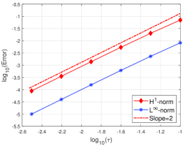
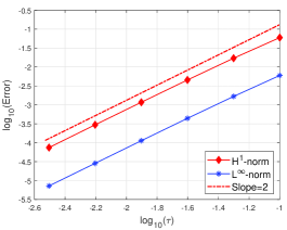
Figure 1. The error behavior with respect to the time step size for the CN scheme (2.11) with uniform time steps. Left: $M(\phi)\equiv 1$; right: $M(\phi)=1-\phi^{2}$.

Table 1. Numerical solution errors and convergence rates of the CN scheme (2.11) with nonuniform time steps.

Time steps			$M(\phi)=1$				$M(\phi)=1-\phi^{2}$
$N$	$\tau$	$\max\{\gamma_{n}\}$	$e^{T}_{H^{1}_{h}}$	Order	$e^{T}_{\infty}$	Order	$e^{T}_{H^{1}_{h}}$	Order	$e^{T}_{\infty}$	Order
$10$	1.629e-1	4.322	9.236e-2	–	1.090e-2	–	7.823e-2	–	7.927e-3	–
$20$	8.254e-2	4.660	2.768e-2	1.77	3.198e-3	1.80	2.334e-2	1.78	2.310e-3	1.81
$40$	3.953e-2	4.950	6.721e-3	1.92	7.659e-4	1.94	5.657e-3	1.93	5.511e-4	1.95
$80$	2.105e-2	6.901	1.933e-3	1.98	2.184e-4	1.99	1.625e-3	1.98	1.569e-4	1.99
$160$	1.075e-2	6.997	4.562e-4	2.15	5.141e-5	2.15	3.838e-4	2.15	3.689e-5	2.15
$320$	5.546e-3	8.084	1.119e-4	2.12	1.261e-5	2.12	9.517e-5	2.11	8.980e-6	2.14

4.2. MBP preservation

To test the MBP preservation of the proposed CN scheme (2.11), we consider two well-known benchmark problems governed by the Allen-Cahn equations. One is the grain coarsening dynamic process and the other is the shrinking bubble problem [4].

The grain coarsening dynamics

In this numerical experiment, we investigate the coarsening dynamics governed by the Allen-Cahn equation (1.1) with a nonlinear degenerate mobility $M(\phi)=1-\phi^{2}$ and a random initial data ranging from $-0.1$ to $0.1$. The domain is set to be $\Omega=(0,1)^{2}$ with the width parameter $\varepsilon=1/256\approx 3.91e$-$3$, and the uniform spatial mesh with $h=1/256$ is used for spatial discretization. In particular, for such a nonlinear mobility function, it is of essential importance to preserve the numerical solution $\phi\in[-1,1]$ in the numerical algorithm. Otherwise, it may lead to the ill-posedness of the proposed numerical scheme, and the numerical solution blowing up during the time simulation, as shown in Fig. 2 (a).

The MBP preservation of the proposed CN scheme (2.11) is investigated for this example through a long time simulation up to $T=3000$ using the CN scheme (2.11) with several large time step sizes. We set $S_{1}=4/5$ satisfying the condition (2.9), and choose two values for the stabilizing parameter $S_{2}$: one is the case of $S_{0}=0$ leading to the conditional MBP preservation of the CN scheme, the other is $S_{2}=\big{(}\frac{S_{1}}{4}+\frac{L\varepsilon^{2}}{h^{2}}\big{)}^{2}$ satisfying (2.15) to guarantee the unconditional MBP preservation of the CN scheme (2.11) as stated in Theorem 2.1. The evolutions of the supremum norm and energy of the simulated solutions for both cases are presented in Fig. 2. We observe that the CN scheme (2.11) with $S_{2}=0$ and $\tau=2$ preserve the MBP, and the numerical solutions blow up at a finite time about $t=30$, see 2-(a). It is also seen in Fig. 2-(b) that the CN scheme preserve the MBP under all tested time step sizes when the two stabilizing parameters $S_{1}$ and $S_{2}$ satisfy the conditions (2.9) and (2.15), respectively; furthermore, it also achieves energy dissipation for all cases in the sense of $E_{h}(\phi^{n+1})\leq E_{h}(\phi^{n})$ for $n=0,\cdots,N-1$.

One of main advantages of the unconditionally stable schemes is that it can be easily adopted by an adaptive time strategy. This is particularly useful for the long time simulation of the coarsening dynamic process, in which the phase transition usually goes through several different stages within a long period: changes quickly at the beginning and then rather slowly until it reaches a steady state. There already exist several efficient time-adaptive strategies [13, 14, 28, 34, 31, 32] that can be used in conjunction with numerical schemes with variable time steps. We will exploit the use of the following robust time adaptive strategy with the CN scheme (2.11) in the simulation, which is based on the energy variation [31] to efficiently simulate the coarsening dynamic process:

$$\tau_{n+1}=\max\big{(}\tau_{min},\frac{\tau_{max}}{\sqrt{1+\alpha|E^{{}^{\prime}}(t)|^{2}}}\big{)},$$ (4.1)

where $\tau_{min},\tau_{max}$ are the predetermined minimum and maximum time step sizes, and $\alpha$ is a positive constant parameter. Obviously according to this type of time strategy, the numerical scheme will automatically select large time step sizes when energy variation is big and a small ones otherwise. The parameters are set to be $\tau_{min}=10^{-5}$, $\tau_{max}=0.1$, and $\alpha=10^{5}$ in this test. In the simulation, we choose $S_{1}=4/5$ and $S_{2}=\big{(}\frac{S_{1}}{4}+\frac{L\varepsilon^{2}}{h^{2}}\big{)}^{2}$ such that both of the conditions (2.9) and (2.15) are satisfied. As shown in Fig. 4-(a), the CN scheme always preserves the MBP property during the simulation up to $T=150000.$ Moreover, we also display several snapshots of the simulated phase structures (around the times $t=500,1000,5000,10000,13000,15000$) in Fig. 3, and the evolutions of the energy and the adaptive time step sizes in Fig. 4-(b)&(c). As shown in Fig. 4-(b)&(c), the computed energy is always dissipative in time and the adaptive time stepping strategy scheme automatically select the time step sizes according the changing rate of the free energy, which demonstrates the efficiency of our proposed scheme adopted with the time adaptive strategy (4.1).

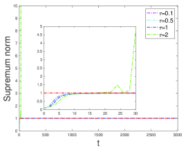
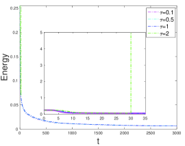
(a) $S_{1}=\frac{4}{5}$ and $S_{2}=0$

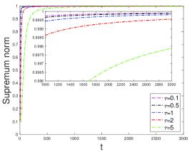
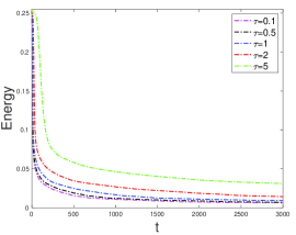
(b) $S_{1}=\frac{4}{5}$ and $S_{2}=\big{(}\frac{S_{1}}{4}+\frac{L\varepsilon^{2}}{h^{2}}\big{)}^{2}$

Figure 2. The evolutions in time of the supremum norm (left) and the energy (right) of the simulated solution produced by the CN scheme (2.11) with some uniform time steps for the grain coarsening problem with the degenerate mobility.

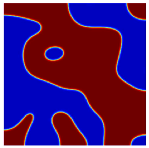
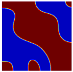
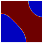
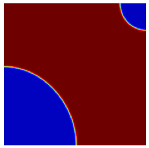
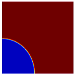
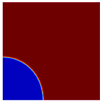
Figure 3. Snapshots of the simulated phase structures around the times $t=500$, $1000$, $5000$, $10000$, $13000$, and $15000$ produced by the CN scheme (2.11) with the time adaptive strategy (4.1) for the grain coarsening problem with the degenerate mobility.

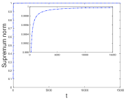
(a) the supremum norm

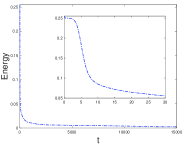
(b) the energy

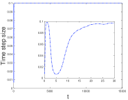
(c) the time step size

Figure 4. The evolutions in time of the supremum norm, the energy, and the time step sizes produced by the CN scheme (2.11) with the time adaptive strategy (4.1) for the grain coarsening problem (4.1) with the degenerate mobility.

The shrinking bubble problem

We next use the shrinking bubble problem [4] to test the performance of the proposed CN scheme (2.11) again with the time adaptive strategy (4.1). The shrinking bubble problem is driven by the Allen-Cahn equation (1.1) with $M(\phi)\equiv 1$ and $\varepsilon=0.01$ in a rectangular domain $(-0.5,0.5)^{2}$. The initial bubble is a sphere of radius $R_{0}=0.2$ located at the center of the computational domain, given by

$$\phi_{0}({\tenbi x})=\begin{cases}\begin{array}[]{r@{}l}1,&\quad|{\tenbi x}|^{2}<0.2^{2},\\[1.0pt] -1,&\quad|{\tenbi x}|^{2}\geq 0.2^{2}.\end{array}\end{cases}$$

As stated in [23, 11, 6], such a bubble is not stable and will shrink and finally disappear due the interface driving force. Moreover, with assumption of a sufficient small $\varepsilon$, the radius of the circle at time t can be approximately expressed as follows

$$R(t)=\sqrt{R^{2}_{0}-2\varepsilon^{2}t}.$$ (4.2)

We perform the simulation by combining the CN scheme (2.11) with $h=1/512$ and the time adaptive strategy (4.1) with $\tau_{min}=10^{-5}$, $\tau_{max}=0.01$, and $\alpha=10^{5}$. Several snapshots of the computed bubble at the times $t=0,20,80,120,180,200$ are plotted in Fig. 5, showing that the bubble disappears at $t=200$ as predicted. Moreover, it is observed in Fig. 6 (a) that the simulated radius of the bubble is monotonously decreasing with a rate almost identical to the theoretical prediction (4.2). Furthermore, we present the evolution of the supremum norm of the numerical solutions along with the time in Fig. 6-(b), which shows the MBP preservation of the proposed CN scheme (2.11) during the whole simulation. In the last line of Fig. 6, we plot the evolutions of the energy and the adaptive time step sizes to numerically demonstrate the energy dissipation and the efficiency of the proposed CN scheme (2.11) adopted with the time adaptive strategy (4.1).

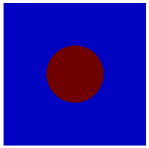
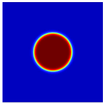
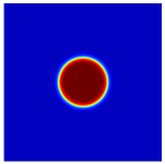
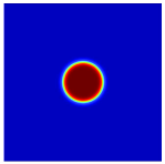
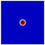
Figure 5. Snapshots of the simulated phase structures at the times $t=0$, $20$, $80$, $120$, $180$, and $200$ produced by the CN scheme (2.11) for with the time adaptive strategy (4.1) for the shrinking bubble problem.

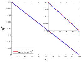
(a) the radius

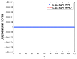
(b) the supremum norm

(c) the energy

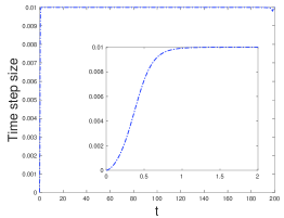
(d) the time step size

Figure 6. The evolutions in time of the radius, the supremum norm, and the energy of the simulated solution and the time step size produced by the CN scheme (2.11) with the adaptive time stepping approach (4.1) for the shrinking bubble problem.

5. Concluding remarks

A linear doubly stabilized CN scheme is constructed for the Allen-Cahn equation with general mobility in this paper. The resulting fully-discrete system is formed by applying the central finite difference method for spatial discretization, and requires two Poisson-type equations to be solved at each time step. Two stabilizing terms are introduced to unconditionally preserve the discrete MBP of the proposed scheme. The discrete $H^{1}$ and $L^{\infty}$ error estimates are rigorously derived for the constant mobility case and the general one, respectively. Furthermore, the corresponding energy stability of the proposed scheme is also established for both cases. Finally, a series of numerical experiments were carried out to verify the theoretical claims and illustrate the efficiency of the doubly stabilized CN scheme with a time adaptive strategy. It remains interest to further theoretically explore the unconditional energy dissipation preservation of the proposed scheme, which has been numerically observed in our numerical experiment.

References

- [1] A. Baskaran, Z. Hu, J. S. Lowengrub, C. Wang, S. M. Wise, and P. Zhou. Energy stable and efficient finite-difference nonlinear multigrid schemes for the modified phase field crystal equation. J. Comput. Phys., 250:270–292, 2013.
- [2] A. Baskaran, J. S. Lowengrub, C. Wang, and S. M. Wise. Convergence analysis of a second order convex splitting scheme for the modified phase field crystal equation. SIAM J. Numer. Anal., 51(5):2851–2873, 2013.
- [3] Y. Cai, L. Ju, R. Lan, and J. Li. Stabilized exponential time differencing schemes for the convective Allen–Cahn equation. Commun. Math. Sci., 21(1):127–150, 2023.
- [4] L. Chen and J. Shen. Applications of semi-implicit fourier-spectral method to phase field equations. Comput. Phys. Commun., 108(2-3):147–158, 1998.
- [5] X. Chen, X Qian, and S. Song. Fourth–order structure–preserving method for the conservative Allen–Cahn equation. Adv. Appl. Math. Mech., 15(1):159–181, 2023.
- [6] J. M. Church, Z. Guo, P. K. Jimack, A. Madzvamuse, K. Promislow, B. Wetton, S. M. Wise, and F. Yang. High accuracy benchmark problems for Allen-Cahn and Cahn-Hilliard dynamics. Commun. Comput. Phys., 26(4):947–972, 2019.
- [7] Q. Du, L. Ju, X. Li, and Z. Qiao. Maximum principle preserving exponential time differencing schemes for the nonlocal Allen–Cahn equation. SIAM J. Numer. Anal., 57(2):875–898, 2019.
- [8] Q. Du, L. Ju, X. Li, and Z. Qiao. Maximum bound principles for a class of semilinear parabolic equations and exponential time differencing schemes. SIAM Rev., 63(2):317–359, 2021.
- [9] X. Feng, H. Song, T. Tang, and J. Yang. Nonlinear stability of the implicit–explicit methods for the Allen–Cahn equation. Inverse Probl. Imag., 7(3), 2013.
- [10] Z. Fu and J. Yang. Energy-decreasing exponential time differencing Runge–Kutta methods for phase-field models. J. Comput. Phys., 454:110943, 2022.
- [11] D. Hou, M. Azaiez, and C. Xu. A variant of scalar auxiliary variable approaches for gradient flows. J. Comput. Phys., 395:307–332, 2019.
- [12] D. Hou, L. Ju, and Z. Qiao. A linear second–order maximum bound principle–preserving BDF scheme for the Allen–Cahn equation with a general mobility. Math. Comput., pages 1–28, 2023. https://doi.org/10.1090/mcom/3843.
- [13] D. Hou and Z. Qiao. An implicit–explicit second–order BDF numerical scheme with variable steps for gradient flows. J. Sci. Comput., 94(2):39, 2023.
- [14] D. Hou and Z. Qiao. A linear adaptive second–order backwarddifferentiation formulation scheme for phase field crystal equation. Numer. Methods Partial Differ. Eq., pages 1–22, 2023. https://doi.org/10.1002/num.23041.
- [15] T. Hou and H. Leng. Numerical analysis of a stabilized Crank–Nicolson/Adams–Bashforth finite difference scheme for Allen–Cahn equations. Appl. Math. Lett., 102:106150, 2020.
- [16] T. Hou, T. Tang, and J. Yang. Numerical analysis of fully discretized Crank–Nicolson scheme for fractional-in-space Allen–Cahn equations. J. Sci. Comput., 72(3):1214–1231, 2017.
- [17] Z. Hu, S. M. Wise, C. Wang, and J. S. Lowengrub. Stable and efficient finite-difference nonlinear-multigrid schemes for the phase field crystal equation. J. Comput. Phys., 228(15):5323–5339, 2009.
- [18] Q. Huang, K. Jiang, and J. Li. Exponential time differencing schemes for the Peng-Robinson equation of state with preservation of maximum bound principle. Adv. Appl. Math. Mech, 14(2):494–527, 2022.
- [19] K. Jiang, L. Ju, J. Li, and X. Li. Unconditionally stable exponential time differencing schemes for the mass-conserving allen–cahn equation with nonlocal and local effects. Numer. Methods Partial Differ. Equ., 38(6):1636–1657, 2022.
- [20] L. Ju, X. Li, and Z. Qiao. Generalized SAV–exponential integrator schemes for Allen–Cahn type gradient flows. SIAM J. Numer. Anal., 60(4):1905–1931, 2022.
- [21] L. Ju, X. Li, and Z. Qiao. Stabilized exponential–SAV schemes preserving energy dissipation law and maximum bound principle for the Allen–Cahn type equations. J. Sci. Comput., 92(2):66, 2022.
- [22] L. Ju, X. Li, Z. Qiao, and J. Yang. Maximum bound principle preserving integrating factor Runge–Kutta methods for semilinear parabolic equations. J. Comput. Phys., 439:110405, 2021.
- [23] L. Ju, J. Zhang, L. Zhu, and Q. Du. Fast explicit integration factor methods for semilinear parabolic equations. J. Sci. Comput., 62(2):431–455, 2015.
- [24] B. Li, J. Yang, and Z. Zhou. Arbitrarily high-order exponential cut-off methods for preserving maximum principle of parabolic equations. SIAM J. Sci. Comput., 42(6):A3957–A3978, 2020.
- [25] J. Li, L. Ju, Y. Cai, and X. Feng. Unconditionally maximum bound principle preserving linear schemes for the conservative Allen–Cahn equation with nonlocal constraint. J. Sci. Comput., 87(3):98, 2021.
- [26] J. Li, X. Li, L. Ju, and X. Feng. Stabilized integrating factor Runge–Kutta method and unconditional preservation of maximum bound principle. SIAM J. Sci. Comput., 43(3):A1780–A1802, 2021.
- [27] X. Li, J. Shen, and H. Rui. Energy stability and convergence of SAV block-centered finite difference method for gradient flows. Math. Comput., 88(319):2047–2068, 2019.
- [28] H. Liao, T. Tang, and T. Zhou. On energy stable, maximum-principle preserving, second order BDF scheme with variable steps for the Allen-Cahn equation. SIAM J. Numer. Anal., 58(4):2294–2314, 2020.
- [29] C. Liu, Z. Qiao, and Q. Zhang. Two-phase segmentation for intensity inhomogeneous images by the Allen-Cahn local binary fitting model. SIAM J. Sci. Comput., 44(1):B177 – B196, 2022.
- [30] C. Nan and H. Song. The high-order maximum-principle-preserving integrating factor Runge-Kutta methods for nonlocal Allen-Cahn equation. J. Comput. Phys., 456:111028, 2022.
- [31] Z. Qiao, Z. Zhang, and T. Tang. An adaptive time-stepping strategy for the molecular beam epitaxy models. SIAM J. Sci. Comput., 33(3):1395–1414, 2011.
- [32] J. Shen, T. Tang, and J. Yang. On the maximum principle preserving schemes for the generalized Allen–Cahn equation. Commun. Math. Sci., 14(6):1517–1534, 2016.
- [33] J. Shen, C. Wang, X. Wang, and S. M. Wise. Second-order convex splitting schemes for gradient flows with ehrlich–schwoebel type energy: application to thin film epitaxy. SIAM J. Numer. Anal., 50(1):105–125, 2012.
- [34] J. Shen, J. Xu, and J. Yang. A new class of efficient and robust energy stable schemes for gradient flows. SIAM Rev., 61(3):474–506, 2019.
- [35] T. Tang and J. Yang. Implicit–explicit scheme for the Allen–Cahn equation preserves the maximum principle. J. Comput. Math., 34(5):451–461, 2016.
- [36] A. Weiser and M. F. Wheeler. On convergence of block-centered finite differences for elliptic problems. SIAM J. Numer. Anal., 25(2):351–375, 1988.
- [37] S. M. Wise. Unconditionally stable finite difference, nonlinear multigrid simulation of the Cahn-Hilliard-Hele-Shaw system of equations. J. Sci. Comput., 44(1):38–68, 2010.
- [38] S. M. Wise, C. Wang, and J. S. Lowengrub. An energy-stable and convergence finite–difference scheme for the phase field crystal equation. SIAM J. Numer. Anal., 47(1):2269–2288, 2009.
- [39] X. Xiao, R. He, and X. Feng. Unconditionally maximum principle preserving finite element schemes for the surface Allen–Cahn type equations. Numer. Methods Partial Differ. Equ., 36(2):418–438, 2020.
- [40] J. Yang, Z. Yuan, and Z. Zhou. Arbitrarily high-order maximum bound preserving schemes with cut-off postprocessing for Allen–Cahn equations. J. Sci. Comput., 90:76, 2022.
- [41] H. Zhang, J. Yan, X. Qian, X. Chen, and S. Song. Explicit third-order unconditionally structure-preserving schemes for conservative Allen–Cahn equations. J. Sci. Comput., 90:8, 2022.
- [42] H. Zhang, J. Yan, X. Qian, X. M. Gu, and S. Song. On the maximum principle preserving and energy stability of high-order implicit-explicit Runge-Kutta schemes for the space-fractional Allen-Cahn equation. Numer. Algor., 88:1309–1336, 2021.
- [43] H. Zhang, J. Yan, X. Qian, and S. Song. Numerical analysis and applications of explicit high order maximum principle preserving integrating factor Runge-Kutta schemes for Allen–Cahn equation. Appl. Numer. Math., 161:372–390, 2021.