Classification of the anyon sectors of Kitaev’s quantum double model

Abstract

We give a complete classification of the anyon sectors of Kitaev’s quantum double model on the infinite triangular lattice and for finite gauge group $G$, including the non-abelian case. As conjectured, the anyon sectors of the model correspond precisely to the irreducible representations of the quantum double algebra of $G$.

Our proof consists of two main parts. In the first part, we construct for each irreducible representation of the quantum double algebra a pure state and show that the GNS representations of these pure states are pairwise disjoint anyon sectors. In the second part we show that any anyon sector is unitarily equivalent to one of the anyon sectors constructed in the first part.

Purity of the states constructed in the first part is shown by characterising these states as the unique states that satisfy appropriate local constraints. These constraints are of two types, namely flux constraints and gauge constraints. The flux constraints single out certain string-net states, while the gauge constraints fix the way in which these string-nets condense. At the core of the proof is the fact that certain groups of local gauge transformations act freely and transitively on collections of local string-nets. The proof that the GNS representations of these states are anyon sectors relies on showing that they are unitarily equivalent to amplimorphism representations which are much easier to compare to the ground state representation.

For the second part, we show that any anyon sector contains a pure state that satisfies all but a finite number of the constraints characterising the pure states of the first part. Using known techniques we can then construct a pure state in the anyon sector that satisfies all but one of these constraints. Finally, we show that any such state must be a vector state in one of the anyon sectors constructed in the first part.

1 Introduction

Over the decades since the discovery of the integer quantum Hall effect, the notion of topological phases of matter has come to be a central paradigm in condensed matter physics. In contrast to the conventional Landau-Ginsburg paradigm of spontaneous symmetry breaking, topological phases of matter are not distinguished by any local order parameter. Instead they are characterised by a remarkably wide variety of topological properties, ranging from toplogically non-trivial Bloch bands to topological ground-state degeneracy. What all these topological materials seem to have in common is that they are characterised by robust patterns in the entanglement structure of their ground states [LH08, Fid10].

Within this zoo of topological phases, the topologically ordered phases in two dimensions have received a great deal of attention. The reason for this is in part because of their possible applications to quantum computation [Kit03, Fre98, Nay+08]. Topologically ordered materials exhibit robust ground state degeneracy depending on the genus of the surface on which they sit, and they support anyon excitations which have mutual braiding statistics that differs from that of bosons or fermions.

With applications to quantum computation in mind, it is desirable to understand topological order from a microscopic point of view. On the one hand, an important role is played in this endeavor by exactly solvable quantum spin models that exhibit topologcial order, such as Kitaev’s quantum double models [Kit03] and, more generally, the Levin-Wen models [LW04]. On the other hand, one wants to obtain a good understanding of the mathematical structures involved in characterising topological orders in general models [Kit06, SKK20, KL20]. The latter problem has proven to be a rich challenge for mathematical physics [Naa11, Naa12, CNN18, CNN20, Oga22]. These works have yielded a rigorous, albeit still incomplete, description of topological order in gapped quantum spin systems in two dimensions. They provide robust definitions of anyon types, their fusion rules, and their braiding statistics, as well as a rigorous understanding of how these data fit together in a braided $C^{*}$-tensor category.

In this paper we study Kitaev’s quantum double models from this mathematical physics point of view. The quantum double models can be thought of as discrete gauge theories with a finite gauge group $G$. These models are of particular interest because for non-abelian $G$, they are paradigmatic examples of models that support non-abelian anyons, which could be used to build a universal quantum computer [Kit03]. We take a first step towards integrating the quantum double models for general $G$ into the mathematical framework referred to above. In particular, we classify all the anyon types of these models.

Roughly, an anyon type corresponds to a superselection sector that is unitarily equivalent to the ground state sector when restricted to any cone-like region of the plane. We call such sectors anyon sectors. Intuitively an anyon sector contains states that can be made to look like the ground state locally by moving the anyon somewhere else, but globally, the anyon is always detectable by braiding operations.

In order to completely classify the anyon sectors of the quantum double model we proceed as follows. First we prove that the frustration free ground state $\omega_{0}$ of the model is unique and therefore pure. It is important to understand the ground state well, because the notion of anyon sector is defined with respect to it. Uniqueness of the frustration free ground state is established by proving that the local constraints of the quantum double model determine expectation values of local observables completely. This is achieved by providing a description of the frustration free ground state as a string-net condensate and noting that local gauge groups of the model act freely and transitively on such string-nets. This result amounts to establishing local topological quantum order [BH11, BHM10] for Kitaev’s quantum double model, which is important for the interpretation of the model as a quantum error correcting code. The same result was obtained in [Naa12a], see also [Cui+20] for a similar result obtained by similar methods.

Next, we construct states $\omega_{s}^{RC;u}$ labeled by an irreducible representation $RC$ of the quantum double algebra $\mathcal{D}(G)$, a site $s$, and additional microscopic data $u$. These states look like the ground state when evaluated on any local observable whose support does not contain or encircle the site $s$. We characterise these states by showing that they are the unique states that satisfy certain local constraints depending on the site $s$ and the data $RC$ and $u$. In particular, the states $\omega_{s}^{RC;u}$ are pure. The techniques are similar to the ones used to prove uniqueness of the frustration free ground state but technically more involved. We continue by showing that the pure states $\omega_{s}^{RC;u}$ belong to different superselection sectors if and only if they differ in their $RC$ label. It follows that the GNS representations of the states $\omega_{s}^{RC;u}$ give us a collection of pairwise disjoint irreducible sectors $\pi^{RC}$ labeled by irreducible representations of the quantum double algebra. By relating the sectors $\pi^{RC}$ to so-called amplimorphism representations [Naa15, Vec94, FGV94, NS97], we show that these sectors are in fact anyon sectors. Finally, we show that any anyon sector must contain one of the states $\omega_{s}^{RC;u}$, thus showing that all anyon sectors are equivalent to one of the $\pi^{RC}$.

The paper is structured as follows. In Section 2 we set up the problem and state our main results. In Section 3 we show existence and uniqueness of the frustration free ground state of the quantum double model. In Section 4 we construct the states $\omega_{s}^{RC;u}$ that ‘contain an anyon’ at site $s$ and prove that these states are pure. Section 5 is devoted to constructing for each irreducible representation $RC$ of the quantum double algebra a superselection sector $\pi^{RC}$ that contains the states $\{\omega_{s}^{RC;u}\}_{s,u}$, and proving that they are disjoint anyon sectors. Finally, in section 6 we show that any anyon sector is unitarily equivalent to one of the $\pi^{RC}$, thus showing that the $\pi^{RC}$ exhaust all anyon sectors of the model.

2 Setup and main results

2.1 Algebra of observables

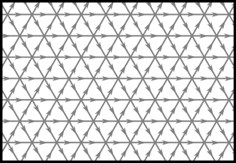
Figure 1: A snapshot of the triangular lattice with all edges oriented towards the right.

Let $\Gamma$ be the regular triangular lattice whose set of vertices $\Gamma^{V}$ we regard as a subset of the plane $\mathbb{R}^{2}$ such that nearest neighbouring vertices are separated by unit distance. Denote the set of edges and the set of faces of $\Gamma$ by $\Gamma^{E}$ and $\Gamma^{F}$ respectively. We think of each $e\in\Gamma^{E}$ as having a fixed orientation, which is arbitrarily chosen to be pointing to the right for all edges, see Figure 1. We identify each edge $e\in\Gamma^{E}$ with the pair $(v_{0},v_{1})$ of neighbouring vertices such that $v_{0}$ is the initial, and $v_{1}$ the final vertex of $e$ with this orientation, so $\Gamma^{E}$ is a subset of the set of oriented edges of $\Gamma$ given by

$$\overrightarrow{\Gamma}^{E}:=\{(v_{0},v_{1})\in\Gamma^{V}\times\Gamma^{V}\,:\,v_{0}\,\text{and}\,v_{1}\,\text{are nearest neighbours}\}.$$

Any oriented edge $e=(v_{0},v_{1})$ has an initial vertex $\partial_{0}e=v_{0}$, a final vertex $\partial_{1}e=v_{1}$ and an opposite edge $\bar{e}=(v_{1},v_{0})$. The vertices are equipped with the graph distance $\mathrm{dist}(\cdot,\cdot)$ and similarly for the faces (regarded as elements of the dual graph).

We fix a finite group $G$ and associate to each edge $e\in\Gamma^{E}$ a Hilbert space $\mathcal{H}_{e}=\mathbb{C}^{|G|}$ and the algebra $\mathfrak{A}_{e}=\mathrm{End}(\mathcal{H}_{e})$ of matrices over $\mathcal{H}_{e}$. For any finite $S\subset\Gamma^{E}$ we have a Hilbert space $\mathcal{H}_{S}=\otimes_{e\in S}\mathcal{H}_{e}$ and the algebra of operators $\mathfrak{A}_{S}=\mathrm{End}(\mathcal{H}_{S})$ on this space.

Let $S_{1},S_{2}\subset\Gamma^{E}$ be finite sets of edges such that $S_{1}\subset S_{2}$ then there is a natural embedding $\iota_{S_{1},S_{2}}:\mathfrak{A}_{S_{1}}\hookrightarrow\mathfrak{A}_{S_{2}}$ given by tensoring with the identity, i.e.

$$\iota_{S_{1},S_{2}}(O)=O\otimes\mathds{1}_{\mathfrak{A}_{S_{2}\setminus S_{1}}}$$

for all $O\in\mathfrak{A}_{S_{1}}$. With these embeddings, the algebras $\mathfrak{A}_{S}$ for finite $S\subset\Gamma^{E}$ form a directed system of matrix algebras. Their direct limit is called the local algebra, and is denoted by $\mathfrak{A}_{loc}$. The norm closure of the local algebra

$$\mathfrak{A}=\overline{\mathfrak{A}_{loc}}^{||\cdot||}$$

is called the quasi-local algebra or observable algebra.

Similarly, for any (possibly infinite) $S\subset\Gamma^{E}$ we have the algebra $\mathfrak{A}_{S}\subset\mathfrak{A}$ of quasi-local observables supported on $S$.

A state on $\mathfrak{A}$ is a positive linear functional $\omega:\mathfrak{A}\rightarrow\mathbb{C}$ with $\omega(\mathds{1})=1$. Given a state $\omega$ on $\mathfrak{A}$ there is a representation $\pi_{\omega}:\mathfrak{A}\rightarrow\mathcal{B}({\mathcal{H}_{\omega}})$ for some separable Hilbert space $\mathcal{H}_{\omega}$ containing a unit vector $\ket{\Omega}$ that is cyclic for the representation $\pi_{\omega}$ and such that $\omega(O)=\langle\Omega,\pi_{\omega}(O)\Omega\rangle$ for all $O\in\mathfrak{A}$. The triple $(\pi_{\omega},\mathcal{H}_{\omega},\ket{\Omega})$ satisfying these properties is unique up to unitary equivalence, and is called the GNS triple of the state $\omega$.

Throughout this paper, we will use the word ‘projector’ to mean a self-adjoint operator that squares to itself. A collection of projectors is called orthogonal if the product of each pair of projectors in the set vanishes. A set of projectors is called commuting if each pair of projectors in the set commutes with each other.

2.2 The quantum double Hamiltonian and its frustration free ground state

We say an edge $e$ belongs to a face $f$ and write $e\in f$ when $e$ is an edge on the boundary of $f$. Similarly, we say a vertex $v$ belongs to $f$ and write $v\in f$ if $v$ neighbours $f$, and we say a vertex $v$ belongs to an edge $e$ and write $v\in e$ if $v$ is the origin or endpoint of $e$.

We fix for each edge $e$ an orthonormal basis $\{\ket{g}\}_{g\in G}$ for $\mathcal{H}_{e}$ labelled by elements of the group $G$. For $g\in G$ we denote its inverse by $\overline{g}$, and we define the left group action $L_{e}^{h}:=\sum_{g\in G}\ket{hg}\bra{g}$, the right group action $R^{h}_{e}:=\sum_{g\in G}\ket{g\bar{h}}\bra{g}$, and the projectors $T_{e}^{g}:=\ket{g}\bra{g}$.

For each vertex $v$ and edge $e$ such that $v$ belongs to $e$ we set $L^{h}(e,v)=L^{h}_{e}$ if $\partial_{0}e=v$ and $L^{h}(e,v)=R^{h}_{e}$ if $\partial_{1}e=v$. We then define the gauge constraint

$$A_{v}:=\frac{1}{\absolutevalue{G}}\sum_{h\in G}\,\prod_{e\in v}L^{h}(e,v),$$

which is a projector. Similarly, for each face $f$ and edge $e\in f$ we set $T^{h}(e,f)=T_{e}^{h}$ if $e$ is oriented counterclockwise around $f$, and $T^{h}(e,f)=T_{e}^{\bar{h}}$ if $e$ is oriented clockwise around $f$. If the face $f$ has bounding edges $(e_{1},e_{2},e_{2})$ ordered counterclockwise (with arbitrary initial edge), then we define the flat gauge projector

$$B_{f}:=\sum_{\begin{subarray}{c}g_{1},g_{2},g_{3}\in G:\\ g_{1}g_{2}g_{3}=1\end{subarray}}T^{g_{1}}(e_{1},f)\,T^{g_{2}}(e_{2},f)\,T^{g_{3}}(e_{3},f),$$

which is also a projector (Lemma A.1). Note that this expression does not depend on which edge goes first in the triple $(e_{1},e_{2},e_{3})$. Note further that $\{A_{v}\}_{v\in\Gamma^{V}}\cup\{B_{f}\}_{f\in\Gamma^{F}}$ is a set of commuting projectors (Lemma A.1).

The quantum double Hamiltonian is the formal sum (interaction) of commuting projectors

$$H=\sum_{v\in\Gamma^{V}}(\mathds{1}-A_{v})+\sum_{f\in\Gamma^{F}}(\mathds{1}-B_{f}).$$

A state $\omega$ minimises the energy for this Hamiltonian if it minimizes the expectation value of each term individually.

Definition 2.1.

A state $\omega$ on $\mathfrak{A}$ is a frustration free ground state of $H$ if $\omega(A_{v})=\omega(B_{f})=1$ for all $v\in\Gamma^{V}$ and all $f\in\Gamma^{F}$.

If a state $\omega$ satisfies $\omega(A_{v})=1$ then we say it is gauge-invariant at $v$, and if $\omega(B_{f})=1$ then we say it is flat at $f$. A frustration free ground state is gauge invariant and flat everywhere.

The following Theorem is proven in Section 3, Lemma 3.28.

Theorem 2.2.

The quantum double Hamiltonian has a unique frustration free ground state.

We will denote the unique frustration free ground state by $\omega_{0}$, and let $(\pi_{0},\mathcal{H}_{0},\ket{\Omega_{0}})$ be its GNS triple. Note that since $\omega_{0}$ is the unique frustration free ground state of the quantum double model, it is a pure state, and therefore $\pi_{0}$ is an irreducible representation.

2.3 Classification of anyon sectors

In the context of infinite volume quantum spin systems or field theories, types of anyonic excitations over a ground state $\omega_{0}$ have a very nice mathematical characterisation. They correspond to the irreducible representations of the observable algebra that satisfy a certain superselection criterion w.r.t. the GNS representation $\pi_{0}$ of the ground state ([DHR71], [DHR74], [FRS89], [FRS92], [FG90]). In our setting of quantum spin systems, the appropriate superselection criterion was first formulated in [Naa11] in the special case of the Toric code.

The cone with apex at $a\in\mathbb{R}^{2}$, axis $\hat{v}\in\mathbb{R}^{2}$ of unit length, and opening angle $\theta\in(0,2\pi)$ is the open subset of $\mathbb{R}^{2}$ given by

$$\Lambda_{a,\hat{v},\theta}:=\{x\in\mathbb{R}^{2}\,|\,(x-a)\cdot\hat{v}>\norm{x-a}\cos(\theta/2)\}.$$

Any subset $\Lambda\subset\mathbb{R}^{2}$ of this form will be called a cone. Denote by $\overline{\Lambda}\subset\Gamma^{E}$ the set of edges whose midpoints lie within the subset $\Lambda\subset\mathbb{R}^{2}$, and write $\mathfrak{A}_{\Lambda}:=\mathfrak{A}_{\overline{\Lambda}}$ for the algebra of observables supported on $\Lambda$. With this definition we have $\overline{\Lambda}\cup\overline{\Lambda^{c}}=\Gamma^{E}$ for any $\Lambda\subset\mathbb{R}^{2}$.

Definition 2.3.

An irreducible representation $\pi:\mathfrak{A}\rightarrow\mathcal{B}(\mathcal{H})$ is said to satisfy the superselection criterion w.r.t. $\pi_{0}$ if for any cone $\Lambda$, there is a unitary $U_{\Lambda}:\mathcal{H}_{0}\rightarrow\mathcal{H}$ such that

$$\pi(A)=U_{\Lambda}\pi_{0}(A)U^{*}_{\Lambda}$$

for all $A\in\mathfrak{A}_{\Lambda}$. We will call such a representation an anyon sector for $\omega_{0}$.

Let us denote by $\mathcal{D}(G)$ the quantum double algebra of $G$. The irreducible representations of $\mathcal{D}(G)$ are uniquely labeled by the following data (see for example [Gou93]):

• A conjugacy class $C$ of $G$.

• An irreducible representation $R$ of the group $N_{C}$ defined as follows. Pick a representative $r_{C}\in C$, and let $N_{C}=\{g\in G\,:\,r_{C}g=gr_{C}\}$ be the commutant of $r_{C}$ in $G$. The group structure of $N_{C}$, and therefore the set of its irreducible representations, is independent of the choice of $r_{C}\in C$.

We denote the irreducible representation of $\mathcal{D}(G)$ corresponding to conjugacy class $C$ and irreducible representation $R$ by $RC$.

Our main result is the complete classification of the anyon sectors of $\omega_{0}$ in terms of the irreducible representations of $\mathcal{D}(G)$.

Theorem 2.4.

For each irreducible representation $RC$ of $\mathcal{D}(G)$ there is an anyon sector $\pi^{RC}$. The representations $\{\pi^{RC}\}_{RC}$ are pairwise disjoint, and any anyon sector is unitarily equivalent to one of them.

This Theorem is restated and proven in Section 6, Theorem 6.14.

3 The frustration free ground state

In this section we prove Theorem 2.2, which says that the quantum double Hamiltonian has a unique frustration free ground state in infinite volume. The results obtained in this Section are actually a special case of those presented in the next Section 4, which handles states with a ‘single excitation’ above the ground state. We nevertheless present the analysis of the frustration free ground state separately because it allows us to introduce many concepts and definitions that will be essential in Section 4 in a simpler setting, making the presentations much clearer.

3.1 Ribbon operators, gauge configurations, and gauge transformations

Let $\Gamma^{*}$ be the dual lattice to $\Gamma$. To each edge $e\in\overrightarrow{\Gamma}^{E}$ we associate a unique oriented dual edge ${{e^{*}}}\in(\vec{\Gamma^{*}})^{E}$ with orientation such that along $e$, the dual edge ${{e^{*}}}$ passes from right to left. Here

$$(\vec{\Gamma^{*}})^{E}=\{(f_{0},f_{1})\in\Gamma^{F}\times\Gamma^{F}\,:\,f_{0}\,\text{and}\,f_{1}\,\text{are neighbouring faces}\}$$

is the set of oriented dual edges of $\Gamma$.

3.1.1 Sites and triangles

A site $s$ is a pair $s=(v,f)$ of a vertex and a face such that $v$ neighbours $f$. We write $v(s)=v$ for the vertex of $s$ and $f(s)=f$ for the face of $s$. We represent a site graphically by a line from the site’s vertex to the center of its face. A direct triangle $\tau=(s_{0},s_{1},e)$ consists of a pair of sites $s_{0},s_{1}$ that share the same face, and an edge $e\in\Gamma^{E}$ that connects the vertices of $s_{0}$ and $s_{1}$. We write $\partial_{0}\tau=s_{0}$ and $\partial_{1}\tau=s_{1}$ for the initial and final sites of the direct triangle $\tau$, and $e_{\tau}=(v(s_{0}),v(s_{1}))$ for the oriented edge associated to $\tau$. See Figure 2. The opposite triangle to $\tau$ is the direct triangle $\bar{\tau}=(s_{1},s_{0},e)$. Similarly, a dual triangle $\tau=(s_{0},s_{1},e)$ consists of a pair of sites $s_{0},s_{1}$ that share the same vertex, and the edge $e$ whose associated dual edge ${{e^{*}}}$ connects the faces of $s_{0}$ and $s_{1}$. We write again $\partial_{0}\tau=s_{0}$ and $\partial_{1}\tau=s_{1}$, $e^{*}_{\tau}=(f(s_{0}),f(s_{1}))$ for the oriented dual edge associated to $\tau$, and define an opposite dual triangle $\bar{\tau}=(s_{1},s_{0},e)$.

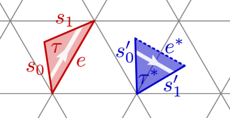
Figure 2: A direct triangle $\tau=(s_{0},s_{1},e)$ in red, and a dual triangle $\tau^{*}=(s^{\prime}_{0},s^{\prime}_{1},e^{\prime})$ in blue. The dual edge $e^{*}$ associated to $e^{\prime}$ is indicated as a dotted blue line.

To each dual triangle $\tau=(s_{0},s_{1},e)$ we associate unitaries $L^{h}_{\tau}$ supported on the edge $e$. The way $L^{h}_{\tau}$ acts depends on whether the dual edge $e^{*}$ dual to $e$ satisfies $e^{*}=(f(s_{0}),f(s_{1}))$ or $e^{*}=(f(s_{1}),f(s_{2}))$, and on whether $v(s_{0})=\partial_{0}e$ or $v(s_{0})=\partial_{1}e$ as follows. If $e^{*}=(f(s_{0}),f(s_{1}))$ and $v(s_{0})=\partial_{0}e$ then $L^{h}_{\tau}:=L_{e}^{h}$. If $e^{*}=(f(s_{0}),f(s_{1}))$ and $v(s_{0})=\partial_{1}e$ then $L^{h}_{\tau}:=R_{e}^{\bar{h}}$. If $e^{*}=(f(s_{1}),f(s_{0}))$ and $v(s_{0})=\partial_{0}e$ then $L^{h}_{\tau}:=L_{e}^{\bar{h}}$. Finally, If $e^{*}=(f(s_{1}),f(s_{0}))$ and $v(s_{0})=\partial_{1}e$ then $L^{h}_{\tau}:=R_{e}^{h}$. Similarly, to each direct triangle $\tau=(s_{0},s_{1},e)$ we associated projectors $T^{g}_{\tau}:=T^{g}_{e}$ if $e=(v(s_{0}),v(s_{1}))$ and $T^{g}_{\tau}:=T_{e}^{\bar{g}}$ if $e=(v(s_{1}),v(s_{0}))$.

3.1.2 Ribbons

We define a finite ribbon $\rho:=\{\tau_{i}\}_{i=1}^{l}$ to be an ordered tuple of triangles such that $\partial_{1}\tau_{i}=\partial_{0}\tau_{i+1}$ for all $i=1,\cdots,l-1$, and such that for each edge $e\in\Gamma^{E}$ there is at most one triangle $\tau_{i}$ for which $\tau_{i}=(\partial_{0}\tau_{i},\partial_{1}\tau_{i},e)$. We define $\partial_{0}\rho:=\partial_{0}\tau_{1}$ as the start of the ribbon and $\partial_{1}\rho:=\partial_{1}\tau_{n}$ as the end of the ribbon. See Figure 3. If all triangles belonging to a ribbon $\rho$ are direct, we say that $\rho$ is a direct ribbon, and if all triangles belonging to a ribbon $\rho$ are dual, we say that $\rho$ is a dual ribbon.

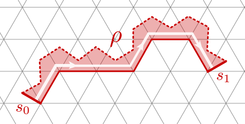
Figure 3: A finite ribbon $\rho$ with $\partial_{0}\rho=s_{0}$ and $\partial_{1}\rho=s_{1}$. The direct path of $\rho$ consists of the solid red edges.

If we have two tuples $\rho_{1}=\{\tau_{i}\}_{i=1}^{l_{1}}$ and $\rho_{2}=\{\tau_{i}\}_{i=l_{1}+1}^{l_{2}}$ then we can concatenate them to form a tuple $\rho=\{\tau_{i}\}_{i=1}^{l_{1}+l_{2}}$. We denote this concatenated tuple by $\rho=\rho_{1}\rho_{2}$. Note that if $\rho$ is a finite ribbon and $\rho=\rho_{1}\rho_{2}$, then $\rho_{1}$ and $\rho_{2}$ are automatically finite ribbons and (if $\rho_{1}$ and $\rho_{2}$ are non-empty), $\partial_{0}\rho=\partial_{0}\rho_{1}$, $\partial_{1}\rho=\partial_{1}\rho_{2}$ and $\partial_{1}\rho_{1}=\partial_{0}\rho_{2}$.

The empty ribbon is denoted by $\epsilon$. The orientation reversal of a ribbon $\rho=\{\tau_{i}\}_{i=1}^{l}$ is the ribbon $\bar{\rho}=\bar{\tau}_{l}\cdots\bar{\tau}_{1}$. We say a finite ribbon $\rho$ is closed if $\partial_{0}\rho=\partial_{1}\rho$.

The support of a ribbon $\rho=\{\tau_{i}\}_{i=1}^{l}$ is

$$\mathrm{supp}(\rho):=\{e\in\Gamma^{E}\,:\,e=e_{\tau_{i}}\,\,\text{or}\,\,\bar{e}=e_{\tau_{i}}\,\,\text{for some }\,i=1,\cdots,l\}.$$

If $\mathrm{supp}(\rho)\subseteq S\subseteq\Gamma^{E}$ we say $\rho$ is supported on $S$.

3.1.3 Direct paths

A direct path $\gamma=\{e_{i}\}_{i=1}^{l}$ is an ordered tuple of oriented edges $e_{i}\in\overrightarrow{\Gamma}^{E}$ such that $\partial_{1}e_{i}=\partial_{0}e_{i+1}$ for $i=1,\cdots,l-1$. We write $\partial_{0}\gamma=\partial_{0}e_{1}$ for the initial vertex, and $\partial_{1}\gamma=\partial_{1}e_{l}$ for the final vertex of $\gamma$. Given two direct paths $\gamma_{1}=\{e_{i}\}_{i=1}^{l_{1}}$ and $\gamma_{2}=\{e_{i}\}_{i=l_{1}+1}^{l_{1}+l_{2}}$ such that $\partial_{1}\gamma_{1}=\partial_{0}\gamma_{2}$ we can concatenate them to form a new direct path $\gamma=\{e_{i}\}_{i=1}^{l_{1}+l_{2}}$. We denote the concatenated path by $\gamma=\gamma_{1}\gamma_{2}$. The orientation reversal of a direct path $\gamma=\{e_{i}\}_{i=1}^{l}$ is the direct path $\bar{\gamma}=\bar{e}_{l}\cdots\bar{e}_{1}$. The support of a direct path $\gamma=\{e_{i}\}_{i=1}^{l}$ is

$$\mathrm{supp}(\gamma):=\{e\in\Gamma^{E}\,:\,e=e_{i}\,\,\text{or}\,\,\bar{e}=e_{i}\,\,\text{for some}\,\,i=1,\cdots,l\}.$$

If $\mathrm{supp}(\gamma)\subseteq S\subseteq\Gamma^{E}$ we say $\gamma$ is supported on $S$.

To each ribbon $\rho$ we can associate a direct path as follows. Let $\rho=\{\tau_{1},\cdots,\tau_{l}\}$ be a finite ribbon, and let $J=\{j_{1},\cdots,j_{l^{\prime}}\}\subset\{1,\cdots,l\}$ be the ordered subset such that $\tau_{j}$ is a direct triangle if and only if $j\in J$. Then $\rho^{dir}:=\{e_{\tau_{j}}\,:\,j\in J\}$ is the direct path of $\rho$. To see that this is indeed a direct path, take indices $j_{\nu},j_{\nu+1}\in J$ and suppose $j_{\nu+1}=j_{\nu}+m$. Then we want to show that $\partial_{1}e_{\tau_{j_{\nu}}}=\partial_{0}e_{\tau_{j_{\nu+1}}}$. By construction all triangles $\tau_{j_{\nu}+n}$ for $n=1,\cdots,m-1$ are dual and therefore $v=v(\partial_{0}\tau_{j_{\nu}+n})=v(\partial_{1}\tau_{j_{\nu}+n})$ are equal for all these $n$. We therefore have $\partial_{1}e_{\tau_{j_{\nu}}}=v(\partial_{1}\tau_{j_{\nu}})=v$ and $\partial_{0}e_{\tau_{j_{\nu}+m}}=v(\partial_{0}\tau_{j_{\nu+1}})=v$ as required. We have $\bar{\rho}^{dir}=\overline{\rho^{dir}}$, and if $\rho$ is supported in $S\subseteq\Gamma^{E}$ then $\rho^{dir}$ is also supported in $S$.

3.1.4 Ribbon operators

Here we introduce ribbon operators associated to any finite ribbon, and state some of their elementary properties. For proofs and many more properties, see Appendix A or appendices B and C of [BM08]. To each ribbon $\rho$ we associate a ribbon operator $F^{h,g}_{\rho}$ as follows. If $\epsilon$ is the trivial ribbon, then we set $F_{\epsilon}^{h,g}=\delta_{1,g}\mathds{1}$. For ribbons composed of a single direct triangle $\tau$ we put $F^{h,g}_{\tau}=T_{\tau}^{g}$. For ribbons composed of a single dual triangle $\tau$, we put $F^{h,g}_{\tau}=\delta_{g,1}L_{\tau}^{h}$. For longer ribbons the ribbon operators are defined inductively as

$$F^{h,g}_{\rho}=\sum_{k\in G}F^{h,k}_{\rho_{1}}F^{\overline{k}hk,\overline{k}g}_{\rho_{2}}$$

for $\rho=\rho_{1}\rho_{2}$. It follows from the discussion at the beginning of appendix A that this definition is independent of the way $\rho$ is split into two smaller ribbons. By construction, the ribbon operator $F_{\rho}^{h,g}$ is supported on $\mathrm{supp}(\rho)$. Let us define

$$T^{g}_{\rho}:=F^{1,g}_{\rho},\qquad L^{h}_{\rho}:=\sum_{g\in G}F^{h,g}_{\rho}$$

so that $F^{h,g}_{\rho}=L^{h}_{\rho}T^{g}_{\rho}=T^{g}_{\rho}L^{h}_{\rho}$ (Lemma A.2).

We can define gauge transformations $A_{s}^{h}$ and flux projectors $B_{s}^{g}$ at site $s$ in terms of the ribbon operators as follows:

$$A_{s}^{h}:=F^{h,1}_{\rho_{\star}(s)},\qquad B_{s}^{g}:=F^{1,\overline{g}}_{\rho_{\triangle}(s)}$$

where $\rho_{\triangle}(s)$ (resp. $\rho_{\star}(s)$) is the unique counterclockwise closed direct (dual) ribbon with end sites at $s$, see Figure 4. It is easily verified that $A_{s}^{h_{1}}A_{s}^{h_{2}}=A_{s}^{h_{1}h_{2}}$ for all $h_{1},h_{2}\in G$, so the gauge transformations at $s$ form a representation of $G$. Similarly, one verifies that $B_{s}^{g_{1}}B_{s}^{g_{2}}=\delta_{g_{1},g_{2}}B_{s}^{g_{1}}$ for all $g_{1},g_{2}\in G$. We further note that the gauge transformations $A_{s}^{h}$ depend only on the vertex $v(s)$, so we may put $A_{v}^{h}:=A_{s}^{h}$ for any site $s$ such that $v=v(s)$ and speak of the gauge transformations at the vertex $v$. Similarly, the projectors $B_{s}^{1}$ onto trivial flux depend only on the face $f(s)$ so we may put $B_{f}^{1}=B_{s}^{1}$ for any site $s$ such that $f=f(s)$.

The projectors $A_{v},B_{f}$ appearing in the quantum double Hamiltonian can now be written as follows:

$$A_{v}=\frac{1}{\absolutevalue{G}}\sum_{h}A_{v}^{h},\quad B_{f}=B_{f}^{1}.$$

They are the projectors onto states that are gauge invariant at $v$, and that have trivial flux at $f$, respectively.

Figure 4: The elementary direct ribbon $\rho_{\triangle}(s)$ associated to the site $s$, and the elementary dual ribbon $\rho_{\star}(s^{\prime})$ associated to the site $s^{\prime}$.

3.1.5 Gauge configurations and gauge transformations

It is very helpful to think of the frustration free ground state of the quantum double model as a string net condensate, see [LW04]. In what follows we establish the language of string-nets, which in this case correspond to gauge configurations. For any $S\subseteq\Gamma^{E}$ we denote by $\mathfrak{G}_{S}$ the set of maps $\alpha:S\rightarrow G$. We will denote by $\alpha_{e}$ the evaluation of $\alpha$ on an edge $e\in S$. We call such maps gauge configurations on $S$. Let us write $\overrightarrow{S}=\{e\in\overrightarrow{\Gamma}^{E}\,:\,e\in S\,\,\text{or}\,\,\bar{e}\in S\}$ for the set of oriented edges corresponding to $S$. Any gauge configuration $\alpha$ on $S\subseteq\Gamma^{E}$ extends to a function $\alpha:\overrightarrow{S}\rightarrow G$ on oriented edges by setting $\alpha_{\bar{e}}=\bar{\alpha}_{e}$. The meaning of $\alpha_{e}$ is the parallel transport of a discrete gauge field as one traverses the edge $e$.

For any finite $V\subset\Gamma^{V}$ we define $\mathcal{G}_{V}$ to be the group of unitaries generated by $\{A_{v}^{g_{v}}\,:\,v\in V,\,\,g_{v}\in G\}$. Any element $U\in\mathcal{G}_{V}$ is uniquely determined by an assignment $V\ni v\mapsto g_{v}\in G$ of a group element to each vertex in $V$ so that

$$U=U[\{g_{v}\}]=\prod_{v\in V}\,A_{v}^{g_{v}}.$$

We call $\mathcal{G}_{V}$ the group of gauge transformations on $V$.

If each $U\in\mathcal{G}_{V}$ is supported on a set $S\subseteq\Gamma^{E}$ then the gauge group $\mathcal{G}_{V}$ acts invertibly on the gauge configurations $\mathfrak{G}_{S}$ as follows. The gauge transformation $U=U[\{g_{v}\}]\in\mathcal{G}_{V}$ acts on a gauge configuration $\alpha\in\mathfrak{G}_{S}$, yielding a new gauge configuration $\alpha^{\prime}:=U(\alpha)\in\mathfrak{G}_{S}$ given by $\alpha^{\prime}_{e}=g_{\partial_{0}e}\,\alpha_{e}\,\bar{g}_{\partial_{1}e}$, where we set $g_{v}=1$ whenever $v\not\in R$.

If $S\subset\Gamma^{E}$ is finite then we let $\mathcal{H}_{S}:=\bigotimes_{e\in S}\mathcal{H}_{e}$. The set of gauge configurations $\mathfrak{G}_{S}$ then labels an orthonormal basis of $\mathcal{H}_{S}$ given by $\ket{\alpha}:=\bigotimes_{e\in S}\ket{\alpha_{e}}$. If the gauge transformations $\mathcal{G}_{V}$ for some finite $V\subset\Gamma^{V}$ are supported in $S$ then these gauge transformations act on the Hilbert space $\mathcal{H}_{S}$ as $U\ket{\alpha}=\ket{U(\alpha)}$, i.e. Gauge transformations map basis states to basis states.

We employ the following graphical representation of states $\ket{\alpha}$. For any edge $e$, the basis state $\ket{g}_{e}$ of $\mathcal{H}_{e}$ is represented by the edge $e$ being crossed from right to left by an oriented string labeled $g$. An equivalent representation of $\ket{g}_{e}$ is the edge $e$ being crossed from left to right by a string labeled $\bar{g}$, see Figure 5. The basis element $\ket{1}_{e}$ is represented by the edge $e$ not being crossed by any string at all.

A tensor product of several of such basis states is represented by a figure where each participating edge is crossed by a labeled oriented string by the rules just described. See Figure 6 for an example.

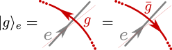
Figure 5: A graphical representation of the basis vector $\ket{g}_{e}\in\mathcal{H}_{e}$.

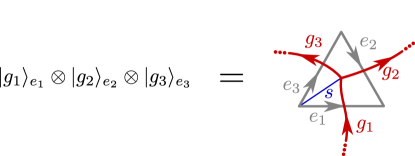
Figure 6: A graphical representation of the tensor product vector $\ket{g_{1}}_{e_{1}}\otimes\ket{g_{2}}_{e_{2}}\otimes\ket{g_{3}}_{e_{3}}\in\mathcal{H}_{\{e_{1},e_{2},e_{3}\}}$ for edges $e_{1},e_{2},e_{3}$ belonging to a single face $f$. We have also indicated a site $s$ with $f(s)=f$ in blue.

3.2 Local gauge configurations and boundary conditions

Recall that $\mathrm{dist}(\cdot,\cdot)$ is the graph distance on $\Gamma^{V}$. We fix an arbitrary site ${s_{0}}=(v_{0},f_{0})$ and define (see figure 7):

$${\Gamma}^{V}_{n}({s_{0}}) :=\{v\in\Gamma^{V}\,:\,\mathrm{dist}(v,v_{0})\leq n\},$$

$${\Gamma}^{F}_{n}({s_{0}}) :=\{f\in\Gamma^{F}\,:\,\exists v\in f\text{ such that }v\in{\Gamma}^{V}_{n}\},$$

$${\Gamma}^{E}_{n}({s_{0}}) :=\{e\in\Gamma^{E}\,:\,\exists f\in{\Gamma}^{F}_{n}\text{ such that }e\in f\},$$

$$\partial{\Gamma}^{E}_{n}({s_{0}}) :=\{e\in{\Gamma}^{E}_{n}\,:\,\exists!f\in{\Gamma}^{F}_{n}\text{ with }e\in f\},$$

$$\partial{\Gamma}^{V}_{n}({s_{0}}) :={\Gamma}^{V}_{n+1}\setminus{\Gamma}^{V}_{n}.$$

Note that these regions depend on the choice of an origin ${s_{0}}$. Throughout this paper, we will want to consider different sites as the origin. In order to unburden the notation we will nevertheless drop ${s_{0}}$ from the notation and simply write ${\Gamma}^{V}_{n},{\Gamma}^{F}_{n},{\Gamma}^{E}_{n}$ and $\partial{\Gamma}^{E}_{n}$ whenever it is clear from context which site is to serve as the origin.

Figure 7: The sets ${\Gamma}^{V}_{n}({s_{0}})$ (red), ${\Gamma}^{F}_{n}({s_{0}})$ (green), ${\Gamma}^{E}_{n}({s_{0}})$ (blue), and $\partial{\Gamma}^{V}_{n}({s_{0}})$ (orange) are depicted for a site ${s_{0}}=(v_{0},f_{0})$. The vertex $v_{0}$ sits in the center of the figure. The set $\partial{\Gamma}^{E}_{n}$ consists of the blue edges on the boundary of the figure.

For the remainder of this section, we fix a site ${s_{0}}$ as our origin. We write $\mathfrak{G}_{n}:=\mathfrak{G}_{{\Gamma}^{E}_{n}}$ for the gauge configurations on ${\Gamma}^{E}_{n}$ and let

$$\mathcal{H}_{n}:=\mathcal{H}_{{\Gamma}^{E}_{n}}=\bigotimes_{e\in{\Gamma}^{E}_{n}}\mathcal{H}_{e}$$

be the Hilbert space associated to the region ${\Gamma}^{E}_{n}$. The set of gauge configurations $\mathfrak{G}_{n}$ then labels an orthonormal basis of $\mathcal{H}_{n}$, given by $\ket{\alpha}=\bigotimes_{e\in{\Gamma}^{E}_{n}}\ket{\alpha_{e}}$ for all $\alpha\in\mathfrak{G}_{n}$.

For any $\alpha\in\mathfrak{G}_{n}$, the corresponding basis state $\ket{\alpha}\in\mathcal{H}_{n}$ has a graphical representation, see Figure 8 for a schematic example.

Figure 8: An example of a gauge configuration on ${\Gamma}^{E}_{5}$. The dark grey edges belong to ${\Gamma}^{E}_{5}$, they are crossed by red oriented strings that carry group labels. For edges that are not crossed by any red string, the gauge degree of freedom takes the value $1\in G$. The orientations and group labels of the red strings are not shown. This picture corresponds to a definite basis state $\ket{\alpha}\in\mathcal{H}_{n}$ for some $\alpha\in\mathfrak{G}_{n}$.

Definition 3.1.

For a gauge configuration $\alpha$, the flux of $\alpha$ through a ribbon $\rho$ is defined as

$$\phi_{\rho}(\alpha):=\prod_{e\in\rho^{dir}}\alpha_{e}$$

where the product is ordered by the order of $\rho^{dir}$, the direct path of the ribbon $\rho$.

We will be interested in gauge configurations that satisfy certain constraints. Recall that to any site $s$ we can associate the elementary closed direct ribbon $\rho_{\triangle}(s)$ that starts and ends at $s$ and circles $f(s)$ in a counterclockwise direction. Let $\alpha$ be a gauge configuration on a region that contains all edges of $f(s)$ and define

$$\phi_{s}(\alpha):=\phi_{\rho_{\triangle}(s)}(\alpha)$$

to be the flux of $\alpha$ at $s$. By construction, we have $B_{s}^{g}\ket{\alpha}=\delta_{g,\phi_{s}(\alpha)}\ket{\alpha}$. For example, the flux at $s$ for the gauge configuration $\alpha$ depicted in Figure 6 is $\phi_{s}(\alpha)=g_{1}\bar{g}_{2}\bar{g}_{3}$.

Let $\mathfrak{B}_{n}:=\mathfrak{G}_{\partial{\Gamma}^{E}_{n}}$ be the set of gauge configurations on $\partial{\Gamma}^{E}_{n}$. We call its elements $b:\partial{\Gamma}^{E}_{n}\rightarrow G$ boundary conditions. For any gauge configuration $\alpha\in\mathfrak{G}_{n}$ we denote by $b(\alpha)=\alpha|_{\partial{\Gamma}^{E}_{n}}$ the boundary condition of $\alpha$ given by restriction of $\alpha$ to the boundary $\partial{\Gamma}^{E}_{n}$. We write $b=\emptyset$ for the trivial boundary condition $\emptyset_{e}=1$ for all $e\in\partial{\Gamma}^{E}_{n}$.

Definition 3.2.

For any boundary condition $b\in\mathfrak{B}_{n}$ we define a projector $P_{b}\in\mathfrak{A}_{{\Gamma}^{E}_{n}}$ given by

$$P_{b}=\prod_{\{\tau_{e}\in\beta_{n}|\tau_{e}\text{ direct}\}}T^{b_{e}}_{\tau_{e}}.$$

Having fixed a site ${s_{0}}=(v_{0},f_{0})$ we can regard $v_{0}$ as the origin of the plane and define unit vectors in $\mathbb{R}^{2}$ as follows. We let $\hat{y}$ be the unit vector with base at $v_{0}$ pointing towards the center of the face $f_{0}$, and we let $\hat{x}$ be the unit vector with base at $v_{0}$, perpendicular to $\hat{y}$ and such that $\hat{x}\times\hat{y}=1$, i.e. $(\hat{x},\hat{y})$ is a positive basis for $\mathbb{R}^{2}$. Let us now set $\hat{l}_{1}=\hat{x}$ and $\hat{l}_{2}=\cos(\pi/3)\hat{x}+\sin(\pi/3)\hat{y}$. Then each vertex $v\in\Gamma^{V}$ can be identified with its coordinate $(n_{1},n_{2})$ relative to $v_{0}$, i.e. $v=v_{0}+n_{1}\hat{l}_{1}+n_{2}\hat{l}_{2}$. Using these coordinates, let $v_{i}=(i,0)$ for $i\in\mathbb{Z}$ and consider the direct path $\nu_{n}^{dir}=((v_{0},v_{1}),(v_{1},v_{2}),\cdots,(v_{n-1},v_{n}))$.

We define the fiducial ribbon ${\nu_{n}}$ to be the unique ribbon such that $\partial_{0}{\nu_{n}}={s_{0}}$, such that $\nu_{n}^{dir}$ is the direct path of ${\nu_{n}}$, and such that the final triangle of ${\nu_{n}}$ is direct. We let $s_{n}=\partial_{1}{\nu_{n}}$ denote the final site of ${\nu_{n}}$. See Figure 9.

We define the boundary ribbon $\beta_{n}$ to be the unique closed ribbon starting and ending at $s_{n}$ such that its direct path consists of the edges in $\partial{\Gamma}^{E}_{n}$, oriented counterclockwise around ${\Gamma}^{E}_{n}$. See Figure 9.

Definition 3.3.

We call $\phi_{\beta_{n}}(\alpha)$ the boundary flux of the gauge configuration $\alpha\in\mathfrak{G}_{n}$.

Definition 3.4.

For any boundary condition $b\in\mathfrak{B}_{n}$ we write $\phi_{\beta_{n}}(b)$ for the associated boundary flux as measured through the boundary ribbon $\beta_{n}$.

Figure 9: The fiducial ribbon ${\nu_{n}}$ in red (left) and the boundary ribbon $\beta_{n}$ in blue (right) for a given site ${s_{0}}$ and $n=5$. For the fiducial ribbon ${\nu_{n}}$, we have $\partial_{0}{{\nu_{n}}}={s_{0}}$ and $\partial_{1}{{\nu_{n}}}=s_{n}$. For the boundary ribbon $\beta_{n}$, we have $\partial_{0}{\beta_{n}}=\partial_{1}{\beta_{n}}=s_{n}$, and a counterclockwise orientation around $\partial{\Gamma}^{E}_{n}$. Any site $s$ is related to the site ${s_{0}}$ by lattice rotation and translation. We define the fiducial ribbons and boundary ribbons for arbitrary $s$ by the corresponding rotations and translations of the fiducial and boundary ribbons of ${s_{0}}$.

3.3 Existence and uniqueness of the frustration free ground state

Recall that a frustration free ground state is any state $\omega$ on $\mathfrak{A}$ that satisfies

$$\omega(A_{v})=\omega(B_{f})=1\,\,\,\text{for all }\,\,\,v\in\Gamma^{V},f\in\Gamma^{F}$$ (1)

We will now show that such a state exists, and that it is unique. The proof will proceed as follows. In order to find all states that satisfy (1), we first characterise completely the space of vectors in $\mathcal{H}_{n}$ that satisfy a local version of these constraints. In order to do so, we first study the space of vectors $\ket{\psi}\in\mathcal{H}_{n}$ that satisfy flat gauge constraints $B_{f}\ket{\psi}=\ket{\psi}$ for all $f\in{\Gamma}^{F}_{n}$. We then impose the gauge constraints $A_{v}$ for $v\in{\Gamma}^{V}_{n}$ to obtain a space of states spanned by vectors $\ket{\eta_{n}^{b}}$ that are labeled by boundary conditions $b$. The states $\ket{\eta_{n}^{b}}$ are equal-weight superpositions of all flat string-nets in ${\Gamma}^{E}_{n}$ having the same boundary condition $b$. We then show that the expectation value of any observable supported on ${\Gamma}^{E}_{m}$ for any $m<n$ in the state $\ket{\eta_{n}^{b}}$ is independent of $n$ and of the boundary condition $b$. It follows that any state that satisfies the local constraints on ${\Gamma}^{E}_{n}$ restricts to any smaller region ${\Gamma}^{E}_{m}$ for $m<n$ to a state $\eta_{m}$ on $\mathfrak{A}_{{\Gamma}^{E}_{m}}$ that is independent of $n$. From this it is clear that any two frustration free ground states must agree on all local observables, so the frustration free ground state is unique, if it exists. Existence also follows simply by taking the infinite volume limit of the states $\eta_{m}$.

3.3.1 Local constraints

Any state $\omega$ satisfying the frustration free ground state constraints (1) restricts to $\mathfrak{A}_{{\Gamma}^{E}_{n}}$ as a state that satisfies the following local constraints.

Definition 3.5.

We denote by $\mathcal{S}_{n}$ the set of states $\omega$ on $\mathfrak{A}_{{\Gamma}^{E}_{n}}$ such that

$$1=\omega_{n}(A_{v})=\omega_{n}(B_{f})$$ (2)

for all $v\in{\Gamma}^{V}_{n}$ and all $f\in{\Gamma}^{F}_{n}$.

Definition 3.6.

Let $\mathcal{V}_{n}\subset\mathcal{H}_{n}$ be the subspace consisting of vectors $\ket{\psi}\in\mathcal{H}_{n}$ such that

$$A_{v}\ket{\psi}=B_{f}\ket{\psi}=\ket{\psi}$$

for all $v\in{\Gamma}^{V}_{n}$ and all $f\in{\Gamma}^{F}_{n}$.

3.3.2 Imposing flux constraints and boundary conditions

The following important fact will be useful throughout this section. Recall from Definition 3.2 the projectors $P_{b}$.

Lemma 3.7.

For any boundary condition $b\in\mathfrak{B}_{n}$, the set

$$\{A_{v}\}_{v\in{\Gamma}^{V}_{n}}\cup\{B_{f}\}_{f\in{\Gamma}^{F}_{n}}\cup\{P_{b}\}$$

is a set of commuting projectors.

Proof.

The set $\{A_{v}\}_{v\in{\Gamma}^{V}_{n}}\cup\{B_{f}\}_{f\in{\Gamma}^{F}_{n}}$ is a set of commuting projectors by Lemma A.1. These projectors are all supported on ${\Gamma}^{E}_{n}\setminus\partial{\Gamma}^{E}_{n}$ while $P_{b}$ is supported on $\partial{\Gamma}^{E}_{n}$, so adding $P_{b}$ to the set we still have a set of commuting projectors. ∎

Let us first investigate the space of vectors that satisfy only the flux constraints $B_{f}$.

Definition 3.8.

Let $\mathcal{W}_{n}\subset\mathcal{H}_{n}$ be the subspace consisting of vectors $\ket{\psi}\in\mathcal{H}_{n}$ such that

$$\ket{\psi}=B_{f}\ket{\psi}$$

for all $f\in{\Gamma}^{F}_{n}$.

Since the projectors $B_{f}$ are diagonal in the basis $\ket{\alpha}$ labeled by gauge configurations $\alpha\in\mathfrak{G}_{n}$, the space $\mathcal{W}_{n}$ is spanned by a constrained subset of such vectors.

Definition 3.9.

We define the collection of local string-nets

$$\mathcal{P}_{n}:=\{\alpha\in\mathfrak{G}_{n}\,:\,\ket{\alpha}=B_{f}\ket{\alpha}\,\,\,\text{for all}\,\,\,f\in{\Gamma}^{F}_{n}\}.$$

Lemma 3.10.

We have

$$\mathcal{W}_{n}=\textup{span}\{{\ket{\alpha}\,:\,\alpha\in\mathcal{P}_{n}}\}.$$

Proof.

Since $\{B_{f}\}_{f\in{\Gamma}^{F}_{n}}$ is a commuting set of projectors, we have

$$\mathcal{W}_{n}=\left(\prod_{f\in{\Gamma}^{F}_{n}}B_{f}\right)\mathcal{H}_{n}.$$

Noting that $\{\ket{\alpha}\,:\,\alpha\in\mathfrak{G}_{n}\}$ is an orthonormal basis for $\mathcal{H}_{n}$ and

$$\left(\prod_{f\in{\Gamma}^{F}_{n}}B_{f}\right)\ket{\alpha}=\begin{cases}\ket{\alpha}\quad&\text{if}\,\,\,\,\alpha\in\mathcal{P}_{n}\\ 0&\text{otherwise}\end{cases}$$

yields the claim. ∎

In light of Lemma 3.7 we can decompose the space $\mathcal{W}_{n}$ according to boundary conditions.

Remark.

We have $\phi_{\beta_{n}}(\alpha)=1$ for all $\alpha\in\mathcal{P}_{n}$ (Lemma B.3 and the remark below that Lemma).

Definition 3.11.

We say a boundary condition $b$ is admissible if $\phi_{\beta_{n}}(b)=1$. We denote the set of admissible boundary conditions by $\mathfrak{B}_{n}^{1}$.

Definition 3.12.

For any boundary condition $b\in\mathfrak{B}_{n}$, let $\mathcal{W}^{b}_{n}\subset\mathcal{H}_{n}$ be the space of vectors $\ket{\psi}\in\mathcal{H}_{n}$ such that

$$B_{f}\ket{\psi}=P_{b}\ket{\psi}=\ket{\psi}$$

for all $f\in{\Gamma}^{F}_{n}$.

Definition 3.13.

For any boundary condition $b\in\mathfrak{B}_{n}$, let

$$\mathcal{P}_{n}^{b}:=\{\alpha\in\mathcal{P}_{n}\,:\,b(\alpha)=b\}.$$

Lemma 3.14.

For all $b\in\mathfrak{B}_{n}$ we have

$$\mathcal{W}^{b}_{n}=\textup{span}\{{\ket{\alpha}\,:\,\alpha\in\mathcal{P}_{n}^{b}}\}.$$

Proof.

This follows from Lemma 3.10, the fact that $\alpha\in\mathcal{P}_{n}^{b}$ if and only if $\alpha\in\mathcal{P}_{n}$ and $P_{b}\ket{\alpha}=\ket{\alpha}$, and the fact that $\{B_{f}\}_{f\in{\Gamma}^{F}_{n}}\cup\{P_{b}\}$ is a set of commuting projectors (Lemma 3.7). ∎

Lemma 3.15.

We have a disjoint union

$$\mathcal{P}_{n}=\bigsqcup_{b\in\mathfrak{B}_{n}^{1}}\,\mathcal{P}_{n}^{b}$$

and an orthogonal decomposition

$$\mathcal{W}_{n}=\bigoplus_{b\in\mathfrak{B}_{n}^{1}}\,\mathcal{W}^{b}_{n}.$$

Proof.

The first claim follows by noting that $\mathcal{P}_{n}^{b}$ is empty if $b$ is not admissible, this follows from Lemma B.3. The second claim then follows from Lemma 3.10 and 3.14. ∎

3.3.3 Imposing gauge invariance on ${\Gamma}^{V}_{n}$

Definition 3.16.

For any admissible boundary condition $b\in\mathfrak{B}_{n}^{1}$ we let $\mathcal{V}^{b}_{n}\subset\mathcal{H}_{n}$ be the subspace consisting of vectors $\ket{\psi}\in\mathcal{H}_{n}$ such that

$$\ket{\psi}=A_{v}\ket{\psi}=B_{f}\ket{\psi}=P_{b}\ket{\psi}$$

for all $v\in{\Gamma}^{V}_{n}$ and all $f\in{\Gamma}^{F}_{n}$.

We will show that the spaces $\mathcal{V}^{b}_{n}$ are one-dimensional.

Definition 3.17.

Let us denote by $\mathcal{G}_{n}=\mathcal{G}_{{\Gamma}^{V}_{n}}$ the group of gauge transformations on ${\Gamma}^{V}_{n}$. Recall that each gauge transformation $U\in\mathcal{G}_{n}$ is uniquely determined by an assignment $v\mapsto g_{v}\in G$ of a group element to each vertex $v\in{\Gamma}^{V}_{n}$ by

$$U=U[\{g_{v}\}]=\prod_{v\in{\Gamma}^{V}_{n}}A_{v}^{g_{v}}.$$

We note that the average over the gauge group $\mathcal{G}_{n}$ may be written as

$$\frac{1}{\absolutevalue{\mathcal{G}_{n}}}\sum_{U\in\mathcal{G}_{n}}U=\frac{1}{\absolutevalue{G}^{\absolutevalue{{\Gamma}^{V}_{n}}}}\sum_{\{g_{v}\}\in G^{{\Gamma}^{V}_{n}}}\,\prod_{v\in{\Gamma}^{V}_{n}}A_{v}^{g_{v}}=\prod_{v\in{\Gamma}^{V}_{n}}\left(\frac{1}{\absolutevalue{G}}\sum_{g_{v}\in G}A_{v}^{g_{v}}\right)=\prod_{v\in{\Gamma}^{V}_{n}}A_{v}.$$

Lemma 3.18.

We have

$$\mathcal{V}^{b}_{n}=\left(\frac{1}{\absolutevalue{\mathcal{G}_{n}}}\sum_{U\in\mathcal{G}_{n}}U\right)\mathcal{W}_{n}^{b}.$$

Proof.

Since $\frac{1}{\absolutevalue{\mathcal{G}_{n}}}\sum_{U\in\mathcal{G}_{n}}U=\prod_{v\in{\Gamma}^{V}_{n}}A_{v}$ it is sufficient to show that

$$\mathcal{V}^{b}_{n}=\left(\prod_{v\in{\Gamma}^{V}_{n}}A_{v}\right)\mathcal{W}_{n}^{b},$$

but this follows immediately from Definition 3.16, Definition 3.12 and Lemma 3.7. ∎

We now define unit vectors which, as we shall show, span the spaces $\mathcal{V}^{b}_{n}$.

Definition 3.19.

For any admissible boundary condition $b\in\mathfrak{B}_{n}^{1}$ we let

$$\ket{\eta_{n}^{b}}:=\frac{1}{\absolutevalue{\mathcal{P}_{n}^{b}}^{1/2}}\,\sum_{\alpha\in\mathcal{P}_{n}^{b}}\,\ket{\alpha}.$$

Lemma 3.20.

The space $\mathcal{V}^{b}_{n}\subset\mathcal{H}_{n}$ is one-dimensional and spanned by the vector $\ket{\eta_{n}^{b}}$. In particular, the vectors $\{\ket{\eta_{n}^{b}}\}_{b\in\mathfrak{B}_{n}^{1}}$ form an orthonormal family.

Proof.

By Lemma 3.14 we have $\mathcal{W}_{n}^{b}=\textup{span}\{{\ket{\alpha}\,:\,\alpha\in\mathcal{P}_{n}^{b}}\}$. By Lemma 3.18 it is sufficient to note that

$$\sum_{U\in\mathcal{G}_{n}}U\ket{\alpha}=\sum_{\alpha^{\prime}\in\mathcal{P}_{n}^{b}}\,\ket{\alpha^{\prime}}\propto\ket{\eta_{n}^{b}}\propto\ket{\eta_{n}^{b}}$$

for all $\alpha\in\mathcal{P}_{n}^{b}$, where we used Lemma B.8 which states that $\mathcal{G}_{n}$ acts freely and transitively on $\mathcal{P}_{n}^{b}$. ∎

3.3.4 Characterisation of the space $\mathcal{V}_{n}$

Proposition 3.21.

We have

$$\mathcal{V}_{n}=\textup{span}\{{|\eta_{n}^{b}\rangle\,:\,b\in\mathfrak{B}_{n}^{1}}\}$$

Proof.

From the Definitions 3.6, 3.16 and Lemma 3.7 we have

$$\mathcal{V}_{n}=\left(\prod_{v\in{\Gamma}^{V}_{n}}A_{v}\,\prod_{f\in{\Gamma}^{F}_{n}}B_{f}\right)\mathcal{H}_{n},\qquad\mathcal{V}^{b}_{n}=P_{b}\mathcal{V}_{n}$$

From $\mathcal{V}_{n}\subset\mathcal{W}_{n}$ and Lemma 3.15, we get that $P_{b}\mathcal{V}_{n}=\{0\}$ if $b$ is not admissible. Using this fact, and that $\sum_{b\in\mathfrak{B}_{n}}P_{b}=\mathds{1}$, we get

$$\mathcal{V}_{n}=\bigoplus_{b\in\mathfrak{B}_{n}^{1}}\mathcal{V}^{b}_{n}.$$

The result now follows using Lemma 3.20. ∎

3.3.5 The bulk is independent of boundary conditions

Lemma 3.22.

For any $O\in\mathfrak{A}_{{\Gamma}^{E}_{n-1}}$ the expectation value $\langle{{\eta_{n}^{b}}},{O{\eta_{n}^{b}}}\rangle$ is independent of $b\in\mathfrak{B}_{n}^{1}$.

Proof.

Fix $b\in\mathfrak{B}_{n}^{1}$. Then Lemma B.6 yields a unitary $U_{\emptyset b}$ that is supported on ${\Gamma}^{E}_{n}\setminus{\Gamma}^{E}_{n-1}$ and such that for any $\alpha\in\mathcal{P}_{n}^{b}$ we have $U_{\emptyset b}\ket{\alpha}=\ket{\alpha^{\prime}}$ for an $\alpha^{\prime}\in\mathcal{P}_{n}^{\emptyset}$ that satisfies $\alpha_{e}=\alpha^{\prime}_{e}$ for all $e\in{\Gamma}^{E}_{n-1}$. In particular, $U_{\emptyset b}$ induces in this way a bijection from $\mathcal{P}_{n}^{b}$ to $\mathcal{P}_{n}^{\emptyset}$. It follows that

$$U_{\emptyset b}\ket{\eta_{n}^{b}}=\frac{1}{\absolutevalue{\mathcal{P}_{n}^{b}}^{1/2}}\sum_{\alpha\in\mathcal{P}_{n}^{b}}\,U_{\emptyset b}\ket{\alpha}=\frac{1}{\absolutevalue{\mathcal{P}_{n}^{\emptyset}}^{1/2}}\sum_{\alpha^{\prime}\in\mathcal{P}_{n}^{\emptyset}}\ket{\alpha^{\prime}}=\ket{\eta_{n}^{\emptyset}}.$$

Since $U_{\emptyset b}$ is unitary and supported outside of ${\Gamma}^{E}_{n-1}$, we have for any $O\in\mathfrak{A}_{{\Gamma}^{E}_{n-1}}$ that

$$\langle{{\eta_{n}^{b}}},{O{\eta_{n}^{b}}}\rangle=\langle{{\eta_{n}^{\emptyset}}},{U_{\emptyset b}OU_{\emptyset b}^{*}\,{\eta_{n}^{\emptyset}}}\rangle=\langle{{\eta_{n}^{\emptyset}}},{O{\eta_{n}^{\emptyset}}}\rangle.$$

This proves the claim. ∎

Lemma 3.22 tells us that the boundary condition $b$ is irrelevant for operators supported in the bulk of the region ${\Gamma}^{E}_{n}$. For any $m<n$ we may then restrict ${\eta_{n}^{b}}$ to ${\Gamma}^{E}_{m}$ and drop the boundary label $b$. This motivates the following definition:

Definition 3.23.

For any $n$ we define a state $\eta_{n}$ on $\mathfrak{A}_{{\Gamma}^{E}_{n}}$ by

$$\eta_{n}(O):=\langle{\eta_{n+1}^{b}},{O\,\eta_{n+1}^{b}}\rangle,$$

for any $O\in\mathfrak{A}_{{\Gamma}^{E}_{n}}$ and any $b\in\mathfrak{B}_{n+1}^{1}$. This state is independent on the boundary condition $b$ by Lemma 3.22.

3.3.6 Construction of the frustration free ground state and proof of its purity

The following basic Lemma will be useful throughout the paper.

Lemma 3.24.

Let $\omega=\sum_{\kappa}\lambda_{\kappa}\omega^{(\kappa)}$ be a state on $\mathfrak{A}_{{\Gamma}^{E}_{n}}$, expressed as a finite convex combination of pure states $\omega^{(\kappa)}$. If $P\in\mathfrak{A}_{{\Gamma}^{E}_{n}}$ is an orthogonal projector and $\omega(P)=1$, then $\omega^{(\kappa)}(P)=1$ for all $\kappa$.

Moreover, if $\ket{\Omega^{(\kappa)}}\in\mathcal{H}_{n}$ is a unit vector such that $\omega^{(\kappa)}(O)=\langle{\Omega^{(\kappa)}},{O\,\Omega^{(\kappa)}}\rangle$ for all $O\in\mathfrak{A}_{{\Gamma}^{E}_{n}}$, then $P\ket{\Omega^{(\kappa)}}=\ket{\Omega^{(\kappa)}}$.

Proof.

Since $\omega^{(\kappa)}(P)\leq 1$ and the non-negative numbers $\lambda_{\kappa}\geq 0$ sum to one, the equality

$$1=\omega(P)=\sum_{\kappa}\lambda_{\kappa}\omega^{(\kappa)}(P)$$

can only be satisfied if $\omega^{(\kappa)}(P)=1$ for all $\kappa$. If $\omega^{(\kappa)}(\cdot)=\langle{\Omega^{(\kappa)}},{\cdot\,\Omega^{(\kappa)}}\rangle$ for a unit vector $\ket{\Omega^{(\kappa)}}\in\mathcal{H}_{n}$ then in particular

$$1=\omega^{(\kappa)}(P)=\langle{\Omega^{(\kappa)}},{\,P\,\Omega^{(\kappa)}}\rangle.$$

Since $P$ is an orthogonal projector, this implies $P|\Omega^{(\kappa)}\rangle=\ket{\Omega^{(\kappa)}}$. ∎

Recall the Definition 3.5 of the set of states $\mathcal{S}_{n}$ on $\mathfrak{A}_{{\Gamma}^{E}_{n}}$ that satisfy Eq. (2).

Lemma 3.25.

Let $1\leq m<n$. If $\omega$ is a state on $\mathfrak{A}_{{\Gamma}^{E}_{n}}$ that satisfies (2), and $\omega_{m}$ is its restriction to $\mathfrak{A}_{{\Gamma}^{E}_{m}}$, then $\omega_{m}=\eta_{m}$.

Proof.

Let $\omega_{m+1}$ be the restriction of $\omega$ to $\mathfrak{A}_{{\Gamma}^{E}_{m+1}}$ and let $\omega_{m+1}=\sum_{\kappa}\lambda_{\kappa}\omega_{m+1}^{(\kappa)}$ be its convex decomposition into finitely many pure components $\omega_{m+1}^{(\kappa)}$. Let $\ket{\Omega_{m+1}^{(\kappa)}}\in\mathcal{H}_{m+1}$ be unit vectors such that $\omega_{m+1}^{(\kappa)}(O)=\langle\Omega_{m+1}^{(\kappa)},O\,\Omega_{m+1}^{(\kappa)}\rangle$ for all $O\in\mathfrak{A}_{{\Gamma}^{E}_{m+1}}$. Since $\{A_{v}\}_{v\in{\Gamma}^{V}_{m+1}}\cup\{B_{f}\}_{f\in{\Gamma}^{F}_{m+1}}$ is a set of commuting projectors (Lemma 3.7), it follows from Lemma 3.24 that

$$\ket{\Omega_{m+1}^{(\kappa)}}=A_{v}\ket{\Omega_{m+1}^{(\kappa)}}=B_{f}\ket{\Omega_{m+1}^{(\kappa)}}$$

for all $\kappa$, all $v\in{\Gamma}^{V}_{m+1}$, and all $f\in{\Gamma}^{F}_{m+1}$. By Definition 3.6 this means that $\ket{\Omega_{m+1}^{(\kappa)}}\in\mathcal{V}_{n}$ for all $\kappa$. It then follows from Proposition 3.21 that the $\ket{\Omega_{m+1}^{(\kappa)}}$ are linear combinations of the vectors $|\eta_{m+1}^{b}\rangle$ for $b\in\mathfrak{B}_{n}^{1}$. i.e. we have $\ket{\Omega_{m+1}^{\kappa}}=\sum_{b\in\mathfrak{B}_{n}^{1}}\,c_{\kappa}^{b}|\eta_{m+1}^{b}\rangle$ for some coefficients $c_{\kappa}^{b}$. Using Lemma 3.22 and Definition 3.23 we find for any $O\in\mathfrak{A}_{{\Gamma}^{E}_{m}}$ that

$$\omega_{m+1}^{(\kappa)}(O) =\langle{\Omega_{m+1}^{(\kappa)}},{O\,\Omega_{m+1}^{(\kappa)}}\rangle=\sum_{b,b^{\prime}\in\mathfrak{B}_{n}^{1}}(c_{\kappa}^{b^{\prime}})^{*}c_{\kappa}^{b}\,\langle\eta_{m+1}^{b^{\prime}},O\,\eta_{m+1}^{b}\rangle$$

$$=\sum_{b}\,\langle\eta_{m+1}^{b},O\,\eta_{m+1}^{b}\rangle=\eta_{m}(O)$$

independently of $\kappa$. We used $P_{b^{\prime}}|\eta_{m+1}^{b}\rangle=\delta_{b,b^{\prime}}|\eta_{m+1}^{b}\rangle$ and the fact that $P_{b^{\prime}}$ is supported on $\partial{\Gamma}^{E}_{m+1}$ and therefore commutes with $O$ to obtain the second line. The claim follows. ∎

Definition 3.26.

We let $\tilde{\eta}_{n}$ be the following extension of $\eta_{n}$ to the whole observable algebra. For each $e\in{\mathcal{E}}(\Gamma)$, let $\zeta_{e}$ be the pure state on $\mathfrak{A}_{e}$ corresponding to the vector $|1_{e}\rangle\in\mathcal{H}_{e}$, and put

$$\tilde{\eta}_{n}:=\eta_{n}\otimes\left(\bigotimes_{e\in{\mathcal{E}}(\Gamma)\setminus{\Gamma}^{E}_{n}}\zeta_{e}\right).$$

Recall the Definition 2.1 of a frustration free ground state.

Lemma 3.27.

The sequence of states $\tilde{\eta}_{n}$ converges in the weak-* topology to a frustration free ground state $\omega_{0}$.

Proof.

By Construction, if $O\in\mathfrak{A}_{{\Gamma}^{E}_{m}}$ we have $\tilde{\eta}_{n}(O)=\eta_{n}(O)$ for all $n>m$. Since $\eta_{n}\in\mathcal{S}_{n}$ satisfies Eq. (2), it follows from Lemma 3.25 that actually $\tilde{\eta}_{n}(O)=\eta_{m}(O)$ for all $n>m$. It follows that $\tilde{\eta}_{n}(O)$ is eventually constant and therefore converges. Since $m$ was arbitrary, this conclusion holds for any $O\in\mathfrak{A}_{loc}$. Since $\mathfrak{A}_{loc}$ is norm-dense in $\mathfrak{A}$ it follows that $\tilde{\eta}_{n}(O)$ converges to a limit $\omega_{0}(O)$ for all $O\in\mathfrak{A}$. One easily checks that $\omega_{0}$ is in fact a state, and satisfies $1=\omega_{0}(A_{v})=\omega_{0}(B_{f})$ for all $v\in\Gamma^{V}$ and all $f\in\Gamma^{F}$. i.e. $\omega_{0}$ is a frustration free ground state. ∎

Remark.

We chose particular extensions for concreteness, in fact any other sequence of extensions of $\eta_{n}$ to the whole observable algebra converges to $\omega_{0}$.

Lemma 3.28.

The state $\omega_{0}$ is the unique frustration free ground state. It is therefore a pure state.

Proof.

Suppose $\omega^{\prime}_{0}$ is also a frustration free ground state. Let $O\in\mathfrak{A}_{loc}$, then we have for all $n$ big enough that $O\in\mathfrak{A}_{{\Gamma}^{E}_{n-1}}$ and $\omega^{\prime}_{0}(O)=(\omega^{\prime}_{0})|_{n}(O)$ where $(\omega^{\prime}_{0})|_{n}$ is the restriction of $\omega^{\prime}_{0}$ to $\mathfrak{A}_{{\Gamma}^{E}_{n}}$. This restriction satisfies the constraints of Eq. (2) i.e. it is an element of $\mathcal{S}_{n}$, so Lemma 3.25 implies that $\omega^{\prime}_{0}(O)=\eta_{n}(O)$ for all $n$ big enough. By construction we also have $\omega_{0}(O)=\tilde{\eta}_{n}(O)=\eta_{n}(O)$ for all $n$ big enough and so $\omega^{\prime}_{0}(O)=\omega_{0}(O)$ for all $O\in\mathfrak{A}_{loc}$. Since $\mathfrak{A}_{loc}$ is dense in $\mathfrak{A}$, it follows that $\omega_{0}=\omega^{\prime}_{0}$. ∎

4 Excited states

In this section we construct ‘excited states’ and show that they are pure. These are states that satisfy the frustration free ground state constraints everywhere except at a fixed site ${s_{0}}$, where instead they are constrained by some Wigner projector onto an irreducible representation for the quantum double action on that site (see Appendix A.3 for more details on the quantum double acting on a site). Using similar methods as those used in the previous section, we completely classify the states satisfying such constraints by first classifying all states that satisfy appropriate local versions of these constraints. We note that the methods presented in this section are sufficient to establish that anyon types of the quantum double model are in one-to one correspondence with the irreducible representations of the quantum double algebra $\mathcal{D}(G)$ in the context of the entanglement bootstrap program [SKK20].

Let us first introduce some terminology and conventions that will allow us to analyse representations of the quantum double algebra. Denote by $(G)_{cj}$ the set of conjugacy classes of $G$. For each conjugacy class $C\in(G)_{cj}$ let $C=\{c_{i}\}_{i=1}^{|C|}$ be a labeling of its elements. Any $g\in C$ has $g=c_{i}$ for a definite label $i$, and we define the label function $i:=i(g)$. Pick an arbitrary representative element $r_{C}\in C$. All elements of $C$ are conjugate to the chosen representative $r_{C}$ so we can fix group elements $q_{i}$ such that for all $c_{i}\in C$ we have $c_{i}=q_{i}r_{C}\overline{q}_{i}$. We let $Q_{C}:=\{q_{i}\}_{i=1}^{|C|}$ be the iterator set of $C$. Let $N_{C}:=\{n\in G|nr_{C}=r_{C}n\}$ be the commutant of $r_{C}$ in $G$. Note that the group structure of $N_{C}$ does not depend on the choice of $r_{C}$. Denote by $(N_{C})_{irr}$ the collection of irreducible representations of $N_{C}$.

As mentioned in the Setup, the irreducible representations of $\mathcal{D}(G)$, the quantum double algebra of $G$, are in one-to-one correspondence with pairs $RC$ where $C\in(G)_{cj}$ is a conjugacy class and $R\in(N_{C})_{irr}$ is an irreducible representation of the group $N_{C}$.

For each $R\in(N_{C})_{irr}$ we fix a concrete unitary matrix representation $N_{C}\ni m\mapsto R(m)\in\mathcal{M}_{\mathrm{dim}R}(\mathbb{C})$ with components $R^{jj^{\prime}}(m)$.

In what follows we will often consider a label $i\in\{1,\cdots,\absolutevalue{C}\}$ for $C$ together with a label $j\in\{1,\cdots,\mathrm{dim}R\}$. We define $I_{RC}:=\{1,\cdots,\absolutevalue{C}\}\times\{1,\cdots,\mathrm{dim}R\}$ so that $(i,j)\in I_{RC}$.

Definition 4.1.

Let us define the Wigner projector to $RC$ at site $s$ by

$$D_{s}^{RC}:=\frac{\mathrm{dim}R}{|N_{C}|}\sum_{m\in N_{C}}\chi_{R}(m)^{*}\sum_{q\in Q_{C}}A_{s}^{qm\overline{q}}B_{s}^{qr_{C}\overline{q}}.$$

$D_{s}^{RC}$ decomposes as a sum of commuting projectors $\{D_{s}^{RC;u}\}_{u\in I_{RC}}$ (Lemma A.14). For $u=(i,j)$ these are given by

$$D_{s}^{RC;u}:=\frac{\mathrm{dim}R}{|N_{C}|}\sum_{m\in N_{C}}R^{jj}(m)^{*}A_{s}^{q_{i}m\overline{q}_{i}}B_{s}^{c_{i}}.$$

Fix a site ${s_{0}}=(v_{0},f_{0})$ and introduce the following notations

$$\overline{\Gamma}^{F}:=\Gamma^{F}\setminus\{f_{0}\}\qquad\overline{\Gamma}^{V}:=\Gamma^{V}\setminus\{v_{0}\}.$$

The site $s_{0}$ will be fixed throughout this section, and will therefore often not be made explicit in the notation.

Let us define the following sets of states.

Definition 4.2.

Let $\overline{\mathcal{S}}_{s_{0}}$ be the set of states $\omega$ on $\mathfrak{A}$ that satisfy

$$\omega(A_{v})=\omega(B_{f})=1\quad\text{ for all }\,\,\,v\in\overline{\Gamma}^{V},\quad f\in\overline{\Gamma}^{F}.$$ (3)

Similarly, we denote by $\mathcal{S}_{s_{0}}^{RC}$ the set of states $\omega$ on $\mathfrak{A}$ that in addition to (3) also satisfy

$$\omega(D^{RC}_{s_{0}})=1,$$ (4)

and by $\mathcal{S}_{s_{0}}^{RC;u}$ the set of states that in addition to (3) also satisfy

$$\omega(D_{s_{0}}^{RC;u})=1.$$ (5)

In this section we prove that the set $\mathcal{S}_{{s_{0}}}^{RC;u}$ contains a single pure state. This is a generalisation of the result of section 3.3, which corresponds to the case where $C=C_{1}:=\{1\}$ is the trivial conjugacy class and $R$ is the trivial representation of $N_{\{1\}}=G$.

4.1 Local constraints

Like our characterisation of the frustration free ground state in Section 3.3 we will characterise the state spaces $\overline{\mathcal{S}}_{{s_{0}}},\mathcal{S}_{{s_{0}}}^{RC}$ and $\mathcal{S}_{{s_{0}}}^{RC;u}$ by investigating the restrictions of states belonging to these spaces to finite volumes ${\Gamma}^{E}_{n}$. These restrictions correspond to density matrices acting on $\mathcal{H}_{n}$ that are supported on subspaces of $\mathcal{H}_{n}$ defined by local versions of the constraints (3), (4) and (5). Here we introduce these subspaces.

Let us write

$${\overline{\Gamma}}^{F}_{n}:={\Gamma}^{F}_{n}\setminus\{f_{0}\}\qquad{\overline{\Gamma}}^{V}_{n}:={\Gamma}^{V}_{n}\setminus\{v_{0}\}.$$

Definition 4.3.

Let $\overline{\mathcal{V}_{n}}\subset\mathcal{H}_{n}$ be the subspace consisting of vectors $\ket{\psi}\in\mathcal{H}_{n}$ that satisfy

$$A_{v}\ket{\psi}=B_{f}\ket{\psi}=\ket{\psi}\quad\text{for all}\,\,v\in{\overline{\Gamma}}^{V}_{n},f\in{\overline{\Gamma}}^{F}_{n}.$$ (6)

Let $\mathcal{V}_{n}^{RC}\subset\overline{\mathcal{V}_{n}}$ be the subspace consisting of vectors $\ket{\psi}\in\overline{\mathcal{V}_{n}}$ that in addition to (6) also satisfy

$$D_{{s_{0}}}^{RC}\ket{\psi}=\ket{\psi},$$ (7)

and let $\mathcal{V}_{n}^{RC;u}\subset\mathcal{V}_{n}^{RC}$ be the subspace consisting of vectors $\ket{\psi}\in\mathcal{V}_{n}^{RC}$ that in addition to (6) also satisfy

$$D_{{s_{0}}}^{RC;u}\ket{\psi}=\ket{\psi}.$$ (8)

Note that since $\mathds{1}=\sum_{RC}D_{{s_{0}}}^{RC}$ (Lemma A.16) and $D_{{s_{0}}}^{RC}=\sum_{u}D_{{s_{0}}}^{RC;u}$ (Lemma A.14) we have orthogonal decompositions

$$\overline{\mathcal{V}_{n}}=\bigoplus_{RC}\mathcal{V}_{n}^{RC}\quad\text{and}\quad\mathcal{V}_{n}^{RC}=\bigoplus_{u}\mathcal{V}_{n}^{RC;u}$$

4.2 Imposing flux constraints and boundary conditions

For each $RC$ and $u=(i,j)\in I_{RC}$, and each site $s$, we define

$$a_{s}^{RC;u}:=\frac{\mathrm{dim}R}{|N_{C}|}\,\sum_{m\in N_{C}}\,R^{jj}(m)^{*}\,A_{s}^{q_{i}m\bar{q}_{i}},$$

so $D_{s}^{RC;u}=a_{s}^{RC;u}B_{s}^{c_{i}}$. From Lemma A.13 we have that the $a_{s}^{RC;u}$ are projectors that commute with $B_{s}^{c_{i}}$. In other words, the projector $D_{s_{0}}^{RC;u}$ really imposes two independent constraints, namely a flux constraint $B_{{s_{0}}}^{c_{i}}$ and a gauge constraint $a_{{s_{0}}}^{RC;u}$.

Throughout this section we will find the following Lemma useful. Recall the projectors $P_{b}$ from Definition 3.2 that project on the boundary condition $b\in\mathfrak{B}_{n}$.

Lemma 4.4.

For any $C\in(G)_{cj}$, any $R\in(N_{C})_{irr}$, any $u=(i,j)\in I_{RC}$, and any boundary condition $b\in\mathfrak{B}_{n}$, the set

$$\{B_{f}\}_{f\in{\overline{\Gamma}}^{F}_{n}}\cup\{A_{v}\}_{v\in{\overline{\Gamma}}^{V}_{n}}\cup\{B_{{s_{0}}}^{c_{i}},\,a_{{s_{0}}}^{RC;u},\,P_{b}\}$$

is a set of commuting projectors.

Proof.

The set

$$\{B_{f}\}_{f\in{\overline{\Gamma}}^{F}_{n}}\cup\{A_{v}\}_{v\in{\overline{\Gamma}}^{V}_{n}}\cup\{B_{{s_{0}}}^{c_{i}},\,a_{{s_{0}}}^{RC;u}\}$$

is a set of commuting projectors by Lemmas A.1 and A.13. These projectors are all supported on ${\Gamma}^{E}_{n}\setminus\partial{\Gamma}^{E}_{n}$ while $P_{b}$ is supported on $\partial{\Gamma}^{E}_{n}$, so we can add $P_{b}$ to the set and still have a set of commuting projectors. ∎

We first investigate the space of vectors in $\mathcal{H}_{n}$ that satisfy flux constraints.

Definition 4.5.

Let $\mathcal{W}^{C;i}_{n}\subset\mathcal{H}_{n}$ be the subspace consisting of vectors $|\psi\rangle\in\mathcal{H}_{n}$ such that

$$\ket{\psi}=B_{f}\ket{\psi}=B_{s_{0}}^{c_{i}}\ket{\psi}$$

for all $f\in{\overline{\Gamma}}^{F}_{n}$.

The space $\mathcal{W}^{C;i}_{n}$ is spanned by vectors $|\alpha\rangle$ for certain $\alpha\in\mathfrak{G}_{n}$ that satisfy these constraints.

Definition 4.6.

For any conjugacy class $C$ and any $i=1,\cdots,\absolutevalue{C}$ we define

$$\mathcal{P}_{n}^{C;i}:=\{\alpha\in\mathfrak{G}_{n}\,:\,\ket{\alpha}=B_{{s_{0}}}^{c_{i}}\ket{\alpha}=B_{f}\ket{\alpha}\quad\text{for all}\,\,\,f\in{\overline{\Gamma}}^{F}_{n}\}.$$

See Figure 10 for an example of a string net $\alpha\in\mathcal{P}_{n}^{C;i}$.

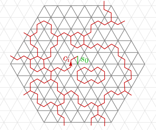
Figure 10: The graphical representation of a string net $\alpha\in\mathcal{P}_{n}^{C;i}$. The orientations and labels of the red strings are not shown, except for the piece that ensures that the constraint $B_{{s_{0}}}^{c_{i}}\ket{\alpha}=\ket{\alpha}$ is satisfied.

Lemma 4.7.

We have

$$\mathcal{W}^{C;i}_{n}=\textup{span}\{{\ket{\alpha}\,:\,\alpha\in\mathcal{P}_{n}^{C;i}}\}.$$

Proof.

That $\ket{\alpha}\in\mathcal{W}^{C;i}_{n}$ if $\alpha\in\mathcal{P}_{n}^{C;i}$ is immediate from the definitions. Conversely, since $\{B_{f}\}_{f\in{\overline{\Gamma}}^{F}_{n}}\cup\{B_{s_{0}}^{c_{i}}\}$ is a set of commuting projectors we have

$$\mathcal{W}^{C;i}_{n}=\left(\prod_{f\in{\overline{\Gamma}}^{F}_{n}}B_{f}\right)\,B_{s_{0}}^{c_{i}}\,\mathcal{H}_{n}.$$

Now note that the vectors $\ket{\alpha}$ for $\alpha\in\mathfrak{G}_{n}$ from an orthonormal basis for $\mathcal{H}_{n}$ and that

$$\left(\prod_{f\in{\overline{\Gamma}}^{F}_{n}}B_{f}\right)\,B_{s_{0}}^{c_{i}}\ket{\alpha}=\begin{cases}\ket{\alpha}\quad&\text{if }\,\,\,\alpha\in\mathcal{P}_{n}^{C;i}\\ 0&\text{otherwise}.\end{cases}$$

The claim follows. ∎

We can further refine the spaces $\mathcal{W}^{C;i}_{n}$ by specifying boundary conditions.

Definition 4.8.

We say a boundary condition $b\in\mathfrak{B}_{n}$ is compatible with the conjugacy class $C$ if $\phi_{\beta_{n}}(b)\in C$. We denote by $\mathfrak{B}_{n}^{C}$ the set of boundary conditions compatible with $C$. For $b\in\mathfrak{B}_{n}^{C}$ we have $\phi_{\beta_{n}}(b)=c_{i}\in C$ for a definite index $i\in\{1,\cdots,\absolutevalue{C}\}$. We write $i=i(b)$.

Definition 4.9.

For any conjugacy class $C\in(G)_{cj}$, any $i=1,\cdots,\absolutevalue{C}$, and any boundary condition $b\in\mathfrak{B}_{n}$ we let $\mathcal{W}_{n}^{C;ib}\subset\mathcal{H}_{n}$ be the space of vectors $\ket{\psi}\in\mathcal{H}_{n}$ that satisfy

$$\ket{\psi}=B_{f}\ket{\psi}=B_{{s_{0}}}^{c_{i}}\ket{\psi}=P_{b}\ket{\psi}$$

for all $f\in{\overline{\Gamma}}^{F}_{n}$. Here $P_{b}$ is the projector on the boundary condition $b$ form Definition 3.2.

Definition 4.10.

For any boundary condition $b\in\mathfrak{B}_{n}$ we let

$$\mathcal{P}_{n}^{C;ib}:=\{\alpha\in\mathcal{P}_{n}^{C;i}\,:\,b(\alpha)=b\}.$$

Lemma 4.11.

We have

$$\mathcal{W}_{n}^{C;ib}:=\textup{span}\{{\ket{\alpha}\,:\,\alpha\in\mathcal{P}_{n}^{C;ib}}\}.$$

Proof.

This follows from $\mathcal{W}^{C;i}_{n}=\textup{span}\{{\ket{\alpha}\,:\,\alpha\in\mathcal{P}_{n}^{C;i}}\}$ (Lemma 4.7), the fact that $\alpha\in\mathcal{P}_{n}^{C;ib}$ if and only if $\alpha\in\mathcal{P}_{n}^{C;i}$ and $P_{b}\ket{\alpha}=\ket{\alpha}$, and the fact (Lemma 4.4) that $\{B_{f}\}_{f\in{\overline{\Gamma}}^{F}_{n}}\cup\{B_{{s_{0}}}^{c_{i}},\,P_{b}\}$ is a set of commuting projectors. ∎

Lemma 4.12.

We have a disjoint union

$$\mathcal{P}_{n}^{C;i}=\bigsqcup_{b\in\mathfrak{B}_{n}^{C}}\mathcal{P}_{n}^{C;ib}$$

and an orthogonal decomposition

$$\mathcal{W}^{C;i}_{n}=\bigoplus_{b\in\mathfrak{B}_{n}^{C}}\mathcal{W}_{n}^{C;ib}.$$

In particular, $\mathcal{P}_{n}^{C;ib}$ is empty if $b$ is not compatible with $C$.

Proof.

To show the first claim, it is sufficient to show that $\mathcal{P}_{n}^{C;ib}$ is empty if $b$ is not compatible with $C$. This follows from Lemma B.3. The second claim then follows immediately from Lemma 4.11 and Lemma 4.7. ∎

4.3 Fiducial flux

The fiducial flux, which is measured by the projectors $T_{{\nu_{n}}}^{g}$, remains unconstrained by the projectors defining the spaces $\mathcal{W}_{n}^{C;ib}$, we can therefore further decompose the spaces $\mathcal{W}_{n}^{C;ib}$ according to the fiducial flux.

Lemma 4.13.

For any $C\in(G)_{cj}$, any $i=1,\cdots,\absolutevalue{C}$, any $g\in G$, and any boundary condition $b\in\mathfrak{B}_{n}$, the set

$$\{B_{f}\}_{f\in{\overline{\Gamma}}^{F}_{n}}\cup\{A_{v}\}_{v\in{\overline{\Gamma}}^{V}_{n}}\cup\{B_{{s_{0}}}^{c_{i}},\,P_{b},\,T_{{\nu_{n}}}^{g}\}$$

is a set of commuting projectors.

Proof.

That

$$\{B_{f}\}_{f\in{\overline{\Gamma}}^{F}_{n}}\cup\{A_{v}\}_{v\in{\overline{\Gamma}}^{V}_{n}}\cup\{B_{{s_{0}}}^{c_{i}},\,P_{b}\}$$

is a set of commuting projectors follows from Lemma 4.4. To prove the lemma, we must show that $T_{{\nu_{n}}}^{g}$ commutes with all the projectors in this set. From Lemma A.3 we get that $T_{{\nu_{n}}}^{g}$ commutes with all $A_{v}$ for $v\in{\overline{\Gamma}}^{V}_{n}$, all $B_{f}$ for $f\in{\overline{\Gamma}}^{F}_{n}$ and with $B_{{s_{0}}}^{c_{i}}$. To see that $T_{{\nu_{n}}}^{g}$ commutes with $P_{b}$, simply note that $P_{b}$ is supported on $\partial{\Gamma}^{E}_{n}$ while $T_{{\nu_{n}}}^{g}$ is supported on the ribbon ${\nu_{n}}$, whose support does not contain any edges of $\partial{\Gamma}^{E}_{n}$. ∎

Note that by Lemma B.4 we have for any $\alpha\in\mathcal{P}_{n}^{C;ib}$ that $\bar{q}_{i}\phi_{{\nu_{n}}}(\alpha)q_{i(b)}\in N_{C}$. This motivates the following Definition.

Definition 4.14.

For any conjugacy class $C\in(G)_{cj}$, any $i=1,\cdots,\absolutevalue{C}$, any boundary condition $b\in\mathfrak{B}_{n}$, and any $m\in N_{C}$ we let $\mathcal{W}_{n}^{C;ib}(m)\subset\mathcal{H}_{n}$ be the space of vectors $\ket{\psi}\in\mathcal{H}_{n}$ that satisfy

$$\ket{\psi}=B_{f}\ket{\psi}=B_{{s_{0}}}^{c_{i}}\ket{\psi}=P_{b}\ket{\psi}=T_{{\nu_{n}}}^{q_{i}m\bar{q}_{i(b)}}\ket{\psi}$$

for all $f\in{\overline{\Gamma}}^{F}_{n}$.

These spaces are again spanned by certain string-net states that have a definite fiducial flux.

Definition 4.15.

For any $m\in N_{C}$ we define

$$\mathcal{P}_{n}^{C;ib}(m):=\{\alpha\in\mathcal{P}_{n}^{C;ib}\,:\,\phi_{{\nu_{n}}}(\alpha)=q_{i}m\bar{q}_{i(b)}\}.$$

Lemma 4.16.

We have

$$\mathcal{W}_{n}^{C;ib}(m)=\textup{span}\{{\ket{\alpha}\,:\,\alpha\in\mathcal{P}_{n}^{C;ib}(m)}\}.$$

Proof.

This follows from Lemma 4.13 and the fact that

$$T_{{\nu_{n}}}^{g}\ket{\alpha}=\delta_{\phi_{{\nu_{n}}}(\alpha),g}\ket{\alpha},$$

see Lemma B.11. ∎

Lemma 4.17.

We have a disjoint union

$$\mathcal{P}_{n}^{C;ib}=\bigsqcup_{m\in N_{C}}\,\mathcal{P}_{n}^{C;ib}(m)$$

and an orthogonal decomposition

$$\mathcal{W}_{n}^{C;ib}=\bigoplus_{m\in N_{C}}\,\mathcal{W}_{n}^{C;ib}(m).$$

Proof.

For the first claim it suffices to note that for any $\alpha\in\mathcal{P}_{n}^{C;ib}$ we have $\bar{q}_{i}\phi_{{\nu_{n}}}(\alpha)q_{i(b)}\in N_{C}$. This is the content of Lemma B.4. The second claim follows immediately from the first and Lemmas 4.11 and 4.13. ∎

4.4 Imposing gauge invariance on ${\overline{\Gamma}}^{V}_{n}$

Definition 4.18.

For any conjugacy class $C$, any $i=1,\cdots,\absolutevalue{C}$, any boundary condition $b\in\mathfrak{B}_{n}^{C}$, and any $m\in N_{C}$ we define $\mathcal{V}_{n}^{C;ib}(m)\subset\mathcal{H}_{n}$ to be the space of vectors $\ket{\psi}\in\mathcal{H}_{n}$ that satisfy

$$\ket{\psi}=B_{f}\ket{\psi}=B_{{s_{0}}}^{c_{i}}\ket{\psi}=P_{b}\ket{\psi}=T_{{\nu_{n}}}^{q_{i}m\bar{q}_{i(b)}}\ket{\psi}=A_{v}\ket{\psi}$$

for all $f\in{\overline{\Gamma}}^{F}_{n}$ and all $v\in{\overline{\Gamma}}^{V}_{n}$.

We will show that the spaces $\mathcal{V}_{n}^{C;ib}(m)$ are one-dimensional. To this end we introduce the following group of gauge transformations.

Definition 4.19.

We let $\overline{\mathcal{G}}_{n}:=\mathcal{G}_{{\overline{\Gamma}}^{V}_{n}}$ be the group of gauge transformations on ${\overline{\Gamma}}^{V}_{n}$. All of its elements are unitaries of the form

$$U[\{g_{v}\}]=\prod_{v\in{\overline{\Gamma}}^{V}_{n}}\,A_{v}^{g_{v}}$$

for some $\{g_{v}\}\in G^{|{\overline{\Gamma}}^{V}_{n}|}$.

Let us note that the average over this gauge group is

$$\frac{1}{\absolutevalue{\overline{\mathcal{G}}_{n}}}\,\sum_{U\in\overline{\mathcal{G}}_{n}}U=\frac{1}{\absolutevalue{G}^{\absolutevalue{{\overline{\Gamma}}^{V}_{n}}}}\sum_{\{g_{v}\}\in G^{|{\overline{\Gamma}}^{V}_{n}|}}\,\prod_{v\in{\overline{\Gamma}}^{V}_{n}}A_{v}^{g_{v}}=\prod_{v\in{\overline{\Gamma}}^{V}_{n}}\,\left(\frac{1}{\absolutevalue{G}}\,\sum_{g_{v}\in G}A_{v}^{g_{v}}\right)=\prod_{v\in{\overline{\Gamma}}^{V}_{n}}A_{v}.$$

Lemma 4.20.

We have

$$\mathcal{V}_{n}^{C;ib}(m)=\left(\frac{1}{\absolutevalue{\overline{\mathcal{G}}_{n}}}\sum_{U\in\overline{\mathcal{G}}_{n}}U\right)\,\mathcal{W}_{n}^{C;ib}(m).$$

Proof.

Since $\frac{1}{\absolutevalue{\overline{\mathcal{G}}_{n}}}\sum_{U\in\overline{\mathcal{G}}_{n}}U=\prod_{v\in{\overline{\Gamma}}^{V}_{n}}A_{v}$, it is sufficient to show that

$$\mathcal{V}_{n}^{C;ib}(m)=\bigg{(}\prod_{v\in{\overline{\Gamma}}^{V}_{n}}A_{v}\bigg{)}\,\mathcal{W}_{n}^{C;ib}(m).$$

This follows immediately from the Definition 4.14 and Lemma 4.13. ∎

We now define unit vectors which, as we shall see, span the spaces $\mathcal{V}_{n}^{C;ib}(m)$.

Definition 4.21.

For all $n>1$, all conjugacy classes $C\in(G)_{cj}$, all labels $i=1,\cdots,\absolutevalue{C}$, all boundary conditions $b\in\mathfrak{B}_{n}^{C}$, and all $m\in N_{C}$ we define the unit vector

$$\ket{\eta_{n}^{C;ib}(m)}:=\frac{1}{\absolutevalue{\mathcal{P}_{n}^{C;ib}(m)}^{1/2}}\,\sum_{\alpha\in\mathcal{P}_{n}^{C;ib}(m)}\,\ket{\alpha}.$$

We can now use the fact that $\mathcal{W}_{n}^{C;ib}(m)$ is spanned by vectors $\ket{\alpha}$ with $\alpha\in\mathcal{P}_{n}^{C;ib}(m)$ and that the gauge group $\overline{\mathcal{G}}_{n}$ acts freely and transitively on $\mathcal{P}_{n}^{C;ib}(m)$ to show

Lemma 4.22.

The space $\mathcal{V}_{n}^{C;ib}(m)\subset\mathcal{H}_{n}$ is one-dimensional and spanned by the vector $\ket{\eta_{n}^{C;ib}(m)}$. In particular, the vectors $\biggl{\{}\ket{\eta_{n}^{C;ib}(m)}\bigg{\}}_{C,i,b,m}$ form an orthonormal family.

Proof.

By Lemma 4.16, we have $\mathcal{W}_{n}^{C;ib}(m)=\textup{span}\{{\ket{\alpha}\,:\,\alpha\in\mathcal{P}_{n}^{C;ib}(m)}\}$. By Lemma 4.20 it is sufficient to show that

$$\sum_{U\in\overline{\mathcal{G}}_{n}}U\ket{\alpha}\propto\ket{\eta_{n}^{C;ib}(m)}$$

for all $\alpha\in\mathcal{P}_{n}^{C;ib}(m)$. This follows immediately from Lemma B.10 which states that $\overline{\mathcal{G}}_{n}$ acts freely and transitively on $\mathcal{P}_{n}^{C;ib}(m)$:

$$\sum_{U\in\overline{\mathcal{G}}_{n}}U\ket{\alpha}=\sum_{\alpha^{\prime}\in\mathcal{P}_{n}^{C;ib}(m)}\ket{\alpha^{\prime}}=\absolutevalue{\mathcal{P}_{n}^{C;ib}(m)}^{1/2}\ket{\eta_{n}^{C;ib(m)}}.$$

∎

4.5 Action of $N_{C}$ on fiducial flux and irreducible subspaces

The gauge transformations $A_{v_{0}}^{q_{i}m\bar{q}_{i}}$ realise a left group action of $N_{C}$ on the vectors $\ket{\eta_{n}^{C;ib}(m)}$.

Lemma 4.23.

For any $m_{1},m_{2}\in N_{C}$ we have

$$A_{{s_{0}}}^{q_{i}m_{1}\bar{q}_{i}}\ket{\eta_{n}^{C;ib}(m_{2})}=\ket{\eta_{n}^{C;ib}(m_{1}m_{2})}.$$

Proof.

If $\alpha\in\mathcal{P}_{n}^{C;ib}(m_{2})$, then by definition $\phi_{{\nu_{n}}}(\alpha)=q_{i}m_{2}\bar{q}_{i(b)}$. The gauge transformation $A_{{s_{0}}}^{q_{i}m_{1}\bar{q}_{i}}$ acts on such a string-net to yield $\ket{\alpha^{\prime}}=A_{{s_{0}}}^{q_{i}m_{1}\bar{q}_{i}}\ket{\alpha}$ for a new string net $\alpha^{\prime}$. Since $A_{{s_{0}}}^{q_{i}m_{1}\bar{q}_{i}}$ commutes with the projectors $\{B_{{s_{0}}}^{c_{i}},P_{b}\}\cup\{B_{f}\}_{f\in{\overline{\Gamma}}^{F}_{n}}$ (Lemma 4.4) and we have $\phi_{{\nu_{n}}}(\alpha^{\prime})=q_{i}m_{1}m_{2}\bar{q}_{i}$ by Lemma A.3, we find that $\alpha^{\prime}\in\mathcal{P}_{n}^{C;ib}(m_{1}m_{2})$. Since $A_{{s_{0}}}^{q_{i}m_{2}\bar{q}_{i}}$ acts invertibly on string nets, we see that it yields a bijection from $\mathcal{P}_{n}^{C;ib}(m_{1})$ to $\mathcal{P}_{n}^{C;ib}(m_{1}m_{2})$. In particular, these sets have the same cardinality and

$$A_{{s_{0}}}^{q_{i}m_{1}\bar{q}_{i}}\ket{\eta_{n}^{C;ib}(m_{2})} =\frac{1}{\absolutevalue{\mathcal{P}_{n}^{C;ib}(m_{2})}^{1/2}}\sum_{\alpha\in\mathcal{P}_{n}^{C;ib}(m_{2})}\,{q_{i}m_{1}\bar{q}_{i}}\ket{\alpha}$$

$$=\frac{1}{\absolutevalue{\mathcal{P}_{n}^{C;ib}(m_{1}m_{2})}^{1/2}}\sum_{\alpha\in\mathcal{P}_{n}^{C;ib}(m_{1}m_{2})}\,\ket{\alpha}$$

$$=\ket{\eta_{n}^{C;ib}(m_{1}m_{2})}.$$

∎

The space spanned by the vectors $\Bigl{\{}\ket{\eta_{n}^{C;ib}(m)}\Bigl{\}}_{m\in N_{C}}$ therefore carries the regular representation of $N_{C}$, with a left group action provided by the gauge transformations $A_{{s_{0}}}^{q_{i}m\bar{q}_{i}}$ for $m\in N_{C}$, which are supported near the site ${s_{0}}$. It turns out that this space also carries a natural right action of $N_{C}$ provided by unitaries supported near the boundary of ${\Gamma}^{E}_{n}$, see Lemma B.17.

We can characterise this space as follows. Let us define

Definition 4.24.

$\mathcal{V}_{n}^{C;ib}\subset\mathcal{H}_{n}$ is the subspace consisting of vectors $\ket{\psi}\in\mathcal{H}_{n}$ such that

$$\ket{\psi}=A_{v}\ket{\psi}=B_{f}\ket{\psi}=B_{{s_{0}}}^{c_{i}}\ket{\psi}=P_{b}\ket{\psi}$$

for all $v\in{\overline{\Gamma}}^{V}_{n}$ and all $f\in{\overline{\Gamma}}^{F}_{n}$.

Then

Lemma 4.25.

$$\mathcal{V}_{n}^{C;ib}=\bigoplus_{m\in N_{C}}\,\mathcal{V}_{n}^{C;ib}(m)=\textup{span}\{{\ket{\eta_{n}^{C;ib}(m)}\,:\,m\in N_{C}}\}.$$

Proof.

The spaces $\mathcal{V}_{n}^{C;ib}(m)$ are defined by the same constraints as the space $\mathcal{V}_{n}^{C;ib}$, plus the constraint $T_{{\nu_{n}}}^{q_{i}m\bar{q}_{i(b)}}$ on the fiducial flux (Definitions 4.18 and 4.24).

Since $\mathcal{V}_{n}^{C;ib}\subset\mathcal{W}_{n}^{C;ib}$ (cf. Definition 4.9) is spanned by vectors $\ket{\alpha}$ for $\alpha\in\mathcal{P}_{n}^{C;ib}$ (Lemma 4.11) which satisfy $q_{i}\phi_{{\nu_{n}}}(\alpha)\bar{q}_{i(b)}\in N_{C}$ (Lemma B.4), we have (using Lemma B.11) $\sum_{m\in N_{C}}T_{{\nu_{n}}}^{q_{i}m\bar{q}_{i(b)}}\,\ket{\phi}=\ket{\phi}$ for all $\ket{\phi}\in\mathcal{V}_{n}^{C;ib}$.

Using Lemma 4.13, it follows that

$$\mathcal{V}_{n}^{RC;ib}=\sum_{m\in N_{C}}\,T_{{\nu_{n}}}^{q_{i}m\bar{q}_{{i(b)}}}\,\mathcal{V}_{n}^{C;ib}=\bigoplus_{m\in N_{C}}\,\mathcal{V}_{n}^{C;ib}(m)$$

as required.

The second equality in the claim now follows immediately from Lemma 4.22. ∎

Since $\mathcal{V}_{n}^{C;ib}$ carries the regular representation of $N_{C}$, we can construct an orthonormal basis of $\mathcal{V}_{n}^{C;ib}$ that respects the irreducible subspaces of $\mathcal{V}_{n}^{C;ib}$ for both the left and the right action of $N_{C}$.

Definition 4.26.

For any conjugacy class $C\in(G)_{cj}$, any irreducible representation $R\in(N_{C})_{irr}$, any label $u=(i,j)\in I_{RC}$, any boundary condition $b\in\mathfrak{B}_{n}^{C}$, and any label $j^{\prime}=1,\cdots,\mathrm{dim}R$, and writing $v=(b,j^{\prime})$, we define a vector

$$\ket{\eta_{n}^{RC;uv}}:=\left(\frac{\mathrm{dim}R}{\absolutevalue{N_{C}}}\right)^{1/2}\,\sum_{m\in N_{C}}\,R^{jj^{\prime}}(m)^{*}\ket{\eta_{n}^{C;ib}(m)}.$$

We will write $I^{\prime}_{RC}:=\mathfrak{B}_{n}^{C}\times\{1,\cdots,\mathrm{dim}R\}$ for the possible values of the label $v=(b,j^{\prime})$.

Lemma 4.27.

The vectors $\{\ket{\eta_{n}^{RC;uv}}\}$ form an orthonormal basis, i.e.

$$\langle{\eta_{n}^{R_{1}C_{1};u_{1}v_{1}}},{\eta_{n}^{R_{2}C_{2};u_{2}v_{2}}}\rangle=\delta_{R_{1}C_{1},R_{2}C_{2}}\delta_{u_{1},u_{2}}\delta_{v_{1},v_{2}}.$$

Proof.

Let $u_{1}=(i_{1},j_{1})$, $u_{2}=(i_{2},j_{2})$, $v_{1}=(b_{1},j^{\prime}_{1})$ and $v_{2}=(b_{2},j^{\prime}_{2})$. Then

$$\langle{\eta_{n}^{R_{1}C_{1};u_{1}v_{1}}},{\eta_{n}^{R_{2}C_{2};u_{2}v_{2}}}\rangle=\frac{(\dim(R_{1})\dim(R_{2}))^{1/2}}{\absolutevalue{N_{C_{1}}}}\,\delta_{C_{1},C_{2}}\,\delta_{i_{1},i_{2}}\delta_{b_{1},b_{2}}\,\sum_{m\in N_{C_{1}}}\,R^{j_{1}j^{\prime}_{1}}(m)\,R^{j_{2}j^{\prime}_{2}}(m)^{*}$$

where we used that the vectors $\ket{\eta_{n}^{C;ib}(m)}$ are orthonormal (Lemma 4.22). Now using the Schur orthogonality relation (19) gives us the required result. ∎

The $\ket{\eta_{n}^{RC;uv}}$ were in fact obtained by a unitary rotation of the states $\ket{\eta_{n}^{C;ib}(m)}$, and this rotation can be reversed.

Lemma 4.28.

We have for all $C\in(G)_{cj}$, all $i=1,\cdots,\absolutevalue{C}$, all $b\in\mathfrak{B}_{n}^{C}$, and all $m\in N_{C}$ that

$$\ket{\eta_{n}^{C;ib}(m)}=\sum_{R\in(N_{C})_{irr}}\,\frac{\mathrm{dim}R}{\absolutevalue{N_{C}}}\,\sum_{j,j^{\prime}}\,R^{jj^{\prime}}(m)\,\ket{\eta_{n}^{RC;(i,j)(b,j^{\prime})}}.$$

Proof.

We have

$$\sum_{R\in(N_{C})_{irr}}\, \frac{\mathrm{dim}R}{\absolutevalue{N_{C}}}\,\sum_{j,j^{\prime}}\,R^{jj^{\prime}}(m)\,\ket{\eta_{n}^{RC;(i,j)(b,j^{\prime})}}$$

$$=\sum_{R\in(N_{C})_{irr}}\,\frac{\mathrm{dim}R}{\absolutevalue{N_{C}}}\,\sum_{j,j^{\prime}}\,\sum_{m^{\prime}\in N_{C}}\,R^{jj^{\prime}}(m)R^{jj^{\prime}}(m^{\prime})^{*}\,\ket{\eta_{n}^{C;ib}(m^{\prime})}$$

$$=\,\sum_{R\in(N_{C})_{irr}}\,\frac{1}{\absolutevalue{N_{C}}}\sum_{m^{\prime}\in N_{C}}\,\chi_{R}(m\bar{m}^{\prime})\chi_{R}(1)^{*}\,\ket{\eta_{n}^{C;ib}(m^{\prime})}$$

$$=\ket{\eta_{n}^{C;ib}(m)}$$

where we used $\chi_{R}(1)=\mathrm{dim}R$ and the Schur orthogonality relation (20) for irreducible characters. ∎

4.6 Characterisation of the spaces $\overline{\mathcal{V}_{n}}$, $\mathcal{V}_{n}^{RC}$, and $\mathcal{V}_{n}^{RC;u}$

We can now describe the spaces $\overline{\mathcal{V}_{n}},\mathcal{V}_{n}^{RC}$ and $\mathcal{V}_{n}^{RC;u}$ from Definition 4.3 in terms of the vectors $\ket{\eta_{n}^{RC;uv}}$.

Proposition 4.29.

We have

$$\overline{\mathcal{V}_{n}} =\textup{span}\{{\ket{\eta_{n}^{RC;uv}}\,:\,C\in(G)_{cj},R\in(N_{C})_{irr},u\in I_{RC},v\in I^{\prime}_{RC}}\},$$

$$\mathcal{V}_{n}^{RC} =\textup{span}\{{\ket{\eta_{n}^{RC;uv}}\,:\,u\in I_{RC},v\in I^{\prime}_{RC}}\},$$

$$\mathcal{V}_{n}^{RC;u} =\textup{span}\{{\ket{\eta_{n}^{RC;uv}}\,:\,v\in I^{\prime}_{RC}}\}.$$

Proof.

We first note that it follows from Lemma 4.12, Definition 4.9, and Lemma 4.4 that

$$B_{{s_{0}}}^{c_{i}}\bigg{(}\prod_{f\in{\overline{\Gamma}}^{F}_{n}}B_{f}\bigg{)}\,P_{b}=0$$

whenever $b\in\mathfrak{B}_{n}$ is not compatible with $C$. Using this, the fact that $\sum_{C,i}B_{{s_{0}}}^{c_{i}}=\sum_{b\in\mathfrak{B}_{n}}P_{b}=\mathds{1}$, and Lemma 4.4 we find

$$\overline{\mathcal{V}_{n}} =\bigg{(}\prod_{v\in{\overline{\Gamma}}^{V}_{n}}A_{v}\prod_{f\in{\overline{\Gamma}}^{F}_{n}}B_{f}\bigg{)}\,\mathcal{H}_{n}=\sum_{C\in(G)_{cj}}\sum_{i=1}^{\absolutevalue{C}}\sum_{b\in\mathfrak{B}_{n}}\bigg{(}\prod_{v\in{\overline{\Gamma}}^{V}_{n}}A_{v}\bigg{)}\,B_{{s_{0}}}^{c_{i}}\bigg{(}\prod_{f\in{\overline{\Gamma}}^{F}_{n}}B_{f}\bigg{)}\,P_{b}\,\mathcal{H}_{n}$$

$$=\sum_{C\in(G)_{cj}}\sum_{i=1}^{\absolutevalue{C}}\sum_{b\in\mathfrak{B}_{n}^{C}}\,\bigg{(}\prod_{v\in{\overline{\Gamma}}^{V}_{n}}A_{v}\bigg{)}\,B_{{s_{0}}}^{c_{i}}\bigg{(}\prod_{f\in{\overline{\Gamma}}^{F}_{n}}B_{f}\bigg{)}\,P_{b}\,\mathcal{H}_{n}$$

$$=\bigoplus_{C\in(G)_{cj}}\bigoplus_{i=1}^{\absolutevalue{C}}\bigoplus_{b\in\mathfrak{B}_{n}^{C}}\,\mathcal{V}_{n}^{C;ib},$$

where we used the Definition 4.24 of the spaces $\mathcal{V}_{n}^{C;ib}$. From Lemma 4.25 it then follows that

$$\overline{\mathcal{V}_{n}}=\textup{span}\{{\ket{\eta_{n}^{C;ib}(m)}\,:\,C\in(G)_{cj},i=1,\cdots,\absolutevalue{C},b\in\mathfrak{B}_{n}^{C},m\in N_{C}}\}.$$

Together with Definition 4.26 and Lemma 4.28 this yield the first claim.

To show the second claim we note that $\mathcal{V}_{n}^{RC}=D_{{s_{0}}}^{RC}\overline{\mathcal{V}_{n}}$, and for any $C_{1},C_{2}\in(G)_{cj}$, $R_{1}\in(N_{C_{1}})_{irr}$, $R_{2}\in(N_{C_{2}})_{irr}$, $u=(i,j)\in I_{R_{2}C_{2}}$, and $v=(b,j^{\prime})\in I^{\prime}_{R_{2}C_{2}}$ we have (Lemma B.15)

$$D_{{s_{0}}}^{R_{1}C_{1}}\ket{\eta_{n}^{R_{2}C_{2};uv}}=\delta_{R_{1}C_{1},R_{2}C_{2}}\,\ket{\eta_{n}^{R_{2}C_{2};uv}}.$$

The second claim of the Proposition then follows from the fact that $\overline{\mathcal{V}_{n}}$ is spanned by the vectors $\ket{\eta_{n}^{RC;uv}}$ for arbitrary $RC$ and $u\in I_{RC}$, $v\in I^{\prime}_{RC}$.

To show the final claim we note that we have $\mathcal{V}_{n}^{RC;u}=D_{{s_{0}}}^{RC;u}\mathcal{V}_{n}^{RC}$, and for any $u_{1},u_{2}\in I_{RC}$ and any $v\in I^{\prime}_{RC}$ we have (Lemma B.16)

$$D_{{s_{0}}}^{RC;u_{1}}\,\ket{\eta_{n}^{RC;u_{2}v}}=\delta_{u_{1},u_{2}}\,\ket{\eta_{n}^{RC;u_{2}v}}.$$

The final claim then follows from the fact that $\mathcal{V}_{n}^{RC}$ is spanned by the vectors $\ket{\eta_{n}^{RC;uv}}$ for $u\in I_{RC}$ and $v\in I^{\prime}_{RC}$. ∎

4.7 The bulk is independent of boundary conditions

Let us define the following operators

Definition 4.30.

For any site $s$, any $n$, any $u_{1}=(i_{1},j_{1}),u_{2}=(i_{2},j_{2})\in I_{RC}$, and any $v_{1}=(b_{1},j_{1}^{\prime}),v_{2}=(b_{2},j_{2}^{\prime})\in I^{\prime}_{RC}$ we define

$$a_{s}^{RC;u_{2}u_{1}} :=\frac{\mathrm{dim}R}{|N_{C}|}\sum_{m\in N_{C}}R^{j_{2}j_{1}}(m)^{*}A_{s}^{q_{i_{2}}m\overline{q}_{i_{1}}},$$

$$\tilde{a}_{n}^{RC;v_{2}v_{1}} :=\frac{\mathrm{dim}R}{|N_{C}|}\sum_{m\in N_{C}}R^{j^{\prime}_{2}j^{\prime}_{1}}(m)U_{b_{2}b_{1}}L_{\beta_{n}}^{{q_{i(b_{1})}\overline{m}\,\overline{q}_{i(b_{1})}}}$$

where $\beta_{n}$ is the boundary ribbon and $U_{b_{2}b_{1}}$ is a boundary unitary provided by Lemma B.9 which we choose such that $U_{b_{2}b_{1}}=U_{b_{1}b_{2}}^{*}$. These boundary unitaries satisfy the following: for any $\alpha\in\mathcal{P}_{n}^{C;ib_{1}}$ we have $U_{b_{2}b_{1}}\ket{\alpha}=\ket{\alpha^{\prime}}$ where $\alpha^{\prime}\in\mathcal{P}_{n}^{C;ib_{2}}$, and $\alpha^{\prime}_{e}=\alpha_{e}$ for all $e\in{\Gamma}^{E}_{n-1}$ and $b(\alpha^{\prime})=b_{2}$.

Note that the $\tilde{a}_{n}^{RC;v_{2}v_{1}}$ are supported on ${\Gamma}^{E}_{n}\setminus{\Gamma}^{E}_{n-1}$ and $a_{{s_{0}}}^{RC;u_{2}u_{1}}$ is supported on ${\Gamma}^{E}_{1}$. From Lemma B.18 we have for any $u,u_{1},u_{2}\in I_{RC}$ and any $v,v_{1},v_{2}\in I^{\prime}_{RC}$ that

$$a_{{s_{0}}}^{RC;u_{2}u_{1}}\ket{\eta_{n}^{RC;u_{1}v}}=\ket{\eta_{n}^{RC;u_{2}v}},\quad\quad\tilde{a}_{n}^{RC;v_{2}v_{1}}\ket{\eta_{n}^{RC;uv_{1}}}=\ket{\eta_{n}^{RC;u,v_{2}}}$$

as well as

$$(a_{{s_{0}}}^{RC;u_{1}u_{2}})^{*}\ket{\eta_{n}^{RC;u_{1}v}}=\ket{\eta_{n}^{RC;u_{2}v}},\quad\quad(\tilde{a}_{n}^{RC;v_{1}v_{2}})^{*}\ket{\eta_{n}^{RC;uv_{1}}}=\ket{\eta_{n}^{RC;u,v_{2}}}$$

i.e. these operators change the labels $u$ and $v$ when acting on the states $\ket{\eta_{n}^{RC;uv}}$. We can use these ‘label changers’ to show that expectation values of operators supported on ${\Gamma}^{E}_{n-1}$ in the state $\ket{\eta_{n}^{RC;uv}}$ are independent of the boundary label $v$.

Lemma 4.31.

$\langle{{\eta_{n}^{RC;uv}}},{O\,{\eta_{n}^{RC;uv}}}\rangle$ is independent of $v$ for all $O\in\mathfrak{A}_{{\Gamma}^{E}_{n-1}}$

Proof.

Using Lemma B.18 and the fact that any $O\in\mathfrak{A}_{{\Gamma}^{E}_{n-1}}$ commutes with $\tilde{a}_{n}^{RC;vv^{\prime}}$ we find

$$\langle{{\eta_{n}^{RC;uv}}},{O{\eta_{n}^{RC;uv}}}\rangle=\langle{{\eta_{n}^{RC;uv^{\prime}}}},{O\,(\tilde{a}_{n}^{RC;vv^{\prime}})^{*}\tilde{a}_{n}^{RC;vv^{\prime}}{\eta_{n}^{RC;uv^{\prime}}}}\rangle.$$

∎

This Lemma shows that the following is well-defined.

Definition 4.32.

For any $n$ we define the states ${\eta_{n}^{RC;u}}$ on $\mathfrak{A}_{{\Gamma}^{E}_{n}}$ by

$${\eta_{n}^{RC;u}}(O):=\langle{\eta_{n+1}^{RC;uv}},{O\,\eta_{n+1}^{RC;uv}}\rangle$$

for any $O\in\mathfrak{A}_{{\Gamma}^{E}_{n}}$ and any boundary label $v$. The choice of boundary label does not matter due to Lemma 4.31.

4.8 Construction of the states $\omega^{RC;u}_{{s_{0}}}$ and proof of their purity

Let us define the following sets of states on $\mathfrak{A}_{{\Gamma}^{E}_{n}}$.

Definition 4.33.

The set $\mathcal{S}_{n}^{RC;u}$ consists of states $\omega$ on $\mathfrak{A}_{{\Gamma}^{E}_{n}}$ such that

$$1=\omega(D_{{s_{0}}}^{RC;u})=\omega(A_{v})=\omega(B_{f})$$

for all $v\in{\overline{\Gamma}}^{V}_{n}$ and all $f\in{\overline{\Gamma}}^{F}_{n}$.

Lemma 4.34.

Let $1\leq m<n$. If $\omega\in\mathcal{S}_{n}^{RC;u}$, and $\omega_{m}$ is its restriction to $\mathfrak{A}_{{\Gamma}^{E}_{m}}$, then $\omega_{m}={\eta_{m}^{RC;u}}$.

Proof.

Let $\omega_{m+1}$ be the restriction of $\omega$ to $\mathfrak{A}_{{\Gamma}^{E}_{m+1}}$, then $\omega_{m+1}\in\mathcal{S}_{m+1}^{RC;u}$. Let $\omega_{m+1}=\sum_{\kappa}\lambda_{\kappa}\omega_{m+1}^{(\kappa)}$ be the convex decomposition of $\omega_{m+1}$ into finitely many pure components $\omega_{m+1}^{(\kappa)}$. Let $\ket{\Omega_{m+1}^{(\kappa)}}\in\mathcal{H}_{m+1}$ be unit vectors corresponding to these pure states. We conclude from Lemma 3.24 that

$$A_{v}\ket{\Omega_{m+1}^{(\kappa)}}=B_{f}\ket{\Omega_{m+1}^{(\kappa)}}=D_{s_{0}}^{RC;u}\ket{\Omega_{m+1}^{(\kappa)}}=\ket{\Omega_{m+1}^{(\kappa)}}$$

for all $\kappa$, all $v\in{\overline{\Gamma}}^{V}_{m+1}$, and all $f\in{\overline{\Gamma}}^{F}_{m+1}$. By Definition 4.3 this means that $\ket{\Omega_{m+1}^{(\kappa)}}\in\mathcal{V}_{m+1}^{RC;u}$ for all $\kappa$. From Proposition 4.29 it follows that the unit vectors $\ket{\Omega_{m+1}^{(\kappa)}}$ are linear combinations of the $|\eta_{m+1}^{RC;uv}\rangle$ for $v\in I^{\prime}_{RC}$, and using Lemmas B.18 and B.19 as well as Lemma 4.31 and Definition 4.32 we have for any $O\in{\Gamma}^{E}_{m}$ that

$$\omega_{m+1}^{(\kappa)}(O)=\langle{\Omega_{m+1}^{(\kappa)}},{O\,\Omega_{m+1}^{(\kappa)}}\rangle=\eta_{m}^{RC;u}(O),$$

independently of $\kappa$. The claim follows. ∎

We define extensions of the states ${\eta_{n}^{RC;u}}$ to the whole observable algebra.

Definition 4.35.

We let $\tilde{\eta}_{n}^{RC;u}$ be the following extension of ${\eta_{n}^{RC;u}}$ to the whole observable algebra. For each $e\in\Gamma^{E}$, let $\zeta_{e}$ be the pure state on $\mathfrak{A}_{e}$ corresponding to the vector $|1_{e}\rangle\in\mathcal{H}_{e}$, and put

$$\tilde{\eta}_{n}^{RC;u}:={\eta_{n}^{RC;u}}\otimes\left(\bigotimes_{e\in\Gamma^{E}\setminus{\Gamma}^{E}_{n}}\zeta_{e}\right).$$

Recall the space of states $\mathcal{S}_{s_{0}}^{RC;u}$ from Definition 4.2.

Lemma 4.36.

The sequence of states $\tilde{\eta}_{n}^{RC;u}$ converges in the weak-^∗ topology to a state $\omega^{RC;u}_{{s_{0}}}\in\mathcal{S}_{s_{0}}^{RC;u}$.

Proof.

If $O\in\mathfrak{A}_{{\Gamma}^{E}_{m}}$ then $\tilde{\eta}_{n}^{RC;u}(O)=\eta_{n}^{RC;u}(O)$ for all $n>m$ by construction. Since $\eta_{n}^{RC;u}\in\mathcal{S}_{n}^{RC;u}$ we have from Lemma 4.34 that $\tilde{\eta}_{n}^{RC;u}|_{m}={\eta_{m}^{RC;u}}$. It follows that $\tilde{\eta}_{n}^{RC;u}(O)$ is constant for all $n>m$ and hence converges. Since $m$ was chosen arbitrarily, $\tilde{\eta}_{n}^{RC;u}$ converges for any local observable $O\in\mathfrak{A}_{loc}$. Since $\mathfrak{A}_{loc}$ is dense in $\mathfrak{A}$, the states $\omega_{n}^{RC;u}$ converge in the weak-^∗ topology to some state $\omega^{RC;u}_{{s_{0}}}$ that satisfies the constraints (3) and $\eqref{eq:cons3}$, i.e. $\omega^{RC;u}_{{s_{0}}}\in\mathcal{S}_{{s_{0}}}^{RC;u}$. ∎

Lemma 4.37.

$\omega^{RC;u}_{{s_{0}}}$ is the unique state in $\mathcal{S}_{{s_{0}}}^{RC;u}$. It is therefore a pure state.

Proof.

Consider any other state $\omega^{\prime}\in\mathcal{S}_{{s_{0}}}^{RC;u}$. Then its restriction $\omega^{\prime}_{n}$ to $\mathfrak{A}_{{\Gamma}^{E}_{n}}$ is a state in $\mathcal{S}^{RC;u}_{n}$ and thus by Lemma 4.34 we have $\omega^{\prime}(O)=\omega^{\prime}_{n}(O)={\eta_{m}^{RC;u}}(O)=\omega_{n}^{RC;u}(O)$ for all $m<n$ and all $O\in\mathfrak{A}_{{\Gamma}^{E}_{m}}$. It follows that $\omega^{\prime}$ agrees with $\omega^{RC;u}_{{s_{0}}}$ on all local observables and therefore must be the same state. ∎

Since the site ${s_{0}}$ was arbitrary, we have in particular shown

Proposition 4.38.

For any site $s_{0}$, any irreducible representation $RC$ of $\mathcal{D}(G)$, and any label $u$, the space of states $\mathcal{S}_{s_{0}}^{RC;u}$ of Definition 4.2 consists of a single pure state $\omega_{s_{0}}^{RC;u}$.

5 Construction of anyon sectors

In this section we show that the pure states $\omega_{s_{1}}^{R_{1}C_{1};u_{1}},\omega_{s_{2}}^{R_{2}C_{2};u_{2}}$ constructed in the previous Section are equivalent to each other whenever $R_{1}C_{1}=R_{2}C_{2}$. The collection of pure states $\{\omega_{s}^{RC;u}\}_{s,u}$ for fixed $RC$ therefore belong to the same irreducible representation $\pi^{RC}$ of the observable algebra. We will show that the irreducible representations $\{\pi^{RC}\}_{RC}$ are pairwise disjoint. In other words, we show that the data $RC$ labels different superselection sectors. Finally, we will show that the representations $\pi^{RC}$ are anyon sectors by relating them to so-called amplimorphism representations [Naa15].

5.1 Ribbon operators and their limiting maps

From this point onward, the ribbon operators introduced in Section 3.1 will play an increasingly important role in the analysis. By taking certain linear combinations of these ribbon operators, we construct new ribbon operators that can produce, transport, and detect anyonic excitations above the frustration free ground state.

Recall from section 3.1 that we can associate to any finite ribbon $\rho$ some ribbon operators $F_{\rho}^{h,g}$.

Definition 5.1.

For each irreducible representation $RC$ of the quantum double we define

$$F^{RC;uv}_{\rho}:=\frac{\mathrm{dim}R}{|N_{C}|}\sum_{m\in N_{C}}{R}^{jj^{\prime}}(m)^{*}F^{\overline{c}_{i},q_{i}m\overline{q}_{i^{\prime}}}_{\rho}$$

where $u=(i,j)\in I_{RC}$ and $v=(i^{\prime},j^{\prime})\in I_{RC}$.

Definition 5.2.

For any finite ribbon $\rho$, any $RC$, and any $u_{1},u_{2}\in I_{RC}$ we define a linear map from $\mathfrak{A}$ to itself by

$$\mu^{RC;u_{1}u_{2}}_{\rho}(O):=\bigg{(}\frac{|N_{C}|}{\mathrm{dim}R}\bigg{)}^{2}\sum_{v}\,\big{(}F_{\rho}^{RC;u_{1}v}\big{)}^{*}\,O\,F_{\rho}^{RC;u_{2}v}$$

for any $O\in\mathfrak{A}$.

We define a half-infinite ribbon to be a sequence $\rho=\{\tau_{i}\}_{i\in\mathbb{N}}$ of triangles such that $\partial_{1}\tau_{i}=\partial_{0}\tau_{i+1}$ for all $i\in\mathbb{N}$, and such that for each edge $e\in\Gamma^{E}$, there is at most one triangle $\tau_{i}$ for which $\tau_{i}=(\partial_{0}\tau_{i},\partial_{1}\tau_{i},e)$. We denote by $\partial_{0}\rho=\partial_{0}\tau_{1}$ the initial site of the half-infinite ribbon, and by $\rho_{n}=\{\tau_{i}\}_{i=1}^{n}$ the finite ribbon consisting of the first $n$ triangles of $\rho$.

One can show that the following limits are well-defined, and yield linear maps from the quasi-local algebra to itself (Cf. Lemma A.27):

Definition 5.3.

Let $\rho$ be a half-infinite ribbon. For all $RC$ and all $u_{1},u_{2}\in I_{RC}$ we define a linear map $\mu_{\rho}^{RC;u_{1}u_{2}}:\mathfrak{A}\rightarrow\mathfrak{A}$ by

$$\mu_{\rho}^{RC;u_{1}u_{2}}(O):=\lim_{n\uparrow\infty}\,\mu_{\rho_{n}}^{RC;u_{1}u_{2}}(O)$$

for any $O\in\mathfrak{A}{}$.

The maps $\mu_{\rho}^{RC;uv}$ of Definition 5.3 satisfy the following properties (Cf. Lemma A.27)

Proposition 5.4 (Lemma 5.2 in [Naa15]).

The maps $\mu_{\rho}^{RC;uu}$ are positive for any $u\in I_{RC}$, and for all $u_{1},u_{2}\in I_{RC}$ and all $O,O^{\prime}\in\mathfrak{A}$ we have

1. If $O$ is strictly local, then $\mu_{\rho}^{RC;u_{1}u_{2}}(O)=\mu_{\rho_{n}}^{RC;u_{1}u_{2}}(O)$ for $n$ big enough.

2. $\mu^{RC;u_{1}u_{2}}_{\rho}(\mathds{1})=\delta_{u_{1},u_{2}}\mathds{1}$.

3. $\mu^{RC;u_{1}u_{2}}_{\rho}(O)=\delta_{u_{1},u_{2}}O$ if the support of $O$ is disjoint from the support of $\rho$.

4. $\mu^{RC;u_{1}u_{2}}_{\rho}(OO^{\prime})=\sum_{u_{3}\in I_{RC}}\mu^{RC;u_{1}u_{3}}_{\rho}(O)\mu^{RC;u_{3}u_{2}}_{\rho}(O^{\prime})$.

5. $\mu_{\rho}^{RC;u_{1}u_{2}}(O)^{*}=\mu_{\rho}^{RC;u_{2}u_{1}}(O^{*})$.

Let $\omega_{0}$ be the frustration free ground state and $(\pi_{0},\mathcal{H}_{0},|\Omega_{0}\rangle)$ its GNS triple. We write $\chi_{\rho}^{RC;uv}:=\pi_{0}\circ\mu_{\rho}^{RC;uv}:\mathfrak{A}\rightarrow\mathcal{B}(\mathcal{H}_{0})$.

Lemma 5.5.

Let $\rho$ be a half-infinite ribbon with $\partial_{0}\rho={s_{0}}$ for any site ${s_{0}}$. For any $RC$ and any $u\in I_{RC}$ we have

$$\omega_{{s_{0}}}^{RC;u}=\omega_{0}\circ\mu_{\rho}^{RC;uu}.$$

Proof.

$\omega_{0}\circ\mu_{\rho}^{RC;uu}$ is a positive linear functional by Proposition 5.4. Normalisation follows from item 2 of Proposition 5.4.

Since $\omega_{{s_{0}}}^{RC;u}$ is completely characterised by

$$1=\omega_{{s_{0}}}^{RC;u}(A_{v})=\omega_{{s_{0}}}^{RC;u}(B_{f})=\omega_{{s_{0}}}^{RC;u}(D_{{s_{0}}}^{RC;u})$$

for all $v\in\overline{\Gamma}^{V}$ and all $f\in\overline{\Gamma}^{F}$ (Proposition 4.38), it is sufficient to show that $\omega_{0}\circ\mu_{\rho}^{RC;uu}$ also satisfies these constraints.

Since for any observable $O\in\mathfrak{A}$ we have

$$(\omega_{0}\circ\mu_{\rho}^{RC;uu})(A)=\langle\Omega_{0},\chi_{\rho}^{RC;uu}(A)\,\Omega_{0}\rangle,$$

this follows immediately from Lemmas A.29 and A.30. ∎

Lemma 5.6.

For any two sites $s,s^{\prime}$, any $RC$, and any two labels $u,u^{\prime}\in I_{RC}$ there is a local operator $T\in\mathfrak{A}_{loc}$ such that

$$\omega_{s^{\prime}}^{RC;u^{\prime}}=\omega_{s}^{RC;u}\circ\mathrm{Ad}[T].$$

Proof.

Let $\rho$ be a half-infinite ribbon having $\partial_{0}\rho=s$, and a half-infinite subribbon $\rho^{\prime}$ with $\partial_{0}\rho^{\prime}=s^{\prime}$. Then $\rho=\rho_{1}\rho^{\prime}$ for a finite ribbon $\rho_{1}$. Let $O\in\mathfrak{A}$. Using Lemma 5.5 we now compute

$$\omega_{s}^{RC;u}(O) =(\omega_{0}\circ\mu_{\rho}^{RC;uu})(O)$$

$$=\lim_{n\uparrow\infty}\,\bigg{(}\frac{|N_{C}|}{\mathrm{dim}R}\bigg{)}^{2}\,\langle\Omega_{0},\,\sum_{v}\,(F_{\rho_{1}\rho^{\prime}_{n}}^{RC;uv})^{*}\,O\,F_{\rho_{1}\rho^{\prime}_{n}}^{RC;uv}\,\Omega_{0}\rangle$$

using Lemma A.18

$$=\lim_{n\uparrow\infty}\,\bigg{(}\frac{|N_{C}|}{\mathrm{dim}R}\bigg{)}^{4}\sum_{v,w_{1},w_{2}}\,\langle\Omega_{0},\,(F_{\rho^{\prime}_{n}}^{RC;w_{1}v})^{*}(F_{\rho_{1}}^{RC;uw_{1}})^{*}\,O\,F_{\rho_{1}}^{RC;uw_{2}}\,F_{\rho^{\prime}_{n}}^{RC;w_{2}v}\,\Omega_{0}\rangle$$

then using Lemma A.24

$$=\lim_{n\uparrow\infty}\,\bigg{(}\frac{|N_{C}|}{\mathrm{dim}R}\bigg{)}^{4}\sum_{v,w_{1},w_{2}}\,\langle\Omega_{0},\,(F_{\rho^{\prime}_{n}}^{RC;u^{\prime}v})^{*}(a_{s^{\prime}}^{RC;w_{1}u^{\prime}})^{*}(F_{\rho_{1}}^{RC;uw_{1}})^{*}$$

$$\quad\quad\quad\quad\quad\quad\quad\quad\quad\quad\quad\quad\times\,O\,F_{\rho_{1}}^{RC;uw_{2}}\,a_{s^{\prime}}^{RC;w_{2}u^{\prime}}F_{\rho^{\prime}_{n}}^{RC;u^{\prime}v}\,\Omega_{0}\rangle$$

$$=(\omega_{0}\circ\mu_{\rho^{\prime}}^{RC;u^{\prime}u^{\prime}})\bigg{(}\bigg{(}\frac{|N_{C}|}{\mathrm{dim}R}\bigg{)}^{2}\sum_{w_{1},w_{2}}\,(a_{s^{\prime}}^{RC;w_{1}u^{\prime}})^{*}(F_{\rho_{1}}^{RC;uw_{1}})^{*}\,O\,F_{\rho_{1}}^{RC;uw_{2}}\,a_{s^{\prime}}^{RC;w_{2}u^{\prime}}\bigg{)}$$

$$=(\omega_{s^{\prime}}^{RC;u^{\prime}}\circ\mathrm{Ad}[T])(O)$$

where

$$T=\bigg{(}\frac{|N_{C}|}{\mathrm{dim}R}\bigg{)}\,\sum_{w}\,(a_{s^{\prime}}^{RC;wu^{\prime}})^{*}(F_{\rho_{1}}^{RC;uw})^{*}.$$

∎

5.2 Anyon sectors labeled by $RC$

We define the following GNS representations.

Definition 5.7.

Fix a site ${s_{0}}$. For each $RC$, let $(\pi^{RC},\mathcal{H}^{RC},\ket{\Omega^{RC;(1,1)}_{{s_{0}}}})$ be the GNS triple for the pure state $\omega_{{s_{0}}}^{RC;(1,1)}$.

Note that $\omega_{{s_{0}}}^{{1,C_{1}};(1,1)}=\omega_{0}$ is the frustration free ground state , so $\pi^{{1,C_{1}}}=\pi_{0}$ is the ground state representation.

In this Section we will show that the representations $\{\pi^{RC}\}_{RC}$ are pairwise disjoint anyon sectors with respect to the ground state representation $\pi_{0}$. In Section 6 it will be shown that any anyon sector is unitarily equivalent to one of the $\pi^{RC}$.

Definition 5.8.

We say a state $\psi$ on $\mathfrak{A}$ belongs to a representation $\pi:\mathfrak{A}\rightarrow\mathcal{B}(\mathcal{H})$ of the observable algebra if there is a density matrix $\rho\in\mathcal{B}(\mathcal{H})$ such that

$$\psi(O)=\Tr\{\rho\pi(O)\}$$

for all $O\in\mathfrak{A}$. If $\psi$ is pure and belongs to an irreducible representation $\pi$, then the corresponding density matrix is a rank one projector, i.e. $\psi$ has a vector representative in the representation $\pi$. In this case we say $\psi$ is a vector state of $\pi$. Conversely, if $\psi$ belongs to a representation $\pi$, then we say $\pi$ contains the state $\psi$.

We first note that the representation $\pi^{RC}$ contains all the pure states $\{\omega_{s}^{RC;u}\}_{s,u}$.

Lemma 5.9.

The pure states $\omega^{RC;u}_{s}$ are vector states of $\pi^{RC}$ for all sites $s$ and all $u\in I_{RC}$.

Proof.

This follows immediately from Lemma 5.6. ∎

We choose representative vectors for the states $\omega_{s}^{RC;(1,1)}$ as follows.

Definition 5.10.

For all sites $s\neq{s_{0}}$ we choose unit vectors $\ket{\Omega_{s}^{RC;(1,1)}}\in\mathcal{H}^{RC}$ such that

$$\omega_{s}^{RC;(1,1)}(O)=\langle{\Omega_{s}^{RC;(1,1)}},{\pi^{RC}(O)\,\Omega_{s}^{RC;(1,1)}}\rangle$$

for all $O\in\mathfrak{A}$. Such vectors exist by Lemma 5.9, (note that the corresponding vector $\ket{\Omega_{{s_{0}}}^{RC;(1,1)}}$ for the site ${s_{0}}$ was already fixed in Definition 5.7.)

5.3 Disjointness of the representations $\pi^{RC}$

We prove that $\pi^{RC}$ and $\pi^{R^{\prime}C^{\prime}}$ are disjoint whenever $RC\neq R^{\prime}C^{\prime}$.

Let us first show the following basic Lemma.

Lemma 5.11.

Let $\omega$ be a state on $\mathfrak{A}$ and $P\in\mathfrak{A}_{loc}$ an orthogonal projector satisfying $\omega(P)=1$. Then, $\omega(PO)=\omega(OP)=\omega(O)$ for all $O\in\mathfrak{A}$.

Proof.

Let $O\in\mathfrak{A}_{loc}$. Take $n$ large enough so that $P$ and $O$ are supported on ${\Gamma}^{E}_{n-1}$, and let $\omega_{n}$ be the restriction of $\omega$ to ${\Gamma}^{E}_{n}$. Let $\omega_{n}$ have a convex decomposition into finitely many pure states $\omega_{n}=\sum_{\kappa}\lambda_{\kappa}\,\omega_{n}^{(\kappa)}$ and let $\omega_{n}^{(\kappa)}$ correspond to a unit vector $\ket{\Omega_{n}^{(\kappa)}}\in\mathcal{H}_{n}$. Since we have $\omega_{n}(P)=1$, we can use Lemma 3.24 to get $P|\Omega_{n}^{(\kappa)}\rangle=\ket{\Omega_{n}^{(\kappa)}}$ for all $\kappa$. So we have

$$\omega_{n}^{(\kappa)}(OP)=\langle{\Omega_{n}^{(\kappa)}},{OP\,\Omega_{n}^{(\kappa)}}\rangle=\langle{\Omega_{n}^{(\kappa)}},{\,O\,\Omega_{n}^{(\kappa)}}\rangle=\omega_{n}^{(\kappa)}(O)$$

for all $\kappa$. It follows that

$$\omega(OP)=\omega_{n}(OP)=\sum_{\kappa}\lambda_{\kappa}\omega_{n}^{(\kappa)}(OP)=\sum_{\kappa}\lambda_{\kappa}\omega_{n}^{(\kappa)}(O)=\omega(O).$$

The claim $\omega(PO)=\omega(O)$ follows similarly. The result extends to arbitrary $O\in\mathfrak{A}$ by continuity. ∎

Lemma 5.12.

If $\omega\in\overline{\mathcal{S}}_{{s_{0}}}$ then $\omega(OD_{s_{0}}^{RC})=\omega(OK_{\beta_{n}}^{RC})=\omega(D_{s_{0}}^{RC}O)=\omega(K_{\beta_{n}}^{RC}O)$ for all $RC$, all $n>1$, and all $O\in\mathfrak{A}_{{\Gamma}^{E}_{n}}$. In fact, $\omega(OD_{{s_{0}}}^{RC})=\omega(D_{{s_{0}}}^{RC})$ holds for all $O\in\mathfrak{A}$.

Proof.

The restriction $\omega_{n}$ of $\omega$ to $\mathfrak{A}_{{\Gamma}^{E}_{n}}$ satisfies

$$1=\omega_{n}(A_{v})=\omega_{n}(B_{f})$$

for all $v\in{\overline{\Gamma}}^{V}_{n}$ and all $f\in{\overline{\Gamma}}^{F}_{n}$. Let $\omega_{n}=\sum_{\kappa}\lambda_{\kappa}\,\omega_{n}^{(\kappa)}$ be the convex decomposition of $\omega_{n}$ into its pure components $\omega_{n}^{(\kappa)}$, and let $\ket{\Omega_{n}^{(\kappa)}}\in\mathcal{H}_{n}$ be unit vectors such that

$$\omega_{n}^{(\kappa)}(O^{\prime})=\langle{\Omega_{n}^{(\kappa)}},{O^{\prime}\,\Omega_{n}^{(\kappa)}}\rangle$$

for all $O^{\prime}\in\mathfrak{A}_{{\Gamma}^{E}_{n}}$. From Lemma 3.24 we find that

$$1=\omega_{n}^{(\kappa)}(A_{v})=\omega_{n}^{(\kappa)}(B_{f})$$

and

$$\ket{\Omega_{n}^{(\kappa)}}=A_{v}\ket{\Omega_{n}^{(\kappa)}}=B_{f}\ket{\Omega_{n}^{(\kappa)}}$$

for all $v\in{\overline{\Gamma}}^{V}_{n}$ and all $f\in{\overline{\Gamma}}^{F}_{n}$.

Consider for each $RC$ and each $\kappa$ the vector $\ket{\Omega_{n}^{(RC,\kappa)}}=D_{{s_{0}}}^{RC}\ket{\Omega_{n}^{(\kappa)}}$. Since the $A_{v},B_{f}$ commute with $D_{s_{0}}^{RC}$ for $v\in{\overline{\Gamma}}^{V}_{n}$ and $f\in{\overline{\Gamma}}^{F}_{n}$ (Lemma A.17), we have

$$\ket{\Omega_{n}^{(RC,\kappa)}}=A_{v}\ket{\Omega_{n}^{(RC,\kappa)}}=B_{f}\ket{\Omega_{n}^{(RC,\kappa)}}=D_{{s_{0}}}^{RC}\ket{\Omega_{n}^{(RC,\kappa)}}$$

for all $RC$, $\kappa$, $v\in{\overline{\Gamma}}^{V}_{n}$ and $f\in{\overline{\Gamma}}^{F}_{n}$. i.e. we have $\ket{\Omega_{n}^{(RC,\kappa)}}\in\mathcal{V}_{n}^{RC}$ (cf. Definition 4.3). It then follows from Proposition 4.29 that

$$\ket{\Omega_{n}^{(RC,\kappa)}}=\sum_{uv}c^{RC,\kappa}_{uv}\ket{\eta_{n}^{RC;uv}}$$

for some coefficients $c^{RC,\kappa}_{uv}\in\mathbb{C}$. Since $\sum_{RC}D_{s_{0}}^{RC}=\mathds{1}$ (Lemma A.16) it follows that

$$\ket{\Omega_{n}^{(\kappa)}}=\sum_{RC}\ket{\Omega_{n}^{(RC,\kappa)}}=\sum_{RC}\sum_{uv}c^{RC,\kappa}_{uv}\ket{\eta_{n}^{RC;uv}}.$$

We now use Lemma B.14 to obtain

$$K_{\beta_{n}}^{R^{\prime}C^{\prime}}\ket{\Omega_{n}^{(\kappa)}}=\sum_{RC}\sum_{uv}c_{uv}^{RC,\kappa}\,K_{\beta_{n}}^{R^{\prime}C^{\prime}}\ket{\eta_{n}^{RC;uv}}=\sum_{uv}c_{uv}^{R^{\prime}C^{\prime},\kappa}|\eta_{n}^{R^{\prime}C^{\prime};uv}\rangle=D_{{s_{0}}}^{R^{\prime}C^{\prime}}\ket{\Omega_{n}^{(\kappa)}}$$

from which it follows that

$$\omega(OD_{{s_{0}}}^{RC})=\sum_{\kappa}\,\lambda_{\kappa}\langle{\Omega_{n}^{(\kappa)}},{OD_{{s_{0}}}^{RC}\,\Omega_{n}^{(\kappa)}}\rangle=\sum_{\kappa}\,\lambda_{\kappa}\langle{\Omega_{n}^{(\kappa)}},{OK_{\beta_{n}}^{RC}\,\Omega_{n}^{(\kappa)}}\rangle=\omega(OK_{\beta_{n}}^{RC})$$

for all $O\in\mathfrak{A}_{{\Gamma}^{E}_{n}}$. The claim

$$\omega(D_{{s_{0}}}^{RC}O)=\omega(K_{\beta_{n}}^{RC}O)$$

for all $O\in\mathfrak{A}_{{\Gamma}^{E}_{n}}$ is proved in exactly the same way.

To show the second claim, note that for any $O\in\mathfrak{A}_{loc}$ we can take $n$ large enough so that $O\in\mathfrak{A}_{{\Gamma}^{E}_{n-1}}$. Then $[K_{\beta_{n}}^{RC},O]=0$, so $\omega(OK_{\beta_{n}}^{RC})=\omega(K_{\beta_{n}}^{RC}O)$. Using the results $\omega(K_{\beta_{n}}^{RC}O)=\omega(D_{{s_{0}}}^{RC}O)$ and $\omega(OK_{\beta_{n}}^{RC})=\omega(OD_{{s_{0}}}^{RC})$ obtained above, we get

$$\omega(D_{{s_{0}}}^{RC}O)=\omega(OD_{{s_{0}}}^{RC})$$

for any $O\in\mathfrak{A}_{loc}$. This result extends to all $O\in\mathfrak{A}$ by continuity. ∎

Lemma 5.13.

If $\omega\in\mathcal{S}_{{s_{0}}}^{RC}$, then we have

$$\omega(K^{R^{\prime}C^{\prime}}_{\beta_{n}})=\delta_{RC,R^{\prime}C^{\prime}}$$

for all $n>1$.

Proof.

By definition $\omega(D_{{s_{0}}}^{RC})=1$ and so by Lemma 5.11 we have $\omega(O)=\omega(OD_{{s_{0}}}^{RC})=\omega(D_{{s_{0}}}^{RC}O)$ for all $O\in\mathfrak{A}$. We take $O=K^{R^{\prime}C^{\prime}}_{\beta_{n}}$ and use Lemmas 5.12 and A.15 to obtain

$$\omega(K^{R^{\prime}C^{\prime}}_{\beta_{n}})=\omega(D_{{s_{0}}}^{RC}K^{R^{\prime}C^{\prime}}_{\beta_{n}})=\omega(D_{{s_{0}}}^{RC}D_{{s_{0}}}^{R^{\prime}C^{\prime}})=\delta_{RC,R^{\prime}C^{\prime}}\omega(D_{{s_{0}}}^{RC})=\delta_{RC,R^{\prime}C^{\prime}}$$

as required. ∎

Lemma 5.14.

The representations $\pi^{RC}$ and $\pi^{R^{\prime}C^{\prime}}$ are disjoint whenever $RC\neq R^{\prime}C^{\prime}$

Proof.

We have $\omega_{{s_{0}}}^{RC;(1,1)}\in\mathcal{S}_{{s_{0}}}^{RC}$ so Lemma 5.13 says

$$\omega_{{s_{0}}}^{RC,(1,1)}(K_{\beta_{n}}^{R^{\prime}C^{\prime}})=\delta_{RC,R^{\prime}C^{\prime}}$$

for all $n>1$. Noting that for any finite region $S\subset\Gamma^{E}$ we can take $n$ large enough such that the projectors $K_{\beta_{n}}^{RC}\in\mathfrak{A}_{loc}$ are supported outside $S$, the claim follows from Corollary 2.6.11 of [BR12]. ∎

5.4 Construction of amplimorphism representations

In order to show that the representations $\pi^{RC}$ are anyon sectors we first show that they are unitarily equivalent to so-called amplimorphism representations. These are representations which can be obtained from the ground state representation $\pi_{0}$ by composing with an amplimorphism $\mathfrak{A}\rightarrow\mathcal{M}_{\absolutevalue{I_{RC}}}(\mathfrak{A})$, whose components are give by the maps $\mu_{\rho}^{RC;u_{1}u_{2}}$ for a fixed half-infinite ribbon $\rho$. By the properties listed in Proposition 5.4, this amplimorphism is a homomorphism of $C^{*}$-algebras, and the composition with $\pi_{0}$ yields a representation of $\mathfrak{A}$. The fact that the amplimorphism acts non-trivially only near the ribbon $\rho$ will allow us in Section 5.6 to establish that the representations $\pi^{RC}$ are anyons sectors.

Amplimorphisms, specifically in the context of non-abelian quantum double models, were first introduced in [Naa15]. Our presentation here is essentially a completion of the arguments sketched in that work. Amplimorphisms were originally introduced as a tool to investigate generalized symmetries in lattice spin models and quantum field theory, see [SV93, Vec94, FGV94, NS97].

Recall that $(\pi_{0},\mathcal{H}_{0},\ket{\Omega_{0}})$ is the GNS triple of the frustration free ground state $\omega_{0}$ and we put $\chi_{\rho}^{RC;uv}:=\pi_{0}\circ\mu_{\rho}^{RC;uv}:\mathfrak{A}\rightarrow\mathcal{B}(\mathcal{H}_{0})$. For the remainder of this section we will often write $O$ instead of $\pi_{0}(O)$ when we are working in the faithful representation $\pi_{0}$.

We now define the amplimorphism representation.

Definition 5.15.

For any $O\in\mathfrak{A}$, we set

$$\chi_{\rho}^{RC}(O):\mathfrak{A}\rightarrow\mathcal{B}(\mathcal{H}_{0})\otimes M_{N}(\mathbb{C}):O\mapsto\begin{bmatrix}\chi_{\rho}^{RC;u_{1}u_{1}}(O)&\cdots&\chi_{\rho}^{RC;u_{1}u_{n}}(O)\\ \vdots&\ddots&\vdots\\ \chi_{\rho}^{RC;u_{n}u_{1}}(O)&\cdots&\chi_{\rho}^{RC;u_{n}u_{n}}(O)\end{bmatrix}$$

where $N=\absolutevalue{I_{RC}}=\absolutevalue{C}\mathrm{dim}R$ is the number of distinct values that the label $u\in I_{RC}$ can take.

Using the properties listed in Proposition 5.4, one can easily check that this is a unital *-representation of the quasi-local algebra.

The amplimorphism representation is carried by the Hilbert space $\mathcal{H}:=\mathcal{H}_{0}\otimes\mathbb{C}^{N}$. We choose a basis $\{|u\rangle\}_{u\in I_{RC}}$ of $\mathbb{C}^{N}$ such that

$$\langle\Phi\otimes u,\chi^{RC}_{\rho}(O)\,\Psi\otimes v\rangle=\langle\Phi,\chi_{\rho}^{RC;uv}\,\Psi\rangle$$

for all $|\Phi\rangle,|\Psi\rangle\in\mathcal{H}_{0}$.

5.5 Unitary equivalence of $\chi_{\rho}^{RC}$ and $\pi^{RC}$

Let us fix a half-infinite ribbon $\rho$ with $\partial_{0}\rho={s_{0}}$.

Lemma 5.16.

For any $u\in I_{RC}$, the vector $|\Omega_{0}\otimes u\rangle$ represents the pure state $\omega_{{s_{0}}}^{RC;u}$ in the representation $\chi_{\rho}^{RC}$.

Proof.

For any $O\in\mathfrak{A}$ we have

$$\langle\Omega_{0}\otimes u,\chi_{\rho}^{RC}(O)\,\Omega_{0}\otimes u\rangle=\langle\Omega_{0},\chi_{\rho}^{RC;uu}(O)\,\Omega_{0}\rangle=\omega_{0}\circ\mu_{\rho}^{RC;uu}(O)=\omega^{RC;u}(O)$$

where the last step is by Lemma 5.5. ∎

i.e. the amplimorphism representation $\chi_{\rho}^{RC}$ contains the state $\omega^{RC;u}$, and therefore has a subrepresentation that is unitarily equivalent to $\pi^{RC}$. In fact, we will show that $\chi_{\rho}^{RC}$ is unitarily equivalent to $\pi^{RC}$. To do this, we must show that $|\Omega_{0}\otimes u\rangle$ is a cyclic vector for $\chi_{\rho}^{RC}$.

Proposition 5.17.

For any $u\in I_{RC}$, the vector $|\Omega_{0}\otimes u\rangle$ is cyclic for $\chi_{\rho}^{RC}$.

Proof.

Let

$$\mathcal{H}_{u}:=\overline{\chi_{\rho}^{RC}(\mathfrak{A})|\Omega_{0}\otimes u\rangle}\subseteq\mathcal{H}.$$

We show that actually $\mathcal{H}_{u}=\mathcal{H}$.

Consider the subspace

$$\mathcal{V}:=\left\{\sum_{v}\,|\Psi_{v}\otimes v\rangle\,:\,|\Psi_{v}\rangle\in\mathfrak{A}_{loc}|\Omega_{0}\rangle\right\}\subset\mathcal{H}.$$

This space is dense in $\mathcal{H}$.

Take any vector $|\Psi\rangle=\sum_{v}|\Psi_{v}\otimes v\rangle\in\mathcal{V}$ such that $|\Psi_{v}\rangle=O_{v}|\Omega_{0}\rangle$ with $O_{v}\in\mathfrak{A}_{loc}$ for each $v\in I_{RC}$.

We want to show that if $|\Psi\rangle$ is approximately orthogonal to $\mathcal{H}_{u}$, then $\norm{|\Psi\rangle}$ is small. So let $P_{u}$ be the orthogonal projector onto $\mathcal{H}_{u}$ and suppose that

$$\norm{P_{u}|\Psi\rangle}^{2}<\epsilon.$$

In particular,

$$\absolutevalue{\langle\Psi,\Phi\rangle}<\epsilon^{1/2}\norm{|\Phi\rangle}$$

for any $|\Phi\rangle\in\mathcal{H}_{u}$.

We now use the maps $t_{\rho_{n}}^{RC;vu}$ from Definition A.31. For any $n\in\mathbb{N}$, any $RC$, and any $u,v\in I_{RC}$, these maps are given by

$$t_{\rho_{n}}^{RC;uv}(O):=\bigg{(}\frac{\mathrm{dim}R}{|N_{C}|}\bigg{)}^{2}\,\sum_{w,u^{\prime}}\,F_{\rho_{n}}^{RC;uw}\,O\,\big{(}F_{\rho_{n}}^{RC;u^{\prime}w}\big{)}^{*}a_{{s_{0}}}^{RC;u^{\prime}v}D_{{s_{0}}}^{RC;v}$$

for any $O\in\mathfrak{A}$. Here $a_{{s_{0}}}^{RC;u^{\prime}u}$ is the label changer of Definition 4.30, and $D_{{s_{0}}}^{RC;u}$ is the projector of Definition 4.1. For any $O\in\mathfrak{A}_{loc}$, Lemma A.32 says that for $n$ large enough

$$\chi_{\rho}^{RC;u_{1}v_{1}}\big{(}t_{\rho_{n}}^{RC;u_{2}v_{2}}(O)\big{)}|\Omega_{0}\rangle=\delta_{u_{1}u_{2}}\delta_{v_{1}v_{2}}\,O|\Omega_{0}\rangle.$$

We can therefore take $n$ large enough such that

$$\chi^{RC}_{\rho}\big{(}t^{RC;vu}_{\rho_{n}}(O_{v})\big{)}|\Omega_{0}\otimes u\rangle =\sum_{w}\,|\chi^{RC;wu}_{\rho}(t_{\rho_{n}}^{RC;vu}(O_{v}))\Omega_{0}\otimes w\rangle$$

$$=\sum_{w}\,\delta_{w,v}\,|O_{v}\Omega_{0}\otimes w\rangle$$

$$=|\Psi_{v}\otimes v\rangle\in\mathcal{H}_{u}$$

It now follows from our assumption that

$$\absolutevalue{\langle\Psi,\chi^{RC}_{\rho}\big{(}t^{RC;vu}_{\rho_{n}}(O_{v})\big{)}\,\Omega_{0}\otimes u\rangle}=\norm{|\Psi_{v}\rangle}^{2}<\epsilon$$

for all $v\in I_{RC}$ and therefore

$$\norm{|\Psi\rangle}^{2}=\sum_{v}\,\norm{|\Psi_{v}\rangle}^{2}<N\epsilon.$$

Now take $|\Psi\rangle\in\mathcal{H}$ and suppose that $|\Psi\rangle$ is orthogonal to $\mathcal{H}_{u}$. Since $\mathcal{V}$ is dense in $\mathcal{H}$ there is a sequence of vectors $|\Psi_{i}\rangle\in\mathcal{V}$ that converges to $|\Psi\rangle$ in norm. For any $\epsilon>0$ we can find $i_{0}$ such that,

$$\norm{P_{u}|\Psi_{i}\rangle}^{2}=\norm{P_{u}(|\Psi_{i}\rangle-|\Psi\rangle)}^{2}<\epsilon$$

for all $i\geq i_{0}$. From the above, we conclude that

$$\norm{|\Psi_{i}\rangle}^{2}<N\epsilon$$

for all $i\geq i_{0}$. We see that the sequence converges to zero, so $|\Psi\rangle=0$.

Since any vector in $\mathcal{H}$ that is orthogonal to $\mathcal{H}_{u}$ must vanish, and since $\mathcal{H}_{u}\subseteq\mathcal{H}$, we find that $\mathcal{H}_{u}=\mathcal{H}$. This shows that $|\Omega_{0}\otimes u\rangle$ is a cyclic vector for the representation $\chi_{\rho}^{RC}$. ∎

Proposition 5.18.

For any half-infinite ribbon $\rho$ with initial site $s=\partial_{0}\rho$, any $RC$, and any $u\in I_{RC}$, the amplimorphism representation $\chi_{\rho}^{RC}$ is unitarily equivalent to the GNS representation of the pure state $\omega_{s}^{RC;u}$. In particular, the amplimorphism representation $\chi_{\rho}^{RC}$ is irreducible and unitarily equivalent to $\pi^{RC}$.

Proof.

Unitary equivalence to the GNS representation of $\omega_{s}^{RC;u}$ follows immediately from Lemma 5.16 and Proposition 5.17. Since $\omega_{s}^{RC;u}$ is a vector state in the irreducible representation $\pi^{RC}$ (Lemma 5.9) we find that $\chi_{\rho}^{RC}$ is unitarily equivalent to $\pi^{RC}$ and in particular irreducible. ∎

5.6 The representations $\pi^{RC}$ are anyon sectors

For any cone $\Lambda$, let $\mathcal{R}(\Lambda):=\pi_{0}(\mathfrak{A}_{\Lambda})^{\prime\prime}\subset\mathcal{B}(\mathcal{H}_{0})$ be the von Neumann algebra generated by $\mathfrak{A}_{\Lambda}$ in the ground state representation.

The following Proposition is a slight adaptation of part of Theorem 5.4 of [Naa15].

Proposition 5.19.

If $\rho$ is a half-infinite ribbon whose support is contained in a cone $\Lambda$, then there is a representation $\nu_{\Lambda}^{RC}:\mathfrak{A}\rightarrow\mathcal{B}(\mathcal{H}_{0})$ which is unitarily equivalent to the amplimorphism representation $\chi_{\rho}^{RC}$ and satisfies

$$\nu_{\Lambda}^{RC}(O)=\pi_{0}(O)$$

for all $O\in\mathfrak{A}_{\Lambda^{c}}$.

Proof.

By Corollary C.2, the algebra $\mathcal{R}(\Lambda)$ contains isometries $\{V_{u}\}_{u\in I_{RC}}$ such that $V_{u}^{*}V_{v}=\delta_{u,v}\,\mathds{1}$ and $\sum_{u\in I_{RC}}\,V_{u}V_{u}^{*}=\mathds{1}$. Define $\nu_{\Lambda}^{RC}:\mathfrak{A}\rightarrow\mathcal{B}(\mathcal{H}_{0})$ by

$$\nu_{\Lambda}^{RC}(O):=\sum_{u,v\in I_{RC}}\,V_{u}\,\chi^{RC;uv}(O)\,V_{v}^{*}.$$

This map is clearly linear and $\nu_{\Lambda}^{RC}(O)^{*}=\nu_{\Lambda}^{RC}(O^{*})$ for all $O\in\mathfrak{A}$. For $O,O^{\prime}\in\mathfrak{A}$ we have, using Proposition 5.4 and the properties of the isometries:

$$\nu_{\Lambda}^{RC}(O)\nu_{\Lambda}^{RC}(O^{\prime}) =\sum_{u_{1},v_{1},u_{2},v_{2}}\,V_{u_{1}}\,\chi_{\rho}^{RC;u_{1}v_{1}}(O)\,V_{v_{1}}^{*}\,V_{u_{2}}\,\chi_{\rho}^{u_{2}v_{2}}(O^{\prime})\,V_{v_{2}}^{*}$$

$$=\sum_{u_{1},v_{1},v_{2}}\,V_{u_{1}}\,\chi_{\rho}^{RC;u_{1}v_{1}}(O)\,\chi_{\rho}^{RC;v_{1}v_{2}}(O^{\prime})\,V_{v_{2}}^{*}$$

$$=\sum_{u,v,w}\,V_{u}\,\pi_{0}\big{(}\mu_{\rho}^{RC;uv}(O)\mu_{\rho}^{RC;vw}(O^{\prime})\big{)}\,V_{w}^{*}$$

$$=\sum_{u,w}\,V_{u}\,\chi_{\rho}^{RC;uw}(OO^{\prime})\,V_{w}^{*}$$

$$=\nu_{\Lambda}^{RC}(OO^{\prime}).$$

Furthermore,

$$\nu_{\Lambda}^{RC}(\mathds{1})=\sum_{u,v}\,V_{u}\,\chi_{\rho}^{RC;uv}(\mathds{1})\,V_{v}^{*}=\sum_{u}\,V_{u}\,V_{u}^{*}=\mathds{1}.$$

We see that $\nu_{\Lambda}^{RC}$ is indeed a representation of $\mathfrak{A}$ on $\mathcal{B}(\mathcal{H}_{0})$.

If $O\in\mathfrak{A}_{\Lambda^{c}}$ then $\mu_{\rho}^{RC;uv}(O)=\delta_{u,v}O$ so $\chi_{\rho}^{RC;uv}(O)=\delta_{u,v}\,\pi_{0}(O)$ for all $u,v\in I_{RC}$. In particular, $\chi_{\rho}^{RC;uv}(O)\in\pi_{0}(\mathfrak{A}_{\Lambda^{c}})$ commutes with the isometries $V_{u}$. Using this we find

$$\nu_{\Lambda}^{RC}(O)=\sum_{u,v}\,V_{u}\,\chi_{\rho}^{RC;uv}(O)\,V_{v}^{*}=\sum_{u,v}\,\delta_{u,v}\,\pi_{0}(O)\,V_{u}\,V_{v}^{*}=\pi_{0}(O)$$

for all $O\in\mathfrak{A}_{\Lambda^{c}}$. This proves the claim that $\nu_{\Lambda}^{RC}|_{\mathfrak{A}_{\Lambda^{c}}}=\pi_{0}|_{\mathfrak{A}_{\Lambda^{c}}}$.

Let us now show that $\nu_{\Lambda}^{RC}$ is unitarily equivalent to $\chi_{\rho}^{RC}$. We want to construct a unitary intertwiner $U:\mathcal{H}_{0}\otimes\mathbb{C}^{n}\rightarrow\mathcal{H}_{0}$ such that

$$U\chi_{\rho}^{RC}(O)U^{*}=\nu_{\Lambda}^{RC}(O)$$

for all $O\in\mathfrak{A}$. Any $|\Psi\rangle\in\mathcal{H}_{0}\otimes\mathbb{C}^{n}$ has a unique decomposition $|\Psi\rangle=\sum_{u}\,|\psi_{u}\otimes u\rangle$ with $|\psi_{u}\rangle\in\mathcal{H}_{0}$. We define

$$U|\Psi\rangle:=\sum_{u}\,V_{u}|\psi_{u}\rangle.$$

Then for any $|\Phi\rangle=\sum_{u}\,|\phi_{u}\otimes u\rangle$ and $|\Psi\rangle=\sum_{u}\,|\psi_{u}\otimes u\rangle$ we have

$$\langle U\Phi,U\Psi\rangle_{\mathcal{H}_{0}}=\sum_{u,v}\,\langle V_{u}\phi_{u},\,V_{v}\psi_{v}\rangle_{\mathcal{H}_{0}}=\sum_{u}\langle\phi_{u},\psi_{u}\rangle_{\mathcal{H}_{0}}=\langle\Phi,\Psi\rangle_{\mathcal{H}_{0}\otimes\mathbb{C}^{n}}$$

so $U$ is an isometry. Moreover, if we take $|\Phi\rangle=\sum_{u\in I_{RC}}|V_{u}^{*}\phi\otimes u\rangle$ with $|\phi\rangle\in\mathcal{H}_{0}$, then

$$U|\Psi\rangle=\sum_{u}\,V_{u}V_{u}^{*}\ket{\phi}=\ket{\phi}.$$

This shows that $\mathrm{Ran}U=\mathcal{H}_{0}$, i.e. $U$ is an isometry with full range, and therefore unitary.

We now show that $U$ intertwines the representations. For any $O\in\mathfrak{A}$ and any $|\psi\rangle=\sum_{u}|\psi_{u}\otimes u\rangle$ we have on the one hand

$$\nu_{\Lambda}^{RC}(O)U|\psi\rangle=\sum_{u,v,w}V_{u}\,\chi^{RC;uv}(O)\,V_{v}^{*}\,V_{w}\,|\psi_{w}\rangle=\sum_{u,v}\,V_{u}\,\chi^{RC;uv}(O)|\psi_{v}\rangle,$$

and on the other hand

$$U\,\chi_{\rho}^{RC}(O)\,|\psi\rangle=\sum_{u,v}\,U\,|\chi^{RC;uv}(O)\psi_{v}\otimes u\rangle=\sum_{u,v}V_{u}\,\chi^{RC;uv}(O)|\psi_{v}\rangle.$$

We conclude that $\nu_{\Lambda}^{RC}(O)U=U\chi_{\rho}^{RC}(O)$ for all $O\in\mathfrak{A}$. Since $U$ is unitary, this proves the claim. ∎

We can now show

Proposition 5.20.

The representations $\pi^{RC}$ are anyon sectors.

Proof.

Fix any cone $\Lambda$. We want to show that

$$\pi^{RC}|_{\mathfrak{A}_{\Lambda}}\simeq\pi_{0}|_{\mathfrak{A}_{\Lambda}}.$$

To this end, let $\rho$ be a half-infinite ribbon supported in a cone $\widetilde{\Lambda}$ that is disjoint from $\Lambda$. Since $\pi^{RC}$ is unitarily equivalent to the amplimorphism representation $\chi_{\rho}^{RC}$ (Proposition 5.18), we get from Proposition 5.19 a representation $\nu_{\widetilde{\Lambda}}^{RC}:\mathfrak{A}\rightarrow\mathcal{B}(\mathcal{H}_{0})$ that is unitarily equivalent to $\pi^{RC}$ and satisfies $\nu_{\widetilde{\Lambda}}^{RC}(O)=\pi_{0}(O)$ for all $O\in\mathfrak{A}_{\Lambda}\subset\mathfrak{A}_{\widetilde{\Lambda}^{c}}$. By the unitary equivalence, there is a unitary $U_{\Lambda}\in\mathcal{B}(\mathcal{H}_{0})$ such that

$$\pi^{RC}(O)=U_{\Lambda}\,\nu_{\widetilde{\Lambda}}^{RC}(O)\,U_{\Lambda}^{*}$$

for all $O\in\mathfrak{A}$. For $O\in\mathfrak{A}_{\Lambda}$ we therefore find

$$\pi^{RC}(O)=U_{\Lambda}\,\pi_{0}(O)\,U_{\Lambda}^{*}.$$

Since the cone $\Lambda$ was arbitrary, this proves the Proposition. ∎

6 Completeness

In this section we will prove the main result of this paper. In order to show that all anyon sectors are unitarily equivalent to one of the representations $\pi^{RC}$, we prove that any anyon sector $\pi$ contains a pure state $\omega^{RC;u}_{{s_{0}}}$. This we do as follows. In subsection 6.1 we show that any anyon sector $\pi$ contains a pure state that is gauge invariant and has trivial flux everywhere outside of a finite region. In subsection 6.2, we show that such a state is unitarily equivalent to a pure state satisfying (3). Lastly in subsection 6.3 we will show that any pure state satisfying (3) is equivalent to some $\omega^{RC;u}_{{s_{0}}}$ and therefore belongs to a definite anyon sector $\pi^{RC}$. Combining these results with the results of the previous Section, we find that the anyon sectors are in one-to-one correspondence with the irreducible representations of the quantum double of $G$.

6.1 Any anyon sector contains a state that is gauge invariant and has trivial flux outside of a finite region

Let $\pi:\mathfrak{A}\rightarrow\mathcal{\mathcal{H}}$ be an anyon sector.

We introduce the following notations:

$$\Gamma^{VF} :=\Gamma^{V}\cup\Gamma^{F},$$

$${\Gamma^{VF}_{n}} :={\Gamma}^{V}_{n}\cup{\Gamma}^{F}_{n},$$

$${\Gamma}^{V}_{>n} :=\Gamma^{V}\setminus{\Gamma}^{V}_{n},$$

$${\Gamma}^{F}_{>n} :=\Gamma^{F}\setminus{\Gamma}^{F}_{n},$$

$${\Gamma^{VF}_{>n}} :={\Gamma}^{V}_{>n}\cup{\Gamma}^{F}_{>n}=\Gamma^{VF}\setminus{\Gamma^{VF}_{n}}.$$

For any set $S\subset\Gamma^{VF}$ we let $S^{V}:=S\cap\Gamma^{V}$ and $S^{F}:=S\cap\Gamma^{F}$. For finite $S\subset\Gamma^{VF}$ we define the projector $P_{S}\in\mathfrak{A}$ given by

$$P_{S}:=\prod_{v\in S^{V}}A_{v}\prod_{f\in S^{F}}B_{f}.$$

$P_{S}$ projects onto states that are gauge invariant and flat on $S$.

We want to define analogous projectors for infinite regions, but clearly such projectors cannot exists in the quasi local algebra $\mathfrak{A}$. Instead, we will construct them in the von Neumann algebra $\pi(\mathfrak{A})^{\prime\prime}$.

Definition 6.1.

An increasing sequence $\{S_{n}\}$ of sets $S_{n}\subset\Gamma^{VF}$ is said to converge to $S\subset\Gamma^{VF}$ if $S_{n}\subset S$ for all $n$ and for each $x\in S$ there exists some $n_{0}$ such that $x\in S_{n}$ for all $n\geq n_{0}$.

The following result is proven in Appendix D (Cf. Definition D.4, Lemma D.5 and Lemma D.7).

Proposition 6.2.

Let $\{S_{n}\}$ be an increasing sequence of finite subsets of $\Gamma^{VF}$ converging to a possibly infinite $S\subset\Gamma^{VF}$. Then the sequence of orthogonal projectors $\{\pi(P_{S_{n}})\}$ converges in the strong operator topology to an orthogonal projector $p_{S}$ that does not depend on the particular sequence $\{S_{n}\}$. If $S$ is finite, then $p_{S}=\pi(P_{S})$.

Proposition 6.3.

For any anyon sector $\pi:\mathfrak{A}\rightarrow\mathcal{B}(\mathcal{H})$ there is an $n>0$ and a pure state $\omega$ belonging to $\pi$ such that

$$\omega(A_{v})=\omega(B_{f})=1$$

for all $v\in{\Gamma}^{V}_{>n}$ and all $f\in{\Gamma}^{F}_{>n}$.

Proof.

Take two cones $\Lambda_{1},\Lambda_{2}$ such that $\Lambda_{1}\cup\Lambda_{2}=\mathbb{R}^{2}$. Since $\pi$ is an anyon sector, we have unitaries $U_{i}:\mathcal{H}_{0}\rightarrow\mathcal{H}$ for $i=1,2$ that satisfy

$$\pi(O)=U_{i}\pi_{0}(O)U_{i}^{*}\qquad\forall O\in\mathfrak{A}_{\Lambda_{i}}.$$

It follows that

$$\omega_{0}(O)=\langle{\Omega_{0}},{\pi_{0}(O)\Omega_{0}}\rangle=\langle{U_{i}\Omega_{0}},{\pi(O)U_{i}\Omega_{0}}\rangle\quad\forall\,O\in\mathfrak{A}_{\Lambda_{i}}.$$

Define pure states $\omega_{i}$ given by $\omega_{i}(O):=\langle{\Omega_{i}},{\pi(O)\Omega_{i}}\rangle$ where $\ket{\Omega_{i}}=U_{i}\ket{\Omega_{0}}\in\mathcal{H}$. The states $\omega_{i}$ belong to $\pi$ and satisfy $\omega_{i}(O)=\omega_{0}(O)$ for all $O\in\mathfrak{A}_{\Lambda_{i}}$.

For any $S\subset\mathbb{R}^{2}$ we denote by $S^{V}\subset\Gamma^{V}$ and $S^{F}\subset\Gamma^{F}$ the set of vertices that lie in $S$ and the set of faces that lie in $S$ respectively. (We say a face $f$ lies in $S$ if its midpoint lies in $S$). We also set $S^{VF}=S^{V}\cup S^{F}\subset\Gamma^{VF}$. Let $\Gamma^{\Lambda_{i}}_{>n}:=\Lambda_{i}^{VF}\cap{\Gamma^{VF}_{>n}}$ and $\Gamma^{\Lambda_{i}}_{n,n+m}:=\Gamma^{\Lambda_{i}}_{>n}\setminus\Gamma^{\Lambda_{i}}_{>n+m}$ for all $m,n\in\mathbb{N}$. Then the sequence $m\mapsto\Gamma^{\Lambda_{i}}_{n,n+m}$ is an increasing sequence of finite sets converging to $\Gamma^{\Lambda_{i}}_{>n}$. We have

$$1=\omega_{0}\big{(}P_{\Gamma^{\Lambda_{i}}_{n,n+m}}\big{)}=\omega_{i}\big{(}P_{\Gamma^{\Lambda_{i}}_{n,n+m}}\big{)}=\langle{\Omega_{i}},{\pi\big{(}P_{\Gamma^{\Lambda_{i}}_{n,n+m}}\big{)}\Omega_{i}}\rangle,$$

where we used that all these projectors are supported in $\Lambda_{i}$. It now follows from Proposition 6.2 that

$$\langle{\Omega_{i}},{p_{\Gamma^{\Lambda_{i}}_{>n}}\Omega_{i}}\rangle=1$$

where $p_{\Gamma^{\Lambda_{i}}_{>n}}$ is the strong limit of the sequence of projectors $\{\pi\big{(}P_{\Gamma^{\Lambda_{i}}_{n,n+m}}\big{)}\}_{m>n}$.

The pure states $\omega_{1}$ and $\omega_{2}$ are unitary equivalent since they are both vector states in the irreducible representation $\pi$. It follows from Corollary 2.6.11 of [BR12] that for any $\epsilon>0$ there is an $m(\epsilon)$ such that

$$|\omega_{1}(O)-\omega_{2}(O)|\leq\epsilon\norm{O}$$

for all $O\in\mathfrak{A}_{loc}\cap\mathfrak{A}_{{{\Gamma^{VF}_{>m(\epsilon)}}}}$.

This gives us

$$|\langle{\Omega_{1}},{\pi(P_{\Gamma^{\Lambda_{i}}_{n,n+m}})\Omega_{1}}\rangle-\langle{\Omega_{2}},{\pi(P_{\Gamma^{\Lambda_{i}}_{n,n+m}})\Omega_{2}}\rangle|<\epsilon$$

for all $m$ and $n\geq n(\epsilon)$. After taking the strong limit we get

$$\langle{\Omega_{1}},{p_{\Gamma^{\Lambda_{2}}_{>n}}\Omega_{1}}\rangle>1-\epsilon$$

where we have used $\langle{\Omega_{2}},{\pi(P_{\Gamma^{\Lambda_{2}}_{n,n+m}}){\Omega_{2}}}\rangle=1$.

Using the fact that $p_{\Gamma^{\Lambda_{1}}_{>n}}$ is a projector and $\langle{\Omega_{1}},{p_{\Gamma^{\Lambda_{1}}_{>n}}\Omega_{1}}\rangle=1$ for all $n\geq n(\epsilon)$, we also have that $p_{\Gamma^{\Lambda_{1}}_{>n}}\ket{\Omega_{1}}=\ket{\Omega_{1}}$ for all such $n$.

Now we use the fact that $\Gamma^{\Lambda_{1}}_{>n}\cup\Gamma^{\Lambda_{2}}_{>n}={\Gamma^{VF}_{>n}}$ and the identity $p_{X\cup Y}=p_{X}p_{Y}$ (Lemma D.8) to obtain

$$\langle{\Omega_{1}},{p_{{\Gamma^{VF}_{>n}}}\Omega_{1}}\rangle=\langle{\Omega_{1}},{p_{\Gamma^{\Lambda_{2}}_{>n}}p_{\Gamma^{\Lambda_{1}}_{>n}}\Omega_{1}}\rangle=\langle{\Omega_{1}},{p_{\Gamma^{\Lambda_{2}}_{>n}}\Omega_{1}}\rangle>1-\epsilon$$

for all $n>n(\epsilon)$.

It follows that for $\epsilon<1$ we have $p_{{\Gamma^{VF}_{>n}}}\ket{\Omega_{1}}\neq 0$ for all $n\geq n(\epsilon)$. Let us therefore fix some $\epsilon<1$ and $n\geq n(\epsilon)$, and define a normalized vector

$$\ket{\Omega}:=\frac{p_{{\Gamma^{VF}_{>n}}}\ket{\Omega_{1}}}{||p_{{\Gamma^{VF}_{>n}}}\ket{\Omega_{1}}||}\in\mathcal{H}.$$

The vector $\ket{\Omega}$ defines a pure state by $\omega(O):=\langle{\Omega},{\pi(O)\Omega}\rangle$ for all $O\in\mathfrak{A}$. This state belongs to the anyon sector $\pi$.

To finish the proof, we verify that $\omega(A_{v})=\omega(B_{f})=1$ for all $v\in{\Gamma}^{V}_{>n}$ and all $f\in{\Gamma}^{F}_{>n}$ as claimed. For any $v\in{\Gamma}^{V}_{>n}$ we have

$$\omega(A) =\frac{\langle{\Omega_{1}},{p_{{\Gamma^{VF}_{>n}}}\pi(A_{v})p_{{\Gamma^{VF}_{>n}}}\Omega_{1}}\rangle}{||p_{{\Gamma^{VF}_{>n}}}\ket{\Omega_{1}}||^{2}}$$

$$=\frac{\langle{\Omega_{1}},{p_{{\Gamma^{VF}_{>n}}}p_{\{v\}}p_{{\Gamma^{VF}_{>n}}}\Omega_{1}}\rangle}{||p_{{\Gamma^{VF}_{>n}}}\ket{\Omega_{1}}||^{2}}$$

where we used that $$p_{\{v\}}=\pi(P_{\{v\}})=\pi(A_{v})$$, now

$$=\frac{\langle{\Omega_{1}},{p_{{\Gamma^{VF}_{>n}}}p_{{\Gamma^{VF}_{>n}}}\Omega_{1}}\rangle}{||p_{{\Gamma^{VF}_{>n}}}\ket{\Omega_{1}}||^{2}}=1$$

where in the last step we used $p_{\{v\}}p_{{\Gamma^{VF}_{>n}}}=p_{{\Gamma^{VF}_{>n}}}$ which holds because $v\in{\Gamma^{VF}_{>n}}$ and Lemma D.8. The proof that $\omega_{\pi}(B_{f})=1$ for all $f\in{\Gamma}^{F}_{>n}$ is identical. This concludes the proof of the Proposition. ∎

6.2 Finite violations of ground state constraints can be swept onto a single site

Let $\omega$ be a pure state on $\mathfrak{A}$ and let $(\pi,\mathcal{H},|\Omega\rangle)$ be its GNS triple. Since $\mathfrak{A}$ is a simple algebra, the representation $\pi$ is faithful and we can identify $\mathfrak{A}$ with its image $\pi(\mathfrak{A})$. For any $O\in\mathfrak{A}$ we will write $O$ instead of $\pi(O)$ in the remainder of this Section.

For the remainder of this Section we fix an arbitrary site $s_{*}=(v_{*},f_{*})$. We will show that we can move any finite number of violations of the ground state constraints onto the site $s_{*}$.

The following Lemma will prove useful in achieving this:

Lemma 6.4.

([BM08], Eq. B46, B47) Let $\rho$ be a ribbon such that $v=v(\partial_{0}{\rho})$ or $v=v(\partial_{1}{\rho})$ and $v(\partial_{0}{\rho})\neq v(\partial_{1}{\rho})$, and $f=f(\partial_{0}{\rho})$ or $f=f(\partial_{1}{\rho})$ and $f(\partial_{0}{\rho})\neq f(\partial_{1}{\rho})$. Then we have the following identities:

$${|G|}\sum_{g\in G}T^{g}_{\rho}A_{v}T^{g}_{\rho}=1,\qquad\qquad\sum_{h\in G}L^{\bar{h}}_{\rho}B_{f}L^{h}_{\rho}=1$$ (9)

Proof.

First, suppose $v=v(\partial_{0}{\rho})$. Since $v(\partial_{0}{\rho})\neq v(\partial_{1}{\rho})$, we have $A_{v}^{k}T^{g}_{\rho}=T^{kg}_{\rho}A^{k}_{v}$ (Lemma A.3), so the identity becomes

$${|G|}\sum_{g\in G}T^{g}_{\rho}A_{v}T^{g}_{\rho} =\sum_{g,k\in G}T^{g}_{\rho}A^{k}_{v}T^{g}_{\rho}=\sum_{g,k\in G}T^{g}_{\rho}T^{kg}_{\rho}A_{v}^{k}=\sum_{g,k\in G}\delta_{g,kg}T^{g}_{\rho}A_{v}^{k}=\sum_{g\in G}T^{g}_{\rho}=\mathds{1}.$$

If $v=v(\partial_{1}{\rho})$ then $A_{v}^{k}T^{g}_{\rho}=T^{g\overline{k}}_{\rho}A^{k}_{v}$ by Lemma A.3, and the result follows analogously. The other identity follows similarly using the definition of the ribbon operator $L_{\rho}^{h}=\sum_{g\in G}F_{\rho}^{h,g}$ and Eqs. (11), (12). ∎

For any vector $\ket{\Psi}\in\mathcal{H}$, let us define

$$V_{\Psi}:=\{v\in\Gamma^{V}\,:\,A_{v}\ket{\Psi}\neq\ket{\Psi}\}\setminus\{v_{*}\}$$

and

$$F_{\Psi}:=\{f\in\Gamma^{F}\,:\,B_{f}\ket{\Psi}\neq\ket{\Psi}\}\setminus\{f_{*}\}.$$

The set $V_{\Psi}$ consists of all vertices except $v_{*}$ where the gauge constraint $A_{v}$ is violated in the state $\ket{\Psi}$, and $F_{\Psi}$ is the set of all faces except $f_{*}$ where the flux constraint $B_{f}$ is violated in the state $\ket{\Psi}$.

The following Lemma says that we can remove a single violation of a gauge constraint.

Lemma 6.5.

Let $\ket{\Psi}\in\mathcal{H}$ be a unit vector and let $v\in\Gamma^{V}\setminus\{v_{*}\}$ be a vertex. Then there is a unit vector $\ket{\Psi^{\prime}}\in\mathcal{H}$ such that $V_{\Psi^{\prime}}\subseteq V_{\Psi}\setminus\{v\}$ and $F_{\Psi^{\prime}}\subseteq F_{\Psi}$.

Proof.

Let $\rho$ be a ribbon such that $v(\partial_{0}\rho)=v_{*}$ and $v(\partial_{1}\rho)=v$. For any $g\in G$ we define the state

$$\ket{\Psi_{g}}:=A_{v}T_{\rho}^{g}\ket{\Psi}.$$

It follows immediately from the definition that $A_{v}\ket{\Psi_{g}}=\ket{\Psi_{g}}$. Now consider a vertex $v^{\prime}\not\in V_{\Psi}$ such that $v^{\prime}\neq v$. Then $A_{v^{\prime}}\ket{\Psi}=\ket{\Psi}$, and also $v^{\prime}\neq v^{*}$. Then we have $A_{v^{\prime}}\ket{\Psi_{g}}=\ket{\Psi_{g}}$ because $A_{v^{\prime}}$ commutes with $A_{v}$ (Lemma A.1) and with $T_{\rho}^{g}$ (Lemma A.4). This shows that all vertices that were not in $V_{\Psi}\setminus\{v\}$ are also not in $V_{\Psi_{g}}$, i.e. $V_{\Psi_{g}}\subseteq V_{\Psi}\setminus\{v\}$.

Similarly, if $f\not\in F_{\Psi}$, i.e. $B_{f}\ket{\Psi}=\ket{\Psi}$, then also $B_{f}\ket{\Psi_{g}}=\ket{\Psi_{g}}$ because $B_{f}$ commutes with $A_{v}$ (Lemma A.1) and with $T_{\rho}^{g}$ (Lemma A.5). This shows that $F_{\Psi_{g}}\subseteq F_{\Psi}$.

It remains to show that at least one of the $\ket{\Psi_{g}}$ is non-zero.

Using the first identity of Lemma 6.4 we find

$$\ket{\Psi}=\absolutevalue{G}\,\sum_{g\in G}T_{\rho}^{g}A_{v}T_{\rho}^{g}\ket{\Psi}=\absolutevalue{G}\sum_{g\in G}T_{\rho}^{g}\ket{\Psi_{g}}.$$

Since $\ket{\Psi}$ is a unit vector, there must be at least one $g\in G$ such that $\ket{\Psi_{g}}\neq 0$. Let $g\in G$ be such that $\ket{\Psi_{g}}\neq 0$. We can normalise this vector, obtaining a unit vector

$$\ket{\Psi^{\prime}}=\frac{\ket{\Psi_{g}}}{\norm{\ket{\Psi_{g}}}}.$$

The property that $V_{\Psi^{\prime}}\subseteq V_{\Psi}\setminus\{v\}$ and $F_{\Psi^{\prime}}\subseteq F_{\Psi}$ follows immediately from the fact that $\ket{\Psi_{g}}$ satisfies this property, as shown above. This proves the Lemma. ∎

Similarly, we can remove a single violation of a flux constraint.

Lemma 6.6.

Let $\ket{\Psi}\in\mathcal{H}$ be a unit vector and let $f\in\Gamma^{F}\setminus\{f_{*}\}$ be a face. Then there is a unit vector $\ket{\Psi^{\prime}}\in\mathcal{H}$ such that $V_{\Psi^{\prime}}\subseteq V_{\Psi}$ and $F_{\Psi^{\prime}}\subseteq F_{\Psi}\setminus\{f\}$.

Proof.

Let $\rho$ be a ribbon such that $f(\partial_{0}\rho)=f_{*}$ and $f(\partial_{1}\rho)=f$. For any $h\in G$ we define the state

$$\ket{\Psi_{h}}:=B_{f}L_{\rho}^{h}\ket{\Psi}.$$

It follows immediately from the definition that $B_{f}\ket{\Psi_{h}}=\ket{\Psi_{h}}$. Now consider a face $f^{\prime}\not\in F_{\Psi}$ and such that $f^{\prime}\neq f$. Then $B_{f^{\prime}}\ket{\Psi}=\ket{\Psi}$ and $f\neq f_{*}$. We then find that also $B_{f^{\prime}}\ket{\Psi_{h}}=\ket{\Psi_{h}}$ because $B_{f^{\prime}}$ commutes with $B_{f}$ (Lemma A.1) and with $L_{\rho}^{h}$ (Lemma A.4). This shows that all faces that were not in $F_{\Psi}\setminus\{f\}$ are also not in $F_{\Psi_{h}}$, i.e. $F_{\Psi_{h}}\subseteq F_{\Psi}\setminus\{f\}$.

Similarly, if $v\not\in V_{\Psi}$, i.e. $A_{v}\ket{\Psi}=\ket{\Psi}$, then also $A_{v}\ket{\Psi_{h}}=\ket{\Psi_{h}}$ because $A_{v}$ commutes with $B_{f}$ (Lemma A.1) and with $L_{\rho}^{h}$ (Lemma A.5). This shows that $V_{\Psi_{h}}\subseteq V_{\Psi}$.

It remains to show that at least one of the $\ket{\Psi_{h}}$ is non-zero.

Using the second identity of Lemma 6.4 we find

$$\ket{\Psi}=\sum_{g\in G}L_{\rho}^{\bar{h}}B_{f}L_{\rho}^{h}\ket{\Psi}=\sum_{h\in G}L_{\rho}^{\bar{h}}\ket{\Psi_{h}}.$$

Since $\ket{\Psi}$ is a unit vector, there must be at least one $h\in G$ such that $\ket{\Psi_{h}}\neq 0$. Let $h\in G$ be such that $\ket{\Psi_{h}}\neq 0$. We can normalise this vector, obtaining a unit vector

$$\ket{\Psi^{\prime}}=\frac{\ket{\Psi_{h}}}{\norm{\ket{\Psi_{h}}}}.$$

The property that $V_{\Psi^{\prime}}\subseteq V_{\Psi}$ and $F_{\Psi^{\prime}}\subseteq F_{\Psi}\setminus\{f\}$ follows immediately from the fact that $\ket{\Psi_{g}}$ satisfies this property, as shown above. This proves the Lemma. ∎

Proposition 6.7.

If $\omega$ is a pure state on $\mathfrak{A}$ and there is an $n$ such that $\omega(A_{v})=\omega(B_{f})=1$ for all $v\in\Gamma^{V}_{>n}$ and all $f\in\Gamma^{F}_{>n}$, then for any site $s_{*}$ there is a pure state $\psi\in\overline{\mathcal{S}}_{s_{*}}$ that is unitarily equivalent to $\omega$.

Proof.

Let $s_{*}=(v_{*},f_{*})$ and let $(\pi,\mathcal{H},\ket{\Omega})$ be the GNS triple for $\omega$. From Lemma A.23 we find that

$$A_{v}\ket{\Omega}=B_{f}\ket{\Omega}=\ket{\Omega}$$

for all $v\in\Gamma^{V}_{>n}$ and all $f\in\Gamma^{F}_{>n}$. In particular, the sets

$$V_{\Omega}=\{v\in\Gamma^{V}\,:\,A_{v}\ket{\Omega}\neq\ket{\Omega}\}\setminus\{s_{*}\}$$

and

$$F_{\Omega}=\{f\in\Gamma^{F}\,:\,B_{g}\ket{\Omega}\neq\ket{\Omega}\}\setminus\{f_{*}\}$$

are finite.

We can therefore apply Lemmas 6.5 and 6.6 a finite number of times to obtain a unit vector $\ket{\Psi}\in\mathcal{H}$ for which $V_{\Psi}=\emptyset$ and $F_{\Psi}=\emptyset$. In other words, the vector $\ket{\Psi}$ satisfies

$$A_{v}\ket{\Psi}=B_{f}\ket{\Psi}=\ket{\Psi}$$

for all $v\neq v_{*}$ and all $f\neq f_{*}$.

The vector $\ket{\Psi}$ corresponds to a pure state $\psi$ given by

$$\psi(O)=\langle\Psi,O\,\Psi\rangle$$

for all $O\in\mathfrak{A}$.

Since $\omega$ and $\psi$ are vector states in the same representation $\pi$ of $\mathfrak{A}$, these states are unitarily equivalent. Moreover,

$$\psi(A_{v})=\langle\Psi,A_{v}\,\Psi\rangle=1,\quad\text{and}\quad\psi(B_{f})=\langle\Psi,B_{f}\,\Psi\rangle=1$$

for all $v\neq v_{*}$ and all $f\neq f_{*}$, so $\psi\in\overline{\mathcal{S}}_{s_{*}}$ (Definition 4.2) as required. ∎

6.3 Decomposition of states in $\overline{\mathcal{S}}_{{s_{0}}}$

Recall the Definition 4.2 of the set of state $\overline{\mathcal{S}}_{{s_{0}}}$. We now prove that any state in $\overline{\mathcal{S}}_{{s_{0}}}$ decomposes into states belonging to the anyon sectors $\pi^{RC}$. Let us fix a state $\omega\in\overline{\mathcal{S}}_{{s_{0}}}$.

Definition 6.8.

For each $RC$, define a positive linear functional $\tilde{\omega}^{RC}$ by

$$\tilde{\omega}^{RC}(O):=\omega(D_{s_{0}}^{RC}OD_{s_{0}}^{RC})$$

for all $O\in\mathfrak{A}$, and a non-negative number

$$\lambda_{RC}:=\omega(D^{RC}_{s_{0}})=\tilde{\omega}^{RC}(\mathds{1})\geq 0.$$

Lemma 6.9.

We have $\tilde{\omega}^{RC}\equiv 0$ if and only if $\lambda_{RC}=0$

Proof.

If $\tilde{\omega}^{RC}(\mathds{1})=0$ then $\omega(D_{s_{0}}^{RC})=0$ so by Cauchy-Schwarz

$$\absolutevalue{\tilde{\omega}^{RC}(O)}^{2}=\absolutevalue{\omega(D_{s_{0}}^{RC}OD_{s_{0}}^{RC})}^{2}\leq\omega(D_{s_{0}}^{RC})\omega(D_{s_{0}}^{RC}O^{*}OD_{s_{0}}^{RC})=0$$

for any $O\in\mathfrak{A}$. i.e. $\tilde{\omega}^{RC}\equiv 0$ if and only if $\tilde{\omega}_{n}^{RC}(\mathds{1})=0$. But $\tilde{\omega}^{RC}(\mathds{1})=\omega^{RC}(D_{s_{0}}^{RC})=\lambda_{RC}$, which yields the claim. ∎

Lemma 6.10.

If $\lambda_{RC}>0$, we define a linear functional $\omega^{RC}$ by

$$\omega^{RC}(O):=\lambda_{RC}^{-1}\,\,\tilde{\omega}^{RC}(O)\qquad\qquad\forall\,\,O\in\mathfrak{A}.$$

Then $\omega^{RC}(O)$ is a state in $\mathcal{S}_{s_{0}}^{RC}$.

Proof.

We first show that $\omega^{RC}$ is a state. The linear functional $\tilde{\omega}^{RC}$ is positive by construction and

$$\omega^{RC}(\mathds{1})=\lambda_{RC}^{-1}\,\tilde{\omega}^{RC}(\mathds{1})=1,$$

so $\omega^{RC}$ is normalized. We conclude that $\omega^{RC}$ is indeed a state.

Let us now check that $\omega^{RC}\in\mathcal{S}_{s_{0}}^{RC}$. First we note that

$$\omega^{RC}(D_{s_{0}}^{RC})=\lambda_{RC}^{-1}\,\tilde{\omega}^{RC}(D_{s_{0}}^{RC})=1$$

because $D_{s_{0}}^{RC}$ is an orthogonal projector. Furthermore, since the projectors $A_{v}$ commute with $D_{s_{0}}^{RC}$ for all $v\in{\overline{\Gamma}}^{V}_{n}$ (Lemma A.17), we have

$$\omega^{RC}(A_{v})=\lambda_{RC}^{-1}\,\tilde{\omega}^{RC}(A_{v})=\lambda_{RC}^{-1}\,\omega\big{(}D_{s_{0}}^{RC}A_{v}D_{s_{0}}^{RC}\big{)}=\lambda_{RC}^{-1}\,\omega(D_{s_{0}}^{RC}A_{v})=\lambda_{RC}^{-1}\omega(D_{s_{0}}^{RC})=1$$

where we used $\omega(A_{v})=1$ and Lemma 5.11. In the same way we can show that $\omega^{RC}(B_{f})=1$ for all $f\in{\overline{\Gamma}}^{F}_{n}$. We conclude that $\omega^{RC}\in\mathcal{S}_{s_{0}}^{RC}$, as required. ∎

Lemma 6.11.

For any state $\omega\in\overline{\mathcal{S}}_{{s_{0}}}$, we have

$$\omega=\quad\sum_{\mathclap{RC\,:\,\lambda_{RC}>0}}\lambda_{RC}\,\omega^{RC}$$

where the states $\omega^{RC}$ are those defined in Lemma 6.10.

Proof.

Using Lemma 5.12, the decomposition $\mathds{1}=\sum_{RC}D_{s_{0}}^{RC}$ (Lemma A.16), and the fact that $D_{{s_{0}}}^{RC}D_{{s_{0}}}^{R^{\prime}C^{\prime}}=\delta_{RC,R^{\prime}C^{\prime}}D_{{s_{0}}}^{RC}$ (Lemma A.15) we find

$$\omega(O) =\sum_{RC,R^{\prime}C^{\prime}}\,\omega\big{(}D_{s_{0}}^{RC}\,O\,D_{s_{0}}^{R^{\prime}C^{\prime}}\big{)}=\sum_{RC,R^{\prime}C^{\prime}}\omega\big{(}O\,D_{{s_{0}}}^{R^{\prime}C^{\prime}}D_{{s_{0}}}^{RC}\big{)}$$

$$=\sum_{RC}\omega\big{(}\,O\,D_{{s_{0}}}^{RC}\big{)}=\sum_{RC}\omega\big{(}D_{s_{0}}^{RC}\,O\,D_{s_{0}}^{RC}\big{)}=\sum_{RC\,:\,\lambda_{RC}>0}\lambda_{RC}\,\omega^{RC}(O),$$

where in the last step we used the Definition of $\omega^{RC}$ and Lemma 6.9. ∎

It remains to show that the states $\omega^{RC}$ belong to $\pi^{RC}$.

Lemma 6.12.

Any state $\omega\in\mathcal{S}_{{s_{0}}}^{RC}$ belongs to $\pi^{RC}$

Proof.

The restriction $\omega_{n}$ of $\omega$ to $\mathfrak{A}_{{\Gamma}^{E}_{n}}$ satisfies

$$1=\omega_{n}(A_{v})=\omega_{n}(B_{f})=\omega_{n}(D_{{s_{0}}}^{RC})$$

for all $v\in{\overline{\Gamma}^{VF}_{n}}$ and all $f\in{\Gamma}^{F}_{n}$. Let $\omega_{n}=\sum_{\kappa}\lambda_{\kappa}\omega_{n}^{(\kappa)}$ be the convex decomposition of $\omega_{n}$ into its pure components $\omega_{n}^{(\kappa)}$, and let $\ket{\Omega_{n}^{(\kappa)}}\in\mathcal{H}_{n}$ be unit vectors such that

$$\omega_{n}^{(\kappa)}(O)=\langle\Omega_{n}^{(\kappa)},O\,\Omega_{n}^{(\kappa)}\rangle$$

for all $O\in\mathfrak{A}_{{\Gamma}^{E}_{n}}$. Then Lemma 3.24 yields

$$\ket{\Omega_{n}^{(\kappa)}}=A_{v}\ket{\Omega_{n}^{(\kappa)}}=B_{f}\ket{\Omega_{n}^{(\kappa)}}=D_{{s_{0}}}^{RC;u}\ket{\Omega_{n}^{(\kappa)}}$$

for all $v\in{\overline{\Gamma}}^{V}_{n}$ and all $f\in{\overline{\Gamma}}^{F}_{n}$. By Definition 4.3 of the space $\mathcal{V}_{n}^{RC}$ we then have $\ket{\Omega_{n}^{(\kappa)}}\in\mathcal{V}_{n}^{RC}$ for all $\kappa$. By Proposition 4.29 it follows that

$$\ket{\Omega_{n}^{(\kappa)}}=\sum_{u,v}\,c^{(\kappa)}_{uv}\,\ket{\eta_{n}^{RC;uv}}$$

for some coefficients $c_{uv}^{(\kappa)}\in\mathbb{C}$. It follows that

$$\omega_{n}(O)=\Tr\{\rho O\}$$

for any $O\in\mathfrak{A}_{{\Gamma}^{E}_{n}}$, where $\rho$ is the density matrix on $\mathcal{H}_{n}$ given by

$$\rho=\sum_{u_{1}v_{1};u_{2}v_{2}}\rho_{u_{1}v_{1};u_{2}v_{2}}{\ket{{\eta_{n}^{RC;u_{1}v_{1}}}}}\bra{{\eta_{n}^{RC;u_{2}v_{2}}}}$$

with $\rho_{u_{1}v_{1};u_{2}v_{2}}=\sum_{\kappa}\,c_{u_{1}v_{1}}^{(\kappa)}(c_{u_{2}v_{2}}^{(\kappa)})^{*}$.

Let $O\in\mathfrak{A}_{{\Gamma}^{E}_{n-1}}$. From the orthonormality of $\ket{\eta_{n}^{RC;uv}}$ (Lemma 4.27), Lemma B.18, Lemma B.19, and the fact that the label changers $\tilde{a}_{n}^{RC;v_{2}v_{1}}$ are supported on ${\Gamma}^{E}_{n}\setminus{\Gamma}^{E}_{n-1}$ we have that

$$\langle{{\eta_{n}^{RC;u_{1}v_{1}}}},{O{\eta_{n}^{RC;u_{2}v_{2}}}}\rangle=\delta_{v_{1},v_{2}}\langle{{\eta_{n}^{RC;u_{1}v_{1}}}},{O{\eta_{n}^{RC;u_{2}v_{1}}}}\rangle$$

is independent of $v_{1}$, so for any choice $v_{*}$ we have

$$\Tr\{\rho O\}=\sum_{u_{1}u_{2}}\,\left(\sum_{v}\rho_{u_{1}v;u_{2}v}\right)\langle\eta_{n}^{RC;u_{1}v_{*}},O\,\eta_{n}^{RC;u_{2}v_{*}}\rangle.$$

Now the numbers

$$\tilde{\rho}_{u_{1}u_{2}}:=\sum_{v}\rho_{u_{1}v;u_{2}v}$$

are the components of a density matrix $\tilde{\rho}$ which is a partial trace of $\rho_{u_{1}v_{1};u_{2}v_{2}}$ over the boundary labels $v_{1},v_{2}$. It follows that there is a basis in which the density matrix $\tilde{\rho}$ is diagonal, i.e. there is a unitary matrix $U$ with components $U_{uu^{\prime}}$ such that

$$\sum_{u_{1}u_{2}}(U_{u_{1}u_{1}^{\prime}})^{*}\tilde{\rho}_{u_{1}u_{2}}(U_{u_{2}u_{2}^{\prime}})=\lambda_{u_{1}^{\prime}}\delta_{u_{1}^{\prime}u_{2}^{\prime}}$$

for non-negative numbers $\lambda_{u^{\prime}}$ that sum to one.

We find

$$\Tr\{\rho O\}=\sum_{u^{\prime}}\lambda_{u^{\prime}}\,\tilde{\eta}_{n}^{RC;u^{\prime}v_{*}}(O)$$

where the $\tilde{\eta}_{n}^{RC;u^{\prime}v_{*}}$ are pure states given by

$$\tilde{\eta}_{n}^{RC;u^{\prime}v_{*}}(O)=\langle\tilde{\eta}_{n}^{RC;u^{\prime}v_{*}},O\,\tilde{\eta}_{n}^{RC;u^{\prime}v_{*}}\rangle$$

with

$$|\tilde{\eta}_{n}^{RC;u^{\prime}v_{*}}\rangle:=\sum_{u}(U_{uu^{\prime}})^{*}\,|\eta_{n}^{RC;uv_{*}}\rangle.$$

For any $u\in I_{RC}$, let $a^{u}:=a_{{s_{0}}}^{RC;u(1,1)}$ be the label changer operator from Definition 4.30, and define vectors

$$\ket{\Omega_{{s_{0}}}^{RC;u}}:=\pi^{RC}\big{(}a^{u}\big{)}\ket{\Omega_{{s_{0}}}^{RC;(1,1)}}.$$

These are unit vectors representing the states $\omega_{{s_{0}}}^{RC;u}$ in the representation $\pi^{RC}$. Define pure states $\tilde{\omega}^{RC;u^{\prime}}$ on $\mathfrak{A}$ by

$$\tilde{\omega}^{RC;u^{\prime}}(O):=\langle\widetilde{\Omega}^{RC;u^{\prime}},\pi^{RC}(O)\,\widetilde{\Omega}^{RC;u^{\prime}}\rangle$$

corresponding to the GNS vectors

$$|\widetilde{\Omega}^{RC;u^{\prime}}\rangle:=\sum_{u}(U_{uu^{\prime}})^{*}\,|\Omega^{RC;u}\rangle\in\mathcal{H}^{RC}.$$

Then we find

$$\tilde{\omega}^{RC;u^{\prime}}(O)=\omega_{{s_{0}}}^{RC;(1,1)}\big{(}\sum_{u_{1},u_{2}}U_{u_{1}u^{\prime}}U_{u_{2}u^{\prime}}^{*}\,(a^{u_{1}})^{*}Oa_{u_{2}}\big{)}$$

for any $O\in\mathfrak{A}$. Using Lemma 4.34, Definition 4.32 Lemma B.18, and the fact that the $a^{u}$’s are supported near ${s_{0}}$, for any $O$ supported on ${\Gamma}^{E}_{n-1}$ we get:

$$\tilde{\omega}^{RC;u^{\prime}}(O)=\eta_{n}^{RC;uv_{*}}\big{(}\sum_{u_{1},u_{2}}U_{u_{1}u^{\prime}}U_{u_{2}u^{\prime}}^{*}\,(a^{u_{1}})^{*}Oa^{u_{2}}\big{)}=\tilde{\eta}_{n}^{RC;u^{\prime}v_{*}}(O).$$

We conclude that

$$\omega(O)=\Tr\{\rho O\}=\sum_{u^{\prime}}\lambda_{u^{\prime}}\tilde{\omega}^{RC;u^{\prime}}(O)$$

for all $O\in\mathfrak{A}_{{\Gamma}^{E}_{n-1}}$. Since $n$ was arbitrary, the previous equality holds for all local observables $O$, so we have an equality of states

$$\omega=\sum_{u^{\prime}}\lambda_{u^{\prime}}\tilde{\omega}^{RC;u^{\prime}},$$

which expresses $\omega$ as a finite mixture of pure states belonging to $\pi^{RC}$. It follows that $\omega$ also belongs to $\pi^{RC}$, as was to be shown. ∎

The results obtained above combine to prove the following Theorem.

Theorem 6.13.

Let $\omega\in\overline{\mathcal{S}}_{{s_{0}}}$ for some site ${s_{0}}$. Then $\omega$ has a convex decomposition

$$\omega=\sum_{RC}\,\lambda_{RC}\,\,\omega^{RC}$$

into states $\omega^{RC}$ that belong to the representation $\pi^{RC}$. In particular, if $\omega$ is pure then $\omega$ belongs to $\pi^{RC}$ for some definite $RC$.

Proof.

Lemma 6.11 provides the decomposition

$$\omega=\sum_{RC:\lambda_{RC}>0}\lambda_{RC}\,\omega^{RC}$$

with positive $\lambda_{RC}$ and states $\omega^{RC}$ defined in Definition 6.8 and Lemma 6.10. Moreover, Lemma 6.10 states that $\omega^{RC}\in\mathcal{S}_{{s_{0}}}^{RC}$ for each $RC$ with $\lambda_{RC}>0$. It then follows from Lemma 6.12 that the states $\omega^{RC}$ belong to $\pi^{RC}$. This concludes the proof. ∎

6.4 Classification of anyon sectors

We finally put together the results obtained above to prove our main result, Theorem 2.4, which we restate here for convenience.

Theorem 6.14.

For each irreducible representation $RC$ of $\mathcal{D}(G)$ there is an anyon sector $\pi^{RC}$. The representations $\{\pi^{RC}\}_{RC}$ are pairwise disjoint, and any anyon sector is unitarily equivalent to one of them.

Proof.

The existence of the pairwise disjoint anyon sectors follows immediately from Lemma 5.14 and Proposition 5.20.

Let $\pi$ be an anyon sector. By Proposition 6.3, there is $n\in\mathbb{N}$ such that the anyon sector $\pi$ contains a pure state $\omega$ that satisfies $\omega(A_{v})=\omega(B_{f})=1$ for all $v\in\Gamma^{V}_{>n}$ and all $f\in\Gamma^{F}_{>n}$. For any site ${s_{0}}$, Proposition 6.7 then gives us a pure state $\psi\in\overline{\mathcal{S}}_{{s_{0}}}$ that belongs to $\pi$. Theorem 6.13 shows that this state belongs to an anyon sector $\pi^{RC}$ for some definite $RC$. Since the irreducible representations $\pi$ and $\pi^{RC}$ contain the same pure state, they are unitarily equivalent. This proves the Theorem. ∎

7 Discussion and outlook

In this paper we have fully classified the anyon sectors of Kitaev’s quantum double model for an arbitrary finite gauge group $G$ in the infinite volume setting. The proof of the classification contained several ingredients. First, we constructed for each irreducible representation $RC$ of the quantum double algebra a set of pure states $\{\omega_{s}^{RC;u}\}_{s,u}$ that are all unitarily equivalent to each other. We then showed that the corresponding irreducible GNS representations $\{\pi^{RC}\}_{RC}$ are a collection of disjoint anyon sectors. The proof that these representations are anyon sectors crucially relied on their identification with ‘amplimorphism representations’. To show completeness, we proved that any anyon sector of the quantum double models contains one of the states $\omega_{s}^{RC;u}$, so that any anyon sector is unitarily equivalent to one of the $\pi^{RC}$.

This result is a first step towards integrating the non-abelian quantum double models in the mathematical framework for topological order developed in [Naa11, Naa12, CNN18, CNN20, Oga22]. To complete the story, we would like to work out the fusion rules and braiding statistics of the anyon types we identified. The amplimorphisms of Section 5 promise to be an ideal tool to carry out this task, see [Naa15, SV93]. We leave this analysis to an upcoming work. A crucial assumption in the general theory of topological order for infinite quantum spin systems is (approximate) Haag duality for cones. This property has been established for abelian quantum double models [FN15, Naa12], but not yet for the non-abelian case.

The proofs of purity of the frustration free ground state and of the states $\omega_{s}^{RC;u}$ use the string-net condensate picture [LW04]. The same methods can be used to show purity of ground states of other commuting projector models (for example [BKM23] shows the purity of the double semion frustration free ground state and [Vad23] shows purity of the frustration free ground state of the 3d Toric Code). In principle, the same techniques can be used to show that all Levin-Wen models [LW04] have a unique frustration free ground state in infinite volume. Generalizing the other parts of our analysis to arbitrary Levin-Wen models is certainly less straightforward because a good understanding of ribbon operators and their associated endomorphisms is still lacking for general Levin-Wen models, see however [YCC22].

Finally, our techniques used to prove completeness of the anyon sectors $\{\pi^{RC}\}_{RC}$ may be generalised to show that the number of anyon sectors is finite for any commuting projector model with a unique frustration free ground state in infinite volume. With more work, this could possibly by extended to frustration free ground states, or even arbitrary gapped ground states.

Appendix A Ribbon operators and the quantum double algebra of $G$

A.1 Definition and basic properties of ribbon operators, gauge transformations, and flux projectors

Recall that in Section 3.1 we defined a finite ribbon $\rho=\{\tau_{i}\}_{i=1}^{N}$ to be a finite tuple of triangles $\tau_{i}$ such that $\partial_{1}\tau_{i}=\partial_{0}\tau_{i+1}$ for all $i=1,\cdots,n-1$, and such that for each edge $e\in\Gamma^{E}$ there is at most one $i$ for which $\tau_{i}=(\partial_{0}\tau_{i},\partial_{1}\tau_{i},e)$.

In that Section we constructed ribbon operators $F_{\rho}^{h,g}$ for each finite ribbon $\rho$ as follows. If $\epsilon$ is the empty ribbon we put $F_{\epsilon}^{h,g}:=\delta_{1,g}\,\mathds{1}$, if $\rho=\{\tau\}$ consists of a single dual triangle $\tau$ then $F_{\rho}^{h,g}=\delta_{1,g}L_{\tau}^{h}$, and if $\rho=\{\tau\}$ consists of a single direct triangle $\tau$ then $F_{\rho}^{h,g}=T_{\tau}^{g}$. The ribbon operators for longer ribbons are defined inductively. Let $\rho=\rho_{1}\rho_{2}$ be a ribbon decomposed into two subribbons $\rho_{1}$ and $\rho_{2}$. Then we set

$$F_{\rho}^{h,g}=\sum_{k\in G}\,F_{\rho_{1}}^{h,k}\,F_{\rho_{2}}^{\bar{k}hk,\bar{k}g}.$$ (10)

To see that this is independent of the chosen decomposition $\rho=\rho_{1}\rho_{2}$, consider another decomposition $\rho=\rho^{\prime}_{1}\rho^{\prime}_{2}$ and assume without loss of generality that $\rho_{1}$ contains $\rho^{\prime}_{1}$ (otherwise we switch their roles). Then $\rho=\rho^{\prime\prime}_{1}\rho^{\prime\prime}_{2}\rho^{\prime\prime}_{3}$ with $\rho^{\prime\prime}_{1}=\rho^{\prime}_{1}$, $\rho^{\prime\prime}_{3}=\rho_{2}$ and $\rho^{\prime\prime}_{2}=\rho_{1}\cap\rho^{\prime}_{2}$ we have

$$\sum_{k\in G}\,F_{\rho_{1}}^{h,k}\,F_{\rho_{2}}^{\bar{k}hk,\bar{k}g}=\sum_{k,k^{\prime}\in G}\,F_{\rho^{\prime\prime}_{1}}^{h,k^{\prime}}\,F_{\rho^{\prime\prime}_{2}}^{\bar{k}^{\prime}hk^{\prime},\bar{k}^{\prime}k}\,F_{\rho^{\prime\prime}_{3}}^{\bar{k}hk,\bar{k}g}=\sum_{k^{\prime}}\,F_{\rho^{\prime\prime}_{1}}^{h,k^{\prime}}\,F_{\rho^{\prime\prime}_{2}\rho^{\prime\prime}_{3}}^{\bar{k}^{\prime}hk^{\prime},\bar{k}^{\prime}g}=\sum_{k}\,F_{\rho^{\prime}_{1}}^{h,k}\,F_{\rho^{\prime}_{2}}^{\bar{k}hk,\bar{k}g}$$

where we noted that $\rho^{\prime\prime}_{2}\rho^{\prime\prime}_{3}=\rho^{\prime}_{2}$. This shows that the ribbon operators are well defined for any finite ribbon.

In terms of the elementary direct and dual ribbons $\rho_{\triangle}(s)$, $\rho_{\star}(s)$ at site $s$ (Figure 4) we define the operators

$$B_{s}^{g}:=F_{\rho_{\triangle}(s)}^{1,\bar{g}},\quad A_{s}^{h}:=F_{\rho_{\star}}^{h,1}.$$

We call the $A_{s}^{h}$ (local) gauge transformations and the $B_{s}^{g}$ flux projectors.

We have the following basic properties of ribbon operators, which can be easily verified. See also Appendix B of [BM08].

$$F_{\rho}^{h,g}F_{\rho}^{h^{\prime},g^{\prime}}=\delta_{g,g^{\prime}}F^{hh^{\prime},g}_{\rho} (F^{h,g}_{\rho})^{*}=F^{\overline{h},g}_{\rho}$$ (11)

Let $s_{i}=\partial_{i}\rho$ and $v_{0}\neq v_{1}$ and $f_{0}\neq f_{1}$ where $s_{i}=(v_{i},f_{i})$. Then we have

$$A_{s_{0}}^{k}F^{h,g}_{\rho}=F^{kh\overline{k},kg}_{\rho}A_{s_{0}}^{k} \qquad A_{s_{1}}^{k}F^{h,g}_{\rho}=F^{h,g\overline{k}}_{\rho}A_{s_{1}}^{k}$$ (12)

$$B_{s_{0}}^{k}F^{h,g}_{\rho}=F^{h,g}_{\rho}B_{s_{0}}^{kh} \qquad B_{s_{1}}^{k}F^{h,g}_{\rho}=F^{h,g}_{\rho}B_{s_{1}}^{\overline{g}\overline{h}gk}$$

Importantly, the ribbon is invisible to the gauge transformations and flux projectors away from its endpoints. That is, if $\rho$ is a finite ribbon with $\partial_{0}\rho=s_{0}$ and $\partial_{1}\rho=s_{1}$, and $s=(v,f)$ is such that $v\neq v(s_{0}),v(s_{1})$ while $s^{\prime}=(v^{\prime},f^{\prime})$ is such that $f^{\prime}\neq f(s_{0}),f(s_{1})$, then

$$[F^{h,g}_{\rho},A_{s}^{k}]=0=[F^{h,g}_{\rho},B_{s^{\prime}}^{l}]$$ (13)

for all $g,h,k,l\in G$.

The following properties of the gauge transformations and flux projectors follow immediately from the properties of the ribbon operators listed above.

$$A^{1}_{s}=\mathds{1} (A_{s}^{h})^{*}=A_{s}^{\overline{h}} A_{s}^{h}A_{s}^{h^{\prime}}=A_{s}^{hh^{\prime}}$$ (14)

$$\sum_{g\in G}B_{s}^{g}=1 (B_{s}^{g})^{*}=B_{s}^{g} B_{s}^{g}B_{s}^{g^{\prime}}=\delta_{g,g^{\prime}}B_{s}^{g}$$ (15)

$$A_{s}^{h}B_{s}^{g}=B^{hg\overline{h}}_{s}A_{s}^{h}$$ (16)

If $s\neq s^{\prime}$ then for any $h,h^{\prime},g,g^{\prime}\in G$,

$$[A_{s}^{h},B_{s^{\prime}}^{g}]=[A_{s}^{h},A_{s}^{h^{\prime}}]=[B_{s}^{g},B_{s^{\prime}}^{g^{\prime}}]=0$$ (17)

We also define the following projectors

$$A_{s}:=\frac{1}{|G|}\sum_{h\in G}A_{s}^{h} B_{s}:=B_{s}^{1}.$$

We note that the operators $A_{s}$ depend only on the vertex $v(s)$, so we may put $A_{v}:=A_{s}$ for any site $s$ such that $v=v(s)$ and speak of the gauge transformations at the vertex $v$. Similarly, the projectors $B_{s}^{1}$ onto trivial flux depend only on the face $f(s)$ so we may put $B_{f}^{1}=B_{s}^{1}$ for any site $s$ such that $f=f(s)$.

Recall that we use the word ‘projector’ to mean a self-adjoint operator that squares to itself. A collection of projectors is called orthogonal if the product of each pair of projectors in the set vanishes. A set of projectors is called commuting if each pair of projectors in the set commutes with each other.

Lemma A.1.

For any vertex $v$ and any face $f$, the operators $A_{v}$ and $B_{f}$ are commuting projectors.

Proof.

Let $s$ be a site such that $v=v(s)$, and let $s^{\prime}$ be a site such that $f=f(s^{\prime})$. Then $A_{v}=A_{s}$ and $B_{f}=B_{s^{\prime}}$. First we check that $A_{s}$ is a projector.

$$A_{s}A_{s} =\frac{1}{|G|^{2}}\sum_{h,h^{\prime}\in G}A_{s}^{h}A_{s}^{h^{\prime}}=\frac{1}{|G|^{2}}\sum_{h\in G}(\sum_{h^{\prime\prime}\in G}A_{s}^{h^{\prime\prime}})=A_{s}$$

$$A_{s}^{*} =\sum_{h\in G}(A_{s}^{h})^{*}=\sum_{\overline{h}\in G}A_{s}^{\overline{h}}=A_{s}$$

where we used Eq. (14).

Now we check that $B_{s^{\prime}}$ is a projector.

$$B_{s^{\prime}}B_{s^{\prime}} =B_{s^{\prime}}^{1}B_{s^{\prime}}^{1}=B_{s^{\prime}}^{1}=B_{s^{\prime}}$$

$$B_{s^{\prime}}^{*} =(B_{s^{\prime}}^{1})^{*}=B_{s^{\prime}}^{1}=B_{s^{\prime}}$$

where we used Eq. (15).

Commutativity follows immediately from Eqs.(16) and (17). ∎

A.2 Decomposition of $F^{h,g}_{\rho}$ into $L^{h}_{\rho},T^{g}_{\rho}$

A.2.1 Basic properties

Recall the definitions of $T^{g}_{\rho}$ and $L^{h}_{\rho}$:

$$T^{g}_{\rho}:=F^{1,g}_{\rho} L^{h}_{\rho}:=\sum_{g\in G}F^{h,g}_{\rho}$$ (18)

Lemma A.2.

$F^{h,g}_{\rho}=L^{h}_{\rho}T^{g}_{\rho}=T^{g}_{\rho}L^{h}_{\rho}$

Proof.

Using Eq. (11) we have

$$L^{h}_{\rho}T^{g}_{\rho}=\sum_{g^{\prime}}F^{h,g^{\prime}}_{\rho}F^{1,g}_{\rho}=F^{h,g}_{\rho}=F^{1,g}_{\rho}\sum_{g^{\prime}}F^{h,g^{\prime}}_{\rho}=T^{g}_{\rho}L^{h}_{\rho}$$

∎

Lemma A.3.

Let $\rho$ be a finite ribbon such that $v(\partial_{0}{\rho})\neq v(\partial_{1}{\rho})$. Then if $s_{0},s_{1}$ are sites such that $v(s_{0})=\partial_{0}{\rho}$ and $v(s_{1})=\partial_{1}{\rho}$, we have

$$A^{h}_{s_{0}}\,T_{\rho}^{g}=T_{\rho}^{hg}\,A_{s_{0}}^{h}\quad\text{and}\quad A_{s_{1}}^{h}\,T_{\rho}^{g}=T_{\rho}^{g\bar{h}}\,A_{s_{1}}^{h}$$

while for sites $s$ such that $v(s)\neq v(s_{0}),v(s_{1})$, we have

$$[A_{s}^{h},T_{\rho}^{g}]=0$$

for all $g,h\in G$. Moreover,

$$[B_{s}^{k},T_{\rho}^{g}]=0$$

for all $k,g\in G$ and any site $s$.

Proof.

This follows immediately from $T_{\rho}^{g}=F_{\rho}^{1,g}$ and Eqs. (12) and (13). ∎

Lemma A.4.

Let $\rho$ be a finite ribbon. For all $v\neq v(\partial_{i}\rho)$ and $f\neq f(\partial_{i}\rho)$, we have

$$[A_{v},T_{\rho}^{g}]=0=[B_{f},L^{h}_{\rho}].$$

Proof.

This is a trivial consequence of Eq. (13). ∎

Lemma A.5.

Let $\rho$ be a finite ribbon. For all $v$ such that $v\neq v(\partial_{0}{\rho})$ and all $f$ such that $f\neq f(\partial_{0}{\rho})$ we have

$$[A_{v},L_{\rho}^{h}]=0=[B_{f},T^{g}_{\rho}].$$

Proof.

If we have $v\neq v(\partial_{i}\rho)$ or $f\neq f(\partial_{i}\rho)$ for $i=0,1$ then the claim follows immediately from Eq. (13). Now let $v=v(\partial_{1}\rho)$, $f=f(\partial_{1}{\rho})$, and let $s,s^{\prime}$ be sites such that $v(s)=v$ and $f(s^{\prime})=f$. We then have,

$$A_{v}L_{\rho}^{h} =\sum_{k}A_{s}^{k}L^{h}_{\rho}=\sum_{g,k}A_{s}^{k}F^{h,g}_{\rho}=\sum_{g,k}F^{h,g\overline{k}}_{\rho}A_{s}^{k}=\sum_{k}L^{h}_{\rho}A_{s}^{k}=L^{h}_{\rho}A_{v}$$

$$B_{f}T^{g}_{\rho} =B_{s^{\prime}}^{1}F^{1,g}_{\rho}=F^{1,g}_{\rho}B_{s^{\prime}}^{1}=T^{g}_{\rho}B_{f}$$

Which proves the claim. ∎

A.2.2 Alternating decomposition of $L_{\rho}^{h}$

In this section we express the operators $L_{\rho}^{h}$ in terms of the decomposition of $\rho$ into its alternating direct and dual sub-ribbons. This result will be useful for section B.4.

Lemma A.6.

Let $\rho=\tau\rho^{\prime}$ be a finite ribbon whose initial triangle $\tau$ is a direct triangle. Then

$$L_{\rho}^{h}=\sum_{k\in G}T_{\tau}^{k}\,L_{\rho^{\prime}}^{\bar{k}hk}.$$

Proof.

By definition, $L_{\rho}^{h}=\sum_{g}\,F_{\rho}^{h,g}$. Using Eq. (10), this becomes

$$L_{\rho}^{h}=\sum_{g}\sum_{k}F_{\tau}^{h,k}F_{\rho^{\prime}}^{\bar{k}hk,g}=\sum_{k}T_{\tau}^{k}\,L_{\rho^{\prime}}^{\bar{k}hk},$$

where we used $F_{\tau}^{h,k}=T_{\tau}^{k}$ because $\tau$ is a direct triangle. ∎

Lemma A.7.

Let $\rho=\tau\rho^{\prime}$ be a finite ribbon such that its initial triangle $\tau$ is a dual triangle. Then

$$L_{\rho}^{h}=L_{\tau}^{h}\,L_{\rho^{\prime}}.$$

Proof.

By definition, $L_{\rho}^{h}=\sum_{g}\,F_{\rho}^{h,g}$. Using Eq. (10), this becomes

$$L_{\rho}^{h}=\sum_{g}\sum_{k}F_{\tau}^{h,k}F_{\rho^{\prime}}^{\bar{k}hk,g}=L_{\tau}^{h}\,L_{\rho^{\prime}}^{h},$$

where we used $F_{\tau}^{h,k}=\delta_{k,1}L_{\tau}^{h}$ because $\tau$ is a dual triangle. ∎

Lemma A.8.

If $\rho=\{\tau_{i}\}_{i=1}^{N}$ is a direct ribbon, then

$$T^{g}_{\rho}=\sum_{k_{1}\cdots k_{N}=g}\,\,\,\prod_{i=1}^{N}\,\,\,T_{\tau_{i}}^{k_{i}}.$$

Proof.

By definition, $T_{\rho}^{g}=F_{\rho}^{1,g}$. Using Eq. (10) we find

$$T_{\rho}^{g}=F_{\rho}^{1,g}=\sum_{k_{1}}\,F_{\tau_{1}}^{1,k_{1}}F_{\rho\setminus\{\tau_{1}\}}^{1,\bar{k}_{1}g}=\sum_{k_{1}}T_{\tau_{1}}^{k_{1}}T_{\rho\setminus\{\tau_{1}\}}^{\bar{k}_{1}g}.$$

We can apply this result inductively to find

$$T_{\rho}^{g}=\sum_{k_{1},\cdots,k_{N}}\prod_{i=1}^{N}T_{\tau_{i}}^{k_{i}}\,F_{\epsilon}^{1,\bar{k}_{N}\cdots\bar{k}_{1}g}=\delta_{k_{1}\cdots k_{N},g}\,\sum_{k_{1},\cdots,k_{N}}\,\prod_{i=1}^{N}\,T_{\tau_{i}}^{k_{i}}.$$

This proves the claim. ∎

Lemma A.9.

If $\rho=\{\tau_{i}\}_{i=1}^{N}$ is a dual ribbon, then

$$L^{h}_{\rho}=\prod_{i=1}^{N}\,\,\,L_{\tau_{i}}^{h}.$$

Proof.

This follows immediately from a repeated application of Lemma A.7. ∎

Any ribbon decomposes into subribbons that are alternatingly direct and dual.

Definition A.10.

Any finite ribbon $\rho$ has a unique decomposition into ribbons $\{I_{a},J_{a}\}_{a=1,\cdots,n}$ such that the $I_{a}$ are direct, the $J_{a}$ are dual and

$$\rho=I_{1}J_{1}\cdots I_{n}J_{n}.$$

(possibly, $I_{1}$ and/or $J_{n}$) are empty. We call this the alternating decomposition of $\rho$.

Lemma A.11.

Let $\rho$ be a finite ribbon with alternating decomposition $\rho=I_{1}J_{1}\cdots I_{n}J_{n}$. We have

$$L_{\rho}^{h}=\sum_{k_{1},\cdots,k_{n}\in G}\,\prod_{i=1}^{n}\,T_{I_{i}}^{k_{i}}L_{J_{i}}^{\bar{K}_{i}hK_{i}}$$

where $K_{i}=k_{1}k_{2}\cdots k_{i}$.

Proof.

The first sub ribbon $I_{1}=\{\tau_{1},\cdots,\tau_{m}\}$ consists entirely of direct triangles. A repeated application of Lemma A.6 yields

$$L_{\rho}^{h}=\sum_{l_{1},\cdots,l_{m}}\prod_{i=1}^{m}\,T_{\tau_{i}}^{l_{i}}\,\,L_{\rho\setminus I_{1}}^{\bar{k}_{1}hk_{1}}$$

where $k_{1}=l_{1}\cdots l_{m}$. Using Lemma A.8 we can rewrite this as

$$L_{\rho}^{h}=\sum_{k_{1}}\,T_{I_{1}}^{k_{1}}\,L_{\rho\setminus I_{1}}^{\bar{k}_{1}hk_{1}}.$$

Let us now write $\rho^{\prime}=\rho\setminus I_{1}$ and let $J_{1}=\{\sigma_{1},\cdots,\sigma_{m^{\prime}}\}$ be the first sub-ribbon of $\rho^{\prime}$ that consists entirely of dual triangles. A repeated application of Lemma A.7 yields

$$L_{\rho^{\prime}}^{\bar{k}_{1}hk_{1}}=\prod_{i=1}^{m^{\prime}}\,L_{\sigma_{i}}^{\bar{k}_{1}hk_{1}}\,L_{\rho^{\prime}\setminus J_{1}}^{\bar{k}_{1}hk_{1}}=L_{J_{1}}^{\bar{k}_{1}hk_{1}}L_{\rho^{\prime}\setminus J_{1}}^{\bar{k}_{1}hk_{1}}$$

where we used Lemma A.9 in the last step.

Putting the above results together, we obtain

$$L_{\rho}^{h}=\sum_{k_{1}}\,T_{I_{1}}^{k_{1}}\,L_{J_{1}}^{\bar{k}_{1}hk_{1}}\,L_{\rho\setminus{I_{1}J_{1}}}^{\bar{k}_{1}hk_{2}}.$$

Repeating the same argument for the ribbon $\rho\setminus\{I_{1}J_{1}\}=I_{2}J_{2}\cdots I_{n}J_{n}$ we get

$$L_{\rho}^{h}=\sum_{k_{1},k_{2}}T_{I_{1}}^{k_{1}}L_{J_{1}}^{\bar{K}_{1}hK_{1}}\,T_{I_{2}}^{k_{2}}L_{J_{2}}^{\bar{K}_{2}hK_{2}}\,\,L_{I_{3}J_{3}\cdots I_{n}J_{n}}^{\bar{K}_{2}hK_{2}}.$$

Repeating the argument $n-2$ more times yields the claim. ∎

A.3 The quantum double algebra of $G$ and its irreducible representations

We describe the quantum double algebra $\mathcal{D}(G)$ of $G$ and note that it has a realisation in the quasi-local algebra at each site $s$. We describe the irreducible representations of $\mathcal{D}(G)$ which play an important role throughout this paper.

A.3.1 Definition of the quantum double algebra, and its realisations in the quasi-local algebra

The quantum double algebra of $G$, denoted as $\mathcal{D}(G)$, is defined as follows. $\mathcal{D}(G)$ is the $\absolutevalue{G}^{2}$-dimensional unital *-algebra with basis given by

$$\{\mathcal{D}^{h,g}\,:\,h,g\in G\}$$

that satisfies relations

$$(\mathcal{D}^{h,g})^{*}=\mathcal{D}^{\bar{h},hg\bar{h}},\quad\mathcal{D}^{h_{1},g_{1}}\mathcal{D}^{h_{2},g_{2}}=\delta_{\bar{h}_{2}g_{1}h_{2},g_{2}}\mathcal{D}^{h_{1}h_{2},g_{2}}.$$

This determines the quantum double $\mathcal{D}(G)$ uniquely. The unit of this algebra is

$$1=\sum_{g\in G}\,\mathcal{D}^{1,g}.$$

It follows from equations (14), (15) and (16) that for any site $s$, the operators

$$D_{s}^{h,g}:=A_{s}^{h}B_{s}^{g}$$

span a *-algebra $D_{s}(G)$ that is isomorphic to $\mathcal{D}(G)$. We refer to this algebra as the quantum double at $s$.

A.3.2 Irreducible representations

It is well known that $\mathcal{D}(G)$ is a quasi-triangular Hopf algebra and therefore its representation category is a braided fusion category. In particular, all its finite dimensional representations decompose into irreducible representations. We give a description of all the irreducible representations of $\mathcal{D}(G)$, see [Gou93] for a proof that the irreducible representations constructed here are indeed irreducible representation of $\mathcal{D}(G)$, and that all the irreducible representations of $\mathcal{D}(G)$ are isomorphic to one of the ones constructed here.

As in Section 4, we denote by $(G)_{cj}$ the set of all conjugacy classes of $G$. We choose an arbitrary labeling of the elements of $C=\{c_{i}\}_{i=1}^{\absolutevalue{C}}$ and let $r_{C}=c_{1}\in C$ be a fixed representative of $C$. We denote by $N_{C}=\{g\in G\,:\,r_{C}g=gr_{C}\}$ the commutant of $r_{C}$ in G. Note that as a group $N_{C}$ is independent of the choice of $r_{C}\in C$. For each $c_{i}\in C$ we fix $q_{i}\in G$ such that $c_{i}=q_{i}r_{C}\bar{q}_{i}$ and let $Q_{C}:=\{q_{i}\}_{i=1}^{\absolutevalue{C}}$ be the iterator set for $C$. For each irreducible representation $R\in(N_{C})_{irr}$ we fix a definite unitary matrix representation which we continue to denote by $R$. i.e. for each $m\in N_{C}$, we have a unitary matrix $R(m)\in\mathcal{M}_{\dim R}(\mathbb{C})$ with components $R^{jj^{\prime}}(m)$ for $j,j^{\prime}=1,\cdots,\dim R$ such that $R(m)R(n)=R(mn)$ for all $m,n\in N_{C}$.

For each $g\in G$ we have $g=c_{i}\in C$ for a definite conjugacy class $C$ and a definite label $i\in\{1,\cdots\absolutevalue{C}\}$. This means that we can define a label function $i(g):=i$ for any $g\in G$.

For each conjugacy class $C\in(G)_{cj}$ and irreducible representation $R\in(N_{C})_{irr}$, let $\mathcal{V}_{RC}=\mathbb{C}^{\absolutevalue{C}}\otimes\mathbb{C}^{\mathrm{dim}R}$. We fix a basis $\{|i\rangle\}_{i=1}^{\absolutevalue{C}}$ of $\mathbb{C}^{\absolutevalue{C}}$ and $\{|j\rangle\}_{j=1}^{\mathrm{dim}R}$ of $\mathbb{C}^{\mathrm{dim}R}$ so $\mathcal{V}_{RC}$ has a product basis $|i,j\rangle=|i\rangle\otimes|j\rangle$ labeled by pairs $(i,j)\in\{1,\cdots,\absolutevalue{C}\}\times\{1,\cdots,\mathrm{dim}R\}=:I_{RC}$. The irreducible representation $R$ acts on the second factor as

$$R(m)|j\rangle=\sum_{j^{\prime}=1}^{\mathrm{dim}R}\,R^{jj^{\prime}}(m)|j^{\prime}\rangle.$$

The quantum double algebra may then be represented on $\mathcal{V}_{RC}$ by

$$\Pi_{RC}:\mathcal{D}(G)\rightarrow\mathrm{End}(\mathcal{V}_{RC})$$

determined by

$$\Pi_{RC}\left(\mathcal{D}^{h,g}\right)|i,j\rangle=\delta_{g,c_{i}}|i(hc_{i}\bar{h})\rangle\otimes R(q_{i(hc_{i}\bar{h})}h\bar{q}_{i})|j\rangle.$$

This representation is irreducible and determined by the data $RC$ (cf. [Kit03]). The GNS vectors of the states $\{\omega_{s}^{RC;u}\}_{u\in I_{RC}}$ transform in this irreducible representation under the action of the quantum double $D_{s}(G)$ at the site $s$.

A.3.3 Basic tools

We provide some facts that will be used in calculations involving irreducible representations of $\mathcal{D}(G)$ throughout the paper.

Lemma A.12.

Let $C\in(G)_{cj}$, then each element $g\in G$ can be written as $g=qn$ with $q\in Q_{C}$ and $n\in N_{C}$ in a unique way.

Proof.

We have $gr_{C}\bar{g}=qr_{C}\bar{q}$ for some $q\in Q_{C}$. So $\bar{q}g=n\in N_{C}$, i.e. we have $g=qn$.

As for uniqueness, suppose $q_{1}n_{1}=q_{2}n_{2}$ with $q_{1},q_{2}\in Q_{C}$ and $n_{1},n_{2}\in N_{C}$. Then $\bar{q}_{2}q_{1}=n_{2}\bar{n}_{1}\in N_{C}$, so $r_{C}=\bar{q}_{2}q_{1}r_{C}\bar{q}_{1}q_{2}$ from which it follows that $q_{2}r_{C}\bar{q}_{2}=q_{1}r_{C}\bar{q}_{1}$. By construction of the iterator set $Q_{C}$, this is only possible if $q_{1}=q_{2}$, and therefore also $n_{1}=n_{2}$. ∎

We will often have to use the Schur orthogonality relations, which we state here for reference. Let $H$ be a finite group and $R_{1},R_{2}\in(H)_{irr}$ irreducible representations of $H$ with matrix realisations $M_{R_{1}}$ and $M_{R_{2}}$ respectively. Then

$$\sum_{h\in H}M_{R_{1}}^{jk}(h)M_{R_{2}}^{lm}(h)^{*}=\delta_{R_{1},R_{2}}\delta_{j,l}\delta_{k,m}\frac{|H|}{\dim R_{1}}.$$ (19)

If $\chi_{R}$ is the character of the irreducible representation $R$, then we have,

$$\sum_{R\in(H)_{irr}}\,\chi_{R}(h_{1})\chi_{R}(h_{2})^{*}=\begin{cases}\absolutevalue{\mathcal{Z}_{h_{1}}}\,\,\,\,&\text{if}\,\,h_{1},h_{2}\,\,\text{belong to the same}\,\,C\in(H)_{cj}\\ 0\,&\text{otherwise}\end{cases}$$ (20)

where $\mathcal{Z}_{h_{1}}$ is the commutant of $h_{1}$ in $H$.

A.4 Wigner projectors and their decompositions

Recall that the operators $D_{s}^{h,g}:=A_{s}^{h}B_{s}^{g}$ form a basis for the quantum double algebra $\mathcal{D}_{s}$ at $s$. The corresponding Wigner projector onto the irreducible representation $RC$ is given by

$$D_{s}^{RC}:=\frac{\mathrm{dim}R}{|N_{C}|}\sum_{m\in N_{C}}\chi_{R}(m)^{*}\sum_{q\in Q_{C}}A_{s}^{qm\overline{q}}B_{s}^{qr_{C}\overline{q}}$$ (21)

Where $\chi_{R}:N_{C}\rightarrow\mathbb{C}$ is the character of $R$ given by $\chi_{R}(n)=\sum_{j}R^{jj}(n)$.

Recall that we fixed a (non-canonical) choice of unitary matrix representation $m\mapsto R(m)$ for each $R\in(N_{C})_{irr}$. In working with this particular choice, it is useful to further decompose the Wigner projectors as follows.

For $u=(i,j)\in I_{RC}$ we let

$$D_{s}^{RC;u}:=\frac{\mathrm{dim}R}{|N_{C}|}\sum_{m\in N_{C}}R^{jj}(m)^{*}A_{s}^{q_{i}m\overline{q}_{i}}B_{s}^{c_{i}}.$$

which can be further decomposed as $D_{s}^{RC;u}=a_{s}^{RC;u}B_{s}^{c_{1}}$ with

$$a_{s}^{RC;u}:=\frac{\mathrm{dim}R}{|N_{C}|}\sum_{m\in N_{C}}\,R^{jj}(m)^{*}A_{s}^{q_{i}d\bar{q}_{i}}.$$

Lemma A.13.

Let $s_{0}=(v_{0},f_{0})$ be a site. Then $a_{s_{0}}^{RC;(i,j)}$ and $B_{{s_{0}}}^{c_{i}}$ are commuting projectors that also commute with $A_{v}$ and $B_{f}$ for all $v\neq v_{0}$ and all $f\neq f_{0}$.

Proof.

First we check that $a_{s_{0}}^{RC;(i,j)},B^{c_{i}}_{s_{0}}$ are projectors.

$$a_{s_{0}}^{RC;(i,j)}a_{s_{0}}^{RC;(i,j)} =\bigg{(}\frac{\mathrm{dim}R}{|N_{C}|}\bigg{)}^{2}\sum_{m,m^{\prime}\in N_{C}}R^{jj}(m)^{*}R^{jj}(m^{\prime})^{*}A_{s_{0}}^{q_{i}m\overline{q}_{i}}A_{s_{0}}^{q_{i}m^{\prime}\overline{q}_{i}}$$

$$=\bigg{(}\frac{\mathrm{dim}R}{|N_{C}|}\bigg{)}^{2}\sum_{m,m^{\prime}\in N_{C}}R^{jj}(m)^{*}R^{jj}(m^{\prime})^{*}A_{s_{0}}^{q_{i}mm^{\prime}\overline{q}_{i}}$$

Relabelling $$M=mm^{\prime}$$ and using the Schur orthogonality relation Eq. (19) we get

$$=\bigg{(}\frac{\mathrm{dim}R}{|N_{C}|}\bigg{)}\sum_{M\in N_{C}}R^{jj}(M)^{*}\,A_{s_{0}}^{q_{i}M\overline{q}_{i}}=a_{s_{0}}^{RC;(i,j)}$$

Showing that $(a_{s_{0}}^{RC;(i,j)})^{*}=a_{s_{0}}^{RC;(i,j)}$ is a straightforward application of Eq. (14). Using Eq. (15), it is easy to check $B_{s_{0}}^{c_{i}}$ is also a projector.

$a_{s_{0}}^{RC;u}$ trivially commutes with $A_{v}$ for all $v\in{\overline{\Gamma}}^{V}_{n}$ and $B_{s_{0}}^{c_{i}}$ trivially commutes with $B_{f}$ for $f\in{\overline{\Gamma}}^{F}_{n}$ using Eq. (17). Using the same equation, we also have $[a_{s_{0}}^{RC;u},B_{f}]=0=[B_{s_{0}}^{c_{i}},A_{v}]$ for all $f\in{\overline{\Gamma}}^{F}_{n},v\in{\overline{\Gamma}}^{V}_{n}$.

It remains to show that $[a_{s_{0}}^{RC;u},B_{s_{0}}^{c_{i}}]=0$. This follows from Eq. (16) and the fact that $q_{i}m\overline{q}_{i}$ commutes with $c_{i}$ for all $m\in N_{C}$. This implies $[A^{q_{i}m\overline{q}_{i}}_{s_{0}},B^{c_{i}}_{s_{0}}]=0$. ∎

Lemma A.14.

The $\{D^{RC;u}_{s}\}_{u\in I_{RC}}$ are a set of commuting projectors such that $D_{s}^{RC}=\sum_{u}D^{RC;u}_{s}$. In particular, $D_{s}^{RC}$ is a projector.

Proof.

That $D_{s}^{RC;u}$ is a projector follows from $D_{s}^{RC;u}=a_{s}^{RC;u}B_{s}^{c_{i}}$ and the fact that $a_{s}^{RC;u}$ and $B_{s}^{c_{1}}$ are commuting projectors (Lemma A.13).

Now to prove commutativity, let $u_{1}=(i_{1},j_{1}),u_{2}=(i_{2},j_{2})$. Then,

$$D^{RC;u_{1}}_{s}D^{RC;u_{2}}_{s} =\bigg{(}\frac{\mathrm{dim}R}{|N_{C}|}\bigg{)}^{2}\sum_{m_{1},m_{2}\in N_{C}}R^{j_{1}j_{1}}(m_{1})^{*}A_{s}^{q_{i_{1}}m_{1}\overline{q}_{i_{1}}}B_{s}^{c_{i_{1}}}R^{j_{2}j_{2}}(m_{2})^{*}A_{s}^{q_{i_{2}}m_{2}\overline{q}_{i_{2}}}B_{s}^{c_{i_{2}}}$$

Now we use Eqs. (15), (16) to get:

$$=\delta_{i_{1},i_{2}}\bigg{(}\frac{\mathrm{dim}R}{|N_{C}|}\bigg{)}^{2}\sum_{m_{1},m_{2}\in N_{C}}\,R^{j_{1}j_{1}}(m_{1})^{*}A_{s}^{q_{i_{1}}m_{1}m_{2}\overline{q}_{i_{1}}}R^{j_{2}j_{2}}(m_{2})^{*}B_{s}^{c_{i_{1}}}$$

relabelling $$m=m_{1}m_{2}$$ and using the Schur orthogonality relation Eq. (19) this becomes

$$=\delta_{u_{1},u_{2}}D^{RC;u_{1}}_{s}.$$

Finally, to show they sum up to $D_{s}^{RC}$,

$$\sum_{u}D^{RC;u}_{s} =\sum_{i,j}\frac{\mathrm{dim}R}{|N_{C}|}\sum_{m\in N_{C}}R^{jj}(m)^{*}A_{s}^{q_{i}m\overline{q}_{i}}B_{s}^{c_{i}}$$

$$=\sum_{i}\frac{\mathrm{dim}R}{|N_{C}|}\sum_{m\in N_{C}}\chi_{R}(m)^{*}A_{s}^{q_{i}m\overline{q}_{i}}B_{s}^{c_{i}}$$

$$=\frac{\mathrm{dim}R}{|N_{C}|}\sum_{m\in N_{C}}\chi_{R}(d)^{*}\sum_{q_{i}\in Q_{C}}A_{s}^{q_{i}m\overline{q}_{i}}B_{s}^{c_{i}}=D_{s}^{RC}.$$

∎

Lemma A.15.

The $D_{s}^{RC}$ satisfy $D_{s}^{RC}D_{s}^{R^{\prime}C^{\prime}}=\delta_{RC,R^{\prime}C^{\prime}}D_{s}^{RC}$ for any $RC,R^{\prime}C^{\prime}$.

Proof.

We have,

$$D_{s}^{RC}D_{s}^{R^{\prime}C^{\prime}} =\bigg{(}\frac{\mathrm{dim}R}{|N_{C}|}\bigg{)}^{2}\sum_{m\in N_{C}}\chi_{R}(m)^{*}\sum_{q\in Q_{C}}A_{s}^{qm\overline{q}}B_{s}^{qr_{C}\overline{q}}\sum_{m^{\prime}\in N_{C^{\prime}}}\chi_{R^{\prime}}(m^{\prime})^{*}\sum_{q^{\prime}\in Q_{C^{\prime}}}A_{s}^{q^{\prime}m^{\prime}\overline{q^{\prime}}}B_{s}^{q^{\prime}r_{C^{\prime}}\overline{q}^{\prime}}$$

Using Eqs. (16), (15) we can commute $$A_{s}^{qm\overline{q}}B_{s}^{qr_{C}\overline{q}} \delta_{C,C^{\prime}} B_{s}^{qr_{C}\overline{q}}B_{s}^{q^{\prime}r_{C^{\prime}}\overline{q}^{\prime}}=0$$ through to the right and then absorb them. This yields a factor of since otherwise . We find

$$=\delta_{C,C^{\prime}}\bigg{(}\frac{\mathrm{dim}R}{|N_{C}|}\bigg{)}^{2}\sum_{m,m^{\prime}\in N_{C}}\chi_{R}(m)^{*}\chi_{R^{\prime}}(m^{\prime})^{*}\sum_{q\in Q_{C}}A_{s}^{qmm^{\prime}\overline{q}}B_{s}^{qr_{C}\overline{q}}$$

using the Schur orthogonality relation Eq. (19) this becomes

$$=\delta_{RC,R^{\prime}C^{\prime}}\bigg{(}\frac{\mathrm{dim}R}{|N_{C}|}\bigg{)}\sum_{m\in N_{C}}\chi_{R}(m)^{*}\sum_{q\in Q_{C}}A_{s}^{qm\overline{q}}B_{s}^{qr_{C}\overline{q}}=\delta_{RC,R^{\prime}C^{\prime}}D_{s}^{RC},$$

which proves the result. ∎

Lemma A.16.

We have $\sum_{RC}D_{s}^{RC}=\mathds{1}$.

Proof.

$$\sum_{RC}D_{s}^{RC} =\sum_{RC}\frac{\mathrm{dim}R}{|N_{C}|}\sum_{m\in N_{C}}\chi_{R}(m)^{*}\sum_{q\in Q_{C}}A_{s}^{qm\overline{q}}B_{s}^{qr_{C}\overline{q}}$$

$$=\sum_{C\in(G)_{cj}}\sum_{R\in(N_{C})_{irr}}\frac{\mathrm{dim}R}{|N_{C}|}\sum_{m\in N_{C}}\chi_{R}(m)^{*}\sum_{q\in Q_{C}}A_{s}^{qm\overline{q}}B_{s}^{qr_{C}\overline{q}}$$

$$=\sum_{C\in(G)_{cj}}\sum_{q\in Q_{C}}\sum_{R\in(N_{C})_{irr}}\bigg{(}\frac{1}{|N_{C}|}\sum_{m\in N_{C}}\chi_{R}(m)^{*}\chi_{R}(1)A_{s}^{qm\overline{q}}\bigg{)}B_{s}^{qr_{C}\overline{q}}$$

where we noted that $$\chi_{R}(1)=\mathrm{dim}R$$. We can now use Schur orthogonality for irreducible characters (20) to get

$$=\sum_{C\in(G)_{cj}}\sum_{q\in Q_{C}}B_{s}^{qr_{C}\overline{q}}=\sum_{g\in G}B_{s}^{g}=\mathds{1}.$$

∎

Lemma A.17.

Let $s_{0}=(v_{0},f_{0})$ be a site, then $D^{RC}_{s_{0}}$ commutes with $A_{v},B_{f}$ for all $v\neq v_{0}$ and all $f\neq f_{0}$.

Proof.

Noting that $D_{{s_{0}}}^{RC}=\sum_{u}\,D_{{s_{0}}}^{RC;u}$ (Lemma A.14) and $D_{{s_{0}}}^{RC;(i,j)}=a_{{s_{0}}}^{RC;(i,j)}B_{{s_{0}}}^{c_{i}}$, the claim follows immediately from Lemma A.13. ∎

A.5 Representation basis for ribbon operators

Let $\rho$ be a finite ribbon and $s_{0}=\partial_{0}\rho$. It follows from Eq. (12) that if $|\Omega\rangle$ is any state such that $|\Omega\rangle=A_{s_{0}}^{h}|\Omega\rangle=B_{s_{0}}^{1}|\Omega\rangle$ for all $h\in G$, then the states $F_{\rho}^{h,g}|\Omega\rangle$ for $h,g\in G$ span a representation of the quantum double algebra $\mathcal{D}(G)$ acting as $D_{{s_{0}}}(G)$. We would like to identify the irreducible subspaces of such representations.

For each irreducible representation $RC$ we defined in 5.1 the following linear combinations of ribbon operators:

$$F^{RC;uv}_{\rho}:=\frac{\mathrm{dim}R}{|N_{C}|}\sum_{m\in N_{C}}{R}^{jj^{\prime}}(m)^{*}F^{\overline{c}_{i},q_{i}m\overline{q}_{i^{\prime}}}_{\rho}$$

where $u=(i,j),v=(i^{\prime},j^{\prime})$ are labels in $I_{RC}$.

A.6 Basic properties of $F^{RC;uv}_{\rho}$

Lemma A.18.

If $\rho=\rho_{1}\rho_{2}$ then

$$F^{RC;uw}_{\rho}=\bigg{(}\frac{\absolutevalue{N_{C}}}{\mathrm{dim}R}\bigg{)}\sum_{v}F^{RC;uv}_{\rho_{1}}F^{RC;vw}_{\rho_{2}}.$$

Proof.

We have for $\rho=\rho_{1}\rho_{2}$ and $u=(i,j),v=(i^{\prime},j^{\prime}),w=(i^{\prime\prime},j^{\prime\prime})$,

$$\left(\frac{\absolutevalue{N_{C}}}{\mathrm{dim}R}\right)^{2}\sum_{v}F^{RC;uv}_{\rho_{1}}F^{RC;vw}_{\rho_{2}} =\sum_{m,m^{\prime}\in N_{C}}\,\sum_{j^{\prime}}{R}^{jj^{\prime}}(m)^{*}{R}^{j^{\prime}j^{\prime\prime}}(m^{\prime})^{*}\,\sum_{i^{\prime}}\,F^{\overline{c}_{i},q_{i}m\overline{q}_{i^{\prime}}}_{\rho_{1}}F^{\overline{c}_{i^{\prime}},q_{i^{\prime}}m^{\prime}\overline{q}_{i^{\prime\prime}}}_{\rho_{2}}$$

$$=\sum_{m,m^{\prime}\in N_{C}}R^{j^{\prime\prime}j}(\bar{m}^{\prime}\bar{m})\,\sum_{i^{\prime}}\,F^{\overline{c}_{i},q_{i}m\overline{q}_{i^{\prime}}}_{\rho_{1}}F^{\overline{c}_{i^{\prime}},q_{i^{\prime}}m^{\prime}\overline{q}_{i^{\prime\prime}}}_{\rho_{2}}$$

changing variables to $$M=mm^{\prime}$$ this becomes

$$=\sum_{M\in N_{C}}{R}^{j^{\prime\prime}j}(\bar{M})\,\sum_{m\in N_{C}}\sum_{i^{\prime}}F^{\overline{c}_{i},q_{i}m\overline{q}_{i^{\prime}}}_{\rho_{1}}F^{\overline{c}_{i^{\prime}},q_{i^{\prime}}\bar{m}M\overline{q}_{i^{\prime\prime}}}_{\rho_{2}}$$

now putting $$k=q_{i}m\bar{q}_{i^{\prime}} m\in N_{C} i^{\prime} k\in G$$ and noting that the sum over and the sum over amount to summing over (Lemma A.12), we find

$$=\sum_{M\in N_{C}}R^{jj^{\prime\prime}}(M)^{*}\,\sum_{k\in G}F^{\overline{c}_{i},k}_{\rho_{1}}F^{\bar{k}\bar{c}_{i}k,\bar{k}q_{i}M\bar{q}_{i^{\prime\prime}}}_{\rho_{2}}$$

where we used $$\bar{k}\bar{c}_{i}k=\bar{c}_{i^{\prime}}$$. Now it follows from Eq. (10) that

$$=\sum_{M\in N_{C}}R^{jj^{\prime\prime}}(M)^{*}\,F^{\overline{c}_{i},q_{i}M\bar{q}_{i^{\prime\prime}}}_{\rho}$$

$$=\frac{\absolutevalue{N_{C}}}{\mathrm{dim}R}F_{\rho}^{RC;uw}.$$

This proves the claim. ∎

Lemma A.19.

We have

$$\sum_{v}(F^{RC;u_{1}v}_{\rho})^{*}F^{RC;u_{2}v}_{\rho}=\delta_{u_{1},u_{2}}\bigg{(}\frac{\mathrm{dim}R}{|N_{C}|}\bigg{)}^{2}\mathds{1}$$

and

$$\sum_{v}F^{RC;u_{1}v}_{\rho}(F^{RC;u_{2}v}_{\rho})^{*}=\delta_{u_{1},u_{2}}\bigg{(}\frac{\mathrm{dim}R}{|N_{C}|}\bigg{)}^{2}\mathds{1}$$

Proof.

We prove the first claim, the proof of the second claim is identical to that of the first. Let $u_{1}=(i_{1},j_{1}),u_{2}=(i_{2},j_{2}),v=(i^{\prime},j^{\prime})$. Then

$$\sum_{v}(F^{RC;u_{1}v}_{\rho})^{*}F^{RC;u_{2}v}_{\rho} =\sum_{v}\bigg{(}\frac{\mathrm{dim}R}{|N_{C}|}\bigg{)}^{2}\sum_{m_{1},m_{2}\in N_{C}}R^{j_{1}j^{\prime}}(m_{1}){R}^{j_{2}j^{\prime}}(m_{2})^{*}F^{{c}_{i_{1}},q_{i_{1}}m_{1}\overline{q}_{i^{\prime}}}_{\rho}F^{\overline{c}_{i_{2}},q_{i_{2}}m_{2}\overline{q}_{i^{\prime}}}_{\rho}$$

$$=\sum_{v}\bigg{(}\frac{\mathrm{dim}R}{|N_{C}|}\bigg{)}^{2}\sum_{m_{1},m_{2}\in N_{C}}R^{j_{1}j^{\prime}}(m_{1})R^{j_{2}j^{\prime}}(m_{2})^{*}\delta_{q_{i_{1}},q_{i_{2}}}\delta_{m_{1},m_{2}}F^{c_{i_{1}}\overline{c}_{i_{2}},q_{i_{2}}m_{1}\overline{q}_{i^{\prime}}}_{\rho}$$

where we used Eq. (11) and Lemma A.12. Now

$$=\delta_{i_{1},i_{2}}\sum_{v}\bigg{(}\frac{\mathrm{dim}R}{|N_{C}|}\bigg{)}^{2}\sum_{m\in N_{C}}R^{j_{1}j^{\prime}}(m)R^{j_{2}j^{\prime}}(m)^{*}F^{1,q_{i_{1}}m\overline{q}_{i^{\prime}}}_{\rho}$$

$$=\delta_{i_{1},i_{2}}\bigg{(}\frac{\mathrm{dim}R}{|N_{C}|}\bigg{)}^{2}\sum_{m\in N_{C}}\sum_{j^{\prime}}R^{j_{1}j^{\prime}}(m)R^{j^{\prime}j_{2}}(\bar{m})\sum_{i^{\prime}}F^{1,q_{i_{1}}m\overline{q}_{i^{\prime}}}_{\rho}$$

$$=\delta_{i_{1},i_{2}}\bigg{(}\frac{\mathrm{dim}R}{|N_{C}|}\bigg{)}^{2}\,R^{j_{1}j_{2}}(1)\sum_{m\in N_{C}}\sum_{i^{\prime}}F^{1,q_{i_{1}}m\overline{q}_{i^{\prime}}}_{\rho}$$

putting $$g=q_{i_{1}}m\bar{q}_{i^{\prime}} m i^{\prime} g\in G$$ and noting that the sums over and amount to a sum over (Lemma A.12) this becomes

$$=\delta_{u_{1},u_{2}}\bigg{(}\frac{\mathrm{dim}R}{|N_{C}|}\bigg{)}^{2}\sum_{g\in G}F^{1,g}_{\rho}$$

$$=\delta_{u_{1},u_{2}}\bigg{(}\frac{\mathrm{dim}R}{|N_{C}|}\bigg{)}^{2}\mathds{1}$$

which proves the result. ∎

A.7 Detectors of topological charge

For any closed ribbon $\sigma$ we define the following operators:

$$K^{RC}_{\sigma}:=\frac{\mathrm{dim}R}{|{N_{C}}|}\sum_{m\in N_{C}}\chi_{R}(m)^{*}\sum_{q\in Q_{C}}F_{\sigma}^{qm\overline{q},qr_{C}\overline{q}}$$

Lemma A.20.

The $K^{RC}_{\sigma}$ are projectors.

Proof.

$$K^{RC}_{\sigma}K^{RC}_{\sigma} =\bigg{(}\frac{\mathrm{dim}R}{|{N_{C}}|}\bigg{)}^{2}\sum_{m_{1},m_{2}\in N_{C}}\chi_{R}(m_{1})^{*}\chi_{R}(m_{2})^{*}\sum_{q_{1},q_{2}\in Q_{C}}F_{\sigma}^{q_{1}m_{1}\overline{q}_{1},q_{1}r_{C}\overline{q}_{1}}F_{\sigma}^{q_{2}m_{2}\overline{q}_{2},q_{2}r_{C}\overline{q}_{2}}$$

$$=\bigg{(}\frac{\mathrm{dim}R}{|{N_{C}}|}\bigg{)}^{2}\sum_{m_{1},m_{2}\in N_{C}}\chi_{R}(m_{1})^{*}\chi_{R}(m_{2})^{*}\sum_{q\in Q_{C}}F_{\sigma}^{qm_{1}m_{2}\overline{q},qr_{C}\overline{q}}$$

where we have used Eq. (11) and eliminated the sum over $$q_{1}$$, then

$$=\bigg{(}\frac{\mathrm{dim}R}{|{N_{C}}|}\bigg{)}^{2}\sum_{m_{1},m_{2}\in N_{C}}\sum_{j_{1},j_{2}}R^{j_{1}j_{1}}(m_{1})^{*}R^{j_{2}j_{2}}(m_{2})^{*}\sum_{q\in Q_{C}}F_{\sigma}^{qm_{1}m_{2}\overline{q},qr_{C}\overline{q}}$$

$$=\bigg{(}\frac{\mathrm{dim}R}{|{N_{C}}|}\bigg{)}^{2}\sum_{m,m_{1}\in N_{C}}\sum_{j_{1},j_{2}}R^{j_{1}j_{1}}(m_{1})^{*}R^{j_{2}j_{2}}(\overline{m}_{1}m)^{*}\sum_{q\in Q_{C}}F_{\sigma}^{qm\overline{q},qr_{C}\overline{q}}$$

$$=\bigg{(}\frac{\mathrm{dim}R}{|{N_{C}}|}\bigg{)}^{2}\sum_{m,m_{1}\in N_{C}}\sum_{j_{1},j_{2},l}R^{j_{1}j_{1}}(m_{1})^{*}R^{lj_{2}}({m}_{1})R^{lj_{2}}(m)^{*}\sum_{q\in Q_{C}}F_{\sigma}^{qm\overline{q},qr_{C}\overline{q}}$$

Using the Schur orthogonality relation Eq. 19 we have

$$=\bigg{(}\frac{\mathrm{dim}R}{|{N_{C}}|}\bigg{)}\sum_{m\in N_{C}}\sum_{j_{1}}R^{j_{1}j_{1}}(m)^{*}\sum_{q\in Q_{C}}F_{\sigma}^{qm\overline{q},qr_{C}\overline{q}}$$

$$=\bigg{(}\frac{\mathrm{dim}R}{|{N_{C}}|}\bigg{)}\sum_{m\in N_{C}}\chi_{R}(m)^{*}\sum_{q\in Q_{C}}F_{\sigma}^{qm\overline{q},qr_{C}\overline{q}}=K^{RC}_{\sigma}.$$

It remains to show that $K^{RC}_{\sigma}$ is Hermitian.

$$(K^{RC}_{\sigma})^{*} =\frac{\mathrm{dim}R}{|{N_{C}}|}\bigg{(}\sum_{m\in N_{C}}\chi_{R}(m)^{*}\sum_{q\in Q_{C}}F_{\sigma}^{qm\overline{q},qr_{C}\overline{q}}\bigg{)}^{*}$$

$$=\frac{\mathrm{dim}R}{|{N_{C}}|}\sum_{m\in N_{C}}\sum_{j}R^{jj}(m)\sum_{q\in Q_{C}}F_{\sigma}^{q\bar{m}\bar{q},qr_{C}\overline{q}}$$

$$=\frac{\mathrm{dim}R}{|{N_{C}}|}\sum_{m\in N_{C}}\sum_{j}{R}^{jj}(\bar{m})^{*}\sum_{q\in Q_{C}}F_{\sigma}^{q\bar{m}\overline{q},qr_{C}\overline{q}}=K^{RC}_{\sigma}.$$

This proves the result. ∎

Lemma A.21.

$K^{RC}_{\sigma}K^{R^{\prime}C^{\prime}}_{\sigma}=\delta_{RC,R^{\prime}C^{\prime}}K^{RC}_{\sigma}$

Proof.

$$K^{RC}_{\sigma}K^{R^{\prime}C^{\prime}}_{\sigma} =\frac{\mathrm{dim}R}{|{N_{C}}|}\frac{\mathrm{dim}R^{\prime}}{\absolutevalue{N_{C^{\prime}}}}\quad\quad\sum_{\mathclap{m_{1}\in N_{C},m_{2}\in N_{C^{\prime}}}}\chi_{R}(m_{1})^{*}\chi_{R^{\prime}}(m_{2})^{*}\sum_{\mathclap{q_{1}\in Q_{C},q_{2}\in Q_{C^{\prime}}}}F_{\sigma}^{q_{1}m_{1}\overline{q}_{1},q_{1}r_{C}\overline{q}_{1}}F_{\sigma}^{q_{2}m_{2}\overline{q}_{2},q_{2}r_{C^{\prime}}\overline{q}_{2}}$$

$$=\frac{\mathrm{dim}R}{|{N_{C}}|}\frac{\mathrm{dim}R^{\prime}}{\absolutevalue{N_{C}}}\delta_{C,C^{\prime}}\sum_{\mathclap{m_{1},m_{2}\in N_{C}}}\chi_{R}(m_{1})^{*}\chi_{R^{\prime}}(m_{2})^{*}\sum_{\mathclap{q_{1},q_{2}\in Q_{C}}}\delta_{q_{1}r_{C}\overline{q}_{1},q_{2}r_{C}\overline{q}_{2}}F_{\sigma}^{q_{1}m_{1}\overline{q}_{1}q_{2}m_{2}\overline{q}_{2},q_{1}r_{C}\overline{q}_{1}}$$

where we have used Eq. (11) to merge the two ribbon operators which introduced the factor of $$\delta_{C,C^{\prime}} q_{1}r_{C}\overline{q}_{1}=q_{2}r_{C}\overline{q}_{2} q_{1}=q_{2}$$. Now we use the fact that implies to get

$$=\frac{\mathrm{dim}R}{|{N_{C}}|}\frac{\mathrm{dim}R^{\prime}}{\absolutevalue{N_{C}}}\delta_{C,C^{\prime}}\sum_{\mathclap{m_{1},m_{2}\in N_{C}}}\chi_{R}(m_{1})^{*}\chi_{R^{\prime}}(m_{2})^{*}\sum_{\mathclap{q\in Q_{C}}}F_{\sigma}^{qm_{1}m_{2}\overline{q},qr_{C}\overline{q}}$$

relabeling $$m=m_{1}m_{2}$$ and using Eq. (19) yields

$$=\frac{\mathrm{dim}R}{|{N_{C}}|}\delta_{RC,R^{\prime}C^{\prime}}\sum_{\mathclap{m\in N_{C}}}\chi_{R}(m)^{*}\sum_{\mathclap{q\in Q_{C}}}F_{\sigma}^{qm\overline{q},qr_{C}\overline{q}}=\delta_{RC,R^{\prime}C^{\prime}}K^{RC}_{\sigma},$$

which proves the result. ∎

Lemma A.22.

We have $\sum_{RC}K^{RC}_{\sigma}=\mathds{1}$.

Proof.

$$\sum_{RC}K^{RC}_{\sigma} =\sum_{RC}\frac{\mathrm{dim}R}{|N_{C}|}\sum_{m\in N_{C}}\chi_{R}(m)^{*}\sum_{q\in Q_{C}}F_{\sigma}^{qm\overline{q},qr_{C}\overline{q}}$$

$$=\sum_{C\in(G)_{cj}}\sum_{q\in Q_{C}}\sum_{R\in(N_{C})_{irr}}\bigg{(}\frac{1}{|N_{C}|}\sum_{m\in N_{C}}\chi_{R}(m)^{*}\chi_{R}(1)L_{\sigma}^{qm\overline{q}}\bigg{)}T_{\sigma}^{qr_{C}\overline{q}}$$

where we noted that $$\chi_{R}(1)=\mathrm{dim}R m=1$$. We now use Schur orthogonality for irreducible characters (Eq. (20)) which gives . We get

$$=\sum_{C\in(G)_{cj}}\sum_{q\in Q_{C}}T_{\sigma}^{qr_{C}\overline{q}}=\sum_{g\in G}\,T_{\sigma}^{g}=\mathds{1}.$$

∎

A.8 Actions on the frustration free ground state

In this subsection we consider several ways in which the ribbon operators $F_{\rho}^{RC;uv}$, the projectors $D_{s}^{RC;u}$, and the label changers $a_{s}^{RC;u_{2}u_{1}}$ act on the frustration free ground state. We will work in the GNS representation $(\pi_{0},\mathcal{H}_{0},\ket{\Omega_{0}})$ of the frustration free ground state $\omega_{0}$, and will in the remainder of this section drop $\pi_{0}$ from the notation. i.e. for any $O\in\mathfrak{A}$ we simply write $O$ instead of $\pi_{0}(O)$.

Let us first note the following.

Lemma A.23.

If $O$ is a unitary or a projector and $\omega_{0}(O)=1$, then $O\ket{\Omega_{0}}=\ket{\Omega_{0}}$.

Proof.

We have

$$1=\omega_{0}(O)=\langle\Omega_{0},O\,\Omega_{0}\rangle.$$

since $\norm{O}\leq 1$ this is only possible if $O\ket{\Omega_{0}}=\ket{\Omega_{0}}$. ∎

Recall from Definition 5.1 the ribbon operators

$$F^{RC;uv}_{\rho}:=\frac{\mathrm{dim}R}{|N_{C}|}\sum_{n\in N_{C}}{R}^{jj^{\prime}}(n)^{*}F^{\overline{c}_{i},q_{i}n\overline{q}_{i^{\prime}}}_{\rho}$$

defined for any finite ribbon $\rho$, and $RC$, and any pair of labels $u=(i,j),v=(i^{\prime},j^{\prime})\in I_{RC}$.

Recall from Definition 4.1 the projectors

$$D_{s}^{RC;u}=\frac{\mathrm{dim}R}{|N_{C}|}\sum_{m\in N_{C}}R^{jj}(m)^{*}A_{s}^{q_{i}m\overline{q}_{i}}B_{s}^{c_{i}}$$

defined for any site $s$, any $RC$, and any label $u=(i,j)\in I_{RC}$.

Recall from Definition 4.30 the label changers

$$a_{s}^{RC;u_{2}u_{1}}=\frac{\mathrm{dim}R}{|N_{C}|}\sum_{m\in N_{C}}R^{j_{2}j_{1}}(m)^{*}A_{s}^{q_{i_{2}}m\overline{q}_{i_{1}}}$$

defined for any site $s$, any $RC$, and any pair of labels $u_{1}=(i_{1},j_{1}),u_{2}=(i_{2},j_{2})\in I_{RC}$.

Lemma A.24.

Let $\rho$ be a finite ribbon with $\partial_{0}\rho={s_{0}}$. Then

$$a^{RC;u_{2}u_{1}}_{{s_{0}}}F^{RC;u_{1}v}_{\rho}|\Omega_{0}\rangle=F^{RC;u_{2}v}_{\rho}|\Omega_{0}\rangle.$$

Proof.

Let $u_{1}=(i_{1},j_{2})$, $u_{2}=(i_{2},j_{2})$ and $v=(i^{\prime},j^{\prime})$, then

$$a^{RC;u_{2}u_{1}}_{{s_{0}}}F^{RC;u_{1}v} =\left(\frac{\mathrm{dim}R}{|N_{C}|}\right)^{2}\sum_{m,n}\,R^{j_{2}j_{1}}(m)^{*}R^{j_{1}j^{\prime}}(n)^{*}A_{s_{0}}^{q_{i_{2}}m\bar{q}_{i_{1}}}F_{\rho}^{\bar{c}_{i_{2}},q_{i_{2}}n\bar{q}_{i^{\prime}}}$$

$$=\left(\frac{\mathrm{dim}R}{|N_{C}|}\right)^{2}\sum_{m,n}\,R^{j_{2}j_{1}}(m)^{*}R^{j_{1}j^{\prime}}(n)^{*}\,F_{\rho}^{\bar{c}_{i_{1}},q_{i_{1}}mn\bar{q}_{i^{\prime}}}\,A_{s_{0}}^{q_{i_{2}}m\bar{q}_{i_{1}}}.$$

where we used Eq. (12). Since $$A_{s_{0}}^{h}|\Omega_{0}\rangle=|\Omega_{0}\rangle h\in G$$ (Lemma A.23) for all we then find

$$a^{RC;u_{2}u_{1}}_{{s_{0}}}F^{RC;u_{1}v}_{\rho}|\Omega_{0}\rangle =\left(\frac{\mathrm{dim}R}{|N_{C}|}\right)^{2}\sum_{m,n}\,R^{j_{2}j_{1}}(m)^{*}R^{j_{1}j^{\prime}}(n)^{*}\,F_{\rho}^{\bar{c}_{i_{1}},q_{i_{1}}mn\bar{q}_{i^{\prime}}}\,|\Omega_{0}\rangle$$

$$=\left(\frac{\mathrm{dim}R}{|N_{C}|}\right)^{2}\sum_{m,m^{\prime}}\sum_{l}\,R^{j_{2}j_{1}}(m)^{*}R^{j_{1}l}(\bar{m})^{*}R^{lj^{\prime}}(m^{\prime})^{*}\,F_{\rho}^{\bar{c}_{i_{2}},q_{i_{2}}m^{\prime}\bar{q}_{i^{\prime}}}|\Omega_{0}\rangle$$

$$=\left(\frac{\mathrm{dim}R}{|N_{C}|}\right)\sum_{m}\sum_{l}R^{j_{2}j_{1}}(m)^{*}R^{lj_{1}}(m)\,F_{\rho}^{RC;(i_{2},l)v}|\Omega_{0}\rangle$$

$$=F_{\rho}^{RC;u_{2},v}|\Omega_{0}\rangle$$

where we substituted $m^{\prime}=mn$ in the second line, and used Eq. (19) in the last step. ∎

Lemma A.25.

We have

$$D^{RC;u}_{s}|\Omega_{0}\rangle=\delta_{RC,R_{1}C_{1}}|\Omega_{0}\rangle$$

where $R_{1}C_{1}$ is the trivial representation. i.e. $C_{1}=\{1\}$, so $N_{C_{1}}=G$, and $R_{1}$ is the trivial representation of $G$.

Proof.

Note that $D_{s}^{R_{1}C_{1}}=A_{v(s)}B_{f(s)}$, so the frustration free ground state satisfies $\omega_{0}(D_{s}^{R_{1}C_{1}})=1$ which proves the claim in the case that $RC=R_{1}C_{1}$. Using Lemma 3.24 and Lemma A.15 we find $\omega_{0}(D^{RC;u}_{s})=\omega_{0}(D^{RC;u}_{s}D^{R_{1}C_{1}}_{s})=0$. Finally, since $D^{RC;u}_{s}$ is a projector and $|\Omega_{0}\rangle$ is the GNS vector of $\omega_{0}$, it follows that $D^{RC;u}_{s}|\Omega_{0}\rangle=0$ (Lemma A.23). ∎

Lemma A.26.

Let $\rho$ be a finite ribbon with $\partial_{0}\rho={s_{0}}$. Then

$$D^{RC;u_{1}}_{{s_{0}}}F^{RC;u_{2}v}_{\rho}|\Omega_{0}\rangle=\delta_{u_{1},u_{2}}F^{RC;u_{1}v}_{\rho}|\Omega_{0}\rangle.$$

Proof.

The proof is a computation using the basic commutation rules of the $A_{s_{0}}^{h}$ and $B_{s_{0}}^{g}$ with the ribbon operators (Eq. (12)) and the fact that $B_{s_{0}}^{g}|\Omega_{0}\rangle=\delta_{g,e}|\Omega_{0}\rangle$ and $A_{s_{0}}^{h}|\Omega_{0}\rangle=|\Omega_{0}\rangle$ for all $h,g\in G$ (Lemma A.23).

Let $u_{1}=(i_{1},j_{2})$, $u_{2}=(i_{2},j_{2})$ and $v=(i^{\prime},j^{\prime})$, then

$$D^{RC;u_{1}}_{{s_{0}}}F^{RC;u_{2}v}_{\rho}|\Omega_{0}\rangle =\left(\frac{\mathrm{dim}R}{|N_{C}|}\right)^{2}\sum_{m,n\in N_{C}}\,R^{j_{1}j_{1}}(m)^{*}R^{j_{2}j^{\prime}}(n)^{*}A_{s_{0}}^{q_{i_{1}}m\bar{q}_{i_{1}}}\,B_{s_{0}}^{c_{i_{1}}}\,F^{\bar{c}_{i_{2}},q_{i_{2}}n\bar{q}_{i^{\prime}}}_{\rho}\,|\Omega_{0}\rangle$$

$$=\left(\frac{\mathrm{dim}R}{|N_{C}|}\right)^{2}\sum_{m,n\in N_{C}}\,R^{j_{1}j_{1}}(m)^{*}R^{j_{2}j^{\prime}}(n)^{*}\,A_{s_{0}}^{q_{i_{1}}m\bar{q}_{i_{1}}}\,F^{\bar{c}_{i_{2}},q_{i_{2}}n\bar{q}_{i^{\prime}}}_{\rho}\,B_{s_{0}}^{c_{i_{1}}\bar{c}_{i_{2}}}|\Omega_{0}\rangle$$

$$=\left(\frac{\mathrm{dim}R}{|N_{C}|}\right)^{2}\delta_{i_{1},i_{2}}\,\sum_{m,n\in N_{C}}\,R^{j_{1}j_{1}}(m)^{*}R^{j_{2}j^{\prime}}(n)^{*}F^{\bar{c}_{i_{1}},q_{i_{1}}mn\bar{q}_{i^{\prime}}}_{\rho}\,A_{s_{0}}^{q_{i_{1}}m\bar{q}_{i_{1}}}\,|\Omega_{0}\rangle$$

$$=\left(\frac{\mathrm{dim}R}{|N_{C}|}\right)^{2}\delta_{i_{1},i_{2}}\,\sum_{n,n^{\prime}\in N_{C}}\,R^{j_{1}j_{2}}(n^{\prime}\bar{n})^{*}R^{j_{2}j^{\prime}}(n)^{*}\,F^{\bar{c}_{i_{1}},q_{i_{1}}n^{\prime}\bar{q}_{i^{\prime}}}_{\rho}\,|\Omega_{0}\rangle$$

$$=\delta_{i_{1},i_{2}}\,\left(\frac{\mathrm{dim}R}{|N_{C}|}\right)^{2}\sum_{n,n^{\prime}\in N_{C}}\,\sum_{l}R^{j_{1}l}(n^{\prime})^{*}R^{lj_{1}}(\bar{n})^{*}R^{j_{2}j^{\prime}}(n)^{*}\,F^{\bar{c}_{i_{1}},q_{i_{1}}n^{\prime}\bar{q}_{i^{\prime}}}_{\rho}\,|\Omega_{0}\rangle$$

$$=\delta_{i_{1},i_{2}}\delta_{j_{1},j_{2}}\,\left(\frac{\mathrm{dim}R}{|N_{C}|}\right)\sum_{n^{\prime}}R^{j_{1}j^{\prime}}(n^{\prime})^{*}F^{\bar{c}_{i_{1}},q_{i_{1}}n^{\prime}\bar{q}_{i^{\prime}}}_{\rho}|\Omega_{0}\rangle$$

$$=\delta_{u_{1},u_{2}}\,F^{RC;u_{1}v}_{\rho}\,|\Omega_{0}\rangle$$

where we used Schur orthogonality to get the second to last line. ∎

A.9 Properties of $\mu_{\rho}^{RC;uv}$ and $\chi_{\rho}^{RC;uv}$

A.9.1 Definitions and basic properties

Recall from Definition 5.2 the maps $\mu_{\rho}^{RC;u_{1}u_{2}}$.

For any finite ribbon $\rho$, and $RC$ and any $u_{1},u_{2}\in I_{RC}$ we define a linear map from $\mathfrak{A}$ to itself by

$$\mu^{RC;u_{1}u_{2}}_{\rho_{n}}(O):=\bigg{(}\frac{|N_{C}|}{\mathrm{dim}R}\bigg{)}^{2}\sum_{v}\,\big{(}F_{\rho_{n}}^{RC;u_{1}v}\big{)}^{*}\,O\,F_{\rho_{n}}^{RC;u_{2}v}$$

for any $O\in\mathfrak{A}$.

Recall that a half-infinite ribbon is a sequence $\rho=\{\tau_{i}\}_{i\in\mathbb{N}}$ of triangles such that $\partial_{1}\tau_{i}=\partial_{0}\tau_{i+1}$ for all $i\in\mathbb{N}$, and such that for each edge $e\in\Gamma^{E}$, there is at most one triangle $\tau_{i}$ for which $\tau_{i}=(\partial_{0}\tau_{i},\partial_{1}\tau_{i},e)$. We denote by $\partial_{0}\rho=\partial_{0}\tau_{1}$ the initial site of the half-infinite ribbon, and by $\rho_{n}=\{\tau_{i}\}_{i=1}^{n}$ the finite ribbon consisting of the first $n$ triangles of $\rho$.

Lemma A.27.

Let $\rho$ be a half-infinite ribbon. The limit

$$\mu_{\rho}^{RC;u_{1}u_{2}}(O)=\lim_{n\rightarrow\infty}\mu_{\rho_{n}}^{RC;u_{1}u_{2}}(O)$$

exists for all $O\in\mathfrak{A}$ and all $u_{1},u_{2}\in I_{RC}$, and defines a linear map from $\mathfrak{A}$ to itself. Moreover, the maps $\mu_{\rho}^{RC;uu}$ are positive, and

1. if $O\in\mathfrak{A}_{loc}$ then there is a finite $n_{0}$ such that $\mu_{\rho}^{RC;u_{1}u_{2}}(O)=\mu_{\rho_{n}}^{RC;u_{1}u_{2}}(O)$ for all $n\geq n_{0}$,

2. $\mu^{RC;u_{1}u_{2}}_{\rho}(\mathds{1})=\delta_{u_{1},u_{2}}\mathds{1}$.

3. $\mu^{RC;u_{1}u_{2}}_{\rho}(O)=\delta_{u_{1},u_{2}}O$ if the support of $O$ is disjoint from the support of $\rho$.

4. $\mu^{RC;u_{1}u_{2}}_{\rho}(OO^{\prime})=\sum_{u_{3}\in I_{RC}}\mu^{RC;u_{1}u_{3}}_{\rho}(O)\mu^{RC;u_{3}u_{2}}_{\rho}(O^{\prime})$.

5. $\mu_{\rho}^{RC;u_{1}u_{2}}(O)^{*}=\mu_{\rho}^{RC;u_{2}u_{1}}(O^{*})$.

Proof.

Let $O\in\mathfrak{A}_{loc}$. Then we have some $n_{0}$ such that $\partial_{1}\rho_{n}$ lies outside the support of $O$ for all $n\geq n_{0}$. Let $\rho_{n_{0}\,n}$ be the ribbon such that $\rho_{n}=\rho_{n_{0}}\rho_{n_{0}\,n}$.

Using Lemma A.18 we then find

$$\mu_{\rho_{n}}^{RC;u}(O) =\bigg{(}\frac{|N_{C}|}{\mathrm{dim}R}\bigg{)}^{2}\sum_{v}(F_{\rho_{n}}^{RC;uv})^{*}OF_{\rho_{n}}^{RC;uv}$$

$$=\bigg{(}\frac{|N_{C}|}{\mathrm{dim}R}\bigg{)}^{4}\sum_{w,w^{\prime}}\sum_{v}(F^{RC;uw}_{\rho_{n_{0}}}F^{RC;wv}_{\rho_{n_{0}\,n}})^{*}OF^{RC;uw^{\prime}}_{\rho_{n_{0}}}F^{RC;w^{\prime}v}_{\rho_{n_{0}\,n}}$$

Now we can commute $$F^{RC;w^{\prime}v}_{\rho_{n_{0}\,n}} [F^{RC;w^{\prime}v}_{\rho_{n_{0}\,n}},O]=0 \rho_{n_{0}\,n}\cap\rho_{n_{0}}=\emptyset$$ through to the left because and obtaining

$$=\bigg{(}\frac{|N_{C}|}{\mathrm{dim}R}\bigg{)}^{4}\sum_{w,w^{\prime}}\bigg{(}\sum_{v}(F^{RC;wv}_{\rho_{n_{0}\,n}})^{*}F^{RC;w^{\prime}v}_{\rho_{n_{0}\,n}}\bigg{)}(F^{RC;uw}_{\rho_{n_{0}}})^{*}OF^{RC;uw^{\prime}}_{\rho_{n_{0}}}$$

Using Lemma A.19 this becomes

$$=\bigg{(}\frac{|N_{C}|}{\mathrm{dim}R}\bigg{)}^{2}\sum_{w}(F^{RC;uw}_{\rho_{n_{0}}})^{*}OF^{RC;uw}_{\rho_{n_{0}}}=\mu_{\rho_{n_{0}}}^{RC;u}(O).$$

This shows that for $O\in\mathfrak{A}_{loc}$ the sequence $n\mapsto\mu_{\rho_{n}}^{RC;u_{1}u_{2}}(O)$ is eventually constant and therefore convergent. This shows in particular that item 1 of the Lemma holds. Because $\mathfrak{A}_{loc}$ is norm-dense in $\mathfrak{A}$, the convergence result extends immediately to the whole observable algebra. Finally, linearity of the limiting map follows immediately from the linearity of the $\mu_{\rho_{n}}^{RC;u_{1}u_{2}}$.

Item 2 is a special case of item 3, and item 3 follows from Lemma A.19 and the fact that the ribbon operators $F_{\rho_{n}}^{RC;uv}$ are supported on the support of $\rho$ and therefore commute with $O$. Item 4 also follows from A.19. Item 5 follows because the corresponding property is true for the finite approximants $\mu_{\rho_{n}}^{RC;u_{1}u_{2}}$.

It remains to show positivity of $\mu_{\rho}^{RC;uu}$. We have for any $O\in\mathfrak{A}$ and using items 4 and 5 that

$$\mu_{\rho}^{RC;uu}(O^{*}O)=\sum_{v}\,\mu_{\rho}^{vu}(O)^{*}\,\mu_{\rho}^{vu}(O).$$

This shows positivity. ∎

A.9.2 Various actions on the frustration free ground state

Recall that we defined $\chi_{\rho}^{RC;u_{1}u_{2}}=\pi_{0}\circ\mu_{\rho}^{RC;u_{1}u_{2}}:\mathfrak{A}\rightarrow\mathcal{B}{(\mathcal{H}_{0})}$ where $(\pi_{0},\mathcal{H}_{0},\ket{\Omega_{0}})$ is the GNS triple of the frustration free ground state $\omega_{0}$. In the following we will drop $\pi_{0}$ from the notation. i.e. for any $O\in\mathfrak{A}$ we simply write $O$ instead of $\pi_{0}(O)$.

Lemma A.28.

Let $\rho$ be a half-infinite ribbon with $\partial_{0}\rho={s_{0}}$. For any $O\in\mathfrak{A}$ we have

$$\chi^{RC;u_{1}u_{2}}_{\rho}(Oa^{RC;u_{3}u_{2}}_{{s_{0}}})|\Omega_{0}\rangle=\chi^{RC;u_{1}u_{3}}_{\rho}(O)|\Omega_{0}\rangle.$$

In particular,

$$\chi^{RC;u_{1}u_{2}}_{\rho}(a^{RC;u_{3}u_{2}}_{{s_{0}}})|\Omega_{0}\rangle=\chi^{RC;u_{1}u_{3}}_{\rho}(\mathds{1})|\Omega_{0}\rangle=\delta_{u_{1}u_{3}}|\Omega_{0}\rangle.$$

Proof.

By definition

$$\chi^{RC;u_{1}u_{2}}_{\rho}(Oa_{s}^{RC;u_{3}u_{2}})=\lim_{n\uparrow\infty}\,\bigg{(}\frac{|N_{C}|}{\mathrm{dim}R}\bigg{)}^{2}\,\sum_{v}\big{(}F_{\rho_{n}}^{RC;u_{1}v}\big{)}^{*}\,Oa_{{s_{0}}}^{RC;u_{3}u_{2}}\,F_{\rho_{n}}^{RC;u_{2}v}$$

so using Lemma A.24 we get

$$\chi^{RC;u_{1}u_{2}}_{\rho}(Oa_{{s_{0}}}^{RC;u_{3}u_{2}})|\Omega_{0}\rangle =\lim_{n\uparrow\infty}\,\bigg{(}\frac{|N_{C}|}{\mathrm{dim}R}\bigg{)}^{2}\,\sum_{v}\,\big{(}F_{\rho_{n}}^{RC;u_{1}v}\big{)}^{*}\,O\,F_{\rho_{n}}^{RC;u_{3}v}|\Omega_{0}\rangle$$

$$=\chi_{\rho}^{RC;u_{1}u_{3}}(O)$$

as required.

The last claim follows immediately from the first and item 2 of Lemma A.27. ∎

It follows that

Lemma A.29.

Let $\rho$ be a half-infinite ribbon with $\partial_{0}\rho={s_{0}}$. For any $O\in\mathfrak{A}$ we have

$$\chi^{RC;u_{2}u_{1}}_{\rho}(OD_{{s_{0}}}^{RC;u_{3}})|\Omega_{0}\rangle=\delta_{u_{1},u_{3}}\chi_{\rho}^{RC;u_{2}u_{1}}(O)\,|\Omega_{0}\rangle.$$

Proof.

We have

$$\chi^{RC;u_{2}u_{1}}_{\rho}(OD_{{s_{0}}}^{RC;u_{3}})|\Omega_{0}\rangle =\lim_{n\uparrow\infty}\,\bigg{(}\frac{|N_{C}|}{\mathrm{dim}R}\bigg{)}^{2}\,\sum_{v}\big{(}F_{\rho_{n}}^{RC;u_{2}v}\big{)}^{*}\,OD_{{s_{0}}}^{RC;u_{3}}\,F_{\rho_{n}}^{RC;u_{1}v}\,|\Omega_{0}\rangle$$

Using Lemma A.26 this becomes

$$=\delta_{u_{1},u_{3}}\,\bigg{(}\frac{|N_{C}|}{\mathrm{dim}R}\bigg{)}^{2}\,\sum_{v}\,\big{(}F_{\rho_{n}}^{RC;u_{2}v}\big{)}\,O\,F_{\rho_{n}}^{RC;u_{1}v}|\Omega_{0}\rangle$$

$$=\delta_{u_{1},u_{3}}\,\chi_{\rho}^{RC;u_{2}u_{1}}(O)|\Omega_{0}\rangle,$$

as required. ∎

Lemma A.30.

Let $\rho$ be a half-infinite ribbon with $\partial_{0}\rho={s_{0}}$. For any vertex $v\neq v({s_{0}})$ and any face $f\neq v({s_{0}})$ we have

$$\chi_{\rho}^{RC;uu}(A_{v})\ket{\Omega_{0}}=\chi_{\rho}^{RC;uu}(B_{f})\ket{\Omega_{0}}=\ket{\Omega_{0}}.$$

Proof.

This follows from the definition of $F^{RC;uv}_{\rho}$, Eq. (12), and the fact that $A_{v}\ket{\Omega_{0}}=B_{f}\ket{\Omega_{0}}=\ket{\Omega_{0}}$ for any $v\in\Gamma^{V}$ and any $f\in\Gamma^{F}$. ∎

A.9.3 A tool to prove nondegeneracy of the amplimorphism representation

We continue to work in the GNS representation $(\pi_{0},\mathcal{H}_{0},\ket{\Omega_{0}})$ of the frustration free ground state $\omega_{0}$ and again drop $\pi_{0}$ from the notation.

Definition A.31.

For any finite ribbon $\rho$ with $\partial_{0}\rho={s_{0}}$ and any $RC$ and $u,v\in I_{RC}$ define a linear map $t_{\rho}^{RC;uv}:\mathfrak{A}\rightarrow\mathfrak{A}$ by

$$t_{\rho}^{RC;uv}(O):=\bigg{(}\frac{\mathrm{dim}R}{|N_{C}|}\bigg{)}^{2}\,\sum_{w,z}\,F_{\rho}^{RC;uw}\,O\,\big{(}F_{\rho}^{RC;zw}\big{)}^{*}a_{{s_{0}}}^{RC;zv}D_{{s_{0}}}^{RC;v}.$$ (22)

We have the following remarkable property:

Lemma A.32.

Let $\rho$ be a half-infinite ribbon with $\partial_{0}\rho={s_{0}}$. For any local $O$ such that $\mu^{RC;uv}_{\rho}(O)=\mu_{\rho_{n}}^{RC;uv}(O)$ for all $u,v$ (cf. item 1 of Lemma A.27) we have

$$\chi_{\rho}^{RC;u_{1}v_{1}}\big{(}t_{\rho_{n}}^{RC;u_{2}v_{2}}(O)\big{)}|\Omega_{0}\rangle=\delta_{u_{1}u_{2}}\delta_{v_{1}v_{2}}\,O|\Omega_{0}\rangle.$$ (23)

Proof.

We compute

$$\chi_{\rho}^{RC;u_{1}v_{1}}\big{(}t_{\rho_{n}}^{RC;u_{2}v_{2}}(O)\big{)}|\Omega_{0}\rangle =\bigg{(}\frac{\mathrm{dim}R}{|N_{C}|}\bigg{)}^{2}\,\sum_{w,u}\chi^{RC;u_{1}v_{1}}_{\rho}\left(F_{\rho_{n}}^{RC;u_{2}w}\,O\,\big{(}F_{\rho_{n}}^{RC;uw}\big{)}^{*}\,a^{RC;uv_{2}}_{s_{0}}D^{RC;v_{2}}_{s_{0}}\right)|\Omega_{0}\rangle$$

Using Lemma A.28 and Lemma A.29, this becomes:

$$=\delta_{v_{1},v_{2}}\,\bigg{(}\frac{\mathrm{dim}R}{|N_{C}|}\bigg{)}^{2}\,\sum_{w,u}\,\chi^{RC;u_{1}u}_{\rho}\left(F_{\rho_{n}}^{RC;u_{2}w}\,O\,\big{(}F_{\rho_{n}}^{RC;uw}\big{)}^{*}\right)|\Omega_{0}\rangle$$

Taking $$m>n$$ large enough we get

$$=\delta_{v_{1},v_{2}}\,\sum_{u,v,w}\,\big{(}F_{\rho_{m}}^{RC;u_{1}v}\big{)}^{*}F_{\rho_{n}}^{RC;u_{2}w}\,O\,\big{(}F_{\rho_{n}}^{RC;uw}\big{)}^{*}F_{\rho_{m}}^{RC;uv}|\Omega_{0}\rangle$$

Decomposing $$\rho_{m}=\rho_{n}\rho^{\prime}$$ we get, using Lemma A.18

$$=\delta_{v_{1},v_{2}}\,\bigg{(}\frac{\absolutevalue{N_{C}}}{\mathrm{dim}R}\bigg{)}^{2}\,\sum_{u,v,w}\,\sum_{y,z}\,\big{(}F_{\rho_{n}}^{RC;u_{1}y}F_{\rho^{\prime}}^{RC;yv}\big{)}^{*}\,F_{\rho_{n}}^{RC;u_{2}w}\,O$$

$$\quad\quad\quad\quad\quad\times\,\big{(}F_{\rho_{n}}^{RC;uw}\big{)}^{*}\,F_{\rho_{n}}^{RC;uz}F_{\rho^{\prime}}^{RC;zv}\,|\Omega_{0}\rangle$$

We can now commute $$F_{\rho^{\prime}}^{RC;zv} [F_{\rho^{\prime}}^{RC;zv},O]=0 [F_{\rho^{\prime}}^{RC;zv},F_{\rho_{n}}^{RC;u^{\prime},w^{\prime}}]=0 u^{\prime},w^{\prime}\in I_{RC}$$ to the left by noticing and for all since they have disjoint supports. So we get,

$$=\delta_{v_{1},v_{2}}\,\bigg{(}\frac{\absolutevalue{N_{C}}}{\mathrm{dim}R}\bigg{)}^{2}\,\sum_{w}\,\sum_{y,z}\,\bigg{(}\sum_{v}\big{(}F_{\rho^{\prime}}^{RC;yv}\big{)}^{*}\,F_{\rho^{\prime}}^{RC;zv}\bigg{)}\,$$

$$\quad\quad\quad\quad\quad\times\,\big{(}F_{\rho_{n}}^{RC;u_{1}y}\big{)}^{*}\,F_{\rho_{n}}^{RC;u_{2}w}O\bigg{(}\,\sum_{u}\,\big{(}F_{\rho_{n}}^{RC;uw}\big{)}^{*}\,F_{\rho_{n}}^{RC;uz}\bigg{)}\,|\Omega_{0}\rangle$$

Using Lemma A.19, the sum over $$u \delta_{w,z} v \delta_{y,z}$$ yields a and the sum over yields a so

$$=\delta_{v_{1},v_{2}}\,\bigg{(}\frac{\mathrm{dim}R}{|N_{C}|}\bigg{)}^{2}\,\sum_{w}\,\big{(}F_{\rho_{n}}^{RC;u_{1}w}\big{)}^{*}\,F_{\rho_{n}}^{RC;u_{2}w}\,O\,|\Omega_{0}\rangle$$

$$=\delta_{u_{1},u_{2}}\delta_{v_{1},v_{2}}\,O|\Omega_{0}\rangle$$

as required. ∎

Appendix B Properties of string nets

B.1 Direct paths and flux

Let us recall the definitions of direct paths, the direct path of a ribbon, and the flux through a direct path from Section 3.

A direct path $\gamma=\{e_{i}\}_{i=1}^{l}$ is an ordered tuple of oriented edges $e_{i}\in\overrightarrow{\Gamma}^{E}$ such that $\partial_{1}e_{i}=\partial_{0}e_{i+1}$ for $i=1,\cdots,l-1$. We write $\partial_{0}\gamma=\partial_{0}e_{1}$ for the initial vertex, and $\partial_{1}\gamma=\partial_{1}e_{l}$ for the final vertex of $\gamma$. Given two direct paths $\gamma_{1}=\{e_{i}^{(1)}\}_{i=1}^{l_{1}}$ and $\gamma_{2}=\{e^{(2)}_{i}\}_{i=1}^{l_{2}}$ such that $\partial_{1}\gamma_{1}=\partial_{0}\gamma_{2}$ we can form a new direct path $\gamma=\gamma_{1}\gamma_{2}$ by concatenation. The orientation reversal of a direct path $\gamma=\{e_{i}\}_{i=1}^{l}$ is the direct path $\bar{\gamma}=\bar{e}_{l}\cdots\bar{e}_{1}$. A direct path $\gamma$ is closed if $\partial_{0}\gamma=\partial_{1}\gamma$. We say a direct path $\gamma$ is supported in $S\subset\Gamma^{E}$ if for each $e\in\gamma$ we have $e\in S$ or $\bar{e}\in S$.

To each ribbon $\rho$ we can associate a direct path as follows. Let $\rho=\{\tau_{1},\cdots,\tau_{l}\}$ be a finite ribbon, and let $J=\{j_{1},\cdots,j_{l^{\prime}}\}\subset\{1,\cdots,l\}$ be the ordered subset such that $\tau_{j}$ is a direct triangle if and only if $j\in J$. Then $\rho^{dir}:=\{e_{\tau_{j}}\,:\,j\in J\}$ is the direct path of $\rho$. To see that this is indeed a direct path, take indices $j_{\nu},j_{\nu+1}\in J$ and suppose $j_{\nu+1}=j_{\nu}+m$. Then we want to show that $\partial_{1}e_{\tau_{j_{\nu}}}=\partial_{0}e_{\tau_{j_{\nu+1}}}$. By construction all triangles $\tau_{j_{\nu}+n}$ for $n=1,\cdots,m-1$ are dual and therefore $v=v(\partial_{0}\tau_{j_{\nu}+n})=v(\partial_{1}\tau_{j_{\nu}+n})$ are equal for all these $n$. We therefore have $\partial_{1}e_{\tau_{j_{\nu}}}=v(\partial_{1}\tau_{j_{\nu}})=v$ and $\partial_{0}e_{\tau_{j_{\nu}+m}}=v(\partial_{0}\tau_{j_{\nu+1}})=v$ as required. We have $\bar{\rho}^{dir}=\overline{\rho^{dir}}$, and if $\rho$ is supported in $S\subseteq\Gamma^{E}$ then $\rho^{dir}$ is also supported in $S$.

If a direct path $\gamma$ is supported in a region $S\subset\Gamma^{E}$ and $\alpha\in\mathfrak{G}_{S}$ is a gauge configuration on $S$ then we define the flux of $\alpha$ through $\gamma$ to be

$$\phi_{\gamma}(\alpha):=\prod_{e\in\gamma}\,\alpha_{e},$$

where the product is ordered according to the order of $\gamma$. We have $\phi_{\overline{\gamma}}(\alpha)=\overline{\phi_{{\gamma}}(\alpha)}$ and if $\gamma=\gamma_{1}\gamma_{2}$ then we have $\phi_{\gamma}(\alpha)=\phi_{\gamma_{1}}(\alpha)\phi_{\gamma_{2}}(\alpha)$.

Similarly, we say a finite ribbon $\rho=\{\tau_{i}\}_{i}^{l}$ is supported in $S\subset\Gamma^{E}$ if for all $i=1,\cdots,l$ we have $e_{\tau_{i}}\in S$ or $\bar{e}_{\tau_{i}}\in S$. In that case the direct path $\rho^{dir}$ is supported in $S$ and we put $\phi_{\rho}(\alpha):=\phi_{\rho^{dir}}(\alpha)$. This is consistent with Definition 3.1.

B.2 Fluxes of string-nets

Definition B.1.

We say two direct paths $\gamma_{1}$ and $\gamma_{2}$ are related by a face-move over $f\in\Gamma^{F}$ if $\gamma_{1}=\gamma^{\prime}\gamma^{f}_{1}\gamma^{\prime\prime}$ and $\gamma_{2}=\gamma^{\prime}\gamma^{f}_{2}\gamma^{\prime\prime}$ for direct paths $\gamma^{\prime},\gamma^{\prime\prime},\gamma_{1}^{f}$ and $\gamma_{2}^{f}$ such that $\gamma_{1}^{f}\bar{\gamma}_{2}^{f}$ is a closed direct path consisting of three edges circling the face $f$.

Lemma B.2.

Let $\gamma_{1}$, $\gamma_{2}$ be direct paths in ${\Gamma}^{E}_{n}$ that are related by a face-move over $f\in{\Gamma}^{F}_{n}$, and let $\alpha\in\mathfrak{G}_{n}$ be such that $B_{f}\ket{\alpha}=\ket{\alpha}$, then

$$\phi_{\gamma_{1}}(\alpha)=\phi_{\gamma_{2}}(\alpha).$$

Proof.

From the definition, we have $\gamma_{1}=\gamma^{\prime}\gamma^{f}_{1}\gamma^{\prime\prime}$ and $\gamma_{2}=\gamma^{\prime}\gamma^{f}_{2}\gamma^{\prime\prime}$ for direct paths $\gamma^{\prime},\gamma^{\prime\prime},\gamma_{1}^{f}$ and $\gamma_{2}^{f}$ such that $\gamma_{1}^{f}\bar{\gamma}_{2}^{f}$ is a closed direct path consisting of three edges circling the face $f$.

It follows from $B_{f}\ket{\alpha}=\ket{\alpha}$ that $\phi_{\gamma_{1}^{f}\bar{\gamma}_{2}^{f}}(\alpha)=1$, or $\phi_{\gamma^{f}_{1}}(\alpha)=\phi_{\gamma^{f}_{2}}(\alpha)$. It follows that

$$\phi_{\gamma_{1}}(\alpha)=\phi_{\gamma^{\prime}}(\alpha)\phi_{\gamma^{f}_{1}}(\alpha)\phi_{\gamma^{\prime\prime}}(\alpha)=\phi_{\gamma^{\prime}}(\alpha)\phi_{\gamma_{2}^{f}}(\alpha)\phi_{\gamma^{\prime\prime}}(\alpha)=\phi_{\gamma_{2}}(\alpha)$$

as required. ∎

Lemma B.3.

Let $C\in(G)_{cj}$ and $i=1,\cdots,\absolutevalue{C}$. If $\alpha\in\mathcal{P}_{n}^{C;i}$ then we have

$$\phi_{\beta_{n}}(\alpha)=\overline{\phi_{{\nu_{n}}}(\alpha)}\,c_{i}\,\phi_{{\nu_{n}}}(\alpha)\in C.$$

Remark.

Note that we have $\mathcal{P}_{n}=\mathcal{P}_{n}^{R_{1}C_{1}}$ where $C_{1}=\{1\}$ is the conjugacy class of the identity element and $R_{1}$ is the trivial representation of $N_{C_{1}}=G$, so for $\alpha\in\mathcal{P}_{n}$ the Lemma yields $\phi_{\beta_{n}}(\alpha)=1$.

Proof.

Let $\gamma_{{s_{0}}}$ be the direct path of $\rho_{\triangle}({s_{0}})$ so $\phi_{\gamma_{{s_{0}}}}(\alpha)=c_{i}\in C$. Let $\gamma_{{\nu_{n}}}$ be the direct path of ${\nu_{n}}$, and $\gamma_{\beta_{n}}$ the direct path of the boundary ribbon $\beta_{n}$. Consider the direct path $\gamma=\gamma_{{s_{0}}}\gamma_{{\nu_{n}}}\overline{\gamma_{\beta_{n}}}\,\overline{\gamma_{{\nu_{n}}}}$.

Since $\alpha\in\mathcal{P}_{n}^{C;i}$ we have by definition that $B_{f}\ket{\alpha}=\ket{\alpha}$ for all $f\in{\overline{\Gamma}}^{F}_{n}$. Since $\gamma$ can be shrunk to the empty ribbon through a sequence of face-moves over faces $f\in{\overline{\Gamma}}^{F}_{n}$, it follows from Lemma B.2 that $\phi_{\gamma}(\alpha)=\phi_{\emptyset}(\alpha)=1$, which is equivalent to

$$\phi_{\beta_{n}}(\alpha)=\phi_{\gamma_{\beta_{n}}}(\alpha)=\overline{\phi_{\gamma_{{\nu_{n}}}}(\alpha)}\,\phi_{\gamma_{{s_{0}}}}(\alpha)\,\ \phi_{\gamma_{{\nu_{n}}}}(\alpha)=\overline{\phi_{{\nu_{n}}}(\alpha)}\,c_{i}\,\phi_{{\nu_{n}}}(\alpha)$$

as required. ∎

Lemma B.4.

Let $\alpha\in\mathcal{P}_{n}^{C;ib}$, then $\bar{q}_{i}\phi_{{\nu_{n}}}(\alpha)q_{i(b)}\in N_{C}$.

Proof.

From Lemma B.3 we have

$$\phi_{\beta_{n}}(\alpha)=\overline{\phi_{{\nu_{n}}}(\alpha)}\,c_{i}\,\phi_{{\nu_{n}}}(\alpha)=\overline{\phi_{{\nu_{n}}}(\alpha)}\,q_{i}\,r_{C}\,\bar{q}_{i}\,\phi_{{\nu_{n}}}(\alpha),$$

in particular, $\phi_{\beta_{n}}(\alpha)=\phi_{\beta_{n}}(b(\alpha))\in C$, so we have a unique label $i(b)\in\{1,\cdots,\absolutevalue{C}\}$ such that $\phi_{\beta_{n}}(\alpha)=q_{i(b)}r_{C}\bar{q}_{i(b)}$. Usign this we obtain

$$r_{C}=\bar{q}_{i(b)}\overline{\phi_{{\nu_{n}}}(\alpha)}\,q_{i}\,r_{C}\,\bar{q}_{i}\,\phi_{{\nu_{n}}}(\alpha)\,q_{i(b)}.$$

This shows that $\bar{q}_{i}\phi_{{\nu_{n}}}(\alpha)\,q_{i(b)}\in N_{C}$, as required. ∎

B.3 The action of gauge groups on string nets

Recall the group of gauge transformations $\mathcal{G}_{n}$ consisting of unitaries of the form $\mathcal{U}(\{g_{v}\})=\prod_{v\in{\Gamma}^{V}_{n}}\,A_{v}^{g_{v}}$ with $g_{v}\in G$ for each $v\in{\Gamma}^{V}_{n}$. These gauge transformations act in the bulk of ${\Gamma}^{E}_{n}$, they are all supported on ${\Gamma}^{E}_{n}\setminus\partial{\Gamma}^{E}_{n}$.

We define boundary gauge transformations acting on $\mathcal{H}_{n}$ in a similar way.

Definition B.5.

Recall $\partial{\Gamma}^{V}_{n}={\Gamma}^{V}_{n+1}\setminus{\Gamma}^{V}_{n}$ and let $\partial\mathcal{G}_{n}$ be the group of unitaries of the form $\mathcal{U}(\{g_{v}\})=\prod_{v\in{\mathcal{V}}(\partial{\Gamma}^{E}_{n})}\tilde{A}_{v}^{g_{v}}$ with $g_{v}\in G$ for each $v\in\partial{\Gamma}^{V}_{n}$. Here $\tilde{A}_{v}^{g}$ is the restriction of $A_{v}^{g}$ to $\mathcal{H}_{n}$. We call $\partial\mathcal{G}_{n}$ the group of boundary gauge transformations.

Note that the boundary gauge transformations are supported on ${\Gamma}^{E}_{n}\setminus{\Gamma}^{E}_{n-1}$.

Lemma B.6.

For any two boundary conditions $b$, $b^{\prime}$ such that $\phi_{\beta_{n}}(b)=\phi_{\beta_{n}}(b^{\prime})=1$ there is a boundary gauge transformation $U_{b^{\prime}b}\in\partial\mathcal{G}_{n}$ such that for any $\alpha\in\mathcal{P}_{n}^{b}$ we have $U_{b^{\prime}b}\ket{\alpha}=\ket{\alpha^{\prime}}$ for an $\alpha^{\prime}\in\mathcal{P}_{n}^{b^{\prime}}$ that satisfies $\alpha_{e}=\alpha^{\prime}_{e}$ for all $e\in{\Gamma}^{E}_{n-1}$.

Proof.

Let $\alpha\in\mathcal{P}_{n}^{b}$. We first show that we can find $U_{\emptyset b}\in\partial\mathcal{G}_{n}$ such that $U_{\emptyset b}\ket{\alpha}=\ket{\alpha^{\prime}}$ for a string net $\alpha^{\prime}$ that has trivial boundary condition $b(\alpha^{\prime})=\emptyset$ and satisfies $\alpha_{e}=\alpha^{\prime}_{e}$ for all $e\in{\Gamma}^{E}_{n-1}$.

Let $\partial{\Gamma}^{V}_{n}=\{v^{(0)},\cdots,v^{(N)}\}$ be a labeling of the boundary vertices in $\partial{\Gamma}^{V}_{n}$ such that the label increases as the boundary is traversed in a counterclockwise direction, see Figure 11. For each $i=0,\cdots,N$ we let $\gamma_{i}$ be the direct path running counterclockwise in $\partial{\Gamma}^{E}_{n}$ from $v^{(0)}$ to $v^{(i)}$ as in the Figure, and let $\gamma_{N+1}$ be the closed path that runs all the way around the boundary from $v^{(0)}$ back to $v^{(0)}$.

Now set $g_{v^{(i)}}=\phi_{\gamma_{i}}(b)=\prod_{e\in\gamma_{i}}b_{e}$, the flux of $b$ through $\gamma_{i}$ and $U_{\emptyset b}=\mathcal{U}(\{g_{v^{(i)}}\})\in\partial\mathcal{G}_{n}$. Then $U_{\emptyset b}\ket{\alpha}=\ket{\alpha^{\prime}}$ for a uniquely determined string net $\alpha^{\prime}\in\mathcal{P}_{n}$. Since $U_{\emptyset b}$ is supported outside ${\Gamma}^{E}_{n-1}$ we have $\alpha_{e}=\alpha^{\prime}_{e}$ for all $e\in{\Gamma}^{E}_{n-1}$. We now verify that the boundary condition $b^{\prime}=b(\alpha^{\prime})=\emptyset$ is trivial.

Identify $N+1\equiv 0$ in the labeling of boundary vertices and take any $e=(v^{(i)},v^{(i+1)})$ such that $\gamma_{i+1}=\gamma_{i}e$. The action of $U_{\emptyset b}$ on the degree of freedom at $e$ consists of a left multiplication by $g_{v^{(i)}}$ coming from the $\tilde{A}_{v^{(i)}}^{g_{v^{(i)}}}$, and a right multiplication by $\bar{g}_{v^{(i+1)}}$ coming from the $\tilde{A}_{v^{(i+1)}}^{g_{v^{(i+1)}}}$. It follows that

$$b^{\prime}_{e}=\alpha^{\prime}_{e}=g_{v^{(i)}}\alpha_{e}\bar{g}_{v^{(i+1)}}=\phi_{\gamma_{i}}(b)b_{e}\overline{\phi_{\gamma_{i+1}(b)}}=1.$$

In case $i=N$ we get the same result because $\phi_{\gamma_{N+1}}(b)=\phi_{\beta_{n}}(b)=1$ is the total boundary flux of $\alpha$, which is trivial by assumption.

Using the same arguments, one can show that for any $\alpha\in\mathcal{P}_{n}^{\emptyset}$ one has $U_{\emptyset b}^{*}\ket{\alpha}=\ket{\alpha^{\prime}}$ for a string net $\alpha^{\prime}\in\mathcal{P}_{n}^{b}$ such that $\alpha_{e}=\alpha^{\prime}_{e}$ for all $e\in{\Gamma}^{E}_{n-1}$.

It follows immediately that $U_{b^{\prime}b}:=\big{(}U_{\emptyset b^{\prime}}\big{)}^{*}U_{\emptyset b}$ satisfies all demands of the Lemma. ∎

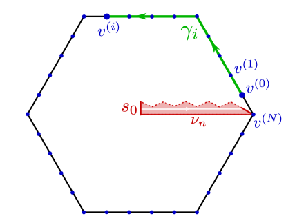
Figure 11: Vertices $v^{(i)}$ and direct paths $\sigma_{i}$ on the boundary of the region ${\Gamma}^{E}_{n}$, defined relative to the fiducial ribbon ${\nu_{n}}$. The region ${\Gamma}^{E}_{n}$ is indicated by the black hexagon. The individual edges of ${\Gamma}^{E}_{n}$ are not shown.

Before proving the Lemma on the free and transitive action of the gauge group $\mathcal{G}_{n}$, we show the following result, which will help us prove uniqueness statements for gauge transformations.

Lemma B.7.

If $\alpha\in\mathfrak{G}_{n}$ is any gauge configuration on ${\Gamma}^{E}_{n}$ and $U\in\mathcal{G}_{n}$ is such that $U\ket{\alpha}=\ket{\alpha}$, then $U=\mathds{1}$.

Proof.

Since $U\in\mathcal{G}_{n}$ it is of the form $U=\prod_{v\in{\Gamma}^{V}_{n}}\,A_{v}^{g_{v}}$ for group elements $g_{v}\in G$. For any edge $e=(v,v^{\prime})$ with $v\in\partial{\Gamma}^{V}_{n}$ and $v^{\prime}\in{\Gamma}^{V}_{n}$ we have $\alpha_{e}=\alpha_{e}\bar{g}_{v^{\prime}}$, so $g_{v}^{\prime}=1$. This shows that in fact $U\in\mathcal{G}_{n-1}$. Proceeding inductively, we find that $U\in\mathcal{G}_{0}$, i.e. $U$ is of the form $U=A_{v_{0}}^{g_{v_{0}}}$. Finally, by considering any edge $e=(v_{0},v)$ we find that $\alpha_{e}=g_{v_{0}}\alpha_{e}$ so $g_{v_{0}}=1$ and $U=\mathds{1}$. ∎

Lemma B.8.

For any $\alpha,\alpha^{\prime}\in\mathcal{P}_{n}^{b}$, there is a unique $U\in\mathcal{G}_{n}$ such that $U\ket{\alpha}=\ket{\alpha^{\prime}}$. Moreover, for any $\alpha\in\mathcal{P}_{n}^{b}$ and any $U\in\mathcal{G}_{n}$ we have $U\ket{\alpha}=\ket{\alpha^{\prime}}$ with $\alpha^{\prime}\in\mathcal{P}_{n}^{b}$. i.e. the gauge group $\mathcal{G}_{n}$ acts freely and transitively on $\mathcal{P}_{n}^{b}$.

Proof.

Let us first prove the claim in the case of trivial boundary conditions $b=\emptyset$.

Take $\alpha\in\mathcal{P}_{n}^{\emptyset}$, we first construct a gauge transformation $U\in\mathcal{G}_{n}$ such that $U\ket{\alpha}=\ket{\emptyset}$ where $\emptyset\in\mathcal{P}_{n}^{\emptyset}$ is the empty string net.

Pick $v_{*}\in\partial{\Gamma}^{V}_{n}$ and for any $v\in{\Gamma}^{V}_{n}\cup\partial{\Gamma}^{V}_{n}$, let $\gamma_{v}$ be a direct path from $v_{*}$ to $v$ (Figure 12) and set

$$g_{v}=\phi_{\gamma_{v}}(\alpha).$$

Note that because $\alpha$ has trivial flux everywhere, $g_{v}$ does not depend on the choice of $\gamma_{v}$ (Lemma B.2). Note moreover that $g_{v}=1$ for all $v\in\partial{\Gamma}^{V}_{n}$ because the boundary condition of $\alpha$ is trivial.

Let

$$U=\prod_{v\in{\Gamma}^{V}_{n}}\,A_{v}^{g_{v}}\prod_{v\in\partial{\Gamma}^{V}_{n}}\,\tilde{A}_{v}^{g_{v}}.$$

Since $g_{v}=1$ for all $v\in\partial{\Gamma}^{V}_{n}$ actually $U=\prod_{v\in{\Gamma}^{V}_{n}}\,A_{v}^{g_{v}}$ so $U$ is an element of $\mathcal{G}_{n}$. Now, $U\ket{\alpha}=\ket{\alpha^{\prime}}$ for some $\alpha^{\prime}\in\mathcal{P}_{n}^{\emptyset}$. We show now that $\alpha^{\prime}=\emptyset$.

For any edge $e=(v,v^{\prime})\in{\Gamma}^{E}_{n}\cup\partial{\Gamma}^{E}_{n}$ we find

$$\alpha^{\prime}_{e}=g_{v}\,\alpha_{e}\,\bar{g}_{v^{\prime}}=\phi_{\gamma_{v}}(\alpha)\,\alpha_{e}\,\bar{\phi}_{\gamma_{v^{\prime}}}(\alpha)=\phi_{\gamma_{v}e}(\alpha)\,\bar{\phi}_{\gamma_{v^{\prime}}}(\alpha)=1,$$

where we note that $\gamma_{v}e$ is, like $\gamma_{v^{\prime}}$, a direct path form $v_{*}$ to $v^{\prime}$, and the flux of $\alpha$ through a direct path depends only on the endpoints, because $\alpha$ has flat gauge everywhere. We conclude that $\alpha^{\prime}=\emptyset$ as required.

Now take arbitrary $\alpha,\alpha^{\prime}\in\mathcal{P}_{n}^{\emptyset}$. We have just shown that there are gauge transformations $U,V\in\mathcal{G}_{n}$ such that $U\ket{\alpha}=\ket{\emptyset}$ and $V\ket{\alpha^{\prime}}=\ket{\emptyset}$. It follows that $V^{*}U\ket{\alpha}=\ket{\alpha^{\prime}}$. This shows the existence part of the claim in the case of a trivial boundary condition.

Consider now a general boundary condition $b$ and take $\alpha_{b},\alpha^{\prime}_{b}\in\mathcal{P}_{n}^{b}$. From Lemma B.6 we get a boundary gauge transformation $U_{\emptyset b}\in\partial\mathcal{G}_{n}$ such that $U_{\emptyset b}\ket{\alpha_{b}}=\ket{\alpha_{\emptyset}}$ and $U_{\emptyset b}\ket{\alpha^{\prime}_{b}}=\ket{\alpha^{\prime}_{\emptyset}}$ for string nets $\alpha_{\emptyset},\alpha^{\prime}_{\emptyset}\in\mathcal{P}_{n}^{\emptyset}$. Applying the result above, we get a gauge transformation $U\in\mathcal{G}_{n}$ such that $U\ket{\alpha_{\emptyset}}=\ket{\alpha^{\prime}_{\emptyset}}$. Now

$$U\ket{\alpha_{b}}=UU_{\emptyset b}^{*}\ket{\alpha_{\emptyset}}=U_{\emptyset b}^{*}\,U\ket{\alpha_{\emptyset}}=U_{\emptyset b}^{*}\,\ket{\alpha^{\prime}_{\emptyset}}=\ket{\alpha^{\prime}_{b}},$$

where we used that all gauge transformations commute with each other. This concludes the proof of the existence part of the claim.

As for uniqueness, take $\alpha_{1},\alpha_{2}\in\mathcal{P}_{n}^{b}$ and suppose that $U,U^{\prime}\in\mathcal{G}_{n}$ both satisfy $U\ket{\alpha_{1}}=U^{\prime}\ket{\alpha_{1}}=\ket{\alpha_{2}}$. Then $U^{\prime}U^{*}\ket{\alpha_{2}}=\ket{\alpha_{2}}$ and it follows from Lemma B.7 that $U^{\prime}=U$.

It remains to show that if $\alpha\in\mathcal{P}_{n}^{b}$ and $U\in\mathcal{G}_{n}$, then $U\ket{\alpha}=\ket{\alpha^{\prime}}$ with $\alpha^{\prime}\in\mathcal{P}_{n}^{b}$. This is easily seen by noting that since $U$ is supported on ${\Gamma}^{E}_{n}\setminus\partial{\Gamma}^{E}_{n}$, it cannot change the boundary condition. Since all gauge transformations preserve the zero flux constraints (because $[A_{v}^{h},B_{f}]=0$ for all vertices $v$ and faces $f$, cf. Eqs. (16) and (17)), we obtain the claim. ∎

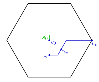
Figure 12: We pick a reference vertex $v_{*}$ and for any site, we pick an arbitrary direct path $\gamma_{v}$ from $v_{*}$ to $v$. Since $\alpha$ has trivial flux everywhere, $\phi_{\gamma_{v}}(\alpha)$ is independent of the path chosen.

Recall the boundary gauge transformations $\partial\mathcal{G}_{n}$ of Definition B.5.

Lemma B.9.

For any pair of boundary conditions $b,b^{\prime}\in\mathfrak{B}_{n}^{C}$ that are compatible with conjugacy class $C$ there is a boundary gauge transformation $U_{b^{\prime}b}\in\partial\mathcal{G}_{n}$ such that for any $\alpha\in\mathcal{P}_{n}^{C;ib}$ we have $U_{b^{\prime}b}\ket{\alpha}=\ket{\alpha^{\prime}}$ for an $\alpha^{\prime}\in\mathcal{P}_{n}^{C;ib^{\prime}}$ that satisfies $\alpha_{e}=\alpha^{\prime}_{e}$ for all $e\in{\Gamma}^{E}_{n-1}$.

Proof.

Fix a conjugacy class $C$ and a flux $c_{i}\in C$. We will first prove the claim for the simple boundary condition $b_{0}$ corresponding to the string net of Figure 13(a). i.e. let $b$ be an arbitrary boundary condition compatible with $C$. We will construct a boundary gauge transformation $U_{b_{0}b}\in\partial\mathcal{G}_{n}$ such that for any $\alpha\in\mathcal{P}_{n}^{C;ib}$ we have $U\ket{\alpha}=\ket{\alpha^{\prime}}$ with $\alpha^{\prime}\in\mathcal{P}_{n}^{C;ib_{0}}$ such that $\alpha_{e}=\alpha^{\prime}_{e}$ for all $e\in{\Gamma}^{E}_{n-1}.$

To that end, let $\partial{\Gamma}^{V}_{n}=\{v^{(0)},v^{(1)},\cdots,v^{(N)}\}$ be a labeling of the vertices in $\partial{\Gamma}^{V}_{n}$ as in Figure 11. For $i=1,\cdots,N$, let $\sigma_{i}$ be the direct path proceeding counterclockwise around $\partial{\Gamma}^{E}_{n}$ from $v^{(0)}$ to $v^{(i)}$ as in the Figure. Let $\sigma_{N+1}$ be the direct path that circles $\partial{\Gamma}^{E}_{n}$ in a counterclockwise direction starting and ending at $v^{(0)}$.

Since $\phi_{\sigma_{N+1}}(b)\in C$ it can be written as $\phi_{\sigma_{N+1}}(b)=c_{i^{\prime}}=qc_{i}\bar{q}$ for some $q\in G$. Set $g_{v^{(i)}}:=\bar{q}\,\phi_{\sigma_{i}}(b)$ and $U_{b_{0}b}=\prod_{i=1}^{N}\,\tilde{A}_{v^{(i)}}^{g_{v^{(i)}}}\in\partial\mathcal{G}_{n}$. Take $\alpha\in\mathcal{P}_{n}^{C;ib}$ and let $\alpha^{\prime}$ be the unique string net such that $U\ket{\alpha}=\ket{\alpha^{\prime}}$. Then for any $i=1,\cdots,N-1$ we set $e=(v^{(i)},v^{(i+1)})\in\partial{\Gamma}^{E}_{n}$, and find

$$b(\alpha^{\prime})_{e}=\alpha^{\prime}_{e}=g_{v^{(i)}}\,\alpha_{e}\,g_{v^{(i+1)}}=\bar{q}\phi_{\sigma_{i}}(b)b_{e}\bar{\phi}_{\sigma_{i+1}}(b)q=1.$$

Furthermore, for the final boundary edge $e=(v^{(N)},v^{(0)})$ we have

$$b(\alpha^{\prime})_{e}=\alpha^{\prime}_{e}=g_{v^{(N)}}\alpha_{e}\bar{g}_{v^{(0)}}=\bar{q}\phi_{\sigma_{N+1}}(b)q=c_{i}.$$

We conclude that $b(\alpha^{\prime})=b$. Moreover, since $U_{b_{0}b}$ is supported on ${\Gamma}^{E}_{n}\setminus{\Gamma}^{E}_{n-1}$ we have $\alpha_{e}=\alpha^{\prime}_{e}$ for all $e\in{\Gamma}^{E}_{n-1}$. This proves the existence part of the claim is this special case.

Using the same arguments one can show that if $\alpha\in\mathcal{P}_{n}^{C;ib_{0}}$, then $U_{b_{0}b}^{*}\ket{\alpha}=\ket{\alpha^{\prime}}$ for a string net $\alpha^{\prime}\in\mathcal{P}_{n}^{C;ib_{0}}$ such that $\alpha_{e}=\alpha^{\prime}_{e}$ for all $e\in{\Gamma}^{E}_{n-1}$.

Let us now prove the claim for general boundary conditions $b,b^{\prime}$ compatible with $C$.

We set $U_{b^{\prime}b}=U_{b_{0}b^{\prime}}^{*}U_{b_{0}b}\in\partial\mathcal{G}_{n}$ where the boundary gauge transformations $U_{b_{0}b}$ and $U_{b_{0}b^{\prime}}$ are as constructed above. then for any $\alpha\in\mathcal{P}_{n}^{C;ib}$ we have $U_{b^{\prime}b}\ket{\alpha}=\ket{\alpha^{\prime}}$ for a string net $\alpha^{\prime}\in\mathcal{P}_{n}^{C;ib^{\prime}}$ such that $\alpha_{e}=\alpha^{\prime}_{e}$ for all $e\in{\Gamma}^{E}_{n-1}$. This proves the general case. ∎

Recall the Definition 4.15 of the collections of string nets $\mathcal{P}_{n}^{C;ib}(m)$:

Fix a conjugacy class $C$, a boundary condition $b$ compatible with $C$ and a label $i=1,\cdots,|C|$. For any $m\in N_{C}$ we set

$$\mathcal{P}_{n}^{C;ib}(m):=\{\alpha\in\mathcal{P}_{n}^{C;ib}|\phi_{\nu_{n}}(\alpha)=q_{i}m\overline{q}_{i^{\prime}}\}$$

where $i^{\prime}=i(b)$.

Lemma B.10.

For any two $\alpha,\alpha^{\prime}\in\mathcal{P}_{n}^{C;ib}(m)$ there is a unique gauge transformation $U\in\overline{\mathcal{G}}_{n}$ such that $U\ket{\alpha}=\ket{\alpha^{\prime}}$. Moreover, if $\alpha\in\mathcal{P}_{n}^{C;ib}(m)$ and $U\in\overline{\mathcal{G}}_{n}$ then $U\ket{\alpha}=\ket{\alpha^{\prime}}$ with $\alpha^{\prime}\in\mathcal{P}_{n}^{C;ib}(m)$. i.e. $\overline{\mathcal{G}}_{n}$ acts freely and transitively on $\mathcal{P}_{n}^{C;ib}(m)$.

Proof.

Fix a conjugacy class $C$ and a flux $c_{i}\in C$. We will first prove the claim for the simple boundary condition $b_{0}$ corresponding to the string net of Figure 13(a). Denote by $\alpha^{(0)}\in\mathcal{P}_{n}^{C;ib_{0}}(1)$ the string net depicted in that figure. It has trivial gauge configuration everywhere except at the red edges. We will first show that for any $\alpha\in\mathcal{P}_{n}^{C;ib_{0}}$ there is a $U\in\overline{\mathcal{G}}_{n}$ such that $U\ket{\alpha}=\ket{\alpha^{(0)}}$.

Let $v_{*}\in\partial{\Gamma}^{V}_{n}$ be the vertex as defined in Figure 13(a). For any site $v\in{\Gamma}^{V}_{n}\cup\partial{\Gamma}^{V}_{n}$, let $\gamma_{v}$ be a direct path from $v_{*}$ to $v$ that does not contain any of the red edges (Lemma B.2). i.e. $\gamma_{v}$ is forbidden from crossing the fiducial ribbon. See Figure 13(a) for an example. Define $g_{v}:=\phi_{\gamma_{v}}(\alpha)$ for all $v\in{\Gamma}^{V}_{n}\cup\partial{\Gamma}^{V}_{n}$. Note that since $\alpha$ satisfies the flat gauge condition for all faces except for $f_{0}$, the group elements $g_{v}$ are independent of the choice of path $\gamma_{v}$, as long as we stick to paths that do not include red edges. (This strip acts a branch cut.) Note further that since the boundary condition is trivial everywhere except on the red boundary edge, we have $g_{v}=1$ for all $v\in\partial{\Gamma}^{V}_{n}$. Moreover, $g_{v_{0}}=1$ because we can take $\gamma_{v_{0}}$ to run along the direct part of the fiducial ribbon as in Figure 13(b). Since $\alpha\in\mathcal{P}_{n}^{C;ib_{0}}(1)$, we have $\phi_{{\nu_{n}}}(\alpha)=1$, therefore $g_{v_{0}}=1$.

Let

$$U=\prod_{v\in{\Gamma}^{V}_{n}}\,A_{v}^{g_{v}}\,\,\prod_{v\in\partial{\Gamma}^{V}_{n}}\,\tilde{A}_{v}^{g_{v}}=\prod_{v\in{\overline{\Gamma}}^{V}_{n}}\,A_{v}^{g_{b}}$$

where we used that $g_{v}=1$ for all $v\in\partial{\Gamma}^{V}_{n}$ and for $v=v_{0}$. i.e. we have $U\in\overline{\mathcal{G}}_{n}$.

We now let $\alpha^{\prime}\in\mathcal{P}_{n}^{C;ib_{0}}$ be the unique string net such that $U\ket{\alpha}=\ket{\alpha^{\prime}}$. We will show that $\alpha^{\prime}=\alpha^{(0)}$.

Let $e=(v,v^{\prime})$ be an edge that is not red. Then $\alpha^{\prime}_{e}=g_{v}\alpha_{e}\bar{g}_{v^{\prime}}=1$ because $g_{v}\alpha_{e}$ is the flux of $\alpha$ through $\gamma_{v}e$, which is a path from $v^{(N)}$ to $v^{\prime}$ that does not involve red edges. As noted before, that implies $g_{v}\alpha_{e}=g_{v^{\prime}}$. We see that $\alpha^{\prime}_{e}=1$ for all edges $e$ except possibly the red edges.

Let us now consider a red edge $e=(v,v^{\prime})$ which we take to be oriented upwards so that $\alpha^{(0)}_{e}=c_{i}$, see Figure 13(b). Let $I$ be the path from $v_{0}$ to $v$ and $II$ the path from $v_{0}$ to $v^{\prime}$ as shown in Figure 13(b). Then $\gamma_{v_{0}}I$ is a path from $v_{*}$ to $v$ and since $g_{v_{0}}=1$ we have $g_{v}=\phi_{I}(\alpha)$. Similarly, we have $g_{v^{\prime}}=\phi_{II}$. Let $\gamma_{s_{0}}$ be the direct path which starts and ends at $v_{0}$ and circles $f_{0}$ in a counterclockwise direction. The closed loop $Ie\overline{II}$ can be shrunk to $\gamma_{s_{0}}$ by a sequence of face-moves (Definition B.1) over faces $f\in{\overline{\Gamma}}^{F}_{n}$. Since $\alpha\in\mathcal{P}_{n}^{C;ib_{0}}$ we have $B_{f}\ket{\alpha}=\ket{\alpha}$ for all $f\in{\overline{\Gamma}}^{F}_{n}$ so it follows from Lemma B.2 that $c_{i}=\phi_{\gamma_{s_{0}}}(\alpha)=\phi_{Ie\overline{II}}(\alpha)=g_{v}\alpha_{e}\bar{g}_{v^{\prime}}=\alpha_{e}^{\prime}$.

Let now $\alpha_{1},\alpha_{2}\in\mathcal{P}_{n}^{C;ib_{0}}(1)$ be arbitrary. We have just shown that there are gauge transformations $U_{1},U_{2}\in\overline{\mathcal{G}}_{n}$ such that $U_{1}\ket{\alpha_{1}}=U_{2}\ket{\alpha_{2}}=\ket{\alpha^{(0)}}$. It follows that the gauge transformation $U=U_{2}^{*}U_{1}\in\overline{\mathcal{G}}_{n}$ satisfies $U\ket{\alpha}=\ket{\alpha^{\prime}}$. i.e. we have shown the existence claim in the special case of $\mathcal{P}_{n}^{C;ib_{0}}(1)$.

Let us now generalise to $\alpha_{1},\alpha_{2}\in\mathcal{P}_{n}^{C;ib_{0}}(m)$ for arbitrary $m\in N_{C}$. i.e. these string nets satisfy $\phi_{{\nu_{n}}}(\alpha_{1})=\phi_{{\nu_{n}}}(\alpha_{2})=q_{i}m\bar{q}_{i}$ where we noted that $i(b_{0})=i$.

Acting with the gauge transformation $U_{v_{0}}=A_{v_{0}}^{q_{i}\bar{m}\bar{q}_{i}}$ yields $U_{v_{0}}\ket{\alpha_{1}}=\ket{\alpha^{\prime}_{1}}$ and $U_{v_{0}}\ket{\alpha_{2}}=\ket{\alpha^{\prime}_{2}}$ for string nets $\alpha^{\prime}_{1},\alpha^{\prime}_{2}\in\mathcal{P}_{n}^{C;i}(1)$. Here the flux $c_{i}$ at $s_{0}$ was preserved because $q_{i}\bar{m}\bar{q}_{i}$ commutes with $c_{1}$, and the action of $A_{v_{0}}^{q_{i}\bar{m}\bar{q}_{i}}$ multiplies the flux through ${\nu_{n}}$ from the left by $q_{i}\bar{m}\bar{q}_{i}$, thus trivializing it.

Applying the above result, we have a gauge transformation $U\in\overline{\mathcal{G}}_{n}$ such that $U\ket{\alpha^{\prime}_{1}}=\ket{\alpha^{\prime}_{2}}$. Since $U$ commutes with $U^{*}_{v_{0}}$ we then find

$$U\ket{\alpha_{1}}=UU_{v_{0}}^{*}\ket{\alpha^{\prime}_{1}}=U_{v_{0}}^{*}\ket{\alpha^{\prime}_{2}}=\ket{\alpha_{2}}.$$

This proves the existence claim in the case of $\mathcal{P}_{n}^{C;ib_{0}}(m)$ for arbitrary $m\in N_{C}$.

Let us now consider a general boundary condition $b$ that is compatible with $C$. Take $\alpha_{1},\alpha_{2}\in\mathcal{P}_{n}^{C;ib}(m)\subset\mathcal{P}_{n}^{C;ib}$ for some $m\in N_{C}$. Lemma B.9 provides a boundary gauge transformation $U_{b_{0}b}\in\partial\mathcal{G}_{n}$ such that $U_{b_{0}b}\ket{\alpha_{1}}=\ket{\alpha^{\prime}_{1}}$ and $U_{b_{0}b}\ket{\alpha_{2}}=\ket{\alpha^{\prime}_{2}}$ for string nets $\alpha^{\prime}_{1},\alpha^{\prime}_{2}\in\mathcal{P}_{n}^{C;ib_{0}}(m^{\prime})$ for some $m^{\prime}\in N_{C}$. Here we noted that since $\alpha_{1}$ and $\alpha_{2}$ have the same flux through the fiducial ribbon ${\nu_{n}}$ and both are acted on by the same boundary gauge transformation $U_{b_{0}b}$, the resulting string nets $\alpha^{\prime}_{1}$ and $\alpha^{\prime}_{2}$ also have the same flux through ${\nu_{n}}$ (though possibly different from the fluxes of $\alpha_{1}$ and $\alpha_{2}$).

Using the result obtained above, we have a gauge transformation $U\in\overline{\mathcal{G}}_{n}$ such that $U\ket{\alpha^{\prime}_{1}}=\ket{\alpha^{\prime}_{2}}$. since $U$ commutes with $U_{b_{0}b}$ we find

$$U\ket{\alpha_{1}}=UU_{b_{0}b}^{*}\ket{\alpha^{\prime}_{1}}=U_{b_{0}b}^{*}U\ket{\alpha^{\prime}_{1}}=U_{b_{0}b}^{*}\ket{\alpha^{\prime}_{2}}=\ket{\alpha_{2}}.$$

This proves the existence part of the claim in full generality.

As for uniqueness, take $\alpha_{1},\alpha_{2}\in\mathcal{P}_{n}^{C;ib}(m)$ and suppose that $U,U^{\prime}\in\overline{\mathcal{G}}_{n}$ both satisfy $U\ket{\alpha_{1}}=U^{\prime}\ket{\alpha_{1}}=\ket{\alpha_{2}}$. Then $U^{\prime}U^{*}\ket{\alpha_{2}}=\ket{\alpha_{2}}$ and it follows from Lemma B.7 that $U^{\prime}=U$.

It remains to show that if $\alpha\in\mathcal{P}_{n}^{C;ib}(m)$ and $U\in\overline{\mathcal{G}}_{n}$, then $U\ket{\alpha}=\ket{\alpha^{\prime}}$ for an $\alpha^{\prime}\in\mathcal{P}_{n}^{C;ib}(m)$. To see this it is sufficient to note that $U$ is supported on ${\Gamma}^{E}_{n}\setminus\partial{\Gamma}^{E}_{n}$ and therefore it cannot change the boundary condition. Further, By Lemma A.13 any gauge transformation not supported on $v_{0}$ commutes with the projectors $B_{{s_{0}}}^{c_{i}}$, so $U\in\overline{\mathcal{G}}_{n}$ cannot change the label $i$. Finally, if $v\in{\overline{\Gamma}}^{V}_{n}$ then either no edges incident on $v$ belong to the direct path of the fiducial ribbon, in which case $\phi_{{\nu_{n}}}(\alpha^{\prime})=\phi_{{\nu_{n}}}(\alpha)$ is obvious. Or, precisely two edges incident on $v$ are part of the fiducial ribbon, say $e_{i}$ and $e_{i+1}$ where we have labeled the direct edges of the fiducial ribbon $\{e_{1},\cdots,e_{n}\}$ along the orientation of ${\nu_{n}}$. In that case, if $\ket{\alpha^{\prime}}=A_{v}^{h}\ket{\alpha}$, then $\alpha^{\prime}_{e_{i}}=\alpha_{e_{i}}\bar{h}$ and $\alpha^{\prime}_{e_{i+1}}=h\alpha_{e_{i+1}}$, and $\alpha$ and $\alpha^{\prime}$ agree on all other edges. It follows that

$$\phi_{{\nu_{n}}}(\alpha^{\prime})=\prod_{j=1}^{n}\alpha^{\prime}_{e_{j}}=\prod_{j=1}^{i-1}\alpha_{e_{j}}\times\alpha_{e_{i}}\bar{h}\,h\,\alpha_{e_{i+1}}\times\prod_{j=i+2}^{n}\,\alpha_{e_{j}}=\phi_{{\nu_{n}}}(\alpha).$$

We see that no $A_{v}^{h}\in\overline{\mathcal{G}}_{n}$ changes the flux through the fiducial ribbon. Since $\overline{\mathcal{G}}_{n}$ is generated by these on-site gauge transformations, we get the required result. ∎

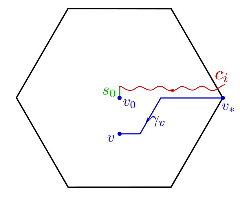
(a) A simple string net $\alpha^{(0)}\in\mathcal{P}_{n}^{C;i}$ that is non-trivial only on the dual part of the fiducial ribbon ${\nu_{n}}$. The corresponding boundary condition $b_{0}$ is trivial everywhere except at one edge.

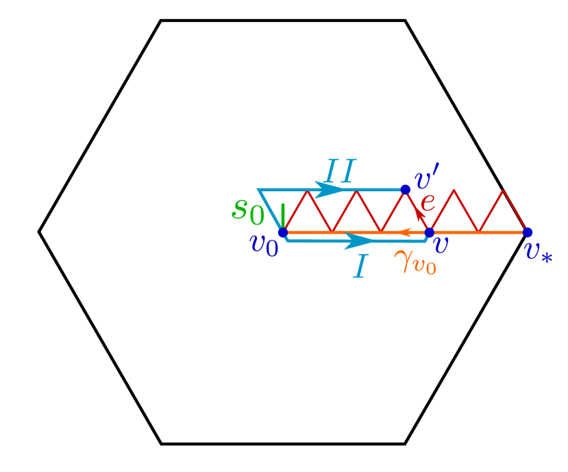
(b) Paths used in the proof of Lemma B.10.

Figure 13:

B.4 Action of ribbon operators on string-net states

Lemma B.11.

Suppose $\rho$ is a finite ribbon supported within $S\subset\Gamma^{E}$ and $\alpha\in\mathfrak{G}_{S}$. Then

$$T_{\rho}^{g}\ket{\alpha}=\delta_{\phi_{\rho}(\alpha),g}\ket{\alpha}$$

for any $g\in G$. In particular, $[T_{\rho}^{g},T_{\rho^{\prime}}^{g^{\prime}}]=0$ for all ribbons $\rho,\rho^{\prime}$ and any $g,g^{\prime}\in G$.

Proof.

We prove the Lemma by induction. If $\epsilon$ is the empty ribbon then $T_{\epsilon}^{g}=\delta_{1,g}\mathds{1}$, which says that the flux through the empty ribbon is always trivial. If $\rho=\{\tau\}$ consists of a single dual triangle then $T_{\rho}^{g}=F_{\rho}^{1,g}=\delta_{1,g}\mathds{1}$ which says that the flux through $\rho^{dir}=\emptyset$ is always trivial. If $\rho=\{\tau\}$ consists of a single direct triangle then $T_{\rho}^{g}=F_{\rho}^{1,g}=T_{\tau}^{g}$ which acts on the string net as $T_{\tau}^{g}\ket{\alpha}=\delta_{\alpha_{e_{\tau}},g}\ket{\alpha}=\delta_{\phi_{\tau}(\alpha),g}\ket{\alpha}$, as required.

Now suppose $\rho=\rho^{\prime}\tau$ and suppose the claim is true for the ribbon $\rho^{\prime}$. Then $T_{\rho}^{g}=\sum_{k}\,T_{\rho^{\prime}}^{k}T_{\tau}^{\bar{k}g}$. Using the above we get

$$T_{\rho}^{g}\,\ket{\alpha}=\sum_{k\in G}\delta_{\phi_{\rho^{\prime}}(\alpha),k}\delta_{\phi_{\tau}(\alpha),\bar{k}g}\ket{\alpha}=\delta_{\phi_{\rho}(\alpha),g}\ket{\alpha},$$

as required.

The commutativity can now be shown as follows. Let $S\subset\Gamma^{E}$ be finite and such that $S$ contains the supports of $T_{\rho}^{g}$ and $T_{\rho^{\prime}}^{g^{\prime}}$. Then for any $\alpha\in\mathfrak{G}_{S}$ we have

$$T_{\rho}^{g}T_{\rho^{\prime}}^{g^{\prime}}\ket{\alpha}=\delta_{\phi_{\rho}(\alpha),g}\delta_{\phi_{\rho^{\prime}}(\alpha),g^{\prime}}\ket{\alpha}=T_{\rho^{\prime}}^{g^{\prime}}T_{\rho}^{g}\ket{\alpha}.$$

Since $\ket{\alpha}$ for $\alpha\in\mathfrak{G}_{S}$ is an orthonormal basis for $\mathcal{H}_{S}$, the claim follows. ∎

Let us now consider the boundary ribbon $\beta_{n}$. Its alternating decomposition (Cf. Definition A.10) $\beta_{n}=I_{1}J_{1}\cdots I_{N}J_{N}$ has the direct parts $I_{i}=\{\tau_{i}\}$ consisting of a single triangle with $e_{\tau_{i}}\in\partial{\Gamma}^{E}_{n}$. The dual parts $J_{i}$ for $i=1,\cdots,N-1$ consist of one or two dual triangles each, corresponding to the edges of ${\Gamma}^{E}_{n}\setminus\partial{\Gamma}^{E}_{n}$ attached to each boundary vertex in $\partial{\Gamma}^{V}_{n}$. See Figure 14. For each boundary vertex $v$, let us write $J_{v}$ for the corresponding dual ribbon. Let us moreover order the boundary vertices $\partial{\Gamma}^{V}_{n}=\{v^{(1)},\cdots,v^{(N)}\}$ counterclockwise as in Figure 15.

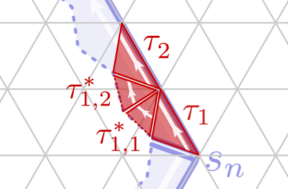
Figure 14: Examples of direct triangles $\tau_{i}$ and dual triangles $\tau^{*}_{i,1},\tau^{*}_{i,2}$ that make up the boundary ribbon $\beta_{n}$. The direct parts $I_{1}=\{\tau_{1}\}$ and $I_{2}=\{\tau_{2}\}$ as well as the first dual part $J_{1}=\{\tau^{*}_{1,1},\tau^{*}_{1,2}\}$ of $\beta_{n}$ are depicted.

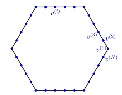
Figure 15: A clockwise labeling of the boundary vertices $\partial{\Gamma}^{V}_{n}$.

Let $\alpha\in\mathfrak{G}_{n}$ be a gauge configuration on ${\Gamma}^{E}_{n}$. With the notations just established, it follows from Lemma A.11 that

$$L_{\beta_{n}}^{h}\ket{\alpha}=\prod_{i=1}^{N}L_{J_{v^{(i)}}}^{\bar{K}_{i}hK_{i}}\ket{\alpha}$$ (24)

where

$$K_{i}=\prod_{j=1}^{i}\phi_{\tau_{i}}(\alpha)$$

is the flux of $\alpha$ through $\tau_{1}\cdots\tau_{i}$. Note that $K_{N}=\phi_{\beta_{n}}(b)$.

We can now prove

Lemma B.12.

Let $\alpha\in\mathcal{P}_{n}^{C;ib}$ and $h\in G$ that commutes with $\phi_{\beta_{n}}(b)$. Then $L_{\beta_{n}}^{h}\ket{\alpha}=\ket{\alpha^{\prime}}$ for a string net $\alpha^{\prime}\in\mathcal{P}_{n}^{C;ib}$ such that $\phi_{{\nu_{n}}}(\alpha^{\prime})=\phi_{{\nu_{n}}}(\alpha)h$.

Proof.

Using Eq. (24) one easily checks that for each face, except possibly the final one that contains the site $s_{n}$ (Figure 14), the action of $L_{\beta_{n}}^{h}$ preserves the trivial flux constraints.

For that final face, label its edges as in Figure 16. From Eq. (24) we see that the operator $L_{\beta_{n}}^{h}$ acts on the edge degrees of freedom of this triangle as $L_{e_{2}}^{\bar{K}_{1}\bar{h}K_{1}}R_{e_{3}}^{\bar{K}_{N}\bar{h}K_{N}}$. On the string net state $\alpha$ this becomes

$$L_{e_{2}}^{\bar{K}_{1}\bar{h}K_{1}}R_{e_{3}}^{\bar{K}_{N}\bar{h}K_{N}}\,\ket{\alpha_{e_{1}}}\otimes\ket{\alpha_{e_{2}}}\otimes\ket{\alpha_{e_{3}}}=\ket{\alpha_{e_{1}}}\otimes\ket{\bar{K}_{1}\bar{h}K_{1}\alpha_{e_{2}}}\otimes\ket{\alpha_{e_{3}}\bar{K}_{N}hK_{N}}.$$

Noting that $K_{N}=\phi_{\beta_{n}}(b)$ and $K_{1}=\alpha_{e_{1}}$ we see that the resulting flux measured at $s_{n}$ is

$$\bar{h}\alpha_{e_{1}}\alpha_{e_{2}}\alpha_{e_{3}}\overline{\phi_{\beta_{n}}(b)}\,h\phi_{\beta_{n}}(b)=\bar{h}\overline{\phi_{\beta_{n}}(b)}\,h\phi_{\beta_{n}}(b)$$

where we used that $\alpha$ satisfies the trivial flux constraint $\alpha_{e_{1}}\alpha_{e_{2}}\alpha_{e_{3}}=1$. We now use that $h$ commutes with the boundary flux $\phi_{\beta_{n}}(b)$ to see that the trivial flux condition is also maintained in the final face.

As already noted, $L_{\beta_{n}}^{h}$ acts on the degree of freedom at the edge $e_{3}$ as $R_{e_{3}}^{\bar{K}_{N}\bar{h}K_{N}}$, using again that $K_{N}=\phi_{\beta_{n}}(b)$ and $h$ commutes with $\phi_{\beta_{n}}(b)$ this is the same as $R_{e_{3}}^{\bar{h}}$. since $e_{2}$ is the final direct edge of the fiducial ribbon ${\nu_{n}}$, this immediately implies the final claim. ∎

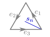
Figure 16: A labeling of the edges of the face $f(s_{n})$.

Recall from Definition 4.21 the unit vectors

$$\ket{\eta_{n}^{C;ib}(m)}=\frac{1}{\absolutevalue{\mathcal{P}_{n}^{C;ib}(m)}^{1/2}}\,\sum_{\alpha\in\mathcal{P}_{n}^{C;ib}(m)}\,\ket{\alpha}.$$

Lemma B.13.

For any $g\in G$, $C\in(G)_{cj},i=1,\cdots,\absolutevalue{C},b\in\mathfrak{B}_{n}^{C}$, and $m\in N_{C}$ we have

$$T_{\beta_{n}}^{g}\ket{\eta_{n}^{C;ib}(m)}=\delta_{g,q_{i(b)}r_{C}\,\bar{q}_{i(b)}}\ket{\eta_{n}^{C;ib}(m)}.$$

Proof.

By definition, $\ket{\eta_{n}^{C;ib(m)}}$ is a linear combination of states $\ket{\alpha}$ with $\alpha\in\mathcal{P}_{n}^{C;ib}(m)$ hence $\phi_{{\nu_{n}}}(\alpha)=q_{i}m\bar{q}_{i(b)}$ (cf. Definition 4.15) and $\phi_{f_{0}}(\alpha)=c_{i}$. It follows from Lemmas B.3 and B.4 that for all these string nets we have $\phi_{\beta_{n}}(\alpha)=\bar{\phi}_{{\nu_{n}}(\alpha)}c_{i}\phi_{{\nu_{n}}}(\alpha)=q_{i(b)}r_{C}\,\bar{q}_{i(b)}$. The result now follows immediately from Lemma B.11. ∎

Recall from Definition 4.26 the unit vectors

$$\ket{\eta_{n}^{RC;uv}}=\left(\frac{\mathrm{dim}R}{\absolutevalue{N_{C}}}\right)^{1/2}\,\sum_{m\in N_{C}}\,R^{jj^{\prime}}(m)\,\ket{\eta_{n}^{C;ib}(m)}$$

where $u=(i,j)\in I_{RC}$ and $v=(b,j^{\prime})\in I^{\prime}_{RC}$.

Lemma B.14.

We have

$$K_{\beta_{n}}^{R_{1}C_{1}}\ket{\eta_{n}^{R_{2}C_{2};uv}}=\delta_{R_{1}C_{1},R_{2}C_{2}}\,\ket{\eta_{n}^{R_{2}C_{2};uv}}.$$

Proof.

Let $u=(i,j)\in I_{R_{2}C_{2}}$ and $v=(b,j^{\prime})\in I^{\prime}_{R_{2}C_{2}}$, then

$$K_{\beta_{n}}^{R_{1}C_{1}}\,\ket{\eta_{n}^{R_{2}C_{2};uv}} =\sum_{\begin{subarray}{c}m_{1}\in N_{C_{1}}\\ m_{2}\in N_{C_{2}}\end{subarray}}\,\chi_{R_{1}}(m_{1})^{*}\,R_{2}^{jj^{\prime}}(m_{2})^{*}\,\sum_{q\in Q_{C_{1}}}\,L_{\beta_{n}}^{qm_{1}\bar{q}}\,T_{\beta_{n}}^{qr_{C_{1}}\bar{q}}\,\ket{\eta_{n}^{C_{2};ib}(m_{2})}$$

from Lemma B.13 and noting that $$qr_{C_{1}}\bar{q}=q_{i(b)}r_{C_{2}}\bar{q}_{i(b)} C_{1}=C_{2} q=q_{i(b)}$$ implies and we get

$$=\delta_{C_{1},C_{2}}\,\sum_{m_{1},m_{2}\in N_{C_{2}}}\,\chi_{R_{1}}(m_{1})^{*}\,R_{2}^{jj^{\prime}}(m_{2})^{*}\,L_{\beta_{n}}^{q_{b(i)}m_{1}\bar{q}_{i(b)}}\,\ket{\eta_{n}^{C_{2};ib}(m_{2})}$$

noting that $$\ket{\eta_{n}^{C_{2};ib}(m_{2})} \ket{\alpha} \alpha\in\mathcal{P}_{n}^{C;ib}(m_{2}) \alpha \phi_{\beta_{n}}=q_{i(b)}r_{C_{2}}\bar{q}_{i(b)}$$ is a linear combination of for , and for each such we have , it follows from Lemma B.12 that

$$=\delta_{C_{1},C_{2}}\,\sum_{m_{1},m_{2}\in N_{C_{2}}}\,\chi_{R_{1}}(m_{1})^{*}\,R_{2}^{jj^{\prime}}(m_{2})^{*}\,\ket{\eta_{n}^{C_{2};ib}(m_{2}m_{1})}$$

changing variables to $$M=m_{2}m_{1} m=m_{1}$$ and this becomes

$$=\delta_{C_{1},C_{2}}\,\sum_{M,m\in N_{C_{2}}}\,\chi_{R_{1}}(m)^{*}\,R_{2}^{jj^{\prime}}(M\bar{m})^{*}\,\ket{\eta_{n}^{C_{2};ib}(M)}$$

$$=\delta_{C_{1},C_{2}}\,\sum_{M,m\in N_{C_{2}}}\,\sum_{l,l^{\prime}}\,R_{1}^{ll}(m)^{*}\,R_{2}^{jl^{\prime}}(M)^{*}\,R_{2}^{j^{\prime}l^{\prime}}(m)\,\ket{\eta_{n}^{C_{2};ib}(M)}$$

Finally, applying Schur orthogonality we get

$$=\delta_{R_{1}C_{1},R_{2}C_{2}}\,\ket{\eta_{n}^{R_{2}C_{2};uv}},$$

finishing the proof. ∎

B.5 Action of Wigner projectors and label changers on string-net states

Recall the unit vectors (Definitions 4.21) and 4.26)

$$\ket{\eta_{n}^{C;ib}(m)}=\frac{1}{\absolutevalue{\mathcal{P}_{n}^{C;ib}(m)}^{1/2}}\,\sum_{\alpha\in\mathcal{P}_{n}^{C;ib}(m)}\,\ket{\alpha}$$

and

$$\ket{\eta_{n}^{RC;uv}}=\left(\frac{\mathrm{dim}R}{\absolutevalue{N_{C}}}\right)^{1/2}\,\sum_{m\in N_{C}}\,R^{jj^{\prime}}(m)^{*}\,\ket{\eta_{n}^{C;ib}(m)}$$

where $u=(i,j)\in I_{RC}$ and $v=(b,j^{\prime})\in I^{\prime}_{RC}$.

Recall from Definition 4.1 the Wigner projectors

$$D_{s}^{RC}:=\frac{\mathrm{dim}R}{|N_{C}|}\sum_{m\in N_{C}}\chi_{R}(m)^{*}\sum_{q\in Q_{C}}A_{s}^{qm\overline{q}}B_{s}^{qr_{C}\overline{q}}$$

and for each $u=(i,j)\in I_{RC}$

$$D_{s}^{RC;u}:=\frac{\mathrm{dim}R}{|N_{C}|}\sum_{m\in N_{C}}R^{jj}(m)^{*}A_{s}^{q_{i}m\overline{q}_{i}}B_{s}^{c_{i}}.$$

Lemma B.15.

We have

$$D_{{s_{0}}}^{R_{1}C_{1}}\ket{\eta_{n}^{R_{2}C_{2};uv}}=\delta_{R_{1}C_{1},R_{2}C_{2}}\ket{\eta_{n}^{R_{2}C_{2};uv}}.$$

Proof.

Let $u=(i,j)\in I_{RC}$ and $v=(b,j^{\prime})\in I^{\prime}_{RC}$. Then

$$D_{{s_{0}}}^{R_{1}C_{1}}\ket{\eta_{n}^{R_{2}C_{2};uv}} =\bigg{(}\frac{\dim R_{1}}{\absolutevalue{N_{C_{1}}}}\bigg{)}\bigg{(}\frac{\dim R_{2}}{\absolutevalue{N_{C_{2}}}}\bigg{)}^{1/2}\,\sum_{\begin{subarray}{c}m_{1}\in N_{C_{1}}\\ m_{2}\in N_{C_{2}}\end{subarray}}\,\chi_{R_{1}}(m_{1})^{*}R_{2}^{jj^{\prime}}(m_{2})^{*}\,$$

$$\quad\quad\quad\times\sum_{q\in Q_{C_{1}}}\,A_{{s_{0}}}^{qm_{1}\bar{q}}B_{{s_{0}}}^{qr_{C_{1}}\bar{q}}\,\ket{\eta_{n}^{C_{2};ib}(m_{2})}$$

$$=\delta_{C_{1},C_{2}}\,\frac{\dim R_{1}(\dim R_{2})^{1/2}}{\absolutevalue{N_{C_{1}}}^{3/2}}\,\sum_{m_{1},m_{2}\in N_{C_{1}}}\,\chi_{R_{1}}(m_{1})^{*}R_{2}^{jj^{\prime}}(m_{2})^{*}\,A_{{s_{0}}}^{q_{i}m_{1}\bar{q}_{i}}\,\ket{\eta_{n}^{C_{1};ib}(m_{2})}$$

using Lemma 4.23 this becomes

$$=\delta_{C_{1},C_{2}}\,\frac{\dim R_{1}(\dim R_{2})^{1/2}}{\absolutevalue{N_{C_{1}}}^{3/2}}\,\sum_{m_{1},m_{2}\in N_{C_{1}}}\,\chi_{R_{1}}(m_{1})^{*}R_{2}^{jj^{\prime}}(m_{2})^{*}\ket{\eta_{n}^{C_{1};ib}(m_{1}m_{2})}$$

changing variables to $$m=m_{1} M=m_{1}m_{2}$$ and we get

$$=\delta_{C_{1},C_{2}}\,\frac{\dim R_{1}(\dim R_{2})^{1/2}}{\absolutevalue{N_{C_{1}}}^{3/2}}\,\sum_{m,M\in N_{C_{1}}}\,\sum_{l,l^{\prime}}R_{1}^{ll}(m)^{*}R_{2}^{jl^{\prime}}(\bar{m})^{*}R_{2}^{l^{\prime}j^{\prime}}(M)^{*}\ket{\eta_{n}^{C_{1};ib}(M)}$$

using the Schur orthogonality relation (19)

$$=\delta_{R_{1}C_{1},R_{2}C_{2}}\,\bigg{(}\frac{\dim R_{1}}{\absolutevalue{N_{C_{1}}}}\bigg{)}^{1/2}\,\sum_{M\in N_{C_{1}}}\,R_{2}^{jj^{\prime}}(M)^{*}\ket{\eta_{n}^{C_{1};ib}(M)}$$

$$=\delta_{R_{1}C_{1},R_{2}C_{2}}\,\ket{\eta_{n}^{R_{1}C_{1};uv}}$$

as required. ∎

Lemma B.16.

We have

$$D_{{s_{0}}}^{RC;u_{1}}\,\ket{\eta_{n}^{RC;u_{2}v}}=\delta_{u_{1},u_{2}}\ket{\eta_{n}^{RC;u_{1}v}}.$$

Proof.

Let $u_{1}=(i_{1},j_{1})$, $u_{2}=(i_{2},j_{2})$ and $v=(b,j^{\prime})$. Then

$$D_{{s_{0}}}^{RC;u_{1}}\ket{\eta_{n}^{RC;u_{2}v}} =\bigg{(}\frac{\dim R}{\absolutevalue{N_{C}}}\bigg{)}^{3/2}\,\sum_{m_{1},m_{2}\in N_{C}}\,R^{j_{1}j_{1}}(m_{1})^{*}R^{j_{2}j^{\prime}}(m_{2})^{*}\,A_{{s_{0}}}^{q_{i_{1}}m_{1}\bar{q}_{i_{1}}}B_{{s_{0}}}^{c_{i_{1}}}\,\ket{\eta_{n}^{C;i_{2}b}(m_{2})}$$

noting that $$B_{{s_{0}}}^{c_{i_{1}}}\,\ket{\eta_{n}^{C;i_{2}b}(m_{2})}=\delta_{i_{1},i_{2}}$$ and using Lemma 4.23 this becomes

$$=\delta_{i_{1},i_{2}}\,\bigg{(}\frac{\dim R}{\absolutevalue{N_{C}}}\bigg{)}^{3/2}\,\sum_{m_{1},m_{2}\in N_{C}}\,R^{j_{1}j_{1}}(m_{1})^{*}R^{j_{2}j^{\prime}}(m_{2})^{*}\,\ket{\eta_{n}^{C;i_{2}b}(m_{1}m_{2})}$$

changing variables to $$m=m_{1} M=m_{1}m_{2}$$ and we get

$$=\delta_{i_{1},i_{2}}\,\bigg{(}\frac{\dim R}{\absolutevalue{N_{C}}}\bigg{)}^{3/2}\,\sum_{m,M\in N_{C}}\sum_{l^{\prime}}\,R^{j_{1}j_{1}}(m)^{*}R^{j_{2}l^{\prime}}(\bar{m})^{*}R^{l^{\prime}j^{\prime}}(M)^{*}\,\ket{\eta_{n}^{C;i_{2}b}(M)}$$

it then follows from the Schur orthogonality relation (19) that

$$=\delta_{u_{1},u_{2}}\,\bigg{(}\frac{\dim R}{\absolutevalue{N_{C}}}\bigg{)}^{1/2}\,\sum_{M\in N_{C}}R^{j_{2}j^{\prime}}(M)^{*}\,\ket{\eta_{n}^{C;i_{2}b}(M)}$$

$$=\delta_{u_{1},u_{2}}\,\ket{\eta_{n}^{RC;u_{2}v}}$$

as required. ∎

Recall the operators from Definition 4.30:

$$a_{s}^{RC;u_{2}u_{1}}:=\frac{\mathrm{dim}R}{|N_{C}|}\sum_{m\in N_{C}}R^{j_{2}j_{1}}(m)^{*}A_{s}^{q_{i_{2}}m\overline{q}_{i_{1}}}\qquad u_{1}=(i_{1},j_{1})\quad u_{2}=(i_{2},j_{2})$$

and

$$\tilde{a}_{n}^{RC;v_{2}v_{1}}:=\frac{\mathrm{dim}R}{|N_{C}|}\sum_{m\in N_{C}}R^{j^{\prime}_{2}j^{\prime}_{1}}(m)U_{b_{2}b_{1}}L_{\beta_{n}}^{{q_{i(b_{1})}\overline{m}\,\overline{q}_{i(b_{1})}}}\qquad v_{1}=(b_{1},j^{\prime}_{1})\quad u_{2}=(b_{2},j^{\prime}_{2})$$

where $U_{b_{2}b_{1}}$ is a unitary provided by Lemma B.9, which we choose such that $U_{b_{2}b_{1}}=(U_{b_{1}b_{2}})^{*}$. It follows from Lemma B.9 that the unitary $U_{b_{2}b_{1}}$ yields a bijection between $\mathcal{P}_{n}^{C;ib_{1}}$ and $\mathcal{P}_{n}^{C;ib_{2}}$ whenever $b_{1},b_{2}\in\mathfrak{B}_{n}^{C}$.

It was shown in Lemma 4.23 that the gauge transformations $A_{{s_{0}}}^{q_{i}m\bar{q}_{i}}$ for $m\in N_{C}$ yield a left group action of $N_{C}$ on the vectors $\ket{\eta_{n}^{C;ib}(m)}$. We show now that the operators $L_{\beta_{n}}^{q_{i(b)}\bar{m}\bar{q}_{i(b)}}$ for $m\in N_{C}$ yield a right action of $N_{C}$ on these vectors.

Lemma B.17.

For any $m_{1},m_{2}\in N_{C}$ we have

$$L_{\beta_{n}}^{q_{i(b)}\bar{m}_{1}\bar{q}_{i(b)}}\,\ket{\eta_{n}^{C;ib}(m_{2})}=\ket{\eta_{n}^{C;ib}(m_{2}\bar{m}_{1})}.$$

Proof.

From Lemma B.12 and the fact that $L_{\beta_{n}}^{q_{i(b)}\bar{m}_{1}\bar{q}_{i(b)}}$ is unitary, we see that this operator yields a bijection from $\mathcal{P}_{n}^{C;ib}(m_{2})$ to $\mathcal{P}_{n}^{C;ib}(m_{2}\bar{m}_{1})$. It follows that

$$L_{\beta_{n}}^{q_{i(b)}\bar{m}_{1}\bar{q}_{i(b)}}\,\ket{\eta_{n}^{C;ib}(m_{2})} =\frac{1}{\absolutevalue{\mathcal{P}_{n}^{C;ib}(m_{2})}^{1/2}}\,\sum_{\alpha\in\mathcal{P}_{n}^{C;ib}(m_{2})}\,L_{\beta_{n}}^{q_{i(b)}\bar{m}_{1}\bar{q}_{i(b)}}\,\ket{\alpha}$$

$$=\frac{1}{\absolutevalue{\mathcal{P}_{n}^{C;ib}(m_{2}\bar{m}_{1})}^{1/2}}\,\sum_{\alpha\in\mathcal{P}_{n}^{C;ib}(m_{2}\bar{m}_{1})}\,\ket{\alpha}$$

$$=\ket{\eta_{n}^{C;ib}(m_{2}\bar{m}_{1})}.$$

∎

We can now show

Lemma B.18.

For any $u,u_{1},u_{2}\in I_{RC}$ and any $v,v_{1},v_{2}\in I^{\prime}_{RC}$ we have

$$a_{{s_{0}}}^{RC;u_{2}u_{1}}\ket{\eta_{n}^{RC;u_{1}v}}=\ket{\eta_{n}^{RC;u_{2}v}},\quad\quad\tilde{a}_{n}^{RC;v_{2}v_{1}}\ket{\eta_{n}^{RC;uv_{1}}}=\ket{\eta_{n}^{RC;u,v_{2}}}$$

as well as

$$(a_{{s_{0}}}^{RC;u_{1}u_{2}})^{*}\ket{\eta_{n}^{RC;u_{1}v}}=\ket{\eta_{n}^{RC;u_{2}v}},\quad\quad(\tilde{a}_{n}^{RC;v_{1}v_{2}})^{*}\ket{\eta_{n}^{RC;uv_{1}}}=\ket{\eta_{n}^{RC;u,v_{2}}}.$$

Proof.

We prove the claim about the action of $\tilde{a}_{n}^{RC;v_{2}v_{1}}$. The claim about $(\tilde{a}_{n}^{RC;v_{1}v_{2}})^{*}$ is proven in exactly the same way, and the claims about $a_{{s_{0}}}^{RC;u_{2}u_{1}}$ and its hermitian conjugate have similar but simpler proofs. Let $u=(i,j)$, $v_{1}=(b_{1},j^{\prime}_{1})$ and $v_{2}=(b_{2},j^{\prime}_{2})$, then

$$\tilde{a}_{n}^{RC;v_{2}v_{1}}\ket{\eta_{n}^{RC;uv_{1}}} =\left(\frac{\mathrm{dim}R}{\absolutevalue{N_{C}}}\right)^{3/2}\,\sum_{m_{1},m_{2}\in N_{C}}\,R^{j^{\prime}_{2}j^{\prime}_{1}}(m_{2})\,R^{jj^{\prime}_{1}}(m_{1})^{*}\,U_{b_{2}b_{1}}\,L_{\beta_{n}}^{q_{i(b_{1})}\bar{m}_{2}\bar{q}_{i(b_{1})}}\,\ket{\eta_{n}^{C;ib_{1}}(m_{1})}$$

using Lemma B.17 and the basic properties of $$U_{b_{2}b_{1}}$$

$$=\left(\frac{\mathrm{dim}R}{\absolutevalue{N_{C}}}\right)^{3/2}\,\sum_{m_{1},m_{2}\in N_{C}}\,R^{j^{\prime}_{2}j^{\prime}_{1}}(m_{2})\,R^{jj^{\prime}_{1}}(m_{1})^{*}\,\ket{\eta_{n}^{C;ib_{2}}(m_{1}\bar{m}_{2})}$$

letting $$M=m_{1}\bar{m}_{2} m=m_{2}$$ and this becomes

$$=\left(\frac{\mathrm{dim}R}{\absolutevalue{N_{C}}}\right)^{3/2}\,\sum_{m,M\in N_{C}}\,R^{j^{\prime}_{2}j^{\prime}_{1}}(m)\,R^{jj^{\prime}_{1}}(Mm)^{*}\,\ket{\eta_{n}^{C;ib_{2}}(M)}$$

$$=\left(\frac{\mathrm{dim}R}{\absolutevalue{N_{C}}}\right)^{3/2}\,\sum_{m,M\in N_{C}}\sum_{l}\,R^{j^{\prime}_{2}j^{\prime}_{1}}(m)\,R^{jl}(M)^{*}\,R^{lj^{\prime}_{1}}(m)^{*}\,\ket{\eta_{n}^{C;ib_{2}}(M)}$$

using the Schur orthogonality relations

$$=\left(\frac{\mathrm{dim}R}{\absolutevalue{N_{C}}}\right)^{1/2}\,\sum_{M\in N_{C}}\,R^{jj^{\prime}_{2}}(M)^{*}\,\ket{\eta_{n}^{C;ib_{2}}(M)}$$

$$=\ket{\eta_{n}^{RC;uv_{2}}}.$$

∎

This Lemma tells us that $u$ is a “bulk” label, as the operator that changes $u_{1}$ to $u_{2}$ is $a_{{s_{0}}}^{RC;u_{2}u_{1}}\in\mathfrak{A}_{{\Gamma}^{E}_{1}}$. We also see that $v$ is a “boundary” label, as the operator that changes $v_{1}$ to $v_{2}$ is $\tilde{a}_{n}^{RC;v_{2}v_{1}}\in\mathfrak{A}_{{\Gamma}^{E}_{n}\setminus{\Gamma}^{E}_{n-1}}$.

We can also detect the boundary data by operators supported on ${\Gamma}^{E}_{n}\setminus{\Gamma}^{E}_{n-1}$. Recall from Definition 3.2 the projectors $P_{b}$ supported on $\partial{\Gamma}^{E}_{n}$ that project onto states with boundary condition $b\in\mathfrak{B}_{n}$.

Lemma B.19.

For any $u\in I_{RC}$, and any $v_{1},v_{2}\in I^{\prime}_{RC}$ we have

$$\tilde{a}_{n}^{RC;v_{2}v_{2}}P_{b_{2}}\ket{\eta_{n}^{RC;uv_{1}}}=\delta_{v_{1},v_{2}}\,\ket{\eta_{n}^{RC;uv_{1}}}.$$

Proof.

Let $u=(i,j)$, $v_{1}=(b_{1},j^{\prime}_{1})$, and $v_{2}=(b_{2},j^{\prime}_{2})$. Then

$$\tilde{a}_{n}^{RC;v_{2}v_{2}}P_{b_{2}}\ket{\eta_{n}^{RC;uv_{1}}} =\left(\frac{\mathrm{dim}R}{\absolutevalue{N_{C}}}\right)^{3/2}\,\sum_{m_{1},m_{2}\in N_{C}}\,R^{j^{\prime}_{2}j^{\prime}_{2}}(m_{2})\,R^{jj^{\prime}_{1}}(m_{1})^{*}\,U_{b_{2}b_{2}}\,L_{\beta_{n}}^{q_{i(b_{1})}\bar{m}_{2}\bar{q}_{i(b_{1})}}\,P_{b_{2}}\ket{\eta_{n}^{C;ib_{1}}(m_{1})}$$

using Lemma B.17 and the basic properties of $$U_{b_{2}b_{1}} P_{b_{2}}$$ and we get

$$=\delta_{b_{1},b_{2}}\,\left(\frac{\mathrm{dim}R}{\absolutevalue{N_{C}}}\right)^{3/2}\,\sum_{m_{1},m_{2}\in N_{C}}\,R^{j^{\prime}_{2}j^{\prime}_{2}}(m_{2})\,R^{jj^{\prime}_{1}}(m_{1})^{*}\,\ket{\eta_{n}^{C;ib_{2}}(m_{1}\bar{m}_{2})}$$

letting $$M=m_{1}\bar{m}_{2} m=m_{2}$$ and this becomes

$$=\delta_{b_{1},b_{2}}\left(\frac{\mathrm{dim}R}{\absolutevalue{N_{C}}}\right)^{3/2}\,\sum_{m,M\in N_{C}}\,R^{j^{\prime}_{2}j^{\prime}_{2}}(m)\,R^{jj^{\prime}_{1}}(Mm)^{*}\,\ket{\eta_{n}^{C;ib_{2}}(M)}$$

$$=\delta_{b_{1},b_{2}}\left(\frac{\mathrm{dim}R}{\absolutevalue{N_{C}}}\right)^{3/2}\,\sum_{m,M\in N_{C}}\sum_{l}\,R^{j^{\prime}_{2}j^{\prime}_{2}}(m)\,R^{jl}(M)^{*}\,R^{lj^{\prime}_{1}}(m)^{*}\,\ket{\eta_{n}^{C;ib_{2}}(M)}$$

using the Schur orthogonality relations

$$=\delta_{b_{1},b_{2}}\delta_{j^{\prime}_{1},j^{\prime}_{2}}\,\left(\frac{\mathrm{dim}R}{\absolutevalue{N_{C}}}\right)^{1/2}\,\sum_{M\in N_{C}}\,R^{jj^{\prime}_{2}}(M)^{*}\,\ket{\eta_{n}^{C;ib_{2}}(M)}$$

$$=\delta_{v_{1},v_{2}}\,\ket{\eta_{n}^{RC;uv_{2}}}.$$

∎

Appendix C Properties of cone algebras

In this appendix we prove some properties of cone algebras used in Section 5. These results are slight extensions and elaborations of result previously obtained in [Naa11, Naa15] and [Key+06]. See also [Oga23].

Let $\Lambda$ be a cone and write $\mathcal{R}(\Lambda)=\pi_{0}(\mathfrak{A}_{\Lambda})^{\prime\prime}$ for the von Neumann algebra generated by $\pi_{0}(\mathfrak{A}_{\Lambda})$. The following is an adaptation of Theorem 5.2 of [Naa11], which is itself and adaptation of Proposition 5.3 of [Key+06].

Proposition C.1.

The von Neumann algebra $\mathcal{R}(\Lambda)$ is an infinite factor.

Proof.

To see that $\mathcal{R}(\Lambda)$ is a factor, let $\mathcal{Z}=\mathcal{R}(\Lambda)\cap\mathcal{R}(\Lambda)^{\prime}$ be its center. Then $\mathcal{Z}^{\prime}=\mathcal{R}(\Lambda)\vee\mathcal{R}(\Lambda)^{\prime}$. Since $\mathcal{R}(\Lambda^{c})\subset\mathcal{R}(\Lambda)^{\prime}$, we have:

$$\mathcal{R}(\Lambda)\vee\mathcal{R}(\Lambda^{c})\subset\mathcal{Z}^{\prime}$$

But $\mathcal{R}(\Lambda)\vee\mathcal{R}(\Lambda^{c})=\mathcal{B}(\mathcal{H}_{0})$, so we find $\mathcal{Z}^{\prime}=\mathcal{B}(\mathcal{H}_{0})$ and therefore $\mathcal{Z}=\mathbb{C}\mathds{1}$. This shows that $\mathcal{R}(\Lambda)$ is a factor.

To see that $\mathcal{R}(\Lambda)$ is an infinite factor, we argue by contradiction. Suppose $\mathcal{R}(\Lambda)$ were a finite factor. Then there is a unique faithful normal trace $\tau$ on $\mathcal{R}(\Lambda)$ which induces a tracial state $\tilde{\tau}:=\tau\circ\pi_{0}$ on $\mathfrak{A}_{\Lambda}$. Since $\mathfrak{A}_{\Lambda}$ is a UHF algebra, this tracial state is unique and satisfies $\tilde{\tau}(OO^{\prime})=\tilde{\tau}(O)\tilde{\tau}(O^{\prime})$ for all $O,O^{\prime}\in\mathfrak{A}$ with disjoint supports. It follows from this and Theorem 2.6.10 of [BR12] that $\tilde{\tau}$ is a factor state.

Recall that $\pi_{0}:\mathfrak{A}\rightarrow\mathcal{B}(\mathcal{H}_{0})$ is the GNS representation of the pure frustration free ground state $\omega_{0}$, and the frustration free ground state corresponds in this representation to the unit vector $|\Omega_{0}\rangle\in\mathcal{H}_{0}$. This vector also corresponds to the restricted state $\omega_{0}|_{\mathfrak{A}_{\Lambda}}$ in the restricted representation $\pi_{0}|_{\mathfrak{A}_{\Lambda}}$ (although it is not the only vector in $\mathcal{H}_{0}$ with this property). This shows in particular that $\omega_{0}|_{\mathfrak{A}_{\Lambda}}$ is $\pi_{0}|_{\mathfrak{A}_{\Lambda}}$-normal. Since $\mathcal{R}(\Lambda)$ is a factor, $\pi_{0}|_{\mathfrak{A}_{\Lambda}}$ is a factor representation of $\mathfrak{A}_{\Lambda}$. It then follows from Proposition 10.3.14 of [KR86] that the GNS representation of $\omega_{0}|_{\mathfrak{A}_{\Lambda}}$ is quasi-equivalent to $\pi_{0}|_{\mathfrak{A}_{\Lambda}}$, and therefore the states $\omega_{0}|_{\mathfrak{A}_{\Lambda}}$ and $\tilde{\tau}$ are quasi-equivalent.

From Corollary 2.6.11 of [BR12] we have for each $\epsilon>0$ a finite set $\Gamma_{\epsilon}\subset\Lambda$ such that $\absolutevalue{\omega_{0}(O)-\tilde{\tau}(O)}<\epsilon\norm{O}$ for all $O\in\mathfrak{A}_{\Lambda\setminus\Gamma_{\epsilon}}$. If $O,O^{\prime}\in\mathfrak{A}_{\Lambda\setminus\Gamma_{\epsilon}}$ then, using that $\tilde{\tau}$ is a trace, we find

$$\absolutevalue{\omega_{0}(OO^{\prime})-\omega_{0}(O^{\prime}O)} =\absolutevalue{\omega_{0}(OO^{\prime})-\tilde{\tau}(OO^{\prime})+\tilde{\tau}(O^{\prime}O)-\omega_{0}(O^{\prime}O)}$$

$$=\absolutevalue{\omega_{0}(OO^{\prime})-\tilde{\tau}(OO^{\prime})}+\absolutevalue{\omega_{0}(O^{\prime}O)-\tilde{\tau}(O^{\prime}O)}$$

$$<\epsilon\,(\norm{OO^{\prime}}+\norm{O^{\prime}O}),$$ (25)

i.e. the frustration free ground state is approximately tracial at infinity. One could use translation invariance to conclude that $\omega_{0}$ actually is a tracial state, leading to contradiction. Here we simply provide a counterexample as follows.

Let $\rho$ be a finite ribbon supported in $\Lambda\setminus\Gamma_{\epsilon}$ with initial site $s_{0}=\partial_{0}\rho$, and choose any non-trivial $RC$ and label $u$. Then it follows from Lemmas A.26 and A.19 that

$$\omega_{0}\big{(}\sum_{v}(F_{\rho}^{RC;uv})^{*}\,D_{s_{0}}^{RC;u}\,F_{\rho}^{RC;uv}\big{)}=1.$$ (26)

On the other hand, from Eq. (25) we get

$$\absolutevalue{\omega_{0}\big{(}\sum_{v}(F_{\rho}^{RC;uv})^{*}\,D_{s_{0}}^{RC;u}\,F_{\rho}^{RC;uv}\big{)}-\omega_{0}\big{(}\sum_{v}F_{\rho}^{RC;uv}\,(F_{\rho}^{RC;uv})^{*}D_{s_{0}}^{RC;u}\big{)}}<\epsilon C$$

for some $C$ that only depends on the norms of the operators involved. In particular, $C$ does not depend on $\epsilon$. But for any local operator $O$, we have from Lemma A.25 that

$$\omega_{0}\big{(}OD_{s_{0}}^{RC;u}\big{)}=0$$

So we find

$$\absolutevalue{\omega_{0}\big{(}\sum_{v}(F_{\rho}^{RC;uv})^{*}\,D_{s_{0}}^{RC;u}\,F_{\rho}^{RC;uv}\big{)}}<\epsilon C.$$

Taking $\epsilon$ small enough, this contradicts Eq. (26).

We conclude that $\mathcal{R}(\Lambda)$ is an infinite factor as required. ∎

Elaborating on Corollary 5.3 of [Naa11], we get the following result:

Corollary C.2.

For any $n\in\mathbb{N}$ we can find isometries $\{V_{i}\}_{i=1}^{n}$ in $\mathcal{R}(\Lambda)$ such that $\sum_{i}V_{i}V_{i}^{*}=\mathds{1}$ and $V_{i}^{*}V_{j}=\delta_{i,j}\mathds{1}$.

Proof.

By Proposition C.1 the von Neumann algebra $\mathcal{R}(\Lambda)$ is an infinite factor. In particular, all its infinite projectors are properly infinite.

For any infinite (and therefore properly infinite) projector $P\in\mathcal{R}(\Lambda)$, the Halving lemma (Lemma 6.3.3 of [KR86]) gives a projector $Q\in\mathcal{R}(\Lambda)$ such that $Q\leq P$ and $Q\sim(P-Q)\sim P$ (Here $\sim$ denotes Murray-von Neumann equivalence of projectors). Moreover, $Q$ and $P-Q$ are orthogonal to each other and they are both infinite. To see this, assume one of them is finite. Then they are both finite by equivalence and therefore $Q+(P-Q)=P$ is finite, which contradicts the assumption.

Applying this repeatedly to the identity, we get $n$ orthogonal projectors $P_{1},\cdots,P_{n}$ such that $\sum_{i}P_{i}=\mathds{1}$ and $P_{i}\sim\mathds{1}$ for each $i=1,\cdots,n$. The equivalence $P_{i}\sim\mathds{1}$ means that there are isometries $\{V_{i}\}_{i=1}^{n}$ such that $P_{i}=V_{i}V_{i}^{*}$ and $V_{i}^{*}V_{i}=\mathds{1}$. It remains to show that $V_{i}^{*}V_{j}=\delta_{i,j}\mathds{1}$. Indeed we have $P_{i}P_{j}=\delta_{i,j}P_{i}$, hence $V_{i}V_{i}^{*}V_{j}V_{j}^{*}=\delta_{i,j}V_{i}V_{i}^{*}$. Multiplying to the left by $V_{i}^{*}$ and to the right by $V_{i}$ and using $V_{i}^{*}V_{i}=\mathds{1}$ then yields $V_{i}V_{j}^{*}=\delta_{i,j}\,\mathds{1}$ as required. ∎

Appendix D Projectors to enforce constraints in infinite regions

We consider a representation $\pi:\mathfrak{A}\rightarrow\mathcal{B}(\mathcal{H})$ of the quasi-local algebra, and use the notations of Section 6.1.

Let $S\subset{\Gamma^{VF}}$ be a finite region. Let $S^{V}:=S\cap\Gamma^{V}$ and $S^{F}:=S\cap\Gamma^{F}$. We define the projector $P_{S}\in\mathfrak{A}_{loc}$ by

$$P_{S}:=\prod_{v\in S^{V}}A_{v}\prod_{f\in S^{F}}B_{f}.$$

In this appendix, our aim is to define analogous projectors for infinite regions $S$.

Definition D.1.

An increasing sequence of sets $S_{n}\in{\Gamma^{VF}}$ is said to converge to $S\subset{\Gamma^{VF}}$ if $S_{n}\subset S$ for all $n\in\mathbb{N}$ and for each $x\in S$ there exists some $n_{0}$ such that $x\in S_{n}$ for all $n>n_{0}$.

Let $S_{n}$ be an increasing sequence of finite sets converging to a possibly infinite $S\in{\Gamma^{VF}}$.

The operators $\pi(P_{S_{n}})$ are projectors acting on the Hilbert space $\mathcal{H}$. Let us denote their ranges by $\mathcal{V}_{S_{n}}\subset\mathcal{H}$. The spaces $\mathcal{V}_{S_{n}}$ are closed subspaces of $\mathcal{H}$ and $\mathcal{V}_{S_{m}}\supset\mathcal{V}_{S_{n}}$ for all $m\leq n$. We define the space $\mathcal{V}_{S}\subset\mathcal{H}$ as follows

$$\mathcal{V}_{S}:=\bigcap_{n}\mathcal{V}_{S_{n}}=\{\ket{\psi}\in\mathcal{H}|\ket{\psi}\in\mathcal{V}_{S_{n}}\text{ for all }n\}\subset\mathcal{H}$$

Lemma D.2.

$\mathcal{V}_{S}$ is a closed linear subspace of $\mathcal{H}$.

Proof.

By definition, $\mathcal{V}_{S}\subset\mathcal{H}$. Suppose a sequence of vectors $\ket{\psi_{i}}\in\mathcal{V}_{S}$ converges in norm to $\ket{\psi}\in\mathcal{H}$. Then since $\mathcal{V}_{S}\subset\mathcal{V}_{S_{n}}$ for any $n$, the sequence $\ket{\psi_{i}}$ is contained in the closed space $\mathcal{V}_{S_{n}}$, and therefore the limit is as well. That is, $\ket{\psi}\in\mathcal{V}_{S_{n}}$ for all $n$. By definition, this means $\ket{\psi}\in\mathcal{V}_{S}$. This proves that $\mathcal{V}_{S}$ is closed. Linearity is shown in a similar way. ∎

Lemma D.3.

$\ket{\psi}\in\mathcal{V}_{S}$ if and only if $\pi(A_{v})\ket{\psi}=\pi({B_{f}})\ket{\psi}=\ket{\psi}$ for all $v\in S^{V}$ and $f\in S^{F}$.

Proof.

In order for $\ket{\psi}\in\mathcal{V}_{S}$ we must have $\ket{\psi}\in\mathcal{V}_{S_{n}}$ for all $n$, that is $\pi(P_{S_{n}})\ket{\psi}=\ket{\psi}$ for all $n$. If $v\in S^{V}$ then there exists some $n_{0}\in\mathbb{N}$ such that $v\in S_{n}$ for all $n\geq n_{0}$. Then we have for any $n\geq n_{0}$,

$$\pi(A_{v})\ket{\psi}=\pi(A_{v})\pi(P_{S_{n}})\ket{\psi}=\pi(A_{v}P_{S_{n}})\ket{\psi}=\pi(P_{S_{n}})\ket{\psi}=\ket{\psi}$$

where we have used the definition of $P_{S}$ and that $A_{v}$ is a projector to get $A_{v}P_{S_{n}}=P_{S_{n}}$. Similarly, if $f\in S^{F}$ then $\pi(B_{f})\ket{\psi}=\ket{\psi}$. This shows $(\implies)$.

To show $(\impliedby)$, let $\ket{\psi}$ be such that $\pi(A_{v})\ket{\psi}=\pi(B_{f})\ket{\psi}=\ket{\psi}$ for all $v\in S^{V}$ and all $f\in S^{F}$. Then using $S_{n}\subset S$ for all $n$, and $[A_{v},B_{f}]=0$ (Lemma A.1), we get

$$\pi(P_{S_{n}})\ket{\psi}=\pi\left(\prod_{v\in S^{V}_{n}}A_{v}\prod_{f\in S^{F}_{n}}B_{f}\right)\ket{\psi}=\prod_{v\in S_{n}^{V}}\pi(A_{v})\prod_{f\in S_{n}^{F}}\pi(B_{f})\ket{\psi}=\ket{\psi},$$

which shows $\ket{\psi}\in\mathcal{V}_{S_{n}}$ for all $n$. We conclude that $\ket{\psi}\in\mathcal{V}_{S}$. ∎

It follows that $\mathcal{V}_{S}$ depends only on $S$, not on the sequence $S_{n}\rightarrow S$ used in its construction.

Definition D.4.

For any $S\subset\Gamma^{VF}$ we let $p_{S}\in\mathcal{B}(\mathcal{H})$ be the projector onto the closed subspace $\mathcal{V}_{S}\subset\mathcal{H}$.

Lemma D.5.

If $S$ is finite, then $p_{S}=\pi(P_{S})$.

Proof.

For any $\ket{\psi}\in\mathcal{V}_{S}$ we have from Lemma D.3 that $\pi(A_{v})\ket{\psi}=\pi(B_{f})\ket{\psi}=\ket{\psi}$ for all $v\in S^{V},f\in S^{F}$. This implies

$$\pi\big{(}\prod_{v\in S^{V}}A_{v}\prod_{f\in S^{F}}B_{f}\big{)}\ket{\psi}=\pi(P_{S})\ket{\psi}=\ket{\psi}$$

so $\mathcal{V}_{S}\subseteq\text{Ran}(\pi(P_{S}))$.

Conversely, let $\pi(P_{S})\ket{\psi}=\ket{\psi}$. If $\langle{\psi},{\pi(A_{v}){\psi}}\rangle<1$ for any $v\in S^{V}$, then using $[A_{v},B_{f}]=0$ (Lemma A.1), we get $\langle{\psi},{\pi(P_{S})\psi}\rangle<1$, which is a contradiction. So for all $v\in S^{V}$, we must have $\langle{\psi},{\pi(A_{v})\psi}\rangle=1$. Since $A_{v}$ is a projector, we get $\pi(A_{v})\ket{\psi}=\ket{\psi}$ for all $v\in S^{V}$. From a similar argument for $B_{f}$, we get

$$\pi(A_{v})\ket{\psi}=\pi(B_{f})\ket{\psi}=\ket{\psi}$$

for all $v\in S^{V}$ and all $f\in S^{F}$. It follows from Lemma D.3 that $\ket{\psi}\in\mathcal{V}_{S}$, so $\text{Ran}(\pi(P_{S}))\subseteq\mathcal{V}_{S}$.

This shows that $\text{Ran}(\pi(P_{S}))=\mathcal{V}_{S}$ so $\pi(P_{S})=p_{S}$. ∎

Lemma D.6.

We have $p_{S}\ket{\psi}=\ket{\psi}$ if and only if $\pi(A_{v})\ket{\psi}=\pi(B_{f})\ket{\psi}=\ket{\psi}$ for all $v\in S^{V}$ and $f\in S^{F}$

Proof.

Follows immediately from Lemma D.3. ∎

The following Lemma is an immediate consequence of the standard fact that a bounded increasing sequence of non-negative operators converges in the strong operator topology.

Lemma D.7.

If $S_{n}$ is an increasing sequence of finite regions converging to S, then $p_{S}$ is the limit of $p_{S_{n}}$ in the strong operator topology.

Lemma D.8.

For any $X,Y\in\Gamma^{VF}$ we have

$$p_{X}p_{Y}=p_{X\cup Y}.$$

Proof.

First assume $X$ is finite. Since $p_{Y}$ is the strong limit of a sequence of projectors $p_{Y_{n}}$ for finite $Y_{n}$ (Lemma D.7) we have that $p_{X}p_{Y}$ is the strong limit of the sequence $p_{X}p_{Y_{n}}=p_{X\cup Y_{n}}$ (where the last equality uses that $X$ and $Y_{n}$ are finite). But the increasing sequence of finite sets $X\cup Y_{n}$ converges to $X\cup Y$ so by Lemma D.7 the strong limit is $p_{X\cup Y}$, proving the result in this case.

For general $X,Y$, note that there is an increasing sequence of finite sets $X_{n}$ converging to $X$ so that $p_{X_{n}}$ converges strongly to $p_{X}$. It follows that $p_{X_{n}}\,p_{Y}$ converges strongly to $p_{X}p_{Y}$. But we have just shown that $p_{X_{n}}\,p_{Y}=p_{X_{n}\cup Y}$, which by Lemma D.7 converges strongly to $p_{X\cup Y}$, proving the claim. ∎

References

- [DHR71] S. Doplicher, R. Haag and J.. Roberts “Local observables and particle statistics I” In Commun. Math. Phys. 23.3 Springer ScienceBusiness Media LLC, 1971, pp. 199–230
- [DHR74] S. Doplicher, R. Haag and J.. Roberts “Local observables and particle statistics II” In Commun. Math. Phys. 35, 1974, pp. 49–85
- [KR86] R.. Kadison and J.. Ringrose “Fundamentals of the theory of operator algebras. Volume II: Advanced theory” Academic press New York, 1986
- [FRS89] K. Fredenhagen, K.H. Rehren and B. Schroer “Superselection sectors with braid group statistics and exchange algebras: I. General theory” In Communications in Mathematical Physics 125 Springer, 1989, pp. 201–226
- [FG90] J. Fröhlich and F. Gabbiani “Braid statistics in local quantum theory” In Reviews in Mathematical Physics 2.03 World Scientific, 1990, pp. 251–353
- [FRS92] K. Fredenhagen, K.H. Rehren and B. Schroer “Superselection sectors with braid group statistics, II” In Rev. Math. Phys. SI1, 1992, pp. 113–157
- [Gou93] M.. Gould “Quantum double finite group algebras and their representations” In Bull. Aust. Math. Soc. 48.2 Cambridge University Press, 1993, pp. 275–301
- [SV93] K. Szlachányi and P. Vecsernyés “Quantum symmetry and braid group statistics in G-spin models” In Communications in mathematical physics 156 Springer, 1993, pp. 127–168
- [FGV94] J. Fuchs, A. Ganchev and P. Vecsernyés “The quantum symmetry of rational field theories” In Theoretical and Mathematical Physics 98.3 Springer, 1994, pp. 266–276 arXiv:hep-th/9407013
- [Vec94] P. Vecsernyés “On the quantum symmetry of the chiral Ising model” In Nuclear Physics B 415.3 Elsevier, 1994, pp. 557–588 arXiv:hep-th/9306118
- [NS97] F. Nill and K. Szlachányi “Quantum chains of Hopf algebras with quantum double cosymmetry” In Communications in mathematical physics 187.1 Springer, 1997, pp. 159–200 arXiv:hep-th/9509100
- [Fre98] M. Freedman “P/NP, and the quantum field computer” In Proc. Natl. Acad. Sci. U. S. A. 95.1, 1998, pp. 98–101
- [Kit03] A.. Kitaev “Fault-tolerant quantum computation by anyons” In Ann. Phys. 303.1, 2003, pp. 2–30 arXiv:quant-ph/9707021
- [LW04] M. Levin and X.-G. Wen “String-net condensation: A physical mechanism for topological phases”, 2004 arXiv:cond-mat/0404617
- [Key+06] M. Keyl, T. Matsui, D. Schlingemann and R.. Werner “Entanglement, Haag-duality and type properties of infinite quantum spin chains” In Reviews in Mathematical Physics 18.09 World Scientific, 2006, pp. 935–970 arXiv:math-ph/0604071
- [Kit06] A.. Kitaev “Anyons in an exactly solved model and beyond” In Ann. Phys. 321.1, 2006, pp. 2–111 arXiv:cond-mat/0506438
- [BM08] H. Bombin and M.. Martin-Delgado “A Family of Non-Abelian Kitaev Models on a Lattice: Topological Confinement and Condensation” In Physical Review B 78.11 APS, 2008, pp. 115421 arXiv:0712.0190
- [LH08] H. Li and F… Haldane “Entanglement spectrum as a generalization of entanglement entropy: identification of topological order in non-Abelian fractional quantum Hall effect states” In Phys. Rev. Lett. 101.1 APS, 2008, pp. 010504 arXiv:0805.0332
- [Nay+08] C. Nayak et al. “Non-Abelian anyons and topological quantum computation” In Rev. Mod. Phys. 80.3 American Physical Society, 2008, pp. 1083–1159 arXiv:0707.1889
- [BHM10] S. Bravyi, M.. Hastings and S. Michalakis “Topological quantum order: stability under local perturbations” In Journal of Mathematical Physics 51.9 AIP Publishing, 2010 arXiv:1001.0344
- [Fid10] L. Fidkowski “Entanglement spectrum of topological insulators and superconductors” In Phys. Rev. Lett. 104.13, 2010, pp. 130502 arXiv:0909.2654
- [BH11] S. Bravyi and M.. Hastings “A short proof of stability of topological order under local perturbations” In Communications in mathematical physics 307 Springer, 2011, pp. 609–627 arXiv:1001.4363
- [Naa11] P. Naaijkens “Localized endomorphisms in Kitaev’s toric code on the plane” In Reviews in Mathematical Physics 23.04 World Scientific, 2011, pp. 347–373 arXiv:1012.3857
- [BR12] O. Bratteli and D.. Robinson “Operator Algebras and Quantum Statistical Mechanics: Volume 1: C*- and W*- Algebras. Symmetry Groups. Decomposition of States” Springer, 2012
- [Naa12] P. Naaijkens “Haag duality and the distal split property for cones in the toric code” In Lett. Math. Phys. 101.3 Springer ScienceBusiness Media LLC, 2012, pp. 341–354 arXiv:1106.4171v2
- [Naa12a] Pieter Naaijkens “Anyons in infinite quantum systems: QFT in d= 2+ 1 and the toric code”, 2012
- [FN15] L. Fiedler and P. Naaijkens “Haag duality for Kitaev’s quantum double model for abelian groups” In Rev. Math. Phys. 27.09 World Scientific Pub Co Pte Lt, 2015, pp. 1550021 arXiv:1406.1084
- [Naa15] P. Naaijkens “Kitaev’s quantum double model from a local quantum physics point of view” In Advances in algebraic quantum field theory Springer, 2015, pp. 365–395 arXiv:1508.07170
- [CNN18] M. Cha, P. Naaijkens and B. Nachtergaele “The complete set of infinite volume ground states for Kitaev’s abelian quantum double models” In Communications in Mathematical 357.1 Springer, 2018, pp. 125–157 arXiv:1608.04449
- [CNN20] M. Cha, P. Naaijkens and B. Nachtergaele “On the Stability of Charges in Infinite Quantum Spin Systems” In Commun. Math. Phys. 373.1 Springer ScienceBusiness Media LLC, 2020, pp. 219–264 arXiv:1804.03203
- [Cui+20] S.. Cui et al. “Kitaev’s quantum double model as an error correcting code” In Quantum 4 Verein zur Förderung des Open Access Publizierens in den Quantenwissenschaften, 2020, pp. 331 arXiv:1908.02829
- [KL20] K. Kawagoe and M. Levin “Microscopic definitions of anyon data” In Phys. Rev. B Condens. Matter 101.11 American Physical Society (APS), 2020 arXiv:1910.11353
- [SKK20] B. Shi, K. Kato and I.. Kim “Fusion rules from entanglement” In Annals of Physics 418 Elsevier, 2020, pp. 168164 arXiv:1906.09376
- [Oga22] Y. Ogata “A derivation of braided C*-tensor categories from gapped ground states satisfying the approximate Haag duality” In J. Math. Phys. 63.1 AIP Publishing, 2022, pp. 011902 arXiv:2106.15741
- [YCC22] Bowen Yan, Penghua Chen and Shawn X Cui “Ribbon operators in the generalized Kitaev quantum double model based on Hopf algebras” In Journal of Physics A: Mathematical and Theoretical 55.18 IOP Publishing, 2022, pp. 185201 arXiv:2105.08202
- [BKM23] A. Bols, B. Kjaer and A. Moon “The double semion state in infinite volume”, 2023 arXiv:2306.13762
- [Oga23] Yoshiko Ogata “Type of Local von Neumann Algebras in Abelian Quantum Double Models” In Annales Henri Poincaré, 2023, pp. 1–35 Springer arXiv:2212.09036
- [Vad23] S. Vadnerkar “Superselection sectors in the 3d Toric Code”, 2023 arXiv:2308.06883