Optimal control theory for maximum power of Brownian heat engines

Abstract

The pursuit of achieving the maximum power in microscopic thermal engines has gained increasing attention in recent studies of stochastic thermodynamics. We employ the optimal control theory to study the performance of Brownian heat engines and determine the optimal heat-engine cycles in generic damped situation, which were previously known only in the overdamped and the underdamped limits. These optimal cycles include two isothermal processes, two adiabatic processes, and an extra isochoric relaxation process at the upper stiffness constraint. Our results not only interpolate the optimal cycles between the overdamped and the underdamped limits, but also determine the appropriate friction coefficient of the Brownian heat engine to achieve the maximum power. These findings offer valuable insights for the development of high-performance Brownian heat engines in experimental setups.

Introduction. The output power is an important index to characterize the performance of real heat engines. To achieve efficient energy conversion at the nanoscale, Brownian heat engines were invented to extract useful work by harnessing the fluctuation and dissipation of a single Brownian particle (Blickle and Bechinger, 2012; Quinto-Su, 2014; Martínez et al., 2016; Krishnamurthy et al., 2016; Martínez et al., 2017; Holubec and Ryabov, 2021). The output power of these microscopic heat engines is significantly influenced by the control protocol of heat-engine cycles. The previous optimization was limited to either the overdamped limit (Schmiedl and Seifert, 2007a, b; Zulkowski and DeWeese, 2015; Plata et al., 2019; Proesmans et al., 2020; Ye et al., 2022; Xu et al., 2022) or the underdamped limit (Dechant et al., 2017; Chen et al., 2022). In the underdamped limit, the efficiency at the maximum power agrees with Curzon-Ahborn’s prediction (Curzon and Ahlborn, 1975). The output power diminishes in the both the overdamped and the underdamped limits. Higher output power is expected in the intermediate coupling regime, however, all the previous methods fails in this regime (see Ref. (Dechant et al., 2017)). Ever since the introduction of Brownian heat engines (Schmiedl and Seifert, 2007b), the optimization of heat-engine cycles beyond the two limits has been an outstanding unsolved problem.

Recently, the thermodynamic geometry (Salamon and Berry, 1983; Crooks, 2007; Sivak and Crooks, 2012; Zulkowski et al., 2012; Scandi and Perarnau-Llobet, 2019) has been applied to optimize control protocols of thermodynamic processes in the slow-driving regime (Cavina et al., 2017; Brandner and Saito, 2020; Chen et al., 2021; Abiuso and Perarnau-Llobet, 2020; Li et al., 2022; Chen, 2022; Frim and DeWeese, 2022; Wang and Ren, 2023). However, these slow-driving protocols are not necessarily optimal to achieve the maximum power since the optimal heat-engine cycles can be beyond the slow-driving regime. A more elaborate optimization method is to employ the optimal control theory (Pontryagin et al., 1962). While extensively employed in other subfields of physics, such as, optimal controls of closed and open quantum systems (Peirce et al., 1988; Caneva et al., 2009; Lloyd and Montangero, 2014; Li et al., 2017; Boscain et al., 2021) and quantum algorithms (Yang et al., 2017; Brady et al., 2021), the optimal control theory has almost never been applied to study thermodynamic optimization (but see (Rubin, 1979; Cavina et al., 2018)).

In this Letter, we employ the optimal control theory to solve the longstanding problem of Brownian heat engines: determining the optimal cycles and finding the maximum power of Brownian heat engines in generic damped situation. Our method of determining the optimal cycles is valid for arbitrary friction coefficient. Under given control constraints of the stiffness and the bath temperature, we find a family of cycles with conserved pseudo Hamiltonian, which is introduced by the Pontryagin maximum principle (Pontryagin et al., 1962). The optimal cycle is the one with the largest pseudo Hamiltonian promising the maximum power. Our results not only interpolate the known results of the optimal cycles in the overdamped limit (Schmiedl and Seifert, 2007a, b) and the underdamped limit (Dechant et al., 2017; Chen et al., 2022), but also determine the appropriate friction coefficient of the Brownian heat engine to achieve the maximum power. This indicates that the most powerful thermal engines operate at the intermediate coupling regime, neither too weak (underdamped limit) nor too strong (overdamped limit). Our results provide direct guidance for designing and optimizing Brownian heat engines in experimental setups.

Setup and optimal isothermal processes. We consider a microscopic heat engine with a single Brownian particle as the working substance (Blickle and Bechinger, 2012; Martínez et al., 2016; Schmiedl and Seifert, 2007b; Chen et al., 2022). The Hamiltonian of the system is

$$H=\frac{p^{2}}{2}+\frac{1}{2}\lambda x^{2},$$ (1)

where the mass of the particle is set as unity, and the work parameter $\lambda$ is the stiffness of the harmonic potential. The system is coupled to a heat bath at temperature $T_{b}$. The stiffness $\lambda$ and the bath temperature $T_{b}$ can be varied by an external agent to construct heat-engine cycles. The evolution of the distribution $\rho(x,p,t)$ of position and momentum is described by the Fokker-Planck equation (Kramers, 1940)

$$\frac{\partial\rho}{\partial t}=-\frac{\partial}{\partial x}(p\rho)+\frac{\partial}{\partial p}(\lambda x\rho+\kappa p\rho+\kappa T_{b}\frac{\partial\rho}{\partial p}),$$ (2)

with the friction coefficient $\kappa$. The distribution remains Gaussian during the evolution when the system initiates from an initial Gaussian state. We characterize the state of the system with the covariances of position and momentum $\Gamma_{xx}=\left\langle x^{2}\right\rangle$, $\Gamma_{xp}=\left\langle xp\right\rangle$, and $\Gamma_{pp}=\left\langle p^{2}\right\rangle$, which satisfy the following evolution equations (Rezek and Kosloff, 2006; Chen and Quan, 2023)

$$\dot{\Gamma}_{xx} =2\Gamma_{xp},$$ (3)

$$\dot{\Gamma}_{xp} =-\lambda\Gamma_{xx}-\kappa\Gamma_{xp}+\Gamma_{pp},$$ (4)

$$\dot{\Gamma}_{pp} =-2\lambda\Gamma_{xp}-2\kappa\Gamma_{pp}+2\kappa T_{b}.$$ (5)

The work performed on the system is $\dot{W}=\dot{\lambda}\Gamma_{xx}/2$. By substituting $\Gamma_{xp}=\dot{\Gamma}_{xx}/2$ and $\Gamma_{pp}=(\kappa\dot{\Gamma}_{xx}+2\lambda\Gamma_{xx}+\ddot{\Gamma}_{xx})/2$ into Eq. (5), we obtain a high-order differential equation of $\Gamma_{xx}$ as

$$\dddot{\Gamma}_{xx}+3\kappa\ddot{\Gamma}_{xx}+(2\kappa^{2}+4\lambda)\dot{\Gamma}_{xx}=4\kappa T_{b}-(2\dot{\lambda}+4\kappa\lambda)\Gamma_{xx}.$$ (6)

We notice that the system is not fully controllable (Pontryagin et al., 1962), since there are three state variables $\Gamma_{xx}$, $\Gamma_{xp}$ and $\Gamma_{pp}$ but only two parameters $\lambda$ and $T_{b}$ can be varied. To simplify the optimal control problem, we consider approximate dynamics by neglecting the higher-order derivatives $\ddot{\Gamma}_{xx}$ and $\dddot{\Gamma}_{xx}$ in Eq. (6) and obtain

$$\dot{\Gamma}_{xx}=-\frac{2\kappa\lambda}{\kappa^{2}+2\lambda}(\Gamma_{xx}-\frac{T_{b}}{\lambda})-\frac{\dot{\lambda}}{\kappa^{2}+2\lambda}\Gamma_{xx},$$ (7)

which is rewritten in the form of the potential energy $V\equiv\lambda\Gamma_{xx}/2$ as

$$\dot{V}=\frac{(\kappa^{2}+\lambda)\dot{\lambda}}{(\kappa^{2}+2\lambda)\lambda}V-\frac{\kappa\lambda(2V-T_{b})}{(\kappa^{2}+2\lambda)}.$$ (8)

Such approximation renders the system controllable (Pontryagin et al., 1962). We will see the approximation works quantitively well in both the overdamped and the underdamped limits and qualitatively well in the intermediate coupling regime.

We hope to optimize the output power of the cycle. To employ the optimal control theory, we regard the potential energy $V$ and the stiffness $\lambda$ as state variables. The control parameters are the rate of stiffness change $\alpha=\dot{\lambda}/\lambda$ and the bath temperature $T_{b}$ constrained by $\lambda_{L}\leq\lambda\leq\lambda_{H}$ and $T_{L}\leq T_{b}\leq T_{H}$. The output work of the cycle is $W_{\mathrm{out}}=-\int_{0}^{\tau}\alpha Vdt$. The pseudo Hamiltonian of the optimal control theory for this system is constructed as (Sup, )

$$\mathcal{H} =-\alpha V+\psi_{V}\frac{(\kappa^{2}+\lambda)\alpha V-\kappa\lambda(2V-T_{b})}{\kappa^{2}+2\lambda}+\psi_{\lambda}\alpha\lambda,$$ (9)

where $\psi_{V}$ and $\psi_{\lambda}$ are costate variables. The pseudo Hamiltonian $\mathcal{H}$ is a quantity introduced to derive the optimal control protocol, and should be distinguished from the Hamiltonian $H$ of the system. The evolution of the state variables is generated by $\dot{V}=\partial\mathcal{H}/\partial\psi_{V}$ (Eq. (8)) and $\dot{\lambda}=\partial\mathcal{H}/\partial\psi_{\lambda}=\alpha\lambda$. The evolution of the costate variables is generated by

$$\dot{\psi}_{V} =-\frac{\partial\mathcal{H}}{\partial V}=\alpha-\psi_{V}\frac{\alpha\left(\kappa^{2}+\lambda\right)-2\kappa\lambda}{\kappa^{2}+2\lambda},$$ (10)

$$\dot{\psi}_{\lambda} =-\frac{\partial\mathcal{H}}{\partial\lambda}=\psi_{V}\frac{\kappa^{2}\left(V(\alpha+2\kappa)-\kappa T_{b}\right)}{\left(\kappa^{2}+2\lambda\right)^{2}}-\alpha\psi_{\lambda}.$$ (11)

The control parameters $\alpha$ and $T_{b}$ are varied to maximize $\mathcal{H}$ under the control constraints. The control protocol of the bath temperature $T_{b}$ is determined from

$$\frac{\partial\mathcal{H}}{\partial T_{b}}=\frac{\kappa\lambda\psi_{V}}{\kappa^{2}+2\lambda},$$ (12)

which corresponds to a bang-bang control $T_{b}=T_{H}$ for $\psi_{V}>0$ and $T_{b}=T_{L}$ for $\psi_{V}<0$. The control protocol of the stiffness change rate $\alpha$ is determined by

$$\frac{\partial\mathcal{H}}{\partial\alpha}=\lambda\psi_{\lambda}+\frac{V\left(\kappa^{2}+\lambda\right)\psi_{V}}{\kappa^{2}+2\lambda}-V.$$ (13)

Due to the fact that the right hand side of Eq. (13) does not depend on $\alpha$, we first consider the singular control with $\partial\mathcal{H}/\partial\alpha=0$ (Pontryagin et al., 1962). The costate variables and the rate of stiffness change are solved as

$$\psi_{V} =\frac{\left(\kappa^{2}+2\lambda\right)\left(T_{b}-2V\right)}{\lambda T_{b}+2\kappa^{2}V},$$ (14)

$$\psi_{\lambda} =\frac{V\left[2V\left(2\kappa^{2}+\lambda\right)-\kappa^{2}T_{b}\right]}{\lambda\left(\lambda T_{b}+2\kappa^{2}V\right)},$$ (15)

$$\alpha =\frac{\kappa\lambda(2V-T_{b})\left[2\kappa^{2}V+(\kappa^{2}+2\lambda)T_{b}\right]}{V\left[4\kappa^{4}V+6\kappa^{2}\lambda V+(\kappa^{2}+2\lambda)\lambda T_{b}\right]},$$ (16)

where Eq. (16) gives the control protocol of isothermal processes.

We eliminate the costate variables with Eqs. (14) and (15), and obtain the pseudo Hamiltonian

$$\mathcal{H}=\frac{\kappa\lambda\left(T_{b}-2V\right){}^{2}}{\lambda T_{b}+2\kappa^{2}V},$$ (17)

which reflects the velocity of the control. In quasistatic isothermal processes, the system is in equilibrium with the heat bath, i.e., $V=T_{b}/2$, and thus $\mathcal{H}=0$. In nonquasistatic isothermal processes, we can solve $V$ of the optimal control from the conservation of $\mathcal{H}$ as

$$V=\frac{T_{b}}{2}+\frac{\kappa\mathcal{H}}{4\lambda}[1-\epsilon\sqrt{1+\frac{4\lambda T_{b}}{\kappa\mathcal{H}}(1+\frac{\lambda}{\kappa^{2}})}],$$ (18)

where $\epsilon=+1$ for expansion process and $-1$ for compression process.

The control protocol can be significantly simplified in the two limits. In the overdamped limit, the pseudo Hamiltonian becomes $\mathcal{H}=\lambda(T_{b}-2V)^{2}/(2\kappa V)$, and the control protocol of stiffness and the evolution of potential energy are

$$\lambda(t) =\frac{\lambda_{0}[1-\mathcal{H}t/(2V_{0})]}{\left(1+\epsilon\sqrt{\lambda_{0}\mathcal{H}/(2\kappa V_{0})}t\right)^{2}},$$ (19)

$$V(t) =V_{0}-\mathcal{H}t/2.$$ (20)

The above protocol agrees with the one obtained in Ref. (Schmiedl and Seifert, 2007a). In the underdamped limit, the pseudo Hamiltonian becomes $\mathcal{H}=\kappa(T_{b}-2V)^{2}/T_{b}$. The potential energy $V$ of the optimal control thus remains constant in nonquasistatic isothermal processes

$$V(t)=\frac{T_{b}}{2}-\frac{\epsilon}{2}\sqrt{\frac{\mathcal{H}T_{b}}{\kappa}},$$ (21)

and the control protocol is the exponential protocol

$$\frac{\dot{\lambda}}{\lambda}=\frac{2\kappa}{1-\epsilon\sqrt{\kappa T_{b}/\mathcal{H}}}=\mathrm{const},$$ (22)

which agrees with the protocol obtained in Refs. (Gong et al., 2016; Salazar, 2020).

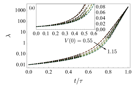
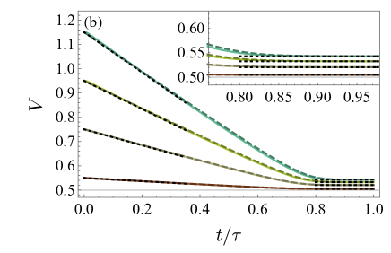
Figure 1: The optimal control of isothermal processes in generic damped situation. (a) The optimal protocols with different control speeds characterized by $V(0)=0.55$, $0.75$, $0.95$, and $1.15$. We plot all the protocols (dashed curves) with a rescaled time $t/\tau$ with $\lambda(0)=0.01$ and $\lambda(\tau)=2000$. (b) The evolution of the potential energy $V$ during the isothermal processes. The solid curves show the results of exact evolution by Eqs. (3)-(5). In both subfigures, the dotted lines show the results in the overdamped and the underdamped limits, and the dashed curves are the results of the approximate dynamics obtained from Eqs. (8) and (16).

After solving the protocols from Eqs. (8) and (16), we can utilize these protocols to propagate the exact evolution of nonquasistatic isothermal processes by Eqs. (3)-(5). The results are compared and visualized in Fig. 1. We set the bath temperature $T_{b}=1$, the friction coefficient $\kappa=1$, and the initial and final values of stiffness $\lambda(0)=0.01$ and $\lambda(\tau)=2000$, and choose four initial values of the potential energy $V(0)=0.55$, $0.75$, $0.95$, and $1.15$. With larger $V(0)$, the isothermal compression is completed more rapidly. Figure 1(a) shows the control protocols of the stiffness $\lambda(t)$ (dashed curves). The black dotted curves represent the optimal protocols in the overdamped limit (Schmiedl and Seifert, 2007a, b) and the underdamped limit (Dechant et al., 2017; Chen et al., 2022), matching our protocols at the initial and final stages, respectively. Figure 1(b) shows the evolution of potential energy during isothermal compression processes. The dashed curves are the estimations based on the approximate dynamics, while the solid curves show the exact evolution by Eqs. (3)-(5) with the protocols in Fig. 1(a). The agreement of the solid curves and the dashed curves validates the approximation used in Eq. (7).

Construction of the optimal cycles. We continue to construct heat-engine cycles under the control constraints $\lambda_{L}\leq\lambda\leq\lambda_{H}$ and $T_{L}\leq T_{b}\leq T_{H}$. During the whole cycle, the pseudo Hamiltonian is conserved and we thus require two isothermal processes with identical $\mathcal{H}$. For given $\mathcal{H}$, we find two switchings associated with the lower and the upper stiffness constraints $\lambda_{L}$ and $\lambda_{H}$ by simultaneously changing $T_{b}$ and $\lambda$ (Sup, ). Thus, $\mathcal{H}$ together with the control constraints determines the control protocol of the cycle.

The switchings simultaneously change $\lambda$ and $T_{b}$ instantaneously, i.e., $\alpha\gg\kappa$, and the evolution equations (8) and (10) are reduced to

$$\dot{V} =\frac{\kappa^{2}+\lambda}{\kappa^{2}+2\lambda}\alpha V,$$ (23)

$$\dot{\psi}_{V} =\alpha\left[1-\frac{\left(\kappa^{2}+\lambda\right)}{\kappa^{2}+2\lambda}\psi_{V}\right].$$ (24)

The initial and the final points of the switchings satisfy

$$\frac{V_{f}\sqrt{\kappa^{2}+2\lambda_{f}}}{\lambda_{i}} =\frac{V_{i}\sqrt{2\lambda_{i}+\kappa^{2}}}{\lambda_{i}},$$ (25)

$$\frac{\lambda_{f}(\psi_{Vf}-2)-\kappa^{2}}{\sqrt{\kappa^{2}+2\lambda_{f}}} =\frac{\lambda_{i}\left(\psi_{Vi}-2\right)-\kappa^{2}}{\sqrt{\kappa^{2}+2\lambda_{i}}}.$$ (26)

The two switchings in a cycle are given by $\lambda_{2}\rightarrow\lambda_{H},V_{2}\rightarrow V_{3},\psi_{V2}\rightarrow\psi_{V3}$ and $\lambda_{5}\rightarrow\lambda_{L},V_{5}\rightarrow V_{6},\psi_{V5}\rightarrow\psi_{V6}$, as shown in Fig. 2(a). The six boundary points are $l=1,2,...,6$, and the six processes I, II, …, VI. The two switchings are solved from the conservation of $\mathcal{H}$ (Sup, ). With $\mathcal{H}$ large enough, the lower switching connects the two isothermal processes directly without reaching the lower stiffness constraint $\lambda_{L}$. By increasing $\mathcal{H}$, point 6 will approach point 1 on the cold isothermal curve. Since larger $\mathcal{H}$ leads to higher output power, we consider the maximum $\mathcal{H}$ such that the cycle still reaches $\lambda_{L}$. The output power $P$ of the maximum-$\mathcal{H}$ cycle is evaluated as

$$P=-\frac{W_{\mathrm{I}}+W_{\mathrm{II}}+W_{\mathrm{IV}}+W_{\mathrm{V}}}{\tau_{\mathrm{I}}+\tau_{\mathrm{III}}+\tau_{\mathrm{IV}}}.$$ (27)

The expressions of the work and the operation time of each process are given in (Sup, ).

With the above protocol of a whole cycle, we can propagate Eqs. (3)-(5) and obtain the exact output power of the limit cycle. In accordance with Eq. (27), we choose the connecting processes to be thermodynamic adiabatic (unitary) processes that satisfy $\Gamma_{pp}^{f}\Gamma_{xx}^{f}=\Gamma_{pp}^{i}\Gamma_{xx}^{i}$. In principle, such unitary evolution can be completed in arbitrary short time by choosing a large Hamiltonian (Mandelstam and Tamm, 1945; Margolus and Levitin, 1998). The corresponding protocol to vary the Hamiltonian can be realized by the shortcut to adiabaticity (Berry, 2009; Guéry-Odelin et al., 2019). After solving $\Gamma_{xx}$, $\Gamma_{xp}$, and $\Gamma_{pp}$ for the whole cycle, we also use Eq. (27) to evaluate the exact output power, where the work in each process is evaluated from the exact evolution.

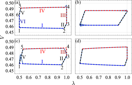
Figure 2: Diagrams of heat-engine cycles. (a) $\kappa=1$ and $\mathcal{H}=10^{-4}$ (non-maximum $\mathcal{H}$), (b) $\kappa=0.1$ (underdamped), (c) $\kappa=0.830$ (optimal), and (d) $\kappa=10$ (overdamped). The control constraints $T_{L}=0.9$, $T_{H}=1$, $\lambda_{L}=0.5$ and $\lambda_{H}=1$ are depicted by the horizontal and vertical gray lines. The solid and the dashed curves represent limit cycles of the exact dynamics and the approximate dynamics, respectively.

We show diagrams of heat-engine cycles in Fig. 2 for a non-maximum-$\mathcal{H}$ cycle with (a) $\kappa=1$ and $\mathcal{H}=10^{-4}$, and three maximum-$\mathcal{H}$ cycles with (b) $\kappa=0.1$ (underdamped), (c) $\kappa=0.830$ (optimal), and (d) $\kappa=10$ (overdamped). Although the exact evolution (solid curves) deviates from the evolution based on the approximate dynamics (dashed curves), our protocols still lead to high output power in the intermediate coupling regime. In the underdamped limit (Fig. 2(b)), the microscopic heat engine fulfills all the preconditions of the Curzon-Ahlborn engine (Curzon and Ahlborn, 1975; Chen et al., 2022), where the effective temperature of the Brownian particle remains constant ($V=\mathrm{const}$) during isothermal processes (Curzon and Ahlborn, 1975; Chen et al., 2022).

Maximum power of Brownian heat engines. For a given friction coefficient $\kappa$, we evaluate the output power $P$ of maximum-$\mathcal{H}$ cycles. Furthermore, the friction coefficient $\kappa$ can be adjusted to achieve the maximum power. In generic damped situation, we solve the maximum-$\mathcal{H}$ cycle numerically. Analytical results are obtained in the overdamped limit and the underdamped limit.

In the overdamped limit $\kappa^{2}\gg\lambda_{H}$, the cooling rate according to Eq. (8) is equal to $2\lambda/\kappa$. Thus, the output power is inversely proportional to the friction coefficient $P_{\mathrm{over}}\propto 1/\kappa$ (Sup, ). We can choose $\lambda_{L}$ as large as possible so that the maximum power $P_{\mathrm{over}}^{*}$ can be achieved by the sliced cycles (Sup, )

$$P_{\mathrm{over}}^{*}=\frac{\lambda_{H}T_{H}}{\kappa}\phi(\frac{T_{L}}{T_{H}}),$$ (28)

where $\phi(\theta)$ is the positive root of the polynomial

$$\phi^{3}+(11-3\theta)\phi^{2}+\left(3\theta^{2}+14\theta-1\right)\phi-(\theta-1)^{2}\theta=0,$$ (29)

with $\theta=T_{L}/T_{H}$. A detailed discussion of these sliced cycles is left in (Sup, ).

In the underdamped limit $\kappa^{2}\ll\lambda_{L}$, the maximum power is (Dechant et al., 2017; Chen et al., 2022)

$$P_{\mathrm{under}}^{*}=\frac{\kappa T_{H}}{4}(1-\sqrt{\frac{T_{L}}{T_{H}}})^{2},$$ (30)

which is proportional to the square of the Curzon-Ahlborn efficiency $\eta_{\mathrm{CA}}=1-\sqrt{T_{L}/T_{H}}$ (Curzon and Ahlborn, 1975). We left the derivations of Eqs. (28) and (30) in (Sup, ).

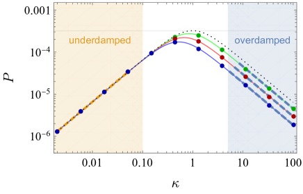
Figure 3: Output power of the optimal cycles with different friction coefficients. We fix the parameters $T_{L}=0.9$, $T_{H}=1$, $\lambda_{H}=1$, and choose different lower stiffness constraints $\lambda_{L}=1/8$ (blue), $1/4$ (red), $1/2$ (green). The dots and the solid curves show the results of the exact dynamics [Eqs. (3)-(5)] and the approximate dynamics [Eq. (8)], respectively. The maximum power in the overdamped and the underdamped limits is shown with the right and left dashed lines. The dotted curve show the maximum power of sliced cycles, and the gray horizontal line shows the bound of the output power $P_{\mathrm{bound}}$ with the appropriate friction coefficient.

Figure 3 presents the output power $P$ of maximum-$\mathcal{H}$ cycles as a function of the friction coefficient $\kappa$. We set the control constraints $T_{H}=1$, $T_{L}=0.9$, and $\lambda_{H}=1$, and choose the lower stiffness constraint $\lambda_{L}=1/8$ (blue), $1/4$ (red), $1/2$ (green). The output power of the exact dynamics (dots) agrees well with that of the approximate dynamics (solid curves), and is bounded by the maximum power of sliced cycles (dotted curve) (Sup, ). The maximum power of sliced cycles agrees with Eqs. (28) and (30) in the overdamped and the underdamped limits. The gray horizontal line shows the bound of the output power $P_{\mathrm{bound}}$ with the appropriate friction coefficient which leads to the maximum power (Sup, ).

Conclusion. The maximum power of Brownian heat engines in the overdamped and the underdamped limits has been obtained previously (Schmiedl and Seifert, 2007a, b; Dechant et al., 2017; Chen et al., 2022), but how to reach the maximum power in the intermediate coupling regime (generic damped situation) has been a long-standing problem. Previous methods fail in this regime due to the lack of timescale separation.

In our current investigation, we have employed the optimal control theory to study the performance of Brownian heat engines to achieve the maximum power. We construct the optimal cycles in generic damped situation. These optimal cycles include two isothermal processes, two adiabatic processes, and an extra isochoric relaxation process at the upper stiffness constraint. We also determine appropriate friction coefficient to achieve the maximum power. This indicates that powerful thermal engines operate at the intermediate coupling regime, neither the weak coupling regime (underdamped limit) nor the strong coupling regime (overdamped limit). This argument should also be valid for quantum heat engines (Uzdin et al., 2016; Gelbwaser-Klimovsky and Aspuru-Guzik, 2015; Perarnau-Llobet et al., 2018).

Our findings show the effectiveness of the optimal control theory in thermodynamic optimization, and provide practical guidance for the experimental design and optimization of Brownian heat engines. It is interesting to explore the trade-off relation between the efficiency and output power of Brownian heat engines in generic damped situation and also the optimal protocol of cycles to achieve the maximum power at a given efficiency (Abiuso and Perarnau-Llobet, 2020; Chen and Yan, 1989; Shiraishi et al., 2016; Pietzonka and Seifert, 2018; Ma et al., 2018; Holubec and Ryabov, 2016), and we leave this for future investigation.

Acknowledgment. This work is supported by the National Natural Science Foundation of China (NSFC) under Grants No. 12147157, No. 11775001 and No. 11825501, No. 12375028.

References

- Blickle and Bechinger (2012) V. Blickle and C. Bechinger, Realization of a micrometre-sized stochastic heat engine, Nat. Phys. 8, 143 (2012).
- Quinto-Su (2014) P. A. Quinto-Su, A microscopic steam engine implemented in an optical tweezer, Nat. Commun. 5, 5889 (2014).
- Martínez et al. (2016) I. A. Martínez, É. Roldán, L. Dinis, D. Petrov, J. M. R. Parrondo, and R. A. Rica, Brownian Carnot engine, Nat. Phys. 12, 67 (2016).
- Krishnamurthy et al. (2016) S. Krishnamurthy, S. Ghosh, D. Chatterji, R. Ganapathy, and A. K. Sood, A micrometre-sized heat engine operating between bacterial reservoirs, Nat. Phys. 12, 1134 (2016).
- Martínez et al. (2017) I. A. Martínez, É. Roldán, L. Dinis, and R. A. Rica, Colloidal heat engines: a review, Soft Matter 13, 22 (2017).
- Holubec and Ryabov (2021) V. Holubec and A. Ryabov, Fluctuations in heat engines, J. Phys. A: Math. Theor. 55, 013001 (2021).
- Schmiedl and Seifert (2007a) T. Schmiedl and U. Seifert, Optimal finite-time processes in stochastic thermodynamics, Phys. Rev. Lett. 98, 108301 (2007a).
- Schmiedl and Seifert (2007b) T. Schmiedl and U. Seifert, Efficiency at maximum power: An analytically solvable model for stochastic heat engines, Europhys. Lett. 81, 20003 (2007b).
- Zulkowski and DeWeese (2015) P. R. Zulkowski and M. R. DeWeese, Optimal control of overdamped systems, Phys. Rev. E 92, 032117 (2015).
- Plata et al. (2019) C. A. Plata, D. Guéry-Odelin, E. Trizac, and A. Prados, Optimal work in a harmonic trap with bounded stiffness, Phys. Rev. E 99, 012140 (2019).
- Proesmans et al. (2020) K. Proesmans, J. Ehrich, and J. Bechhoefer, Finite-Time Landauer Principle, Phys. Rev. Lett. 125, 100602 (2020).
- Ye et al. (2022) Z. Ye, F. Cerisola, P. Abiuso, J. Anders, M. Perarnau-Llobet, and V. Holubec, Optimal finite-time heat engines under constrained control, Phys. Rev. Research 4, 043130 (2022).
- Xu et al. (2022) G.-H. Xu, C. Jiang, Y. Minami, and G. Watanabe, Relation between fluctuations and efficiency at maximum power for small heat engines, Phys. Rev. Research 4, 043139 (2022).
- Dechant et al. (2017) A. Dechant, N. Kiesel, and E. Lutz, Underdamped stochastic heat engine at maximum efficiency, Europhys. Lett. 119, 50003 (2017).
- Chen et al. (2022) Y. H. Chen, J.-F. Chen, Z. Fei, and H. T. Quan, Microscopic theory of the Curzon-Ahlborn heat engine based on a Brownian particle, Phys. Rev. E 106, 024105 (2022).
- Curzon and Ahlborn (1975) F. L. Curzon and B. Ahlborn, Efficiency of a Carnot engine at maximum power output, Am. J. Phys 43, 22 (1975).
- Salamon and Berry (1983) P. Salamon and R. S. Berry, Thermodynamic Length and Dissipated Availability, Phys. Rev. Lett. 51, 1127 (1983).
- Crooks (2007) G. E. Crooks, Measuring Thermodynamic Length, Phys. Rev. Lett. 99, 100602 (2007).
- Sivak and Crooks (2012) D. A. Sivak and G. E. Crooks, Thermodynamic Metrics and Optimal Paths, Phys. Rev. Lett. 108, 190602 (2012).
- Zulkowski et al. (2012) P. R. Zulkowski, D. A. Sivak, G. E. Crooks, and M. R. DeWeese, Geometry of thermodynamic control, Phys. Rev. E 86, 041148 (2012).
- Scandi and Perarnau-Llobet (2019) M. Scandi and M. Perarnau-Llobet, Thermodynamic length in open quantum systems, Quantum 3, 197 (2019).
- Cavina et al. (2017) V. Cavina, A. Mari, and V. Giovannetti, Slow Dynamics and Thermodynamics of Open Quantum Systems, Phys. Rev. Lett. 119, 050601 (2017).
- Brandner and Saito (2020) K. Brandner and K. Saito, Thermodynamic Geometry of Microscopic Heat Engines, Phys. Rev. Lett. 124, 040602 (2020).
- Chen et al. (2021) J.-F. Chen, C. P. Sun, and H. Dong, Extrapolating the thermodynamic length with finite-time measurements, Phys. Rev. E 104, 034117 (2021).
- Abiuso and Perarnau-Llobet (2020) P. Abiuso and M. Perarnau-Llobet, Optimal Cycles for Low-Dissipation Heat Engines, Phys. Rev. Lett. 124, 110606 (2020).
- Li et al. (2022) G. Li, J.-F. Chen, C. P. Sun, and H. Dong, Geodesic Path for the Minimal Energy Cost in Shortcuts to Isothermality, Phys. Rev. Lett. 128, 230603 (2022).
- Chen (2022) J.-F. Chen, Optimizing Brownian heat engine with shortcut strategy, Phys. Rev. E 106, 054108 (2022).
- Frim and DeWeese (2022) A. G. Frim and M. R. DeWeese, Geometric Bound on the Efficiency of Irreversible Thermodynamic Cycles, Phys. Rev. Lett. 128, 230601 (2022).
- Wang and Ren (2023) Z. Wang and J. Ren, Thermodynamic Geometry of Nonequilibrium Fluctuations in Cyclically Driven Transport, (2023), 10.48550/ARXIV.2304.08181, arXiv:2304.08181 [cond-mat.stat-mech] .
- Pontryagin et al. (1962) L. S. Pontryagin, V. G. Boltyanskii, R. V. Gamkrelidze, and E. F. Mishechenko, The Mathematical Theory of Optimal Processes (Wiley, New York, 1962).
- Peirce et al. (1988) A. P. Peirce, M. A. Dahleh, and H. Rabitz, Optimal control of quantum-mechanical systems: Existence, numerical approximation, and applications, Phys. Rev. A 37, 4950 (1988).
- Caneva et al. (2009) T. Caneva, M. Murphy, T. Calarco, R. Fazio, S. Montangero, V. Giovannetti, and G. E. Santoro, Optimal Control at the Quantum Speed Limit, Phys. Rev. Lett. 103, 240501 (2009).
- Lloyd and Montangero (2014) S. Lloyd and S. Montangero, Information Theoretical Analysis of Quantum Optimal Control, Phys. Rev. Lett. 113, 010502 (2014).
- Li et al. (2017) J. Li, X. Yang, X. Peng, and C.-P. Sun, Hybrid Quantum-Classical Approach to Quantum Optimal Control, Phys. Rev. Lett. 118, 150503 (2017).
- Boscain et al. (2021) U. Boscain, M. Sigalotti, and D. Sugny, Introduction to the Pontryagin Maximum Principle for Quantum Optimal Control, PRX Quantum 2, 030203 (2021).
- Yang et al. (2017) Z.-C. Yang, A. Rahmani, A. Shabani, H. Neven, and C. Chamon, Optimizing Variational Quantum Algorithms Using Pontryagin’s Minimum Principle, Phys. Rev. X 7, 021027 (2017).
- Brady et al. (2021) L. T. Brady, C. L. Baldwin, A. Bapat, Y. Kharkov, and A. V. Gorshkov, Optimal Protocols in Quantum Annealing and Quantum Approximate Optimization Algorithm Problems, Phys. Rev. Lett. 126, 070505 (2021).
- Rubin (1979) M. H. Rubin, Optimal configuration of a class of irreversible heat engines. II, Phys. Rev. A 19, 1277 (1979).
- Cavina et al. (2018) V. Cavina, A. Mari, A. Carlini, and V. Giovannetti, Optimal thermodynamic control in open quantum systems, Phys. Rev. A 98, 012139 (2018).
- Kramers (1940) H. Kramers, Brownian motion in a field of force and the diffusion model of chemical reactions, Physica 7, 284 (1940).
- Rezek and Kosloff (2006) Y. Rezek and R. Kosloff, Irreversible performance of a quantum harmonic heat engine, New J. Phys. 8, 83 (2006).
- Chen and Quan (2023) J.-F. Chen and H. T. Quan, Hierarchical structure of fluctuation theorems for a driven system in contact with multiple heat reservoirs, Phys. Rev. E 107, 024135 (2023).
- (43) Supplementary Materials, .
- Gong et al. (2016) Z. Gong, Y. Lan, and H. Quan, Stochastic Thermodynamics of a Particle in a Box, Phys. Rev. Lett. 117, 180603 (2016).
- Salazar (2020) D. S. P. Salazar, Work distribution in thermal processes, Phys. Rev. E 101, 030101 (2020).
- Mandelstam and Tamm (1945) L. Mandelstam and I. G. Tamm, The uncertainty relationbetween energy and time in nonrelativistic quantum mechanics, J. Phys. USSR 9, 249 (1945).
- Margolus and Levitin (1998) N. Margolus and L. B. Levitin, The maximum speed of dynamical evolution, Phys. D: Nonlinear Phenom. 120, 188 (1998).
- Berry (2009) M. V. Berry, Transitionless quantum driving, J. Phys. A: Math. Theor. 42, 365303 (2009).
- Guéry-Odelin et al. (2019) D. Guéry-Odelin, A. Ruschhaupt, A. Kiely, E. Torrontegui, S. Martínez-Garaot, and J. G. Muga, Shortcuts to adiabaticity: Concepts, methods, and applications, Rev. Mod. Phys. 91, 045001 (2019).
- Uzdin et al. (2016) R. Uzdin, A. Levy, and R. Kosloff, Quantum Heat Machines Equivalence, Work Extraction beyond Markovianity, and Strong Coupling via Heat Exchangers, Entropy 18, 124 (2016).
- Gelbwaser-Klimovsky and Aspuru-Guzik (2015) D. Gelbwaser-Klimovsky and A. Aspuru-Guzik, Strongly Coupled Quantum Heat Machines, J. Phys. Chem. Lett. 6, 3477 (2015).
- Perarnau-Llobet et al. (2018) M. Perarnau-Llobet, H. Wilming, A. Riera, R. Gallego, and J. Eisert, Strong Coupling Corrections in Quantum Thermodynamics, Phys. Rev. Lett. 120, 120602 (2018).
- Chen and Yan (1989) L. Chen and Z. Yan, The effect of heat-transfer law on performance of a two-heat-source endoreversible cycle, J. Chem. Phys. 90, 3740 (1989).
- Shiraishi et al. (2016) N. Shiraishi, K. Saito, and H. Tasaki, Universal trade-off relation between power and efficiency for heat engines, Phys. Rev. Lett. 117, 190601 (2016).
- Pietzonka and Seifert (2018) P. Pietzonka and U. Seifert, Universal trade-off between power, efficiency, and constancy in steady-state heat engines, Phys. Rev. Lett. 120, 190602 (2018).
- Ma et al. (2018) Y.-H. Ma, D. Xu, H. Dong, and C.-P. Sun, Universal constraint for efficiency and power of a low-dissipation heat engine, Phys. Rev. E 98, 042112 (2018).
- Holubec and Ryabov (2016) V. Holubec and A. Ryabov, Maximum efficiency of low-dissipation heat engines at arbitrary power, J. Stat. Mech: Theory Exp. 2016, 073204 (2016).