Technical Report on the Learning of Case Relevance in Case-Based Reasoning with Abstract Argumentation

Abstract

Case-based reasoning is known to play an important role in several legal settings. In this paper we focus on a recent approach to case-based reasoning, supported by an instantiation of abstract argumentation whereby arguments represent cases and attack between arguments results from outcome disagreement between cases and a notion of relevance. We explore how relevance can be learnt automatically in practice with the help of decision trees, and explore the combination of case-based reasoning with abstract argumentation (${AA\mathchar 45\relax CBR}$) and learning of case relevance for prediction in legal settings. Specifically, we show that, for two legal datasets, ${AA\mathchar 45\relax CBR}$ and decision-tree-based learning of case relevance perform competitively in comparison with decision trees. We also show that ${AA\mathchar 45\relax CBR}$ with decision-tree-based learning of case relevance results in a more compact representation than their decision tree counterparts, which could be beneficial for obtaining cognitively tractable explanations.

and

1 Introduction

Case-based reasoning (CBR) is a methodology in which concrete past occasions are directly used as sources of knowledge and solutions for new situations (DBLP:books/daglib/0032926, ). It has been studied in AI and Law since its inception, leading to foundational contributions (Rissland2005CasebasedRA, ). This is a not a surprise, given the centrality of the use of cases for determining the law in Common Law systems, although not exclusively lewis2021 .

In this paper we focus on recent approaches to CBR (DBLP:conf/kr/CyrasST16, ; dear-2020, ; DBLP:conf/kr/Paulino-PassosT21, ; Prakken2022ATM, ) using argumentation (prakken-overview, ). Argumentation itself has a long history in AI and Law, and its use to support CBR has been shown to pave the way towards novel forms of explanations for the outcomes of CBR, including via arbitrated dispute trees (DBLP:journals/eswa/CyrasBGTDTGH19, ; DBLP:conf/ijcai/Cyras0ABT21, ). Specifically, we focus on the ${AA\mathchar 45\relax CBR}$ approach (DBLP:conf/kr/CyrasST16, ; dear-2020, ; DBLP:conf/kr/Paulino-PassosT21, ), where arguments correspond to cases and attacks between arguments result from outcome disagreement between cases and relevance between cases, guided by a partial order over cases capturing some notion of specificity. Originally (DBLP:conf/kr/CyrasST16, ), ${AA\mathchar 45\relax CBR}$ expects a representation of cases in terms of sets of manually engineered binary features and the partial order is defined via the subset relation. This expectation is a restriction for applicability. While previous work has generalised beyond binary features in order to support different applications dear-2020 , a systematic generalisation to tabular datasets, including categorical and continuous data, is still missing. This is essential for applying ${AA\mathchar 45\relax CBR}$ to realistic datasets, including legal ones, to realise the original inspiration from legal reasoning for ${AA\mathchar 45\relax CBR}$. While some form of binarisation can be applied, there is no guarantee that a naïve binarisation would result in good performance. In this work we close this gap, focusing on applying ${AA\mathchar 45\relax CBR}$ to possibly non-binary tabular data from legal settings.

Specifically, our first contribution is a general method for applying ${AA\mathchar 45\relax CBR}$ to any tabular data by extracting binary features from decision trees DBLP:books/wa/BreimanFOS84 when learning for the final task. Our second contribution is showing that this method is competitive with decision trees on two legal datasets: COMPAS propublica-compas and a simulated legal dataset DBLP:journals/argcom/StegingRVB23 for welfare benefit. Finally, as a third contribution, we show that our method creates smaller models (i.e. with a smaller number of nodes), leading to potentially more cognitively tractable explanations (i.e. decision trees and rules drawn from them on one hand, and argumentation frameworks and arbitrated dispute trees on the other).

2 Background

Abstract Argumentation frameworks (AFs).

An AF Dung:95 is a pair $(\mathit{Args},\leadsto)$, where $\mathit{Args}$ is a set (of arguments) and $\leadsto$$\subseteq\!\!\mathit{Args}\!\times\!\mathit{Args}$ is a binary relation (of attack) on $\mathit{Args}$. For $\alpha,\beta\!\in\!\mathit{Args}$, if $\alpha\!\leadsto\!\beta$, then we say that $\alpha$ attacks $\beta$. $E\!\subseteq\!\mathit{Args}$ defends $\alpha\!\in\!\mathit{Args}$ if for all $\beta\!\leadsto\!\alpha$ there exists $\gamma\!\in\!E$ such that $\gamma\!\leadsto\!\beta$. The grounded extension of $(\mathit{Args},\leadsto)$ is $\mathbb{G}\!=\!\bigcup_{i\geqslant 0}G_{i}$, where $G_{0}$ is the set of all unattacked arguments, and $\forall i\!\geqslant\!0$, $G_{i+1}$ is the set of arguments that $G_{i}$ defends.

Abstract Argumentation for Case-Based Reasoning (${AA\mathchar 45\relax CBR}$).

We use the ${AA\mathchar 45\relax CBR}_{\succeq}$ presentation from DBLP:conf/kr/Paulino-PassosT21 . Let $X$ be a set of characterisations, equipped with partial order $\preceq$. Let $Y\!=\!\{\delta_{o},\bar{\delta_{o}}\}$ be a set of outcomes, with $\delta_{o}$ the default outcome. We discriminate a particular element $\delta_{C}\!\in\!X$ such that $\delta_{C}$ is the $\preceq$-minimum element of $X$ and define the default argument ${\small\mbox{$(\delta_{C},\delta_{o})$}}\!\in\!X\!\times\!Y$. A casebase (aka dataset) $D$ is a finite $D\!\subseteq\!X\!\times\!Y$, consisting of past cases (aka labelled examples) $\alpha\in D$ is of the form $(\alpha_{C},\alpha_{o})$ for $\alpha_{C}\!\in\!X$, $\alpha_{o}\!\in\!Y$. Instead, a new case (aka unlabelled example) is of the form $({N}_{C},?)$ for ${N_{C}}\!\in\!X$.

The partial order $\preceq$ defines a notion of relevance $\sim$ between characterisations, where $x_{1}\!\sim{}\!x_{2}$ iff $x_{2}\!\preceq\!x_{1}$. This notion and crucially irrelevance (defined as $\not\sim$) are used to compare new and past cases as well as two past cases. (thus in ${AA\mathchar 45\relax CBR}_{\succeq}$ relevance is not symmetric). The idea is that the partial order $\preceq$ captures specificity between cases, and that the outcome for a new case depends only on past cases than which the new case is more specific. For simplicity, we extend the definition of $\succeq$ (and $\nsim$) to cases by setting ${\small\mbox{$(\alpha_{c},\alpha_{o})$}}\succeq{\small\mbox{$(\beta_{c},\beta_{o})$}}$ iff $\alpha_{c}\succeq\beta_{c}$ (and ${\small\mbox{$({N}_{C},?)$}}\!\!\not\sim\!\!(\beta_{C},\!\beta_{o})$ iff ${N_{C}}\ \!\!\not\sim\!\!\beta_{C}$). For characterisations as sets of binary features, as in (DBLP:conf/kr/CyrasST16, ), $\succeq=\supseteq$ captures specificity.

A casebase $D$ is coherent iff there are no two cases ${\small\mbox{$(\alpha_{C},\alpha_{o})$}},{\small\mbox{$(\beta_{C},\beta_{o})$}}\in D$ such that $\alpha_{C}=\beta_{C}$ but $\alpha_{o}\neq\beta_{o}$, and it is incoherent otherwise.

The AF mined from a dataset $D$ and a new case $({N}_{C},?)$, given default argument $(\delta_{C},\delta_{o})$, is $(\mathit{Args},\leadsto)$ (referred to as $AF_{\succeq}(D,{N_{C}})$ later), in which:

1. $\mathit{Args}=D\cup\{{\small\mbox{$(\delta_{C},\delta_{o})$}}\}\cup\{{\small\mbox{$({N}_{C},?)$}}\}$;

2. for $(\alpha_{C},\alpha_{o})\in D$, $(\beta_{C},\beta_{o})\in D\cup\{{\small\mbox{$(\delta_{C},\delta_{o})$}}\}$, it holds that $(\alpha_{C},\alpha_{o})\leadsto(\beta_{C},\beta_{o})$ iff

   (a) $\alpha_{o}\neq\beta_{o}$,  (b) $\alpha_{C}\succeq\beta_{C}$,  and

   (c) $\nexists(\gamma_{C},\gamma_{o})\in D\cup\{{\small\mbox{$(\delta_{C},\delta_{o})$}}\}$ with $\alpha_{C}\succ\gamma_{C}\succ\beta_{C}$ and $\gamma_{o}=\alpha_{o}$;

3. for $(\beta_{C},\!\beta_{o})\!\!\in\!\!D\cup\!\{\!{\small\mbox{$(\delta_{C},\delta_{o})$}}\!\}$, it holds that ${\small\mbox{$({N_{C}},?)$}}\!\!\leadsto\!\!(\beta_{C},\!\beta_{o})$ iff ${\small\mbox{$({N}_{C},?)$}}\!\!\not\sim\!\!(\beta_{C},\!\beta_{o})$.

Let $\mathbb{G}$ be the grounded extension of $AF_{\succeq}(D,{N_{C}})$. Then, the outcome for ${N_{C}}$ is $\delta_{o}$ if $(\delta_{C},\delta_{o})$ is in $\mathbb{G}$, and $\bar{\delta_{o}}$ otherwise.

In the remainder, we will also use the notion of AF mined from a dataset $D$ alone (referred to as $AF_{\succeq}(D)$), amounting to $(\mathit{Args}^{\prime},\leadsto^{\prime})$ with $\mathit{Args}^{\prime}=\mathit{Args}\setminus\{{\small\mbox{$({N}_{C},?)$}}\}$ and $\leadsto^{\prime}=\leadsto\cap(\mathit{Args}^{\prime}\times\mathit{Args}^{\prime})$ where $AF_{\succeq}(D,{N_{C}})$=$(\mathit{Args},\leadsto)$. Besides experimenting with (learnt instances of) ${AA\mathchar 45\relax CBR}_{\succeq}$, we will also experiment with the cumulative version thereof ($c{{AA\mathchar 45\relax CBR}_{\succeq}}$) from (DBLP:conf/kr/Paulino-PassosT21, ) (definition omitted for lack of space). Finally, we will use arbitrated dispute trees (ADT) as explanations DBLP:journals/eswa/CyrasBGTDTGH19 . Intuitively, ADTs capture a debate in which, if the classification is the default outcome, then the winner successfully defends every attacker of the default argument, and otherwise the winner presents a successful attack to the default argument (example in Figure 1) .

Figure 1: ADT originated from a ${AA\mathchar 45\relax CBR}_{\succeq}$ model trained on the Welfare dataset. Nodes are labelled as follows: whether winning ($\mathbf{W}$) or losing ($\mathbf{L}$); feature values of the case for: age, paid_contribution5, is_spouse, is_absent, capital_resources; the set of features extracted from the decision tree splits; the case outcome (“$+$” for eligible, “$-$” for ineligible, and “$?$” for new case).

3 Learning Relevance

Learning relevance in ${AA\mathchar 45\relax CBR}_{\succeq}$ amounts to learning the partial order $\succeq$, which represents specificity. We can think of it in terms of the 4R cycle of CBR: retrieve, reuse, revise, and retain DBLP:books/daglib/0032926 . Retrieval is determined by (ir)relevance, which in turn is determined by the partial order. Reuse of solutions depend on the structure of the AF mined from the data, which again depends exclusively on case characterisation and on the partial order. Assuming revision to be external (e.g. by human or environmental feedback), then finally retaining is also dependent on the partial order, since retaining is nothing more than adding into the mined AF, which is also determined by the partial order.

Here we use decision tree learning, a classic and widely used machine learning method, to extract characterisations suitable for ${AA\mathchar 45\relax CBR}_{\supseteq}$ (i.e. ${AA\mathchar 45\relax CBR}_{\succeq}$ with $\succeq=\supseteq$) from tabular data, regardless of the nature of features therein. Specifically, we use the algorithm CART for learning decision trees, in which decision nodes are greedily created choosing the feature and the split threshold which minimises some loss function: those splits result in a binary divide between examples which are below the split threshold and the ones above; each split can then be seen as a binary feature, and each example can be characterised simply as a set of binary features, that is, the set of split rules for which the example is below the threshold. Specificity here then simply means having all (binary) features of another case. The following example provides a simple illustration of our method.

Example 1.

Consider the dataset with the following labelled examples:

$$\alpha ={\small\mbox{$((\text{age}=20,\text{prior\_count}=2),\texttt{+})$}}, \gamma ={\small\mbox{$((\text{age}=35,\text{prior\_count}=7),\texttt{+})$}},$$

$$\beta ={\small\mbox{$((\text{age}=30,\text{prior\_count}=1),\texttt{-})$}}, \epsilon ={\small\mbox{$((\text{age}=19,\text{prior\_count}=1),\texttt{-})$}},$$

$$\eta ={\small\mbox{$((\text{age}=19,\text{prior\_count}=10),\texttt{+})$}}$$

Assume as well the decision tree on the left of Figure 2 was trained on this dataset. Assume further that the default outcome for ${AA\mathchar 45\relax CBR}_{\succeq}$is $+$, reflecting that the majority of the dataset has the output recid. Then, on the right of Figure 2 we show $AF_{\succeq}(D)$, the AF mined from the dataset $D$ obtained from the original dataset by binarising features: each example in the original dataset is represented by the split tests for which it is evaluated true. The resulting $D$ is then used as a casebase for ${AA\mathchar 45\relax CBR}_{\supseteq}$. Notice how there is no bijection between leaves in the decision tree and cases in the AF. The correspondence is one to many, since examples falling into the same leaf may correspond to different cases in the AF. For example, see how the rightmost leaf corresponds to $(\{\texttt{age\_<=\_21}\},+)$ (via case $\eta$), to $(\{\texttt{age\_<=\_21},\texttt{prior\_count\_<=\_3}\},+)$ (via case $\alpha$), and finally to $(\{\texttt{age\_<=\_21},\texttt{prior\_count\_<=\_3}\},-)$ (via case $\epsilon$). Notice also that there is no case $(\{\},-)$ resulting from the splits, since the only cases with no features has the recid outcome (had there been such a case then it would have been a better choice for the default argument). Also, when multiple cases would have the same characterisation but different outcomes, either an incoherence is generated, or it is avoided via preprocessing. Here we illustrate an incoherence occurring.

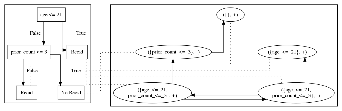
Figure 2: On the left, decision tree learnt from the dataset in Example 1. On the right, $AF_{\succeq}(D)$ for $D$ drawn from the splits in the decision tree. Dotted lines indicate correspondence between a leaf node on the left and a case on the right.

4 Experiments

We train decision trees with pre-pruning, that is, limiting maximum depth and maximum number of leaf nodes for the decision tree as a regularisation, where the best maximum vales are hyperparameters chosen by cross-validation. We used the following set of values: for maximum depth, varying from 3 to 13, in a step of 2; for maximum number of leaf nodes, from 4 to 512, in geometric progression of ratio 2. Nodes are greedily created in a best-first search fashion, using Gini impurity as the criterion. We evaluate three approaches for the problem of incoherence: 1. keep: to keep the incoherence and letting each model deal with this in their own ways; 2. removal: to remove every incoherent pair of cases; 3. majority: for each characterisation in the resulting transformation, count the number of training examples corresponding to each output and select the majority output as the outcome for the (now unique) case.

4.1 COMPAS Dataset

The first dataset we use is COMPAS, which contains predicted scores of recidivism and data of actual (measured) recidivism (propublica-compas, ). The COMPAS dataset is based on a proprietary prediction model for recidivism widely used in the U.S (propublica-compas, ) and it has been the focus of much work on algorithmic biases and impact of technology in the justice system. Our goal is not evaluating the COMPAS algorithm or discuss its fairness (propublica-compas, ), but simply using this dataset as a way of evaluating our methodologies on learning relevance for CBR in a legally relevant scenario. This should not be seen as results of a ready-to-deploy system or which allow clear conclusions from a criminal justice point of view.

We use the two-year recidivism dataset and apply the original filtering strategy for missing data, resulting in 6172 entries. This is a tabular dataset, each corresponding to a defendant who was screened by COMPAS before trial, and given a COMPAS score on risk of recidivism. For each person, the dataset contains personal information (such as age, gender, and race), information about the current charge (such as degree of seriousness of the charge and days in which the defendant was imprisoned); criminal history and whether the defendant has reoffended. We experimented with 4 different feature sets: (A) containing all features. (B) removing age_cat; (C) removing age_cat and race; (D) removing age_cat, race and gender; We do so since age_cat is redundant with the age feature, while race and gender are protected features, thus we consider a kind of fairness through unawareness. In the remainder, when we refer to the dataset not specifying a feature set, we mean feature set C.

Table 1: Percentage accuracy of each ${AA\mathchar 45\relax CBR}$ model and each strategy for incoherence in the casebase, aggregated over hyperparameter choice (maximum depth and maximum number of leaves in the decision tree). Results on COMPAS test set, feature set A.

	${AA\mathchar 45\relax CBR}_{\succeq}$			$c{{AA\mathchar 45\relax CBR}_{\succeq}}$
	keep	removal	majority	keep	removal	majority
min	$45.6$	$54.4$	$58.2$	$47.0$	$54.4$	$57.5$
max	$55.3$	$63.9$	$68.1$	$57.8$	$61.9$	$68.1$
avg±stddev	$49.1\pm{}4.3$	$57.3\pm{}2.2$	$64.1\pm{}4.0$	$52.3\pm{}3.0$	$57.4\pm{}2.4$	$63.9\pm{}4.2$

Results.

Comparing the strategies for dealing with incoherence, keep is a weaker strategy than the other two even for $c{{AA\mathchar 45\relax CBR}_{\succeq}}$, which deals with incoherence directly, while majority is the stronger strategy. This strategy dominance is shown not only via on the test set directly (Table 1) but also over almost all hyperparameter choices (Table 2). That is, choosing optimal hyperparameters appropriately results in using majority.

Table 2: Difference in percentage accuracy between the removal or keep strategies and the keep strategy for incoherence, by ${AA\mathchar 45\relax CBR}$ model, aggregated over hyperparameter choice (maximum depth and maximum number of leaves in the decision tree). Aggregation is performed over the difference. Results on COMPAS test set, feature set A.

	${AA\mathchar 45\relax CBR}_{\succeq}$		$c{{AA\mathchar 45\relax CBR}_{\succeq}}$
	$\text{removal}-\text{keep}$	$\text{majority}-\text{keep}$	$\text{removal}-\text{keep}$	$\text{majority}-\text{keep}$
min	$2.1$	$2.9$	$-0.1$	$1.8$
max	$13.0$	$22.5$	$10.4$	$21.00$
mean±stddev	$8.1\pm{}4.1$	$15.0\pm{}8.2$	$5.1\pm{}3.5$	$11.6\pm{}7.1$

On Table 3 we directly compare performance for each of three models: ${AA\mathchar 45\relax CBR}_{\succeq}$, $c{{AA\mathchar 45\relax CBR}_{\succeq}}$, and decision trees. We do 5-fold cross validation. In each fold, hyperparameters are selected in a inner validation step (using a single split for validation set), retrained on the entire training set of that fold, and evaluated on the test set of the fold. This is done for each model, and we report results in Table 3, aggregated by fold. Comparing the different feature sets, we can see that, under our method for learning relevance, ${AA\mathchar 45\relax CBR}_{\succeq}$ and $c{{AA\mathchar 45\relax CBR}_{\succeq}}$ show comparable performance with decision trees on COMPAS. An interesting result in this experiment is that in most cases the optimal hyperparameter choice for each of ${AA\mathchar 45\relax CBR}_{\succeq}$ and $c{{AA\mathchar 45\relax CBR}_{\succeq}}$ resulted in both having the same classification in the test set. This suggests they may have the same decision function, even if they have different inner structure.

Table 3: Performance measured in percentage accuracy for COMPAS, for each approach, averaged over 5-fold cross validation, with standard deviation, and using hyperparameter search by internal validation split. Reported by feature set.

	Feature set A	Feature set B	Feature set C	Feature set D
Decision tree	$67.60\pm{}1.31$	$67.60\pm{}1.31$	$67.48\pm{}1.56$	$67.00\pm{}1.15$
${AA\mathchar 45\relax CBR}_{\succeq}$	$66.32\pm{}1.20$	$66.32\pm{}1.20$	$66.32\pm{}1.20$	$66.41\pm{}1.31$
$c{{AA\mathchar 45\relax CBR}_{\succeq}}$	$66.32\pm{}1.20$	$66.32\pm{}1.20$	$66.32\pm{}1.20$	$66.41\pm{}1.31$

4.2 Welfare Benefit Dataset

The welfare benefit domain was originally proposed in DBLP:conf/icail/Bench-Capon93 , with the goal of having a dataset that captures conditions typically found in law. This dataset concerns the eligibility of a person for a welfare benefit to cover the expenses for visiting their spouse in the hospital. The task is binary classification of whether the person is eligible for the benefit or not. This is a simulated dataset, not based on natural distributions, developed for evaluating rationales of machine learning models. Our goal is evaluating our method for learning relevance for ${AA\mathchar 45\relax CBR}_{\succeq}$ and a thoroughly evaluation of rationale is outside our scope.We use the available WelfareFailMany dataset, containing contains 2000 cases, where 1000 are eligible cases and 1000 are ineligible.

Results.

Table 4 shows that majority is the stronger strategy also for Welfare. Interestingly, for ${AA\mathchar 45\relax CBR}_{\succeq}$ keep shows better performance than removal, that presents very high variance. By inspection of the learned models, this happened since many such learned models end up containing very few cases or even just the default case, due to the learned representation having always incoherent cases for each or many characterisations. This also suggests a higher sensibility of $c{{AA\mathchar 45\relax CBR}_{\succeq}}$ to noise. This is shown here by the high variance of the removal strategy. On the other hand, majority has not only a higher average, but is also more stable, with a small variance. Overall, the results confirm the ones seen for COMPAS, where majority is a better strategy in which both ${AA\mathchar 45\relax CBR}$ approaches show performance on par with decision trees.

Table 4: Performance measured in percentage accuracy for Welfare, for each approach and each strategy for incoherence, using hyperparameter search by internal validation split. Averages over 5-fold cross-validation, with standard deviation.

Decision Tree	${AA\mathchar 45\relax CBR}_{\succeq}$			$c{{AA\mathchar 45\relax CBR}_{\succeq}}$
	keep	removal	majority	keep	removal	majority
$99.6\pm{}0.1$	$99.3\pm{}0.6$	$90.5\pm{}18.0$	$99.5\pm{}0.4$	$82.9\pm{}18.8$	$90.5\pm{}18.0$	$99.6\pm{}0.2$

4.3 Explainability

Explanations come in two forms: global explanations, which explain the behaviour of entire model over all possible inputs; and local explanations, which explain the behaviour of a particular prediction molnar2022 . Given that both decision trees and ${AA\mathchar 45\relax CBR}_{\succeq}$ are intrinsically interpretable models, the models themselves are subject to human inspection and can thus be evaluated as global explanations. As for local explanations, while many are possible, we use explanations tailored for each model. For decision trees, we consider simply the decision path traversed by the classified example molnar2022 . As for ${AA\mathchar 45\relax CBR}_{\succeq}$, we use ADTs (§2). We choose the ADT that minimises the number of nodes by a minimax tree search algorithm.

There are no standard methodologies in the literature to evaluate explanations, with different works evaluating different aspects molnar2022 . We here decide to use explanation size as a proxy for ease of interpretation. We do so given a known objection to the interpretability of decision trees: they are hard to interpret if they are too big molnar2022 . All explanations that we use are in the form of graphs, and thus we can evaluate size in a uniform way. While for decision trees the depth is commonly considered, ${AA\mathchar 45\relax CBR}_{\succeq}$ is not restricted to be a binary tree, and thus the number of nodes is no longer bound by the depth. Thus we also report the number of nodes. Finally, since ADTs contain multiple occurrences of the same cases, we also measure the number of unique nodes (which is also the size of the sub-graph of the AF corresponding to the ADT).

Results.

Since the ${AA\mathchar 45\relax CBR}$ models are generated from the splits in the decision and as illustrated on Figure 2, a single leaf can become many nodes in ${AA\mathchar 45\relax CBR}_{\succeq}$ and $c{{AA\mathchar 45\relax CBR}_{\succeq}}$. While only half of the nodes of the decision tree are leafs, ${AA\mathchar 45\relax CBR}$ could suffer from combinatorial explosion with many features. However, this is not what we see empirically (Table 5). For COMPAS we see a $91.2\%$ reduction in of the average size for ${AA\mathchar 45\relax CBR}_{\succeq}$ and $94.2\%$ for $c{{AA\mathchar 45\relax CBR}_{\succeq}}$. This is subject to the high variance in decision tree size, but the ${AA\mathchar 45\relax CBR}$ models show a consistent smaller size. For Welfare there is a $29.1\%$ reduction of the average size for ${AA\mathchar 45\relax CBR}_{\succeq}$ and $58.8\%$ for $c{{AA\mathchar 45\relax CBR}_{\succeq}}$, while the issue of variance for decision tree sizes does not occur. This means that, for comparable accuracy, ${AA\mathchar 45\relax CBR}_{\succeq}$ and (specially) $c{{AA\mathchar 45\relax CBR}_{\succeq}}$ can generate notably smaller models. Thus, for scenarios where an interpretable graph form of the model is required, ${AA\mathchar 45\relax CBR}_{\succeq}$ and $c{{AA\mathchar 45\relax CBR}_{\succeq}}$ present a strong advantage over decision trees.

As for the local explanations (Table 6), ADTs show a larger number of nodes than decision paths. This is expected, since ADTs require multiple occurrences of many cases (indeed, of sub-graphs) of the original AF. ADTs for $c{{AA\mathchar 45\relax CBR}_{\succeq}}$ show comparable number of nodes to decision paths in COMPAS, but are still larger in Welfare. The number of unique nodes is considerably smaller than decision paths for ${AA\mathchar 45\relax CBR}_{\succeq}$ and marginally so for $c{{AA\mathchar 45\relax CBR}_{\succeq}}$ (within 1 standard deviation). Furthermore, both ${AA\mathchar 45\relax CBR}$ approaches result in a reduced depth as compared to decision paths. Thus, ADTs result in wider explanations, with multiple paths in the tree, but each of it smaller than decision paths. Besides, it should be considered that an important difference between the ${AA\mathchar 45\relax CBR}$ approaches and decision trees is that every node in ${AA\mathchar 45\relax CBR}$ corresponds to at least one case in the casebase, with each node contains some counterfactual information (namely, at least what would the outcome be for an input exactly equal as the past case, but not only DBLP:conf/comma/Paulino-PassosT22 ). Therefore the smaller global representations also contain more information, despite requiring a more complex computation for evaluation. This reflects into the size of the local representations, with more nodes end up being required for given a sufficient explanation. The trade-off is favourable for ${AA\mathchar 45\relax CBR}$, especially for $c{{AA\mathchar 45\relax CBR}_{\succeq}}$, which has ADTs of similar size to decision paths.

Table 5: Size of models, comparing number of nodes. Results for COMPAS from feature set C. Averages over 5-fold cross-validation, with standard deviation.

COMPAS			Welfare
Decision Tree	${AA\mathchar 45\relax CBR}_{\succeq}$	$c{{AA\mathchar 45\relax CBR}_{\succeq}}$	Decision Tree	${AA\mathchar 45\relax CBR}_{\succeq}$	$c{{AA\mathchar 45\relax CBR}_{\succeq}}$
$143.0\pm{}184.9$	$12.6\pm{}3.1$	$8.2\pm{}1.6$	$11.0\pm{}0.0$	$7.8\pm{}4.3$	$4.6\pm{}0.5$

Table 6: Size of local explanations, by depth, number of nodes, and number of unique nodes. For decision trees, we use decision paths, where those metrics coincide. For ${AA\mathchar 45\relax CBR}_{\succeq}$ and $c{{AA\mathchar 45\relax CBR}_{\succeq}}$, we use minimal ADTs, and the number of unique nodes correspond to the number of cases in the original AF. Results for COMPAS from feature set C. Averages over 5-fold cross-validation, with standard deviation.

	COMPAS			Welfare
	depth	# nodes	# unique	depth	# nodes	# unique
Decision Tree	$6.2\pm{}1.6$	$6.2\pm{}1.6$	$6.2\pm{}1.6$	$4.2\pm{}0.1$	$4.2\pm{}0.1$	$4.2\pm{}0.1$
${AA\mathchar 45\relax CBR}_{\succeq}$	$5.6\pm{}0.3$	$11.9\pm{}1.7$	$7.9\pm{}1.1$	$3.5\pm{}0.0$	$8.1\pm{}3.9$	$5.1\pm{}1.1$
$c{{AA\mathchar 45\relax CBR}_{\succeq}}$	$5.9\pm{}0.4$	$6.1\pm{}0.4$	$6.0\pm{}0.3$	$3.9\pm{}0.5$	$5.1\pm{}0.4$	$4.5\pm{}0.4$

5 Related Work

There are different approaches in the literature for connecting CBR with machine learning methods with the goal of applying CBR. We will briefly mention some recent approaches to this issue in AI and Law. A neural-network-based method for ascribing factors from natural language facts has been proposed in DBLP:conf/jurix/MumfordAB22 . Those factors come from a hierarchy of factors specified with ADFs (AlAbdulkarim2015FactorsIA, ). In Grabmair_thesis , a method using argument schemes with issues and quantitative value effects is proposed. Factors have effects on values with weights learned via an iterative training procedure, in which argumentation-based CBR is employed. The notion of relevance in this work is based on the argument schemes (since they define argument moves that cite precedents), which in turn depend on factors, issues, and values. In DBLP:conf/hhai/WoerkomGPV22 the COMPAS dataset is also subject of CBR analysis. The authors apply the result model of precedential constraint Horty_2012 , although for dimensions, instead of for factors. Dimensions are inferred from the data by determining a direction depending on the coefficients of a logistic regression. In terms of learning a notion of relevance in CBR, their methods essentially consider that the notion of relevance is the precedential constraint rule, and their learning is giving a total order on each feature, transforming them into dimensions. In the resulting model, they show that only $8\%$ of the dataset is consistent, and that this is caused by outliers for which opposite outcomes would be expected. ${AA\mathchar 45\relax CBR}$ has already been used for modelling the simpler case of factor-based precedential constraint in DBLP:conf/kr/Paulino-PassosT21 , but better understanding the interplay between ${AA\mathchar 45\relax CBR}$ and precedential constraint is open for future work.

Outside AI and Law, other combinations of CBR and machine learning have been proposed for adding interpretability to data-driven models DBLP:journals/air/NugentC05 . For instance, some ideas have been twinning a black-box with a CBR system DBLP:conf/ijcai/KennyK19 , as well as neuro-symbolic methods which add a prototype layer in a neural network so inference is done by calculating similarity to past cases and predicting based on their outputs (DBLP:conf/aaai/LiLCR18, ). The latter can be seen as methods using deep learning for automatically defining relevance in CBR.

6 Conclusions and Future Work

In this work we presented an approach to learn case relevance, based on the partial order, for ${AA\mathchar 45\relax CBR}$ from data on the case of COMPAS and Welfare Benefits, two tabular legal datasets. We show that binary splits of decision trees learned using CART can be used as features for ${AA\mathchar 45\relax CBR}$ and allow its instantiation as ${AA\mathchar 45\relax CBR}_{\supseteq}$.

We show that this methodology is empirically successful on those datasets, having performance comparable to decision trees. While the approach may introduce noise in the dataset, we validate different strategies for processing it, establishing that using the majority strategy (most common output) has better performance for ${AA\mathchar 45\relax CBR}$.

We also empirically compare the size of the explanations of decision trees with the ones from ${AA\mathchar 45\relax CBR}$ with relevance learned in the proposed manner. We evaluate their global explanations (in the form of the graph representation of the full models, since they are intrinsically interpretable) and their local explanations (decision paths, for decision trees; and ADTs, for ${AA\mathchar 45\relax CBR}$). We show that both ${AA\mathchar 45\relax CBR}_{\succeq}$ and particularly $c{{AA\mathchar 45\relax CBR}_{\succeq}}$ result in considerably smaller global explanations than decision trees. Regarding local explanations, we show that the ${AA\mathchar 45\relax CBR}$ approaches have larger explanations due to redundancies in the ADTs, but of smaller depth than decision paths of decision trees. The difference in explanation size notably decreases for $c{{AA\mathchar 45\relax CBR}_{\succeq}}$, which creates more compact models in general. Considering that ${AA\mathchar 45\relax CBR}$ and its explanations in the form of ADTs contain a form of counterfactuality, they seem to represent model decisions more compactly than decision trees, which could be cognitively beneficial. Evaluating this difference with users and on other scenarios is a promising avenue for future work.

Other important directions for future work include comparing other forms of CBR for legal tasks Horty_2012 ; Grabmair_thesis ; DBLP:conf/hhai/WoerkomGPV22 ; Prakken2022ATM with ${AA\mathchar 45\relax CBR}$ approaches, as well as investigation the question of how to learn case relevance for unstructured data, such as images and text, for allowing ${AA\mathchar 45\relax CBR}$ to also be deployed in those scenarios.

References

- (1) Richter MM, Weber RO. Case-Based Reasoning - A Textbook. Springer; 2013.
- (2) Rissland EL, Ashley KD, Branting K. Case-based reasoning and law. The Knowledge Engineering Review. 2005;20:293 298.
- (3) Lewis S. Precedent and the Rule of Law. Oxford Journal of Legal Studies. 2021 Mar;41(4):873–898.
- (4) Čyras K, Satoh K, Toni F. Abstract Argumentation for Case-Based Reasoning. In: KR; 2016. p. 549-52.
- (5) Cocarascu O, Stylianou A, Čyras K, Toni F. Data-Empowered Argumentation for Dialectically Explainable Predictions. In: 24th ECAI; 2020. .
- (6) Paulino-Passos G, Toni F. Monotonicity and Noise-Tolerance in Case-Based Reasoning with Abstract Argumentation. In: 18th KR; 2021. p. 508-18.
- (7) Prakken H, Ratsma R. A top-level model of case-based argumentation for explanation: Formalisation and experiments. Argument Comput. 2022;13:159-94.
- (8) Prakken H. Historical Overview of Formal Argumentation. College Publications; 2018. .
- (9) Čyras K, Birch D, Guo Y, Toni F, Dulay R, Turvey S, et al. Explanations by arbitrated argumentative dispute. Expert Syst Appl. 2019;127:141-56.
- (10) Čyras K, Rago A, Albini E, Baroni P, Toni F. Argumentative XAI: A Survey. In: IJCAI; 2021. p. 4392-9.
- (11) Breiman L, Friedman JH, Olshen RA, Stone CJ. Classification and Regression Trees. Wadsworth; 1984.
- (12) Larson J, Mattu S, Kirchner L, Angwin J. How We Analyzed the COMPAS Recidivism Algorithm; 2016.
- (13) Steging C, Renooij S, Verheij B, Bench-Capon TJM. Arguments, rules and cases in law: Resources for aligning learning and reasoning in structured domains. Argument Comput. 2023;14(2):235-43.
- (14) Dung PM. On the acceptability of arguments and its fundamental role in nonmonotonic reasoning, logic programming and n-person games. Artificial Intelligence. 1995;77(2):321 357.
- (15) Bench-Capon TJM. Neural Networks and Open Texture. In: ICAIL; 1993. p. 292-7. Available from: https://doi.org/10.1145/158976.159012.
- (16) Molnar C. Interpretable Machine Learning. 2nd ed.; 2022.
- (17) Paulino-Passos G, Toni F. On Monotonicity of Dispute Trees as Explanations for Case-Based Reasoning with Abstract Argumentation. In: ArgXAI@COMMA; 2022. .
- (18) Mumford J, Atkinson K, Bench-Capon TJM. Reasoning with Legal Cases: A Hybrid ADF-ML Approach. In: 35th JURIX; 2022. .
- (19) Al-Abdulkarim L, Atkinson K, Bench-Capon TJM. Factors, issues and values: revisiting reasoning with cases. Proceedings of the 15th International Conference on Artificial Intelligence and Law. 2015.
- (20) Grabmair M. Modeling purposive legal argumentation and case outcome prediction using argument schemes in the value judgment formalism. University of Pittsburgh, USA; 2016.
- (21) van Woerkom W, Grossi D, Prakken H, Verheij B. Landmarks in Case-Based Reasoning: From Theory to Data. In: HHAI 2022; 2022. p. 212-24.
- (22) Horty JF, Bench-Capon TJM. A factor-based definition of precedential constraint. Artificial Intelligence and Law. 2012 May;20(2):181–214.
- (23) Nugent C, Cunningham P. A Case-Based Explanation System for Black-Box Systems. Artif Intell Rev. 2005;24(2):163-78.
- (24) Kenny EM, Keane MT. Twin-Systems to Explain Artificial Neural Networks using Case-Based Reasoning: Comparative Tests of Feature-Weighting Methods in ANN-CBR Twins for XAI. In: IJCAI; 2019. p. 2708-15.
- (25) Li O, Liu H, Chen C, Rudin C. Deep Learning for Case-Based Reasoning through Prototypes: A Neural Network That Explains Its Predictions. In: Proceedings of the 32nd AAAI. AAAI Press; 2018. .