Point Spread Function Deconvolution Using a Convolutional Autoencoder for Astronomical Applications

Abstract

A major issue in optical astronomical image analysis is the combined effect of the instrument’s point spread function (PSF) and the atmospheric seeing that blurs images and changes their shape in a way that is band and time-of-observation dependent. In this work we present a very simple neural network based approach to non-blind image deconvolution that relies on feeding a Convolutional Autoencoder (CAE) input images that have been preprocessed by convolution with the corresponding PSF and its regularized inverse. Compared to our previous work based on Deep Wiener Deconvolution, the new approach is conceptually simpler and computationally much less intensive while achieving only marginally worse results. In this work we also present a new approach for dealing with limited input dynamic range of neural networks compared to the dynamic range present in astronomical images.

1 Introduction

Astronomy is entering into an era of big data with existing and upcoming ground-based and space-borne observatories probing remarkably large volumes of the observable sky with depths and cadences that are hitherto unseen. With upcoming surveys such as the Legacy Survey of Space and Time (LSST, LSST Science Collaboration et al. 2009) to be conducted at the Vera C. Rubin observatory, combined with existing data sets from the Dark Energy Survey (DES, Abbott et al. 2018) & Hyper-Suprime Cam (HSC, Hikage et al. 2019), and space-based surveys to be conducted by James Webb (JWST, Gardner et al. 2006), Euclid (Refregier et al. 2010) & Nancy Grace Roman (Green et al. 2012) telescopes, this ‘big data overload’ is only expected to become more overwhelming. Both space-borne and ground-based telescopes have certain hurdles to overcome in terms of resolution. While space-based observatories are diffraction limited, ground-based telescopes have to cope with atmospheric seeing. Atmospheric seeing occurs when an optical wavefront passes through atmospheric turbulence and the perturbations in the wavefront causes the image to get distorted, resulting in a finite point spread function (PSF). Since the field of view is large, it is not yet feasible to implement adaptive optics across the focal plane, leading to a PSF that is arcsecond-sized.

Since the atmosphere surrounding the telescope is variable, the PSF is expected to vary in size, shape and orientation from one observation to another. It also varies according to the passbands used for imaging and is generally asymmetric. Fortunately, PSF is precisely known for each exposure because stars contained in each exposure are excellent point sources and can be used to directly measure the PSF.

In the face of varying PSF and noise, we want to recover unbiased shapes, positions and fluxes of astronomical objects and machine learning techniques have been used in recent years to great effect for this. Most of these methods have been focused on galaxy deblending. Reiman & Göhre (2019) proposed a branched deblender that makes use of generative adversarial networks (GANs) to deblend overlapping field galaxies. Boucaud et al. (2020) explored the usage of a simple convolutional neural network (CNN) in conjunction with a U-Net (Ronneberger et al. 2015) in order to do image segmentation/galaxy deblending and measure photometry. Arcelin et al. (2021) developed a variational autoencoder (VAE) - like network and we ourselves explored using residual dense neural networks (RDN) for the same purpose (Wang et al. 2022).

Most of the existing approaches are formulated with the assumption of a constant PSF, with the caveat that the model could be retrained/modified with techniques like transfer learning with different data sets with varying PSFs. This could be impractical for the reasons that we have laid out in our earlier paper, Wang et al. 2023 (HW23 henceforth). Moreover, the assumption of a constant PSF could lead to biased photometry for individual objects. Therefore in order to apply neural network approaches to real world scenarios, it is necessary to address the issue of how to treat image PSFs (in addition to other problems such as artefacts, blending, masking etc.). In this work, as in HW23, we focus specifically on tackling the PSF issue and propose a simple neural network architecture that, with minimal image preprocessing, removes the residual PSF dependence and recovers object positions and shapes effectively.

2 Synthetic Data

The base data set that is used in this work was simulated in the same manner as in HW23, using the deep generative models proposed in Lanusse et al. (2021). These models are generated using a combination of a hybrid variational autoencoder (Kingma & Welling 2013) with the aggregate posterior distribution modelled by a latent-space normalizing flow, termed as Flow-VAE, and was trained on a data set based on the HST/ACS COSMOS survey (Koekemoer et al. 2007; Scoville et al. 2007) and rendered using GalSim (Rowe et al. 2015). The physical parameters that are to be specified for image generation are half-light radius (flux_radius, as a proxy for size), apparent magnitude in the i-band (mag_auto, derived from Source Extractor, Bertin & Arnouts 1996) and photometric redshift (zphot). The values for these parameters were drawn from the respective uniform distributions as, $5\leq\texttt{flux\_radius}\leq 15$, $5\leq\texttt{mag\_auto}\leq 25$ and $0\leq\texttt{zphot}\leq 2$. In order to make the galaxy placement in the images more realistic, we slightly offset the objects from the centre in both x and y directions with a value randomly drawn from a uniform distribution between (-5,5).

The first major difference from the data set used in HW23 is that we do not convolve the generated galaxy image with a small non-functional PSF that aliases and removes the modes that might lead to over-deconvolution. Since the deep generative model only provides a single band (band 1) and we are interested in multi band deconvolutions, we generate two more bands with simple non-linear transformations of band 1 (see Equation 24 and the $\alpha$ and $\beta$ values in HW23) and pile them along the third axis to form a 3-band image, which makes up the ‘truth’ data set for this work. Then each individual band of the truth data set is convolved with a random Moffat PSF ($0.6\leq\texttt{FWHM}\leq 1$ arcsecond, $2\leq\beta\leq 5$, $-0.9\leq g1,g2\leq 0.9$, $\sigma_{g1,g2}=0.1$, $\mu_{g1,g2}=0$) and then random Gaussian noise ($\texttt{mean}=0$, $0\leq\texttt{variance}\leq 0.1$, $\sigma=\texttt{variance}^{0.25}$ ) was added to create the noisy images. This is the second major difference from HW23 –instead of using the addNoiseSNR function from Galsim, we manually add noise to the images. The pixel scale of the PSF of band 1 is set as the pixel scale of the 3-band image which varies for each object in the data set, with a range between 0.088 and 0.255 pixels/arcseconds. The signal-to-noise ratio (SNR) of the data set is calculated as Equation 25 in HW23 and it ranges between $1.6$ and $130$.

In addition to the exclusion of the small Gaussian PSF, the difference in the noise addition and the difference in the ranges of the SNR, in this data set we also add a few ‘blank’ images (30,000 in all –27,000 for training & 3000 for testing) to the truth data set in contrast to the HW23 data set. Addition of these blanks will help us determine how the network would perform in conditions of very low SNR, or when spuriosities in noisy images might appear object-like even though there is no actual object. All-in-all our data set consists of $117000$ objects in the training set and $13000$ objects in the test set including ‘blanks’ and ‘non-blanks’.

3 Approach

Convolutional auto-encoders (CAE) are an attractive method for analyzing astronomical images because they are inherently translationally invariant. One can train them to perform a deconvolution for a fixed PSF, where the shape of that PSF gets burned into weights that do the deconvolution. But which approach should one take if the PSF shape is free and is one of the inputs to the problem?

Simply feeding the PSF image in addition to the actual noisy input image will not do the job in an ordinary convolutional network, since they respect locality: features around a certain coordinate $(x,y)$ are combined in some complicated non-linear, but still approximately local manner to produce the output image, while the relation between the PSF and the noisy image is convolutional:

$$I_{i}=I_{gt,i}\circledast PSF_{i}+N_{i},$$ (1)

where $I_{i}$ denotes the observed image, $I_{gt}$ the ground truth and $N_{i}$ the noise image. However, we can let operations that appear in classical image analysis guide our intuition. These are,

1. Convolution with PSF, which we denote as $\times$PSF. Convolution of the noisy image with PSF acts as a matched filter for object detection and is optimal for point sources and approximate for small sources. However, it makes any shape distortion due to assymetric PSF even worse.

2. Convolution with inverse PSF, which we denote as $\times$iPSF. Convolution with the inverse PSF (formally defined as a function which, when convolved with PSF produces a delta function response) is the naive solution to the deconvolution problem. When not regularized, it is expected to amplify noise, but since the standard regularization is to convolve again with a regularizing kernel (typically a Gaussian), we anticipate that the network would learn this process by itself.

3. Convolution with the inverse PSF convolved with a 1 arcsec Gaussian PSF, which we denote as $\times$iPSF1. This is a regularized version of the above, which can make it better, but also looses information. The size of the regularizing kernel was chosen after several trial and error scenarios, from which it was concluded that $1$ is the standard deviation at which the network performs the best. We have confirmed that our results are stable across reasonable range of regularizing kernel sizes.

For each actual input galaxy we produced these 3 types of manipulated data. Each image of each of these types has a size of $32\times 32\times 3$ (trimmed down from the $35\times 35\times 3$ used in HW23 and preprocessed in the same manner with maximum value scaling). While in HW23 the maximum values across each object for the noisy and truth data sets was used for scaling, in our case the maximum values across each object of the $\times$PSF, $\times$iPSF, $\times$iPSF1and the truth data is used. In this manner, the minimum and maximum values of all four data sets fall between 0 and 1. We experimented with various combinations of those inputs to identify those that work optimally and therefore our network input size varied from $32\times 32\times 3$ to $32\times 32\times 9$.

3.1 Convolutional Autoencoder

The network used in this work is a simple 2-dimensional convolutional autoencoder (CAE) with three layers ($\times 2$ combinedly for the encoder and the decoder parts).

Autoencoders (AE, Rumelhart et al. 1985) are a “self-supervised” machine learning method that is generally used in image processing for dimensionality reduction and feature extraction with the encoder and decoder parts being separate neural networks with similar configurations. The encoder takes the input data and maps it to a latent space (encoded space) which is generally of a lower dimensionality than the input data, thus achieving data compression and dimensionality reduction. The decoder decompresses/recompresses the data, often with some associated loss which is dealt with by neural networks in the normal fashion, such as by using backpropagation to update weights between batches. The bottleneck thus constructed allows for the clearly structured portion of the data to pass through, which brings about effective denoising (an important consideration, especially in astronomical images). In the case of a single layer AE, this framework is analogous with principal component analysis (PCA, Pearson 1901; Hotelling 1933) provided it uses a linear activation function. When the AE consists of multiple layers, thus making it deep and non-linear, the loss during the decoder phase becomes more complex. This is the advantage AE has over PCA, it’s ability to learn non-linear patterns in the input data with lower dimensions and less data loss. As mentioned earlier, in this work we have implemented a CAE, which is simply an AE with convolutional layers and a convolutional bottleneck, and in our case, is trained end-to-end. More details about the specific network architecture is given in the following section.

3.2 Network architecture

Our implementation of the CAE is based on the Keras library in Python within Tensorflow framework , utilising the available APIs. The encoder layer consists of three convolutional layers and three pooling layers with the convolutional layers activated with a ‘Leaky ReLU’ (Maas et al. 2013, leaky rectified linear unit) function with $\alpha=0.1$. In normal ReLU (Glorot et al., 2011), the negative part of the function is set to 0 which renders the unit inactive. This causes what is called ‘dying ReLU’ problem that can sometimes lead to overfitting. In Leaky ReLU this is dealt with by applying a non-zero slope, indicated by $\alpha$. All $6$ layers have padding set to ‘same’ and the pooling utility used for spatial downsampling is ‘Maxpooling’. The kernels used are $5\times 5$ in the convolutional layers and $2\times 2$ in the pooling layers. The convolutional layers have respective filter sizes of 64, 128 and 256. The decoder layers are symmetric to the encoder layers except that a transpose convolution is applied and that instead of the pooling layers there is an ‘UpSampling’ layer per transpose convolution layer for spatial upsampling, which also utilises a $2\times 2$ kernel. The final output layer has 3 units with a $3\times 3$ kernel, ‘same’ padding and activated with a ‘softplus’ function (Nair & Hinton, 2010). Figure 1 shows a schematic representation of the network.

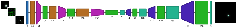
Figure 1: Figure showing the schematic representation of the CAE used in this work. The input image is a compound data cube of $\times$PSF, $\times$iPSFand $\times$iPSF1with dimensions $32\times 32\times 9$ per image. The output image dimensions are $32\times 32\times 3$. The numbers shown indicate the change in dimensions of the image tensor as it propagates through the network. The different components of the network are indicated in the legend. The network diagram was generated using Bäuerle et al. (2021).

The regularization aspect of the network is achieved by using ‘BatchNormalization’ layers in both the encoder and decoder portions. There is much discussion in literature as to whether dropout is necessary for CNNs or whether batch normalization is useful for autoencoders. In this case, based on trial and error we have decided to simply apply ‘BatchNormalization’ layers after each pooling/upsampling layer as might be the case in the final network. The model thus formulated is compiled with the Adam optimizer (Kingma & Ba, 2014) and the loss function BinaryCrossentropy , both from the Keras API. The initial learning rate is $0.0001$ and it decays exponentially at the rate of $0.6$ per $100000$ steps. The model is trained for $350$ epochs with a batch size of $10$. We intend for this method to be a more specific methodological sequel to the work in HW23 in order to provide unbiased shear measurements that do not correlate with the PSF but do so with the truth image. This simple, ‘quick and dirty’ approach does indeed provide results comparable to that of HW23 for specific cases as we will illustrate in the following sections. It is also cheaper in terms of computation time and resources, taking $\sim 3$ hours to train on an NVIDIA GeForce GTX 1650 GPU with 4GB memory and compiled with cuDNN (version 11.4) .

3.3 (Re-)Normalization

A perennial problem in the application of neural networks to astronomical image analysis is the image dynamic range. Dynamic range in astronomical images can vary by many orders of magnitude, while the neural networks require inputs to be of limited dynamic range. The non-linear transformations inside the neural network are typically non-linear over the range $0-1$ and if given an input range that is very different, the system will fundamentally change its properties. The usual procedure is therefore to apply certain normalization factors to the inputs, outputs as well as the truth images. The main issue is that one is “not allowed” to derive these factors from truth images, since for real-life problems we do not have truth images. Instead we argue that the normalization factor should be recalculated with an afterburner maximum likelihood for the amplitude parameter only.

In our case the procedure is as follows:

1. Train the network with input and output images normalized in any sensible manner, e.g. using min-max rescaling to unity interval.

2. When applying to the data, use the same rescaling on the input image as in the training. The output image is now deconvolved, but normalized in an arbitrary manner.

3. Perform a maximum-likelihood fit to the output image normalization. In our case, this involves reconvolving the output image with the PSF and then calculating the renormalization factor as

   $$r=\frac{(\sum_{{\rm pixels}\ i)}{n_{i}p_{i}}}{\sum_{({\rm pixels}\ i)}{p_{i}^{2}}},$$ (2)

   where $p_{i}$ is the output image convolved with PSF and $n$ is the noisy image. This formula can be derived by minimizing the square difference between the $p$ and $n$.

This approach leverages the neural network to do the actual heavy lifting in terms of determining the morphology of the output image, while leveraging the exact solution for the image normalization part. A similar approach can also be used in various deblending approaches employing neural networks, where perhaps multiple component amplitudes can be computed.

Upon implementing this procedure, we have found that the measured fluxes have small negative biases. This is due to the fact that any imperfection in the recovered shape will result in the object amplitude being biased low. To see this, imagine if the image to be fit in amplitude has a source at a completely wrong position. That source would not be able to model the flux of the actual source and therefore its flux would be low (and presumably consistent with the upper limit for the flux of a putative source at the wrong position). In our case, the situation is less dramatic, but sources are still biased low at a few percent. In order to fix this, we model the true total flux $M_{00}$ as a quadratic function in the recovered flux. The motivation for the quadratic function is that we expect morphology to be better recovered with higher fluxes and therefore less biased.

4 Experiments & Results

4.1 Deconvolution performance

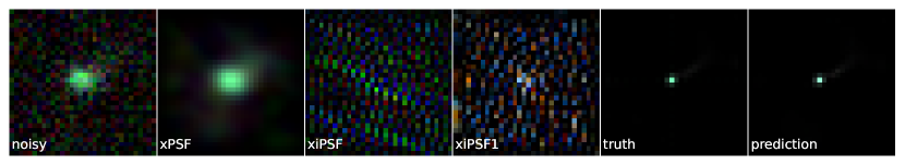
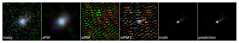
Low SNR

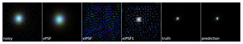
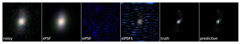
Medium SNR

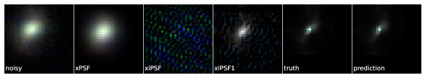
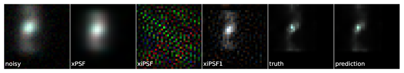
High SNR

Figure 2: Figure showing some typical results from the $\times$PSF-$\times$iPSF-$\times$iPSF1 network. The columns correspond to 1) noisy image, 2) noisy image convolved with the image PSF ($\times$PSF), 3) noisy image convolved with the inverse of the image PSF ($\times$iPSF) 4)noisy image convolved with the image PSF to which a Gaussian filter of standard deviation $1$ is applied ($\times$iPSF1), 5) truth image and 6) the prediction from the network. The rows are arranged according to the SNR as indicated.

We start by conducting experiments with different combinations of the aforementioned $\times$PSF, $\times$iPSFand $\times$iPSF1 data configurations. Some typical results using the data cube $\times$PSF-$\times$iPSF-$\times$iPSF1 are represented in Figure 2. As indicated in the postage stamps, the columns are noisy data, $\times$PSF, $\times$iPSF, $\times$iPSF1, truth and prediction respectively, arranged by the image SNR. We would like to note that these are only the results for the non-blank objects, obtained from a network that was trained with blank images as well.

We see that the network is capable of successfully deconvolving fine structures well below the size of the PSF. The $\times$iPSF1 image is close to a formally regularized solution (e.g. Wiener-filter like). For low SNR objects in Fig 2 it under-regularizes, as indicated by still significant noise features, while for the high SNR it over-regularizes. In any case, the prediction can correctly deconvolve fine structures in the truth image even in the low-noise regime. These images show that as the basic level, the network performs as one would expect. We next turn to more quantitative assessments of its performance.

	$\times$PSF-$\times$iPSF-$\times$iPSF1		$\times$PSF-$\times$iPSF		$\times$iPSF-$\times$iPSF1		$\times$PSF-$\times$iPSF1		$\times$PSF		$\times$iPSF		$\times$iPSF1
	Mean	Median	Mean	Median	Mean	Median	Mean	Median	Mean	Median	Mean	Median	Mean	Median
PSNR	75.177	74.744	73.477	72.873	74.056	73.611	75.378	74.987	74.034	73.709	73.331	72.842	75.290	74.943
1-SSIM	0.0489	0.0177	0.0557	0.0253	0.0507	0.0209	0.0404	0.0165	0.0628	0.0259	0.0708	0.0281	0.0418	0.0173

Table 1: Table showing the differences between the mean and median in the PSNR (dB) and SSIM values for the truth and predicted data sets for the different data cubes. For both PSNR & SSIM, the higher the value, the better the congruence between the truth and the prediction.

In Table 1, we compare the mean and median values of certain standard metrics that are typically used in image analysis for all the data combinations. Peak signal-to-noise ratio (PSNR) is defined as the ratio of maximum possible signal strength to the distorting noise level, expressed in logarithmic decibel scale. It performs a pixel-to-pixel comparison between images, and higher values of this quantity are equated to better quality, and lower values to greater numerical dissimilarities between images (Horé & Ziou 2010). SSIM on the other hand, defines the perceived similarity between images through the correlation of image pixels, thus providing information about contrast, luminance and structure. It maps the structural similarities between two objects, and is often taken as an acceptable proxy to human visual perception, and is as such, considered to be more sensitive to image degradation as a result of compression, noise etc. than PSNR. Here we have used the implementations in scikit-image (Van der Walt et al. 2014) to calculate both PSNR and SSIM. In general, the higher the PSNR and SSIM values are, the better. Here, for SSIM we have opted to show how dissimilar the truth and prediction images are (1-SSIM since the maximum possible value is 1) rather than the values themselves, so the lower the value the better the similarity between the truth and prediction. For both PSNR and SSIM, the best mean and median values is returned by $\times$PSF-$\times$iPSF1, closely followed by the full $\times$PSF-$\times$iPSF-$\times$iPSF1 while $\times$iPSF returns the worst mean and median values.

	$\times$PSF-$\times$iPSF-$\times$iPSF1		$\times$PSF-$\times$iPSF		$\times$iPSF-$\times$iPSF1		$\times$PSF-$\times$iPSF1		$\times$PSF		$\times$iPSF		$\times$iPSF1
	Mean	RMS	Mean	RMS	Mean	RMS	Mean	RMS	Mean	RMS	Mean	RMS	Mean	RMS
$M_{00}$	0.4313	17.6943	0.8253	24.4059	0.6633	24.5903	0.9567	17.9097	-0.5118	26.4617	0.1937	26.2412	0.9077	18.5814
$\left<x\right>$	0.0044	0.6096	0.0293	0.6314	0.0201	0.6543	0.0392	0.5610	0.0237	0.5391	0.0192	0.8376	0.0337	0.6029
$\left<y\right>$	0.0070	0.6034	-0.0166	0.6204	0.0033	0.6282	-0.0070	0.5436	-0.0229	0.5486	0.0365	0.863	0.0144	0.5575
$e_{1}$	-0.0005	0.1443	-0.0050	0.1503	-0.0082	0.1424	-0.0030	0.1376	0.0108	0.1541	-0.0043	0.1585	0.0010	0.1350
$e_{2}$	0.0042	0.1586	-0.0147	0.1719	0.0040	0.1618	-0.0011	0.1561	-0.0117	0.1717	-0.1120	0.1862	-0.0114	0.1605
$\|\boldsymbol{e}\|$	0.0670	0.1425	0.0581	0.1465	0.0486	0.1356	0.0444	0.1308	0.0908	0.1698	0.0729	0.1581	0.0425	0.1281
$s$	-4.3078	11.9458	-2.8706	12.2596	-2.4115	12.2552	-0.3480	9.2682	-8.7653	16.4317	-6.7513	18.1492	-0.8512	9.1547

Table 2: Table showing the mean and RMS values of the differences in moments & other astronomically significant quantities between the true and the predicted images for the different data combinations.

Table 2 shows a comparison of quantities that are physically significant in astronomical image processing in terms of image moments (see Equation 10 in HW23). We have tried to quantify our results in terms of the four major image aspects, i.e., (1) position, (2) flux, (3) shape and (4) size. Here, the central moment $M_{00}$ is a measure of the total flux, $<x>$ & $<y>$ astrometric co-ordinates ($M_{10}$ and $M_{01}$ moments), the second central moments $x^{2}$, & $y^{2}$ ($\mu_{20}$ and $\mu_{02}$) representing size, $s=x^{2}+y^{2}$, and $e_{1}$ & $e_{2}$ the $+$ and $-$ components of ellipticity, and $\|\boldsymbol{e}\|=e_{1}^{2}+e_{2}^{2}$. Since these are the differences between the mean and RMS values of the truth and prediction, the objective is that the absolute value of the difference be as small as possible.

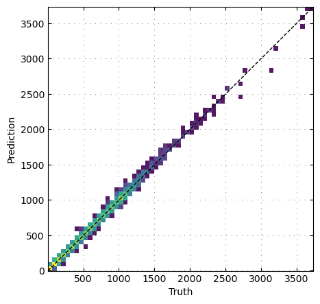
Figure 3: 2-D histogram showing the $M_{00}$ moments of the raw truth data (X-axis) and the re-scaled and flux corrected predictions (Y-axis). We use this to illustrate the accuracy of our re-scaling method and flux corrections.

We apply corrections to the recovered $M_{00}$ values as described in the Section 3.3. The resulting function for the $\times$PSF-$\times$iPSF-$\times$iPSF1 has linear and quadratic coefficients equal to $0.984$ and $2.84\times 10^{-6}$ and a constant term $-1.6$. The error percentage or bias between the predictions and this corrected data are $7.25\%$, $2.15\%$ and $1.5\%$ respectively for the low, medium and high SNR bins and those between the truth data and the corrected predictions are $1.46\%$, $0.22\%$ and $0.066\%$, well within the noise scatter and consistent with no bias.

In Figure 3, we illustrate these results graphically, We plot a 2-d histogram of the $M_{00}$ values for the raw truth data and the prediction values rescaled using the factors calculated in Equation 2 and then flux corrected for the $\times$PSF-$\times$iPSF-$\times$iPSF1 data cube. As can be seen, the $M_{00}$s are within the same range and to a great extent align with each other. We single out the $M_{00}$ moment here to illustrate this effect since all the other quantities that we consider are flux scale independent. Even though only one of the metrics we consider is affected by it, the impact of re-scaling cannot be ignored because $M_{00}$ is representative of the total flux and is therefore quite important in terms of image recovery. We note that all fluxes are biased low. That is because any shape mismatch between the output image and the truth will result in normalization being low.

The best values for both the mean $M_{00}$ (denoting bias) is returned by the $\times$iPSF1 data cube, and the RMS (scatter) by $\times$PSF-$\times$iPSF-$\times$iPSF1, the worst mean by $\times$PSF-$\times$iPSF1, and the worst RMS by $\times$PSF with the other data configurations performing moderately. The best mean value for $\left<x\right>$ is returned by $\times$PSF-$\times$iPSF-$\times$iPSF1 and that for $\left<y\right>$ by $\times$iPSF-$\times$iPSF1. The latter is quite interesting because convolving noisy image with the image PSF ($\times$PSF) is a matched filter for point sources and therefore often used for object detection in astronomical images, but here the object detection aspect seems to be achieved better (albeit marginally) without the $\times$PSF component. It is also worth noting that for mean $\left<y\right>$, $\times$PSF-$\times$iPSF-$\times$iPSF1 and $\times$PSF-$\times$iPSF1 have remarkably similar values while for $\left<x\right>$ the values of $\times$PSF-$\times$iPSF-$\times$iPSF1 is an order of magnitude better than all others. For the RMS value of the astrometric co-ordinates however, $\times$PSF returns the best (lowest) values. All other data cubes exhibit similar performances except for $\times$iPSF which performs the worst.

The best mean value for the $+$ component of ellipticity, $e_{1}$, is returned by $\times$PSF-$\times$iPSF-$\times$iPSF1 and the worst by $\times$PSF; likewise the best RMS value is returned by $\times$iPSF1, closely followed by $\times$PSF-$\times$iPSF1. For the $-$ component of ellipticity, $e_{2}$, the best mean value is returned by $\times$iPSF-$\times$iPSF1 & $\times$PSF-$\times$iPSF-$\times$iPSF1 (the difference between them only 0.0002) and the worst by xiPSF. The latter is a similar result to that of the $\times$PSF being inept at determining object position, because convolution with an inverse PSF ($\times$iPSF) is generally implemented for shape recovery in images. The best RMS value for $e_{2}$ was also returned by $\times$iPSF-$\times$iPSF1 and the worst by both $\times$PSF-$\times$iPSF & $\times$PSF (also 0.0002 difference). For the aggregated ellipticity, $|\boldsymbol{e}\|$, the best mean and RMS values are returned by $\times$iPSF1 and the worst of both by $\times$PSF. For the quantity $s$, denoting the sizes, the best mean value is returned by $\times$PSF-$\times$iPSF, the best RMS by $\times$iPSF1, the worst mean by $\times$PSF and the worst RMS by $\times$iPSF.

In Figure 4, we explore the output ellipticity correlations with PSF & truth image using Equations (29) and (30) in HW23 (Eqs. 29 & 30 hereafter). The left panel denotes the PSF correlation of the predicted and the truth data sets for the different experiments that we have conducted. For an ideal deconvolution, this correlation should be zero.

This is an important quantity since in applications like shear estimation, presence of residual PSF dependence could lead to ‘additive bias’ where shapes are contaminated by PSF (see Mandelbaum 2018 and references therein). An ideal network should remove all PSF dependence in the predicted image, leaving the quantity defined in Eq. 29, $\xi_{PSF}=0$. In order to verify this, we also examined the recovered shapes of objects in relation with the truth image as defined in Eq. 30. For an ideal case this quantity, $\xi_{true}=1$ and this is represented in the right panel of the figure. The different data configurations used as input to the network are denoted in the legend. As is evident from the left panel of the figure, it seems that just $\times$PSF and $\times$PSF-$\times$iPSF both do not seem to provide sufficient and information for the network to remove the residual PSF dependence. All the other combinations seem to be comparable in this respect. We expect the $\times$PSF case to be the worst since the information is simply not present and we indeed find this to be the case. The  & $\times$PSF-$\times$iPSFalso does quite bad, likely by being dominated by the information present in the $\times$PSF. All the data combinations have similar performance with regard to ellipticity recovery as can be seen from the right panel of Figure 4 with marginally better performances by $\times$PSF-$\times$iPSF1 in the low SNR bin, and $\times$iPSF1 in the medium and high SNR bins. For convenience of visualization, the points are slightly offset on the X-axis.

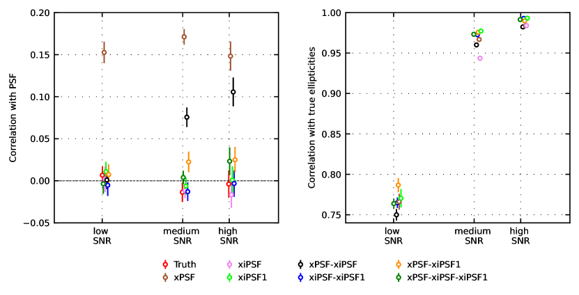
Figure 4: Plot showing the residual PSF dependence (left) and correlation with the truth data (right), separated by SNR. The different data combinations are indicated in the legend below, and they are slightly offset in the X-axis for better visualization.

4.2 Object detection efficiency

Figure 5 shows the confusion matrices for a few selected networks, starting with $\times$PSF  (our worst performing network) to the complete $\times$PSF-$\times$iPSF-$\times$iPSF1 network. Confusion matrices are a standard representation method for the results of machine learning algorithms, especially classification problems. In a typical $2\times 2$ confusion matrix used for binary classification problems, the values represented are the true positive rate (TPR; predictions and truth correspond), false positive rate (FPR; predictions classify as positive while the truth disagrees) from left to right in the first row; the false negative rate (FNR; predictions classify as negative while the truth disagrees) and the true negative rate (TNR; predictions and truth agree that it’s negative) from left to right in the second row. The left diagonal represents the correct classifications. In our case, we can divide our data set into four classes – blanks, low SNR, medium SNR and high SNR. In reconstruction problems such as ours, a threshold needs to be defined to classify the predictions into detections or non-detections. We defined these thresholds upon visual inspection of the histogram representations of the SNRs of the flux corrected predictions.

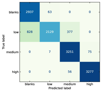
(a) $\times$PSF

(b) $\times$iPSF1

(c) $\times$PSF-$\times$iPSF

(d) $\times$PSF-$\times$iPSF-$\times$iPSF1

Figure 5: Figure showing the confusion matrices for a few selected networks. The true labels are on the Y-axis and the predicted labels on the X-axis.

Part (a) of Figure 5 represents the confusion matrix for the network trained solely using $\times$PSF. For the blanks bin, this network seems to return the best results, which makes sense intuitively, since noisy images are often convolved with their respective PSFs for object detection, and when there is no object, this must make the task easier. However, this reasoning breaks down at the threshold between the blank and low bins for this network and between low and medium bins for this network. The blank vs low confusion seems to be prevalent in the case of all the different networks with varying degrees, it seems especially worse in the case of $\times$PSF. The network trained with $\times$PSF-$\times$iPSF(part (c) seems to perform the best in this respect with an accuracy of $77\%$. The differentiation between the low and the medium bins seems to improve with addition of more/slightly diverse information, as can be seen with the other networks – $\times$iPSF1 in particular seems to deal with this better. The best performance in the medium bin is returned by $\times$iPSF1(part (b)), with an accuracy of $\sim 99\%$. The other networks also return comparable performance TPRs in this bin, indicating an expected trend of the accuracy improving and stabilising as the SNR increases. Part (c) of the figure shows the results from the network trained on $\times$PSF-$\times$iPSF-$\times$iPSF1, and it returns the a marginally high accuracy compared to the other networks in the high SNR bin, $\sim 99\%$.

From both Figure 5 and from Tables 1–2 we can comfortably conclude that the inclusion of $\times$iPSF1, while unconventional, is definitely helpful in both detection and shape recovery, especially in the low SNR regime. It is also similarly evident that only $\times$PSF or only $\times$iPSF is simply not sufficient information for this purpose. As can be seen from Figure 2, even visually it appears that $\times$iPSF1 encompasses salient features of both $\times$PSF and $\times$iPSF, which could be the reason why it is more suited to the purpose at hand. It is also possible that this is data dependent – while we have tried to make our data set as varied as possible, this method might perform differently in a distinct data set, requiring certain adjustments, for e.g. the Gaussian regularising filter might have a different FWHM. The size of the data cube is not linearly related to the running time required, either way the network takes between 2 and 3 hours to complete, which provides a solid scope for experimentation with the data manipulation parameters.

5 Summary & arbitrary conclusions

We present in this work, a simpler approach to remove residual PSF dependence and ellipticity recovery as a follow-up to the work done in HW23. The network implemented in this work is a convolutional autoencoder with 3 encoder and correspondingly 3 decoder layers with respective filter sizes of 64, 128 and 256. $5\times 5$ kernels are used in the convolutional layers (both encoder and decoder) while $2\times 2$ kernels are used in the pooling layers in the encoder and upsampling layers in the decoder. All convolutional layers are activated with the LeakyReLu function and the final output layer with a softplus function. The model is compiled with the Adam optimiser and the loss function used is BinaryCrossentropy. We trained this network with several data configurations, namely, $\times$PSF, $\times$iPSF, $\times$iPSF1 and combinations thereof, results of which are detailed in the preceding sections.

We quantify our results using different metrics, which are displayed in Figures 2 - 5 and Tables 1 - 2. In Figure 2, we show some typical results that is output by the network that is trained with a $\times$PSF-$\times$iPSF-$\times$iPSF1 data cube/combination as a proof of concept. We analyse this further with specific correlations between the predicted data and the PSF and between the predicted data and the true ellipticities in Figure 4 in the three SNR bins. In Tables 1 and 2, we compare significant quantities, both from image analysis and astronomical perspectives to quantify the similarities between the predictions and the truth data. In Table 1, the quantities compared are PSNR and SSIM which are popular metrics used to evaluate image reconstruction. While PSNR and SSIM provide some insight into image recovery from an image analysis standpoint, we are more interested in the recovery of astronomically significant features. To this end, in Table 2, we compare the differences between moment proxies for total fluxes, first order and second order moments averaged over the three bands for the different data combinations. Then we analysed our results using confusion matrices, a very popular form of representation generally used in classification problems by defining thresholds based on SNR, as shown in Figure 5.

We conclude that as is general convention, just convolving the noisy image with the PSF ($\times$PSF) or with the inverse PSF ($\times$iPSF) by themselves are not informative enough for the autoencoder network to efficiently locate the object and remove the PSF dependence. $\times$iPSF1 on the other hand, provides very good results, both by itself and when used in combination with $\times$PSF  or $\times$iPSF1 (or both).

It is hard to declare a clear winner. $\times$iPSF1 is the most economical and is close to the best, although on certain tests, augmenting it with the other two combinations improves results. The simplest interpretation is that $\times$iPSF1 provides a blurry image that is standardized across various observed PSFs – the role of the network is then to simply sharpen and denoise it based on how galaxies in the training set look like. As in any denoising / deblurring approach, the missing information is filled-in based on priors and therefore one should be cautious not to over-interpret galaxy morphologies derived this way.

The main advantages that we see for this method that we have put forth are, (1) simple neural network (2) fast processing, (3) minimal data manipulation and (4) minimal reliance on data features that might not be readily available (e.g. normalization factors). We would also like to emphasize that this method is not a ‘be all and end all’ product in removing PSF dependence and ellipticity recovery by any means. This is merely a simpler way to obtain fast results in this respect using marginal data manipulation. It is possible that its performance will vary in a different data set. While we haven’t tested it on other data sets, we feel that it is not suitable for transfer learning purposes. Although that requirement might be rendered moot by the fact that this is a very fast method even on a data set that contains some 100,000 objects, so training on a similar sized data set would also be a fast process. Our only claim is that for similar data that has both noise and contains one centred object, this is an effective, albeit crude, specific method to obtain denoised data that has excellent correlation to the truth image. There are certain approaches that might be applied to refine this method further. For example, it might be interesting to replace the CAE with a VAE – which would add both some probabilistic and Bayesian aspects to the denoising process. Moreover, VAEs also provide more tuneable parameters that give more control over the latent representation of the input data.

References

- Abbott et al. (2018) Abbott T. M. C., et al., 2018, Phys. Rev. D, 98, 043526
- Arcelin et al. (2021) Arcelin B., Doux C., Aubourg E., Roucelle C., LSST Dark Energy Science Collaboration 2021, MNRAS, 500, 531
- Bertin & Arnouts (1996) Bertin E., Arnouts S., 1996, Astronomy and astrophysics supplement series, 117, 393
- Boucaud et al. (2020) Boucaud A., et al., 2020, Monthly Notices of the Royal Astronomical Society, 491, 2481
- Bäuerle et al. (2021) Bäuerle A., van Onzenoodt C., Ropinski T., 2021, IEEE Transactions on Visualization and Computer Graphics, 27, 2980
- Gardner et al. (2006) Gardner J. P., et al., 2006, Space Sci. Rev., 123, 485
- Glorot et al. (2011) Glorot X., Bordes A., Bengio Y., 2011, in Proceedings of the fourteenth international conference on artificial intelligence and statistics. pp 315–323
- Green et al. (2012) Green J., et al., 2012, arXiv e-prints, p. arXiv:1208.4012
- Hikage et al. (2019) Hikage C., et al., 2019, PASJ, 71, 43
- Horé & Ziou (2010) Horé A., Ziou D., 2010, in 2010 20th International Conference on Pattern Recognition. pp 2366–2369, doi:10.1109/ICPR.2010.579
- Hotelling (1933) Hotelling H., 1933, Journal of educational psychology, 24, 417
- Kingma & Ba (2014) Kingma D. P., Ba J., 2014, arXiv preprint arXiv:1412.6980
- Kingma & Welling (2013) Kingma D. P., Welling M., 2013, arXiv preprint arXiv:1312.6114
- Koekemoer et al. (2007) Koekemoer A. M., et al., 2007, The Astrophysical Journal Supplement Series, 172, 196
- LSST Science Collaboration et al. (2009) LSST Science Collaboration et al., 2009, arXiv e-prints, p. arXiv:0912.0201
- Lanusse et al. (2021) Lanusse F., Mandelbaum R., Ravanbakhsh S., Li C.-L., Freeman P., Póczos B., 2021, Monthly Notices of the Royal Astronomical Society, 504, 5543
- Maas et al. (2013) Maas A. L., Hannun A. Y., Ng A. Y., et al., 2013, in Proc. icml. p. 3
- Mandelbaum (2018) Mandelbaum R., 2018, ARA&A, 56, 393
- Nair & Hinton (2010) Nair V., Hinton G. E., 2010, in Proceedings of the 27th international conference on machine learning (ICML-10). pp 807–814
- Pearson (1901) Pearson K., 1901, The London, Edinburgh, and Dublin Philosophical Magazine and Journal of Science, 6, 559
- Refregier et al. (2010) Refregier A., Amara A., Kitching T. D., Rassat A., Scaramella R., Weller J., 2010, arXiv e-prints, p. arXiv:1001.0061
- Reiman & Göhre (2019) Reiman D. M., Göhre B. E., 2019, Monthly Notices of the Royal Astronomical Society, 485
- Ronneberger et al. (2015) Ronneberger O., Fischer P., Brox T., 2015, arXiv e-prints, p. arXiv:1505.04597
- Rowe et al. (2015) Rowe B., et al., 2015, Astronomy and Computing, 10, 121
- Rumelhart et al. (1985) Rumelhart D. E., Hinton G. E., Williams R. J., et al., 1985, Learning internal representations by error propagation
- Scoville et al. (2007) Scoville N., et al., 2007, The Astrophysical Journal Supplement Series, 172, 38
- Van der Walt et al. (2014) Van der Walt S., Schönberger J. L., Nunez-Iglesias J., Boulogne F., Warner J. D., Yager N., Gouillart E., Yu T., 2014, PeerJ, 2, e453
- Wang et al. (2022) Wang H., Sreejith S., Slosar A. c. v., Lin Y., Yoo S., 2022, Phys. Rev. D, 106, 063023
- Wang et al. (2023) Wang H., Sreejith S., Lin Y., Ramachandra N., Solsar A., Yoo S., 2023, The Open Journal of Astrophysics, 6, 30