Non-parametric regression for robot learning on manifolds

López-Custodio, P.C.1, Bharath, K.2, Kucukyilmaz, A.1, Preston, S.P.2
 
Corresponding author. 1School of Computer Science, University of Nottingham 2School of Mathematical Sciences, University of Nottingham
{pablo.lopez-custodio, karthik.bharath, ayse.kucukyilmaz, simon.preston}@nottingham.ac.uk
Abstract

Many of the tools available for robot learning were designed for Euclidean data. However, many applications in robotics involve manifold-valued data. A common example is orientation; this can be represented as a 3-by-3 rotation matrix or a quaternion, the spaces of which are non-Euclidean manifolds. In robot learning, manifold-valued data are often handled by relating the manifold to a suitable Euclidean space, either by embedding the manifold or by projecting the data onto one or several tangent spaces. These approaches can result in poor predictive accuracy, and convoluted algorithms. In this paper, we propose an “intrinsic” approach to regression that works directly within the manifold. It involves taking a suitable probability distribution on the manifold, letting its parameter be a function of a predictor variable, such as time, then estimating that function non-parametrically via a “local likelihood” method that incorporates a kernel. We name the method kernelised likelihood estimation. The approach is conceptually simple, and generally applicable to different manifolds. We implement it with three different types of manifold-valued data that commonly appear in robotics applications. The results of these experiments show better predictive accuracy than projection-based algorithms.

I Introduction

In recent years, learning from demonstration (LfD) has become an essential approach in robotics research. LfD has been particularly useful for imitating complex human motion which is difficult to mimic by trajectory planning algorithms. Instead, in LfD, the user teaches the robot to follow a trajectory by means of a series of demonstrations.

In this context, Dynamic Movement Primitives (DMP) [1] were introduced to learn a linear attractor system that follows a demonstration. However, in many applications, it is also desired to learn a probability distribution from a series of demonstrations. Encoding how “important” a point is, due to the variability of the demonstrations around it, is crucial in optimal control [2]. This sense of variability can also be exploited to regulate the stiffness of the robot when it interacts with humans [3], to avoid new obstacles [4], or to detect intentions in shared control [5]. Hence, probabilistic approaches have been proposed including Gaussian Mixture Regression (GMR) [6, 7], Probabilistic Movement Primitives (ProMP) [8], and Kernalised Movement Primitives (KMP) [9].

All these LfD methods rely on the multivariate normal distribution as the probabilistic model, and thus only work with Euclidean data. This is not a problem when working in joint space. However, in many applications, working in task space is more convenient. Working in task space aids awareness of the environment, facilitating obstacle avoidance and adaptation to changes. Working in task space is also convenient when learning human skills as it is possible to track objects or parts of the human body. Then these trajectories are transferable to different robots, whilst in joint-space learning, they are exclusive to the robot used for the demonstrations.

However, the problem of not being able to represent orientations in Euclidean space poses a big challenge since the above-mentioned LfD methods are no longer suitable for the training data. A tempting fix is to work with Euler angles. However, since these are three directions, rather than three real numbers, the search space is 𝕋3superscript𝕋3\mathbb{T}^{3}, which is still non-Euclidean. Even worse, the gimbal-lock singularity means an infinity of triads can represent the same orientation which is a major problem for a probabilistic treatment.

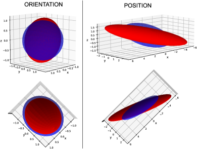
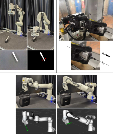
Unfortunately, orientations in task space are not the only type of non-Euclidean data encountered in robotics applications. Any data assuming values in a set where Euclidean geometry of vector spaces is not available is said to be non-Euclidean, and in robotic applications the set can usually be modelled as a smooth manifold. Other examples of manifold-valued data in robotics include: the direction of a table-top grasp (Fig. 1 top-left), the direction of a cutting tool as end-effector (Fig. 1 top-right), the line defining a pointing action, the stiffness matrix of the robot, and the force and velocity manipulability ellipsoids (Fig. 1 bottom).
Refer to caption
Figure 1: Examples of manifold-valued data in robotics. TOP-LEFT: A top-table grasp is an element of 3×𝒮1superscript3superscript𝒮1\mathbb{R}^{3}\times\mathcal{S}^{1} which in this case parametrises the Schoenflies group of displacements, X(4). TOP-RIGHT: The orientation of the cutting tool of the 5-DOF Exechon XMini robot [10] is a direction in 𝒮2superscript𝒮2\mathcal{S}^{2}. BOTTOM: The 7-DOF Franka Panda robot lifts a box in two different configurations but the same pose of end-effector. The direction of maximum force achievable is shown for each configuration. This direction is found by computation of the manipulability ellipsoid, an element of the manifold of SPD matrices, Sym+(6)superscriptSym6\mathrm{Sym}^{+}(6)

A common way to tackle the problem of working with manifold-valued data is through an embedding. Take for example data {𝐱i}i=1Nsuperscriptsubscriptsubscript𝐱𝑖𝑖1𝑁\{\mathbf{x}_{i}\}_{i=1}^{N}, where 𝐱isubscript𝐱𝑖\mathbf{x}_{i} are unit quaternions, so, per notation of Sec.  II-A, 𝐱i𝒮3/2subscript𝐱𝑖superscript𝒮3subscript2\mathbf{x}_{i}\in\mathcal{S}^{3}/\mathbb{Z}_{2}. If a “mean orientation” is of interest, the data is treated as Euclidean and the familiar arithmetic mean N1i𝐱isuperscript𝑁1subscript𝑖subscript𝐱𝑖N^{-1}\sum_{i}\mathbf{x}_{i} is evaluated. This results in a value in 4superscript4\mathbb{R}^{4} that is not a unit quaternion. This can be remedied by renormalising, since i𝐱i/i𝐱isubscript𝑖subscript𝐱𝑖normsubscript𝑖subscript𝐱𝑖\sum_{i}\mathbf{x}_{i}/\|\sum_{i}\mathbf{x}_{i}\| is a “mean” that is indeed in the manifold. This is a simple example of what is sometimes called an extrinsic, or embedding, approach that embeds the manifold into a higher-dimensional Euclidean space, exploits the linear structure of that embedding space, then employs a projection mapping back into the manifold [3]. Extrinsic approaches such as this can work well, especially when the goal is to compute a point-wise quantity such as a mean, but for general manifolds there is not always a natural choice of embedding, nor way to characterise dispersion, and in some settings—such as when the data are highly dispersed on the manifold—estimators can behave erratically.

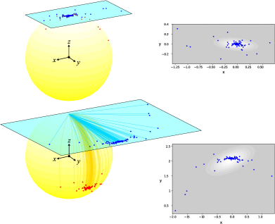
A different approach to analyse manifold-valued data is to employ tangent space projections. This involves picking a point on the manifold, known as the base, and using the inverse exponential map to project the data from the manifold to the tangent plane of the base, which is a Euclidean space where standard tools can then be used. Adequacy of the approach depends on two inter-related considerations: dispersion in the data around the base, and curvature of the manifold. Linearising the data through tangent space projections works well when dispersion is small and curvature of the manifold does not appreciably distort distances of points far from the base; when dispersion is large, the approach is suitable only when curvature of the manifold is non-positive everywhere. Large dispersion will result in distorted estimation of the dispersion structure of the projected data points on the tangent space of the base. To see this, consider the top of Fig. 2 which shows a data set on the unit sphere, 𝒮2superscript𝒮2\mathcal{S}^{2}. This data has been simulated from a distribution with mean 𝛍=(0,0,1)𝛍001\bm{\upmu}=(0,0,1). Using the inverse exponential map, the data is projected onto a tangent plane at 𝛍𝛍\bm{\upmu}, and a normal distribution is fitted there. The obtained covariance matrix has eigenvalues (0.0506,0.004)0.05060.004(0.0506,0.004). Now we rotate the data so they are further away from the tangent point (mimicking data from some “extreme” part of a set of trajectories) as shown at the bottom part of Fig. 2. The data is projected onto the same tangent space as before and a new normal distribution is fitted. The new eigenvalues are (0.198,0.0354)0.1980.0354(0.198,0.0354), significantly larger than before and with different proportion.

Positively curved manifolds cannot be linearised through a single tangent space, and projections using the inverse exponential map are only locally well-defined. An important positively curved manifold that arises in robotics is the quotient manifold 𝒮3/2superscript𝒮3subscript2\mathcal{S}^{3}/\mathbb{Z}_{2} of orientations used to represent three-dimensional rotations as quaternions with antipodal symmetry, where 𝐱𝒮3𝐱superscript𝒮3\mathbf{x}\in\mathcal{S}^{3} and 𝐱𝒮3𝐱superscript𝒮3-\mathbf{x}\in\mathcal{S}^{3} represent the same rotation.

Relatedly, the Riemannian Gaussian distribution [11, 12] is commonly used in probabilistic modelling of manifold-valued data. The distribution is the image under the exponential map of a Gaussian distribution defined on the tangent space of a chosen base point, and operationally amounts to fitting a multivariate normal distribution to data projected onto the tangent space of the base point. Again, curvature of the manifold plays an important role in its definition: for positively curved manifolds, support of the Gaussian distribution on the tangent space is restricted to a suitable subset, while no restrictions are required for non-positively curved manifolds. These distributions have been profitably used for manifold-valued data in robotics [13, 14, 15, 16, 17, 18, 19, 20].

The above-mentioned issues for tangent space projections are exacerbated for data from trajectories on manifolds, since trajectories typically span larger subsets of the manifold, especially when considering one single tangent space [13, 14]. In these cases, curvature effects become more pronounced, and data analysis based on tangent space projections can lead to unreliable conclusions. Notwithstanding these issues, adaptation of trajectory learning methods to manifold-valued data has been done relying on tangent-space projections111The adaptation of DMP to orientations [21, 22, 23] does not require tangent-space projections since it does not provide a probabilistic model.. These include the adaptations of ProMP [24] and KMP [13] to orientational data, and GMR to general Riemannian manifolds [15, 17]
Refer to caption
Figure 2: TOP: a dataset (red) on the unit sphere, 𝒮2superscript𝒮2\mathcal{S}^{2}, and its projection (blue) onto a tangent plane at (0,0,1)001(0,0,1) where the data are centred. BOTTOM: the same data rotated 2π/32𝜋3-2\pi/3 about x𝑥x so they are more distant from (0,0,1)001(0,0,1). These data projected onto the same tangent plane at (0,0,1)001(0,0,1) show how the dispersion structure and hence fitted normal distribution become distorted.

Due to the problems arising from data projection, in this paper we present an alternative method for robot learning that works directly on the manifold. Hence, we say that our method is intrinsic. Our approach exploits the idea of non-parametric regression, which remains largely unexplored in on-manifold robot learning research. In addition, we build upon probability distribution models that are rarely or never used in the robotics field. For example, we make use of the Angular Central Gaussian (ACG) distribution for axial data as a less computationally expensive alternative to the Bingham distribution [25, 26], whose computational complexity makes it unappealing for robotics applications, although it has been used in the pose estimation problem [27] and in reinforcement learning [28]. Our approach is based on the idea of local likelihood [29, 30], where regression is done by incorporating kernel weights into the terms of a log-likelihood expression. By this means, we are able to incorporate probability distributions tailored to the data structure in a regression model that relates a predictor variable to a manifold-valued response. We call our approach kernelised likelihood estimation.

The advantages of our approach are the following:

  • The algorithm is simple. The steps can be summarised in a maximization of a weighted sum of terms. This contrasts with other methods whose complexity stems from the adaptation of Euclidean-designed algorithms to manifold-valued data.

  • As it will be shown in the experiments section, by working intrinsically on the manifold, the estimation is more precise compared to methods that work on the tangent bundle.

  • The intrinsic nature of the estimation method ensures that it can be used for data on both positively and nonpositively curved manifolds.

  • Both trajectory learning and regression can be carried out with the same algorithm.

  • No joint distributions between predictor (input) and response (output) are defined. The shape of the covariance of these joint distributions is affected if either predictor or response are re-scaled, for example, due to a change of units.

  • The predictor is not limited to scalars, it can also be manifold-valued.

  • In the case of trajectory learning, adaptation to via-points (both at the end and in the middle of the trajectory) is simple.

  • A method for generating random trajectories from the learnt model is presented. This method reuses the same idea of kernelised likelihood.

  • Unlike parametric models in which the model complexity is constrained by the parametrisation, the approach we propose incorporates non-parametric estimation, allowing the model to get more flexible as the amount of training data grows.

Model flexibility comes at the cost of new predictions having to depend directly on the training data (rather than some low-dimensional parameter vector); this is a potential disadvantage, though one shared by any non-parametric method.

In this paper, it is assumed that a task-space controller is available. Therefore, we only focus on the learning and generation of trajectories but not on the design of controllers.

This paper is organised as follows: Section II provides an overview of common manifold-valued data in robotics. Section III defines the problem statement to be tackled in this paper. Section IV introduces the method we propose to solve this problem. In this method, a suitable probability distribution model is needed, hence, Section V presents several previously introduced models for different types of manifold-valued data. The proposed method is then tested in a series of experiments presented in Section VI. Finally, conclusions are drawn in Section VII.

The related source code will be made public upon acceptance of the paper.

II Common examples of manifold-valued data in robotics

Manifold-valued data appears in a multitude of applications in robotics. A list of these manifolds is summarised by [31]. Although the method presented in this paper works for any of those manifolds, we focus on the ones introduced in this Section, as these are some of the most commonly encountered manifolds in robotics applications.

II-A Directions, 𝒮d1superscript𝒮𝑑1\mathcal{S}^{d-1}

Directions lie on the unit sphere 𝒮d1:={𝐱|𝐱𝐱=1,𝐱d}assignsuperscript𝒮𝑑1conditional-set𝐱formulae-sequencesuperscript𝐱top𝐱1𝐱superscript𝑑\mathcal{S}^{d-1}:=\{\mathbf{x}\,|\,\mathbf{x}^{\top}\mathbf{x}=1,\,\mathbf{x}\in\mathbb{R}^{d}\}. An example of directional data is the orientation of a rotating cutting tool (Fig. 1, top-right), which is an element of 𝒮2superscript𝒮2\mathcal{S}^{2}. Similarly, the orientation of a table-top grasp is an angle in 𝒮1superscript𝒮1\mathcal{S}^{1} (Fig. 1, top-left), while the whole grasp, including position, is in 3×𝒮1superscript3superscript𝒮1\mathbb{R}^{3}\times\mathcal{S}^{1}. Since the angle is always measured about an axis whose direction is constant, grasps belong to the 4-dimensional group of Schoenflies displacements, X(4) [32]. Other examples of data belonging to the X(4) group include the end-effector poses of the Delta and the SCARA robots.

II-B Axes, 𝒮d/2superscript𝒮𝑑subscript2\mathcal{S}^{d}/\mathbb{Z}_{2}

In the manifold of axes, 𝒮d1/2superscript𝒮𝑑1subscript2\mathcal{S}^{d-1}/\mathbb{Z}_{2}, 𝐱𝒮d1𝐱superscript𝒮𝑑1\mathbf{x}\in\mathcal{S}^{d-1} and its antipodal direction 𝐱𝐱-\mathbf{x} represent the same element. There are plenty of applications involving axial data, but an additional reason that 𝒮d1/2superscript𝒮𝑑1subscript2\mathcal{S}^{d-1}/\mathbb{Z}_{2} is so important is that it is isomorphic to the special orthogonal group, SO(3), defined in the following section. Therefore, methods devised for 𝒮3/2superscript𝒮3subscript2\mathcal{S}^{3}/\mathbb{Z}_{2} can be used directly for applications involving orientational data.

II-C Orientations, the special orthogonal group, SO(3)SO3\mathrm{SO(3)}; and poses, the special Euclidean group, SE(3)SE3\mathrm{SE(3)}

The special orthogonal group of dimension 3, SO(3), is defined as the set of orthogonal matrices of determinant 1. These correspond to rotation matrices in 3-dimensional space. Hence, the orientation of any rigid body can be represented by an element of SO(3).

Consider the map 𝐑:𝒮3SO(3):𝐑superscript𝒮3SO3\mathbf{R}\,:\,\mathcal{S}^{3}\rightarrow\mathrm{SO}(3) defined as:

𝐑(𝐱):=𝐈3+2x1skew(x2,x3,x4)+2skew(x2,x3,x4)2assign𝐑𝐱subscript𝐈32subscript𝑥1skewsubscript𝑥2subscript𝑥3subscript𝑥42skewsuperscriptsubscript𝑥2subscript𝑥3subscript𝑥42\mathbf{R}(\mathbf{x}):=\mathbf{I}_{3}+2x_{1}\,\mathrm{skew}(x_{2},x_{3},x_{4})+2\,\mathrm{skew}(x_{2},x_{3},x_{4})^{2} (1)

where 𝐱:=(x1,x2,x3,x4)𝒮3assign𝐱superscriptsubscript𝑥1subscript𝑥2subscript𝑥3subscript𝑥4topsuperscript𝒮3\mathbf{x}:=(x_{1},x_{2},x_{3},x_{4})^{\top}\in\mathcal{S}^{3}, and

skew(v1,v2,v3):=(0v3v2v30v1v2v10).assignskewsubscript𝑣1subscript𝑣2subscript𝑣30subscript𝑣3subscript𝑣2subscript𝑣30subscript𝑣1subscript𝑣2subscript𝑣10\mathrm{skew}(v_{1},v_{2},v_{3}):=\left(\begin{array}[]{ccc}0&-v_{3}&v_{2}\\ v_{3}&0&-v_{1}\\ -v_{2}&v_{1}&0\\ \end{array}\right).

𝐑()𝐑\mathbf{R}(\cdot) is surjective, however 𝐑(𝐱)=𝐑(𝐱)𝐑𝐱𝐑𝐱\mathbf{R}(\mathbf{x})=\mathbf{R}(-\mathbf{x}), 𝐱𝒮3for-all𝐱superscript𝒮3\forall\mathbf{x}\in\mathcal{S}^{3}. Due to this antipodal redundancy, SO(3) is isomorphic to 𝒮3/2P3superscript𝒮3subscript2𝑃superscript3\mathcal{S}^{3}/\mathbb{Z}_{2}\cong P\mathbb{R}^{3}. In kinematics, (1) provides a map between rotation matrices and unit quaternions.

The Special Euclidean group in 3-dimensional space, SE(3), is the set of rigid-body transformations. It is a Lie group, hence, it allows for a Lie algebra, se(3). SE(3) can be identified with the semidirect product SE(3)=SO(3)3SE3right-normal-factor-semidirect-productSO3superscript3\mathrm{SE}(3)=\mathrm{SO}(3)\rtimes\mathbb{R}^{3}.

The pose (position and orientation) of the end-effector of a robot with respect to a fixed coordinate system is a rigid body transformation and thus an element of SE(3). Therefore, for a task-space trajectory, the data are {(𝐗i,ti)}iNsuperscriptsubscriptsubscript𝐗𝑖subscript𝑡𝑖𝑖𝑁\{(\mathbf{X}_{i},t_{i})\}_{i}^{N}, where 𝐗iSE(3)subscript𝐗𝑖SE3\mathbf{X}_{i}\in\mathrm{SE}(3) is a 4-by-4 transformation matrix, a dual quaternion, or an element of any other parametrisation of SE(3).

For many applications, it is reasonable to work with position and orientation independently. Therefore, the task-space trajectory {(𝐗i,ti)}iNsuperscriptsubscriptsubscript𝐗𝑖subscript𝑡𝑖𝑖𝑁\{(\mathbf{X}_{i},t_{i})\}_{i}^{N} can be represented as {(𝐱i,𝐩i,ti)}iNsuperscriptsubscriptsubscript𝐱𝑖subscript𝐩𝑖subscript𝑡𝑖𝑖𝑁\{(\mathbf{x}_{i},\mathbf{p}_{i},t_{i})\}_{i}^{N}, where 𝐱i𝒮3/2subscript𝐱𝑖superscript𝒮3subscript2\mathbf{x}_{i}\in\mathcal{S}^{3}/\mathbb{Z}_{2} is an orientation, and 𝐩i3subscript𝐩𝑖superscript3\mathbf{p}_{i}\in\mathbb{R}^{3}, a position.

II-D Symmetric positive definite matrices, Sym+(d)superscriptSym𝑑\mathrm{Sym}^{+}(d)

The set of symmetric positive definite (SPD) matrices is defined as Sym+(d):={𝐌Sym(d)|𝐱𝐌𝐱>0𝐱d}assignsuperscriptSym𝑑conditional-set𝐌Sym𝑑superscript𝐱top𝐌𝐱0for-all𝐱superscript𝑑\mathrm{Sym}^{+}(d):=\{\mathbf{M}\in\mathrm{Sym}(d)\,|\,\mathbf{x}^{\top}\mathbf{M}\mathbf{x}>0\,\forall\mathbf{x}\in\mathbb{R}^{d}\}.

Although data in Sym+(d)superscriptSym𝑑\mathrm{Sym}^{+}(d) appear in several robotics applications like stiffness and distance covariance matrices, we now explain one of the most important applications of Sym+(d)superscriptSym𝑑\mathrm{Sym}^{+}(d) in robot arms: the velocity and force manipulability ellipsoids.

Let 𝐪𝕋r𝐪superscript𝕋𝑟\mathbf{q}\in\mathbb{T}^{r} be the vector of joint angles of a robot arm with r𝑟r degrees of freedom (DOF). If the end-effector can move in a d𝑑d-dimensional submanifold of SE(3), then its velocity 𝐯d𝐯superscript𝑑\mathbf{v}\in\mathbb{R}^{d} is related to the joint velocities by 𝐯=𝐉(𝐪)𝐪˙𝐯𝐉𝐪˙𝐪\mathbf{v}=\mathbf{J}(\mathbf{q})\dot{\mathbf{q}}, while the output wrench 𝐟d𝐟superscript𝑑\mathbf{f}\in\mathbb{R}^{d} is related to the joint torques 𝛕r𝛕superscript𝑟\bm{\uptau}\in\mathbb{R}^{r} by 𝛕=𝐉(𝐪)𝐟𝛕superscript𝐉top𝐪𝐟\bm{\uptau}=\mathbf{J}^{\top}(\mathbf{q})\,\mathbf{f}. The matrix 𝐉(𝐪)d×r𝐉𝐪superscript𝑑𝑟\mathbf{J}(\mathbf{q})\in\mathbb{R}^{d\times r} is the Jacobian matrix of the robot at configuration 𝐪𝐪\mathbf{q}.

It is possible to use 𝐉(𝐪)𝐉𝐪\mathbf{J}(\mathbf{q}) to evaluate the performance of the robot at configuration 𝐪𝐪\mathbf{q} [33]. One of such performance indexes evaluates the velocities of the end-effector that can be generated by the set of joint velocities of magnitude one, 𝐪˙𝐪˙=1superscript˙𝐪top˙𝐪1\dot{\mathbf{q}}^{\top}\dot{\mathbf{q}}=1 at 𝐪𝐪\mathbf{q}. If r>d𝑟𝑑r>d, replacing the least-squares solution to 𝐯=𝐉(𝐪)𝐪˙𝐯𝐉𝐪˙𝐪\mathbf{v}=\mathbf{J}(\mathbf{q})\dot{\mathbf{q}}, 𝐪˙=𝐉(𝐪)(𝐉(𝐪)𝐉(𝐪))1𝐯˙𝐪superscript𝐉top𝐪superscript𝐉𝐪superscript𝐉top𝐪1𝐯\dot{\mathbf{q}}=\mathbf{J}^{\top}(\mathbf{q})(\mathbf{J}(\mathbf{q})\mathbf{J}^{\top}(\mathbf{q}))^{-1}\mathbf{v}, in 𝐪˙𝐪˙=1superscript˙𝐪top˙𝐪1\dot{\mathbf{q}}^{\top}\dot{\mathbf{q}}=1 gives:

𝐯(𝐉(𝐪)𝐉(𝐪))1𝐯=1.superscript𝐯topsuperscript𝐉𝐪superscript𝐉top𝐪1𝐯1\mathbf{v}^{\top}\left(\mathbf{J}(\mathbf{q})\mathbf{J}^{\top}(\mathbf{q})\right)^{-1}\mathbf{v}=1. (2)

Define 𝐌(𝐪):=𝐉(𝐪)𝐉(𝐪)Sym+(d)assign𝐌𝐪𝐉𝐪superscript𝐉top𝐪superscriptSym𝑑\mathbf{M}(\mathbf{q}):=\mathbf{J}(\mathbf{q})\mathbf{J}^{\top}(\mathbf{q})\in\mathrm{Sym}^{+}(d), and let {λi}i=1dsuperscriptsubscriptsubscript𝜆𝑖𝑖1𝑑\{\lambda_{i}\}_{i=1}^{d} be its eigenvalues in descending order with corresponding eigenvectors {𝐛i}i=1d𝒮d1superscriptsubscriptsubscript𝐛𝑖𝑖1𝑑superscript𝒮𝑑1\{\mathbf{b}_{i}\}_{i=1}^{d}\subset\mathcal{S}^{d-1}. Then (2) defines an ellipsoid whose axes are parallel to {𝐛i}i=1dsuperscriptsubscriptsubscript𝐛𝑖𝑖1𝑑\{\mathbf{b}_{i}\}_{i=1}^{d} and have lengths {1/λi}i=1dsuperscriptsubscript1subscript𝜆𝑖𝑖1𝑑\{1/\sqrt{\lambda_{i}}\}_{i=1}^{d}. Hence, 𝐯(𝐌(𝐪))1𝐯=1superscript𝐯topsuperscript𝐌𝐪1𝐯1\mathbf{v}^{\top}\left(\mathbf{M}(\mathbf{q})\right)^{-1}\mathbf{v}=1 is known as the velocity manipulability ellipsoid at 𝐪𝐪\mathbf{q}. Equivalently, 𝐟𝐌(𝐪)𝐟=1superscript𝐟top𝐌𝐪𝐟1\mathbf{f}^{\top}\mathbf{M}(\mathbf{q})\mathbf{f}=1 provides a force manipulability ellipsoid.

III Problem statement

In the probabilistic trajectory-learning problem, it is desired to predict a variable (response) for a new input (predictor) given a training dataset representing a series of human demonstrations. It is also required to know the variability of the demonstrations for any value of the predictor. We consider the cases in which either the response or both the response and the predictor lie on a manifold.

In the case of scalar predictor and response in a manifold \mathcal{M}, the training data 𝒟={{(𝐱ij,tij)}j=1Mi}i=1N𝒟superscriptsubscriptsuperscriptsubscriptsubscript𝐱𝑖𝑗subscript𝑡𝑖𝑗𝑗1subscript𝑀𝑖𝑖1𝑁\mathscr{D}=\{\{(\mathbf{x}_{ij},t_{ij})\}_{j=1}^{M_{i}}\}_{i=1}^{N}, 𝐱ij[0,1]subscript𝐱𝑖𝑗01\mathbf{x}_{ij}\in[0,1], 𝐱ijsubscript𝐱𝑖𝑗\mathbf{x}_{ij}\in\mathcal{M}, is a set of N𝑁N trajectories recorded from human demonstrations, each trajectory i𝑖i contains Misubscript𝑀𝑖M_{i} data points. Let P(θ)subscript𝑃𝜃P_{\mathcal{M}}(\theta) be a probability distribution on \mathcal{M} with parameter(s) θ𝜃\theta, so that the mean and dispersion structure are directly or indirectly included in θ𝜃\theta. Then, it is desired to estimate θ^(t)^𝜃𝑡\hat{\theta}(t), for any t[0,1]𝑡01t\in[0,1]. So, we can obtain a trajectory of L𝐿L points, {θk,tk}k=1Lsuperscriptsubscriptsubscript𝜃𝑘subscript𝑡𝑘𝑘1𝐿\{\theta_{k},t_{k}\}_{k=1}^{L}, θk:=θ^(tk)assignsubscript𝜃𝑘^𝜃subscript𝑡𝑘\theta_{k}:=\hat{\theta}(t_{k}).

It is also desired to solve the problem of simple regression. In this case, given a new value of the predictor, the value of the response is estimated based on a training dataset. Hence, the training data set is 𝒟={(𝐱i,𝐭i)}i=1N𝒟superscriptsubscriptsubscript𝐱𝑖subscript𝐭𝑖𝑖1𝑁\mathscr{D}=\{(\mathbf{x}_{i},\mathbf{t}_{i})\}_{i=1}^{N}, 𝐱iOsubscript𝐱𝑖subscript𝑂\mathbf{x}_{i}\in\mathcal{M}_{O}, 𝐱iIsubscript𝐱𝑖subscript𝐼\mathbf{x}_{i}\in\mathcal{M}_{I}, where Isubscript𝐼\mathcal{M}_{I} and Osubscript𝑂\mathcal{M}_{O} are the manifolds of the predictor and response, respectively. The goal is now to estimate 𝐱^O^𝐱subscript𝑂\hat{\mathbf{x}}\in\mathcal{M}_{O} for a new 𝐭I𝐭subscript𝐼\mathbf{t}\in\mathcal{M}_{I}.

IV Robot learning via kernelised likelihood estimation

The approach we develop in this paper extends upon the idea of Nadaraya–Watson kernel regression [34, 35], a non-parametric approach that estimates the response variable for a predictor query point as weighted combinations of the training response cases, with weights chosen according to proximity of predictor values. While Nadaraya–Watson regression is appropriate for Euclidean-valued response data, our approach is appropriate for manifold-valued response data and hence to the problems described in Section III. Furthermore, Nadaraya–Watson regression is usually geared towards computing a point estimate, such as a mean, for each value of the predictor, whereas here we are interested too in estimating the dispersion structure.

IV-A Nadaraya-Watson regression in Euclidean space

Consider training data 𝒟={(xi,ti)}i=1N𝒟superscriptsubscriptsubscript𝑥𝑖subscript𝑡𝑖𝑖1𝑁\mathscr{D}=\{(x_{i},t_{i})\}_{i=1}^{N}, xi,tisubscript𝑥𝑖subscript𝑡𝑖x_{i},t_{i}\in\mathbb{R}. The Nadaraya–Watson estimator of the mean response as a function of the predictor is

μ^(t)=i=1N[Kh(tti)i=1NKh(tti)xi],^𝜇𝑡superscriptsubscript𝑖1𝑁delimited-[]subscript𝐾𝑡subscript𝑡𝑖superscriptsubscript𝑖1𝑁subscript𝐾𝑡subscript𝑡𝑖subscript𝑥𝑖\hat{\mu}(t)=\sum_{i=1}^{N}\left[\dfrac{K_{h}(t-t_{i})}{\sum\limits_{i=1}^{N}K_{h}(t-t_{i})}x_{i}\right], (3)

where Kh(t)subscript𝐾𝑡K_{h}(t) is a non-negative-valued kernel function with bandwidth parameter h>00h>0, a maximum at t=0𝑡0t=0, and Kh(t)dtsubscript𝐾𝑡differential-d𝑡\int K_{h}(t)\mathrm{d}t equal to a constant independently of hh. The value of hh sets a trade-off between fitting and smoothness. A commonly used kernel is defined as Kh(t):=exp(t2/2h2)assignsubscript𝐾𝑡expsuperscript𝑡22superscript2K_{h}(t):=\mathrm{exp}(-t^{2}/2h^{2}).

Writing (3)3(\ref{eq:basic}) as

μ^(t)=i=1NWi(t)xi,^𝜇𝑡superscriptsubscript𝑖1𝑁subscript𝑊𝑖𝑡subscript𝑥𝑖\hat{\mu}(t)=\sum_{i=1}^{N}W_{i}(t)\,x_{i}, (4)

emphasises that the estimator is a simple weighted linear combination of the training response data, with the weight

Wi(t):=Kh(tti)i=1NKh(tti).assignsubscript𝑊𝑖𝑡subscript𝐾𝑡subscript𝑡𝑖superscriptsubscript𝑖1𝑁subscript𝐾𝑡subscript𝑡𝑖W_{i}(t):=\dfrac{K_{h}(t-t_{i})}{\sum\limits_{i=1}^{N}K_{h}(t-t_{i})}. (5)

IV-B Kernelised likelihood estimation

The Nadaraya–Watson estimator (4) is appealing because it is intuitive and simple to compute. However, it does not generalise directly to manifold-valued response data, 𝐱isubscript𝐱𝑖\mathbf{x}_{i}\in\mathcal{M}, because weighted combinations of 𝐱isubscript𝐱𝑖\mathbf{x}_{i} do not in general lie in \mathcal{M}. Instead, consider first a probability distribution P(θ)subscript𝑃𝜃P_{\mathcal{M}}(\theta) defined on the manifold \mathcal{M}, with probability density function f(𝐱;θ)𝑓𝐱𝜃f(\mathbf{x};\theta) and parameter(s) θ𝜃\theta, and write

XP(θ).similar-to𝑋subscript𝑃𝜃X\sim P_{\mathcal{M}}(\theta). (6)

Given a sample of data {𝐱i}i=1Nsuperscriptsubscriptsubscript𝐱𝑖𝑖1𝑁\{\mathbf{x}_{i}\}_{i=1}^{N} assumed to be realisations of (6) independent of each other and from tisubscript𝑡𝑖t_{i}, parameter θ𝜃\theta can be estimated from the data by maximum likelihood estimation (MLE). The MLE of θ𝜃\theta is the maximiser of the log-likelihood:

θ^=argmaxθi=1Nlogf(𝐱i;θ).^𝜃subscript𝜃superscriptsubscript𝑖1𝑁𝑓subscript𝐱𝑖𝜃\hat{\theta}=\arg\max_{\theta}\sum_{i=1}^{N}\log f(\mathbf{x}_{i};\,\theta). (7)

In this paper, instead of the data being independent they are of the paired form {(𝐱i,ti)}i=1Nsuperscriptsubscriptsubscript𝐱𝑖subscript𝑡𝑖𝑖1𝑁\{(\mathbf{x}_{i},t_{i})\}_{i=1}^{N}, and the goal is to predict how the response variable 𝐱isubscript𝐱𝑖\mathbf{x}_{i} depends on the predictor tisubscript𝑡𝑖t_{i}. To this end we consider models of the form:

(X|T=t)P(θ(t)).similar-toconditional𝑋𝑇𝑡subscript𝑃𝜃𝑡(X|T=t)\sim P_{\mathcal{M}}(\theta(t)). (8)

This is still somewhat general, because it remains to specify how θ(t)𝜃𝑡\theta(t) depends on t𝑡t. We impose this dependence by prescribing

θ^(t)=argmaxθi=1NWi(t)logf(𝐱i;θ),^𝜃𝑡subscript𝜃superscriptsubscript𝑖1𝑁subscript𝑊𝑖𝑡𝑓subscript𝐱𝑖𝜃\hat{\theta}(t)=\arg\max_{\theta}\sum_{i=1}^{N}W_{i}(t)\log f(\mathbf{x}_{i};\,\theta), (9)

where Wi(t)subscript𝑊𝑖𝑡W_{i}(t) is as defined in (5). This is maximising a “local likelihood” in the sense of [30]. Reflecting how the local likelihood incorporates kernel weights, we call our approach kernelised likelihood estimation (KLE).

Once an estimate θ^(t)^𝜃𝑡\hat{\theta}(t) is computed from training data then, by (8), an estimate of 𝔼(X|T=t)𝔼conditional𝑋𝑇𝑡\mathbb{E}(X|T=t) is

𝛍^(t)=𝔼(P(θ^(t))),^𝛍𝑡𝔼subscript𝑃^𝜃𝑡\hat{\bm{\upmu}}(t)=\mathbb{E}\big{(}P_{\mathcal{M}}\big{(}\hat{\theta}(t)\big{)}\big{)}, (10)

where 𝔼𝔼\mathbb{E} denotes expectation. Thus, 𝛍^(t)^𝛍𝑡\hat{\bm{\upmu}}(t) defines a smooth path through the training data and, in this sense, provides a solution to the on-manifold regression problem.

For the problem of trajectories on manifolds with training data 𝒟={{(𝐱ij,tij)}j=1Mi}i=1N𝒟superscriptsubscriptsuperscriptsubscriptsubscript𝐱𝑖𝑗subscript𝑡𝑖𝑗𝑗1subscript𝑀𝑖𝑖1𝑁\mathscr{D}=\{\{(\mathbf{x}_{ij},t_{ij})\}_{j=1}^{M_{i}}\}_{i=1}^{N}, 𝐱ij[0,1]subscript𝐱𝑖𝑗01\mathbf{x}_{ij}\in[0,1], 𝐱ijsubscript𝐱𝑖𝑗\mathbf{x}_{ij}\in\mathcal{M}, we simply rewrite Eq. (9) as:

θ^(t)=argmaxθi=1Ni=1MiWij(t)logf(𝐱ij;θ),^𝜃𝑡subscript𝜃superscriptsubscript𝑖1𝑁superscriptsubscript𝑖1subscript𝑀𝑖subscript𝑊𝑖𝑗𝑡𝑓subscript𝐱𝑖𝑗𝜃\hat{\theta}(t)=\arg\max_{\theta}\sum_{i=1}^{N}\sum_{i=1}^{M_{i}}W_{ij}(t)\log f(\mathbf{x}_{ij};\,\theta), (11)

where

Wij(t):=Kh(ttij)i=1Nj=1MiKh(ttij).assignsubscript𝑊𝑖𝑗𝑡subscript𝐾𝑡subscript𝑡𝑖𝑗superscriptsubscript𝑖1𝑁superscriptsubscript𝑗1subscript𝑀𝑖subscript𝐾𝑡subscript𝑡𝑖𝑗W_{ij}(t):=\dfrac{K_{h}(t-t_{ij})}{\sum\limits_{i=1}^{N}\sum\limits_{j=1}^{M_{i}}K_{h}(t-t_{ij})}. (12)

To illustrate the application of the KLE method, consider the following scenarios with scalar, Euclidean and manifold-valued data:

Scalar response: Consider the case of xi,tisubscript𝑥𝑖subscript𝑡𝑖x_{i},t_{i}\in\mathbb{R} (that is, let \mathcal{M} be \mathbb{R}), let P(θ)subscript𝑃𝜃P_{\mathcal{M}}(\theta) with θ={μ,σ2}𝜃𝜇superscript𝜎2\theta=\{\mu,\sigma^{2}\} be the normal distribution 𝒩(μ,σ2)𝒩𝜇superscript𝜎2\mathcal{N}(\mu,\sigma^{2}). Then, by Eq. (9), θ^(t)={μ^(t),σ^2(t)}^𝜃𝑡^𝜇𝑡superscript^𝜎2𝑡\hat{\theta}(t)=\{\hat{\mu}(t),\hat{\sigma}^{2}(t)\}, where

μ^(t)=i=1NWi(t)xi,σ^2(t)=i=1NWi(t)[xiμ^(t)]2.formulae-sequence^𝜇𝑡superscriptsubscript𝑖1𝑁subscript𝑊𝑖𝑡subscript𝑥𝑖superscript^𝜎2𝑡superscriptsubscript𝑖1𝑁subscript𝑊𝑖𝑡superscriptdelimited-[]subscript𝑥𝑖^𝜇𝑡2\hat{\mu}(t)=\sum_{i=1}^{N}W_{i}(t)x_{i},\quad\hat{\sigma}^{2}(t)=\sum_{i=1}^{N}W_{i}(t)[x_{i}-\hat{\mu}(t)]^{2}. (13)

Thus in this case the estimator of the mean, μ^(t)^𝜇𝑡\hat{\mu}(t), is exactly the Nadaraya-Watson estimator (4). This approach further provides an estimate of how the variance, σ2superscript𝜎2{\sigma}^{2}, varies with the predictor, t𝑡t.

Euclidean response: Now consider 𝒟={{(𝐱ij,tij)}j=1Mi}i=1N𝒟superscriptsubscriptsuperscriptsubscriptsubscript𝐱𝑖𝑗subscript𝑡𝑖𝑗𝑗1subscript𝑀𝑖𝑖1𝑁\mathscr{D}=\{\{(\mathbf{x}_{ij},t_{ij})\}_{j=1}^{M_{i}}\}_{i=1}^{N}, 𝐱ijdsubscript𝐱𝑖𝑗superscript𝑑\mathbf{x}_{ij}\in\mathbb{R}^{d}, tij[0,1]subscript𝑡𝑖𝑗01t_{ij}\in[0,1] (that is, let \mathcal{M} be dsuperscript𝑑\mathbb{R}^{d}), and let P(θ)subscript𝑃𝜃P_{\mathcal{M}}(\theta) with θ={𝛍,𝚺}𝜃𝛍𝚺\theta=\{\bm{\upmu},{\bm{\Sigma}}\} be the multivariate normal distribution 𝒩(𝛍,𝚺)𝒩𝛍𝚺\mathcal{N}(\bm{\upmu},{\bm{\Sigma}}). Then θ^(t)={𝛍^(t),𝚺^(t)}^𝜃𝑡^𝛍𝑡^𝚺𝑡\hat{\theta}(t)=\{\hat{\bm{\upmu}}(t),\hat{{\bm{\Sigma}}}(t)\}, where

𝛍^(t)=i=1Nj=1MiWij(t)𝐱ij,𝚺^(t)=i=1Nj=1Mi[Wij(t)(𝐱ij𝛍^(t))(𝐱ij𝛍^(t))],formulae-sequence^𝛍𝑡superscriptsubscript𝑖1𝑁superscriptsubscript𝑗1subscript𝑀𝑖subscript𝑊𝑖𝑗𝑡subscript𝐱𝑖𝑗^𝚺𝑡superscriptsubscript𝑖1𝑁superscriptsubscript𝑗1subscript𝑀𝑖delimited-[]subscript𝑊𝑖𝑗𝑡subscript𝐱𝑖𝑗^𝛍𝑡superscriptsubscript𝐱𝑖𝑗^𝛍𝑡top\begin{gathered}\hat{\bm{\upmu}}(t)=\sum_{i=1}^{N}\sum_{j=1}^{M_{i}}W_{ij}(t)\,\mathbf{x}_{ij},\\ \hat{\bm{\Sigma}}(t)=\sum_{i=1}^{N}\sum_{j=1}^{M_{i}}\left[W_{ij}(t)\,\left(\mathbf{x}_{ij}-\hat{\bm{\upmu}}(t)\right)\left(\mathbf{x}_{ij}-\hat{\bm{\upmu}}(t)\right)^{\top}\right],\end{gathered} (14)

where the weights Wij(t)subscript𝑊𝑖𝑗𝑡W_{ij}(t) Eq. (12). The proof of Eq. (14) is given in Appendix A.

Manifold-valued response: To illustrate the application of the KLE method to on-manifold trajectory learning, consider the pseudocode in Algorithm 1. In this case, 𝒟={{(𝐱ij,tij)}j=1Mi}i=1N𝒟superscriptsubscriptsuperscriptsubscriptsubscript𝐱𝑖𝑗subscript𝑡𝑖𝑗𝑗1subscript𝑀𝑖𝑖1𝑁\mathscr{D}=\{\{(\mathbf{x}_{ij},t_{ij})\}_{j=1}^{M_{i}}\}_{i=1}^{N}, 𝐱ij𝒮d1/2subscript𝐱𝑖𝑗superscript𝒮𝑑1subscript2\mathbf{x}_{ij}\in\mathcal{S}^{d-1}/\mathbb{Z}_{2}, tij[0,1]subscript𝑡𝑖𝑗01t_{ij}\in[0,1], that is, \mathcal{M} is 𝒮d1/2superscript𝒮𝑑1subscript2\mathcal{S}^{d-1}/\mathbb{Z}_{2}. To model the data, an ACG distribution (with parameter 𝚲𝚲\bm{\Lambda}) is used. This, and other models of distributions on manifolds, are explained in detail in Section V. In Algorithm 1, the function Ker_MLE_ACG can be replaced by the corresponding solution to the KLE in Eq. (9) for a probability distribution that is suitable for the data. Many models admit a simple solution for Eq. (9). It will be seen in Section V that for the ACG distribution on 𝒮d1/2superscript𝒮𝑑1subscript2\mathcal{S}^{d-1}/\mathbb{Z}_{2}, and for the Lognormal distribution on Sym+(d)superscriptSym𝑑\mathrm{Sym}^{+}(d), such a solution simplifies to Eq. (20), and Eqs. (26) and (27), respectively. However, it will be seen that for the ESAG distribution on 𝒮d1superscript𝒮𝑑1\mathcal{S}^{d-1} no simplified expression is known, and hence, Eq. (9) has to be solved with a numerical method. Finally, for the Euclidean case, Eq. (14) give the solution to the maximization of the kernelised likelihood estimation.

It can be seen that Algorithm 1 has a simpler structure than most of the other methods for on-manifold trajectory learning.

Manifold-valued predictor: In the case of a manifold-valued predictor, 𝐭ijIsubscript𝐭𝑖𝑗subscript𝐼\mathbf{t}_{ij}\in\mathcal{M}_{I}, Eq. (9) holds with a kernel of the form Kh(dI(𝐭,𝐭ij))subscript𝐾subscript𝑑subscript𝐼𝐭subscript𝐭𝑖𝑗K_{h}(d_{\mathcal{M}_{I}}(\mathbf{t},\mathbf{t}_{ij})), where dI()subscript𝑑subscript𝐼d_{\mathcal{M}_{I}}(\cdot) is a metric on Isubscript𝐼\mathcal{M}_{I}.

1 Function Ker_MLE_ACG(t𝑡t, 𝒟𝒟\mathscr{D}, hh, ε𝜀\varepsilon):
2       𝚲^old=𝐈dsubscript^𝚲oldsubscript𝐈𝑑\hat{\bm{\Lambda}}_{\mathrm{old}}=\mathbf{I}_{d}
3       do
4             𝚲^newsubscript^𝚲new\hat{\bm{\Lambda}}_{\mathrm{new}} \leftarrow Eq.(20) // input: t,𝒟,h𝑡𝒟t,\mathscr{D},h
5             E=dSPD(𝚲^old,𝚲^new)𝐸subscript𝑑SPDsubscript^𝚲oldsubscript^𝚲newE=d_{\mathrm{SPD}}(\hat{\bm{\Lambda}}_{\mathrm{old}},\hat{\bm{\Lambda}}_{\mathrm{new}})
6             𝚲^old=𝚲^newsubscript^𝚲oldsubscript^𝚲new\hat{\bm{\Lambda}}_{\mathrm{old}}=\hat{\bm{\Lambda}}_{\mathrm{new}}
7            
8      while E<ε𝐸𝜀E<\varepsilon
9 return 𝚲^newsubscript^𝚲new\hat{\bm{\Lambda}}_{\mathrm{new}}
10
11 Function main(𝒟𝒟\mathscr{D}, T𝑇T, hh, ε𝜀\varepsilon):
12       for n=1𝑛1n=1 to T𝑇T do
13             tn=(n1)/(T1)subscript𝑡𝑛𝑛1𝑇1t_{n}=(n-1)/(T-1)
14             𝚲^n=subscript^𝚲𝑛absent\hat{\bm{\Lambda}}_{n}=\,Ker_MLE_ACG(tn,𝒟,h,ε)subscript𝑡𝑛𝒟𝜀\,(t_{n},\mathscr{D},h,\varepsilon)
15            
16       end for
17      
18 return {tn,𝚲^n}n=1Tsuperscriptsubscriptsubscript𝑡𝑛subscript^𝚲𝑛𝑛1𝑇\{t_{n},\hat{\bm{\Lambda}}_{n}\}_{n=1}^{T}
Algorithm 1 Trajectory learning with ACG distribution

IV-C Trajectory adaptation to via-points, and blending of trajectories

Consider the simplest case of a scalar trajectories dataset 𝒟={{(xij,tij)}j=1Mi}i=1N𝒟superscriptsubscriptsuperscriptsubscriptsubscript𝑥𝑖𝑗subscript𝑡𝑖𝑗𝑗1subscript𝑀𝑖𝑖1𝑁\mathscr{D}=\{\{(x_{ij},t_{ij})\}_{j=1}^{M_{i}}\}_{i=1}^{N}, xijsubscript𝑥𝑖𝑗x_{ij}\in\mathbb{R}, tij[0,1]subscript𝑡𝑖𝑗01t_{ij}\in[0,1]. Then μ^(t)^𝜇𝑡\hat{\mu}(t) and σ^(t)^𝜎𝑡\hat{\sigma}(t), t[0,1]𝑡01t\in[0,1], can be determined by Eq (13). It is desired to adapt this model so that the trajectories pass through μsuperscript𝜇\mu^{*} at tsuperscript𝑡t^{*} with an uncertainty controlled by σsuperscript𝜎\sigma^{*}.

To adapt this model, we synthetically generate a second dataset ={{(yij,tj)}j=1R}i=1Ssuperscriptsubscriptsuperscriptsubscriptsubscript𝑦𝑖𝑗subscript𝑡𝑗𝑗1𝑅𝑖1𝑆\mathscr{E}=\{\{(y_{ij},t_{j})\}_{j=1}^{R}\}_{i=1}^{S}, where for every tjsubscript𝑡𝑗t_{j}, a set {yij}i=1Ssuperscriptsubscriptsubscript𝑦𝑖𝑗𝑖1𝑆\{y_{ij}\}_{i=1}^{S}, yij𝒩(μ,σ)similar-tosubscript𝑦𝑖𝑗𝒩superscript𝜇superscript𝜎y_{ij}\sim\mathcal{N}(\mu^{*},\sigma^{*}), is sampled.

Then, the adapted model is obtained as a mixture of 𝒟𝒟\mathscr{D} and \mathscr{E}. The kernels weighting 𝒟𝒟\mathscr{D} and \mathscr{E} are now multiplied by activation functions α(t)𝛼𝑡\alpha(t) and β(t):=1α(t)assign𝛽𝑡1𝛼𝑡\beta(t):=1-\alpha(t), respectively, so that the contributions of the data points are activated or deactivated in the KLE algorithm. Hence, the adapted mean yields:

μ^(t)^𝜇𝑡\displaystyle\hat{\mu}(t) =\displaystyle= 1C(t)[i=1Nj=1Miα(tij)Kh(ttij)xij\displaystyle\frac{1}{C(t)}\left[\sum\limits_{i=1}^{N}\sum\limits_{j=1}^{M_{i}}\alpha(t_{ij})K_{h}(t-t_{ij})x_{ij}\right.
+i=1Sj=1Rβ(tj)Kh(ttj)yij],\displaystyle\left.+\sum\limits_{i=1}^{S}\sum\limits\limits_{j=1}^{R}\beta(t_{j})K_{h}(t-t_{j})y_{ij}\right],

where

C(t)𝐶𝑡\displaystyle C(t) =\displaystyle= i=1Nj=1Miα(tij)Kh(ttij)superscriptsubscript𝑖1𝑁superscriptsubscript𝑗1subscript𝑀𝑖𝛼subscript𝑡𝑖𝑗subscript𝐾𝑡subscript𝑡𝑖𝑗\displaystyle\sum\limits_{i=1}^{N}\sum\limits_{j=1}^{M_{i}}\alpha(t_{ij})K_{h}(t-t_{ij})
+i=1Sj=1Rβ(tj)Kh(ttj),superscriptsubscript𝑖1𝑆superscriptsubscript𝑗1𝑅𝛽subscript𝑡𝑗subscript𝐾𝑡subscript𝑡𝑗\displaystyle+\sum\limits_{i=1}^{S}\sum\limits\limits_{j=1}^{R}\beta(t_{j})K_{h}(t-t_{j}),

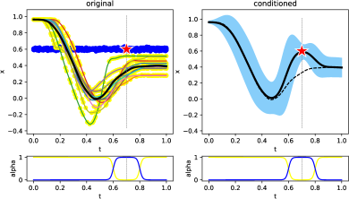
where α(t)0𝛼superscript𝑡0\alpha(t^{*})\approx 0 and β(t)1𝛽superscript𝑡1\beta(t^{*})\approx 1, while α(t)1𝛼𝑡1\alpha(t)\approx 1 and β(t)0𝛽𝑡0\beta(t)\approx 0 for t𝑡t far away from tsuperscript𝑡t^{*}. The adapted σ^(t)^𝜎𝑡\hat{\sigma}(t) is obtained inserting the same activation functions. Fig. 3 shows an example in which a series of scalar demonstrations are adapted to μ=0.6superscript𝜇0.6\mu^{*}=0.6 at t=0.7superscript𝑡0.7t^{*}=0.7.

Refer to caption
Figure 3: Adaptation of scalar trajectories to μ=0.6superscript𝜇0.6\mu^{*}=0.6 at t=0.7superscript𝑡0.7t^{*}=0.7. LEFT: 𝒟𝒟\mathscr{D} (yellow dots) consists of 700 samples taken from 10 demonstrated curves. The resulting μ^(t)^𝜇𝑡\hat{\mu}(t) is shown in thick black curve. \mathscr{E} (blue dots) is generated with μ=0.6superscript𝜇0.6\mu^{*}=0.6 and σ=0.001superscript𝜎0.001\sigma^{*}=0.001. BOTTOM: The activation functions correspond to β(t)=0.5tanh(50(tt+0.1))0.5tanh(50(tt0.1))𝛽𝑡0.550𝑡superscript𝑡0.10.550𝑡superscript𝑡0.1\beta(t)=0.5\tanh(50(t-t^{*}+0.1))-0.5\tanh(50(t-t^{*}-0.1)) and α(t)=1β(t)𝛼𝑡1𝛽𝑡\alpha(t)=1-\beta(t). RIGHT: The result of adaptation with the blue area showing ±1.5σ^(t)plus-or-minus1.5^𝜎𝑡\pm 1.5\hat{\sigma}(t).

Since this modification to the KLE algorithm simply acts on the kernels - by weighting them with the activation functions - the same change is applied to the kernels in Eq (9) in order to adapt trajectories on manifolds to new via-points.

The problem of trajectory blending can be solved by the same method by letting the activation functions act on the data points of the two trajectory sets to be blended. In this case, the activation functions are smoothed step functions.

IV-D Trajectory generation

After θ^(t)^𝜃𝑡\hat{\theta}(t) has been computed for a trajectories dataset 𝒟={{(𝐱ij,tij)}j=1Mi}i=1N𝒟superscriptsubscriptsuperscriptsubscriptsubscript𝐱𝑖𝑗subscript𝑡𝑖𝑗𝑗1subscript𝑀𝑖𝑖1𝑁\mathscr{D}=\{\{(\mathbf{x}_{ij},t_{ij})\}_{j=1}^{M_{i}}\}_{i=1}^{N}, 𝐱ijsubscript𝐱𝑖𝑗\mathbf{x}_{ij}\in\mathcal{M}, tij[0,1]subscript𝑡𝑖𝑗01t_{ij}\in[0,1], new trajectories can be generated around the mean by re-sampling and smoothing along t[0,1]𝑡01t\in[0,1]. First, generate a set 𝒟r={(𝐱r,i,tr,i)}i=1Nrsubscript𝒟𝑟superscriptsubscriptsubscript𝐱𝑟𝑖subscript𝑡𝑟𝑖𝑖1subscript𝑁𝑟\mathscr{D}_{r}=\{(\mathbf{x}_{r,i},t_{r,i})\}_{i=1}^{N_{r}}, where 𝐱r,iP(θ^(tr,i))similar-tosubscript𝐱𝑟𝑖subscript𝑃^𝜃subscript𝑡𝑟𝑖\mathbf{x}_{r,i}\sim P_{\mathcal{M}}(\hat{\theta}(t_{r,i})). Then, apply the KLE regression from Eq. (9) as a smoother for 𝒟rsubscript𝒟𝑟\mathscr{D}_{r}. This results in the estimation of the parameter θ^r(t)subscript^𝜃𝑟𝑡\hat{\theta}_{r}(t) for 𝒟rsubscript𝒟𝑟\mathscr{D}_{r}. Then, the generated curve, 𝛍^r(t)subscript^𝛍𝑟𝑡\hat{\bm{\upmu}}_{r}(t), is defined by Eq. (10), by taking θ^(t)^𝜃𝑡\hat{\theta}(t) equal to θ^r(t)subscript^𝜃𝑟𝑡\hat{\theta}_{r}(t). Consider the special case when \mathcal{M} is dsuperscript𝑑\mathbb{R}^{d}, Psubscript𝑃P_{\mathcal{M}} is the normal distribution, and θ^r(t)subscript^𝜃𝑟𝑡\hat{\theta}_{r}(t) in Eq. (10) is treated as random (depending on the sampling distribution of the training data) then 𝛍^r(t)subscript^𝛍𝑟𝑡\hat{\bm{\upmu}}_{r}(t) is a Gaussian Process (GP). Hence the proposed approach to trajectory generation is a generalization to \mathcal{M} of a GP model in dsuperscript𝑑\mathbb{R}^{d}; see Appendix A for further explanation.

IV-E Autonomous systems

For trajectories in task space, velocities can be learnt as well in order to generate time-independent trajectories. Hence, the training data for an autonomous system is 𝒟={{(𝐓ij,𝐕ij,tij)}j=1Mi}i=1N𝒟superscriptsubscriptsuperscriptsubscriptsubscript𝐓𝑖𝑗subscript𝐕𝑖𝑗subscript𝑡𝑖𝑗𝑗1subscript𝑀𝑖𝑖1𝑁\mathscr{D}=\{\{(\mathbf{T}_{ij},\mathbf{V}_{ij},t_{ij})\}_{j=1}^{M_{i}}\}_{i=1}^{N}, where 𝐓ijSE(3)subscript𝐓𝑖𝑗SE3\mathbf{T}_{ij}\in\mathrm{SE}(3) is a pose and 𝐕ijse(3)subscript𝐕𝑖𝑗se3\mathbf{V}_{ij}\in\mathrm{se}(3) a twist. The proposed on-manifold learning method allows to learn both the position and the orientation parts of 𝐓ijsubscript𝐓𝑖𝑗\mathbf{T}_{ij}, and since se(3) is a vector space, 𝐕ijsubscript𝐕𝑖𝑗\mathbf{V}_{ij} is easy to learn with the same method using the multivariate normal distribution as model (Eq. (14)). Finally, the generated trajectories have the form {(𝐓n,𝐕n)}n=1Tsuperscriptsubscriptsubscript𝐓𝑛subscript𝐕𝑛𝑛1𝑇\{(\mathbf{T}_{n},\mathbf{V}_{n})\}_{n=1}^{T}. Since se(3) enjoys of Euclidean structure, the learning of 𝐕ijsubscript𝐕𝑖𝑗\mathbf{V}_{ij} is not taken into account in the rest of the paper.

V Probability distributions on relevant manifolds

The method described in Section IV requires the use of a probability distribution, 𝒫(θ)subscript𝒫𝜃\mathcal{P}_{\mathcal{M}}(\theta), on the manifold, \mathcal{M}, where the response variable lies. In this section, we introduce probability distributions relevant to the manifolds introduced in Section II. For each distribution, we present the probability density function and the “standard” MLE solution given independent identically distributed data; then we present the new kernelised solution, that is, the solution of (9), that solves the regression problem involving response data on \mathcal{M}.

V-A The elliptically symmetric angular Gaussian distribution on 𝒮d1superscript𝒮𝑑1\mathcal{S}^{d-1}

Given 𝐲𝒩(𝛍,𝐕)similar-to𝐲𝒩𝛍𝐕\mathbf{y}\sim\mathcal{N}(\bm{\upmu},\mathbf{V}), 𝐲d𝐲superscript𝑑\mathbf{y}\in\mathbb{R}^{d}, with constraints 𝐕𝛍=𝛍𝐕𝛍𝛍\mathbf{V}\bm{\upmu}=\bm{\upmu} and |𝐕|=1𝐕1|\mathbf{V}|=1, the directions 𝐱:=𝐲/𝐲𝒮d1assign𝐱𝐲norm𝐲superscript𝒮𝑑1\mathbf{x}:=\mathbf{y}/\|\mathbf{y}\|\in\mathcal{S}^{d-1} have an elliptically symmetric angular Gaussian (ESAG) distribution with density [36]:

fESAG(𝐱;𝛍,𝐕):=Cd(𝐱𝐕1𝐱)d/2exp[12{(𝐱𝛍)2𝐱𝐕1𝐱𝛍𝛍}]Md1(𝐱𝛍(𝐱𝐕1𝐱)1/2),assignsubscript𝑓ESAG𝐱𝛍𝐕subscript𝐶𝑑superscriptsuperscript𝐱topsuperscript𝐕1𝐱𝑑2expdelimited-[]12superscriptsuperscript𝐱top𝛍2superscript𝐱topsuperscript𝐕1𝐱superscript𝛍top𝛍subscript𝑀𝑑1superscript𝐱top𝛍superscriptsuperscript𝐱topsuperscript𝐕1𝐱12\begin{split}f_{\mathrm{ESAG}}(\mathbf{x};\,\bm{\upmu},\,\mathbf{V}):=&\frac{C_{d}}{(\mathbf{x}^{\top}\mathbf{V}^{-1}\mathbf{x})^{d/2}}\mathrm{exp}\Bigg{[}\frac{1}{2}\Bigg{\{}\frac{(\mathbf{x}^{\top}\bm{\upmu})^{2}}{\mathbf{x}^{\top}\mathbf{V}^{-1}\mathbf{x}}\\ &-\bm{\upmu}^{\top}\bm{\upmu}\Bigg{\}}\Bigg{]}M_{d-1}\left(\frac{\mathbf{x}^{\top}\bm{\upmu}}{(\mathbf{x}^{\top}\mathbf{V}^{-1}\mathbf{x})^{1/2}}\right),\end{split} (15)

where Cd:=1/(2π)(d1)/2assignsubscript𝐶𝑑1superscript2𝜋𝑑12C_{d}:=1/(2\pi)^{(d-1)/2} and, for d=2𝑑2d=2 and 3, respectively:

M1(α)subscript𝑀1𝛼\displaystyle M_{1}(\alpha) :=assign\displaystyle:= αΦ(α)+ϕ(α),𝛼Φ𝛼italic-ϕ𝛼\displaystyle\alpha\Phi(\alpha)+\phi(\alpha),
M2(α)subscript𝑀2𝛼\displaystyle M_{2}(\alpha) :=assign\displaystyle:= (1+α2)Φ(α)+αϕ(α),1superscript𝛼2Φ𝛼𝛼italic-ϕ𝛼\displaystyle(1+\alpha^{2})\Phi(\alpha)+\alpha\phi(\alpha),

where ϕ()italic-ϕ\phi(\cdot) and Φ()Φ\Phi(\cdot) are the functions for standard normal probability density and cumulative density, respectively. See [36] for Md1subscript𝑀𝑑1M_{d-1} with d>3𝑑3d>3.

Let 0ρ1,ρd=10\leq\rho_{1},\leq\ldots\leq\rho_{d}=1 be the eigenvalues of 𝐕𝐕\mathbf{V} with corresponding eigenvectors 𝛏1,,𝛏dsubscript𝛏1subscript𝛏𝑑\bm{\upxi}_{1},\ldots,\bm{\upxi}_{d}, where 𝛏d=𝛍/𝛍subscript𝛏𝑑𝛍norm𝛍\bm{\upxi}_{d}=\bm{\upmu}/\|\bm{\upmu}\|. Then the mean of the distribution is 𝛏dsubscript𝛏𝑑\bm{\upxi}_{d} while 𝛍norm𝛍\|\bm{\upmu}\| controls the concentration. The rest of the eigenvectors represent the axes of symmetry of the elliptical contours.

For d=3𝑑3d=3, the ESAG distribution can be reparametrised to avoid the use of the constrained parameter 𝐕𝐕\mathbf{V}. From these constraints, define ρ𝜌\rho so that ρ1=ρsubscript𝜌1𝜌\rho_{1}=\rho, ρ2=1/ρsubscript𝜌21𝜌\rho_{2}=1/\rho and ρ3=1subscript𝜌31\rho_{3}=1. Define a new orthogonal frame {𝛏~1,𝛏~2,𝛏~3}subscript~𝛏1subscript~𝛏2subscript~𝛏3\{\tilde{\bm{\upxi}}_{1},\tilde{\bm{\upxi}}_{2},\tilde{\bm{\upxi}}_{3}\}, where:

𝛏~3subscript~𝛏3\displaystyle\tilde{\bm{\upxi}}_{3} :=assign\displaystyle:= 𝛍/𝛍,𝛍norm𝛍\displaystyle\bm{\upmu}/\|\bm{\upmu}\|,
𝛏~2subscript~𝛏2\displaystyle\tilde{\bm{\upxi}}_{2} :=assign\displaystyle:= (0,0,1)×𝛍/(0,0,1)×𝛍,001𝛍norm001𝛍\displaystyle(0,0,1)\times\bm{\upmu}/\|(0,0,1)\times\bm{\upmu}\|,
𝛏~1subscript~𝛏1\displaystyle\tilde{\bm{\upxi}}_{1} :=assign\displaystyle:= 𝛏~2×𝛏~3,subscript~𝛏2subscript~𝛏3\displaystyle\tilde{\bm{\upxi}}_{2}\times\tilde{\bm{\upxi}}_{3},

where ‘×\times’ denotes cross product. Hence, the original eigenvectors can be obtained by rotating this new frame by an angle ψ(0,π]𝜓0𝜋\psi\in(0,\pi] about 𝛍𝛍\bm{\upmu}, i.e. 𝛏i=Rot(ψ,𝛍)𝛏~isubscript𝛏𝑖Rot𝜓𝛍subscript~𝛏𝑖\bm{\upxi}_{i}=\mathrm{Rot}(\psi,\bm{\upmu})\tilde{\bm{\upxi}}_{i}, i=1,2𝑖12i=1,2. We then define 𝛄:=(γ1,γ2)assign𝛄subscript𝛾1subscript𝛾2\bm{\upgamma}:=(\gamma_{1},\gamma_{2}) by:

γ1:=[(ρ1ρ)/2]cos2ψ,γ2:=[(ρ1ρ)/2]sin2ψ.formulae-sequenceassignsubscript𝛾1delimited-[]superscript𝜌1𝜌22𝜓assignsubscript𝛾2delimited-[]superscript𝜌1𝜌22𝜓\gamma_{1}:=[(\rho^{-1}-\rho)/2]\cos 2\psi,\;\;\gamma_{2}:=[(\rho^{-1}-\rho)/2]\sin 2\psi.

Consequently, the ESAG distribution for d=3𝑑3d=3 can be parameterised by 𝛍3𝛍superscript3\bm{\upmu}\in\mathbb{R}^{3} and 𝛄2𝛄superscript2\bm{\upgamma}\in\mathbb{R}^{2}. For a data set {𝐱i}i=1Nsuperscriptsubscriptsubscript𝐱𝑖𝑖1𝑁\{\mathbf{x}_{i}\}_{i=1}^{N}, 𝐱i𝒮2subscript𝐱𝑖superscript𝒮2\mathbf{x}_{i}\in\mathcal{S}^{2}, assumed to come from ESAG, there is no closed-form solution for the ESAG MLE, hence numerical optimisation is needed to solve

(𝛍^,𝛄^)=argmax(𝛍,𝛄)i=1NlogfESAG(𝐱i;𝛍,𝛄).^𝛍^𝛄subscript𝛍𝛄superscriptsubscript𝑖1𝑁subscript𝑓ESAGsubscript𝐱𝑖𝛍𝛄(\hat{\bm{\upmu}},\hat{\bm{\upgamma}})=\arg\max_{(\bm{\upmu},\bm{\upgamma})}\sum_{i=1}^{N}\log f_{\mathrm{ESAG}}(\mathbf{x}_{i};\,\bm{\upmu},\,\bm{\upgamma}).

Regression solution by KLE. Given 𝒟={{(𝐱ij,tij)}j=1Mi}i=1N𝒟superscriptsubscriptsuperscriptsubscriptsubscript𝐱𝑖𝑗subscript𝑡𝑖𝑗𝑗1subscript𝑀𝑖𝑖1𝑁\mathscr{D}=\{\{(\mathbf{x}_{ij},t_{ij})\}_{j=1}^{M_{i}}\}_{i=1}^{N}, 𝐱ij𝒮2subscript𝐱𝑖𝑗superscript𝒮2\mathbf{x}_{ij}\in\mathcal{S}^{2}, tij[0,1]subscript𝑡𝑖𝑗01t_{ij}\in[0,1], and taking 𝒫subscript𝒫\mathcal{P}_{\mathcal{M}} in (8) to be ESAG, solving the regression problem (8, 9) involves solving for each t𝑡t the numerical optimisation

(𝛍^(t),𝛄^(t))=argmax(𝛍,𝛄)i=1Nj=1MiWij(t)logfESAG(𝐱ij;𝛍,𝛄).^𝛍𝑡^𝛄𝑡subscript𝛍𝛄superscriptsubscript𝑖1𝑁superscriptsubscript𝑗1subscript𝑀𝑖subscript𝑊𝑖𝑗𝑡subscript𝑓ESAGsubscript𝐱𝑖𝑗𝛍𝛄(\hat{\bm{\upmu}}(t),\hat{\bm{\upgamma}}(t))=\arg\max_{(\bm{\upmu},\bm{\upgamma})}\sum_{i=1}^{N}\sum_{j=1}^{M_{i}}W_{ij}(t)\log f_{\mathrm{ESAG}}(\mathbf{x}_{ij};\,\bm{\upmu},\,\bm{\upgamma}).

V-B The angular central Gaussian distribution on 𝒮d1/2superscript𝒮𝑑1subscript2\mathcal{S}^{d-1}/\mathbb{Z}_{2}

Given 𝐲𝒩(𝟎,𝚲)similar-to𝐲𝒩0𝚲\mathbf{y}\sim\mathcal{N}(\mathbf{0},\mathbf{\Lambda}), 𝐲d𝐲superscript𝑑\mathbf{y}\in\mathbb{R}^{d}, the directions 𝐱:=𝐲/𝐲assign𝐱𝐲norm𝐲\mathbf{x}:=\mathbf{y}/\|\mathbf{y}\| have an angular central Gaussian distribution (ACG) with density [37]:

fACG(𝐱;𝚲):=Γ(d2)2πd|𝚲|(𝐱𝚲1𝐱)d2,𝐱𝒮d1/2.formulae-sequenceassignsubscript𝑓ACG𝐱𝚲Γ𝑑22superscript𝜋𝑑𝚲superscriptsuperscript𝐱topsuperscript𝚲1𝐱𝑑2𝐱superscript𝒮𝑑1subscript2f_{\text{ACG}}(\mathbf{x};\,\mathbf{\Lambda}):=\frac{\Gamma\left(\frac{d}{2}\right)}{2\sqrt{\pi^{d}\left|\mathbf{\Lambda}\right|}}\left(\mathbf{x}^{\top}\mathbf{\Lambda}^{-1}\mathbf{x}\right)^{-\frac{d}{2}},\;\;\mathbf{x}\in\mathcal{S}^{d-1}/\mathbb{Z}_{2}. (16)

The ACG is antipodally symmetric, i.e. fACG(𝐱;𝚲)=fACG(𝐱;𝚲)subscript𝑓ACG𝐱𝚲subscript𝑓ACG𝐱𝚲f_{\text{ACG}}(\mathbf{x};\,\mathbf{\Lambda})=f_{\text{ACG}}(-\mathbf{x};\,\mathbf{\Lambda}), which makes it a candidate model for axial data. This distribution is uniquely defined up to scalar multiplication of the parameter 𝚲Sym+(d)𝚲superscriptSym𝑑\mathbf{\Lambda}\in\mathrm{Sym}^{+}(d), i.e. fACG(𝐱;𝚲)=fACG(𝐱;c𝚲)subscript𝑓ACG𝐱𝚲subscript𝑓ACG𝐱𝑐𝚲f_{\text{ACG}}(\mathbf{x};\,\mathbf{\Lambda})=f_{\text{ACG}}(\mathbf{x};\,c\mathbf{\Lambda}), c+𝑐superscriptc\in\mathbb{R}^{+}, an indeterminacy that can be resolved by imposing that tr(𝚲)=dtr𝚲𝑑\mathrm{tr}(\mathbf{\Lambda})=d.

Consider the spectral decomposition 𝚲=𝐁𝐀𝐁𝚲superscript𝐁𝐀𝐁top\mathbf{\Lambda}=\mathbf{B}\mathbf{A}\mathbf{B}^{\top}, 𝐁:=[𝐛(1),,𝐛(d)]SO(d)assign𝐁subscript𝐛1subscript𝐛𝑑SO𝑑\mathbf{B}:=\left[\mathbf{b}_{(1)},\ldots,\mathbf{b}_{(d)}\right]\in\mathrm{SO}(d), 𝐀:=diag(a1,,ad)assign𝐀diagsubscript𝑎1subscript𝑎𝑑\mathbf{A}:=\mathrm{diag}(a_{1},\ldots,a_{d}), with eigenvalues a1,,ad+subscript𝑎1subscript𝑎𝑑superscripta_{1},\ldots,a_{d}\in\mathbb{R}^{+} in descending order, and corresponding eigenvectors 𝐛(1),,𝐛(d)𝒮d1subscript𝐛1subscript𝐛𝑑superscript𝒮𝑑1\mathbf{b}_{(1)},\ldots,\mathbf{b}_{(d)}\in\mathcal{S}^{d-1}. Then the mean of the ACG distribution is given by 𝐛(1)subscript𝐛1\mathbf{b}_{(1)}, and a1,,adsubscript𝑎1subscript𝑎𝑑a_{1},\ldots,a_{d} represent the concentration in the corresponding principal directions. Due to the indeterminancy of 𝚲𝚲\mathbf{\Lambda}, the eigenvalues are usually normalised so that tr(𝚲)=a1++ad=dtr𝚲subscript𝑎1subscript𝑎𝑑𝑑\mathrm{tr}(\mathbf{\Lambda})=a_{1}+\cdots+a_{d}=d.

For a sample of axial data {𝐱i}i=1Nsuperscriptsubscriptsubscript𝐱𝑖𝑖1𝑁\{\mathbf{x}_{i}\}_{i=1}^{N}, 𝐱i𝒮d1/2subscript𝐱𝑖superscript𝒮𝑑1subscript2\mathbf{x}_{i}\in\mathcal{S}^{d-1}/\mathbb{Z}_{2}, the MLE of the parameter 𝚲𝚲\mathbf{\Lambda} is defined implicitly as the solution of [37]:

𝚲^=dNi=1N𝐱i𝐱i𝐱i𝚲^1𝐱i.^𝚲𝑑𝑁superscriptsubscript𝑖1𝑁subscript𝐱𝑖superscriptsubscript𝐱𝑖topsuperscriptsubscript𝐱𝑖topsuperscript^𝚲1subscript𝐱𝑖\hat{\mathbf{\Lambda}}=\frac{d}{N}\sum_{i=1}^{N}\frac{\mathbf{x}_{i}\mathbf{x}_{i}^{\top}}{\mathbf{x}_{i}^{\top}\hat{\mathbf{\Lambda}}^{-1}\mathbf{x}_{i}}. (17)

In [37] it is proved that the iterative scheme,

𝚲k+1=di=1N{(𝐱i𝚲k1𝐱i)1i=1N(𝐱i𝚲k1𝐱i)1𝐱i𝐱i},subscript𝚲𝑘1𝑑superscriptsubscript𝑖1𝑁superscriptsuperscriptsubscript𝐱𝑖topsuperscriptsubscript𝚲𝑘1subscript𝐱𝑖1superscriptsubscript𝑖1𝑁superscriptsuperscriptsubscript𝐱𝑖topsuperscriptsubscript𝚲𝑘1subscript𝐱𝑖1subscript𝐱𝑖superscriptsubscript𝐱𝑖top{\mathbf{\Lambda}}_{k+1}=d\displaystyle\sum_{i=1}^{N}\left\{\dfrac{\left(\mathbf{x}_{i}^{\top}{\mathbf{\Lambda}}_{k}^{-1}\mathbf{x}_{i}\right)^{-1}}{\sum\limits_{i=1}^{N}\left(\mathbf{x}_{i}^{\top}{\mathbf{\Lambda}}_{k}^{-1}\mathbf{x}_{i}\right)^{-1}}\mathbf{x}_{i}\mathbf{x}_{i}^{\top}\right\}, (18)

starting from 𝚲0=𝑰subscript𝚲0𝑰\mathbf{\Lambda}_{0}=\bm{I} converges as k𝑘k increases to the solution 𝚲^^𝚲\hat{\mathbf{\Lambda}} of (17). A practical algorithm is to continue iterating until dSPD(𝚲^k+1,𝚲^k)ϵsubscript𝑑SPDsubscript^𝚲𝑘1subscript^𝚲𝑘italic-ϵd_{\mathrm{SPD}}(\hat{\mathbf{\Lambda}}_{k+1},\hat{\mathbf{\Lambda}}_{k})\leq\epsilon, where dSPD(,)d_{\mathrm{SPD}}(,) is a metric in Sym+(d)superscriptSym𝑑\mathrm{Sym}^{+}(d) and ϵitalic-ϵ\epsilon is a desired small value.

Regression solution by KLE: Given 𝒟={{(𝐱ij,tij)}j=1Mi}i=1N𝒟superscriptsubscriptsuperscriptsubscriptsubscript𝐱𝑖𝑗subscript𝑡𝑖𝑗𝑗1subscript𝑀𝑖𝑖1𝑁\mathscr{D}=\{\{(\mathbf{x}_{ij},t_{ij})\}_{j=1}^{M_{i}}\}_{i=1}^{N}, 𝐱ij𝒮d1/2subscript𝐱𝑖𝑗superscript𝒮𝑑1subscript2\mathbf{x}_{ij}\in\mathcal{S}^{d-1}/\mathbb{Z}_{2}, tij[0,1]subscript𝑡𝑖𝑗01t_{ij}\in[0,1], the solution to (9) satisfies

𝚲^(t)=di=1Ni=jMiWij(t)𝐱ij𝐱ij𝐱ij𝚲^(t)1𝐱ij.^𝚲𝑡𝑑superscriptsubscript𝑖1𝑁superscriptsubscript𝑖𝑗subscript𝑀𝑖subscript𝑊𝑖𝑗𝑡subscript𝐱𝑖𝑗superscriptsubscript𝐱𝑖𝑗topsuperscriptsubscript𝐱𝑖𝑗top^𝚲superscript𝑡1subscript𝐱𝑖𝑗\hat{\mathbf{\Lambda}}(t)=d\sum_{i=1}^{N}\sum_{i=j}^{M_{i}}W_{ij}(t)\frac{\mathbf{x}_{ij}\mathbf{x}_{ij}^{\top}}{\mathbf{x}_{ij}^{\top}\hat{\mathbf{\Lambda}}(t)^{-1}\mathbf{x}_{ij}}. (19)

Derivation of this kernelised analogue of (17) is given in Appendix A.

An iterative scheme for finding the solution 𝚲^(t)^𝚲𝑡\hat{\mathbf{\Lambda}}(t) of (19) at a new input t[0,1]𝑡01t\in[0,1] is

𝚲k+1(t)=di=1Nj=1Mi[Kh(ttij)(𝐱ij𝚲k1𝐱ij)1𝐱ij𝐱iji=1Nj=1MiKh(ttij)(𝐱ij𝚲k1𝐱ij)1]subscript𝚲𝑘1𝑡𝑑superscriptsubscript𝑖1𝑁superscriptsubscript𝑗1subscript𝑀𝑖delimited-[]subscript𝐾𝑡subscript𝑡𝑖𝑗superscriptsuperscriptsubscript𝐱𝑖𝑗topsubscriptsuperscript𝚲1𝑘subscript𝐱𝑖𝑗1subscript𝐱𝑖𝑗superscriptsubscript𝐱𝑖𝑗topsuperscriptsubscript𝑖1𝑁superscriptsubscript𝑗1subscript𝑀𝑖subscript𝐾𝑡subscript𝑡𝑖𝑗superscriptsuperscriptsubscript𝐱𝑖𝑗topsubscriptsuperscript𝚲1𝑘subscript𝐱𝑖𝑗1{\bm{\Lambda}}_{k+1}(t)=d\sum_{i=1}^{N}\sum_{j=1}^{M_{i}}\left[\dfrac{K_{h}(t-t_{ij})\left(\mathbf{x}_{ij}^{\top}{\bm{\Lambda}}^{-1}_{k}\mathbf{x}_{ij}\right)^{-1}\mathbf{x}_{ij}\mathbf{x}_{ij}^{\top}}{\sum\limits_{i=1}^{N}\sum\limits_{j=1}^{M_{i}}K_{h}(t-t_{ij})\left(\mathbf{x}_{ij}^{\top}{\bm{\Lambda}}^{-1}_{k}\mathbf{x}_{ij}\right)^{-1}}\right] (20)

Algorithm 1 shows the use of Eq. (20) to learn from a dataset of trajectories on 𝒮d1/2superscript𝒮𝑑1subscript2\mathcal{S}^{d-1}/\mathbb{Z}_{2}.

V-C The SPD lognormal distribution on Sym+(d)superscriptSym𝑑\mathrm{Sym}^{+}(d)

The cone Sym+(d)superscriptSym𝑑\mathrm{Sym}^{+}(d) of d×d𝑑𝑑d\times d symmetric positive definite matrices is a manifold whose tangent space at any point can be identified with the vector space Sym(d)Sym𝑑\mathrm{Sym}(d) of d𝑑d-by-d𝑑d symmetric matrices. When equipped with the log-Euclidean metric, Sym+(d)superscriptSym𝑑\mathrm{Sym}^{+}(d) has non-positive curvature and is geodesically complete [38]. This means that geodesics between any two points are unique, and any point in Sym+(d)superscriptSym𝑑\mathrm{Sym}^{+}(d) can be uniquely mapped to a point in Sym(d)Sym𝑑\mathrm{Sym}(d). The nonpositive curvature ensures that, unlike the cases of the other manifolds mentioned in Sec. II, it is possible to define a probability distribution with full support on the tangent space of an arbitrary point without needing to “wrap” its image onto the manifold under the exponential map.

Consider the tangent space at the identity, then a point 𝐗Sym+(d)𝐗superscriptSym𝑑\mathbf{X}\in\mathrm{Sym}^{+}(d) with spectral decomposition 𝐗=𝐁𝐀1𝐁𝐗subscript𝐁𝐀1superscript𝐁top\mathbf{X}=\mathbf{B}\mathbf{A}_{1}\mathbf{B}^{\top} is mapped to Sym(d)Sym𝑑\mathrm{Sym}(d) by the logarithmic map:

log(𝐗)=𝐁log(𝐀1)𝐁Sym(d),log𝐗𝐁logsubscript𝐀1superscript𝐁topSym𝑑\mathrm{log}(\mathbf{X})=\mathbf{B}\,\mathrm{log}(\mathbf{A}_{1})\mathbf{B}^{\top}\in\mathrm{Sym}(d), (21)

where log(\cdot) acts element-wise. The corresponding exponential map for 𝐘=𝐁𝐀2𝐁Sym(d)𝐘subscript𝐁𝐀2superscript𝐁topSym𝑑\mathbf{Y}=\mathbf{B}\mathbf{A}_{2}\mathbf{B}^{\top}\in\mathrm{Sym}(d) is given by:

exp(𝐘)=𝐁exp(𝐀2)𝐁Sym+(d),exp𝐘𝐁expsubscript𝐀2superscript𝐁topsuperscriptSym𝑑\mathrm{exp}(\mathbf{Y})=\mathbf{B}\,\mathrm{exp}(\mathbf{A}_{2})\mathbf{B}^{\top}\in\mathrm{Sym}^{+}(d), (22)

where exp(\cdot) acts element-wise.

Since Sym(d)Sym𝑑\mathrm{Sym}(d) is a (12d(d+1))12𝑑𝑑1\left(\frac{1}{2}d(d+1)\right)-dimensional vector space, it is possible to define the symmetric-matrix normal distribution as follows:

𝐘𝒩Sym(𝐌,𝚺)vecd(𝐘)𝒩(vecd(𝐌),𝚺),similar-to𝐘subscript𝒩Sym𝐌𝚺similar-tovecd𝐘𝒩vecd𝐌𝚺\mathbf{Y}\sim\mathcal{N}_{\mathrm{Sym}}(\mathbf{M},\mathbf{\Sigma})\;\Leftrightarrow\;\mathrm{vecd}(\mathbf{Y})\sim\mathcal{N}(\mathrm{vecd}(\mathbf{M}),\mathbf{\Sigma}), (23)

where 𝐘,𝐌Sym(d)𝐘𝐌Sym𝑑\mathbf{Y},\mathbf{M}\in\mathrm{Sym}(d), 𝚺Sym+(12d(d+1))𝚺superscriptSym12𝑑𝑑1\mathbf{\Sigma}\in\mathrm{Sym}^{+}\left(\frac{1}{2}d(d+1)\right), and

vecd(𝐘):=(diag(𝐘),2offdiag(𝐘))12d(d+1).assignvecd𝐘superscriptdiagsuperscript𝐘top2offdiagsuperscript𝐘toptopsuperscript12𝑑𝑑1\mathrm{vecd}(\mathbf{Y}):=\left(\mathrm{diag}(\mathbf{Y})^{\top},\,\sqrt{2}\,\mathrm{offdiag}(\mathbf{Y})^{\top}\right)^{\top}\in\mathbb{R}^{\frac{1}{2}d(d+1)}.

We now define the lognormal distribution in Sym+(d)superscriptSym𝑑\mathrm{Sym}^{+}(d) as follows [38]:

𝐗LN(𝐌,𝚺)log(𝐗)𝒩Sym(log(𝐌),𝚺),similar-to𝐗𝐿𝑁𝐌𝚺similar-tolog𝐗subscript𝒩Symlog𝐌𝚺\mathbf{X}\,\sim\,LN(\mathbf{M},\mathbf{\Sigma})\;\Leftrightarrow\;\mathrm{log}(\mathbf{X})\,\sim\,\mathcal{N}_{\mathrm{Sym}}(\mathrm{log}(\mathbf{M}),\mathbf{\Sigma}), (24)

where 𝐗,𝐌Sym+(d)𝐗𝐌superscriptSym𝑑\mathbf{X},\mathbf{M}\in\mathrm{Sym}^{+}(d), and 𝚺Sym+(12d(d+1))𝚺superscriptSym12𝑑𝑑1\mathbf{\Sigma}\in\mathrm{Sym}^{+}\left(\frac{1}{2}d(d+1)\right). Hence, 𝐗LN(𝐌,𝚺)similar-to𝐗𝐿𝑁𝐌𝚺\mathbf{X}\,\sim\,LN(\mathbf{M},\mathbf{\Sigma}) has the following density:

fLN(𝐗;𝐌,𝚺):=J(𝐗)NLNexp{12vecd[log(𝐗)log(𝐌)]𝚺1vecd[log(𝐗)log(𝐌)]},assignsubscript𝑓LN𝐗𝐌𝚺𝐽𝐗subscript𝑁LNexp12vecdsuperscriptdelimited-[]log𝐗log𝐌topsuperscript𝚺1vecddelimited-[]log𝐗log𝐌\begin{split}f_{\mathrm{LN}}(\mathbf{X};\,\mathbf{M},\mathbf{\Sigma}):=\frac{J(\mathbf{X})}{N_{\mathrm{LN}}}\mathrm{exp}\Bigg{\{}-\frac{1}{2}\mathrm{vecd}\big{[}\mathrm{log}(\mathbf{X})&\\[4.30554pt] -\mathrm{log}(\mathbf{M})\big{]}^{\top}\mathbf{\Sigma}^{-1}\mathrm{vecd}\big{[}\mathrm{log}(\mathbf{X})-\mathrm{log}(\mathbf{M})\big{]}\Bigg{\}},&\end{split} (25)

where the normalizing term is given by NLN=(2π)14d(d+1)|𝚺|12subscript𝑁LNsuperscript2𝜋14𝑑𝑑1superscript𝚺12N_{\mathrm{LN}}=(2\pi)^{\frac{1}{4}d(d+1)}|\mathbf{\Sigma}|^{\frac{1}{2}}, and J(𝐗)𝐽𝐗J(\mathbf{X}) is the Jacobian in Eq. (14) of [38].

Due to the simplicity of the definition of the lognormal distribution in (24), the maximum likelihood estimate of the parameters is straightforward. Given a sample of SPD data {𝐗i}i=1nsuperscriptsubscriptsubscript𝐗𝑖𝑖1𝑛\{\mathbf{X}_{i}\}_{i=1}^{n}, 𝐗iSym+(d)subscript𝐗𝑖superscriptSym𝑑\mathbf{X}_{i}\in\mathrm{Sym}^{+}(d), this estimation is given by:

𝐌^^𝐌\displaystyle\hat{\mathbf{M}} =\displaystyle= exp(1ni=1nlog(𝐗i)),exp1𝑛superscriptsubscript𝑖1𝑛logsubscript𝐗𝑖\displaystyle\mathrm{exp}\left(\frac{1}{n}\sum_{i=1}^{n}\mathrm{log}\left(\mathbf{X}_{i}\right)\right), (26)
𝚺^^𝚺\displaystyle\hat{\mathbf{\Sigma}} =\displaystyle= 1ni=1nvecd(log(𝐗i)log(𝐌^))1𝑛superscriptsubscript𝑖1𝑛vecdlogsubscript𝐗𝑖log^𝐌\displaystyle\frac{1}{n}\sum_{i=1}^{n}\mathrm{vecd}\left(\mathrm{log}(\mathbf{X}_{i})-\mathrm{log}(\hat{\mathbf{M}})\right) (27)
×vecd(log(𝐗i)log(𝐌^)).absentvecdsuperscriptlogsubscript𝐗𝑖log^𝐌top\displaystyle\times\mathrm{vecd}\left(\mathrm{log}(\mathbf{X}_{i})-\mathrm{log}(\hat{\mathbf{M}})\right)^{\top}.

Regression solution by KLE: Given 𝒟={{(𝐗ij,tij)}j=1Mi}i=1N𝒟superscriptsubscriptsuperscriptsubscriptsubscript𝐗𝑖𝑗subscript𝑡𝑖𝑗𝑗1subscript𝑀𝑖𝑖1𝑁\mathscr{D}=\{\{(\mathbf{X}_{ij},t_{ij})\}_{j=1}^{M_{i}}\}_{i=1}^{N}, 𝐗ijSym+(d)subscript𝐗𝑖𝑗superscriptSym𝑑\mathbf{X}_{ij}\in\mathrm{Sym}^{+}(d), tij[0,1]subscript𝑡𝑖𝑗01t_{ij}\in[0,1], the estimate of 𝐌^^𝐌\hat{\mathbf{M}} and 𝚺^^𝚺\hat{\mathbf{\Sigma}} for a new input t[0,1]𝑡01t\in[0,1] is obtained by inserting kernels in Eqs. (26) and (27), respectively:

𝐌^(t)=exp(i=1Nj=1MiWij(t)log(𝐗ij)),^𝐌𝑡expsuperscriptsubscript𝑖1𝑁superscriptsubscript𝑗1subscript𝑀𝑖subscript𝑊𝑖𝑗𝑡logsubscript𝐗𝑖𝑗\hat{\mathbf{M}}(t)=\mathrm{exp}\left(\sum_{i=1}^{N}\sum_{j=1}^{M_{i}}W_{ij}(t)\mathrm{log}(\mathbf{X}_{ij})\right), (28)
𝚺^(t)=i=1Nj=1MiWij(t)𝛕ij,^𝚺𝑡superscriptsubscript𝑖1𝑁superscriptsubscript𝑗1subscript𝑀𝑖subscript𝑊𝑖𝑗𝑡subscript𝛕𝑖𝑗\hat{\mathbf{\Sigma}}(t)=\sum_{i=1}^{N}\sum_{j=1}^{M_{i}}W_{ij}(t)\bm{\uptau}_{ij}, (29)

where

𝛕ij:=vecd(log(𝐗ij)log(𝐌^))×vecd(log(𝐗ij)log(𝐌^)).assignsubscript𝛕𝑖𝑗vecdlogsubscript𝐗𝑖𝑗log^𝐌vecdsuperscriptlogsubscript𝐗𝑖𝑗log^𝐌top\begin{split}\bm{\uptau}_{ij}&:=\mathrm{vecd}\left(\mathrm{log}(\mathbf{X}_{ij})-\mathrm{log}(\hat{\mathbf{M}})\right)\\ &\qquad\times\mathrm{vecd}\left(\mathrm{log}(\mathbf{X}_{ij})-\mathrm{log}(\hat{\mathbf{M}})\right)^{\top}.\end{split}

Derivation of Eq. (28) is given in Appendix A.

VI Experiments

In this section, four experiments are presented to test the KLE algorithm. The experiments involve data that comes from the different manifolds introduced in Sec. II. In the first two cases, our results are compared against those obtained with the PbDLib project [39, 40] which works with GMR. In the experiments involving the Franka Emika Panda arm, the coordinate systems O𝑂O and E𝐸E are coincident with the frames O and EE in the LibFranka environment [41]. All values of distances are in meters, while angles are in radians.

VI-A Trajectories on 𝒮2superscript𝒮2\mathcal{S}^{2} with scalar predictor

Consider the manifold 𝒮2superscript𝒮2\mathcal{S}^{2} which was introduced in Sec. II-A. In this experiment, the KLE method is applied to the problem of trajectory learning on 𝒮2superscript𝒮2\mathcal{S}^{2}. Hence, it is desired to obtain a mean and a dispersion structure for new values of the scalar predictor.

Consider 𝒟={{(𝐱ij,tij)}j=1Mi}i=1N𝒟superscriptsubscriptsuperscriptsubscriptsubscript𝐱𝑖𝑗subscript𝑡𝑖𝑗𝑗1subscript𝑀𝑖𝑖1𝑁\mathscr{D}=\{\{(\mathbf{x}_{ij},t_{ij})\}_{j=1}^{M_{i}}\}_{i=1}^{N}, 𝐱ij𝒮2subscript𝐱𝑖𝑗superscript𝒮2\mathbf{x}_{ij}\in\mathcal{S}^{2}, tij[0,1]subscript𝑡𝑖𝑗01t_{ij}\in[0,1]. 𝒟𝒟\mathscr{D} consists of N=10𝑁10N=10 hand-written demonstrations of the letter B which are projected onto the unit sphere. Each trajectory i=1,,10𝑖110i=1,\ldots,10 contains Mi=100subscript𝑀𝑖100M_{i}=100 time-stamped points. These demonstrations are taken from the dataset available from the PbDLib project [39].

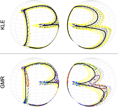
The KLE algorithm is applied using the ESAG distribution on 𝒮2superscript𝒮2\mathcal{S}^{2} as model. The parameters 𝛍^(t)^𝛍𝑡\hat{\bm{\upmu}}(t) and 𝛄^(t)^𝛄𝑡\hat{\bm{\upgamma}}(t) are estimated for 100 equidistant values of t[0,1]𝑡01t\in[0,1] using h=0.010.01h=0.01. The result is shown in the top row of Fig. 4. In order to provide a baseline comparison, the code for Riemannian GMR, available from PbDLib [39], is run for the same dataset 𝒟𝒟\mathscr{D}. The number of stages for the GMR method is fixed to 10. The results are shown in the bottom row of Fig. 4.

An inspection of Fig. 4 shows that the mean (thick black curve) predicted by the KLE method with ESAG model passes through the data more centrally than that predicted by the GMR method. The shape and orientation of the probability level ellipses (yellow curves) predicted by KLE vary more in shape and orientation than those predicted by the GMR, revealing more flexibility in the model.
Refer to caption
Figure 4: Regression for trajectories on 𝒮2superscript𝒮2\mathcal{S}^{2}. TOP: KLE method with ESAG model. BOTTOM: Riemannian GMR with 10 stages, the covariance for each stage is shown in coloured thicker curves.

VI-B Trajectories on Sym+(2)superscriptSym2\mathrm{Sym}^{+}(2) with scalar predictor

In order to test learning of trajectories on the manifold Sym+(d)superscriptSym𝑑\mathrm{Sym}^{+}(d), which was introduced in Sec. II-D, at a dimension that allows visualization of the data, we consider d=2𝑑2d=2. It is desired to obtain a mean and a dispersion structure for new values of the predictor. For this experiment we generate synthetic data, this allows us to have a ground truth against which the results can be compared.

We generate synthetically the set 𝒟={{(𝐱ij,tj)}j=1M}i=1N𝒟superscriptsubscriptsuperscriptsubscriptsubscript𝐱𝑖𝑗subscript𝑡𝑗𝑗1𝑀𝑖1𝑁\mathscr{D}=\{\{(\mathbf{x}_{ij},t_{j})\}_{j=1}^{M}\}_{i=1}^{N}, 𝐱ijSym+(2)subscript𝐱𝑖𝑗superscriptSym2\mathbf{x}_{ij}\in\mathrm{Sym}^{+}(2), tj[0,1]subscript𝑡𝑗01t_{j}\in[0,1]. For every tjsubscript𝑡𝑗t_{j} we simulate the LN distribution, i.e. 𝐱ijLN(𝐌j,𝚺j)similar-tosubscript𝐱𝑖𝑗𝐿𝑁subscript𝐌𝑗subscript𝚺𝑗\mathbf{x}_{ij}\sim LN(\mathbf{M}_{j},\bm{\Sigma}_{j}), j=1,,N𝑗1𝑁j=1,\ldots,N. By controlling the parameters 𝐌jSym+(2)subscript𝐌𝑗superscriptSym2\mathbf{M}_{j}\in\mathrm{Sym}^{+}(2) and 𝚺jSym+(3)subscript𝚺𝑗superscriptSym3\bm{\Sigma}_{j}\in\mathrm{Sym}^{+}(3) we have knowledge of the ground truth.

Consider the spectral decomposition 𝐌j=𝐁(tj)diag(a1(tj),a2(tj))𝐁(tj)subscript𝐌𝑗𝐁subscript𝑡𝑗diagsubscript𝑎1subscript𝑡𝑗subscript𝑎2subscript𝑡𝑗𝐁superscriptsubscript𝑡𝑗top\mathbf{M}_{j}=\mathbf{B}(t_{j})\,\mathrm{diag}(a_{1}(t_{j}),a_{2}(t_{j}))\,\mathbf{B}(t_{j})^{\top}, then 𝐁(t)𝐁𝑡\mathbf{B}(t) and (a1(t),a2(t))subscript𝑎1𝑡subscript𝑎2𝑡(a_{1}(t),a_{2}(t)) are trajectories in SO(2)SO2\mathrm{SO}(2) and 2superscript2\mathbb{R}^{2}, respectively. We generate 𝐁(t)𝐁𝑡\mathbf{B}(t) as planar rotation matrices parametrized by the angle of rotation β(t)𝛽𝑡\beta(t). Then, β(t)𝛽𝑡\beta(t), a1(t)subscript𝑎1𝑡a_{1}(t) and a2(t)subscript𝑎2𝑡a_{2}(t) require simple scalar interpolation.

Similarly, the decomposition 𝚺j=𝐂(tj)diag(b1(tj),b2(tj),b3(tj))𝐂(tj)subscript𝚺𝑗𝐂subscript𝑡𝑗diagsubscript𝑏1subscript𝑡𝑗subscript𝑏2subscript𝑡𝑗subscript𝑏3subscript𝑡𝑗𝐂superscriptsubscript𝑡𝑗top\mathbf{\Sigma}_{j}=\mathbf{C}(t_{j})\,\mathrm{diag}(b_{1}(t_{j}),b_{2}(t_{j}),b_{3}(t_{j}))\,\mathbf{C}(t_{j})^{\top} requires the interpolation of scalars b1(t),b2(t),b3(t)subscript𝑏1𝑡subscript𝑏2𝑡subscript𝑏3𝑡b_{1}(t),b_{2}(t),b_{3}(t)\in\mathbb{R}, while 𝐂(t)O(3)𝐂𝑡O3\mathbf{C}(t)\in\mathrm{O}(3) can be generated by spherical linear interpolation (Slerp) between 𝐂(0)𝐂0\mathbf{C}(0) and 𝐂(1)𝐂1\mathbf{C}(1).

For this particular experiment, for each of M=15𝑀15M=15 equidistant tjsubscript𝑡𝑗t_{j} we generated N=30𝑁30N=30 samples. The following scalar interpolations were considered: a1(t)=(1+9t)2subscript𝑎1𝑡superscript19𝑡2a_{1}(t)=(1+9t)^{2}, a2(t)=(2t)2subscript𝑎2𝑡superscript2𝑡2a_{2}(t)=(2-t)^{2}, β(t)=6.6322t6.2831t2𝛽𝑡6.6322𝑡6.2831superscript𝑡2\beta(t)=6.6322t-6.2831t^{2}, b1(t)=0.2+1.8tsubscript𝑏1𝑡0.21.8𝑡b_{1}(t)=0.2+1.8t, b2(t)=0.15+0.85tsubscript𝑏2𝑡0.150.85𝑡b_{2}(t)=0.15+0.85t and b3(t)=0.1subscript𝑏3𝑡0.1b_{3}(t)=0.1, where β(t)𝛽𝑡\beta(t) was chosen so that β(0)=0𝛽00\beta(0)=0, β(0.5)=100π/180𝛽0.5100𝜋180\beta(0.5)=100\pi/180 and β(1)=20π/180𝛽120𝜋180\beta(1)=20\pi/180. The slerp interpolation for 𝐂(t)𝐂𝑡\mathbf{C}(t) was done between 𝐂(0)=𝐈3𝐂0subscript𝐈3\mathbf{C}(0)=\mathbf{I}_{3} and 𝐂(1)=𝐑Z(15π/180)𝐑Y(5π/180)𝐑X(10π/180)𝐂1subscript𝐑𝑍15𝜋180subscript𝐑𝑌5𝜋180subscript𝐑𝑋10𝜋180\mathbf{C}(1)=\mathbf{R}_{Z}(15\pi/180)\mathbf{R}_{Y}(5\pi/180)\mathbf{R}_{X}(10\pi/180).

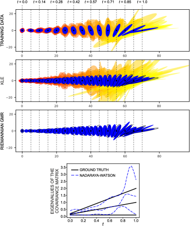
The first plot from top to bottom of Fig. 5 shows 𝒟𝒟\mathscr{D}. The samples are ellipses which are concentric for each value of tjsubscript𝑡𝑗t_{j} and their colour progresses from orange at t0=0subscript𝑡00t_{0}=0 to yellow at t15=1subscript𝑡151t_{15}=1. The 15 means 𝐌jsubscript𝐌𝑗\mathbf{M}_{j} are shown in blue ellipses. We ran the proposed KLE approach with the estimators in Eq. (28) using h=0.060.06h=0.06. We computed 30 queries at equidistant values of t[0,1]𝑡01t\in[0,1]. The results are shown in the second plot of Fig. 5. The estimated mean 𝐌^(t)^𝐌𝑡\hat{\mathbf{M}}(t) is shown in blue ellipses, while the original means, 𝐌jsubscript𝐌𝑗\mathbf{M}_{j}, are superposed in black outline for comparison. For each request, 30 samples are drawn from LN(𝐌^(t),𝚺^(t))𝐿𝑁^𝐌𝑡^𝚺𝑡LN(\hat{\mathbf{M}}(t),\hat{\mathbf{\Sigma}}(t)), their colour progresses from orange (at t=0𝑡0t=0) to yellow (at t=1𝑡1t=1).

It can be seen that the estimated 𝐌^(t)^𝐌𝑡\hat{\mathbf{M}}(t) follows the trend in both shape and orientation of original 𝐌jsubscript𝐌𝑗\mathbf{M}_{j}. The samples drawn from the estimated LN distributions also follow the pattern shown by the training dataset, with an expected slightly larger uncertainty. This uncertainty can be visualised in the bottom plot of Fig. (5), where the eigenvalues of the estimated covariances 𝚺^(t)^𝚺𝑡\hat{\bm{\Sigma}}(t) (dashed blue curves) are plotted against those of the original 𝚺jsubscript𝚺𝑗\bm{\Sigma}_{j}. It can be seen that the uncertainty introduced by the sampling from the original distributions, and the regression process perturb the eigenvalues. However, the trend of those still matches the original ones.

We ran the code for Riemannian GMR available from the PbDLib [39, 40] for the same dataset 𝒟𝒟\mathscr{D} with 10 stages. The results are shown in the third plot of Fig. 5. The estimated mean 𝐌^(t)^𝐌𝑡\hat{\mathbf{M}}(t) is shown in blue ellipses while the original means 𝐌jsubscript𝐌𝑗\mathbf{M}_{j} are the superposed outlined ellipses. It can be seen that the mean follows the trend almost in a similar way to our approach. However, at the end of the trajectory, the mean is more distorted than the one estimated by KLE. Although the Riemannian GMR method uses the same LN distribution as model, we were unable to obtain comparable results for the covariance 𝚺^(t)^𝚺𝑡\hat{\bm{\Sigma}}(t). Hence, its eigenvalues and the samples from the estimated LN distributions are not presented here.
Refer to caption
Figure 5: Learning of trajectories on Sym+(2)superscriptSym2\mathrm{Sym}^{+}(2). FIRST PLOT: Training data 𝒟𝒟\mathscr{D} (orange to yellow) and original mean 𝐌jsubscript𝐌𝑗\mathbf{M}_{j} (blue). SECOND PLOT: Using KLE: estimated mean 𝐌^(t)^𝐌𝑡\hat{\mathbf{M}}(t) (blue), original mean 𝐌jsubscript𝐌𝑗\mathbf{M}_{j} (black outline), and samples from LN(𝐌^(t),𝚺^(t))𝐿𝑁^𝐌𝑡^𝚺𝑡LN(\hat{\mathbf{M}}(t),\hat{\bm{\Sigma}}(t)) (orange to yellow). THIRD PLOT: Using Riemannian GMR: estimated mean 𝐌^(t)^𝐌𝑡\hat{\mathbf{M}}(t) (blue), and original mean 𝐌jsubscript𝐌𝑗\mathbf{M}_{j} (black outline). BOTTOM: eigenvalues of the original covariance matrix 𝚺jsubscript𝚺𝑗\bm{\Sigma}_{j} (solid black), and KLE-computed 𝚺^(t)^𝚺𝑡\hat{\bm{\Sigma}}(t) (dashed blue)

VI-C Trajectories on SE(3)SE3\mathrm{SE(3)} with scalar predictor

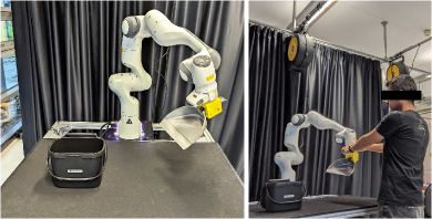
In this experiment, we teach a Franka Emika Panda arm with a dustpan attached to its end-effector to drop rubbish into the bin, see Fig. 6 (left). The demonstrated trajectories involve large changes in the orientation of the end-effector frame. We carried out kinesthetic demonstrations (Fig. 6) and tracked the pose of the end-effector frame E𝐸E in world frame O𝑂O. Thus, we generate the dataset 𝒟={{(𝐱ij,𝐩ij,tij)}j=1Mi}i=1N𝒟superscriptsubscriptsuperscriptsubscriptsubscript𝐱𝑖𝑗subscript𝐩𝑖𝑗subscript𝑡𝑖𝑗𝑗1subscript𝑀𝑖𝑖1𝑁\mathscr{D}=\{\{(\mathbf{x}_{ij},\mathbf{p}_{ij},t_{ij})\}_{j=1}^{M_{i}}\}_{i=1}^{N}, where 𝐱ij𝒮3/2subscript𝐱𝑖𝑗superscript𝒮3subscript2\mathbf{x}_{ij}\in\mathcal{S}^{3}/\mathbb{Z}_{2} is the quaternion representation of the orientation, 𝐩ij3subscript𝐩𝑖𝑗superscript3\mathbf{p}_{ij}\in\mathbb{R}^{3} is the position, and tj[0,1]subscript𝑡𝑗01t_{j}\in[0,1] is the normalized time. For this experiment, we considered N=12𝑁12N=12 demonstrations, and we randomly sampled Mi=80subscript𝑀𝑖80M_{i}=80, ifor-all𝑖\forall i, points from each recorded trajectory.

The left side of Fig. 7 shows the orientation set {{(𝐱ij,tij)}j=1Mi}i=1Nsuperscriptsubscriptsuperscriptsubscriptsubscript𝐱𝑖𝑗subscript𝑡𝑖𝑗𝑗1subscript𝑀𝑖𝑖1𝑁\{\{(\mathbf{x}_{ij},t_{ij})\}_{j=1}^{M_{i}}\}_{i=1}^{N}. Since 𝐱ijsubscript𝐱𝑖𝑗\mathbf{x}_{ij} is axial data, we ran a KLE algorithm with an ACG distribution as model. For 200 equidistant values of t[0,1]𝑡01t\in[0,1], we estimated the parameter 𝚲^(t)^𝚲𝑡\hat{\bm{\Lambda}}(t) using the solution for KLE in Eq. (18). We used h=0.040.04h=0.04, and the Rao-Fisher metric (see, for example, Eq. (10) in [42]) to stop the iterations in Eq. (18) with a threshold of 1×1041superscript1041\times 10^{-4}. Due to the redundancy of 𝚲𝚲\bm{\Lambda}, we normalised it so that tr(𝚲^(t))=4tr^𝚲𝑡4\mathrm{tr}(\hat{\bm{\Lambda}}(t))=4, tfor-all𝑡\forall t. The right-hand side of Fig. 7 shows the mean, 𝐛^(1)(t)subscript^𝐛1𝑡\hat{\mathbf{b}}_{(1)}(t), i.e. the eigenvector associated with the largest eigenvalue. In order to have a sense of density levels, for each t𝑡t, ACG(𝚲^(t))𝐴𝐶𝐺^𝚲𝑡ACG(\hat{\bm{\Lambda}}(t)) is simulated with 350 samples, then the 140 with the highest density (Eq. (16)) are plotted in Fig. 7. It can be seen that the density follows the trend of the training data.

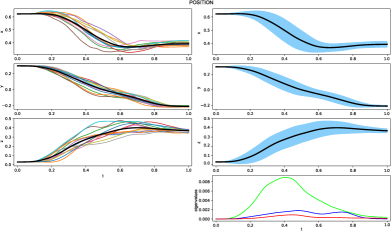
The left side of Fig. 8 shows the position set {{(𝐩ij,tij)}j=1Mi}i=1Nsuperscriptsubscriptsuperscriptsubscriptsubscript𝐩𝑖𝑗subscript𝑡𝑖𝑗𝑗1subscript𝑀𝑖𝑖1𝑁\{\{(\mathbf{p}_{ij},t_{ij})\}_{j=1}^{M_{i}}\}_{i=1}^{N}. Since 𝐩ij3subscript𝐩𝑖𝑗superscript3\mathbf{p}_{ij}\in\mathbb{R}^{3}, the task is much simpler and we ran a KLE algorithm with a multivariate Gaussian distribution as model. We used Eq. (14) to determine 𝛍(t)𝛍𝑡\bm{\upmu}(t) and 𝚺(t)𝚺𝑡\bm{\Sigma}(t), respectively. The results are shown on the right-hand side of Fig. 8.
Refer to caption
Figure 6: LEFT: Setup for experiment in Section VI-C – a Franka Panda arm with a dustpan as end-effector, and a bin on the table. RIGHT: A participant carries out a kinesthetic demonstration.
Refer to caption
Figure 7: LEFT: Orientations of demonstrations 𝒟𝒟\mathscr{D}, i.e. dataset {{(𝐱ij,tij)}j=1Mi}i=1Nsuperscriptsubscriptsuperscriptsubscriptsubscript𝐱𝑖𝑗subscript𝑡𝑖𝑗𝑗1subscript𝑀𝑖𝑖1𝑁\{\{(\mathbf{x}_{ij},t_{ij})\}_{j=1}^{M_{i}}\}_{i=1}^{N}, 𝐱ij=(xij,yij,zij,wij)𝒮3/2subscript𝐱𝑖𝑗subscript𝑥𝑖𝑗subscript𝑦𝑖𝑗subscript𝑧𝑖𝑗subscript𝑤𝑖𝑗superscript𝒮3subscript2\mathbf{x}_{ij}=(x_{ij},y_{ij},z_{ij},w_{ij})\in\mathcal{S}^{3}/\mathbb{Z}_{2}. RIGHT: Mean 𝐛^(1)(t)subscript^𝐛1𝑡\hat{\mathbf{b}}_{(1)}(t) and density level by sampling, see text for details. RIGHT-BOTTOM: second through fourth eigenvalues of 𝚲(t)𝚲𝑡\bm{\Lambda}(t)

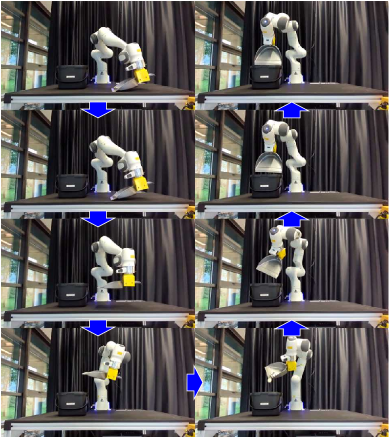
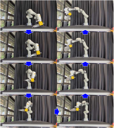
Fig. 9 shows stills of the robot executing the mean trajectory {(𝐛^(1)(tk),𝛍^(tk),tk)}k=1200subscriptsuperscriptsubscript^𝐛1subscript𝑡𝑘^𝛍subscript𝑡𝑘subscript𝑡𝑘200𝑘1\{(\hat{\mathbf{b}}_{(1)}(t_{k}),\hat{\bm{\upmu}}(t_{k}),t_{k})\}^{200}_{k=1}. Fig. 10 shows several curves generated following the method proposed in Section IV-D. The curves are generated by smoothing through 120 points from the set {(𝐱k,tk)}k=1120subscriptsuperscriptsubscript𝐱𝑘subscript𝑡𝑘120𝑘1\{(\mathbf{x}_{k},t_{k})\}^{120}_{k=1}, 𝐱kACG(𝚲^(tk))similar-tosubscript𝐱𝑘𝐴𝐶𝐺^𝚲subscript𝑡𝑘\mathbf{x}_{k}\sim ACG(\hat{\bm{\Lambda}}(t_{k})), for orientation, and {(𝐩k,tk)}k=1120subscriptsuperscriptsubscript𝐩𝑘subscript𝑡𝑘120𝑘1\{(\mathbf{p}_{k},t_{k})\}^{120}_{k=1}, 𝐩k𝒩(𝛍^(tk),𝚺^(tk))similar-tosubscript𝐩𝑘𝒩^𝛍subscript𝑡𝑘^𝚺subscript𝑡𝑘\mathbf{p}_{k}\sim\mathcal{N}(\hat{\bm{\upmu}}(t_{k}),\hat{\bm{\Sigma}}(t_{k})).

Refer to caption
Figure 8: LEFT: Positions of demonstrations 𝒟𝒟\mathscr{D}, i.e. dataset {{(𝐩ij,tij)}j=1Mi}i=1Nsuperscriptsubscriptsuperscriptsubscriptsubscript𝐩𝑖𝑗subscript𝑡𝑖𝑗𝑗1subscript𝑀𝑖𝑖1𝑁\{\{(\mathbf{p}_{ij},t_{ij})\}_{j=1}^{M_{i}}\}_{i=1}^{N}, 𝐩ij=(xij,yij,zij)3subscript𝐩𝑖𝑗subscript𝑥𝑖𝑗subscript𝑦𝑖𝑗subscript𝑧𝑖𝑗superscript3\mathbf{p}_{ij}=(x_{ij},y_{ij},z_{ij})\in\mathbb{R}^{3}. RIGHT: Mean 𝛍^(t)^𝛍𝑡\hat{\bm{\upmu}}(t) with 1.5 standard deviation density level. RIGHT-BOTTOM: eigenvalues of 𝚺^(t)^𝚺𝑡\hat{\bm{\Sigma}}(t)
Refer to caption
Figure 9: Franka Panda arm following the mean task-space trajectory obtained from 𝒟𝒟\mathscr{D}. See video in the supplementary material.

It is now desired to adapt the learnt trajectories after the bin has been moved to a new pose. The final pose of the end-effector, 𝐓EOsuperscriptsubscriptsuperscript𝐓𝐸𝑂{}^{O}_{E}\mathbf{T}^{*}, that will allow dropping the rubbish in the bin in its new pose is known. It is known that frame E𝐸E must be at a new orientation with quaternion representation 𝐱T=(0.821,0.342,0.243,0.386)subscriptsuperscript𝐱𝑇superscript0.8210.3420.2430.386top\mathbf{x}^{*}_{T}=(0.821,0.342,-0.243,-0.386)^{\top}, and new position 𝐩T=(0.237,0.520,0.343)subscriptsuperscript𝐩𝑇0.2370.5200.343\mathbf{p}^{*}_{T}=(0.237,-0.520,0.343). We followed the method presented in Section IV-C. For the orientation part we used activation functions α(t)=0.50.5tanh(3t2.4)𝛼𝑡0.50.53𝑡2.4\alpha(t)=0.5-0.5\tanh(3t-2.4) and β(t)=1α(t)𝛽𝑡1𝛼𝑡\beta(t)=1-\alpha(t). The dataset ={{(𝐲ij,tj)}j=180}i=112superscriptsubscriptsuperscriptsubscriptsubscript𝐲𝑖𝑗subscript𝑡𝑗𝑗180𝑖112\mathscr{E}=\{\{(\mathbf{y}_{ij},t_{j})\}_{j=1}^{80}\}_{i=1}^{12} is generated by sampling, for every tjsubscript𝑡𝑗t_{j}, {𝐲ij}i=112superscriptsubscriptsuperscriptsubscript𝐲𝑖𝑗𝑖112\{\mathbf{y}_{ij}^{*}\}_{i=1}^{12}, 𝐲ijACG(𝚲)similar-tosuperscriptsubscript𝐲𝑖𝑗𝐴𝐶𝐺superscript𝚲\mathbf{y}_{ij}^{*}\sim ACG(\bm{\Lambda}^{*}), where 𝚲=𝐁𝐀(𝐁)superscript𝚲superscript𝐁superscript𝐀superscriptsuperscript𝐁top\bm{\Lambda}^{*}=\mathbf{B}^{*}\mathbf{A}^{*}(\mathbf{B}^{*})^{\top}. For a low uncertainty at the adapted point, we set 𝐀=diag(1×105,1,1,1)superscript𝐀diag1superscript105111\mathbf{A}^{*}=\mathrm{diag}(1\times 10^{5},1,1,1). While 𝐁superscript𝐁\mathbf{B}^{*} is obtained computing an orthonormal basis for the complement space of 𝐱Tsuperscriptsubscript𝐱𝑇\mathbf{x}_{T}^{*} to 4superscript4\mathbb{R}^{4}. The position part is done similarly with samples being drawn from 𝒩(𝐩T,1×105𝐈3)𝒩subscriptsuperscript𝐩𝑇1superscript105subscript𝐈3\mathcal{N}(\mathbf{p}^{*}_{T},1\times 10^{-5}\mathbf{I}_{3}), and first activation function α(t)=0.50.5tanh(13t6.5)𝛼𝑡0.50.513𝑡6.5\alpha(t)=0.5-0.5\tanh(13t-6.5).

The results of this adaptation process are shown in Fig. 11. It can be seen that the means achieve the desired new pose at the end of the trajectory. It can also be seen that the distributions for both position and orientation become highly concentrated at the end of the trajectory. Fig. 12 shows the robot following the adapted mean.
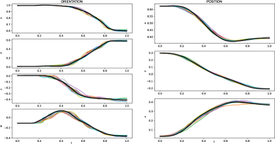
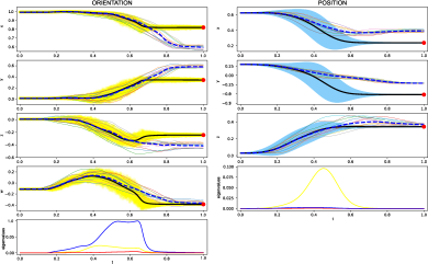
Refer to caption
Figure 10: Ten trajectories generated from the learnt model using the method presented in Section IV-D
Refer to caption
Figure 11: Adaptation of the learnt trajectories. 𝐱Fsubscriptsuperscript𝐱𝐹\mathbf{x}^{*}_{F} and 𝐩Fsubscriptsuperscript𝐩𝐹\mathbf{p}^{*}_{F} are shown in red dots. The adapted mean is shown in thick black curve. The yellow density levels of the orientation part are obtained by sampling, while the ones for position represent 1.5 covariance levels. The original trajectories of 𝒟𝒟\mathscr{D} are also shown as is their mean, in dashed thick curves. The bottom-left plot shows the second through fourth eigenvalues of 𝚲(t)𝚲𝑡\bm{\Lambda}(t), while the bottom-right shows the eigenvalues of 𝚺(t)𝚺𝑡\bm{\Sigma}(t)
Refer to caption
Figure 12: Franka Panda arm following the adapted task-space trajectory after the bin has been moved. See video in the supplementary material.

VI-D Regression with response in Sym+(6)superscriptSym6\mathrm{Sym}^{+}(6) and predictor in 2×𝒮1superscript2superscript𝒮1\mathbb{R}^{2}\times\mathcal{S}^{1}

In this experiment, simple regression (rather than trajectory learning) is carried out using the KLE method. The predictor is on a manifold, 2×𝒮1superscript2superscript𝒮1\mathbb{R}^{2}\times\mathcal{S}^{1}, which represents the position and orientation of a paint roller on a wall, while the response is in Sym+(6)superscriptSym6\mathrm{Sym}^{+}(6), representing the manipulability ellipsoid of a demonstrator holding the paint roller. Such manipulability will be then transferred to the robot. This should be reflected in a more human posture.

A 7-DOF Franka Emika Panda arm is to be taught to hold a paint roller against the wall with the manipulability that a human would impose. The demonstrations are a set of postures of a human holding a roller at different positions and orientations of the roller on a wall. For a new position and orientation of the roller, it is desired to predict the manipulability ellipsoid that the human would impose and, subsequently, transfer this to the robot. We assume that the angle that the handle of the roller makes with the wall is constant. Therefore, the predictor of this regression problem is in 2×𝒮1superscript2superscript𝒮1\mathbb{R}^{2}\times\mathcal{S}^{1} (position and orientation of the roller on the wall) and the response is in Sym+(6)superscriptSym6\mathrm{Sym}^{+}(6) (manipulability ellipsoid). Since, in this case, the rotation axis of the roller is perpendicular to its translation, 2×𝒮1superscript2superscript𝒮1\mathbb{R}^{2}\times\mathcal{S}^{1} parametrises the group of planar displacements, P(3)P3\mathrm{P}(3) [32]. This is a 3-dimensional subgroup of SE(3)SE3\mathrm{SE}(3) and is sometimes also referred to as SE(2)SE2\mathrm{SE}(2).

Note that, unlike [17] and [18], we are not interested in tracking manipulability from human to robot along a trajectory. Instead, we only aim to transfer the estimated manipulability for a single pose of the end-effector which puts the roller on the wall with a desired position and orientation.

The training dataset for this experiment is 𝒟={(𝐗i,𝐩i,ϕi)}i=1N𝒟superscriptsubscriptsubscript𝐗𝑖subscript𝐩𝑖subscriptitalic-ϕ𝑖𝑖1𝑁\mathscr{D}=\{(\mathbf{X}_{i},\mathbf{p}_{i},\phi_{i})\}_{i=1}^{N}, where 𝐗iSym+(6)subscript𝐗𝑖superscriptSym6\mathbf{X}_{i}\in\mathrm{Sym}^{+}(6), 𝐩i2subscript𝐩𝑖superscript2\mathbf{p}_{i}\in\mathbb{R}^{2}, ϕi𝒮1subscriptitalic-ϕ𝑖superscript𝒮1\phi_{i}\in\mathcal{S}^{1}.

We tracked the right arm of a participant using a Vicon System as shown in Fig. 13 (top). For each demonstration i𝑖i we obtained the manipulability ellipsoid of the right arm from its Jacobian matrix as 𝐗i=𝐉H,i𝐉H,isubscript𝐗𝑖subscript𝐉𝐻𝑖superscriptsubscript𝐉𝐻𝑖top\mathbf{X}_{i}=\mathbf{J}_{H,i}\mathbf{J}_{H,i}^{\top}. To obtain 𝐉H,isubscript𝐉𝐻𝑖\mathbf{J}_{H,i}, we use the kinematic model shown in Fig. 13 (bottom). The model is a 7-DOF kinematic chain and was previously used in several publications [43, 44, 45]. The Vicon world frame V𝑉V is fixed so that the wall coincides with the yVzVsubscript𝑦𝑉subscript𝑧𝑉y_{V}\text{--}z_{V} plane. Frame B𝐵B is the recommended by the International Society of Biomechanics [46] as thorax coordinate system.

Let 𝐒jsubscript𝐒𝑗\mathbf{S}_{j} be the screw axis of joint j𝑗j, then the geometry of the kinematic chain modelling the arm is fully defined by the following constraints: 𝐒1subscript𝐒1\mathbf{S}_{1}, 𝐒2subscript𝐒2\mathbf{S}_{2} and 𝐒3subscript𝐒3\mathbf{S}_{3} intersect at CSsubscript𝐶𝑆C_{S}, the shoulder centre. Similarly, 𝐒5subscript𝐒5\mathbf{S}_{5}, 𝐒6subscript𝐒6\mathbf{S}_{6} and 𝐒7subscript𝐒7\mathbf{S}_{7} intersect at CWsubscript𝐶𝑊C_{W}, the wrist centre. 𝐒4subscript𝐒4\mathbf{S}_{4} passes through CEsubscript𝐶𝐸C_{E}, the elbow centre. 𝐒1subscript𝐒1\mathbf{S}_{1} is antiparallel to yBsubscript𝑦𝐵y_{B}, 𝐒3subscript𝐒3\mathbf{S}_{3} is coincident with line CSCE¯¯subscript𝐶𝑆subscript𝐶𝐸\overline{C_{S}C_{E}}, and 𝐒2subscript𝐒2\mathbf{S}_{2} is perpendicular to 𝐒1subscript𝐒1\mathbf{S}_{1} and 𝐒3subscript𝐒3\mathbf{S}_{3}. 𝐒5subscript𝐒5\mathbf{S}_{5} is coincident with line CECW¯¯subscript𝐶𝐸subscript𝐶𝑊\overline{C_{E}C_{W}}, 𝐒4subscript𝐒4\mathbf{S}_{4} is perpendicular to 𝐒3subscript𝐒3\mathbf{S}_{3} and 𝐒5subscript𝐒5\mathbf{S}_{5}. 𝐒7subscript𝐒7\mathbf{S}_{7} is perpendicular to 𝐡Fsubscript𝐡𝐹\mathbf{h}_{F} and 𝐡Psubscript𝐡𝑃\mathbf{h}_{P}, which are the directions of the middle finger, and the normal to the palm, respectively. Finally, 𝐒6subscript𝐒6\mathbf{S}_{6} is perpendicular to 𝐒5subscript𝐒5\mathbf{S}_{5} and 𝐒7subscript𝐒7\mathbf{S}_{7}.

Refer to caption
Figure 13: Data collection for experiment VI-D. TOP: A participant demonstrates how he holds a roller against a wall. The wall is a net of threads to allow the cameras track the markers. The markers set is defined for tracking of the joint centres, and thorax and roller frames. BOTTOM: Kinematic model and related coordinate systems for right arm holding a paint roller.

If 𝐒jse(3)subscript𝐒𝑗se3\mathbf{S}_{j}\in\mathrm{se}(3) are the Plücker coordinates of the joint axes [47], the Jacobian matrix is given by 𝐉H=[𝐒1,,𝐒7]6×7subscript𝐉𝐻subscript𝐒1subscript𝐒7superscript67\mathbf{J}_{H}=[\mathbf{S}_{1},\ldots,\mathbf{S}_{7}]\in\mathbb{R}^{6\times 7}. We track a frame R𝑅R fixed to the roller, as shown in Fig. 13. As claimed before, we assume that the angle between axis yRsubscript𝑦𝑅y_{R} and the wall, i.e. plane yVzVsubscript𝑦𝑉subscript𝑧𝑉y_{V}\text{--}z_{V}, is constant. We also assume that the distance between the shoulder centre, CSsubscript𝐶𝑆C_{S}, and the wall remains unchanged between demonstrations. Then, our predictor variables (𝐩,ϕ)2×𝒮1𝐩italic-ϕsuperscript2superscript𝒮1(\mathbf{p},\phi)\in\mathbb{R}^{2}\times\mathcal{S}^{1} are defined as:

  • 𝐩2𝐩superscript2\mathbf{p}\in\mathbb{R}^{2} is the projection of vector 𝐫ORB𝐫CSBsuperscriptsubscript𝐫subscript𝑂𝑅𝐵superscriptsubscript𝐫subscript𝐶𝑆𝐵{}^{B}\mathbf{r}_{O_{R}}-{}^{B}\mathbf{r}_{C_{S}} onto the wall (plane yVzVsubscript𝑦𝑉subscript𝑧𝑉y_{V}\text{--}z_{V}).

  • ϕ𝒮1italic-ϕsuperscript𝒮1\phi\in\mathcal{S}^{1} is the angle between xRsubscript𝑥𝑅x_{R} and yVsubscript𝑦𝑉y_{V} about xVsubscript𝑥𝑉-x_{V}.

A total of N=80𝑁80N=80 demonstrations were obtained. Then the KLE algorithm was used to predict a manipulability ellipsoid for a new pair (𝐩,ϕ)2×𝒮1𝐩italic-ϕsuperscript2superscript𝒮1(\mathbf{p},\phi)\in\mathbb{R}^{2}\times\mathcal{S}^{1}. This is done by modifying the metric in the kernel of Eq. (28). The estimator is then:

𝐌^(𝐩,ϕ)=exp{i=1NKh(dP(3)((𝐩i,ϕi),(𝐩,ϕ)))log(𝐗i)i=1NKh(dP(3)((𝐩i,ϕi),(𝐩,ϕ)))}^𝐌𝐩italic-ϕexpsuperscriptsubscript𝑖1𝑁subscript𝐾subscript𝑑P3subscript𝐩𝑖subscriptitalic-ϕ𝑖𝐩italic-ϕlogsubscript𝐗𝑖superscriptsubscript𝑖1𝑁subscript𝐾subscript𝑑P3subscript𝐩𝑖subscriptitalic-ϕ𝑖𝐩italic-ϕ\hat{\mathbf{M}}(\mathbf{p},\phi)=\mathrm{exp}\left\{\sum_{i=1}^{N}\dfrac{K_{h}\Big{(}d_{\mathrm{P}(3)}\big{(}(\mathbf{p}_{i},\phi_{i}),(\mathbf{p},\phi)\big{)}\Big{)}\mathrm{log}(\mathbf{X}_{i})}{\sum\limits_{i=1}^{N}K_{h}\Big{(}d_{\mathrm{P}(3)}\big{(}(\mathbf{p}_{i},\phi_{i}),(\mathbf{p},\phi)\big{)}\Big{)}}\right\}

where dP(3)()subscript𝑑P3d_{\mathrm{P}(3)}(\cdot) is a metric in P(3)P3\mathrm{P}(3). Just like in SE(3)SE3\mathrm{SE}(3), the lack of a natural length scale in P(3)P3\mathrm{P}(3) does not allow for the introduction of a bi-invariant metric. Hence, as suggested in [48], a distance of weighted form is used:

dP(3)((𝐩i,ϕi),(𝐩,ϕ)):=wϕdϕ(ϕi,ϕ)+wpdp(𝐩i,𝐩),assignsubscript𝑑P3subscript𝐩𝑖subscriptitalic-ϕ𝑖𝐩italic-ϕsubscript𝑤italic-ϕsubscript𝑑italic-ϕsubscriptitalic-ϕ𝑖italic-ϕsubscript𝑤𝑝subscript𝑑𝑝subscript𝐩𝑖𝐩d_{\mathrm{P}(3)}\left((\mathbf{p}_{i},\phi_{i}),(\mathbf{p},\phi)\right):=w_{\phi}d_{\phi}(\phi_{i},\phi)+w_{p}d_{p}(\mathbf{p}_{i},\mathbf{p}),

where dϕ()subscript𝑑italic-ϕd_{\phi}(\cdot) is a metric in 𝒮1superscript𝒮1\mathcal{S}^{1} (smallest angle) and dp()subscript𝑑𝑝d_{p}(\cdot) is simply the Euclidean distance in 2superscript2\mathbb{R}^{2}. Similarly to [49], we define such weights considering the averages of distances in the rotational and translational data to their respective means:

wpsubscript𝑤𝑝\displaystyle w_{p} :=assign\displaystyle:= (1Ni=1N𝐩¯P𝐩i)1,superscript1𝑁superscriptsubscript𝑖1𝑁normsubscript¯𝐩𝑃subscript𝐩𝑖1\displaystyle\left(\frac{1}{N}\sum\limits_{i=1}^{N}\|\overline{\mathbf{p}}_{P}-\mathbf{p}_{i}\|\right)^{-1},
wϕsubscript𝑤italic-ϕ\displaystyle w_{\phi} :=assign\displaystyle:= (1Ni=1Ndϕ(ϕ¯,ϕi))1,superscript1𝑁superscriptsubscript𝑖1𝑁subscript𝑑italic-ϕ¯italic-ϕsubscriptitalic-ϕ𝑖1\displaystyle\left(\frac{1}{N}\sum\limits_{i=1}^{N}d_{\phi}(\overline{\phi},\phi_{i})\right)^{-1},

where ϕ¯¯italic-ϕ\overline{\phi} is the mean for circular data in Eq. (2.2.4) of [26]. Alternatively, [50] suggests wp=1subscript𝑤𝑝1w_{p}=1 and wϕsubscript𝑤italic-ϕw_{\phi} equal to the largest distance between two points of the projection of the rigid body onto the displacement plane. In our case, such a distance is the axial length of the roller, 0.23m. We tested this metric with very similar results.

It is now necessary to transfer 𝐌^(𝐩,ϕ)^𝐌𝐩italic-ϕ\hat{\mathbf{M}}(\mathbf{p},\phi) to the robot. Since we are only interested in the proportion and orientation of the manipulability ellipsoid, we normalize the response as 𝐗H:=𝐌^(𝐩,ϕ)/λH,maxassignsubscript𝐗𝐻^𝐌𝐩italic-ϕsubscript𝜆𝐻max\mathbf{X}_{H}:=\hat{\mathbf{M}}(\mathbf{p},\phi)/\lambda_{H,\mathrm{max}}, where λH,maxsubscript𝜆𝐻max\lambda_{H,\mathrm{max}} is the largest eigenvalue of 𝐌^(𝐩,ϕ)^𝐌𝐩italic-ϕ\hat{\mathbf{M}}(\mathbf{p},\phi).

Since 𝐓ROsuperscriptsubscript𝐓𝑅𝑂{}^{O}_{R}\mathbf{T}, the pose of the roller frame R𝑅R, is fully defined by a requested (𝐩,ϕ)𝐩italic-ϕ(\mathbf{p},\phi), and since, once the roller is attached to the end-effector of the robot, the transformation 𝐓REsuperscriptsubscript𝐓𝑅𝐸{}^{E}_{R}\mathbf{T} is known, then (𝐩,ϕ)𝐩italic-ϕ(\mathbf{p},\phi) defines a unique pose of the end-effector, 𝐓EO=𝐓RO(𝐩,ϕ)(𝐓RE)1superscriptsubscript𝐓𝐸𝑂superscriptsubscript𝐓𝑅𝑂𝐩italic-ϕsuperscriptsuperscriptsubscript𝐓𝑅𝐸1{}^{O}_{E}\mathbf{T}={}^{O}_{R}\mathbf{T}(\mathbf{p},\phi)({}^{E}_{R}\mathbf{T})^{-1}.

After a pose of the end-effector is defined by a requested (𝐩,ϕ)𝐩italic-ϕ(\mathbf{p},\phi), the 1-DOF redundancy of the robot gives us one free parameter that allows us to adjust the manipulability ellipsoid of the Franka arm, which we normalise as 𝐗F:=𝐉F𝐉F/λF,maxassignsubscript𝐗𝐹subscript𝐉𝐹superscriptsubscript𝐉𝐹topsubscript𝜆𝐹max\mathbf{X}_{F}:=\mathbf{J}_{F}\mathbf{J}_{F}^{\top}/\lambda_{F,\mathrm{max}}, where λF,maxsubscript𝜆𝐹max\lambda_{F,\mathrm{max}} is the largest eigenvalue of 𝐉F𝐉Fsubscript𝐉𝐹superscriptsubscript𝐉𝐹top\mathbf{J}_{F}\mathbf{J}_{F}^{\top}. 𝐗Fsubscript𝐗𝐹\mathbf{X}_{F} is optimised to be as close as possible to 𝐗Hsubscript𝐗𝐻\mathbf{X}_{H}. To this end, we use the analytical solution for the inverse kinematics (IK) of the Franka Panda arm based on [51]. This IK function has as input the end-effector pose, 𝐓EOsuperscriptsubscript𝐓𝐸𝑂{}^{O}_{E}\mathbf{T}, and a value of the seventh joint angle, q7[q7,MIN,q7,MAX]subscript𝑞7subscript𝑞7MINsubscript𝑞7MAXq_{7}\in[q_{7,\mathrm{MIN}},q_{7,\mathrm{MAX}}], as free parameter. The function returns a maximum of 8 solutions 𝐪𝕋7𝐪superscript𝕋7\mathbf{q}\in\mathbb{T}^{7}. Therefore, for a given 𝐓EOsuperscriptsubscript𝐓𝐸𝑂{}^{O}_{E}\mathbf{T}, we consider the Jacobian matrix as a function of q7subscript𝑞7q_{7} alone. Thus, we are interested in the maximiser:

q7#=argminq7dSPD(𝐗H,𝐗F(q7)),superscriptsubscript𝑞7#subscriptsubscript𝑞7subscript𝑑SPDsubscript𝐗𝐻subscript𝐗𝐹subscript𝑞7q_{7}^{\#}=\arg\min_{q_{7}}d_{\mathrm{SPD}}\left(\mathbf{X}_{H},\,\mathbf{X}_{F}(q_{7})\right), (30)

where dSPD()subscript𝑑SPDd_{\mathrm{SPD}}(\cdot) is a metric in Sym+(6)superscriptSym6\mathrm{Sym}^{+}(6). For these experiments, we chose the Rao-Fisher metric.

Since this is a 1-dimensional bounded search, the optimization in Eq. (30) can be simply done by discretising [q7,MIN[q_{7,\mathrm{MIN}}, q7,MAX]\,q_{7,\mathrm{MAX}}], calculating the IK for each angle and picking the one that minimizes (30). Since our IK is analytical, this process much faster than what it would be if we used any of the numerical IK solvers, which are the commonplace for 7-DOF robots.

We ran the experiment for a requested pose of the roller (𝐩,ϕ)=((0.20,0.55),π/6)𝐩italic-ϕ0.200.55𝜋6(\mathbf{p},\phi)=((-0.20,0.55),\pi/6). We set h=0.260.26h=0.26 from cross-validation. The estimated 𝐗Hsubscript𝐗𝐻\mathbf{X}_{H} and transferred 𝐗Fsubscript𝐗𝐹\mathbf{X}_{F} have the following eigenvalues:

λ(𝐗H)=(1, 0.821, 0.657, 0.059, 0.035, 0.003),𝜆subscript𝐗𝐻10.8210.6570.0590.0350.003\displaystyle\lambda(\mathbf{X}_{H})=(1,\,0.821,\,0.657,\,0.059,\,0.035,\,0.003),
λ(𝐗F)=(1, 0.722, 0.524, 0.058, 0.043, 0.007),𝜆subscript𝐗𝐹10.7220.5240.0580.0430.007\displaystyle\lambda(\mathbf{X}_{F})=(1,\,0.722,\,0.524,\,0.058,\,0.043,\,0.007),

with corresponding eigenvectors:

eig(𝐗H)={[0.6340.4570.5300.0430.2060.252],[0.7650.4040.4770.0390.1280.077],[0.0290.6880.6080.1550.2070.298],[0.0250.0800.0060.8550.3560.367],[0.0410.0160.3470.3450.8700.034],[0.0970.3840.0300.3490.1200.840]}eigsubscript𝐗𝐻delimited-[]0.6340.4570.5300.0430.2060.252delimited-[]0.7650.4040.4770.0390.1280.077delimited-[]0.0290.6880.6080.1550.2070.298delimited-[]0.0250.0800.0060.8550.3560.367delimited-[]0.0410.0160.3470.3450.8700.034delimited-[]0.0970.3840.0300.3490.1200.840\begin{split}\mathrm{eig}(\mathbf{X}_{H})&=\left\{\left[\begin{array}[]{c}-0.634\\ -0.457\\ 0.530\\ -0.043\\ -0.206\\ -0.252\end{array}\right],\left[\begin{array}[]{c}-0.765\\ 0.404\\ -0.477\\ 0.039\\ 0.128\\ 0.077\end{array}\right],\left[\begin{array}[]{c}0.029\\ -0.688\\ -0.608\\ 0.155\\ 0.207\\ -0.298\end{array}\right],\right.\\ &\qquad\left.\left[\begin{array}[]{c}-0.025\\ -0.080\\ 0.006\\ 0.855\\ -0.356\\ 0.367\end{array}\right],\left[\begin{array}[]{c}-0.041\\ 0.016\\ 0.347\\ 0.345\\ 0.870\\ 0.034\end{array}\right],\left[\begin{array}[]{c}-0.097\\ -0.384\\ -0.030\\ -0.349\\ 0.120\\ 0.840\end{array}\right]\right\}\end{split}
eig(𝐗F)={[0.1380.0950.9360.0770.2980.045],[0.9850.0530.1590.0190.0160.044],[0.0720.9630.0740.0730.0580.229],[0.0410.0360.0560.9120.0880.392],[0.0630.0770.2970.1400.9260.158],[0.0310.2290.0490.3700.2060.874]}eigsubscript𝐗𝐹delimited-[]0.1380.0950.9360.0770.2980.045delimited-[]0.9850.0530.1590.0190.0160.044delimited-[]0.0720.9630.0740.0730.0580.229delimited-[]0.0410.0360.0560.9120.0880.392delimited-[]0.0630.0770.2970.1400.9260.158delimited-[]0.0310.2290.0490.3700.2060.874\begin{split}\mathrm{eig}(\mathbf{X}_{F})&=\left\{\left[\begin{array}[]{c}-0.138\\ -0.095\\ 0.936\\ -0.077\\ -0.298\\ -0.045\end{array}\right],\left[\begin{array}[]{c}0.985\\ 0.053\\ 0.159\\ 0.019\\ 0.016\\ 0.044\end{array}\right],\left[\begin{array}[]{c}0.072\\ -0.963\\ -0.074\\ 0.073\\ 0.058\\ -0.229\end{array}\right],\right.\\ &\qquad\left.\left[\begin{array}[]{c}-0.041\\ -0.036\\ 0.056\\ 0.912\\ -0.088\\ 0.392\end{array}\right],\left[\begin{array}[]{c}-0.063\\ 0.077\\ 0.297\\ 0.140\\ 0.926\\ -0.158\end{array}\right],\left[\begin{array}[]{c}-0.031\\ -0.229\\ 0.049\\ -0.370\\ 0.206\\ 0.874\end{array}\right]\right\}\end{split}

Eq. (30) returned q7#=1.412superscriptsubscript𝑞7#1.412q_{7}^{\#}=1.412, with 𝐪#=(0.886,1.651,2.154,1.528,2.322,2.165,1.412)superscript𝐪#0.8861.6512.1541.5282.3222.1651.412\mathbf{q}^{\#}=(-0.886,1.651,2.154,-1.528,2.322,2.165,1.412) as whole configuration of the arm. The corresponding position and orientation ellipsoids for 𝐗Fsubscript𝐗𝐹\mathbf{X}_{F} and 𝐗Hsubscript𝐗𝐻\mathbf{X}_{H} are shown in Fig. 14.

Refer to caption
Figure 14: Position and orientation ellipsoids for 𝐗Hsubscript𝐗𝐻\mathbf{X}_{H} (red) and 𝐗Fsubscript𝐗𝐹\mathbf{X}_{F} (blue)
Refer to caption
Figure 15: The Franka Panda arm is initially in a home configuration 𝐪0subscript𝐪0\mathbf{q}_{0} (LEFT). Then 𝐪#superscript𝐪#\mathbf{q}^{\#}, which optimises 𝐗Fsubscript𝐗𝐹\mathbf{X}_{F} to be as close as possible to 𝐗H(𝐩,ϕ)subscript𝐗𝐻𝐩italic-ϕ\mathbf{X}_{H}(\mathbf{p},\phi) is set as as joint goal on Moveit! This takes the robot to 𝐪#superscript𝐪#\mathbf{q}^{\#} (RIGHT-TOP). Starting again from 𝐪0subscript𝐪0\mathbf{q}_{0}, 𝐓EO(𝐩,ϕ)superscriptsubscript𝐓𝐸𝑂𝐩italic-ϕ{}^{O}_{E}\mathbf{T}(\mathbf{p},\phi) is set as pose goal on Moveit! which takes the robot to the configuration shown on the RIGHT-BOTTOM. See video in the supplementary material.

Fig. 15 shows the Franka Panda arm in a home configuration, 𝐪0subscript𝐪0\mathbf{q}_{0}, from which it moves to the pose 𝐓EOsuperscriptsubscript𝐓𝐸𝑂{}^{O}_{E}\mathbf{T} defined by the requested (𝐩,ϕ)𝐩italic-ϕ(\mathbf{p},\phi). We used MoveIt! to plan from 𝐪0subscript𝐪0\mathbf{q}_{0} to the computed 𝐪#superscript𝐪#\mathbf{q}^{\#} (Fig. 15, right-top). As a comparison, we then asked MoveIt! to plan from the same home configuration to 𝐓EO(𝐩,ϕ)superscriptsubscript𝐓𝐸𝑂𝐩italic-ϕ{}^{O}_{E}\mathbf{T}(\mathbf{p},\phi) (Fig. 15, right-bottom). When compared to the final posture achieved by the task-space MoveIt! planner, it can be seen that the posture 𝐪#superscript𝐪#\mathbf{q}^{\#} obtained with our method better imitates the posture that a human would have when holding the paint roller against the wall.

VII Conclusions

In this paper, the method of kernelised likelihood estimation (KLE) was proposed as a tool for on-manifold LfD. The method is based on the idea of local likelihood, where the terms of the log-likelihood expression of a probability density function are weighted with kernels. The result is a non-parametric regression on the parameters of the probability distribution. Since this concept is independent of the probability model, the learning method can be applied on any manifold as long as the selected probability model has a solution for the maximum likelihood estimation (MLE) for i.i.d. data. This generality allowed us to apply the method to trajectory learning on different manifolds. The learning is probabilistic, meaning that, for a new value of the predictor, we are able to estimate not only the mean of the response, but also the dispersion structure of it. Unlike most of the trajectory learning methods in robotics, KLE works intrinsically on the manifold, rather than on projections on one or several tangent spaces.

It was shown in the first experiment (Sec. VI-B) that the mean curve computed by our method cross more centrally the data compared to the GMR method. This experiment also showed that he KLE method is applicable even when no simple solution for the MLE is known. In which case Eq. (9) has to be solved directly with a numerical solver. In our second experiment (Sec. VI-B), we used the same probability model employed by GMR, the SPD log-normal distribution. However, our method recovered the mean of the ground truth more precisely than GMR. Our method was also able to recover the covariance matrices of the ground truth. The distortion seen in the results obtained with GMR are a consequence of the projection onto tangent spaces.

In our third experiment (Sec. VI-C), the KLE method was applied to the learning pose trajectories with a large change of orientation. The robot learnt to use trajectories for dropping rubbish into a bin using a dustpan. Adaptation of the trajectories to a new position of the dustpan was achieved. The fourth experiment (Sec. VI-D) shown the application of the KLE method as a regression tool with both predictor and responds lying on manifolds. The task was to teach a redundant robot arm to hold a paint roller against the wall with the manipulability that a human would impose to it.

It is commonly thought that the use of intrinsic probability distributions for manifold-valued data results in intractable algorithms for robot learning. This belief probably stems from the complexity of the normalising term of the Bingham distribution, whose computation is normally done through look-up tables or even neural networks [28]. In this paper, we used the ACG distribution as an alternative to the Bingham distribution. We believe that the advantages of the ACG distribution, namely having a simpler MLE solution and density function, can be further exploited to improve the performance of other learning algorithms.

In future research, we will apply the KLE method to other types of manifold-valued data that were not covered in this paper, for example the Grassmannian manifold. We will also improve the generation of random trajectories from the learnt model using the method proposed in Sec. IV-D, so that the dispersion of sampled curves better reflects the variability of the original demonstrations.

Acknowledgment

This work was supported by UK Research and Innovation (UKRI), CHIST-ERA (HEAP: EP/S033718/2), National Science Foundation (NSF DMS-2015374), and the National Institute of Health (NIH R37-CA214955).

References

  • [1] A. Ijspeert, J. Nakanishi, H. Hoffmann, P. Pastor, and S. Schaal, “Dynamical movement primitives: learning attractor models for motor behaviors,” Neural computation, vol. 25, no. 2, pp. 328–373, 2013.
  • [2] E. Todorov and M. I. Jordan, “Optimal feedback control as a theory of motor coordination,” Nature neuroscience, vol. 5, no. 11, pp. 1226–1235, 2002.
  • [3] D. Parent, A. Colomé, and C. Torras, “Variable impedance control in cartesian latent space while avoiding obstacles in null space,” in 2020 IEEE International Conference on Robotics and Automation (ICRA).   IEEE, 2020, pp. 9888–9894.
  • [4] Q. Cheng, W. Zhang, H. Liu, Y. Zhang, and L. Hao, “Research on the path planning algorithm of a manipulator based on GMM/GMR-MPRM,” Applied Sciences, vol. 11, no. 16, p. 7599, 2021.
  • [5] K. T. Ly, M. Poozhiyil, H. Pandya, G. Neumann, and A. Kucukyilmaz, “Intent-aware predictive haptic guidance and its application to shared control teleoperation,” in 2021 30th IEEE international conference on robot & human interactive communication (RO-MAN).   IEEE, 2021, pp. 565–572.
  • [6] D. Cohn, Z. Ghahramani, and M. Jordan, “Active learning with statistical models,” Journal of artificial intelligence research, vol. 4, pp. 129–145, 1996.
  • [7] S. Calinon, F. Guenter, and A. Billard, “On learning, representing, and generalizing a task in a humanoid robot,” IEEE Transactions on Systems, Man, and Cybernetics, Part B (Cybernetics), vol. 37, no. 2, pp. 286–298, 2007.
  • [8] A. Paraschos, C. Daniel, J. Peters, and G. Neumann, “Probabilistic movement primitives,” Advances in neural information processing systems, vol. 26, 2013.
  • [9] Y. Huang, L. Rozo, J. Silvério, and D. G. Caldwell, “Kernelized movement primitives,” The International Journal of Robotics Research, vol. 38, no. 7, pp. 833–852, 2019.
  • [10] P. C. López-Custodio, R. Fu, J. S. Dai, and Y. Jin, “Compliance model of Exechon manipulators with an offset wrist,” Mechanism and Machine Theory, vol. 167, p. 104558, 2022.
  • [11] X. Pennec, “Intrinsic statistics on riemannian manifolds: Basic tools for geometric measurements,” Journal of Mathematical Imaging and Vision, vol. 25, pp. 127–154, 2006.
  • [12] S. Said, L. Bombrun, Y. Berthoumieu, and J. Manton, “Riemannian Gaussian distributions on the space of symmetric positive definite matrices,” IEEE Transactions on Information Theory, vol. 63, no. 4, pp. 2153–2170, 2017.
  • [13] Y. Huang, F. Abu-Dakka, J. Silvério, and D. Caldwell, “Toward orientation learning and adaptation in cartesian space,” IEEE Transactions on Robotics, vol. 37, no. 1, pp. 82–98, 2020.
  • [14] W. Wang, M. Saveriano, and F. Abu-Dakka, “Learning deep robotic skills on Riemannian manifolds,” IEEE Access, vol. 10, pp. 114 143–114 152, 2022.
  • [15] M. Zeestraten, I. Havoutis, J. Silvério, S. Calinon, and D. Caldwell, “An approach for imitation learning on Riemannian manifolds,” IEEE Robotics and Automation Letters, vol. 2, no. 3, pp. 1240–1247, 2017.
  • [16] S. Kim, R. Haschke, and H. Ritter, “Gaussian mixture model for 3-DOF orientations,” Robotics and Autonomous Systems, vol. 87, pp. 28–37, 2017.
  • [17] N. Jaquier, L. Rozo, D. Caldwell, and S. Calinon, “Geometry-aware manipulability learning, tracking, and transfer,” The International Journal of Robotics Research, vol. 40, no. 2-3, pp. 624–650, 2021.
  • [18] A. Reithmeir, L. Figueredo, and S. Haddadin, “Human-to-robot manipulability domain adaptation with parallel transport and manifold-aware ICP,” in 2022 IEEE/RSJ International Conference on Intelligent Robots and Systems (IROS).   IEEE, 2022, pp. 5218–5225.
  • [19] M. J. Zeestraten, I. Havoutis, S. Calinon, and D. G. Caldwell, “Learning task-space synergies using Riemannian geometry,” in 2017 IEEE/RSJ International Conference on Intelligent Robots and Systems (IROS).   IEEE, 2017, pp. 73–78.
  • [20] M. Devanne, O. Rémy-Néris, B. Le Gals-Garnett, G. Kermarrec, A. Thepaut et al., “A co-design approach for a rehabilitation robot coach for physical rehabilitation based on the error classification of motion errors,” in 2018 Second IEEE International Conference on Robotic Computing (IRC).   IEEE, 2018, pp. 352–357.
  • [21] A. Ude, B. Nemec, T. Petrić, and J. Morimoto, “Orientation in cartesian space dynamic movement primitives,” in 2014 IEEE International Conference on Robotics and Automation (ICRA).   IEEE, 2014, pp. 2997–3004.
  • [22] L. Koutras and Z. Doulgeri, “A correct formulation for the orientation dynamic movement primitives for robot control in the cartesian space,” in Conference on robot learning.   PMLR, 2020, pp. 293–302.
  • [23] M. Saveriano, F. Franzel, and D. Lee, “Merging position and orientation motion primitives,” in 2019 International Conference on Robotics and Automation (ICRA).   IEEE, 2019, pp. 7041–7047.
  • [24] L. Rozo and V. Dave, “Orientation probabilistic movement primitives on Riemannian manifolds,” in Conference on Robot Learning.   PMLR, 2022, pp. 373–383.
  • [25] C. Bingham, “An antipodally symmetric distribution on the sphere,” The Annals of Statistics, pp. 1201–1225, 1974.
  • [26] K. Mardia and P. Jupp, Directional Statistics, 1st ed.   Wiley Series in Probability and Statistics, 1999.
  • [27] S. Riedel, Z.-C. Marton, and S. Kriegel, “Multi-view orientation estimation using Bingham mixture models,” in 2016 IEEE international conference on automation, quality and testing, robotics (AQTR).   IEEE, 2016, pp. 1–6.
  • [28] S. James and P. Abbeel, “Bingham policy parameterization for 3d rotations in reinforcement learning,” arXiv preprint arXiv:2202.03957, 2022.
  • [29] J. Staniswalis, “The kernel estimate of a regression function in likelihood-based models,” Journal of the American Statistical Association, vol. 84, no. 405, pp. 276–283, 1989.
  • [30] R. Tibshirani and T. Hastie, “Local likelihood estimation,” Journal of the American Statistical Association, vol. 82, no. 398, pp. 559–567, 1987.
  • [31] S. Calinon, “Gaussians on Riemannian manifolds: Applications for robot learning and adaptive control,” IEEE Robotics & Automation Magazine, vol. 27, no. 2, pp. 33–45, 2020.
  • [32] J. Hervé, “Analyse structurelle des mécanismes par groupe des déplacements,” Mechanism and Machine Theory, vol. 13, no. 4, pp. 437–450, 1978.
  • [33] B. Siciliano, L. Sciavicco, L. Villani, and G. Oriolo, Robotics: Modelling, Planning and Control.   Springer Publishing Company, Incorporated, 2010.
  • [34] E. A. Nadaraya, “On estimating regression,” Theory of Probability & Its Applications, vol. 9, no. 1, pp. 141–142, 1964.
  • [35] G. S. Watson, “Smooth regression analysis,” Sankhya: The Indian Journal of Statistics, Series A (1961-2002), vol. 26, no. 4, pp. 359–372, 1964.
  • [36] P. Paine, S. Preston, M. Tsagris, and A. Wood, “An elliptically symmetric angular Gaussian distribution,” Statistics and Computing, vol. 28, pp. 689–697, 2018.
  • [37] D. E. Tyler, “Statistical analysis for the angular central Gaussian distribution on the sphere,” Biometrika, vol. 74, no. 3, pp. 579–589, 1987.
  • [38] A. Schwartzman, “Lognormal distributions and geometric averages of symmetric positive definite matrices,” International Statistical Review, vol. 84, no. 3, pp. 456–486, 2016.
  • [39] S. Calinon, “Pbdlib matlab,” https://gitlab.idiap.ch/rli/pbdlib-matlab/, 2019, accessed: 09-2023.
  • [40] ——, “A tutorial on task-parameterized movement learning and retrieval,” Intelligent service robotics, vol. 9, pp. 1–29, 2016.
  • [41] Franka Emika GmbH, “Franka Control Interface: Robot and interface specifications,” https://frankaemika.github.io/docs/control_parameters.html, 2017, accessed: 09-2023.
  • [42] F. Nielsen, “A simple approximation method for the Fisher-Rao distance between multivariate normal distributions,” Entropy, vol. 25, no. 4, 2023. [Online]. Available: 4
  • [43] A. Bertomeu-Motos, A. Blanco, F. J. Badesa, J. A. Barios, L. Zollo, and N. Garcia-Aracil, “Human arm joints reconstruction algorithm in rehabilitation therapies assisted by end-effector robotic devices,” Journal of NeuroEngineering and Rehabilitation, vol. 15, p. 11 pages, 2018.
  • [44] A. M. Zanchettin, P. Rocco, L. Bascetta, I. Symeonidis, and S. Peldschus, “Kinematic motion analysis of the human arm during a manipulation task,” in ISR 2010 (41st International Symposium on Robotics) and ROBOTIK 2010 (6th German Conference on Robotics), 2010, pp. 1–6.
  • [45] Q. Li, Y. Xia, X. Wang, P. Xin, W. Chen, and C. Xiong, “Muscle-effort-minimization-inspired kinematic redundancy resolution for replicating natural posture of human arm,” IEEE Transactions on Neural Systems and Rehabilitation Engineering, vol. 30, pp. 2341–2351, 2022.
  • [46] G. Wu, F. van der Helm, H. (DirkJan) Veeger, M. Makhsous, P. Van Roy, C. Anglin, J. Nagels, A. R. Karduna, K. McQuade, X. Wang, F. W. Werner, and B. Buchholz, “ISB recommendation on definitions of joint coordinate systems of various joints for the reporting of human joint motion—Part II: shoulder, elbow, wrist and hand,” Journal of Biomechanics, vol. 38, no. 5, pp. 981–992, 2005.
  • [47] K. Hunt, Kinematic Geometry of Mechanisms, ser. Oxford engineering science series.   Clarendon Press, 1978.
  • [48] F. C. Park, “Distance metrics on the rigid-body motions with applications to mechanism design,” Journal of Mechanical Design, vol. 117, no. 1, pp. 48–54, 03 1995.
  • [49] S. Felton, É. Fromont, and E. Marchand, “Deep metric learning for visual servoing: when pose and image meet in latent space,” in IEEE Int. Conf. on Robotics and Automation, 2023, pp. 741–747.
  • [50] J. M. R. Martinez and J. Duffy, “On the metrics of rigid body displacements for infinite and finite bodies,” Journal of Mechanical Design, vol. 117, no. 1, pp. 41–47, 03 1995.
  • [51] Y. He and S. Liu, “Analytical inverse kinematics for Franka Emika Panda – a geometrical solver for 7-DOF manipulators with unconventional design,” in 2021 9th International Conference on Control, Mechatronics and Automation (ICCMA), 2021, pp. 194–199.
  • [52] K. Mardia, J. Kent, and J. Bibby, Multivariate Analysis, 1st ed.   Academic Press series on Probability and Mathematical Statistics, 1980.
  • [53] K. B. Petersen, M. S. Pedersen et al., “The matrix cookbook,” Technical University of Denmark, vol. 7, no. 15, p. 510, 2008.

Appendix A Proofs

Proof of Eq. (14). The log-likelihood function for a 𝒩(𝛍,𝚺)𝒩𝛍𝚺\mathcal{N}(\bm{\upmu},\bm{\Sigma})-distributed observation, 𝐱isubscript𝐱𝑖\mathbf{x}_{i}, is

i=12log|2π𝚺|12(𝐱i𝛍)𝚺1(𝐱i𝛍),subscript𝑖122𝜋𝚺12superscriptsubscript𝐱𝑖𝛍topsuperscript𝚺1subscript𝐱𝑖𝛍\ell_{i}=-\frac{1}{2}\log|2\pi\bm{\Sigma}|-\frac{1}{2}(\mathbf{x}_{i}-\bm{\upmu})^{\top}\bm{\Sigma}^{-1}(\mathbf{x}_{i}-\bm{\upmu}), (31)

and for an independent sample {𝐱i}i=1,,Nsubscriptsubscript𝐱𝑖𝑖1𝑁\{\mathbf{x}_{i}\}_{i=1,...,N} of such observations, the log-likelihood, =i=1Nisuperscriptsubscript𝑖1𝑁subscript𝑖\ell=\sum_{i=1}^{N}\ell_{i}, can be written [52]

=N2log|2π𝚺|N2tr(𝚺1𝐒)N2(𝐱¯𝛍)𝚺1(𝐱¯𝛍),𝑁22𝜋𝚺𝑁2trsuperscript𝚺1𝐒𝑁2superscript¯𝐱𝛍topsuperscript𝚺1¯𝐱𝛍\ell=-\frac{N}{2}\log|2\pi\bm{\Sigma}|-\frac{N}{2}\mathrm{tr}\left(\bm{\Sigma}^{-1}\mathbf{S}\right)-\frac{N}{2}(\overline{\mathbf{x}}-\bm{\upmu})^{\top}\bm{\Sigma}^{-1}(\overline{\mathbf{x}}-\bm{\upmu}), (32)

where 𝐱¯=N1i=1N𝐱i¯𝐱superscript𝑁1superscriptsubscript𝑖1𝑁subscript𝐱𝑖\overline{\mathbf{x}}=N^{-1}\sum_{i=1}^{N}\mathbf{x}_{i} and 𝐒=N1i=1N(𝐱i𝛍)(𝐱i𝛍)𝐒superscript𝑁1superscriptsubscript𝑖1𝑁subscript𝐱𝑖𝛍superscriptsubscript𝐱𝑖𝛍top\mathbf{S}=N^{-1}\sum_{i=1}^{N}(\mathbf{x}_{i}-\bm{\upmu})(\mathbf{x}_{i}-\bm{\upmu})^{\top}. From (32) it follows (see e.g. [52]) that the MLEs of the model parameters are 𝛍^=𝐱¯^𝛍¯𝐱\hat{\bm{\upmu}}=\overline{\mathbf{x}} and 𝚺^=𝐒^𝚺𝐒\hat{\bm{\Sigma}}=\mathbf{S}.

We consider now the 𝛍𝛍\bm{\upmu} and 𝚺𝚺{\bm{\Sigma}} that maximise the weighted log-likelihood, ~=i=1NWii~superscriptsubscript𝑖1𝑁subscript𝑊𝑖subscript𝑖\tilde{\ell}=\sum_{i=1}^{N}W_{i}\ell_{i}, where Wi0subscript𝑊𝑖0W_{i}\geq 0 and i=1NWi=1superscriptsubscript𝑖1𝑁subscript𝑊𝑖1\sum_{i=1}^{N}W_{i}=1. We have

~=12log|2π𝚺|12i=1NWi(𝐱i𝛍)𝚺1(𝐱i𝛍),~122𝜋𝚺12superscriptsubscript𝑖1𝑁subscript𝑊𝑖superscriptsubscript𝐱𝑖𝛍topsuperscript𝚺1subscript𝐱𝑖𝛍\tilde{\ell}=-\frac{1}{2}\log|2\pi\bm{\Sigma}|-\frac{1}{2}\sum_{i=1}^{N}W_{i}(\mathbf{x}_{i}-\bm{\upmu})^{\top}\bm{\Sigma}^{-1}(\mathbf{x}_{i}-\bm{\upmu}), (33)

and will define

𝐱~=i=1NWi𝐱i,𝐒~=i=1NWi(𝐱i𝐱~)(𝐱i𝐱~),formulae-sequence~𝐱superscriptsubscript𝑖1𝑁subscript𝑊𝑖subscript𝐱𝑖~𝐒superscriptsubscript𝑖1𝑁subscript𝑊𝑖subscript𝐱𝑖~𝐱superscriptsubscript𝐱𝑖~𝐱top\tilde{\mathbf{x}}=\sum_{i=1}^{N}W_{i}\mathbf{x}_{i},\qquad\tilde{\mathbf{S}}=\sum_{i=1}^{N}W_{i}(\mathbf{x}_{i}-\tilde{\mathbf{x}})(\mathbf{x}_{i}-\tilde{\mathbf{x}})^{\top},

as weighted analogues of 𝐱¯¯𝐱\overline{\mathbf{x}} and 𝐒𝐒\mathbf{S}, respectively. Using the identity

(𝐱i𝛍)𝚺1(𝐱i𝛍)superscriptsubscript𝐱𝑖𝛍topsuperscript𝚺1subscript𝐱𝑖𝛍\displaystyle(\mathbf{x}_{i}-\bm{\upmu})^{\top}\bm{\Sigma}^{-1}(\mathbf{x}_{i}-\bm{\upmu})
=\displaystyle= (𝐱i𝐱~)𝚺1(𝐱i𝐱~)+(𝐱~𝛍)𝚺1(𝐱~𝛍)superscriptsubscript𝐱𝑖~𝐱topsuperscript𝚺1subscript𝐱𝑖~𝐱superscript~𝐱𝛍topsuperscript𝚺1~𝐱𝛍\displaystyle\,(\mathbf{x}_{i}-\tilde{\mathbf{x}})^{\top}\bm{\Sigma}^{-1}(\mathbf{x}_{i}-\tilde{\mathbf{x}})+(\tilde{\mathbf{x}}-\bm{\upmu})^{\top}\bm{\Sigma}^{-1}(\tilde{\mathbf{x}}-\bm{\upmu})
+2(𝐱~𝛍)𝚺1(𝐱i𝐱~),2superscript~𝐱𝛍topsuperscript𝚺1subscript𝐱𝑖~𝐱\displaystyle+2(\tilde{\mathbf{x}}-\bm{\upmu})^{\top}\bm{\Sigma}^{-1}(\mathbf{x}_{i}-\tilde{\mathbf{x}}),

thus

i=1NWi(𝐱i𝛍)𝚺1(𝐱i𝛍)superscriptsubscript𝑖1𝑁subscript𝑊𝑖superscriptsubscript𝐱𝑖𝛍topsuperscript𝚺1subscript𝐱𝑖𝛍\displaystyle\sum_{i=1}^{N}W_{i}(\mathbf{x}_{i}-\bm{\upmu})^{\top}\bm{\Sigma}^{-1}(\mathbf{x}_{i}-\bm{\upmu})
=\displaystyle= i=1NWi(𝐱i𝐱~)𝚺1(𝐱i𝐱~)+(𝐱~𝛍)𝚺1(𝐱~𝛍),superscriptsubscript𝑖1𝑁subscript𝑊𝑖superscriptsubscript𝐱𝑖~𝐱topsuperscript𝚺1subscript𝐱𝑖~𝐱superscript~𝐱𝛍topsuperscript𝚺1~𝐱𝛍\displaystyle\sum_{i=1}^{N}W_{i}(\mathbf{x}_{i}-\tilde{\mathbf{x}})^{\top}\bm{\Sigma}^{-1}(\mathbf{x}_{i}-\tilde{\mathbf{x}})+(\tilde{\mathbf{x}}-\bm{\upmu})^{\top}\bm{\Sigma}^{-1}(\tilde{\mathbf{x}}-\bm{\upmu}),

and by writing (𝐱i𝐱~)𝚺1(𝐱i𝐱~)superscriptsubscript𝐱𝑖~𝐱topsuperscript𝚺1subscript𝐱𝑖~𝐱(\mathbf{x}_{i}-\tilde{\mathbf{x}})^{\top}\bm{\Sigma}^{-1}(\mathbf{x}_{i}-\tilde{\mathbf{x}}) =tr(𝚺1(𝐱i𝐱~)(𝐱i𝐱~))absenttrsuperscript𝚺1subscript𝐱𝑖~𝐱superscriptsubscript𝐱𝑖~𝐱top=\mathrm{tr}\big{(}\bm{\Sigma}^{-1}(\mathbf{x}_{i}-\tilde{\mathbf{x}})(\mathbf{x}_{i}-\tilde{\mathbf{x}})^{\top}\big{)} it follows that

tr{𝚺1[i=1NWi(𝐱i𝐱~)(𝐱i𝐱~)]}=tr(𝚺1𝐒~).trsuperscript𝚺1delimited-[]superscriptsubscript𝑖1𝑁subscript𝑊𝑖subscript𝐱𝑖~𝐱superscriptsubscript𝐱𝑖~𝐱toptrsuperscript𝚺1~𝐒\mathrm{tr}\left\{\bm{\Sigma}^{-1}\left[\sum_{i=1}^{N}W_{i}(\mathbf{x}_{i}-\tilde{\mathbf{x}})(\mathbf{x}_{i}-\tilde{\mathbf{x}})^{\top}\right]\right\}=\mathrm{tr}\big{(}\bm{\Sigma}^{-1}\tilde{\mathbf{S}}\big{)}.

Hence Eq. (33) becomes

~=12log|2π𝚺|12tr(𝚺1𝐒~)12(𝐱~𝛍)𝚺1(𝐱~𝛍),~122𝜋𝚺12trsuperscript𝚺1~𝐒12superscript~𝐱𝛍topsuperscript𝚺1~𝐱𝛍\tilde{\ell}=-\frac{1}{2}\log|2\pi\bm{\Sigma}|-\frac{1}{2}\mathrm{tr}\big{(}\bm{\Sigma}^{-1}\tilde{\mathbf{S}}\big{)}-\frac{1}{2}(\tilde{\mathbf{x}}-\bm{\upmu})^{\top}\bm{\Sigma}^{-1}(\tilde{\mathbf{x}}-\bm{\upmu}),

which is a direct analogue of Eq. (32), except with 𝐒𝐒\mathbf{S} replaced by 𝐒~~𝐒\tilde{\mathbf{S}}, 𝐱¯¯𝐱\overline{\mathbf{x}} replaced by 𝐱~~𝐱\tilde{\mathbf{x}}, and differing by the constant factor N𝑁N; and consequently it is maximised by

𝛍^=𝐱~,𝚺^=𝐒~.formulae-sequence^𝛍~𝐱^𝚺~𝐒\hat{\bm{\upmu}}=\tilde{{\mathbf{x}}},\qquad\hat{\bm{\Sigma}}=\tilde{\mathbf{S}}.

\hfill\blacksquare

Proof of Eq. (19). The log-likelihood for an ACG(𝚲)𝐴𝐶𝐺𝚲ACG(\bm{\Lambda})-distributed observation, 𝐱isubscript𝐱𝑖\mathbf{x}_{i}, is:

i=logΓ(d2)log2πd|𝚲|d2log𝐱i𝚲1𝐱isubscript𝑖Γ𝑑22superscript𝜋𝑑𝚲𝑑2superscriptsubscript𝐱𝑖topsuperscript𝚲1subscript𝐱𝑖\ell_{i}=\log\Gamma\left(\frac{d}{2}\right)-\log 2\sqrt{\pi^{d}|\bm{\Lambda}|}-\frac{d}{2}\log\mathbf{x}_{i}^{\top}\bm{\Lambda}^{-1}\mathbf{x}_{i} (34)

Therefore, with rearrangement of the second term of (34), the weighted log-likelihood of for a set {𝐱i}i=1Nsuperscriptsubscriptsubscript𝐱𝑖𝑖1𝑁\{\mathbf{x}_{i}\}_{i=1}^{N} is:

~~\displaystyle\tilde{\ell} =\displaystyle= logΓ(d2)log2πd212log|𝚲|Γ𝑑22superscript𝜋𝑑212𝚲\displaystyle\log\Gamma\left(\frac{d}{2}\right)-\log 2\pi^{\frac{d}{2}}-\frac{1}{2}\log|\bm{\Lambda}| (35)
d2i=1NWilog𝐱i𝚲1𝐱i𝑑2superscriptsubscript𝑖1𝑁subscript𝑊𝑖logsuperscriptsubscript𝐱𝑖topsuperscript𝚲1subscript𝐱𝑖\displaystyle-\frac{d}{2}\sum_{i=1}^{N}W_{i}\mathrm{log}\,\mathbf{x}_{i}^{\top}\bm{\Lambda}^{-1}\mathbf{x}_{i}

We wish to obtain the maximiser of ~~\tilde{\ell}, thus we set ~/𝚲=𝟎~𝚲0\partial\tilde{\ell}/\partial\bm{\Lambda}=\mathbf{0}, the d𝑑d-by-d𝑑d matrix of zeros. From [53], partial derivation of the third term of (35) gives:

𝚲log|𝚲|=(𝚲)1=𝚲1,𝚲𝚲superscriptsuperscript𝚲top1superscript𝚲1\frac{\partial}{\partial\bm{\Lambda}}\log|\bm{\Lambda}|=\left(\bm{\Lambda}^{\top}\right)^{-1}=\bm{\Lambda}^{-1}, (36)

while for the contribution of the i𝑖ith observation to the fourth term of (35) we have:

𝚲𝐱i𝚲1𝐱i=(𝐱i𝚲1𝐱i)1𝚲(𝐱i𝚲1𝐱i)𝚲superscriptsubscript𝐱𝑖topsuperscript𝚲1subscript𝐱𝑖superscriptsuperscriptsubscript𝐱𝑖topsuperscript𝚲1subscript𝐱𝑖1𝚲superscriptsubscript𝐱𝑖topsuperscript𝚲1subscript𝐱𝑖\displaystyle\frac{\partial}{\partial\bm{\Lambda}}\mathbf{x}_{i}^{\top}\bm{\Lambda}^{-1}\mathbf{x}_{i}=\left(\mathbf{x}_{i}^{\top}\bm{\Lambda}^{-1}\mathbf{x}_{i}\right)^{-1}\frac{\partial}{\partial\bm{\Lambda}}\left(\mathbf{x}_{i}^{\top}\bm{\Lambda}^{-1}\mathbf{x}_{i}\right)
=(𝐱i𝚲1𝐱i)1𝚲𝐱i𝐱i𝚲.absentsuperscriptsuperscriptsubscript𝐱𝑖topsuperscript𝚲1subscript𝐱𝑖1superscript𝚲absenttopsubscript𝐱𝑖superscriptsubscript𝐱𝑖topsuperscript𝚲absenttop\displaystyle=-\left(\mathbf{x}_{i}^{\top}\bm{\Lambda}^{-1}\mathbf{x}_{i}\right)^{-1}\bm{\Lambda}^{-\top}\mathbf{x}_{i}\mathbf{x}_{i}^{\top}\bm{\Lambda}^{-\top}. (37)

From (36) and (A), it follows that:

~𝚲=12𝚲1+d2i=1NWi(𝐱i𝚲1𝐱i)1𝚲𝐱i𝐱i𝚲.~𝚲12superscript𝚲1𝑑2superscriptsubscript𝑖1𝑁subscript𝑊𝑖superscriptsuperscriptsubscript𝐱𝑖topsuperscript𝚲1subscript𝐱𝑖1superscript𝚲absenttopsubscript𝐱𝑖superscriptsubscript𝐱𝑖topsuperscript𝚲absenttop\frac{\partial\tilde{\ell}}{\partial\bm{\Lambda}}=-\frac{1}{2}\bm{\Lambda}^{-1}+\frac{d}{2}\sum_{i=1}^{N}W_{i}\left(\mathbf{x}_{i}^{\top}\bm{\Lambda}^{-1}\mathbf{x}_{i}\right)^{-1}\bm{\Lambda}^{-\top}\mathbf{x}_{i}\mathbf{x}_{i}^{\top}\bm{\Lambda}^{-\top}.

Hence, by setting ~/𝚲=0~𝚲0\partial\tilde{\ell}/\partial\bm{\Lambda}=0, it follows that:

𝚲1superscript𝚲1\displaystyle\bm{\Lambda}^{-1} =\displaystyle= di=1NWi𝚲1𝐱i𝐱i𝚲1𝐱i𝚲1𝐱i𝑑superscriptsubscript𝑖1𝑁subscript𝑊𝑖superscript𝚲1subscript𝐱𝑖superscriptsubscript𝐱𝑖topsuperscript𝚲1superscriptsubscript𝐱𝑖topsuperscript𝚲1subscript𝐱𝑖\displaystyle d\sum_{i=1}^{N}W_{i}\frac{\bm{\Lambda}^{-1}\mathbf{x}_{i}\mathbf{x}_{i}^{\top}\bm{\Lambda}^{-1}}{\mathbf{x}_{i}^{\top}\bm{\Lambda}^{-1}\mathbf{x}_{i}}
𝚲absent𝚲\displaystyle\Rightarrow\bm{\Lambda} =\displaystyle= di=1NWi𝐱i𝐱i𝐱i𝚲1𝐱i.𝑑superscriptsubscript𝑖1𝑁subscript𝑊𝑖subscript𝐱𝑖superscriptsubscript𝐱𝑖topsuperscriptsubscript𝐱𝑖topsuperscript𝚲1subscript𝐱𝑖\displaystyle d\sum_{i=1}^{N}W_{i}\frac{\mathbf{x}_{i}\mathbf{x}_{i}^{\top}}{\mathbf{x}_{i}^{\top}\bm{\Lambda}^{-1}\mathbf{x}_{i}}.

\hfill\blacksquare

Proof of Eq. (28). Since the SPD log-normal distribution is an analog of the multivariate normal distribution with vectorised versions of the logarithms of SPD data, Eq. (28) follows directly from the proof of Eq.(14) \hfill\blacksquare

Proof of claim in Section IV-D about relation to GPs. Consider the scalar case =\mathcal{M}=\mathbb{R} and t𝑡t\in\mathbb{R} with P(θ)=𝒩(μ,σ2)subscript𝑃𝜃𝒩𝜇superscript𝜎2P_{\mathcal{M}}(\theta)=\mathcal{N}(\mu,\sigma^{2}), θ={μ,σ2}𝜃𝜇superscript𝜎2\theta=\{\mu,\sigma^{2}\}, and let 𝐱r=(xr,1,,xr,Nr)subscript𝐱𝑟superscriptsubscript𝑥𝑟1subscript𝑥𝑟subscript𝑁𝑟top\mathbf{x}_{r}=(x_{r,1},\ldots,x_{r,N_{r}})^{\top}, 𝛍^=(μ^(tr,1),,μ^(tr,Nr))^𝛍superscript^𝜇subscript𝑡𝑟1^𝜇subscript𝑡𝑟subscript𝑁𝑟top\hat{\bm{\upmu}}=\big{(}\hat{\mu}(t_{r,1}),\ldots,\hat{\mu}(t_{r,N_{r}})\big{)}^{\top}. Then 𝐱r𝒩(μ^,σ^2𝐈)similar-tosubscript𝐱𝑟𝒩^𝜇superscript^𝜎2𝐈\mathbf{x}_{r}\sim\mathcal{N}(\hat{\mu},\hat{\sigma}^{2}\mathbf{I}). Let 𝐭=(t1,,tNr)𝐭subscript𝑡1subscript𝑡subscript𝑁𝑟\mathbf{t}=(t_{1},\ldots,t_{N_{r}}) be chosen times of which to evaluate μ^r(t)subscript^𝜇𝑟𝑡\hat{\mu}_{r}(t) and write 𝛍^r=(μ^r(t1),,μ^r(tNr))subscript^𝛍𝑟subscript^𝜇𝑟subscript𝑡1subscript^𝜇𝑟subscript𝑡subscript𝑁𝑟\hat{\bm{\upmu}}_{r}=\big{(}\hat{\mu}_{r}(t_{1}),\ldots,\hat{\mu}_{r}(t_{N_{r}})\big{)}. Then, from (13), 𝛍^r=𝐒𝐱rsubscript^𝛍𝑟subscript𝐒𝐱𝑟\hat{\bm{\upmu}}_{r}=\mathbf{S}\mathbf{x}_{r}, where 𝐒𝐒\mathbf{S} is the matrix whose (i,j)𝑖𝑗(i,j) element, Sijsubscript𝑆𝑖𝑗S_{ij}, per (5), equals:

Sij=Kh(titr,j)j=1NrKh(titr,j),subscript𝑆𝑖𝑗subscript𝐾subscript𝑡𝑖subscript𝑡𝑟𝑗subscriptsuperscriptsubscript𝑁𝑟𝑗1subscript𝐾subscript𝑡𝑖subscript𝑡𝑟𝑗S_{ij}=\frac{K_{h}(t_{i}-t_{r,j})}{\sum^{N_{r}}_{j=1}K_{h}(t_{i}-t_{r,j})},

hence, 𝛍^rsubscript^𝛍𝑟\hat{\bm{\upmu}}_{r} is normally distributed for any choice of 𝐭rsubscript𝐭𝑟\mathbf{t}_{r}. Thus, μ^r(t)subscript^μ𝑟𝑡\hat{{\upmu}}_{r}(t) is a GP. For the case with =dsuperscript𝑑\mathcal{M}=\mathbb{R}^{d}, d>1𝑑1d>1 and P(θ)subscript𝑃𝜃P_{\mathcal{M}}(\theta) being the multivariate normal distribution, similar arguments show that 𝛍^r(t)subscript^𝛍𝑟𝑡\hat{\bm{\upmu}}_{r}({t}) is a GP. \hfill\blacksquare