Approximation Theory, Computing, and Deep Learning on the Wasserstein Space

Abstract.

The challenge of approximating functions in infinite-dimensional spaces from finite samples is widely regarded as formidable. In this study, we delve into the challenging problem of the numerical approximation of Sobolev-smooth functions defined on probability spaces. Our particular focus centers on the Wasserstein distance function, which serves as a relevant example. In contrast to the existing body of literature focused on approximating efficiently pointwise evaluations, we chart a new course to define functional approximants by adopting three machine learning-based approaches:

• Solving a finite number of optimal transport problems and computing the corresponding Wasserstein potentials.

• Employing empirical risk minimization with Tikhonov regularization in Wasserstein Sobolev spaces.

• Addressing the problem through the saddle point formulation that characterizes the weak form of the Tikhonov functional’s Euler-Lagrange equation.

As a theoretical contribution, we furnish explicit and quantitative bounds on generalization errors for each of these solutions. In the proofs, we leverage the theory of metric Sobolev spaces and we combine it with techniques of optimal transport, variational calculus, and large deviation bounds. In our numerical implementation, we harness appropriately designed neural networks to serve as basis functions. These networks undergo training using diverse methodologies. This approach allows us to obtain approximating functions that can be rapidly evaluated after training. Consequently, our constructive solutions significantly enhance at equal accuracy the evaluation speed, surpassing that of state-of-the-art methods by several orders of magnitude.

1. Introduction

In this work we are concerned with the efficient numerical approximation of Sobolev-smooth functions defined on spaces of probability measures from the information obtained by a finite number of point evaluations. Such approximation problems are considered already very challenging for functions defined on high dimensional Euclidean spaces, but they become particularly intriguing and formidable as the domain is a metric space of infinite dimensional nature. As an inspiring and motivating example, we focus in particular - although not solely, see Section 4 and Section 5 - on the study of the approximation of the Wasserstein distance function $\mu\mapsto W_{p}(\mu,\vartheta)$, where $\vartheta\in\mathcal{P}(K)$ is a given reference measure on a compact set $K\subset\mathbb{R}^{d}$, both from a theoretical and computational point of view. We recall that the Wasserstein distance arises as the solution of an optimal transport problem; cf. Section 2.2 below. Our theoretical approximation bounds are largely based on the theory of Wasserstein Sobolev spaces, especially on their Hilbertian structure, the Cheeger energy, and the algebra of cylinder functions; those notions are recalled in Section 2, see also [FSS22, S22]. Concerning the computational framework, we make use of the fact that the algebra of cylinder functions is dense in the Wasserstein Sobolev space and that every cylinder function can be approximately realized by deep neural networks.

Hence, from a foundational point of view, with this paper we contribute to pioneer the connection of metric measure space theory and metric Sobolev spaces [AGS14I, Bjorn-Bjorn11, Cheeger99, Shanmugalingam00] with numerical computations and machine learning. As we tread this novel route, we draw some conceptual inspiration from previous works such as [AMBROSIO2021108968, TSG_2017-2019__35__197_0, Zhangkai23] that enable the spectral embedding of RCD spaces into $L^{2}$ spaces. Especially in cases where the spectrum of the Laplacian is discrete, as in the compact case, it offers an intriguing tool for the Euclidean embedding of metric space data points. From a computational point of view, the strength of our approach is the fast evaluation of Sobolev-smooth functions such as the Wasserstein distance $\mu\to W_{p}(\mu,\vartheta)$ once a deep neural network is setup and suitably trained. In particular, in perspective of the evaluation time, our approach outperforms the commonly employed methods for the computation of the Wasserstein distance.

Let us now recall the relevance of the Wasserstein distance and the commonly used approaches for its efficient pointwise evaluation. The Wasserstein distance is an important tool to compare (probability) measures. Besides its crucial role in the theory of optimal transport [santambrogio, Villani09], it has had by now far reaching uses in numerical applications [PeyreCuturi:2019]. One of the first data-driven applications of a discrete Wasserstein metric was in image retrieval and can be found in [Rubner2000TheEM]. Since then, the Wasserstein metric has been succesfully applied in various areas such as image processing, computer vision, statistics, and machine learning; we refer to [Kolouri:2017] for a comprehensive overview of specific applications and further references. The investigation of computational methods for the Wasserstein distance and similar functions acting on spaces of probability measures has gained significant prominence in recent years due to its crucial role in various practical applications. This field of research has witnessed substantial progress. Regrettably, in our overview below, we may have inadvertently omitted some recent works in this area; we apologize to those whose contributions may not have been included in this discussion. In the following, we treat the computational schemes for the three possible cases (a) both measures are continuous, (b) both measures are discrete, i.e., a sum of finitely many weighted Dirac measures, and (c) one is continuous and the other discrete, separately.

We start our overview by presenting some of the existing procedures for the numerical solution of the Wasserstein distance in the context of two discrete measures; this is certainly the best studied and most elaborated among the three cases (a)–(c) outlined above. First of all, we note that in the discrete setting the Kantorovich problem is a classical, finite dimensional, linear program; i.e., the problem amounts to the optimization of an objective function that is linear and whose constraints are linear as well. Indeed, the Kantorovich problem is a minimum cost network flow problem. Consequently, in the given setting, the Wasserstein distance can be computed by common algorithmic tools from linear programming. A very well written overview of applicable algorithms is given in the book of Peyré and Cuturi, [PeyreCuturi:2019], or the thesis [Schieber:2019]. To mention only a few of them, we point to the Hungarian method introduced by Kuhn, [Kuhn:1955], or the Auction method, which was originally proposed by Bertsekas, [Bertsekas:1981], further improved in [BE:1988], and applied to the transportation problem in [BC:1989]; we further refer to [BPPH:2011]. Even though those algorithms allow to compute an approximation with an arbitrary accuracy, a common disadvantage of those algorithms stemming from the linear programming is that they are computationally very expensive; see, e.g., [GoldbergTarjan:1989, Tarjan:1997, PeleWerman:2009]. In particular, they have cubical complexity (with respect to the number of atoms of the discrete measures). The computational cost can be drastically improved by solving a flow problem on a suitable graph, see [LingOkada:2007] and the more recent work [BGV:2020], which, however, only applies to the 1-Wasserstein distance, but not to a general $p$-Wasserstein distance.

A prominent approach to relieve the computational cost is to add an entropic regularization penalty term to the optimal transport problem. We refer to the book of Peyré and Cuturi, [PeyreCuturi:2019], for a gentle treatment of this topic. We stress that the solution of the regularized problem converges to the optimal transport plan as the regularization parameter goes to zero. The most famous approach to solve the regularized problem is given by the Sinkhorn algorithm, which applies a simple iteration procedure, see, e.g., [PeyreCuturi:2019, Sec. 4.2]. We note that these iterations are based on matrix-vector products, and thus are suitable for GPU computations. Furthermore, this scheme was formerly known as the iterative proportional fitting procedure (IPFP), see, e.g., [DemingStephan:1940]. However, as the convergence proof is credited to R. Sinkhorn, [Sinkhorn:1964], the iteration method is nowadays known as the Sinkhorn algorithm. It was shown in [FranklinLorenz:1989] that the convergence of the Sinkhorn algorithm is indeed linear. The Sinkhorn algorithm has regained more attention thanks to the work [Cuturi:2013], which highlighted that this scheme has several favourable computational properties. Since then, the algorithm has witnessed many modifications and extensions. For instance, the numerical instability with respect to a small regularization parameter was alleviated by Schmitzer,  [Schmitzer:2019]. In [BCCNP:2015], the authors further improved Sinkhorn’s algorithm by exploiting that the regularized problem corresponds to the Kullback–Leibler Bregman divergence projection, which allows to apply a Bregman–Dykstra iteration scheme. We further remark that for the approximation of the solution of the unregularized problem one may apply a so-called proximal point algorithm for the Kullback–Leibler divergence, cf. [PeyreCuturi:2019, Rem. 4.9]. Finally, for a generalized Sinkhorn algorithm that can be applied to larger class of convex optimization problems we refer to [PeyreCuturi:2019, Sec. 4.6].

A more recent approach to compute the 2-Wasserstein distance is given by the linear optimal transport (LOT) framework, which was originally introduced in [WSBOR:2013] in the context of image datasets; see also the follow-up works [BKR:2014, KTOR:2016]. This approach employs a meaningful linearization of the Wasserstein metric measure space by a projection onto the tangent space at a given reference measure. Then, to compute the LOT distance between two measures, which in particular is an Euclidean distance on the tangent space, one first needs to compute the optimal transport plan of each of those measures to the fixed reference measure. We also refer to the closely related work [SeguyCuturi:2015]. Morever, in [CFD:2018], an Euclidean embedding, for which the Euclidean distance again approximates the Wasserstein distance, is learnt with a neural network. For further applications of Wasserstein embeddings we refer, for instance, to [KNRH:2021, KST:2020]; certainly, there are (many) more works that apply the Wasserstein embedding methodology.

At last in the context of the computation of the Wasserstein distance between two discrete measures, we shall point to the Wasserstein generative adversarial networks (WGANs) as introduced in [WGAN:2017]. In that framework, the Wasserstein distance is estimated by computing the Kantorovich dual for a discriminator network. More precisely, the set of admissible potentials in the dual formulation is restricted to the realization of a given neural network, which is the discriminator in the setting of WGAN. Subsequently, the neural network is trained to maximize the expected value in the dual formulation; i.e., the discriminator is trained to approximate the Kantorovich potential. This approach has indeed been very successful. We further refer to the improved WGAN [WGAN2:2017], and to [HXD:2018], where two-step method for the computation of the Wasserstein distance in WGANs is introduced. In [WGAN3:2019] a comparison of different schemes studied in the WGAN literature is presented, and [WGAN4:2021] provides theoretical insights of WGANs.

Next, we address the semi-discrete setting, which, however, is only discussed superficially; we point the interested reader to [PeyreCuturi:2019, santambrogio] and the references given therein for more details. A common approach to solve the semi-discrete optimization problem numerically is to consider the dual problem and split the integral over the underlying domain into so-called Laguerre cells. In the special case $p=2$, i.e., the 2-Wasserstein distance, the Laguerre cells are known as power cells. In that case, the cells are polyhedral, and can be computed efficiently using computational geometry algorithms, see, e.g., [Aurenhammer:1987]. Then, in order to solve the optimization problem, one may apply, combined with a scheme from computational geometry, gradient algorithms, which include Netwon methods; we refer, for instance, to the works [Merigot:2011, Levy:2015, KMT:2016, LevySchwindt:2018, KMT:2019, BK:2021].

Lastly, we consider the continuous case, specifically the computation of the Wasserstein distance between (probability) distributions. For that purpose, we mainly summarize the schemes presented in [santambrogio, Sec. 6] in a condensed manner, and recall some of the reference stated therein. The most prominent method in the continuous case is based on the Benamou–Brenier formulation, in which the optimal transport problem is transformed into a convex optimization problem with linear constraints; see, e.g., the monographs [santambrogio, ABS:2021], or the original report [BenamouBrenier:2000]. In order to solve this convex optimization problem numerically, the authors of [BenamouBrenier:2000] employed an augmented Lagrangian scheme combined with Uzawa’s gradient method. It can be verified that this procedure converges. For instance, this was shown in the works of Benamou, Brenier, and Guittet, [BBG:2004], and Guittet, [Guittet:2003]; we refer to [santambrogio, Sec. 6.1] and the references therein for further details and other application areas of this approach. Further numerical schemes in the context of continuous measures include the algorithm due to Angenent, Haker, and Tannenbaum, cf. [AHT:2003] and [HZTA:2004], as well as computational procedures for the Monge-Ampère problem. This equation was solved in [LP:2005] by an iterative nonlinear solver based on Newton’s method, whereas the authors of [CWVB:2009] employed a gradient descent solution to the Monge-Ampère problem. We shall further mention the manuscript [CRLVP:2020], in which the authors proved a sample complexity bound and studied the performance of the Sinkhorn divergence estimator, which was introduced in [RGC:2017].

Finally, we want to point to the stochastic optimization approach for large-scale optimal transport problems as introduced in [GCPB:2016], which can be applied to the continuous, discrete, as well as the semi-discrete cases. Especially in the continuous setting, the authors of [GCPB:2016] proposed a novel method that exploits reproducing kernel Hilbert spaces, and proved the convergence under suitable assumptions.

In contrast to the existing body of literature, we move from the commonly addressed problem of approximating the Wasserstein distance pointwise to the more abstract one of approximating it as a function. In particular, our work takes a fresh direction by adopting a machine learning approach for computing the Wasserstein distance as a function on datasets. To our knowledge, this is the first work in this direction. Specifically, our objective is to compute this distance by training a straightforward approximation function using a finite training set of Wasserstein distance evaluations from a dataset, while ensuring a minimal relative test error across the remaining dataset. Additionally, we aim for the approximating function to possess a simplicity that allows for rapid numerical evaluations after training, which could improve of several orders of magnitude the speed of evaluation with respect to state-of-the-art methods. As we elaborate on later, our approach extends beyond the specific case of the Wasserstein distance to encompass more general Wasserstein Sobolev functions.

Throughout the paper, we delve into the examination of three closely interconnected machine learning approaches for approximating Wasserstein Sobolev functions by

• solving a finite number of optimal transport problems and computing the corresponding Wasserstein potentials, cf. Section 3 and Section 6.1 (this approach is limited to the approximation of the Wasserstein distance);

• empirical risk minimization using a Tikhonov regularization in Wasserstein Sobolev spaces, cf. Section 4;

• solving the saddle point problem that describes the Euler-Lagrange equation in weak form of the Tikhonov functional, cf. Section 5.

In all these solutions we employ suitably defined neural networks to implement the basis functions.

In the following we consider both generic non-negative and finite Borel measures $\mathfrak{m}$ over the space $\mathcal{P}(K)$ and probability measures $\mathfrak{p}\in\mathcal{P}(\mathcal{P}(K))$ in order to describe data distributions; to keep things as simple as possible, let assume the domain to be a compact subset $K\Subset\mathbb{R}^{d}$. The choice between these two options depends on whether the results are deterministic or are based on randomization of the input. The starting point for our analysis are the results of [FSS22, S22] concerning the approximability of the Wasserstein distance and other Wasserstein Sobolev functions by so called cylinder functions. Let us also mention that, even if we limit our analysis to the space of probability measures, many of the techniques developed in [FSS22, S22] can also be applied to the space of non-negative and finite measures endowed with the Hellinger-Kantorovich distance ([marc, LMS18]). For that reason we expect that the analysis developed herein should be robust enough so that it can be further generalized in this direction.

As a starting and relevant example, the function that we would like to approximate is given by

$$\operatorname{F}_{\vartheta}^{W_{2}}(\mu):=W_{2}(\mu,\vartheta),\quad\mu\in\mathcal{P}(K),$$ (1.1)

where $\vartheta\in\mathcal{P}(K)$ is a fixed reference probability measure and $W_{2}$ is the $2$-Wasserstein distance between probability measures (while in the work we often consider a parameter $p$ possibly different from $2$ for the Wasserstein distance, we prefer to consider the simpler case $p=2$ at this introductory level), arising as the solution of the optimal transport problem

$$W_{2}(\mu,\vartheta):=\left(\inf\left\{\int_{K\times K}|x-y|^{2}\,\mathrm{d}{\mbox{\boldmath$\gamma$}}(x,y):{\mbox{\boldmath$\gamma$}}\in\mathcal{P}(K\times K)\text{ with marginals $\mu$ and $\vartheta$}\right\}\right)^{1/2}.$$

One of the main results of [FSS22] states that, given any non-negative and finite Borel measure $\mathfrak{m}$ on $\mathcal{P}(K)$, it is possible to find a sequence $F_{n}:\mathcal{P}(K)\to\mathbb{R}$ of functions having the form

$$F_{n}(\mu):=\psi_{n}\left(\int_{K}\phi^{n}_{1}\,\mathrm{d}\mu,\int_{K}\phi^{n}_{2}\,\mathrm{d}\mu,\dots,\int_{K}\phi_{N_{n}}^{n}\,\mathrm{d}\mu\right),\quad\mu\in\mathcal{P}(K)$$ (1.2)

such that

$$F_{n}\to W_{2}(\cdot,\vartheta)\mbox{ in }L^{2}(\mathcal{P}(K),\mathfrak{m}),$$ (1.3)

where $\psi_{n}$ and $\phi_{i}^{n}$ are smooth functions in appropriate Euclidean spaces. A function of the form (1.2) is called cylinder function, see also (2.9). For later use, we denote by $\mathfrak{C}\big{(}\mathcal{P}(\mathbb{R}^{d}),{\mathrm{C}}_{b}^{1}(\mathbb{R}^{d})\big{)}$ the set of all cylinder functions. We anticipate now that, as long as the function $\psi_{n}$ is realized or well-approximated by a neural network, the cylinder function $F_{n}$ can itself be considered a neural network over $\mathcal{P}(K)$ with first-layer weights $\phi_{i}^{n}$ used to integrate the input $\mu$. The efficient approximation of high-dimensional functions, such as $\psi_{n}$, by neural networks is underlying our numerical results (cf. Section 6), but it is not central or exhaustively studied in our theoretical analysis. Instead, we do refer to the large body of more specific literature dedicated to the approximation theory by neural networks [MR0111809, Cybenko1989ApproximationBS, HORNIK1989359, HORNIK1991251, BGKP:2019, Elbrchter2019DeepNN, KidgerLyons2020, MR4362469, devore_hanin_petrova_2021], which is far from an exhaustive list. To provide a more explicit disclaimer regarding the use of neural networks, it is important to emphasize that we do not specifically target ensuring global optimization when dealing with neural networks. Given the inherent non-convex nature of the problem, addressing generalization errors in neural network optimization is widely recognized as one of the most challenging aspects of machine learning. In this paper, our focus does not extend to tackling this intricate issue. Instead, in our numerical experiments, we make the simplifying assumption that we are aiming at approximating minimization, and our primary goal is to achieve values of the objective functions that are sufficiently small.

The approximation result by cylinder functions has deep consequences in terms of the structure of the so called metric Sobolev space on $(\mathcal{P}(K),W_{2},\mathfrak{m})$ that we briefly discuss in Section 2 (and we refer the reader to [FSS22, S22] for a more extended analysis), but here we are more interested in the practical consequences of this approximation property. In particular, while computing numerically the Wasserstein distance between two measures may be a challenging and heavy task, the computation of the above functions $F_{n}$ consists simply in the calculation of a finite number of integrals and then in the evaluation of a function of the resulting values. The simplicity of the latter procedure is thus the main reason to study how to provide an explicit and numerically efficient construction of the functions $F_{n}$, also because the convergence proof elaborated in [FSS22] and further developed in [S22] is not fully constructive.

This is the first problem that we address in Section 3. In particular, we show (see Proposition 3.4) that, up to knowing a countable number of functions (called Kantorovich potentials), it is possible to build maps $\psi_{n}$ and $\phi_{i}^{n}$ satisfying the convergence (1.3); the main idea comes from the celebrated Kantorovich duality theorem, see, e.g., [AGS08, Theorem 6.1.4], stating that, for every pair of sufficiently well-behaved probability measures $\mu,\vartheta\in\mathcal{P}(K)$, there exists a pair of potentials $\varphi^{*},\psi^{*}:K\to\overline{\mathbb{R}}$ such that

$$W_{2}(\mu,\vartheta)=\left(\int_{K}\varphi^{*}\,\mathrm{d}\mu+\int_{K}\psi^{*}\,\mathrm{d}\vartheta\right)^{1/2}=\sup_{\begin{subarray}{c}\varphi(x)+\psi(y)\leq|x-y|^{2},\\ \varphi,\psi\in{\mathrm{C}}_{b}(K)\end{subarray}}\left(\int_{K}\varphi\,\mathrm{d}\mu+\int_{K}\psi\,\mathrm{d}\vartheta\right)^{1/2}.$$

In general, however, the pair $(\varphi^{*},\psi^{*})$ depends on $\vartheta$ and $\mu$ so that it is not possible to simply consider the function $F:\mathcal{P}(K)\to\mathbb{R}$ built as

$$F(\nu):=\left(\int_{K}\varphi^{*}\,\mathrm{d}\nu+\int_{K}\psi^{*}\,\mathrm{d}\vartheta\right)^{1/2},\quad\nu\in\mathcal{P}(K),$$

as a cylinder function approximating the Wasserstein distance between $\nu$ and $\vartheta$. This first issue can be fixed by considering a dense and countable subset of measures $(\sigma^{h})_{h}\subset\mathcal{P}(K)$ and the supremum over their corresponding Kantorovich potentials. The second issue concerns the regularity of such potentials, which, in general, are neither smooth nor bounded; it is thus useful to consider specific truncations and regularization arguments in order to produce a suitable sequence of potentials.

All in all, the first result we obtain is Proposition 3.4, which we report here in a simplified version for the sake of this introduction.

Proposition 1.1.

Let $K\subset\mathbb{R}^{d}$ be a compact set and let $\vartheta\in\mathcal{P}(K)$. There exist a sequence of smooth functions $(\eta_{n})_{n}\subset{\mathrm{C}}_{b}^{1}(\mathbb{R}^{n})$ and smoothed versions of Kantorovich potentials $(v_{i}^{n})_{n}\subset{\mathrm{C}}_{b}^{1}(K)$, $1\leq i\leq n$, (built starting from a dense subset $(\sigma^{h})_{h}\subset\mathcal{P}(K)$) such that the function

$$F_{n}(\mu):=\eta_{n}\left(\int_{K}v_{i}^{n}\,\mathrm{d}\mu,\int_{K}v_{2}^{n}\,\mathrm{d}\mu,\dots,\int_{K}v_{n}^{n}\,\mathrm{d}\mu\right),\quad\mu\in\mathcal{P}(K),$$

converges pointwise monotonically from below to $W_{2}(\vartheta,\cdot)$ in $\mathcal{P}(K)$ as $n\to\infty$.

The pointwise convergence obtained above in turn implies

$$F_{n}\to W_{2}(\cdot,\vartheta)\mbox{ in }L^{2}(\mathcal{P}(K),\mathfrak{m})\mbox{ as }n\to\infty,$$

for any measure $\mathfrak{m}$. Hence, it is a result that ensures approximability in $L^{2}(\mathcal{P}(K),\mathfrak{m})$ in a universal manner. It is certainly a solid first step in the direction of the computability of the smooth approximation of the Wasserstein distance by cylinder functions, but it still suffers from two limitations: first of all it requires the knowledge of an infinite number of Kantorovich potentials and, secondly, it does not come with any quantitative convergence rate.

We obtain both these improvements by trading such a deterministic construction and its universality with a probabilistic approach that depends on the choice of the underlying measure $\mathfrak{m}$; namely, in Section 3.2, we introduce the notion of random subcovering of a metric measure space and we use it to quantify the convergence of (a randomly adapted version of) the functions $F_{n}$ as above.

Let us first of all introduce the relevant definition: given a probability measure $\mathfrak{p}$ on a complete and separable metric space $(\SS,{\sf d})$ (as a concrete example we have the metric space $(\mathcal{P}(K),W_{2})$ in mind), we call the quantity

$$p_{\varepsilon,n}:=\mathbb{P}\bigg{(}X\in\cup_{i=1}^{n}B(X_{i},\varepsilon)\bigg{)},$$

the $(\varepsilon,n)$-subcovering probabilitiy, where $X,X_{1},\dots,X_{n}$ are drawn i.i.d. according to $\mathfrak{p}$, $\varepsilon\in(0,1)$ and $n\in\mathbb{N}$. This is simply the probability that a (random) point $X\in\SS$ belongs to at least one of the (random) $\varepsilon$-balls centered at points $X_{1},\dots,X_{n}$ and serves as a quantification of the concentration of the measure $\mathfrak{p}$.

After providing a few results concerning the study of the quantity $p_{\varepsilon,n}$, see in particular Lemma 3.7 showing that $p_{\varepsilon,n}\to 1$ as $n\to+\infty$, the main result of Section 3.2 is the following “randomized and quantified” version of the above Proposition 1.1. Again, the version reported here is simplified for the sake of clarity, and we refer to Proposition 3.13 for the complete statement.

Proposition 1.2.

Let $N\in\mathbb{N}$ and $K\subset\mathbb{R}^{d}$ be a compact set. Consider $\mu_{1},\dots,\mu_{N}$ i.i.d. random variables on $\mathcal{P}(K)$ distributed according to $\mathfrak{p}\in\mathcal{P}(\mathcal{P}(K))$ and let $\vartheta\in\mathcal{P}(K)$ be fixed. Let $(v_{1},\dots,v_{N})$ be smoothed versions of Kantorovich potentials computed starting from the measures $\mu_{1},\dots,\mu_{N}$ and let $F_{N}:\mathcal{P}(K)\to\mathbb{R}$ be defined as

$$F_{N}(\mu):=\eta_{N}\left(\int_{K}v_{1}\,\mathrm{d}\mu,\int_{K}v_{2}\,\mathrm{d}\mu,\dots,\int_{K}v_{N}\,\mathrm{d}\mu\right),\quad\mu\in\mathcal{P}(K).$$

Then

$$\mathbb{E}\left[\int_{\mathcal{P}(K)}|F_{N}(\mu)-\operatorname{F}_{\vartheta}^{W_{2}}(\mu)|^{2}\,\,\mathrm{d}\mathfrak{p}(\mu)\right]\leq C\left[(1-p_{\varepsilon,N})+p_{\varepsilon,N}(N^{-2}+\varepsilon^{2})\right],$$

where $C$ is a constant depending only on $K$.

It is clear that the computation of the above function $F_{N}$ is drastically simpler than the one of $F_{n}$ as in Proposition 1.1, requiring the knowledge of only a finite number of Kantorovich potentials, which are drawn randomly; we can also see an explicit order of convergence in terms of the $(\varepsilon,n)$ subcovering probabilities. In fact, thanks to the compactness of $K$, for $\varepsilon>0$ fixed, we have that $p_{\varepsilon,N}\to 1$ exponentially fast as $N\to\infty$, see Lemma 3.7. We further mention that the estimate in Proposition 1.2 can be regarded as a generalization error as it quantifies in mean-squares the misfit of the approximant integrated over the entire measure $\mathfrak{p}$.

This result is further studied in the specific context of a discrete base domain $\mathfrak{D}$; i.e., the compact set $K$ is replaced by a discrete set $\mathfrak{D}$. The restriction to a discrete domain allows for a simpler construction of the approximating sequence by cylinder functions, which still relies on pre-computed Kantorovich potentials; additionally, we show how to numerically and efficiently implement the procedure on a computer via neural networks (whose architecture is used also for training). In particular, for a fixed reference measure $\vartheta\in\mathcal{P}(\mathfrak{D})$ and a dense and countable subset $(\mu_{k})_{k\in\mathbb{N}}$ of $\mathcal{P}(\mathfrak{D})$, denote by $(\varphi_{k},\psi_{k})$, $k\in\mathbb{N}$, the corresponding pairs of Kantorovich potentials; i.e., we have that

$$\operatorname{F}_{\vartheta}^{W^{2}_{2}}(\mu_{k}):=W_{2}^{2}(\vartheta,\mu_{k})=\int_{\mathfrak{D}}\varphi_{k}\,\,\mathrm{d}\mu_{k}+\int_{\mathfrak{D}}\psi_{k}\,\,\mathrm{d}\vartheta.$$ (1.4)

Based thereon, for $I\subset\mathbb{N}$, we define the cylinder function

$$\operatorname{G}_{\vartheta}^{I}(\mu):=\max_{k\in I}\int_{\mathfrak{D}}\varphi_{k}\,\,\mathrm{d}\mu+\int_{\mathfrak{D}}\psi_{k}\,\,\mathrm{d}\vartheta.$$ (1.5)

We show (cf. Theorem 6.7) that, for any $\varepsilon>0$ there exists a finite index set $I_{\epsilon}\subset\mathbb{N}$ such that

$$\sup_{\mu\in\mathcal{P}(\mathfrak{D})}\left|\operatorname{F}_{\vartheta}^{W^{2}_{2}}(\mu)-\operatorname{G}_{\vartheta}^{I_{\varepsilon}}(\mu)\right|\leq\varepsilon.$$ (1.6)

Thereupon we verify that the cylinder function $\operatorname{G}_{\vartheta}^{I}$ from (1.5) can be realized as a deep neural network. Indeed, since

$$\mu\mapsto\int_{\mathfrak{D}}\varphi_{k}\,\,\mathrm{d}\mu+\int_{\mathfrak{D}}\psi_{k}\,\,\mathrm{d}\vartheta$$

is an affine function, it can be represented in the finite dimensional setting by a (weight) matrix plus a (bias) vector. Moreover, it is known that the maxima function can be realized by a deep neural network, see, e.g., [BJK:2022, GJS:2022, JR:2020], and the composition of those functions can be obtained by the concatenation of the neural networks ([JR:2020, Prop. 2.14]).

The approach described by Proposition 1.2 does apply quite specifically to the approximation of the Wasserstein distance function, thanks to the Kantorovich duality. In order to allow for efficient approximations of more general functions, we study the construction of approximants by empirical risk minimization. In particular, in Section 4, our specific goal is to elucidate the conditions and the method through which we can achieve the best possible approximation of the Wasserstein distance function as in equation (1.1) and other Sobolev-smooth functions. We aim to do this within the context of the space $(\mathcal{P}(K),W_{2},\mathfrak{m}_{n})$, where $\mathfrak{m}_{n}$ represents an empirical estimate of the measure $\mathfrak{m}$. Furthermore, we introduce a degree of regularization using the pre-Cheeger energy as additional term to cope with noisy data. Ultimately, our objective is to showcase how this approximation converges robustly to the sought function within the space $(\mathcal{P}(K),W_{2},\mathfrak{m})$. We reiterate that this theory allows us to extend the scope of our results to a larger class of functions (beyond the Wasserstein distance function), which are elements of suitably defined Wasserstein Sobolev spaces. Before stating the precise result we need to briefly introduce the concept of (pre-)Cheeger energy and Sobolev norm in this context (see Section 2 for a more comprehensive explanation and references to the literature).

The fundamental idea is that to every cylinder function $F:\mathcal{P}(K)\to\mathbb{R}$, thus having the form

$$F(\mu):=\psi\left(\int_{K}\phi_{1}\,\mathrm{d}\mu,\dots,\int_{K}\phi_{N}\,\mathrm{d}\mu\right),\quad\mu\in\mathcal{P}(K),$$

we can associate a notion of derivative given by

$${\mathrm{D}}F(\mu,x):=\sum_{n=1}^{N}\partial_{n}\psi\left(\mathsf{L}_{{\boldsymbol{\phi}}}(\mu)\right)\nabla\phi_{n}(x),\quad(\mu,x)\in\mathcal{P}(\mathbb{R}^{d})\times\mathbb{R}^{d},$$ (1.7)

where $\mathsf{L}_{{\boldsymbol{\phi}}}(\mu):=\left(\int_{K}\phi_{1}\,\mathrm{d}\mu,\dots,\int_{K}\phi_{N}\,\mathrm{d}\mu\right)$. Besides being intuitively the correct object to be rightfully considered as the derivative of $F$, it can be seen that the $L^{2}(K,\mu)$-norm of ${\mathrm{D}}F(\mu,\cdot)$ corresponds to the so called asymptotic Lipschitz constant of $F$ at $\mu$ (cf. Proposition 2.1), a purely metric object that generalizes the notion of derivative.

This leads to the definition of the pre-Cheeger energy of the function $F$ given by

$$\mathsf{pC\kern-1.0ptE}_{2,\mathfrak{m}}(F):=\int_{\mathcal{P}(K)}\int_{K}|{\mathrm{D}}F(\mu,x)|^{2}\,\mathrm{d}\mu(x)\,\mathrm{d}\mathfrak{m}(\mu)=\int_{\mathcal{P}(K)}\|{\mathrm{D}}F(\mu,\cdot)\|^{2}_{L^{2}(K,\mu)}\,\mathrm{d}\mathfrak{m}(\mu).$$

The completion of the space of cylinder functions with respect to the norm

$$|F|_{pH^{1,2}_{\mathfrak{m}}}^{2}:=\|F\|_{L^{2}(\mathcal{P}(K),\mathfrak{m})}^{2}+\mathsf{pC\kern-1.0ptE}_{2,\mathfrak{m}}(F)$$ (1.8)

is the Sobolev space $H^{1,2}(\mathcal{P}(K),W_{2},\mathfrak{m})$ with norm

$$|F|_{H^{1,2}_{\mathfrak{m}}}^{2}:=\|F\|_{L^{2}(\mathcal{P}(K),\mathfrak{m})}+\mathsf{C\kern-1.0ptE}_{2,\mathfrak{m}}(F),\quad F\in H^{1,2}(\mathcal{P}(K),W_{2},\mathfrak{m}),$$

where $\mathsf{C\kern-1.0ptE}_{2,\mathfrak{m}}$ is called Cheeger energy of $F$; the specific definition of this notion is, for the moment, not relevant, but is introduced below in (2.4).

The main result of Section 4.1 is the following (we refer to Theorem 4.4 and Corollary 4.5 for the detailed and complete statements).

Theorem 1.3.

Let $(\mathfrak{m}_{n})_{n}$ be a sequence of non-negative Borel measures on $\mathcal{P}(K)$ weakly converging to the measure $\mathfrak{m}$ and let $\lambda\geq 0$. For a given Lipschitz continuous function $F:\mathcal{P}(K)\to\mathbb{R}$, we further define the functionals

$${\mathcal{J}}_{n}(G) :=\begin{cases}\|G-F\|^{2}_{L^{2}(\mathcal{P}_{2}(K),\mathfrak{m}_{n})}+\lambda\mathsf{pC\kern-1.0ptE}_{2,\mathfrak{m}_{n}}(G),\quad&\text{ if }G\in\mathcal{V}_{n},\\ +\infty\quad&\text{ if }G\in H^{1,2}(\mathcal{P}(K),W_{2},\mathfrak{m})\setminus\mathcal{V}_{n},\end{cases}$$

$$\overline{{\mathcal{J}}}(G) :=\|G-F\|^{2}_{L^{2}(\mathcal{P}_{2}(K),\mathfrak{m})}+\lambda\mathsf{C\kern-1.0ptE}_{2,\mathfrak{m}}(G),\qquad\quad\,\,G\in H^{1,2}(\mathcal{P}(K),W_{2},\mathfrak{m}).$$

Then there exists a sequence of finite dimensional subsets of cylinder functions $\mathcal{V}_{n}$ such that ${\mathcal{J}}_{n}$ $\Gamma$-converges to $\overline{\mathcal{J}}$ as $n\to+\infty$. In particular, the minimizers of ${\mathcal{J}}_{n}$ converge to the minimizer of $\overline{{\mathcal{J}}}$ as $n\to+\infty$ in $L^{2}(\mathcal{P}(K),\mathfrak{m})$. For $\lambda>0$, the convergence is even in $H^{1,2}(\mathcal{P}(K),W_{2},\mathfrak{m})$.

This result applies for instance, but not exclusively, to the Wasserstein distance function $F=\operatorname{F}_{\vartheta}^{W_{2}}$. We further note that the above convergence is completely deterministic and it applies to any measure $\mathfrak{m}$; i.e., it is not restricted to probability measures. However, it does not provide any convergence rate and it does not offer yet a proper analysis for data corrupted by noise. Moreover the subsets $\mathcal{V}_{n}$ are not easily implementable as they require bounds on higher order derivatives, see Definition 4.1. For these reasons, we discuss in Section 4.2 a different approach, which leads to an analogous kind of convergence. The route of these results follows and generalizes [cohen]. However, it is based again on a randomization for the choice of $\mathfrak{m}_{n}$ and we gain an explicit error estimate, albeit the convergence is only in mean and no longer deterministic. As a relevant element of novelty with respect to [cohen] that focused on pure least squares, let us also stress that we generalize the entire argument to Tikhonov-type functionals such as ${\mathcal{J}}_{n}$. Hence, we have to deal properly with the pre-Cheeger energy regularization term, which eventually contributes to control the propagation of the data noise on the final generalization error. (While we were concluding this paper, we came aware also of related results in the very recent preprint [sonnleitner2023] that focuses again on a pure least squares rather than on a Tikhonov regularization model as we do here). Our main result in this direction is the following (see Theorem 4.12).

Theorem 1.4.

Let $K\subset\mathbb{R}^{d}$ be a compact set, $\mathfrak{p}$ be a probability measure on $\mathcal{P}(K)$ and $\mathfrak{p}_{N}$, $N\in\mathbb{N}$, be the empirical measure associated to random points $\mu_{1},\dots,\mu_{N}$ which are i.i.d. with respect to $\mathfrak{p}$. Let $F:\mathcal{P}(K)\to[-M,M]$, $M>0$, be a bounded and measurable function and let $\widetilde{F}^{\star}$ be defined as

$$\widetilde{F}^{\star}:=-M\vee S_{N}^{\lambda,n}(\widetilde{F})\wedge M,$$

where $S_{N}^{\lambda,n}(\widetilde{F})$ is the minimizer of the functional

$${\mathcal{J}}_{N,F}^{\lambda}(G):=\|\widetilde{F}-G\|^{2}_{L^{2}(\mathcal{P}(K),\mathfrak{p}_{N})}+\lambda\mathsf{pC\kern-1.0ptE}_{2,\mathfrak{p}_{N}}(G),\quad G\in\mathcal{V}_{n},$$

with $\mathcal{V}_{n}$, $n\in\mathbb{N}$, being an arbitrary $n$-dimensional subspace of cylinder functions, and

$$\widetilde{F}(\mu_{j}):=F(\mu_{j})+\eta_{j},\quad j=1,\dots,N,$$

is a noisy version of $F$ obtained with i.i.d. random variables $(\eta_{j})_{j=1}^{N}$ with variance bounded by $\sigma^{2}>0$. If $r>0$ and $M,n$ are suitably chosen (see (4.6)), then

$$\mathbb{E}\left[\|F-\widetilde{F}^{\star}\|_{L^{2}(\mathcal{P}(K),\mathfrak{p})}^{2}\right] \leq 2e(F,n)\left(1+\frac{c_{1/2}}{\log(N)(1+r)(1/2+\lambda\mu_{\min,n})^{2}}\right)+8\lambda\mathsf{pC\kern-1.0ptE}_{2,\mathfrak{p}_{N}}(P_{n}F)+$$

$$\quad+4\frac{\sigma^{2}}{(1+\lambda\mu_{\min,n})^{2}}\frac{n}{N}+2M^{2}N^{-r},$$

where $P_{n}F$ is the ${L^{2}(\mathcal{P}(K),\mathfrak{p})}$-orthogonal projection of $F$ onto $\mathcal{V}_{n}$,

$$e(F,n):=\|P_{n}F-F\|^{2}_{L^{2}(\mathcal{P}(K),\mathfrak{p})}$$

is the $\mathcal{V}_{n}$-best approximation error with respect to the $L^{2}(\mathcal{P}(K),\mathfrak{p})$-norm, and $\mu_{\min,n}$ is the minimal value of the pre-Cheeger energy evaluated on a suitable orthonormal basis of $\mathcal{V}_{n}$.

Up to scaling the parameter $\lambda$ and choosing a subspace $\mathcal{V}_{n}$ that entails a bound on the pre-Cheeger energy w.r.t. $\mathfrak{p}_{N}$, the above estimate ensures the convergence of $\widetilde{F}^{\star}$ to $F$ in expectation. Moreover, the explicit generalization error bound completely reveals the interplay between the number $N$ of the noisy data, the dimension $n$ of the space $\mathcal{V}_{n}$, the regularization parameter $\lambda$, and the noise level $\sigma$. In particular the contribution of the noise to the error bound can be controlled by either choosing a larger number $N$ of data or by considering a larger regularization parameter $\lambda$ that one needs to optimize. For $\lambda=0$ one simply obtains again an analogous result as in [cohen].

As a final approach to the finite sample approximation problem, let us consider again the energy functional

$$\overline{{\mathcal{J}}}(G):=\left\|G-\widetilde{F}\right\|^{2}_{L^{2}(\mathcal{P}_{2}(\mathbb{R}^{d}),W_{2},\mathfrak{m})}+\lambda\mathsf{C\kern-1.0ptE}_{2,\mathfrak{m}}(G),\qquad G\in H^{1,2}(\mathcal{P}_{2}(\mathbb{R}^{d}),W_{2},\mathfrak{m}),$$

where $\widetilde{F}$ is a possibly noisy version of a given function $F\in L^{2}(\mathcal{P}_{2}(\mathbb{R}^{d}),W_{2},\mathfrak{m})$. Since $\overline{{\mathcal{J}}}$ is a strictly convex functional on $H^{1,2}(\mathcal{P}_{2}(\mathbb{R}^{d}),W_{2},\mathfrak{m})$, its minimizer is equivalently the unique solution of the Euler–Lagrange equation specified in (5.3). Subsequently, stating the Euler–Lagrange equation as an operator equation in the dual space and employing the density of cylinder functions in the Wasserstein Sobolev space $H^{1,2}(\mathcal{P}_{2}(\mathbb{R}^{d}),W_{2},\mathfrak{m})$ leads to a saddle point problem of the form

$$\inf_{G\in\mathfrak{C}\big{(}\mathcal{P}(\mathbb{R}^{d}),{\mathrm{C}}_{b}^{1}(\mathbb{R}^{d})\big{)}}\sup_{\begin{subarray}{c}H\in\mathfrak{C}\big{(}\mathcal{P}(\mathbb{R}^{d}),{\mathrm{C}}_{b}^{1}(\mathbb{R}^{d})\big{)}\\ H\neq 0\end{subarray}}\frac{(G-\widetilde{F},H)_{L^{2}(\mathcal{P}_{2}(\mathbb{R}^{d}),W_{2},\mathfrak{m})}+\lambda\mathsf{pC\kern-1.0ptE}_{2,\mathfrak{m}}(G,H)}{|H|_{pH^{1,2}_{\mathfrak{m}}}},$$

where $\mathfrak{C}\big{(}\mathcal{P}(\mathbb{R}^{d}),{\mathrm{C}}_{b}^{1}(\mathbb{R}^{d})\big{)}$ denotes again the space of all cylinder functions and $\mathsf{pC\kern-1.0ptE}_{2,\mathfrak{m}}(\cdot,\cdot)$ is defined as in (5.8) below. To solve this problem in applications, we have to replace the measure $\mathfrak{m}$ by an empirical approximation $\mathfrak{m}_{N}$. Moreover, since we cannot efficiently numerically implement the entire set of all cylinder functions (especially in very high dimension), we restrict to a subset of cylinder functions represented by deep neural networks. In particular, similar as in [Zangetal:20], we use an adversarial network for the computation of the supremum and a solution network for the infimum in the saddle point problem above; this gives rise to the adversarial training Algorithm LABEL:alg:Adversarial.

We conclude our paper with a series of numerical experiments that test the three approaches illustrated above on the approximation of the Wasserstein distance between probability measures derived from datasets. Specifically, we employ two widely recognized datasets: MNIST, comprising handwritten characters, and CIFAR-10, featuring coloured $32\times 32$ pixels images from $10$ classes. In our approach, we interpret the elements within these datasets as probability measures. Consequently, we regard the normalized images within these datasets as representations of positive probability densities. First of all, we investigate how the approximation accuracy of (1.5) improves for an increasing number of precomputed potentials. Subsequently, we model the function (1.5) as a deep neural network, and examine how the error further decays if we optimize the network parameters by a suitable training procedure. Finally, we run some experiments for the solution of the Euler–Lagrange equation as briefly described above. We mention that the numerical experiments require considerable computational effort, which limits the number of training data that we consider and end with relatively large test errors. Yet, we obtain approximation errors, which are competitive in accuracy with respect to state of the art methods for computing the Wasserstein distance, with an improvement in computational time after training of several orders of magnitude, see Table 1. The numerical results of this paper follow the principles of reproducible research and the software to reproduce them is available at https://github.com/heipas/Computing-on-WassersteinSpace.

Outline. In Section 2 we first introduce some basic notions and results about metric Sobolev spaces, Wasserstein spaces, and Wasserstein Sobolev spaces, which are fundamental for the present manuscript. Then, Section 3 deals with the explicit construction of cylinder functions that approximate the Wasserstein distance to a given reference measure, the random $\varepsilon$-subcovering of a complete and separable metric space, and the empirical approximation of the Wasserstein distance based on a finite number of samples of the distribution on the Wasserstein Sobolev space. Thereafter, we translate those results to the case of a discrete base space, which might be of interest in applications. In that setting, we also relate cylinder functions to deep neural networks. In Section 4.1, we verify that a sequence of cylinder functions obtained by empirical risk minimization converges to the sought solution, which could be the Wasserstein distance up to some arbitrarily small regularization term. In the subsequent Section 4.2, at the expense of determinism, we even obtain a convergence rate up to high probability of the empirical risk minimization approach. Then, in Section 5 we introduce a novel approach to compute the Wasserstein distance based on the Euler-Lagrange formulation of the risk minimization. The work is finally rounded off by some numerical experiments in the context of the MNIST and CIFAR-10 datasets.

Acknowledgments.

M.F. and G.E.S. gratefully acknowledge the support of the Institute for Advanced Study of the Technical University of Munich, funded by the German Excellence Initiative. M.F. and P.H. acknowledge the support of the Munich Center for Machine Learning. The authors thank Felix Krahmer and Giuseppe Savaré for various useful conversations on the subject of this paper.

2. Wasserstein Sobolev spaces

2.1. The relaxation approach to Metric Sobolev spaces

In the last years, several notions of metric Sobolev spaces on metric measure spaces were studied, such as, e.g., the Newtonian approach in [Shanmugalingam00, Bjorn-Bjorn11]. Here we focus on the one presented by Ambrosio, Gigli and Savaré [AGS14I], where, starting from the ideas of Cheeger [Cheeger99], they introduce the following notion of $q$-relaxed ($q\in(1,+\infty))$ gradient: given a metric measure space $(\SS,{\sf d},\mathfrak{m})$ (this is to say that $(\SS,{\sf d})$ is a complete and seprarable metric space and $\mathfrak{m}$ is a finite non-negative Borel measure on $(\SS,{\sf d})$), a function $G\in L^{q}(\SS,\mathfrak{m})$ is a $q$-relaxed gradient (see [Savare22, Definition 3.1.5]) of $f\in L^{0}(\SS,\mathfrak{m})$ if there exist a sequence of bounded Lipschitz functions $(f_{n})_{n}\subset\mathop{\rm Lip}_{b}\nolimits(\SS,{\sf d})$ and $\tilde{G}\in L^{q}(\SS,\mathfrak{m})$ such that

1. $f_{n}\to f$ in $L^{0}(\SS,\mathfrak{m})$ and $\mathop{\rm lip}\nolimits_{\sf d}f_{n}\rightharpoonup\tilde{G}$ in $L^{q}(\SS,\mathfrak{m})$,

2. $\tilde{G}\leq G$ $\mathfrak{m}$-a.e. in $\SS$;

here, for a function $h:\SS\to\mathbb{R}$, the asymptotic Lipschitz constant is defined as

$$\mathop{\rm lip}\nolimits_{\sf d}h(x):=\limsup_{y,z\to x,\ y\neq z}\frac{|h(y)-h(z)|}{{\sf d}(y,z)},\quad x\in\SS,$$ (2.1)

and $\mathop{\rm Lip}\nolimits_{b}(\SS,{\sf d})$ denotes the space of ${\sf d}$-Lipschitz and bounded functions on $\SS$. In particular, for $f\in\mathop{\rm Lip}\nolimits_{b}(\SS,{\sf d})$, we have that

$$\mathop{\rm Lip}\nolimits(f,\SS):=\sup_{x,y\in\SS,\,x\neq y}\frac{|f(x)-f(y)|}{{\sf d}(x,y)}<\infty.$$ (2.2)

It is not difficult to see that if $f\in L^{0}(\SS,\mathfrak{m})$ admits at least one $q$-relaxed gradient, then it has a minimal one (both in $L^{q}$-norm and in the $\mathfrak{m}$-a.e. sense) which is denoted by $|{\mathrm{D}}f|_{\star,q}$ and provides a notion of (norm of the) derivative for $f$. We can thus define the $q$-Cheeger energy of $f\in L^{0}(\SS,\mathfrak{m})$ as

$$\mathsf{C\kern-1.0ptE}_{q,\mathfrak{m}}(f):=\begin{cases}\int_{\SS}|{\mathrm{D}}f|_{\star,q}^{q}\,\mathrm{d}\mathfrak{m}\quad&\text{ if $f$ admits a $q$-relaxed gradient},\\ +\infty\quad&\text{ else}.\end{cases}$$

This quantity can be also obtained as the relaxation (see e.g. [Savare22, Corollary 3.1.7]) of the so called pre-$q$-Cheeger energy

$$\mathsf{pC\kern-1.0ptE}_{q,\mathfrak{m}}(f):=\int_{\SS}(\mathop{\rm lip}\nolimits_{\sf d}f)^{q}\,\mathrm{d}\mathfrak{m},\quad f\in\mathop{\rm Lip}_{b}\nolimits(\SS,{\sf d}),$$ (2.3)

meaning that

$$\mathsf{C\kern-1.0ptE}_{q,\mathfrak{m}}(f)=\inf\left\{\liminf_{n\to+\infty}\mathsf{pC\kern-1.0ptE}_{q,\mathfrak{m}}(f_{n}):(f_{n})_{n}\subset\mathop{\rm Lip}_{b}\nolimits(\SS,{\sf d}),\,f_{n}\to f\text{ in }L^{0}(\SS,\mathfrak{m})\right\}.$$ (2.4)

The resulting Sobolev space $H^{1,q}(\SS,{\sf d},\mathfrak{m})$ is then the vector space of functions $f\in L^{q}(\SS,\mathfrak{m})$ with finite Cheeger energy endowed with the norm

$$|f|^{q}_{H^{1,q}(\SS,{\sf d},\mathfrak{m})}:=\int_{\SS}|f|^{q}\,\mathrm{d}\mathfrak{m}+\mathsf{C\kern-1.0ptE}_{q,\mathfrak{m}}(f),$$ (2.5)

which makes it a Banach space (cf. [pasquabook, Theorem 2.1.17]). However, in general, even for $q=2$, $H^{1,q}(\SS,{\sf d},\mathfrak{m})$ is not a Hilbert space. For instance, for $\SS=\mathbb{R}^{d}$, ${\sf d}(x,y):=|x-y|_{\infty}$ is the distance induced by the infinity norm, and $\mathfrak{m}$ is a Gaussian measure on $\mathbb{R}^{d}$, this is indeed not a Hilbert space.

2.2. Wasserstein spaces

We briefly collect here the main definitions related to the notion of Wasserstein spaces of probability measures. Given a metric space $(U,\varrho)$, we denote by $\mathcal{P}(U)$ the set of Borel probability measures on $U$ and by $\mathsf{m}_{p,x_{0}}(\mu)$ the $p$-th moment, $p\in(1,+\infty)$, of a measure $\mu\in\mathcal{P}(U)$ defined as

$$\mathsf{m}_{p,x_{0}}(\mu)=\left(\int_{U}\varrho(x,x_{0})^{p}\,\mathrm{d}\mu(x)\right)^{1/p},$$ (2.6)

where $x_{0}\in U$ is a fixed point. Usually $U$ is a subset of $\mathbb{R}^{d}$ and, in this case, we consider as distance $\varrho$ the one induced by the Euclidean norm and we take as $x_{0}$ the origin in $\mathbb{R}^{d}$, also removing the subscript $x_{0}$ in the notation for the moment.

We consider the space $\mathcal{P}_{p}(U)$, which is the subset of $\mathcal{P}(U)$ of probability measures with finite $p$-th moment:

$$\mathcal{P}_{p}(U):=\left\{\mu\in\mathcal{P}(U):\mathsf{m}_{p,x_{0}}(\mu)<+\infty\right\}.$$

Notice that the above definition doesn’t depend on the point $x_{0}$ that has been used. The $p$-Wasserstein distance between two points $\mu,\nu\in\mathcal{P}_{p}(U)$ is defined as

$$W_{p}(\mu,\nu):=\left(\inf\left\{\int_{U\times U}\varrho(x,y)^{p}\,\mathrm{d}{\mbox{\boldmath$\gamma$}}(x,y):{\mbox{\boldmath$\gamma$}}\in\Gamma(\mu,\nu)\right\}\right)^{1/p},$$

where $\Gamma(\mu,\nu)$ denotes the subset of Borel probability measures on $U\times U$ having as marginals $\mu$ and $\nu$, also called transport plans or simply plans between $\mu$ and $\nu$.

It is well known that the infimum above is attained on a non empty and compact subset $\Gamma_{o}(\mu,\nu)\subset\Gamma(\mu,\nu)$. Notice that, in general, $\Gamma_{o}(\mu,\nu)$ also depends on $p$ and $\varrho$, but we omit this dependence since it is always clear from the context which value of $p$ and which distance $\varrho$ we are referring to. Elements of $\Gamma_{o}(\mu,\nu)$ are called optimal transport plans or simply optimal plans between $\mu$ and $\nu$ and thus they satisfy

$$W_{p}^{p}(\mu,\nu)=\int_{U\times U}\varrho(x,y)^{p}\,\mathrm{d}{\mbox{\boldmath$\gamma$}}(x,y),\quad\text{ for every }{\mbox{\boldmath$\gamma$}}\in\Gamma_{o}(\mu,\nu).$$ (2.7)

It turns out that $(\mathcal{P}_{p}(U),W_{p})$ is a metric space which is complete (resp. separable) if $(U,\varrho)$ is complete (resp. separable), see [AGS08, Proposition 7.1.5]. We also recall that $\mathcal{P}_{p}(U)$ is compact if and only if $(U,\varrho)$ is compact (see [AGS08, Remark 7.1.8]) and, in this case, we obviously have $\mathcal{P}_{p}(U)=\mathcal{P}(U)$ for every $p\in(1,+\infty)$.

We refer, e.g., to [Villani:09, AGS08, Villani03] for a comprehensive treatment of the theory of Optimal Transport and Wasserstein spaces.

2.3. Density of subalgebras of Lipschitz functions in Wasserstein Sobolev spaces

The starting point for the present work is the density result of [FSS22]. Sticking for a short moment to the abstract framework of a general complete and separable metric space $(\SS,{\sf d})$, it is shown in [FSS22] that a sufficiently rich algebra of functions $\mathscr{A}\subset\mathop{\rm Lip}_{b}\nolimits(\SS,{\sf d})$ is dense in energy in the Sobolev space $f\in H^{1,q}(\SS,{\sf d},\mathfrak{m})$. In particular, under suitable assumptions on the algebra $\mathscr{A}$, we have that for every $f\in H^{1,q}(\SS,{\sf d},\mathfrak{m})$ there exists a sequence $(f_{n})_{n}\subset\mathscr{A}$ such that

$$f_{n}\to f\quad\text{and}\quad\mathop{\rm lip}\nolimits_{\sf d}f_{n}\to|{\mathrm{D}}f|_{\star,q}\quad\text{ in }L^{q}(\SS,\mathfrak{m}).$$ (2.8)

Such a property is particularly relevant in case the algebra $\mathscr{A}$ satisfies some interesting properties, which might not be clear for the whole set of bounded Lipschitz functions, and in turn can be transferred to the whole Sobolev space. For instance, this is the case for cylinder functions on the space of probability measures with the $p$-Wasserstein distance analyzed in [FSS22] provided that the base space is a Hilbert space and $p=q=2$, and subsequently further developed in [S22] to the case of a Polish metric base space and $p,q\in(1,+\infty)$.

Let us recall the definition of cylinder function: a function $F:\mathcal{P}(\mathbb{R}^{d})\to\mathbb{R}$ is a cylinder function if it is of the form

$$F=\psi\circ\mathsf{L}_{{\boldsymbol{\phi}}},$$ (2.9)

where $\psi\in{\mathrm{C}}_{b}^{1}(\mathbb{R}^{N})$, ${\boldsymbol{\phi}}=(\phi_{1},\phi_{1},\dots\phi_{N})\in({\mathrm{C}}_{b}^{1}(\mathbb{R}^{d}))^{N}$, and $\mathsf{L}_{{\boldsymbol{\phi}}}:\mathcal{P}(\mathbb{R}^{d})\to\mathbb{R}^{N}$ being defined as

$$\mathsf{L}_{{\boldsymbol{\phi}}}(\mu):=\left(\int_{\mathbb{R}^{d}}\phi_{1}\,\mathrm{d}\mu,\dots,\int_{\mathbb{R}^{d}}\phi_{N}\,\mathrm{d}\mu\right),\quad\mu\in\mathcal{P}(\mathbb{R}^{d}).$$ (2.10)

The set of cylinder functions is denoted by $\mathfrak{C}\big{(}\mathcal{P}(\mathbb{R}^{d}),{\mathrm{C}}_{b}^{1}(\mathbb{R}^{d})\big{)}$.

The ensuing result states that the asymptotic Lipschitz constant (cf. (2.1)) of a cylinder function has a simple expression, see [S22, Proposition 4.7] and [FSS22, Proposition 4.9] for the proof of the statement.

Proposition 2.1.

Let $F\in\mathfrak{C}\big{(}\mathcal{P}(\mathbb{R}^{d}),{\mathrm{C}}_{b}^{1}(\mathbb{R}^{d})\big{)}$ be as in (2.9) and let us define

$${\mathrm{D}}F(\mu,x):=\sum_{n=1}^{N}\partial_{n}\psi\left(\mathsf{L}_{{\boldsymbol{\phi}}}(\mu)\right)\nabla\phi_{n}(x),\quad(\mu,x)\in\mathcal{P}(\mathbb{R}^{d})\times\mathbb{R}^{d}.$$ (2.11)

Then, for every $\mu\in\mathcal{P}_{p}(\mathbb{R}^{d})$, we have that

$$(\mathop{\rm lip}\nolimits_{W_{p}}F(\mu))^{p^{\prime}}=\int_{\mathbb{R}^{d}}\left|{\mathrm{D}}F(\mu,x)\right|^{p^{\prime}}\,\mathrm{d}\mu(x)=:\|{\mathrm{D}}F[\mu]\|_{L^{p^{\prime}}_{\mu}}^{p^{\prime}},$$ (2.12)

where $p^{\prime}:=p/(p-1)$.

The following statement is the density result mentioned above, see [FSS22, Theorem 4.10] and [S22, Theorem 4.15], and which is of relevance for the work presented herein.

Theorem 2.2.

Let $\mathfrak{m}$ be any non-negative and finite Borel measure on $(\mathcal{P}_{p}(\mathbb{R}^{d}),W_{p})$. Then the algebra $\mathfrak{C}\big{(}\mathcal{P}(\mathbb{R}^{d}),{\mathrm{C}}_{b}^{1}(\mathbb{R}^{d})\big{)}$ is dense in $q$-energy in $H^{1,q}(\mathcal{P}_{p}(\mathbb{R}^{d}),W_{p},\mathfrak{m})$, $p,q\in(1,+\infty)$. In particular, for every $F\in H^{1,q}(\mathcal{P}_{p}(\mathbb{R}^{d}),W_{p},\mathfrak{m})$ there exists a sequence $(F_{n})_{n}\subset\mathfrak{C}\big{(}\mathcal{P}(\mathbb{R}^{d}),{\mathrm{C}}_{b}^{1}(\mathbb{R}^{d})\big{)}$ such that

$$F_{n}\to F\text{ in }L^{q}(\mathcal{P}_{p}(\mathbb{R}^{d}),\mathfrak{m}),\quad\mathsf{pC\kern-1.0ptE}_{q,\mathfrak{m}}(F_{n})\to\mathsf{C\kern-1.0ptE}_{q,\mathfrak{m}}(F)\quad\text{ as }n\to+\infty.$$

Moreover, the Banach space $H^{1,q}(\mathcal{P}_{p}(\mathbb{R}^{d}),W_{p},\mathfrak{m})$ is reflexive and uniformly convex for every $p,q\in(1,+\infty)$. Finally, if $p=q=2$, then $\mathsf{C\kern-1.0ptE}_{2,\mathfrak{m}}$ is a quadratic form and $H^{1,2}(\mathcal{P}_{2}(\mathbb{R}^{d}),W_{2},\mathfrak{m})$ is a Hilbert space.

Since we use it below, let us also emphasize that the structure of cylinder functions and the result above allow to extend the notion of vector-valued gradient to general functions in $H^{1,2}(\mathcal{P}_{2}(\mathbb{R}^{d}),W_{2},\mathfrak{m})$. In particular, we need below the properties summarized in the following remark.

Remark 2.3.

For any $F,G\in H^{1,2}(\mathcal{P}_{2}(\mathbb{R}^{d}),W_{2},\mathfrak{m})$ there exist unique vector fields ${\mathrm{D}}_{\mathfrak{m}}F,{\mathrm{D}}_{\mathfrak{m}}G\in L^{2}(\mathcal{P}_{2}(\mathbb{R}^{d})\times\mathbb{R}^{d},\boldsymbol{\mathfrak{m}};\mathbb{R}^{d})$ such that

$$\mathsf{C\kern-1.0ptE}_{2,\mathfrak{m}}(F,G)=\int_{\mathcal{P}_{2}(\mathbb{R}^{d})\times\mathbb{R}^{d}}{\mathrm{D}}_{\mathfrak{m}}F\cdot{\mathrm{D}}_{\mathfrak{m}}G\,\mathrm{d}\boldsymbol{\mathfrak{m}}=\int_{\mathcal{P}_{2}(\mathbb{R}^{d})}\int_{\mathbb{R}^{d}}{\mathrm{D}}_{\mathfrak{m}}F(x,\mu)\cdot{\mathrm{D}}_{\mathfrak{m}}G(x,\mu)\,\mathrm{d}\mu(x)\,\mathrm{d}\mathfrak{m}(\mu),$$

where $\boldsymbol{\mathfrak{m}}:=\int_{\mathcal{P}_{2}(\mathbb{R}^{d})}\delta_{\mu}\,\mathrm{d}\mathfrak{m}(\mu)$. For the proof see [FSS22, Section 5]. Notice that even for $F\in\mathfrak{C}\big{(}\mathcal{P}(\mathbb{R}^{d}),{\mathrm{C}}_{b}^{1}(\mathbb{R}^{d})\big{)}$, in general, ${\mathrm{D}}_{\mathfrak{m}}F\neq{\mathrm{D}}F$. This equality would correspond to the closability of the Dirichlet form induced by the Cheeger energy, which is not guaranteed in general. However it holds that

$$\int_{\mathcal{P}_{2}(\mathbb{R}^{d})\times\mathbb{R}^{d}}{\mathrm{D}}_{\mathfrak{m}}F\cdot{\mathrm{D}}_{\mathfrak{m}}G\,\mathrm{d}\boldsymbol{\mathfrak{m}}=\int_{\mathcal{P}_{2}(\mathbb{R}^{d})\times\mathbb{R}^{d}}{\mathrm{D}}F\cdot{\mathrm{D}}_{\mathfrak{m}}G\,\mathrm{d}\boldsymbol{\mathfrak{m}}$$ (2.13)

for every $F\in\mathfrak{C}\big{(}\mathcal{P}(\mathbb{R}^{d}),{\mathrm{C}}_{b}^{1}(\mathbb{R}^{d})\big{)}$ and $G\in H^{1,2}(\mathcal{P}_{2}(\mathbb{R}^{d}),W_{2},\mathfrak{m})$, see [FSS22, Formula 5.36].

The above result, Theorem 2.2, has a twofold importance: from a theoretical point of view, in case $p=q=2$, the Hilbertianity property is crucial, being the starting point for a very rich theory [Lott-Villani07, Sturm06I, Sturm06II, AGS14I, Gigli15-new]. As a relevant example of application, in this work we make heavy use of the Hilbertianity of $H^{1,2}(\mathcal{P}_{2}(\mathbb{R}^{d}),W_{2},\mathfrak{m})$ in Section 5, where we compute the Euler-Lagrange equations of quadratic functionals over this space.

Moreover, again from an applied perspective, this theorem guarantees the approximability of a wide class of functions with the class of smooth cylinder functions. For instance, for any given $k\in(0,+\infty)$, it can be easily shown that the $k$-truncated $p$-Wasserstein distance from a fixed measure $\vartheta\in\mathcal{P}_{p}(\mathbb{R}^{d})$,

$$\mu\mapsto W_{p}(\mu,\vartheta)\wedge k,$$

is an element of $H^{1,q}(\mathcal{P}_{p}(\mathbb{R}^{d}),W_{p},\mathfrak{m})$ for any non-negative Borel measure $\mathfrak{m}$ on $\mathcal{P}_{p}(\mathbb{R}^{d})$; we thus know that there exists a sequence $(F_{n})_{n}\subset\mathfrak{C}\big{(}\mathcal{P}(\mathbb{R}^{d}),{\mathrm{C}}_{b}^{1}(\mathbb{R}^{d})\big{)}$ such that

$$F_{n}\to W_{p}(\vartheta,\cdot)\wedge k\quad\text{and}\quad\mathop{\rm lip}\nolimits_{W_{p}}F_{n}\to|{\mathrm{D}}(W_{p}(\vartheta,\cdot)\wedge k)|_{\star,q}\quad\text{ in }L^{q}(\mathcal{P}_{p}(\mathbb{R}^{d}),\mathfrak{m})$$ (2.14)

as $n\to+\infty$. Moreover, if the measure $\mathfrak{m}$ is concentrated on measures in $\mathcal{P}_{p}(\mathbb{R}^{d})$ with the same compact support $K\subset\mathbb{R}^{d}$, (2.14) holds even with $k=+\infty$.

Let us remark that the result of Theorem 2.2 is not constructive, in the sense that in [FSS22, S22] there is no explicit form for the sequence of cylinder functions approximating a given $F\in H^{1,q}(\mathcal{P}_{p}(\mathbb{R}^{d}),W_{p},\mathfrak{m})$. This is the content of the ensuing section.

3. Approximability of Wasserstein distances by cylinder maps

3.1. Distribution independent approximation

We first present a general strategy for the pointwise approximation of the $p$-Wasserstein distance through Kantorovich potentials, which is similar to the one proposed in [DelloSchiavo20, FSS22]. In particular we show that the Wasserstein distance $W_{p}(\cdot,\vartheta)$, for a given reference measure $\vartheta\in\mathcal{P}_{p}(K)=\mathcal{P}(K)$ with $K\subset\mathbb{R}^{d}$ being compact, can be approximated pointwise by a well-constructed uniformly bounded sequence of cylinder functions $(F_{n})_{n}\subset\mathfrak{C}\big{(}\mathcal{P}(K),{\mathrm{C}}_{b}^{1}(\mathbb{R}^{d})\big{)}$; i.e., we have that

$$\lim_{n\to\infty}F_{n}(\mu)=W_{p}(\mu,\vartheta).$$ (3.1)

As a consequence of the pointwise convergence and dominated convergence theorem, for any non-negative Borel measure $\mathfrak{m}$ on $\mathcal{P}(K)$ and any $q\in[1,+\infty)$, we obtain the convergence in $L^{q}(\mathcal{P}(K),\mathfrak{m})$:

$$\lim_{n\to\infty}\int_{\mathcal{P}(K)}|F_{n}(\mu)-W_{p}(\mu,\vartheta)|^{q}\,\mathrm{d}\mathfrak{m}(\mu)=0.$$ (3.2)

We start reporting a result (the proof of which can be found in [S22]) which is the fundamental link between Wasserstein distance and cylinder functions. In the following, we denote by $\mathcal{P}_{p}^{r}(\mathbb{R}^{d})$ the subset of $\mathcal{P}_{p}(\mathbb{R}^{d})$ of regular measures; i.e., those elements $\mu\in\mathcal{P}_{p}(\mathbb{R}^{d})$ such that $\mu\ll\mathcal{L}^{d}$, where $\mathcal{L}^{d}$ denotes the Lebesgue measure on $\mathbb{R}^{d}$.

Theorem 3.1.

Let $\mu,\nu\in\mathcal{P}_{p}^{r}(\mathbb{R}^{d})$ with $\mathop{\rm supp}\nolimits{\nu}=\overline{{\mathrm{B}}(0,R)}$ for some $R>0$, where ${\mathrm{B}}(0,R)$ denotes the Euclidean ball of radius $R$ centered at the origin. There exists a unique pair of locally Lipschitz functions $\phi\in L^{1}({\mathrm{B}}(0,R),\nu)$ and $\psi\in L^{1}(\mathbb{R}^{d},\mu)$ such that

1. $\displaystyle\phi(x)+\psi(y)\leq\frac{1}{p}|x-y|^{p}$ for every $(x,y)\in{\mathrm{B}}(0,R)\times\mathbb{R}^{d}$,

2. $$\displaystyle\phi(x) =\inf_{y\in\mathbb{R}^{d}}\left\{\frac{1}{p}|x-y|^{p}-\psi(y)\right\} x\in{\mathrm{B}}(0,R)$$ for every , (3.3)

   $$\displaystyle\psi(y) =\inf_{x\in{\mathrm{B}}(0,R)}\left\{\frac{1}{p}|x-y|^{p}-\phi(x)\right\} y\in\mathbb{R}^{d}$$ for every , (3.4)

3. $\displaystyle\psi(0)=0$,

4. $\displaystyle\int_{{\mathrm{B}}(0,R)}\phi\,\,\mathrm{d}\nu+\int_{\mathbb{R}^{d}}\psi\,\,\mathrm{d}\mu=\frac{1}{p}W_{p}^{p}(\mu,\nu)$.

Such a unique pair is denoted by $(\Phi(\nu,\mu),\Phi^{\star}(\nu,\mu))$. Finally, the function $\psi:=\Phi^{\star}(\nu,\mu)$ satisfies the following estimates: there exists a constant $K_{p,R}$, depending only on $p$ and $R$, such that

$$\left|\psi(y^{\prime})-\psi(y^{\prime\prime})\right| \leq|y^{\prime}-y^{\prime\prime}|2^{p-1}(2R^{p-1}+|y^{\prime}|^{p-1}+|y^{\prime\prime}|^{p-1})\quad \text{ for every }y^{\prime},y^{\prime\prime}\in\mathbb{R}^{d},$$ (3.5)

$$|\psi(y)| \leq K_{p,R}(1+|y|^{p})\quad \text{ for every }y\in\mathbb{R}^{d}.$$ (3.6)

Remark 3.2.

There exists a constant $D_{p,R}$ depending only on $p$ and $R$ such that, if $\psi:\mathbb{R}^{d}\to\mathbb{R}$ is a function satisfying (3.5), then

$$\int_{\mathbb{R}^{d}}\psi\,\mathrm{d}(\mu^{\prime}-\mu^{\prime\prime})\leq D_{p,R}W_{p}(\mu^{\prime},\mu^{\prime\prime})(1+\mathsf{m}_{p}(\mu^{\prime})+\mathsf{m}_{p}(\mu^{\prime\prime}))\quad\text{ for every }\mu^{\prime},\mu^{\prime\prime}\in\mathcal{P}_{p}(\mathbb{R}^{d}),$$ (3.7)

where $\mathsf{m}_{p}(\cdot)$ is as in (2.6). Indeed, by (3.5), if we take any optimal plan ${\mbox{\boldmath$\gamma$}}\in\Gamma_{o}(\mu^{\prime},\mu^{\prime\prime})$ as in (2.7) (for the distance induced by the Euclidean norm), we have

$$\int_{\mathbb{R}^{d}}\psi\,\mathrm{d}(\mu^{\prime}-\mu^{\prime\prime}) =\int_{\mathbb{R}^{d}\times\mathbb{R}^{d}}\left(\psi(y^{\prime})-\psi(y^{\prime\prime})\right)\,\mathrm{d}{\mbox{\boldmath$\gamma$}}(y^{\prime},y^{\prime\prime})$$

$$\leq 2^{p-1}\left(\int_{\mathbb{R}^{d}\times\mathbb{R}^{d}}|y^{\prime}-y^{\prime\prime}|^{p}\,\mathrm{d}{\mbox{\boldmath$\gamma$}}(y^{\prime},y^{\prime\prime})\right)^{1/p}$$

$$\quad\left(\int_{\mathbb{R}^{d}\times\mathbb{R}^{d}}\left(2R^{p-1}+|y^{\prime}|^{p-1}+|y^{\prime\prime}|^{p-1}\right)^{p^{\prime}}\,\mathrm{d}{\mbox{\boldmath$\gamma$}}(y^{\prime},y^{\prime\prime})\right)^{1/p^{\prime}}$$

so that (3.7) follows.

Remark 3.3.

Let $\{\psi_{h}\}_{h=1}^{n}$, $n\in\mathbb{N}_{0}$, be a set of functions satisfying (3.5) and let

$$G_{n}(\mu):=\max_{1\leq h\leq n}\int_{\mathbb{R}^{d}}\psi_{h}\,\mathrm{d}\mu,\quad\mu\in\mathcal{P}_{p}(\mathbb{R}^{d}).$$

Then

$$|G_{n}(\mu^{\prime})-G_{n}(\mu^{\prime\prime})|\leq D_{p,R}W_{p}(\mu^{\prime},\mu^{\prime\prime})(1+\mathsf{m}_{p}(\mu^{\prime})+\mathsf{m}_{p}(\mu^{\prime\prime}))\quad\text{ for every }\mu^{\prime},\mu^{\prime\prime}\in\mathcal{P}_{p}(\mathbb{R}^{d}),$$

where $D_{p,R}$ is the constant from Remark 3.2. Indeed, by Remark 3.2 and the definition of $G_{n}$ we have that

$$\int_{\mathbb{R}^{d}}\psi_{h}\,\mathrm{d}\mu^{\prime}-G_{n}(\mu^{\prime\prime})\leq\int_{\mathbb{R}^{d}}\psi_{h}\,\mathrm{d}\mu^{\prime}-\int_{\mathbb{R}^{d}}\psi_{h}\,\mathrm{d}\mu^{\prime\prime}\leq D_{p,R}W_{p}(\mu^{\prime},\mu^{\prime\prime})(1+\mathsf{m}_{p}(\mu^{\prime})+\mathsf{m}_{p}(\mu^{\prime\prime}))$$

for every $1\leq h\leq n$. Hence, passing to the maximum in $h$ we obtain that

$$G_{n}(\mu^{\prime})-G_{n}(\mu^{\prime\prime})\leq D_{p,R}W_{p}(\mu^{\prime},\mu^{\prime\prime})(1+\mathsf{m}_{p}(\mu^{\prime})+\mathsf{m}_{p}(\mu^{\prime\prime})).$$

Reversing the roles of $\mu^{\prime}$ and $\mu^{\prime\prime}$ gives the sought inequality.

The main result of this subsection is a slightly more explicit and constructive version of the approximation results contained in [DelloSchiavo20, FSS22]. Before stating it, we need to fix some notation.

Let $\kappa\in{\mathrm{C}}_{c}^{\infty}(\mathbb{R}^{d})$ be such that $\mathop{\rm supp}\nolimits{\kappa}=\overline{{\mathrm{B}}(0,1)}$, $\kappa(x)\geq 0$ for every $x\in\mathbb{R}^{d}$, $\kappa(x)>0$ for every $x\in{\mathrm{B}}(0,1)$, $\int_{\mathbb{R}^{d}}\kappa\,\mathrm{d}\mathcal{L}^{d}=1$, and $\kappa(-x)=\kappa(x)$ for every $x\in\mathbb{R}^{d}$. Then, for any $0<\varepsilon<1$, we consider the standard mollifiers

$$\kappa_{\varepsilon}(x):=\frac{1}{\varepsilon^{d}}\kappa(x/\varepsilon),\quad x\in\mathbb{R}^{d}.$$

Given $\sigma\in{\mathcal{P}_{p}(\mathbb{R}^{d})}$, $0<\varepsilon<1$, and $R>0$, we further define

$$\sigma_{\varepsilon}:=\sigma\ast\kappa_{\varepsilon},\quad\hat{\sigma}_{\varepsilon,R}:=\frac{\sigma_{\varepsilon}\mathbin{\vrule height=6.88889pt,depth=0.0pt,width=0.55974pt\vrule height=0.55974pt,depth=0.0pt,width=5.59721pt}{\mathrm{B}}(0,R)+\varepsilon^{d+p+1}\mathcal{L}^{d}\mathbin{\vrule height=6.88889pt,depth=0.0pt,width=0.55974pt\vrule height=0.55974pt,depth=0.0pt,width=5.59721pt}{\mathrm{B}}(0,R)}{\sigma_{\varepsilon}({\mathrm{B}}(0,R))+\varepsilon^{d+p+1}\mathcal{L}^{d}({\mathrm{B}}(0,R))};$$

here, $\ast$ and $\mathbin{\vrule height=6.88889pt,depth=0.0pt,width=0.55974pt\vrule height=0.55974pt,depth=0.0pt,width=5.59721pt}$ are the convolution and restriction operators, respectively. Notice that $\sigma_{\varepsilon},\hat{\sigma}_{\varepsilon,R}\in\mathcal{P}_{p}^{r}(\mathbb{R}^{d})$ with

$$\mathop{\rm supp}\nolimits\sigma_{\varepsilon}\subset\mathop{\rm supp}\nolimits\sigma+{\mathrm{B}}(0,\varepsilon),\quad\mathop{\rm supp}\nolimits\hat{\sigma}_{\varepsilon,R}=\overline{{\mathrm{B}}(0,R)},\quad\hat{\sigma}_{\varepsilon}\geq\frac{\varepsilon^{d+p+1}}{1+\varepsilon^{d+p+1}\omega_{R,d}}\mathcal{L}^{d}\mathbin{\vrule height=6.88889pt,depth=0.0pt,width=0.55974pt\vrule height=0.55974pt,depth=0.0pt,width=5.59721pt}{\mathrm{B}}(0,R),$$

where $\omega_{R,d}:=\mathcal{L}^{d}({\mathrm{B}}(0,R))$. We have also that $W_{p}(\sigma,\sigma_{\varepsilon})\leq\varepsilon\mathsf{m}_{p}(\kappa\mathcal{L}^{d})$ (see [AGS08, Lemma 7.1.10]) so that $W_{p}(\sigma_{\varepsilon},\sigma)\to 0$ as $\varepsilon\to 0$. Moreover, if $\sigma,\sigma^{\prime}\in{\mathcal{P}_{p}(\mathbb{R}^{d})}$, we have (cf. [santambrogio, Lemma 5.2])

$$W_{p}(\sigma_{\varepsilon},\sigma^{\prime}_{\varepsilon})\leq W_{p}(\sigma,\sigma^{\prime})\quad\text{ for every }0<\varepsilon<1.$$ (3.8)

We can also see that $W_{p}(\hat{\sigma}_{\varepsilon,1/\varepsilon},\sigma)\to 0$ as $\varepsilon\to 0$, which follows from the well known fact (cf. [AGS08, Proposition 7.1.5]) that the convergence in $W_{p}$ is equivalent to the convergence

$$\int_{\mathbb{R}^{d}}\varphi\,\mathrm{d}\hat{\sigma}_{\varepsilon,R}\to\int_{\mathbb{R}^{d}}\varphi\,\mathrm{d}\sigma$$

for every continuous function $\varphi:\mathbb{R}^{d}\to\mathbb{R}$ with less than $p$-growth. This condition is easily seen to be satisfied in our case, also noticing that $\sigma_{\varepsilon}({\mathrm{B}}(0,1/\varepsilon))\to 1$: indeed for every $\delta>0$ we can find $R_{\delta}>0$ such that $\sigma({\mathrm{B}}(0,R_{\delta}))>1-\delta$ so that, if $\varepsilon<1/R_{\delta}$, we have

$$\sigma_{\varepsilon}({\mathrm{B}}(0,1/\varepsilon))\geq\sigma_{\varepsilon}({\mathrm{B}}(0,R_{\delta}))$$

hence we get

$$\liminf_{\varepsilon\downarrow 0}\sigma_{\varepsilon}({\mathrm{B}}(0,1/\varepsilon))\geq\liminf_{\varepsilon\downarrow 0}\sigma_{\varepsilon}({\mathrm{B}}(0,R_{\delta}))\geq\sigma({\mathrm{B}}(0,R_{\delta}))>1-\delta$$

and being $\delta>0$ arbitrary we conclude.

In case $\sigma$ has compact support, we can also obtain an explicit rate of convergence of $\hat{\sigma}_{\varepsilon,R}$ to $\sigma$ for a particular choice of $R$: we can take any $R>1$ such that $\mathop{\rm supp}\nolimits\sigma\subset{\mathrm{B}}(0,R-1)$ obtaining thus that $\mathop{\rm supp}\nolimits\sigma_{\varepsilon}\subset{\mathrm{B}}(0,R)$ and hence that $\sigma_{\varepsilon}\mathbin{\vrule height=6.88889pt,depth=0.0pt,width=0.55974pt\vrule height=0.55974pt,depth=0.0pt,width=5.59721pt}{\mathrm{B}}(0,R)=\sigma_{\varepsilon}$. Using the convexity of the Wasserstein distance and the triangle inequality, it is not difficult to see that

$$W_{p}(\hat{\sigma}_{\varepsilon,R},\sigma)\leq\varepsilon\mathsf{m}_{p}(\kappa\mathcal{L}^{d})+\varepsilon^{d+p+1}\omega_{R,d}(\mathsf{m}_{p}(\sigma)+R)\leq(1+2\omega_{R,d}R)\varepsilon.$$ (3.9)

Proposition 3.4.

Let $K\subset\mathbb{R}^{d}$ be a compact set, $\vartheta\in\mathcal{P}_{p}(K)=\mathcal{P}(K)$, and $(\sigma^{h})_{h}\subset\mathcal{P}(K)$ be a dense subset in $\mathcal{P}(K)$ with respect to the the p-Wasserstein distance. Moreover, let $R>1$ be such that $K\subset{\mathrm{B}}(0,R-1)$, and for every $n,h\in\mathbb{N}$ let us consider the functions

$$\varphi_{n}^{h}:=\Phi(\hat{\vartheta}_{1/n,R},\sigma^{h}_{1/n}),\quad\psi_{n}^{h}:=\Phi^{\star}(\hat{\vartheta}_{1/n,R},\sigma^{h}_{1/n}),\quad u_{n}^{h}(x):=\psi_{n}^{h}(x)+\int_{\mathbb{R}^{d}}\varphi_{n}^{h}\,\mathrm{d}\hat{\vartheta}_{1/n,R},\quad x\in\mathbb{R}^{d},$$

where $\Phi$ and $\Phi^{\star}$ are as in Theorem 3.1. We further define, for every $k\in\mathbb{N}$, the compact sets

$$C_{n}:=[-\|u_{n}^{1}\ast\kappa_{1/n}\|_{\infty},\|u_{n}^{1}\ast\kappa_{1/n}\|_{\infty}]\times\dots\times[-\|u_{n}^{n}\ast\kappa_{1/n}\|_{\infty},\|u_{n}^{n}\ast\kappa_{1/n}\|_{\infty}]\subset\mathbb{R}^{k},$$

where $\|\cdot\|_{\infty}$ denotes the infinity norm on $K$, and choose a smooth increasing approximation $\eta_{n}:\mathbb{R}^{n}\to\mathbb{R}$ of the function

$$(x_{1},\dots,x_{n})\mapsto\left(p\max_{1\leq h\leq n}x_{h}\right)^{p}$$

such that

$$\sup_{(x_{1},\dots,x_{n})\in C_{n}}\biggl{|}\eta_{n}(x_{1},\dots,x_{n})-\left(p\max_{1\leq h\leq n}x_{h}\right)^{1/p}\biggr{|}\leq 1/n.$$ (3.10)

Then, the cylinder map

$$F_{n}(\vartheta,\mu):=\eta_{n}\left(\int_{\mathbb{R}^{d}}(u_{n}^{1}\ast\kappa_{1/n})\,\mathrm{d}\mu,\int_{\mathbb{R}^{d}}(u_{n}^{2}\ast\kappa_{1/n})\,\mathrm{d}\mu,\dots,\int_{\mathbb{R}^{d}}(u_{n}^{n}\ast\kappa_{1/n})\,\mathrm{d}\mu\right),\quad\mu\in\mathcal{P}(K),$$

converges pointwise from below to $W_{p}(\vartheta,\cdot)$ in $\mathcal{P}(K)$.

Proof.

Let us define

$$G_{n}(\mu):=\max_{1\leq h\leq n}\int_{\mathbb{R}^{d}}u_{n}^{h}\,\mathrm{d}\mu_{1/n},\quad\mu\in\mathcal{P}(K)$$

and observe that, thanks to Theorem 3.1,

$$G_{n}(\sigma^{h})=\frac{1}{p}W_{p}^{p}(\hat{\vartheta}_{1/n,R},\sigma^{h}_{1/n})\quad\text{ for every }1\leq h\leq n.$$

In contrast, for the cylinder function $F_{n}$ we only have that $F_{n}\leq W_{p}(\cdot,\vartheta)$. Let us fix an arbitrary $\mu\in\mathcal{P}(K)$ and $n\in\mathbb{N}$; by employing the triangle inequality, we find that

$$|F_{n}(\vartheta,\mu)-W_{p}(\mu,\vartheta)| \leq\left|F_{n}(\vartheta,\mu)-\left(p\max_{1\leq h\leq n}\int_{\mathbb{R}^{d}}(u^{h}_{n}\ast\kappa_{1/n})\,\mathrm{d}\mu\right)^{1/p}\right|$$

$$\quad+\left|(pG_{n}(\mu))^{1/p}-(pG_{n}(\sigma^{h}))^{1/p}\right|+\left|W_{p}(\hat{\vartheta}_{1/n,R},\sigma^{h}_{1/n})-W_{p}(\hat{\vartheta}_{1/n,R},\mu_{1/n})\right|$$

$$\quad+\left|W_{p}(\hat{\vartheta}_{1/n,R},\mu_{1/n})-W_{p}(\hat{\vartheta}_{1/n,R},\mu)\right|+\left|W_{p}(\hat{\vartheta}_{1/n,R},\mu)-W_{p}(\vartheta,\mu)\right|.$$

Invoking (3.10) and (3.8), together with the triangle inequality, further leads to

$$|F_{n}(\vartheta,\mu)-W_{p}(\mu,\vartheta)| \leq 1/n+p^{1/p}\left|G_{n}(\mu)-G_{n}(\sigma^{h})\right|^{1/p}+W_{p}(\sigma^{h},\mu)$$

$$\quad+W_{p}(\mu_{1/n},\mu)+W_{p}(\hat{\vartheta}_{1/n,R},\vartheta).$$

Hence, by Remark 3.3, we arrive at

$$|F_{n}(\vartheta,\mu)-W_{p}(\mu,\vartheta)| \leq 1/n+p^{1/p}D_{p,R}^{1/p}W_{p}^{1/p}(\mu,\sigma^{h})(1+\mathsf{m}_{p}(\mu)+\mathsf{m}_{p}(\sigma^{h}))^{1/p}$$

$$\quad+W_{p}(\sigma^{h},\mu)+W_{p}(\mu_{1/n},\mu)+W_{p}(\hat{\vartheta}_{1/n,R},\vartheta).$$

Passing first to the limit as $n\to\infty$ and then taking the infimum with respect to $h\in\mathbb{N}$ implies the claim. ∎

On the one hand, the pointwise convergence (3.1) is a deterministic and universal result, because it renders (3.2) valid for any suitable $\mathfrak{m}$ and it does not depend on $\mathfrak{m}$. On the other hand, it does not provide any rate of convergence. In the following we shall trade deterministic and universal approximation with more control on the rate of convergence. For that we need to introduce the concept of random subcovering.

3.2. Random subcoverings

In this section we introduce random subcoverings in the general context of a complete and separable metric space $(\SS,{\sf d})$ endowed with a Borel probability measure $\mathfrak{p}$ (we use the notation $\mathfrak{p}$ to distinguish it from a general non-negative Borel measure $\mathfrak{m}$). We say in short that $(\SS,{\sf d},\mathfrak{p})$ is a Polish metric-probability space. We often deal with points $X_{1},\dots,X_{n}$, $n\in\mathbb{N}$, in $\SS$ drawn randomly according to $\mathfrak{p}$, meaning that we have fixed a probability space $(\Omega,\mathcal{E},\mathbb{P})$ and $(X_{i})_{\sharp}\mathbb{P}=\mathfrak{p}$ for $i=1,\dots,n$, where $\sharp$ denotes the push forward operator. We recall that, for measurable spaces $(E_{1},\mathcal{E}_{1})$ and $(E_{2},\mathcal{E}_{2})$, if $\mu$ is a measure on ($E_{1},\mathcal{E}_{1})$ and $f:E_{1}\to E_{2}$ is $\mathcal{E}_{1}-\mathcal{E}_{2}$ measurable, the measure $f_{\sharp}\mu$ on $(E_{2},\mathcal{E}_{2})$ is defined as

$$(f_{\sharp}\mu)(B):=\mu(f^{-1}(B)),\quad B\in\mathcal{E}_{2}.$$

We also use the notation $\mathbb{E}$ to denote the expected value on $(\Omega,\mathscr{E},\mathbb{P})$; i.e., the integral w.r.t. the probability measure $\mathbb{P}$.

Definition 3.5.

We introduce the following definitions.

• For $\varepsilon>0$ and $n\in\mathbb{N}$, we define a random $\varepsilon$-subcovering of size $n$ of $(\SS,{\sf d},\mathfrak{p})$ as a finite collection of $n$ radius $\varepsilon$-balls $\mathscr{C}=\{B(X_{i},\varepsilon):i=1,\dots,n\}$, whose centers $X_{1},\dots,X_{n}$ are drawn i.i.d. at random according to $\mathfrak{p}$.

• For $\varepsilon>0$ and $n\in\mathbb{N}$, we call $(\varepsilon,n)$-subcovering probabilitiy the probability

  $$p_{\varepsilon,n}:=\mathbb{P}\bigg{(}X\in\cup_{i=1}^{n}B(X_{i},\varepsilon)\bigg{)},$$

  where $X,X_{1},\dots,X_{n}$ are drawn i.i.d. according to $\mathfrak{p}$.

• Finally, for $\delta,\varepsilon>0$ we define the $\varepsilon$-subcovering number $N_{\delta,\varepsilon}(\SS,{\sf d},\mathfrak{p})$ as the minimal size of random $(\varepsilon,n)$-subcoverings to cover $\SS$ with probability $1-\delta$, i.e.,

  $$N_{\delta,\varepsilon}(\SS,{\sf d},\mathfrak{p}):=\min\left\{n\in\mathbb{N}:p_{\varepsilon,n}\geq 1-\delta\right\}.$$

Notice that, while for a non-compact metric space $\SS$ the classical deterministic covering number is not finite, the $(\delta,\varepsilon)$-subcovering number may be instead finite and small. For instance, if the support of the measure $\mathfrak{p}$ is itself contained in a ball $B(\bar{x},\varepsilon/2)$, then obviously $p_{\varepsilon,n}=1$ for all $n\in\mathbb{N}$, and therefore $N_{\delta,\varepsilon}(\SS)=1$. The $\varepsilon$-subcovering probabilities and relative $(\delta,\varepsilon)$-subcovering number essentially measure how locally concentrated the measure $\mathfrak{p}$ is. To some extent it is a form of quantification of the entropy of the measure. Let us now compute explicitly the $\varepsilon$-subcovering probabilities $p_{\varepsilon,n}$ and estimate the $(\delta,\varepsilon)$-subcovering number, respectively.

Proposition 3.6.

Let $(\SS,{\sf d},\mathfrak{p})$ be a Polish metric-probability space. If $n\in\mathbb{N}$ and $\varepsilon>0$, then we have

$$p_{\varepsilon,n}=1-\int_{\SS}(1-\mathfrak{p}(B(x,\varepsilon))^{n}{\mathrm{d}}\mathfrak{p}(x)=1-\mathbb{E}[\mathfrak{p}(\cap_{i=1}^{n}B^{c}(X_{i},\varepsilon))].$$ (3.11)

As a consequence the $(\delta,\varepsilon)$-subcovering number can be estimated from above as

$$N_{\delta,\varepsilon}(\SS,{\sf d},\mathfrak{p})\leq\bigg{\lceil}{\frac{\log(\delta)}{\int_{\SS}\log(\mathfrak{p}(B^{c}(x,\varepsilon))\,\mathrm{d}\mathfrak{p}(x)}}\bigg{\rceil}.$$ (3.12)

Proof.

Let us first consider

$$p_{\varepsilon,n}=1-\mathbb{P}\biggl{(}X\in\bigcap_{i=1}^{n}{\mathrm{B}}^{c}(X_{i},\varepsilon)\biggr{)},$$

and compute

$$\mathbb{P}\biggl{(}X\in\bigcap_{i=1}^{n}{\mathrm{B}}^{c}(X_{i},\varepsilon)\biggr{)} =\int_{\SS^{n+1}}{\raise 1.29167pt\hbox{$\chi$}}_{\{|x-x_{i}|\geq\varepsilon\,\forall i=1,\dots,n\}}(x,x_{1},\dots,x_{n})\,\mathrm{d}(\otimes^{n+1}\mathfrak{p})(x,x_{1},\dots,x_{n})$$

$$=\int_{\SS}\int_{\SS^{n}}{\raise 1.29167pt\hbox{$\chi$}}_{\{|x-x_{i}|\geq\varepsilon\,\forall i=1,\dots,n\}}(x,x_{1},\dots,x_{n})\,\mathrm{d}(\otimes^{n}\mathfrak{p})(x_{1},\dots,x_{n})\,\mathrm{d}\mathfrak{p}(x)$$

$$=\int_{\SS}\prod_{i=1}^{n}\mathbb{P}(X_{i}\in B^{c}(x,\varepsilon))\,\mathrm{d}\mathfrak{p}(x)$$

$$=\int_{\SS}(1-\mathfrak{p}({\mathrm{B}}(x,\varepsilon)))^{n}\,\mathrm{d}\mathfrak{p}(x),$$

where we have denoted by $\otimes^{m}\mathfrak{p}$ the product measure on $\SS^{m}$ obtained multiplying $m$ copies of $\mathfrak{p}$, for $m=n,n+1$. Thus (3.11) is verified. In turn, this further shows that $p_{\varepsilon,n}\geq 1-\delta$ if and only if

$$\int_{\SS}(1-\mathfrak{p}({\mathrm{B}}(x,\varepsilon))^{n}\,\mathrm{d}\mathfrak{p}(x)=\mathbb{P}\biggl{(}X\in\bigcap_{i=1}^{n}{\mathrm{B}}^{c}(X_{i},\varepsilon)\biggr{)}\leq\delta.$$

By applying the logarithm on both sides and using Jensen’s inequality we obtain

$$n\geq\frac{\log(\delta)}{\int_{\SS}\log(\mathfrak{p}(B^{c}(x,\varepsilon))\,\mathrm{d}\mathfrak{p}(x)}.$$

Hence, one deduces (3.12). ∎

Lemma 3.7.

Let $(\SS,{\sf d},\mathfrak{p})$ be a Polish metric-probability space. We have that $0\leq p_{\varepsilon,n}\leq 1$, $p_{\varepsilon,0}=0$, $p_{\varepsilon,1}=\int_{\SS}\mathfrak{p}(B(x,\varepsilon))\,\mathrm{d}\mathfrak{p}(x)$, and $\lim_{n\to\infty}p_{\varepsilon,n}=1$. Moreover, $\mathop{\rm supp}\nolimits\mathfrak{p}$ is compact if and only if

$$\underline{\mathfrak{p}}_{\varepsilon}:=\inf_{x\in\mathop{\rm supp}\nolimits\mathfrak{p}}\mathfrak{p}({\mathrm{B}}(x,\varepsilon))>0\quad\text{ for every }\varepsilon>0.$$ (3.13)

In this case, we have that

$$p_{\varepsilon,n}\geq 1-(1-\underline{\mathfrak{p}}_{\varepsilon})^{n},$$ (3.14)

and $p_{\varepsilon,n}$ converges exponentially fast to $1$ for $n\to\infty$.

Proof.

If $x\in\mathop{\rm supp}\nolimits\mathfrak{p}$, then, for any $\varepsilon>0$, we have that $\mathfrak{p}(B(x,\varepsilon))>0$ and in turn

$$\lim_{n\to\infty}(1-\mathfrak{p}(B(x,\varepsilon)))^{n}=0.$$

Consequently, by (3.11) and the dominated convergence theorem we deduce that $\lim_{n\to\infty}p_{\varepsilon,n}=1$. Assume now that $\mathop{\rm supp}\nolimits\mathfrak{p}$ is compact, then (3.13) is satisfied because of the lower semicontinuity of the map $x\mapsto\mathfrak{p}({\mathrm{B}}(x,\varepsilon))$. On the other hand, we prove that if $\mathop{\rm supp}\nolimits\mathfrak{p}$ is not compact, then (3.13) is always violated. So let us assume that $\mathop{\rm supp}\nolimits\mathfrak{p}$ is not compact and $\underline{\mathfrak{p}}_{\varepsilon}>0$. Since $\mathop{\rm supp}\nolimits\mathfrak{p}$ is not compact there exists some $\varepsilon>0$ such that any finite union of balls with radii equal to $\varepsilon$ does not cover $\mathop{\rm supp}\nolimits\mathfrak{p}$. Moreover, since $\mathfrak{p}$ is tight, we can find a compact $K\subset\mathop{\rm supp}\nolimits\mathfrak{p}$ such that $\mathfrak{p}(\mathop{\rm supp}\nolimits\mathfrak{p}\setminus K)<\underline{\mathfrak{p}}_{\varepsilon/2}$. In turn, by the compactness of $K$, there exists an integer $N\in\mathbb{N}$ and points $x_{1},\dots,x_{N}\in K$ such that

$$K\subset\bigcup_{i=1}^{N}{\mathrm{B}}(x_{i},\varepsilon/2).$$

Let $x\in\mathop{\rm supp}\nolimits\mathfrak{p}\setminus\bigcup_{i=1}^{N}{\mathrm{B}}(x_{i},\varepsilon)$. Then ${\sf d}(x,x_{i})\geq\varepsilon$ for every $i=1,\dots,N$ and thus ${\mathrm{B}}(x,\varepsilon/2)\cap K=\emptyset$. But this means that $\mathfrak{p}({\mathrm{B}}(x,\varepsilon/2))<\underline{\mathfrak{p}}_{\varepsilon/2}$, a contradiction. ∎

Remark 3.8.

We observe that it may be that $\underline{\mathfrak{p}}_{\varepsilon}\to 0$ very fast for $\varepsilon\to 0$. Hence, the rate of convergence (3.14) has a meaning as long as $\varepsilon>0$ is fixed and not too small. In some applications, as the ones we consider below, one may not need to reach arbitrary small accuracy, but be content with a sufficiently small approximation.

The following result shows that $(\varepsilon,n)$-subcovering probabilities depend continuously on the distribution.

Lemma 3.9.

Let $(\SS,{\sf d},\mathfrak{p})$ be a Polish metric-probability space. Assume that $\mathfrak{p}^{k}\ll\mathfrak{p}$, i.e., $\mathfrak{p}^{k}$ is absolutely continuous with respect to $\mathfrak{p}$, and $\rho_{k}:=\frac{\,\mathrm{d}\mathfrak{p}^{k}}{\,\mathrm{d}\mathfrak{p}}\to 1$ in $L^{1}(\SS,\mathfrak{p})$ as $k\to\infty$. Then

$$\lim_{k\to\infty}\int_{\SS}\varphi(x)\,\mathrm{d}\mathfrak{p}^{k}(x)=\int_{\SS}\varphi(x)\,\mathrm{d}\mathfrak{p}(x),$$ (3.15)

for any $\varphi\in L^{\infty}(\SS)$. Hence, $\mathfrak{p}^{k}$ converges narrowly to $\mathfrak{p}$. Additionally, for any fixed $\varepsilon>0$ and $n\in\mathbb{N}$ we have

$$\lim_{k\to\infty}p_{\varepsilon,n}(\mathfrak{p}^{k})=p_{\varepsilon,n}(\mathfrak{p}).$$ (3.16)

Proof.

The first limit follows from

$$\bigg{|}\int_{\SS}\varphi(x)(\rho_{k}(x)-1)\,\mathrm{d}\mathfrak{p}(x)\bigg{|}\leq\|\varphi\|_{\infty}\int_{\SS}|\rho_{k}(x)-1|\,\mathrm{d}\mathfrak{p}(x)\to 0,\quad k\to\infty.$$

Concerning (3.16), employing (3.11) and the triangle inequality yields that

$$|p_{\varepsilon,n}(\mathfrak{p}^{k})-p_{\varepsilon,n}(\mathfrak{p})| \leq\int_{\SS}\bigg{(}\int_{\SS}\chi_{B(x,\varepsilon)^{c}}(y)\rho_{k}(y){\mathrm{d}}\mathfrak{p}(y)\bigg{)}^{n}|\rho_{k}(x)-1|{\mathrm{d}}\mathfrak{p}(x)$$

$$\quad+\int_{\SS}\bigg{|}\bigg{(}\int_{\SS}\chi_{B(x,\varepsilon)^{c}}(y)\rho_{k}(y){\mathrm{d}}\mathfrak{p}(y)\bigg{)}^{n}-\mathfrak{p}(B(x,\varepsilon)^{c})^{n}\bigg{|}{\mathrm{d}}\mathfrak{p}(x)$$

$$\leq\|\rho_{k}-1\|_{L^{1}(\SS,\mathfrak{p})}$$

$$\quad+\int_{\SS}\bigg{|}\bigg{(}\int_{\SS}\chi_{B(x,\varepsilon)^{c}}(y)\rho_{k}(y){\mathrm{d}}\mathfrak{p}(y)\bigg{)}^{n}-\mathfrak{p}(B(x,\varepsilon)^{c})^{n}\bigg{|}{\mathrm{d}}\mathfrak{p}(x).$$

The first term converges to $0$ as $k\to\infty$ by assumption. Moreover, the second term vanishes as well, as $k\to\infty$, by the pointwise convergence ensured by (3.15) and the dominated convergence theorem. ∎

We present now some applications of $(\varepsilon,n)$-subcovering probabilities in estimating integrals by means of empirical measures. In the results below we presume that it is possible to estimate the measure $\mathfrak{p}$ on suitable sets $C_{i}$ for the sake of allocating suitable weights of quadrature formulas. Below we consider the space of bounded Lipschitz continuous functions $\mathop{\rm Lip}\nolimits_{b}(\SS,{\sf d})$ with norm $\|\varphi\|_{BL}=\|\varphi\|_{\infty}+\mathop{\rm Lip}\nolimits(\varphi,\SS)$, where $\mathop{\rm Lip}\nolimits(\varphi,\SS)$ is the Lipschitz constant of $\varphi$ (cf. (2.2)), and its dual distance

$${\mathrm{d}}_{BL}(\mathfrak{p},\mathfrak{p}^{\prime})=\sup_{\varphi\in\mathop{\rm Lip}\nolimits_{b}(\SS,{\sf d}),\|\varphi\|_{BL}\leq 1}\bigg{|}\int_{\SS}\varphi(x)\,\mathrm{d}\mathfrak{p}(x)-\int_{\SS}\varphi(x)\,\mathrm{d}\mathfrak{p}^{\prime}(x)\bigg{|}.$$

Lemma 3.10.

Let $(\SS,{\sf d},\mathfrak{p})$ be a Polish metric-probability space. Given a random $(\varepsilon,n)$-subcovering $\mathscr{C}=\{B(X_{i},\varepsilon):i=1,\dots,n\}$ of $\SS$, we consider disjoint sets $C_{i}\subset B(X_{i},\varepsilon)$, $i=1,\dots,n$, such that $\cup_{i=1}^{n}C_{i}=\cup_{i=1}^{n}B(X_{i},\varepsilon)$ and we fix the empirical measure

$$\mathfrak{p}^{n,\varepsilon}=\frac{1}{\sum_{i=1}^{n}\mathfrak{p}(C_{i})}\sum_{i=1}^{n}\mathfrak{p}(C_{i})\delta_{X_{i}}.$$ (3.17)

Then, we have that

$$\mathbb{E}\left[{\mathrm{d}}_{BL}(\mathfrak{p},\mathfrak{p}^{n,\varepsilon})\right]\leq\varepsilon p_{\varepsilon,n}+2(1-p_{\varepsilon,n}).$$ (3.18)

Proof.

For any $x\in\cup_{i=1}^{n}B(X_{i},\varepsilon)$ we associate the unique $i=i(x)$ such that $x\in C_{i}$ and define $X^{\star}(x):=X_{i(x)}$. With this notation we may write

$$\begin{split}\int_{\SS}\varphi(x)\,\mathrm{d}\mathfrak{p}(x)&=\int_{\cup_{i=1}^{n}B(X_{i},\varepsilon)}\varphi(x)\,\mathrm{d}\mathfrak{p}(x)+\int_{\cap_{i=1}^{n}B^{c}(X_{i},\varepsilon)}\varphi(x)\,\mathrm{d}\mathfrak{p}(x)\\ &=\int_{\cup_{i=1}^{n}B(X_{i},\varepsilon)}\bigg{(}\varphi(x)-\varphi(X^{\star}(x))\bigg{)}\,\mathrm{d}\mathfrak{p}(x)+\sum_{i=1}^{n}\mathfrak{p}(C_{i})\varphi(X_{i})\\ &\quad+\int_{\cap_{i=1}^{n}B^{c}(X_{i},\varepsilon)}\varphi(x)\,\mathrm{d}\mathfrak{p}(x).\end{split}$$ (3.19)

Since the sets $C_{i}$ are disjoint, we have that

$$\sum_{i=1}^{n}\mathfrak{p}(C_{i})=\mathfrak{p}(\cup_{i=1}^{n}C_{i})=\mathfrak{p}(\cup_{i=1}^{n}B(X_{i},\varepsilon))=1-\mathfrak{p}(\cap_{i=1}^{n}B(X_{i},\varepsilon)^{c}).$$

Using this property as well as the Lipschitz continuity and the boundedness of $\varphi$, we obtain that

$$\bigg{|}\int_{\SS}\varphi(x)\,\mathrm{d}\mathfrak{p}(x)-\int_{\SS}\varphi(x)\,\mathrm{d}\mathfrak{p}^{n,\varepsilon}(x)\bigg{|}\\ \begin{aligned} &\leq\varepsilon\mathop{\rm Lip}\nolimits(\varphi)\mathfrak{p}(\cup_{i=1}^{n}B(X_{i},\varepsilon))+\frac{(1-\sum_{i=1}^{n}\mathfrak{p}(C_{i}))}{\sum_{i=1}^{n}\mathfrak{p}(C_{i})}\sum_{i=1}^{n}\mathfrak{p}(C_{i})|\varphi(X_{i})|+\|\varphi\|_{\infty}\mathfrak{p}(\cap_{i=1}^{n}B(X_{i},\varepsilon)^{c})\\ &\leq\varepsilon\mathop{\rm Lip}\nolimits(\varphi)\mathfrak{p}(\cup_{i=1}^{n}B(X_{i},\varepsilon))+\frac{\mathfrak{p}(\cap_{i=1}^{n}B(X_{i},\varepsilon)^{c})}{\sum_{i=1}^{n}\mathfrak{p}(C_{i})}\sum_{i=1}^{n}\mathfrak{p}(C_{i})|\varphi(X_{i})|+\|\varphi\|_{\infty}\mathfrak{p}(\cap_{i=1}^{n}B(X_{i},\varepsilon)^{c})\\ &\leq\varepsilon\mathop{\rm Lip}\nolimits(\varphi)\mathfrak{p}(\cup_{i=1}^{n}B(X_{i},\varepsilon))+2\|\varphi\|_{\infty}\mathfrak{p}(\cap_{i=1}^{n}B(X_{i},\varepsilon)^{c}).\end{aligned}$$

Hence, we conclude that

$$\sup_{\varphi\in\mathop{\rm Lip}\nolimits(\SS),\|\varphi\|_{BL}\leq 1}\bigg{|}\int_{\SS}\varphi(x)\,\mathrm{d}\mathfrak{p}(x)-\int_{\SS}\varphi(x)\,\mathrm{d}\mathfrak{p}^{n,\varepsilon}(x)\bigg{|}\leq\varepsilon\mathfrak{p}(\cup_{i=1}^{n}B(X_{i},\varepsilon))+2\mathfrak{p}(\cap_{i=1}^{n}B(X_{i},\varepsilon)^{c}),$$

and passing it to the expectation yields (3.18). ∎

The bound in (3.18) guarantees that for every $\varepsilon>0$, there exists an integer $n_{0}$ such that, for all $n\geq n_{0}$,

$$\mathbb{E}[{\mathrm{d}}_{BL}(\mathfrak{p},\mathfrak{p}^{n,\varepsilon})]\leq 3\varepsilon.$$

Moreover, provided that $\mathfrak{p}$ is compactly supported, Lemma 3.7 provides that we can choose

$$n_{0}\geq\lceil\log(\varepsilon)/\log(1-\underline{\mathfrak{p}}_{\varepsilon})\rceil.$$

Furthermore, we obtain the same result, up to a constant factor, with respect to the $p$-Wasserstein distance, in case $\mathfrak{p}$ is compactly supported.

Corollary 3.11.

Assume, in addition to the assumptions of Lemma 3.10, that $\mathfrak{p}$ is compactly supported. Then

$$\mathbb{E}\bigg{[}W_{p}(\mathfrak{p},\mathfrak{p}^{n,\varepsilon})\bigg{]}\leq C_{\mathfrak{p},\varepsilon}\left(\varepsilon p_{\varepsilon,n}+2(1-p_{\varepsilon,n})\right),$$ (3.20)

where $C_{\mathfrak{p},\varepsilon}$ is given by

$$C_{\mathfrak{p},\varepsilon}:=2(\mathop{\rm diam}\nolimits(\mathop{\rm supp}\nolimits\mathfrak{p})+2\varepsilon)^{\frac{p-1}{p}}(\mathop{\rm diam}\nolimits(\mathop{\rm supp}\nolimits\mathfrak{p})+2\varepsilon+1).$$

Proof.

Let $K:=\{x\in\mathbb{R}^{d}:\text{dist}(x,\mathop{\rm supp}\nolimits\mathfrak{p})\leq\varepsilon\}$. Since $\mathfrak{p}$ is compactly supported, $K$ is compact as well with

$$\mathop{\rm diam}\nolimits(K)\leq\mathop{\rm diam}\nolimits(\mathop{\rm supp}\nolimits\mathfrak{p})+2\varepsilon.$$ (3.21)

Observe that with probability $1$ both $\mathfrak{p}$ and $\mathfrak{p}^{n,\varepsilon}$ belong to $\mathcal{P}(K)$. Since $K$ is compact, all the $p$-Wasserstein distances are equivalent to the $1$-Wasserstein distance on $\mathcal{P}(K)$: indeed, it is easy to check that

$$W_{p}(\mu,\nu)\leq\mathop{\rm diam}\nolimits(K)^{\frac{p-1}{p}}W_{1}(\mu,\nu)\quad\text{ for every }\mu,\nu\in\mathcal{P}(K)\text{ and every }p\in[1,+\infty).$$

The Kantorovich-Rubinstein duality theorem (see, e.g., [Villani:09, Rem. 6.5]) states that

$$W_{1}(\mu,\nu)=\sup\left\{\int\varphi\,\,\mathrm{d}(\mu-\nu):\varphi\in{\mathrm{C}}_{b}(K),\,\mathop{\rm Lip}\nolimits(\varphi)\leq 1\right\}=:{\mathrm{d}}_{KR}(\mu,\nu)$$ (3.22)

for every $\mu,\nu\in\mathcal{P}(K)$; moreover, it is not difficult to see that

$${\mathrm{d}}_{KR}(\mu,\nu)\leq 2(1+\mathop{\rm diam}\nolimits(K)){\mathrm{d}}_{BL}(\mu,\nu)$$ (3.23)

for every $\mu,\nu\in\mathcal{P}(K)$. Finally, combining the above inequalities (3.21), (3.22), and (3.23) with the inequality (3.18) from Lemma 3.10 yields the desired bound. ∎

The main issue with Lemma 3.10 and Corollary 3.11 is that the empirical measure used for estimating the integration does require the possibility of accessing and evaluating the entire measure $\mathfrak{p}$ on suitable subsets $C_{i}$ of random balls. Hence, in general, it won’t be practicable to use such results for estimating ${\mathrm{d}}_{BL}$ or $W_{p}^{p}$, unless one considers a further density estimation on such random balls. For this reason we leave it at this point and we consider a further useful result, which does not require to estimate the measure on sets. This simple result applies to a very special type of empirical functions, depending on the distance of the argument to an empirical realization of the measure $\mathfrak{p}$.

Lemma 3.12.

Let $(\SS,{\sf d},\mathfrak{p})$ be a Polish metric-probability space and consider a function $L:\mathbb{R}_{+}\to\mathbb{R}_{+}$ that is continuous, bounded, and satisfies $\lim_{r\downarrow 0}L(r)=0$. Then, for all $\delta>0$ there exists $\varepsilon>0$ such that

$$\mathbb{E}\bigg{[}\int_{\SS}L\left(\min_{i=1,\dots,n}{\sf d}(x,X_{i})\right)\,\mathrm{d}\mathfrak{p}(x)\bigg{]}\leq\delta p_{\varepsilon,n}+\|L\|_{\infty}(1-p_{\varepsilon,n}),$$ (3.24)

where $X_{1},\dots,X_{n}$ are i.i.d. random variables on $\SS$ distributed according to $\mathfrak{p}$ and $n\in\mathbb{N}$.

Proof.

For any $\delta>0$ there exists $\varepsilon>0$ such that $L(r)\leq\delta$ for any $0\leq r\leq\varepsilon$. Let $X_{1},\dots,X_{n}$ be i.i.d. random variables on $\SS$ distributed according to $\mathfrak{p}$ and let us consider a random $(\varepsilon,n)$-subcovering $\mathscr{C}=\{B(X_{i},\varepsilon):i=1,\dots,n\}$ of $\SS$. We estimate

$$\int_{\SS}L\left(\min_{i=1,\dots,n}{\sf d}(x,X_{i})\right)\,\mathrm{d}\mathfrak{p}(x) =\int_{\cup_{i=1}^{n}B(X_{i},\varepsilon)}L\left(\min_{i=1,\dots,n}{\sf d}(x,X_{i})\right)\,\mathrm{d}\mathfrak{p}(x)$$

$$\quad+\int_{\cap_{i=1}^{n}B(X_{i},\varepsilon)^{c}}L\left(\min_{i=1,\dots,n}{\sf d}(x,X_{i})\right)\,\mathrm{d}\mathfrak{p}(x)$$

$$\leq\delta\mathfrak{p}(\cup_{i=1}^{n}B(X_{i},\varepsilon))+\|L\|_{\infty}\mathfrak{p}(\cap_{i=1}^{n}B^{c}(X_{i},\varepsilon)).$$

By taking the expectation we obtain the bound (3.24). ∎

Inspired by the latter result, we come back now to the more concrete situation in which $(\SS,{\sf d})=(\mathcal{P}(K),W_{p})$ for a compact subset $K\subset\mathbb{R}^{d}$ and we conclude this subsection with a random version of Proposition 3.4. Its proof actually follows implicitly a similar argument as the one of Lemma 3.12.

Proposition 3.13.

Let $N\in\mathbb{N}$ and $K\subset\mathbb{R}^{d}$ be a compact set. Consider $\mu_{1},\dots,\mu_{N}$ i.i.d. random variables on $\mathcal{P}_{p}(K)=\mathcal{P}(K)$ distributed according to $\mathfrak{p}\in\mathcal{P}(\mathcal{P}(K))$ and let $\vartheta\in\mathcal{P}(K)$ be fixed. Define (the random) function $F_{N}(\vartheta,\cdot):\mathcal{P}(K)\to\mathbb{R}$ as in Proposition 3.4 with $(\mu_{i})_{i=1}^{N}$ in place of $(\sigma^{h})_{h\in\mathbb{N}}$. Then

$$\mathbb{E}\left[\int_{\mathcal{P}(K)}|F_{N}(\vartheta,\mu)-W_{p}(\vartheta,\mu)|^{q}\,\,\mathrm{d}\mathfrak{p}(\mu)\right]\leq C(p,q,K)\left[(1-p_{\varepsilon,N})+p_{\varepsilon,N}(N^{-q}+\varepsilon^{q})\right],$$

where $q\in[1,+\infty)$, $\varepsilon>0$, and $C(p,q,K)$ is a constant depending only on $p,q$ and $K$.

Proof.

The proof is based on the one of Proposition 3.4 with some changes due to the present probabilistic setting. We rewrite the expected value above in a convenient form: for any $\delta>0$ we have

$$\mathbb{E}\left[\int_{\mathcal{P}(K)}|F_{N}(\vartheta,\mu)-W_{p}(\vartheta,\mu)|^{q}\,\mathrm{d}\mathfrak{p}(\mu)\right]\\ \begin{aligned} &=\int_{(\mathcal{P}(K))^{N}}\int_{\mathcal{P}(K)}|F_{N}(\vartheta,\mu)-W_{p}(\vartheta,\mu)|^{q}\,\,\mathrm{d}\mathfrak{p}(\mu)\,\,\mathrm{d}(\otimes^{N}\mathfrak{p})(\mu_{1},\dots,\mu_{N})\\ &=\int_{(\mathcal{P}(K))^{N}}\int_{\bigcap_{i=1}^{N}{\mathrm{B}}(\mu_{i},\delta)^{c}}|F_{N}(\vartheta,\mu)-W_{p}(\vartheta,\mu)|^{q}\,\,\mathrm{d}\mathfrak{p}(\mu)\,\,\mathrm{d}(\otimes^{N}\mathfrak{p})(\mu_{1},\dots,\mu_{N})\\ &\quad+\int_{(\mathcal{P}(K))^{N}}\int_{\bigcup_{i=1}^{N}{\mathrm{B}}(\mu_{i},\delta)}|F_{N}(\vartheta,\mu)-W_{p}(\vartheta,\mu)|^{q}\,\,\mathrm{d}\mathfrak{p}(\mu)\,\,\mathrm{d}(\otimes^{N}\mathfrak{p})(\mu_{1},\dots,\mu_{N}).\end{aligned}$$

Recall that we can estimate the Wasserstein distance in terms of the diameter of $K$ and that $F_{N}(\vartheta,\mu)$ is bounded from above by $W_{p}(\vartheta,\mu)$. Hence, there exists a constant $C(q,p,K)$ depending only on $q,p$ and $K$ such that

$$|F_{N}(\vartheta,\mu)-W_{p}(\vartheta,\mu)|^{q}\leq C(q,p,K)\qquad\text{ for every }\mu\in\mathcal{P}(K).$$

This leads to

$$\mathbb{E}\left[\int_{\mathcal{P}(K)}|F_{N}(\vartheta,\mu)-W_{p}(\vartheta,\mu)|^{q}\,\mathrm{d}\mathfrak{p}(\mu)\right]\\ \begin{aligned} &\leq C(q,p,K)\int_{(\mathcal{P}(K))^{N}}\mathfrak{p}\left(\bigcap_{i=1}^{N}{\mathrm{B}}(\mu_{i},\delta)^{c}\right)\,\,\mathrm{d}(\otimes^{N}\mathfrak{p})(\mu_{1},\dots,\mu_{N})\\ &\quad+\int_{(\mathcal{P}(K))^{N}}\int_{\bigcup_{i=1}^{N}{\mathrm{B}}(\mu_{i},\delta)}|F_{N}(\vartheta,\mu)-W_{p}(\vartheta,\mu)|^{q}\,\,\mathrm{d}\mathfrak{p}(\mu)\,\,\mathrm{d}(\otimes^{N}\mathfrak{p})(\mu_{1},\dots,\mu_{N})\\ &\leq C(q,p,K)(1-p_{\delta,N})\\ &\quad+\int_{(\mathcal{P}(K))^{N}}\int_{\bigcup_{i=1}^{N}{\mathrm{B}}(\mu_{i},\delta)}|F_{N}(\vartheta,\mu)-W_{p}(\vartheta,\mu)|^{q}\,\,\mathrm{d}\mathfrak{p}(\mu)\,\,\mathrm{d}(\otimes^{N}\mathfrak{p})(\mu_{1},\dots,\mu_{N}),\end{aligned}$$

We can assume without loss of generality that $\varepsilon\in(0,1)$ and set $\delta:=\varepsilon^{p}$ so that $\delta<\varepsilon$; we now bound the second integral: for fixed $\mu_{1},\dots,\mu_{N}\in\mathcal{P}(K)$, let $\mu\in\bigcup_{i=1}^{N}{\mathrm{B}}(\mu_{i},\delta)$. We can thus find $i_{0}=i_{0}(\mu)\in\{1,\dots,N\}$ such that $W_{p}(\mu,\mu_{i_{0}})\leq\varepsilon^{p}$. Proceeding along the lines of the proof of Proposition 3.4 we obtain

$$|F_{N}(\vartheta,\mu)-W_{p}(\vartheta,\mu)| \leq\frac{1}{N}+p^{1/p}D_{p,R}^{1/p}W_{p}^{1/p}(\mu,\mu_{i_{0}})(1+\mathsf{m}_{p}(\mu)+\mathsf{m}_{p}(\mu_{i_{0}}))^{1/p}$$

$$\quad+W_{p}(\mu_{i_{0}},\mu)+W_{p}(\mu_{1/N},\mu)+W_{p}(\hat{\vartheta}_{1/N,R},\vartheta),$$

where we have used the notation introduced before the proof of Proposition 3.4 and $R>0$ is such that $K\subset{\mathrm{B}}(0,R-1)$. Using that $W_{p}(\mu_{1/N},\mu)\leq\mathsf{m}_{p}(\kappa\mathcal{L}^{d})/N$, see, e.g., [AGS08, Lemma 7.1.10], and (3.9) we further obtain that

$$|F_{N}(\vartheta,\mu)-W_{p}(\vartheta,\mu)| \leq\frac{1}{N}+C(p,K,)\varepsilon+\varepsilon+\frac{C(p,K)}{N}\leq C^{\prime}(p,K)(\varepsilon+1/N),$$

where we have used that in (3.9) $R$ depends only on $K$. This estimate doesn’t depend on $\mu,\mu_{1},\dots,\mu_{N}$ so that we can integrate the inequality and conclude the proof. ∎

In contrast to Proposition 3.4, the latter result shows that we can construct, from a finite number of samples of the distribution $\mathfrak{p}$, a cylinder function that approximates the Wasserstein distance in expectation. While the bound is not deterministic, we obtain a rate of convergence depending on the $\varepsilon$-subcovering probabilities relative to $\mathfrak{p}$. The more such measure is locally concentrated, the tighter is the bound.

4. Consistency of empirical risk minimization

In order to extend the approximation results of Section 3.1 to more general functions than the Wasserstein distance from a reference measure, we study in this section the construction of approximants by empirical risk minimization.

We also introduce a regularizing term using the pre-Cheeger energy as additional term to cope with noisy data.

In Section 4.1, we prove a completely deterministic result, which however lacks of a convergence rate and does not offer yet a proper analysis for data corrupted by noise.

In Section 4.2 we discuss a different approach (based on [cohen]) which leads to an analogous kind of convergence in mean (i.e., non-deterministic) gaining an explicit order of convergence also for noisy data.

4.1. Gamma convergence with approximating measures

In this section, in order to keep things simpler, we choose the convenient exponent $p=2$ for the order of the Wasserstein space. We consider again a compact subset $K\subset\mathbb{R}^{d}$ and we thus work on the space $\mathbb{W}_{2}:=(\mathcal{P}_{2}(K),W_{2},\mathfrak{m})=(\mathcal{P}(K),W_{2},\mathfrak{m})$, where $\mathfrak{m}$ is a non-negative and finite Borel measure on $\mathcal{P}(K)$. Recall that, since $K$ is compact, also $\mathcal{P}(K)$ is compact and $W_{2}$ metrizes the weak convergence; see, e.g., [AGS08, Proposition 7.1.5]. We further fix a sequence $(\mathfrak{m}_{n})_{n\in\mathbb{N}}$ of finite and positive Borel measures on $\mathcal{P}(K)$ such that $\mathfrak{m}_{n}\to\mathfrak{m}$ (equivalently $W_{2}(\mathfrak{m}_{n},\mathfrak{m})\to 0$ as $n\to+\infty$, where, with a slight abuse of notation, we are denoting by $W_{2}$ also the Wasserstein distance on $\mathcal{P}(\mathcal{P}(K))$ with the ground metric being given by the $2$-Wasserstein distance on $\mathcal{P}(K)$). We fix a Lipschitz continuous function $F:\mathcal{P}(K)\to\mathbb{R}$ and denote by $L_{F}\geq 0$ its Lipschitz constant w.r.t. the distance $W_{2}$. Notice that $F\in H^{1,2}(\mathbb{W}_{2})$ and that it is bounded by a constant $C_{F}\geq 0$. We approach the consistency problem by $\Gamma$-convergence methods [DMgamma, Agamma]. Let us also mention that the study of metric Sobolev spaces with changing distances/measures has also been carried out in much more general situations, see, e.g. [pasqualetto, aes].

The aim of this section is to study under which conditions a suitably modified and restricted version of the Sobolev norm on $\mathbb{W}_{2}=(\mathcal{P}(K),W_{2},\mathfrak{m})$ can be approximated in the sense of $\Gamma$-convergence by the same object defined on $(\mathcal{P}(K),W_{2},\mathfrak{m}_{n})$. We give here the relevant definitions and we refer to Section 2 for the notion of cylinder function and related definitions.

Definition 4.1.

Given a strictly decreasing and vanishing sequence $(\varepsilon_{n})_{n}\subset(0,+\infty)$ bounding from above the sequence $W_{2}(\mathfrak{m}_{n},\mathfrak{m})$, i.e.,

$$W_{2}(\mathfrak{m}_{n},\mathfrak{m})\leq\varepsilon_{n}\qquad\text{for all}\ n\in\mathbb{N},$$

we define the following sequence of subsets of the cylinder functions $\mathfrak{C}\big{(}\mathcal{P}(K),{\mathrm{C}}_{b}^{1}(\mathbb{R}^{d})\big{)}$:

$$\mathcal{V}_{n}:=\left\{G:=\psi\circ\mathsf{L}_{{\boldsymbol{\phi}}}:\psi\in\mathcal{P}_{n},\,{\boldsymbol{\phi}}=(\phi_{1},\dots,\phi_{n}),\,\|G\|_{CBL}\leq\eta_{n}\right\},\quad n\in\mathbb{N},$$

where $(\phi_{n})_{n}\subset{\mathrm{C}}_{c}^{\infty}(\mathbb{R}^{d})$ is a countable and dense subset of ${\mathrm{C}}_{c}^{\infty}(\mathbb{R}^{d})$, $\eta_{n}:=\varepsilon_{n}^{-1/4}$, $\mathcal{P}_{n}$ denotes the set of polynomials on $\mathbb{R}^{n}$ of degree at most $n$, $\mathsf{L}_{{\boldsymbol{\phi}}}$ is as in (2.10), and

$$\|G\|_{CBL}:=\|G\|_{\infty}\vee\|{\mathrm{D}}G\|_{\infty}\vee\mathop{\rm Lip}\nolimits(G,\mathcal{P}(K))\vee\mathop{\rm Lip}\nolimits({\mathrm{D}}G,\mathcal{P}(K)\times K),\quad G\in\mathfrak{C}\big{(}\mathcal{P}(K),{\mathrm{C}}_{b}^{1}(\mathbb{R}^{d})\big{)},$$

where $\mathop{\rm Lip}\nolimits(\cdot,\cdot)$ is as in (2.2) and ${\mathrm{D}}G$ is defined in (2.11).

Notice that, since $\eta_{n}$ is increasing, we have that $\mathcal{V}_{n}\subset\mathcal{V}_{n+1}$ and $\bigcup_{n}\mathcal{V}_{n}$ is dense in $H^{1,2}(\mathbb{W}_{2})$; for the latter result we refer to [FSS22, Proposition 4.19].

Definition 4.2.

We fix $\lambda\geq 0$ and we further define the functionals

$${\mathcal{J}}_{n}(G) :=\begin{cases}\|G-F\|^{2}_{L^{2}(\mathcal{P}_{2}(K),\mathfrak{m}_{n})}+\lambda\mathsf{pC\kern-1.0ptE}_{2,\mathfrak{m}_{n}}(G),\quad&\text{ if }G\in\mathcal{V}_{n},\\ +\infty\quad&\text{ if }G\in H^{1,2}(\mathbb{W}_{2})\setminus\mathcal{V}_{n},\end{cases}$$

$${\mathcal{J}}(G) :=\begin{cases}\|G-F\|^{2}_{L^{2}(\mathcal{P}_{2}(K),\mathfrak{m})}+\lambda\mathsf{pC\kern-1.0ptE}_{2,\mathfrak{m}}(G),\quad&\text{ if }G\in\mathfrak{C}\big{(}\mathcal{P}(K),{\mathrm{C}}_{b}^{1}(\mathbb{R}^{d})\big{)},\\ +\infty\quad&\text{ if }G\in H^{1,2}(\mathbb{W}_{2})\setminus\mathfrak{C}\big{(}\mathcal{P}(K),{\mathrm{C}}_{b}^{1}(\mathbb{R}^{d})\big{)},\end{cases}$$

$$\overline{{\mathcal{J}}}(G) :=\|G-F\|^{2}_{L^{2}(\mathcal{P}_{2}(K),\mathfrak{m})}+\lambda\mathsf{C\kern-1.0ptE}_{2,\mathfrak{m}}(G),\quad G\in H^{1,2}(\mathbb{W}_{2}),$$

where $\mathsf{pC\kern-1.0ptE}_{2,\mathfrak{m}}$ is the pre-Cheeger energy defined in (2.3) for the space $\mathbb{W}_{2}=(\mathcal{P}(K),W_{2},\mathfrak{m})$, $\mathsf{pC\kern-1.0ptE}_{2,\mathfrak{m}_{n}}$ is defined in the same way but with $\mathfrak{m}_{n}$ in place of $\mathfrak{m}$, and $\mathsf{C\kern-1.0ptE}_{2,\mathfrak{m}}$ is the Cheeger energy from (2.4) for the space $\mathbb{W}_{2}$.

Notice that, thanks to Proposition 2.1, the pre-Cheeger energy of a cylinder function has a simple expression:

$$\mathsf{pC\kern-1.0ptE}_{2,\mathfrak{m}}(G)=\int_{\mathcal{P}(K)}\int_{K}|{\mathrm{D}}G(\mu,x)|^{2}\,\mathrm{d}\mu(x)\,\mathrm{d}\mathfrak{m}(\mu),\quad\mathsf{pC\kern-1.0ptE}_{2,\mathfrak{m}_{n}}(G)=\int_{\mathcal{P}(K)}\int_{K}|{\mathrm{D}}G(\mu,x)|^{2}\,\mathrm{d}\mu(x)\,\mathrm{d}\mathfrak{m}_{n}(\mu).$$

We start with the following preliminary result.

Lemma 4.3.

Let $\mathcal{V}_{n}$ be defined as in Definition 4.1. Then, for $G\in\mathcal{V}_{n}$, we have that

$$|{\mathcal{J}}(G)-{\mathcal{J}}_{n}(G)|\leq 2\biggl{(}(C_{F}+\|G\|_{\infty})(\mathop{\rm Lip}\nolimits(G,\mathcal{P}(K))+L_{F})+2\lambda\mathop{\rm Lip}\nolimits({\mathrm{D}}G,\mathcal{P}(K)\times K)\|{\mathrm{D}}G\|_{\infty}\biggr{)}W_{2}(\mathfrak{m}_{n},\mathfrak{m}).$$

Proof.

The proof is only a matter of computations that we report in full for the reader’s convenience.

Claim 1. The map $A(\mu):=|G(\mu)-F(\mu)|^{2}$, $\mu\in\mathcal{P}(K)$, is $2(C_{F}+\|G\|_{\infty})(\mathop{\rm Lip}\nolimits(G,\mathcal{P}(K))+L_{F})$-Lipschitz continuous.

For any $\mu,\mu^{\prime}\in\mathcal{P}(K)$ we have that

$$|A(\mu)-A(\mu^{\prime})| =\left||G(\mu)-F(\mu)|^{2}-|G(\mu^{\prime})-F(\mu^{\prime})|^{2}\right|$$

$$\leq\left(|G(\mu)|+|G(\mu^{\prime})|+|F(\mu)|+|F(\mu^{\prime})|\right)\left(|G(\mu)-G(\mu^{\prime})|+|F(\mu)-F(\mu^{\prime})|\right)$$

$$\leq(2C_{F}+2\|G\|_{\infty})(\mathop{\rm Lip}\nolimits(G,\mathcal{P}(K))+L_{F})W_{2}(\mu,\mu^{\prime}).$$

Claim 2. The map $B(\mu):=\int|{\mathrm{D}}G(\mu,x)|^{2}\,\,\mathrm{d}\mu(x)$, $\mu\in\mathcal{P}(K)$, is $4\mathop{\rm Lip}\nolimits({\mathrm{D}}G,\mathcal{P}(K)\times K)\|{\mathrm{D}}G\|_{\infty}$-Lipschitz continuous.

Let $\mu,\mu^{\prime}\in\mathcal{P}_{2}(K)$; then

$$|B(\mu)-B(\mu^{\prime})| =\left|\int|{\mathrm{D}}G(\mu,x)|^{2}\,\,\mathrm{d}\mu(x)-\int|{\mathrm{D}}G(\mu^{\prime},y)|^{2}\,\,\mathrm{d}\mu^{\prime}(y)\right|$$

$$\leq\int\biggl{(}\left(|{\mathrm{D}}G(\mu,x)|+|{\mathrm{D}}G(\mu^{\prime},y)|\right)\left|{\mathrm{D}}G(\mu,x)-{\mathrm{D}}G(\mu^{\prime},y)\right|\biggr{)}\,\,\mathrm{d}{\mbox{\boldmath$\gamma$}}(x,y)$$

$$\leq 2\mathop{\rm Lip}\nolimits({\mathrm{D}}G)\|{\mathrm{D}}G\|_{\infty}\int\left(W_{2}(\mu,\mu^{\prime})+|x-y|\right)\,\,\mathrm{d}{\mbox{\boldmath$\gamma$}}(x,y)$$

$$\leq 4\mathop{\rm Lip}\nolimits({\mathrm{D}}G)\|{\mathrm{D}}G\|_{\infty}W_{2}(\mu,\mu^{\prime}),$$

where ${\mbox{\boldmath$\gamma$}}\in\Gamma_{o}(\mu,\mu^{\prime})$ (cf. (2.7)). In the last inequality we used that $W_{1}(\mu,\mu^{\prime})\leq W_{2}(\mu,\mu^{\prime})$, which follows immediately from Jensen’s inequality.

Claim 3. Conclusion.

Using the representation of the pre-Cheeger energy coming from (2.12), we find that

$$|{\mathcal{J}}(G)-{\mathcal{J}}_{n}(G)| \leq\left|\int|G(\mu)-F(\mu)|^{2}\,\,\mathrm{d}\mathfrak{m}_{n}(\mu)-\int|G(\mu^{\prime})-F(\mu^{\prime})|^{2}\,\,\mathrm{d}\mathfrak{m}(\mu^{\prime})\right|$$

$$\quad+\lambda\left|\int\int|{\mathrm{D}}G(\mu,x)|^{2}\,\,\mathrm{d}\mu(x)\,\,\mathrm{d}\mathfrak{m}_{n}(\mu)-\int\int|{\mathrm{D}}G(\mu^{\prime},y)|^{2}\,\,\mathrm{d}\mu^{\prime}(y)\,\,\mathrm{d}\mathfrak{m}(\mu^{\prime})\right|$$

$$=\left|\int A\,\,\mathrm{d}\mathfrak{m}_{n}-\int A\,\,\mathrm{d}\mathfrak{m}\right|+\lambda\left|\int B\,\,\mathrm{d}\mathfrak{m}_{n}-\int B\,\,\mathrm{d}\mathfrak{m}\right|$$

$$\leq\mathop{\rm Lip}\nolimits(A,\mathcal{P}(K))\int W_{2}(\mu,\mu^{\prime})\,\mathrm{d}{\mbox{\boldmath$\gamma$}}_{n}(\mu,\mu^{\prime})+\lambda\mathop{\rm Lip}\nolimits(B,\mathcal{P}(K))\int W_{2}(\mu,\mu^{\prime})\,\mathrm{d}{\mbox{\boldmath$\gamma$}}_{n}(\mu,\mu^{\prime})$$

$$\leq\left(2(C_{F}+\|G\|_{\infty})(\mathop{\rm Lip}\nolimits(G)+L_{F})+4\lambda\mathop{\rm Lip}\nolimits({\mathrm{D}}G)\|{\mathrm{D}}G\|_{\infty}\right)W_{2}(\mathfrak{m}_{n},\mathfrak{m}),$$

where ${\mbox{\boldmath$\gamma$}}_{n}\in\Gamma_{o}(\mathfrak{m}_{n},\mathfrak{m})$ (cf. (2.7), with the distance $\varrho$ being the $2$-Wasserstein distance on $\mathcal{P}(K)$). ∎

Theorem 4.4.

Let ${\mathcal{J}}_{n}$ and $\overline{{\mathcal{J}}}$ be defined as in Definition 4.2. Then ${\mathcal{J}}_{n}\to\overline{{\mathcal{J}}}$ as $n\to+\infty$ in the following sense:

1. for every $(G_{n})_{n}\subset H^{1,2}(\mathbb{W}_{2})$ converging weakly in $L^{2}(\mathcal{P}(K),\mathfrak{m})$ to $G\in H^{1,2}(\mathbb{W}_{2})$, it holds

   $$\liminf_{n}{\mathcal{J}}_{n}(G_{n})\geq\overline{{\mathcal{J}}}(G);$$

2. for every $G\in H^{1,2}(\mathbb{W}_{2})$ there exists a sequence $(G_{n})_{n}\subset H^{1,2}(\mathbb{W}_{2})$ converging strongly to $G$ in $H^{1,2}(\mathbb{W}_{2})$ such that

   $$\limsup_{n}{\mathcal{J}}_{n}(G_{n})\leq\overline{{\mathcal{J}}}(G).$$

Proof.

We prove separately the $\liminf$ and the $\limsup$ inequalities.

Regarding point (1), we can assume without loss of generality that $G_{n}\in\mathcal{V}_{n}$ for every $n\in\mathbb{N}$; by Lemma 4.3 and the definition of $\mathcal{V}_{n}$ in Definition 4.1, we have

$${\mathcal{J}}_{n}(G_{n})\geq{\mathcal{J}}(G_{n})-2\biggl{(}2\lambda\eta_{n}^{2}+(C_{F}+\eta_{n})(\eta_{n}+L_{F})\biggr{)}W_{2}(\mathfrak{m}_{n},\mathfrak{m}).$$

Passing to the $\liminf_{n}$ and using the definition of $\eta_{n}$ as well as the bound on $W_{2}(\mathfrak{m}_{n},\mathfrak{m})$, we get that

$$\liminf_{n}{\mathcal{J}}_{n}(G_{n})\geq\liminf_{n}{\mathcal{J}}(G_{n})\geq\overline{{\mathcal{J}}}(G),$$

where we used for the latter inequality that $\mathsf{pC\kern-1.0ptE}_{2,\mathfrak{m}}(\cdot)\geq\mathsf{C\kern-1.0ptE}_{2,\mathfrak{m}}(\cdot)$ and that the Cheeger energy and the $L^{2}$ norm are lower semicontinuous w.r.t. the weak convergence in $L^{2}(\mathcal{P}(K),\mathfrak{m})$ (these facts easily follow from the expression in (2.4)).

Concerning point (2), by the density of $\bigcup_{n}\mathcal{V}_{n}$ in $H^{1,2}(\mathbb{W}_{2})$, we can find functions $H_{k}$ and numbers $N_{k}\in\mathbb{N}$ such that

$$H_{k}\to G\text{ in }H^{1,2}(\mathbb{W}_{2})\quad\text{and}\quad{\mathcal{J}}(H_{k})\to\overline{{\mathcal{J}}}(G)\quad\text{as}\ k\to+\infty$$

and

$$H_{k}\in\mathcal{V}_{N_{k}}\quad\text{with}\quad N_{k}<N_{k+1}\quad\text{ for every}\ k\in\mathbb{N}.$$

We can thus define $G_{n}:=H_{k}$ if $N_{k}\leq n<N_{k+1}$ and $G_{n}=\mathsf{L}_{\phi_{1}}$ if $n<N_{1}$; observe that it holds

$$G_{n}\to G\text{ in }H^{1,2}(\mathbb{W}_{2}),\quad{\mathcal{J}}(G_{n})\to\overline{{\mathcal{J}}}(G)\text{ as }n\to+\infty\text{ and }G_{n}\in\mathcal{V}_{n},\text{ for every }n\in\mathbb{N}.$$

By Lemma 4.3, we have

$${\mathcal{J}}_{n}(G_{n})\leq{\mathcal{J}}(G_{n})+2\biggl{(}2\lambda\eta_{n}^{2}+(C_{F}+\eta_{n})(\eta_{n}+L_{F})\biggr{)}W_{2}(\mathfrak{m}_{n},\mathfrak{m}).$$

Passing to the $\limsup_{n}$ and using the definition of $\eta_{n}$ coming from Definition 4.1, we get that

$$\limsup_{n}{\mathcal{J}}_{n}(G_{n})\leq\overline{{\mathcal{J}}}(G);$$

this finishes the proof. ∎

Corollary 4.5.

Let $G^{\star}_{n}\in\mathcal{V}_{n}$ be the unique minimizer of ${\mathcal{J}}_{n}$ and let $\tilde{G}_{n}\in\mathcal{V}_{n}$ be a quasi-minimizer in the sense that

$${\mathcal{J}}_{n}(\tilde{G}_{n})\leq{\mathcal{J}}_{n}(G^{\star}_{n})+\gamma_{n}$$

for a vanishing non-negative sequence $(\gamma_{n})_{n}$. Then $\tilde{G}_{n}\to G^{\star}$ in $L^{2}(\mathcal{P}(K),\mathfrak{m})$ and ${\mathcal{J}}_{n}(\tilde{G}_{n})\to\overline{{\mathcal{J}}}(G^{\star})$ as $n\to+\infty$, where $G^{\star}$ is the unique minimizer of $\bar{{\mathcal{J}}}$. If $\lambda>0$, the convergence holds in $H^{1,2}(\mathbb{W}_{2})$.

Proof.

The strict convexity, lower semicontinuity and coercivity of the above functionals give the existence and uniqueness of their minimizers.

It is enough to show that from any subsequence of $(\tilde{G}_{n})_{n\in\mathbb{N}}$ it is possible to extract a further subsequence such that the above convergences hold. Let us consider an unrelabelled subsequence of $(\tilde{G}_{n})_{n\in\mathbb{N}}$. For $n\in\mathbb{N}$ sufficiently large we have by Lemma 4.3 that

$${\mathcal{J}}(\tilde{G}_{n}) \leq{\mathcal{J}}_{n}(\tilde{G}_{n})+2\biggl{(}2\lambda\eta_{n}^{2}+(C_{F}+\eta_{n})(\eta_{n}+L_{F})\biggr{)}W_{2}(\mathfrak{m}_{n},\mathfrak{m})$$

$$\leq{\mathcal{J}}_{n}(G^{\star}_{n})+\gamma_{n}+1$$

$$\leq{\mathcal{J}}_{n}(\mathsf{L}_{\phi_{1}})+2$$

$$<C<+\infty.$$

In turn, since ${\mathcal{J}}$ is coercive, the sequence $(\tilde{G}_{n})_{n}$ is uniformly bounded in $L^{2}(\mathcal{P}(K),\mathfrak{m})$ and thus it admits a (unrelabelled) weakly converging subsequence with limit denoted by $H\in L^{2}(\mathcal{P}(K),\mathfrak{m})$. For any given $G\in H^{1,2}(\mathbb{W}_{2})$, we can find, thanks to the convergence deduced in Theorem 4.4, a sequence $(G_{n})_{n}$ converging to $G$ in $H^{1,2}(\mathbb{W}_{2})$ and such that ${\mathcal{J}}_{n}(G_{n})\to\overline{{\mathcal{J}}}(G)$. We thus have

$$\bar{{\mathcal{J}}}(G)=\lim_{n}{\mathcal{J}}_{n}(G_{n})\geq\liminf_{n}{\mathcal{J}}_{n}(G^{\star}_{n})\geq\liminf_{n}{\mathcal{J}}_{n}(\tilde{G}_{n})-\gamma_{n}\geq\overline{{\mathcal{J}}}(H).$$

Since $G\in H^{1,2}(\mathbb{W}_{2})$ was chosen arbitrarily, this shows that $H=G^{\star}$. Moreover, choosing $G=G^{\star}$, the above inequalities are all equalities, showing that ${\mathcal{J}}_{n}(\tilde{G}_{n})\to\overline{{\mathcal{J}}}(G^{\star})$. It only remains to prove that $\tilde{G}_{n}$ converges to $G^{\star}$ strongly in $L^{2}(\mathcal{P}(K,\mathfrak{m})$. First of all, in light of Lemma 4.3, it is easy to see that $\overline{{\mathcal{J}}}(\tilde{G}_{n})\to\overline{{\mathcal{J}}}(G^{\star})$. Since $H^{1,2}(\mathbb{W}_{2})$ is Hilbertian (cf. Theorem 2.2), $\overline{{\mathcal{J}}}$ is quadratic and thus satisfies the parallelogram identity

$$\frac{1}{4}\overline{{\mathcal{J}}}(F_{1}-F_{0})=\frac{1}{2}\overline{{\mathcal{J}}}(F_{0})+\frac{1}{2}\overline{{\mathcal{J}}}(F_{1})-\overline{{\mathcal{J}}}\left(\frac{1}{2}F_{0}+\frac{1}{2}F_{1}\right)\text{ for every $F_{0},F_{1}\in H^{1,2}(\mathbb{W}_{2})$. }$$

Choosing $F_{0}=G^{\star}$ and $F_{1}=\tilde{G}_{n}$, we get

$$\limsup_{n}\frac{1}{4}\overline{{\mathcal{J}}}\left(\tilde{G}_{n}-G^{\star}\right)=\frac{1}{2}\overline{{\mathcal{J}}}(G^{\star})+\limsup_{n}\left(\frac{1}{2}\overline{{\mathcal{J}}}(\tilde{G}_{n})-\overline{{\mathcal{J}}}\left(\frac{1}{2}G^{\star}+\frac{1}{2}\tilde{G}_{n}\right)\right)\leq 0,$$

where the inequality is due to the lower semicontinuity of $\overline{{\mathcal{J}}}$ w.r.t. the weak $L^{2}(\mathcal{P}(K),\mathfrak{m})$ convergence. Since

$$\overline{{\mathcal{J}}}\left(\tilde{G}_{n}-G^{\star}\right)=\|G^{\star}-\tilde{G}_{n}\|_{L^{2}(\mathcal{P}(K),\mathfrak{m})}^{2}+\lambda\mathsf{C\kern-1.0ptE}_{2,\mathfrak{m}}(G^{\star}-\tilde{G}_{n}),$$

we have indeed verified the convergence in $L^{2}(\mathcal{P}(K),\mathfrak{m})$ (resp. in $H^{1,2}(\mathbb{W}_{2})$ if $\lambda>0$). ∎

4.2. Regularized least squares approximation of bounded functions

This section serves as probabilistic counterpart of the previous Section 4.1, doing, in a way, what Section 3.2 does compared to Section 3.1.

The final result of Section 4.1 states that we can approximate the minimizer of $\overline{{\mathcal{J}}}$ (basically the Sobolev norm in $H^{1,2}(\mathbb{W}_{2})$ with quasi-minimizers of ${\mathcal{J}}_{n}$ (restrictions of the Sobolev norm in $H^{1,2}(\mathcal{P}(K),W_{2},\mathfrak{m}_{n})$); however Corollary 4.5 does not provide us with any rate of such convergence. In this section we show that, at the cost of introducing some randomness and thus obtaining only estimates in expected value, we are able to approximate any given bounded function $F:\mathcal{P}(K)\to\mathbb{R}$ with minimizers of (rescaled versions of) functionals ${\mathcal{J}}_{N}$, which have an analogous definition to the ${\mathcal{J}}_{n}$ of the previous section.

Let us briefly introduce the setting of this section which is very similar to the one of Section 4.1. We fix a compact $K\subset\mathbb{R}^{d}$ and a probability measure $\mathfrak{p}$ on $\mathcal{P}(K)=\mathcal{P}_{2}(K)$. We fix two natural numbers $n,N\in\mathbb{N}_{0}$ and consider a finite dimensional subspace of cylinder functions (cf. (2.9)) $\mathcal{V}_{n}\subset\mathfrak{C}\big{(}\mathcal{P}(K),{\mathrm{C}}_{b}^{1}(K)\big{)}\subset H^{1,2}(\mathcal{P}(K),W_{2},\mathfrak{p})$ such that $\dim(\mathcal{V}_{n})=n$ and $N$ i.i.d. points $\mu_{1},\dots,\mu_{N}$ distributed on $\mathcal{P}(K)$ according to $\mathfrak{p}$; this means that we are considering as in Section 3.2 an underlying probability space $(\Omega,\mathscr{E},\mathbb{P})$. Accordingly we define the (random) empirical measure $\mathfrak{p}_{N}:=\frac{1}{N}\sum_{j=1}^{N}\delta_{\mu_{j}}$ and we fix $\lambda\geq 0$.

The following lemma is a simple consequence of well-known linear algebra results that we report here for the reader’s convenience.

Lemma 4.6.

There exists a finite family of functions $\mathcal{B}_{n}:=\{\ell_{1},\dots,\ell_{n}\}\subset\mathcal{V}_{n}$ such that

1. $\mathcal{B}_{n}$ is a linear basis of $\mathcal{V}_{n}$;

2. $\int_{\mathcal{P}(K)}\ell_{i}\ell_{j}\,\mathrm{d}\mathfrak{p}=0$ for every $i,j\in\{1,\dots,n\}$, $i\neq j$;

3. $\int_{\mathcal{P}(K)}|\ell_{i}|^{2}\,\mathrm{d}\mathfrak{p}=1$ for every $i=1,\dots,n$;

4. $\mathsf{pC\kern-1.0ptE}_{2,\mathfrak{p}}(\ell_{i},\ell_{j})=0$ for every $i,j\in\{1,\dots,n\}$, $i\neq j$,

where $\mathsf{pC\kern-1.0ptE}_{2,\mathfrak{p}}$ is defined as in (2.3).

Proof.

This is an immediate consequence of the following fact: if $V$ is a real vector space with dimension $n$ and ${\langle}\cdot,\cdot{\rangle}_{1}$ and ${\langle}\cdot,\cdot{\rangle}_{2}$ are two scalar products on $V$, then there exists a basis of $V$ which is orthonormal w.r.t. ${\langle}\cdot,\cdot{\rangle}_{1}$ and orthogonal w.r.t. ${\langle}\cdot,\cdot{\rangle}_{2}$. Indeed, let us denote by $V_{i}$ the space $V$ endowed with ${\langle}\cdot,\cdot{\rangle}_{i}$, $i=1,2$, and consider an orthonormal basis $(b_{i})_{i=1}^{n}$ in $V_{1}$. Let $T:V\to V$ be defined as

$$T(x):=\sum_{i=1}^{n}{\langle}x,b_{i}{\rangle}_{2}b_{i}.$$

It is easy to verify that ${\langle}T(x),y{\rangle}_{1}={\langle}x,y{\rangle}_{2}$ for every $x,y\in V$ so that

$${\langle}T(x),y{\rangle}_{1}={\langle}x,y{\rangle}_{2}={\langle}x,T(y){\rangle}_{1}$$

which means that $T$ is selfadjoint as an operator on $V_{1}$. Moreover ${\langle}T(x),x{\rangle}_{1}=|x|^{2}_{2}>0$ for any $x\in V\setminus\{0\}$. This implies that $T$ is diagonalizable; i.e., there exists an orthonormal basis $e_{1},\dots,e_{n}$ of $V_{1}$ such that $Te_{i}=\lambda_{i}e_{i}$ for some non zero $\lambda_{i}\in\mathbb{R}$. It is easy to check that $(e_{i})_{i=1}^{n}$ is the sought basis. ∎

Recall that the pre-Cheeger energy of a cylinder function $G$ has a simple expression thanks to Proposition 2.1:

$$\mathsf{pC\kern-1.0ptE}_{2,\mathfrak{p}}(G)=\int_{\mathcal{P}(K)}\int_{K}|{\mathrm{D}}G(\mu,x)|^{2}\,\mathrm{d}\mu(x)\,\mathrm{d}\mathfrak{p}(\mu)$$

and

$$\mathsf{pC\kern-1.0ptE}_{2,\mathfrak{p}_{N}}(G)=\int_{\mathcal{P}(K)}\int_{K}|{\mathrm{D}}G(\mu,x)|^{2}\,\mathrm{d}\mu(x)\,\mathrm{d}\mathfrak{p}_{N}(\mu)=\frac{1}{N}\sum_{j=1}^{N}\int_{K}|{\mathrm{D}}G(\mu_{j},x)|^{2}\,\mathrm{d}\mu_{j}(x),$$

respectively.

Let us define some more objects we work with in this section.

Definition 4.7.

Given a function $F\in L^{2}(\mathcal{P}(K),\mathfrak{p}_{N})$, we define the functionals

$${\mathcal{J}}_{N,F}^{\lambda}(G) :=\|F-G\|^{2}_{L^{2}(\mathcal{P}(K),\mathfrak{p}_{N})}+\lambda\mathsf{pC\kern-1.0ptE}_{2,\mathfrak{p}_{N}}(G),\quad G\in\mathfrak{C}\big{(}\mathcal{P}(K),{\mathrm{C}}_{b}^{1}(K)\big{)},$$

$$\mathcal{N}_{N,F}(G) :=\|F-G\|^{2}_{L^{2}(\mathcal{P}(K),\mathfrak{p}_{N})},\quad G\in L^{2}(\mathcal{P}(K),\mathfrak{p}_{N}).$$

Both functionals admit a unique minimizer when restricted to $\mathcal{V}_{n}$ so that we can define

$$S_{N}^{\lambda,n}(F):=\mathop{\rm argmin}\limits_{G\in\mathcal{V}_{n}}{\mathcal{J}}_{N,F}^{\lambda}(G),$$

$$P_{N}^{n}(F):=\mathop{\rm argmin}\limits_{G\in\mathcal{V}_{n}}\mathcal{N}_{N,F}(G).$$

Our aim is to estimate the expected value of the $L^{2}(\mathcal{P}(K),\mathfrak{p})$-norm of the difference of $F$ and $S_{N}^{\lambda,n}(F)$, in case $F$ is bounded. For that purpose, we proceed extending the approach outlined in [cohen].

In the next Lemma we make the form of $S_{N}^{\lambda,n}(F)$ as in Definition 4.7 more explicit. To do that we first need to define two matrices that are crucial in our approach.

Definition 4.8.

Let $\{\ell_{1},\dots,\ell_{n}\}$ be as in Lemma 4.6. We define the matrices $L_{N,n}\in\mathbb{R}^{N\times n}$ and $D_{n}\in\mathbb{R}^{n\times n}$ as

$$(L_{N,n})_{ji}:=\frac{1}{\sqrt{N}}\ell_{i}(\mu_{j}),\quad(D_{n})_{hi}=\frac{1}{N}\sum_{j=1}^{N}\int_{K}{\mathrm{D}}\ell_{i}(\mu_{j},x)\cdot{\mathrm{D}}\ell_{h}(\mu_{j},x)\,\mathrm{d}\mu_{j}(x).$$

The expected value of the matrices $L_{N,n}^{\top}L_{N,n}$ and $D_{n}$ is easily computed:

$$\mathbb{E}[L_{N,n}^{\top}L_{N,n}]=I_{n}\quad and\quad\mathbb{E}[D_{n}]=\Gamma_{n},$$ (4.1)

where $I_{n}$ is the identity matrix of order $n$ and $\Gamma_{n}\in\mathbb{R}^{n\times n}$ is a diagonal matrix with entries

$$(\Gamma_{n})_{ii}=\mathsf{pC\kern-1.0ptE}_{2,\mathfrak{p}}(\ell_{i}),\quad i=1,\dots,n.$$

Lemma 4.9.

Let $\{\ell_{1},\dots,\ell_{n}\}$ be as in Lemma 4.6 and let $F\in L^{2}(\mathcal{P}(K),\mathfrak{p}_{N})$. Then $G=S_{N}^{\lambda,n}(F)$ (cf. Definition 4.7) if and only if

$$G=\sum_{i=1}^{n}\ell_{i}w^{\star}_{i},$$

where $w^{\star}\in\mathbb{R}^{n}$ is the unique minimizer in $\mathbb{R}^{n}$ of the functional ${\mathcal{J}}_{N,z^{F}}^{\lambda,n}:\mathbb{R}^{n}\to\mathbb{R}$ defined as

$${\mathcal{J}}_{N,z^{F}}^{\lambda,n}(w):=|L_{N,n}(w-z^{F})|^{2}_{N}+\lambda w^{\top}D_{n}w,\quad w\in\mathbb{R}^{n},$$ (4.2)

where $|\cdot|_{N}$ denotes the Euclidean norm in $\mathbb{R}^{N}$ and $z^{F}\in\mathbb{R}^{n}$ is such that

$$P^{n}_{N}F=\sum_{i=1}^{n}\ell_{i}z_{i}^{F}.$$

Equivalently $w^{\star}$ solves

$$(L_{N,n}^{\top}L_{N,n}+\lambda D_{n})w^{\star}=L_{N,n}^{\top}L_{N,n}z^{F}.$$ (4.3)

In particular, $S_{N}^{\lambda,n}$ is a linear operator.

Proof.

For every $G\in\mathcal{V}_{n}$, we can rewrite

$${\mathcal{J}}_{N,F}^{\lambda}(G) =\frac{1}{N}\sum_{i=1}^{N}|G(\mu_{i})-F(\mu_{i})|^{2}+\frac{\lambda}{N}\sum_{i=1}^{N}\|{\mathrm{D}}G[\mu_{i}]\|^{2}$$

$$=\frac{1}{N}\sum_{i=1}^{N}|G(\mu_{i})-P^{n}_{N}F(\mu_{i})|^{2}+\frac{\lambda}{N}\sum_{i=1}^{N}\|{\mathrm{D}}G[\mu_{i}]\|^{2}+C(n,N,F)$$

where $C(n,N,F)$ is a constant depending only on $F$, $n$ and $N$, and $\|{\mathrm{D}}G[\cdot]\|$ is as in (2.12). Furthermore, upon defining

$$\tilde{{\mathcal{J}}}_{N,F}^{\lambda}(G):=\frac{1}{N}\sum_{i=1}^{N}|G(\mu_{i})-P^{n}_{N}F(\mu_{i})|^{2}+\frac{\lambda}{N}\sum_{i=1}^{N}\|{\mathrm{D}}G[\mu_{i}]\|^{2}$$

we obtain that

$${\mathcal{J}}_{N,F}^{\lambda}(G)=\tilde{{\mathcal{J}}}_{N,F}^{\lambda}(G)+C(n,N,F).$$

Since $\tilde{{\mathcal{J}}}_{N,F}^{\lambda}$ and ${\mathcal{J}}_{N,F}^{\lambda}$ differ only by a constant, they have the same minimizer. For a given $G\in\mathcal{V}_{n}$ there exists a unique $w^{G}\in\mathbb{R}^{n}$ such that

$$G=\sum_{i=1}^{n}\ell_{i}w_{i}^{G}$$

and it is immediate to check that $\tilde{{\mathcal{J}}}_{N,F}^{\lambda}(G)={\mathcal{J}}_{N,z^{F}}^{\lambda,n}(w^{G})$. This concludes the proof. ∎

Remark 4.10.

We note that (4.3) can equivalently be stated as

$$(L_{N,n}^{\top}L_{N,n}+\lambda D_{n})w^{\star}=y^{F},$$

where $y^{F}\in\mathbb{R}^{n}$ with

$$y^{F}_{i}=\frac{1}{N}\sum_{j=1}^{N}F(\mu_{j})\ell_{i}(\mu_{j}),\qquad 1=1,\dotsc,n.$$

In particular, we may obtain the solution $w^{\star}$ by solving a linear equation.

Next result is an auxiliary large deviation bound, which allows us to control the spectral behavior of the matrices introduced in Definition 4.8.

Proposition 4.11.

Let $L_{N,n}$ and $D_{n}$ be defined as in Definition 4.8 and let $I_{n}$ and $\Gamma_{n}$ be as in (4.1). Then

$$\mathbb{P}(\|L_{N,n}^{\top}L_{N,n}-I_{n}\|>\delta) \leq 2n\exp\left\{-N\frac{c_{\delta}}{K_{\lambda}(n)}\right\}\quad\text{ for every }0<\delta<1$$ (4.4)

and, for every $0<\delta<1$,

$$\mathbb{P}\left(\|L_{N,n}^{\top}L_{N,n}+\lambda D_{n}-(I_{n}+\lambda\Gamma_{n})\|>\delta\sigma_{\max,n}^{\lambda}\right) \leq 2n\exp\left\{-N\sigma_{\min,n}^{\lambda}\frac{c_{\delta}}{K_{\lambda}(n)}\right\},$$ (4.5)

where

$$K_{\lambda}(n) :=\sup_{\mu\in\mathcal{P}(K)}\sum_{i=1}^{n}\left(|\ell_{i}(\mu)|^{2}+\lambda\int_{K}\left|{\mathrm{D}}\ell_{i}(\mu,x)\right|^{2}\,\mathrm{d}\mu(x)\right),$$

$$\sigma_{\min,n}^{\lambda} :=1+\lambda\min_{i=1,\dots,n}\mathsf{pC\kern-1.0ptE}_{2,\mathfrak{p}}(\ell_{i}),\quad\sigma_{\max,n}^{\lambda}:=1+\lambda\max_{i=1,\dots,n}\mathsf{pC\kern-1.0ptE}_{2,\mathfrak{p}}(\ell_{i}),$$

$$c_{\delta} :=(1+\delta)\log(1+\delta)-\delta,$$

and $\|\cdot\|$ denotes the spectral norm.

Proof.

The first bound follows precisely as in the proof of [cohen, Theorem 1]. The second one analogously: $L_{N,n}^{\top}L_{N,n}+\lambda D_{n}$ is the sum of $N$ symmetric and positive semi-definite matrices $X_{k}$, $k=1,\dots,N$, which are i.i.d. copies of the matrix $X$ with entries

$$X_{ih}:=X_{ih}^{1}+X_{ih}^{2}:=\frac{1}{N}\ell_{i}(\mu)\ell_{h}(\mu)+\frac{\lambda}{N}\int_{K}{\mathrm{D}}\ell_{i}(\mu,x)\cdot{\mathrm{D}}\ell_{h}(\mu,x)\,\mathrm{d}\mu(x),\quad i,h\in\{1,\dots,n\},$$

with $\mu$ distributed according to $\mathfrak{p}$.

Indeed, since both $X^{1}$ and $X^{2}$ are symmetric and positive semi-definite matrices, so is $X$ and thus its spectral norm can be bounded by its trace; i.e., we have that

$$\left\|X\right\|\leq\frac{1}{N}\sum_{i=1}^{n}\left(|\ell_{i}(\mu)|^{2}+\lambda\int_{K}\left|{\mathrm{D}}\ell_{i}(\mu,x)\right|^{2}\,\mathrm{d}\mu(x)\right)\qquad\text{for a.e.}\ \mu\in\mathcal{P}(K).$$

Invoking the definition of $K_{\lambda}(n)$, this immediately yields the uniform bound

$$\left\|X\right\|\leq\frac{K_{\lambda}(n)}{N}.$$

In turn, for every $0<\delta<1$, the matrix Chernoff inequality, cf. [Tropp:2012, Theorem 1.1], yields that

$$\mathbb{P}\left(\lambda_{\min}(L_{N,n}^{\top}L_{N,n}+\lambda D_{n})-\sigma_{\min,n}^{\lambda}\leq-\delta\sigma_{\min,n}^{\lambda}\right) =\mathbb{P}\left(\lambda_{\min}(L_{N,n}^{\top}L_{N,n}+\lambda D_{n})\leq(1-\delta)\sigma_{\min,n}^{\lambda}\right)$$

$$\leq n\left(\frac{\mathrm{e}^{-\delta}}{(1-\delta)^{1-\delta}}\right)^{\frac{N\sigma_{\min,n}^{\lambda}}{K_{\lambda}(n)}}$$

$$\leq n\left(\frac{\mathrm{e}^{\delta}}{(1+\delta)^{1+\delta}}\right)^{\frac{N\sigma_{\min,n}^{\lambda}}{K_{\lambda}(n)}}$$

and

$$\mathbb{P}\left(\lambda_{\max}(L_{N,n}^{\top}L_{N,n}+\lambda D_{n})-\sigma_{\max,n}^{\lambda}\geq\delta\sigma_{\max,n}^{\lambda}\right) =\mathbb{P}\left(\lambda_{\max}(L_{N,n}^{\top}L_{N,n}+\lambda D_{n})\geq(1+\delta)\sigma_{\max,n}^{\lambda}\right)$$

$$\leq n\left(\frac{\mathrm{e}^{\delta}}{(1+\delta)^{1+\delta}}\right)^{\frac{N\sigma_{\max,n}^{\lambda}}{K_{\lambda}(n)}}$$

$$\leq n\left(\frac{\mathrm{e}^{\delta}}{(1+\delta)^{1+\delta}}\right)^{\frac{N\sigma_{\min,n}^{\lambda}}{K_{\lambda}(n)}}$$

so that

$$\mathbb{P}\left(\|L_{N,n}^{\top}L_{N,n}+\lambda D_{n}-(I_{n}+\lambda\Gamma_{n})\|>\delta\sigma_{\max,n}^{\lambda}\right)\leq 2n\exp\left\{-N\sigma_{\min,n}^{\lambda}\frac{c_{\delta}}{K_{\lambda}(n)}\right\}.$$

∎

The condition (4.6) below ensures that the probabilities in Proposition 4.11 are small: we think to fix the dimension $n$ of the subspace $\mathcal{V}_{n}$ and an order $r>0$. Then, up to choosing enough point evaluations $N$, we obtain that the above probability is smaller than $N^{-r}$. The required condition reads as

$$\frac{N}{\log(N)}\geq\frac{(1+r)K_{\lambda}(n)}{\sigma_{\min,n}^{\lambda}c_{\frac{1}{2\sigma_{\max,n}^{\lambda}}}},\quad N\geq 2,$$ (4.6)

which further implies that

$$\frac{N}{\log(N)}\geq\frac{(1+r)K_{\lambda}(n)}{c_{1/2}}.$$

Indeed, given (4.6) and choosing $\delta=1/2$ in (4.4) as well as $\delta=(2\sigma_{\max,n}^{\lambda})^{-1}$ in (4.5) leads to

$$\mathbb{P}\left(\|(L_{N,n}^{\top}L_{N,n}+\lambda D_{n})-(I_{n}+\lambda\Gamma_{n})\|>\frac{1}{2}\right)+\mathbb{P}\left(\|L_{N,n}^{\top}L_{N,n}-I_{n}\|>\frac{1}{2}\right)\\ \leq 4\frac{n}{N}N^{-r}\leq 4\frac{K_{\lambda}(n)}{N}N^{-r}\leq\frac{4c_{1/2}}{\log(N)(1+r)}N^{-r}\leq\frac{4c_{1/2}}{\log(2)}N^{-r}\leq N^{-r},$$ (4.7)

where we have used that $K_{\lambda}(n)\geq n$ and that $N\geq 2$.

Notice moreover that, if $\|L_{N,n}^{\top}L_{N,n}-I_{n}\|\leq\frac{1}{2}$, we get

$$\|(L_{N,n}^{\top}L_{N,n})^{-1}\|\leq\sum_{k=0}^{\infty}\|L_{N,n}^{\top}L_{N,n}-I_{n}\|^{k}\leq\frac{1}{1-\frac{1}{2}}=2.$$ (4.8)

Analogously, if $\|(L_{N,n}^{\top}L_{N,n}+\lambda D_{n})-(I_{n}+\lambda\Gamma_{n})\|\leq\frac{1}{2}$, we get, setting $B:=(L_{N,n}^{\top}L_{N,n}+\lambda D_{n})$ and $\Gamma_{\lambda}:=(I_{n}+\lambda\Gamma_{n})$, that

$$\sigma_{\min,n}^{\lambda}\|B\Gamma_{\lambda}^{-1}-I_{n}\|\leq\|B-\Gamma_{\lambda}\|\leq\frac{1}{2}$$

so that

$$\sigma_{\min,n}^{\lambda}\|B^{-1}\|\leq\|B^{-1}\Gamma_{\lambda}\|\leq\frac{1}{1-\frac{1}{2\sigma_{\min,n}^{\lambda}}}.$$

Consequently, we have that

$$\|(L_{N,n}^{\top}L_{N,n}+\lambda D_{n})^{-1}\|=\|B^{-1}\|\leq\frac{1}{\frac{1}{2}+\lambda\min_{i=1,\dots,n}\mathsf{pC\kern-1.0ptE}_{2,\mathfrak{p}}(\ell_{i})}.$$ (4.9)

Now, we are ready to present the first result of this section, where the data are noiseless samples of the function $F$ we intend to recover.

Theorem 4.12.

Let $M>0$ and let $F:\mathcal{P}(K)\to[-M,M]$ be a measurable function and let $F^{\star}$ be defined as

$$F^{\star}:=-M\vee S_{N}^{\lambda,n}(F)\wedge M,$$

where $S_{N}^{\lambda,n}$ is as in Definition 4.7; let $r>0$ be given and assume that $n,N\in\mathbb{N}$ satisfy (4.6). Then

$$\mathbb{E}\left[\|F-F^{\star}\|_{L^{2}(\mathcal{P}(K),\mathfrak{p})}^{2}\right]\\ \leq 2e(F,n)\left(1+\frac{c_{1/2}}{\log(N)(1+r)(1/2+\lambda\mu_{\min,n})^{2}}\right)+4\lambda\mathsf{pC\kern-1.0ptE}_{2,\mathfrak{p}_{N}}(P_{n}F)+2M^{2}N^{-r},$$

where $P_{n}F$ is the ${L^{2}(\mathcal{P}(K),\mathfrak{p})}$-orthogonal projection of $F$ onto $\mathcal{V}_{n}$ and

$$e(F,n) :=\|P_{n}F-F\|^{2}_{L^{2}(\mathcal{P}(K),\mathfrak{p})},$$

$$\mu_{\min,n} :=\min_{i=1,\dots,n}\mathsf{pC\kern-1.0ptE}_{2,\mathfrak{p}}(\ell_{i}).$$

Proof.

Recall that we have fixed an underlying probability space $(\Omega,\mathscr{E},\mathbb{P})$; we consider a partition of $\Omega$ into the two sets

$$\Omega_{+}:=\left\{\omega\in\Omega:\|(L_{N,n}^{\top}L_{N,n}+\lambda D_{n})-(I_{n}+\lambda\Gamma_{n})\|\leq\frac{1}{2}\wedge\|L_{N,n}^{\top}L_{N,n}-I_{n}\|\leq\frac{1}{2}\right\}$$

and its complement $\Omega_{-}:=\Omega\setminus\Omega_{+}$. Notice that (4.7) gives $\mathbb{P}(\Omega_{-})\leq N^{-r}$. We have then

$$\mathbb{E}\left[\|F-F^{\star}\|_{L^{2}(\mathcal{P}(\Omega),\mathfrak{p})}^{2}\right]\leq\int_{\Omega_{+}}\|F-F^{\star}\|_{L^{2}(\mathcal{P}(\Omega),\mathfrak{p})}^{2}\,\mathrm{d}\mathbb{P}+2M^{2}N^{-r}.$$

We are left to estimate

$$\int_{\Omega_{+}}\|F-F^{\star}\|_{L^{2}(\mathcal{P}(K),\mathfrak{p})}^{2}\,\mathrm{d}\mathbb{P}\leq\int_{\Omega_{+}}\|F-S_{N}^{\lambda,n}(F)\|_{L^{2}(\mathcal{P}(K),\mathfrak{p})}^{2}\,\mathrm{d}\mathbb{P}.$$

Since by Lemma 4.9 the operator $S_{N}^{\lambda,n}$ is linear, we have

$$F-S_{N}^{\lambda,n}(F)=(I-S_{N}^{\lambda,n})H+P_{n}F-S_{N}^{\lambda,n}(P_{n}F),$$

where $H=F-P_{n}F$.

Observe that for $\xi\in\mathcal{V}_{n}$ and a draw in $\Omega_{+}$ it holds

$$\int_{\mathcal{P}(K)}|\xi|^{2}\,\mathrm{d}\mathfrak{p}\leq 2\int_{\mathcal{P}(K)}|\xi|^{2}\,\mathrm{d}\mathfrak{p}_{N}.$$ (4.10)

Indeed, there are coefficients $\theta_{i}\in\mathbb{R}$, $i=1,\dots,n$, such that $\xi=\sum_{i=1}^{n}\theta_{i}\ell_{i}$, and in turn

$$\int_{\mathcal{P}(K)}|\xi|^{2}\,\mathrm{d}\mathfrak{p}=\sum_{i=1}^{n}|\theta_{i}|^{2}=|\theta|_{n}^{2}$$

as well as

$$\int_{\mathcal{P}(K)}|\xi|^{2}\,\mathrm{d}\mathfrak{p}_{N}=\frac{1}{N}\sum_{j=1}^{N}|\xi(\mu_{j})|^{2}=\frac{1}{N}\sum_{j=1}^{N}\sum_{i=1}^{n}\sum_{h=1}^{n}\theta_{i}\theta_{h}\ell_{i}(\mu_{j})\ell_{h}(\mu_{j})=L_{N,n}^{\top}L_{N,n}\theta\cdot\theta\geq\frac{1}{2}|\theta|_{n}^{2},$$

where we have used (4.8) and denoted by $|\cdot|_{n}$ the Euclidean norm in $\mathbb{R}^{n}$. By the very definition of $S_{N}^{\lambda,n}$ we further find that

$$\|S_{N}^{\lambda,n}(G)-G\|^{2}_{L^{2}(\mathcal{P}(K),\mathfrak{p}_{N})} \leq\|S_{N}^{\lambda,n}(G)-G\|^{2}_{L^{2}(\mathcal{P}(K),\mathfrak{p}_{N})}+\lambda\mathsf{pC\kern-1.0ptE}_{2,\mathfrak{p}_{N}}(S_{N}^{\lambda,n}(G))$$

$$\leq\|G-G\|^{2}_{L^{2}(\mathcal{P}(K),\mathfrak{p}_{N})}+\lambda\mathsf{pC\kern-1.0ptE}_{2,\mathfrak{p}_{N}}(G)$$

$$=\lambda\mathsf{pC\kern-1.0ptE}_{2,\mathfrak{p}_{N}}(G)$$

for any $G\in\mathcal{V}_{n}$. Combining this inequality with (4.10) yields

$$\int_{\Omega_{+}}\|P_{n}F-S_{N}^{\lambda,n}(P_{n}F)\|_{L^{2}(\mathcal{P}(K),\mathfrak{p})}^{2}\,\mathrm{d}\mathbb{P} \leq 2\int_{\Omega_{+}}\|P_{n}F-S_{N}^{\lambda,n}(P_{n}F)\|_{L^{2}(\mathcal{P}(K),\mathfrak{p}_{N})}^{2}\,\mathrm{d}\mathbb{P}$$

$$\leq 2\lambda\mathsf{pC\kern-1.0ptE}_{2,\mathfrak{p}_{N}}(P_{n}F).$$

It only remains to estimate

$$\int_{\Omega_{+}}\|(I-S_{N}^{\lambda,n})H\|_{L^{2}(\mathcal{P}(K),\mathfrak{p})}^{2}\,\mathrm{d}\mathbb{P}.$$

This follows precisely as in [cohen]: since $H$ is $L^{2}(\mathcal{P}(K),\mathfrak{p})$-orthogonal to $\mathcal{V}_{n}$ and $S_{N}^{\lambda,n}H$ belongs to $\mathcal{V}_{n}$, we have that

$$\|(I-S_{N}^{\lambda,n})H\|_{L^{2}(\mathcal{P}(K),\mathfrak{p})}^{2}=\|H\|^{2}_{L^{2}(\mathcal{P}(K),\mathfrak{p})}+\|S_{N}^{\lambda,n}H\|^{2}_{L^{2}(\mathcal{P}(K),\mathfrak{p})}$$

and

$$\|S_{N}^{\lambda,n}H\|^{2}_{L^{2}(\mathcal{P}(K),\mathfrak{p})}=\sum_{i=1}^{n}|a_{i}|^{2}$$

where $a=(a_{i})_{i=1}^{n}\in\mathbb{R}^{n}$ is the solution of

$$(L_{N,n}^{\top}L_{N,n}+\lambda D_{n})a=y^{H}$$

with $y^{H}\in\mathbb{R}^{N}$ defined as $y_{i}^{H}:=\int_{\mathcal{P}(K)}H(\mu)\ell_{i}(\mu)\,\mathrm{d}\mathfrak{p}_{N}(\mu)$, $i=1,\dots,n$; cf. Remark 4.10. Using (4.9), we can obtain as in [cohen] that

$$\int_{\Omega_{+}}\|S_{N}^{\lambda,n}H\|^{2}_{L^{2}(\mathcal{P}(K),\mathfrak{p})}\,\mathrm{d}\mathbb{P}\leq\alpha_{\lambda,n}^{2}\frac{K_{\lambda}(n)}{N}\|H\|^{2}_{L^{2}(\mathcal{P}(K),\mathfrak{p})},$$

where

$$\alpha_{\lambda,n}:=\frac{1}{\frac{1}{2}+\lambda\min_{i=1,\dots,n}\mathsf{pC\kern-1.0ptE}_{2,\mathfrak{p}}(\ell_{i})}.$$ (4.11)

Putting everything together we get

$$\mathbb{E}\left[\|F-F^{\star}\|_{L^{2}(\mathcal{P}(K),\mathfrak{p})}^{2}\right]\\ \begin{aligned} &\leq\int_{\Omega_{+}}\|F-F^{\star}\|_{L^{2}(\mathcal{P}(K),\mathfrak{p})}^{2}\,\mathrm{d}\mathbb{P}+2M^{2}N^{-r}\\ &\leq 2\int_{\Omega_{+}}\|(I-S_{N}^{\lambda,n})H\|_{L^{2}(\mathcal{P}(K),\mathfrak{p})}^{2}\,\mathrm{d}\mathbb{P}+4\lambda\mathsf{pC\kern-1.0ptE}_{2,\mathfrak{p}_{N}}(P_{n}F)+2M^{2}N^{-r}\\ &\leq 2\|H\|^{2}_{L^{2}(\mathcal{P}(K),\mathfrak{p})}+2\alpha_{\lambda,n}^{2}\frac{K_{\lambda}(n)}{N}\|H\|^{2}_{L^{2}(\mathcal{P}(K),\mathfrak{p})}+4\lambda\mathsf{pC\kern-1.0ptE}_{2,\mathfrak{p}_{N}}(P_{n}F)+2M^{2}N^{-r}.\end{aligned}$$

Finally, recalling the definition of $H$ and employing (4.6) yield that

$$\mathbb{E}\left[\|F-F^{\star}\|_{L^{2}(\mathcal{P}(K),\mathfrak{p})}^{2}\right] \leq\|P_{n}F-F\|^{2}_{L^{2}(\mathcal{P}(K),\mathfrak{p})}\left(2+\frac{2\alpha_{\lambda,n}^{2}c_{1/2}}{\log(N)(1+r)}\right)$$

$$\quad+4\lambda\mathsf{pC\kern-1.0ptE}_{2,\mathfrak{p}_{N}}(P_{n}F)+2M^{2}N^{-r}.$$

∎

We assume now to know the target function $F$ at the (random) points $\mu_{1},\dots,\mu_{N}$ only up to some noise. In particular, we assume that we have at our disposal the noisy values

$$\widetilde{F}(\mu_{j}):=F(\mu_{j})+\eta_{j},\quad j=1,\dots,N,$$ (4.12)

where $(\eta_{j})_{j=1}^{N}$ are i.i.d. random variables with variance bounded by $\sigma^{2}>0$. Notice that the (random) function $\widetilde{F}$ belongs to $L^{2}(\mathcal{P}(K),\mathfrak{p}_{N})$.

Theorem 4.13.

Let $M>0$, let $F:\mathcal{P}(K)\to[-M,M]$ be a measurable function and let $\widetilde{F}^{\star}$ be defined as

$$\widetilde{F}^{\star}:=-M\vee S_{N}^{\lambda,n}(\widetilde{F})\wedge M,$$

where $S_{N}^{\lambda,n}$ is as in Definition 4.7 and $\widetilde{F}$ is as in (4.12) based on the noisy data $(y_{i})_{i=1}^{N}$ whose i.i.d. errors $(\eta_{i})_{i=1}^{N}$ have variance bounded by $\sigma^{2}>0$. Let $r>0$ be given and assume that $n,N\in\mathbb{N}$ satisfy (4.6). Then

$$\mathbb{E}\left[\|F-\widetilde{F}^{\star}\|_{L^{2}(\mathcal{P}(K),\mathfrak{p})}^{2}\right] \leq 2e(F,n)\left(1+\frac{c_{1/2}}{\log(N)(1+r)(1/2+\lambda\mu_{\min,n})^{2}}\right)+8\lambda\mathsf{pC\kern-1.0ptE}_{2,\mathfrak{p}_{N}}(P_{n}F)+$$

$$\quad+4\frac{\sigma^{2}}{(1+\lambda\mu_{\min,n})^{2}}\frac{n}{N}+2M^{2}N^{-r},$$

where $e(F,n)$ and $\mu_{\min,n}$ are as in Theorem 4.12.

Proof.

The proof follows the one of Theorem 4.12 and it is also inspired by [cohen, Theorem 3].

We split again $\Omega$ into the sets $\Omega_{+}$ and $\Omega_{-}$. Performing the same calculations as before, we find that

$$\mathbb{E}\left[\|F-\widetilde{F}^{\star}\|_{L^{2}(\mathcal{P}(\Omega),\mathfrak{p})}^{2}\right]\leq\int_{\Omega_{+}}\|F-S_{N}^{\lambda,n}(\widetilde{F})\|_{L^{2}(\mathcal{P}(\Omega),\mathfrak{p})}^{2}\,\mathrm{d}\mathbb{P}+2M^{2}N^{-r}.$$

We can write

$$F-S_{N}^{\lambda,n}(\widetilde{F})=(I-S_{N}^{\lambda,n})(H+P_{n}F)-S_{N}^{\lambda,n}(\eta)$$

where $H=F-P_{n}F$, $P_{n}$ is the orthogonal $L^{2}(\mathcal{P}(K),\mathfrak{p})$ projection on $\mathcal{V}_{n}$ and $\eta\in L^{2}(\mathcal{P}(K),\mathfrak{m}_{N})$ is the (random) function taking values $\eta(\mu_{j}):=\eta_{j}$, $j=1,\dots,N$.

Following precisely the same steps as in the previous proof, we obtain the bound

$$\int_{\Omega_{+}}\|F-S_{N}^{\lambda,n}(\widetilde{F})\|_{L^{2}(\mathcal{P}(\Omega),\mathfrak{p})}^{2}\,\mathrm{d}\mathbb{P} \leq 2\|H\|^{2}_{L^{2}(\mathcal{P}(K),\mathfrak{p})}+8\lambda\mathsf{pC\kern-1.0ptE}_{2,\mathfrak{p}_{N}}(P_{n}F)$$

$$\quad+\int_{\Omega_{+}}\left(2\|S_{N}^{\lambda,n}(H)\|^{2}_{L^{2}(\mathcal{P}(K),\mathfrak{p})}+4\|S_{N}^{\lambda,n}(\mathcal{\eta})\|^{2}_{L^{2}(\mathcal{P}(K),\mathfrak{p})}\right)\,\mathrm{d}\mathbb{P}.$$

As before, we have that

$$\|S_{N}^{\lambda,n}(H)\|^{2}_{L^{2}(\mathcal{P}(K),\mathfrak{p})}=\sum_{i=1}^{n}|a_{i}|^{2}\quad\text{and}\quad\|S_{N}^{\lambda,n}(\mathcal{\eta})\|^{2}_{L^{2}(\mathcal{P}(K),\mathfrak{p})}=\sum_{i=1}^{n}|v_{i}|^{2}$$

where the vectors $a,v\in\mathbb{R}^{n}$ are the solutions of

$$(L_{N,n}^{\top}L_{N,n}+\lambda D_{n})a=y^{H}\quad\text{and}\quad(L_{N,n}^{\top}L_{N,n}+\lambda D_{n})v=y^{\eta},\quad$$

with $y^{H}_{i}=N^{-1}\sum_{j=1}^{N}\ell_{i}(\mu_{j})H(\mu_{j})$ and $y^{\eta}_{i}=N^{-1}\sum_{j=1}^{N}\ell_{i}(\mu_{j})\eta_{j}$ for $i=1,\dotsc,n$. Repeating the computations of [cohen, Theorem 3], using also (4.8) and (4.9), then leads to

$$\int_{\Omega_{+}}\left(2\|S_{N}^{\lambda,n}(H)\|^{2}_{L^{2}(\mathcal{P}(K),\mathfrak{p})}+4\|S_{N}^{\lambda,n}(\mathcal{\eta})\|^{2}_{L^{2}(\mathcal{P}(K),\mathfrak{p})}\right)\,\mathrm{d}\mathbb{P}\leq 2\alpha_{\lambda,n}^{2}\frac{K_{\lambda}(n)}{N}\|H\|^{2}_{L^{2}(\mathcal{P}(K),\mathfrak{p})}+4\alpha_{\lambda,n}^{2}\sigma^{2}\frac{n}{N},$$

where $\alpha_{\lambda,n}$ is as in (4.11). Combining all the estimates and doing some simple manipulations finally lead to the claimed upper bound. ∎

Remark 4.14.

In practical applications it is, however, not always simple to determine the best approximating finite dimensional subspace $\mathcal{V}_{n}\subset\mathfrak{C}\big{(}\mathcal{P}(K),{\mathrm{C}}_{b}^{1}(K)\big{)}$. In particular, optimizing the best approximation error $e(F,n)=\|P_{n}F-F\|^{2}_{L^{2}(\mathcal{P}(K),\mathfrak{p})}$ over $\mathcal{V}_{n}$ remains a difficult problem. For this reason, a possible heuristic remedy by employment of neural networks is outlined in Section LABEL:sec:adversarialnetwork below.

Remark 4.15.

The results in this section can most generally be cast within the context of infinitesimally Hilbertian metric measure spaces, denoted as $(\SS,{\sf d},\mathfrak{m})$. These spaces are defined as abstract metric spaces where the function space $H^{1,2}(\SS,{\sf d},\mathfrak{m})$ forms a Hilbert space or, equivalently, where the associated $2$-Cheeger energy exhibits quadratic behavior, as elucidated, for instance, in [GMR15, Section 4.3].

By formulating the Tikhonov approximation for bounded functions mapping from $\SS$ to the real numbers, and by replacing the pre-Cheeger energy $\mathsf{pC\kern-1.0ptE}_{2,\mathfrak{p}_{N}}$ with the abstract Cheeger energy $\mathsf{C\kern-1.0ptE}_{2,\mathfrak{p}_{N}}$ as presented in equation (2.5), Theorem 4.12 and Theorem 4.13 can be straightforwardly extended to accommodate suitably chosen abstract sequence of finite-dimensional subspaces $\mathcal{V}_{n}\subset\mathop{\rm Lip}\nolimits_{b}(\SS,{\sf d})$.

Consequently, the fundamental merit of the results in this paper can be understood in their ability to specify such an abstract framework [FHSXX] to the interesting case of $\SS=\mathcal{P}(K)$. In fact, in this particular scenario, the results are practically and computationally applicable due to the density of cylinder functions, their numerical approximability, and the explicit computability of the pre-Cheeger energy $\mathsf{pC\kern-1.0ptE}_{2,\mathfrak{p}_{N}}$.

5. Solving Euler–Lagrange equations

We consider once again the functional $\overline{{\mathcal{J}}}:H^{1,2}(\mathcal{P}_{2}(\mathbb{R}^{d}),W_{2},\mathfrak{m})\to\mathbb{R}$ from Section 4.1, but rather study its Euler–Lagrange equation than directly its minimization. We recall that

$$\overline{{\mathcal{J}}}(G)=\left\|G-\widetilde{F}\right\|^{2}_{L^{2}_{\mathfrak{m}}}+\lambda\mathsf{C\kern-1.0ptE}_{2,\mathfrak{m}}(G),\qquad G\in H^{1,2}(\mathcal{P}_{2}(\mathbb{R}^{d}),W_{2},\mathfrak{m}),$$ (5.1)

where $\left\|\cdot\right\|_{L^{2}_{\mathfrak{m}}}:=\left\|\cdot\right\|_{L^{2}(\mathcal{P}_{2}(\mathbb{R}^{d}),W_{2},\mathfrak{m})}$ and $\widetilde{F}=F+\eta$ for some target function $F\in L^{2}(\mathcal{P}_{2}(\mathbb{R}^{d}),W_{2},\mathfrak{m})$ and some unknown additive noise $\eta\in L^{2}(\mathcal{P}_{2}(\mathbb{R}^{d}),W_{2},\mathfrak{m})$.

Theorem 5.1 (Euler-Lagrange equation).

The functional $\overline{{\mathcal{J}}}$ from (5.1) has a unique minimizer, which is equivalently the unique solution of the linear equation

$$(G-\widetilde{F},H)_{L^{2}_{\mathfrak{m}}}+\lambda\mathsf{C\kern-1.0ptE}_{2,\mathfrak{m}}(G,H)=0\qquad\text{for all}\ H\in H^{1,2}(\mathcal{P}_{2}(\mathbb{R}^{d}),W_{2},\mathfrak{m}),$$ (5.2)

where $\mathsf{C\kern-1.0ptE}_{2,\mathfrak{m}}(\cdot,\cdot)$ is introduced in Remark 2.3.

Proof.

The proof follows from the direct method of calculus of variations. Indeed, we have that the functional $\overline{{\mathcal{J}}}$, cf. (5.1), is Fréchet-differentiable, strictly convex, and weakly coercive, and thus has a unique minimizer; we refer to [Zeidler:90, Theorem 25.E]. Furthermore, by [Zeidler:90, Theorem 25.F], the unique minimizer of $\overline{{\mathcal{J}}}$ is equivalently the unique solution of the Euler–Lagrange equation

$$G\in H^{1,2}(\mathcal{P}_{2}(\mathbb{R}^{d}),W_{2},\mathfrak{m}):\qquad\left<\delta\overline{{\mathcal{J}}}(G),H\right>=0\quad\text{for all}\ H\in H^{1,2}(\mathcal{P}_{2}(\mathbb{R}^{d}),W_{2},\mathfrak{m}),$$ (5.3)

where $\delta\overline{{\mathcal{J}}}$ denotes the Fréchet-derivative of $\overline{{\mathcal{J}}}$ and $\left<\cdot,\cdot\right>$ signifies the duality pairing between $H^{1,2}(\mathcal{P}_{2}(\mathbb{R}^{d}),W_{2},\mathfrak{m})$ and its dual space. A straightforward calculation reveals that

$$\frac{1}{2}\left<\delta\overline{{\mathcal{J}}}(G),H\right>=(G-\widetilde{F},H)_{L^{2}_{\mathfrak{m}}}+\lambda\mathsf{C\kern-1.0ptE}_{2,\mathfrak{m}}(G,H),\qquad G,H\in H^{1,2}(\mathcal{P}_{2}(\mathbb{R}^{d}),W_{2},\mathfrak{m}),$$ (5.4)

and thus concludes the proof. ∎

In particular, rather than minimizing the functional (5.1), one may solve the linear equation (5.2).

We shall now make a link to Section 4.2. In particular, let $K$ be a compact subset of $\mathbb{R}^{d}$ and $\mathfrak{p}$ a probability measure on $\mathcal{P}(K)$. We further consider a finite dimensional subspace of cylinder functions $\mathcal{V}_{n}\subset\mathfrak{C}\big{(}\mathcal{P}(K),{\mathrm{C}}_{b}^{1}(K)\big{)}\subset H^{1,2}(\mathcal{P}(K),W_{2},\mathfrak{p})$ and $N$ i.i.d. points $\mu_{1},\dots,\mu_{N}$ distributed on $\mathcal{P}(K)$ according to $\mathfrak{p}$. As in the previous section, we define the (random) empirical measure $\mathfrak{p}_{N}:=\frac{1}{N}\sum_{i=1}^{N}\delta_{\mu_{i}}$. Then, we are interested in the minimization problem

$$\mathop{\rm argmin}\limits_{G\in\mathcal{V}_{n}}{\mathcal{J}}_{N,\widetilde{F}}^{\lambda}(G),$$ (5.5)

where, for $G\in\mathcal{V}_{N}$,

$${\mathcal{J}}_{N,\widetilde{F}}^{\lambda}(G):=\left\|G-\widetilde{F}\right\|^{2}_{L^{2}_{\mathfrak{p}_{N}}}+\lambda\mathsf{pC\kern-1.0ptE}_{2,\mathfrak{p}_{N}}(G);$$ (5.6)

cp. Definition 4.7. Analogously as before, the ensuing result holds.

Theorem 5.2.

The optimization problem (5.5) has a unique solution, which is equivalently the unique solution of the finite dimensional linear equation

$$(G-\widetilde{F},H)_{L^{2}_{\mathfrak{p}_{N}}}+\lambda\mathsf{pC\kern-1.0ptE}_{2,\mathfrak{p}_{N}}(G,H)=0\qquad\text{for all}\ H\in\mathcal{V}_{n},$$ (5.7)

where, for $G,H\in\mathfrak{C}\big{(}\mathcal{P}(\mathbb{R}^{d}),{\mathrm{C}}_{b}^{1}(\mathbb{R}^{d})\big{)}$,

$$\mathsf{pC\kern-1.0ptE}_{2,\mathfrak{m}}(G,H):=\int_{\mathcal{P}_{2}(\mathbb{R}^{d})}\int_{\mathbb{R}^{d}}{\mathrm{D}}G(\mu,x)\cdot{\mathrm{D}}H(\mu,x)\,\mathrm{d}\mu(x)\,\,\mathrm{d}\mathfrak{m}(\mu);$$ (5.8)

here, ${\mathrm{D}}G(\mu,x)$ and ${\mathrm{D}}H(\mu,x)$ are defined as in (2.11).

Indeed, the unique minimizer is given by $S_{N}^{\lambda,n}(\widetilde{F})$ stemming from Definition 4.7, and thus Theorem 4.13 directly applies, which allows to explain the behavior of the solution as $N\to\infty$.

5.1. Corresponding saddle point problem

Upon introducing the operator norm

$$\left\|\delta\overline{{\mathcal{J}}}(G)\right\|_{\mathrm{op}}:=\sup_{\begin{subarray}{c}H\in H^{1,2}(\mathcal{P}_{2}(\mathbb{R}^{d}),W_{2},\mathfrak{m})\\ H\neq 0\end{subarray}}\frac{\frac{1}{2}\left<\delta\overline{{\mathcal{J}}}(G),H\right>}{|H|_{H^{1,2}_{\mathfrak{m}}}},$$ (5.9)

the equation (5.2) amounts to finding an element $G\in H^{1,2}(\mathcal{P}_{2}(\mathbb{R}^{d}),W_{2},\mathfrak{m})$ such that

$$\left\|\delta\overline{{\mathcal{J}}}(G)\right\|_{\mathrm{op}}=0.$$ (5.10)

Indeed, in light of (5.4) we have that

$$\sup_{\begin{subarray}{c}H\in H^{1,2}(\mathcal{P}_{2}(\mathbb{R}^{d}),W_{2},\mathfrak{m})\\ H\neq 0\end{subarray}}\frac{(G-\widetilde{F},H)_{L^{2}_{\mathfrak{m}}}+\lambda\mathsf{C\kern-1.0ptE}_{2,\mathfrak{m}}(G,H)}{|H|_{H^{1,2}_{\mathfrak{m}}}}\geq 0\qquad\text{for all}\ G\in H^{1,2}(\mathcal{P}_{2}(\mathbb{R}^{d}),W_{2},\mathfrak{m}),$$

with equality if and only if $G$ is the unique minimizer of the functional $\overline{{\mathcal{J}}}$, or equivalently the unique solution of the Euler–Lagrange equation (5.2). For that reason, and in view of a computational framework that is outlined in Section LABEL:sec:adversarialnetwork, we are interested in the saddle point problem

$$\inf_{G\in H^{1,2}(\mathcal{P}_{2}(\mathbb{R}^{d}),W_{2},\mathfrak{m})}\sup_{\begin{subarray}{c}H\in H^{1,2}(\mathcal{P}_{2}(\mathbb{R}^{d}),W_{2},\mathfrak{m})\\ H\neq 0\end{subarray}}\frac{(G-\widetilde{F},H)_{L^{2}_{\mathfrak{m}}}+\lambda\mathsf{C\kern-1.0ptE}_{2,\mathfrak{m}}(G,H)}{|H|_{H^{1,2}_{\mathfrak{m}}}}.$$ (5.11)

Even for two explicitly given cylinder functions $G,H\in\mathfrak{C}\big{(}\mathcal{P}(\mathbb{R}^{d}),{\mathrm{C}}_{b}^{1}(\mathbb{R}^{d})\big{)}$ we won’t be able to determine the Cheeger inner product $\mathsf{C\kern-1.0ptE}_{2,\mathfrak{m}}(G,H)$ and the norm $|H|_{H^{1,2}_{\mathfrak{m}}}$, respectively. However, thanks to our Proposition 5.3 below, we may replace those objects by the explicit pre-Cheeger inner product $\mathsf{pC\kern-1.0ptE}_{2,\mathfrak{m}}(G,H)$ from (5.8) and the norm $|H|_{pH^{1,2}_{\mathfrak{m}}}$ from (1.8), respectively.

Proposition 5.3.

The saddle-point problem (5.11) is equivalent to

$$\inf_{G\in\mathfrak{C}\big{(}\mathcal{P}(\mathbb{R}^{d}),{\mathrm{C}}_{b}^{1}(\mathbb{R}^{d})\big{)}}\sup_{\begin{subarray}{c}H\in\mathfrak{C}\big{(}\mathcal{P}(\mathbb{R}^{d}),{\mathrm{C}}_{b}^{1}(\mathbb{R}^{d})\big{)}\\ H\neq 0\end{subarray}}\frac{(G-\widetilde{F},H)_{L^{2}_{\mathfrak{m}}}+\lambda\mathsf{pC\kern-1.0ptE}_{2,\mathfrak{m}}(G,H)}{|H|_{pH^{1,2}_{\mathfrak{m}}}}.$$ (5.12)

Proof.

For the ease of notation, let us define $\mathscr{C}:=\mathfrak{C}\big{(}\mathcal{P}(\mathbb{R}^{d}),{\mathrm{C}}_{b}^{1}(\mathbb{R}^{d})\big{)},\mathscr{H}:=H^{1,2}(\mathcal{P}_{2}(\mathbb{R}^{d}),W_{2},\mathfrak{m})$ and $\mathscr{C}_{0}:=\mathscr{C}\setminus\{0\},\mathscr{H}_{0}:=\mathscr{H}\setminus\{0\}$. Moreover, for $(G,H)\in\mathscr{H}\times\mathscr{H}_{0}$, define

$$\mathcal{F}(G,H):=\frac{(G-\widetilde{F},H)_{L^{2}_{\mathfrak{m}}}+\lambda\mathsf{C\kern-1.0ptE}_{2,\mathfrak{m}}(G,H)}{|H|_{H^{1,2}_{\mathfrak{m}}}}$$

and, for $(G,H)\in\mathscr{C}\times\mathscr{C}_{0}$,

$$\widetilde{\mathcal{F}}(G,H):=\frac{(G-\widetilde{F},H)_{L^{2}_{\mathfrak{m}}}+\lambda\mathsf{pC\kern-1.0ptE}_{2,\mathfrak{m}}(G,H)}{|H|_{pH^{1,2}_{\mathfrak{m}}}}.$$

First of all we show that

$$\inf_{G\in\mathscr{H}}\sup_{H\in\mathscr{H}_{0}}\mathcal{F}(G,H)\leq\inf_{G\in\mathscr{C}}\sup_{H\in\mathscr{C}_{0}}\widetilde{\mathcal{F}}(G,H).$$

For any $G\in\mathscr{C}$ and $\bar{H}\in\mathscr{H}_{0}$ we note that

$$\mathcal{F}(G,\bar{H})=\frac{(G-\widetilde{F},\bar{H})_{L_{\mathfrak{m}}^{2}}+\lambda\int{\mathrm{D}}_{\mathfrak{m}}G\cdot{\mathrm{D}}_{\mathfrak{m}}\bar{H}}{|\bar{H}|_{H^{1,2}_{\mathfrak{m}}}}=\frac{(G-\widetilde{F},\bar{H})_{L_{\mathfrak{m}}^{2}}+\lambda\int{\mathrm{D}}G\cdot{\mathrm{D}}_{\mathfrak{m}}\bar{H}}{|\bar{H}|_{H^{1,2}_{\mathfrak{m}}}},$$

where ${\mathrm{D}}_{\mathfrak{m}}\bar{H}$ and ${\mathrm{D}}_{\mathfrak{m}}G$ are defined as in Remark 2.3 and the latter equality is due to (2.13). We further know that there exists a sequence $(H_{n})_{n}\subset\mathscr{C}_{0}$ such that

$$H_{n}\to\bar{H}\quad\text{and}\quad{\mathrm{D}}H_{n}\to{\mathrm{D}}_{\mathfrak{m}}\bar{H}.$$

In turn, together with the above calculation, we obtain that

$$\mathcal{F}(G,\bar{H})=\lim_{n\to\infty}\widetilde{\mathcal{F}}(G,H_{n})\leq\sup_{H\in\mathscr{C}_{0}}\widetilde{\mathcal{F}}(G,H).$$

Since $\bar{H}\in\mathscr{H}_{0}$ was arbitrary, we can pass to the supremum in $\mathscr{H}_{0}$ obtaining that

$$\sup_{H\in\mathscr{H}_{0}}\mathcal{F}(G,H)\leq\sup_{H\in\mathscr{C}_{0}}\tilde{\mathcal{F}}(G,H)$$

and consequently

$$\inf_{G\in\mathscr{H}}\sup_{H\in\mathscr{H}_{0}}\mathcal{F}(G,H)\leq\inf_{G\in\mathscr{C}}\sup_{H\in\mathscr{H}_{0}}\mathcal{F}(G,H)\leq\inf_{G\in\mathscr{C}}\sup_{H\in\mathscr{C}_{0}}\widetilde{\mathcal{F}}(G,H).$$

We now show the converse inequality: for any $G\in\mathscr{H}$ we can find an element $G_{\varepsilon}\in\mathscr{C}$ such that

$$|G-G_{\varepsilon}|_{L_{\mathfrak{m}}^{2}}<\varepsilon\quad\text{and}\quad|{\mathrm{D}}_{\mathfrak{m}}G-{\mathrm{D}}G_{\varepsilon}|_{L_{\boldsymbol{\mathfrak{m}}}^{2}}<\varepsilon.$$

Therefore we have for any $H\in\mathscr{C}_{0}$ that

$$\biggl{|}\frac{(G-\widetilde{F},H)_{L_{\mathfrak{m}}^{2}}+\lambda\int{\mathrm{D}}_{\mathfrak{m}}G\cdot{\mathrm{D}}H}{|H|_{H^{1,2}_{\mathfrak{m}}}}-\frac{(G_{\varepsilon}-\widetilde{F},H)_{L_{\mathfrak{m}}^{2}}+\lambda\int{\mathrm{D}}G_{\varepsilon}\cdot{\mathrm{D}}H}{|H|_{H^{1,2}_{\mathfrak{m}}}}\biggr{|}\\ \leq\varepsilon\frac{|H|_{L_{\mathfrak{m}}^{2}}+\lambda|{\mathrm{D}}H|_{L_{\boldsymbol{\mathfrak{m}}}^{2}}}{|H|_{H^{1,2}_{\mathfrak{m}}}}\leq\varepsilon(\lambda^{2}+1)^{1/2}.$$

Consequently, and in light of (2.13), we find that

$$\sup_{H\in\mathscr{C}_{0}}\mathcal{F}(G,H) \geq\sup_{H\in\mathscr{C}_{0}}\frac{(G_{\varepsilon}-\widetilde{F},H)_{L_{\mathfrak{m}}^{2}}+\lambda\int{\mathrm{D}}G_{\varepsilon}\cdot{\mathrm{D}}H}{|H|_{H^{1,2}_{\mathfrak{m}}}}-\varepsilon(\lambda^{2}+1)^{1/2}$$

$$\geq\sup_{H\in\mathscr{C}_{0}}\frac{(G_{\varepsilon}-\widetilde{F},H)_{L_{\mathfrak{m}}^{2}}+\lambda\int{\mathrm{D}}G_{\varepsilon}\cdot{\mathrm{D}}H}{|H|_{pH^{1,2}_{\mathfrak{m}}}}-\varepsilon(\lambda^{2}+1)^{1/2}$$

$$=\sup_{H\in\mathscr{C}_{0}}\tilde{\mathcal{F}}(G_{\varepsilon},H)-\varepsilon(\lambda^{2}+1)^{1/2}$$

$$\geq\inf_{G\in\mathscr{C}}\sup_{H\in\mathscr{C}_{0}}\tilde{\mathcal{F}}(G,H)-\varepsilon(\lambda^{2}+1)^{1/2}.$$

Passing to the limit as $\varepsilon\downarrow 0$ we thus get

$$\sup_{H\in\mathscr{H}_{0}}\mathcal{F}(G,H)\geq\sup_{H\in\mathscr{C}_{0}}\mathcal{F}(G,H)\geq\inf_{G\in\mathscr{C}}\sup_{H\in\mathscr{C}_{0}}\widetilde{\mathcal{F}}(G,H)$$

for any $G\in\mathscr{H}$. Passing to the infimum w.r.t. $G\in\mathscr{H}$ leads to the conclusion. ∎

Remark 5.4.

As previously stated, in practice we neither have $\mathfrak{m}$ nor $\widetilde{F}$ at our disposal, but only an empirical approximation

$$\frac{1}{N}\sum_{j=1}^{N}\delta_{\mu_{j}}=:\mathfrak{p}_{N}$$

and the corresponding (noisy) function values

$$y_{j}=\widetilde{F}(\mu_{j}),\qquad j\in\{1,2,\dotsc,N\};$$

in particular, here we assume that $\mathfrak{m}=\mathfrak{p}$ is a probability measure. Furthermore, for the sake of actual numerical implementation, we shall again consider a finite dimensional subspace of cylinder functions $\mathcal{V}_{n}\subset\mathfrak{C}\big{(}\mathcal{P}(K),{\mathrm{C}}_{b}^{1}(K)\big{)}$. Then, the corresponding finite dimensional empirical saddle point problem reads as

$$\inf_{G\in\mathcal{V}_{n}}\sup_{\begin{subarray}{c}H\in\mathcal{V}_{n}\\ H\neq 0\end{subarray}}\frac{(G-\widetilde{F},H)_{L^{2}_{\mathfrak{p}_{N}}}+\lambda\mathsf{pC\kern-1.0ptE}_{2,\mathfrak{p}_{N}}(G,H)}{|H|_{pH^{1,2}_{\mathfrak{p}_{N}}}},$$ (5.13)

where

$$(G-\widetilde{F},H)_{L^{2}_{\mathfrak{p}_{N}}} :=\frac{1}{N}\sum_{j=1}^{N}(G(\mu_{j})-\widetilde{F}(\mu_{j}))H(\mu_{j})=\frac{1}{N}\sum_{j=1}^{N}(G(\mu_{j})-y_{j})H(\mu_{j}),$$

$$\mathsf{pC\kern-1.0ptE}_{2,\mathfrak{p}_{N}}(G,H) :=\frac{1}{N}\sum_{j=1}^{N}\int_{\mathbb{R}^{d}}{\mathrm{D}}G(x,\mu_{j})\cdot{\mathrm{D}}H(x,\mu_{j})\,{\mathrm{d}}\mu_{j}(x),$$

and

$$|H|^{2}_{pH^{1,2}_{\mathfrak{p}_{N}}}:=\frac{1}{N}\sum_{j=1}^{N}\Big{(}|H(\mu_{j})|^{2}+\int_{\mathbb{R}^{d}}|{\mathrm{D}}H(x,\mu_{j})|^{2}\,\,\mathrm{d}\mu_{j}(x)\Big{)}.$$ (5.14)

We emphasize again that in practice it is not simple to find the best approximating subspace $\mathcal{V}_{n}$, see Remark 4.14. The heuristic use of trained neural networks is again the computational remedy to leverage the saddle point problem (5.13) as shown in Section LABEL:sec:adversarialnetwork below.

6. Numerical experiments

In this section, we run some numerical tests to experimentally investigate the efficacy of some of our analytical results; in all our experiments below, the goal is to approximate the Wasserstein distance function $\operatorname{F}_{\vartheta}^{W^{2}_{2}}$ from (1.4). For that purpose, we consider two distinct datasets.

MNIST. The MNIST dataset is a large collection of handwritten digits. Thereby, the training set $\mathcal{T}_{\mathrm{train}}$ consists of $60\,000$ elements, $\{\mu_{k}\}_{k=1}^{60\,000}$, whereas the test set $\mathcal{T}_{\mathrm{test}}$ is composed of $10\,000$ datapoints, $\{\nu_{k}\}_{k=1}^{10\,000}$. Each image in the MNIST dataset is given by $28\times 28$ pixels in grayscale. For our experiments, we have normalized each image such that they correspond to probability measures. Moreover, our reference measure $\vartheta$ is the one corresponding to the barycenter of all the images of the digit ”0” in the training set $\mathcal{T}_{\mathrm{train}}$; this image has been computed with the Python open source library POT, cf. [flamary2021pot]. In the following, we use the notions of an image and its corresponding probability measure interchangeably. We have further used the ot.emd solver from the POT library to compute the 2-Wasserstein distance of each image in the training and test sets to the reference image. For the training set, we have also computed the corresponding Kantorovich potentials.

CIFAR-10. The CIFAR-10 dataset, cf. [cifar10], is a collection of $32\times 32$ colour images in 10 classes, whereby the training set $\mathcal{T}_{\mathrm{train}}$ consists of $50\,000$ elements and the test set $\mathcal{T}_{\mathrm{test}}$ is composed of $10\,000$ elements. As for the MNIST dataset, we have normalized each image so that we can work with probability measures. The reference measure $\vartheta$ was randomly picked from the training set, and happened to be the image of a deer. As before, we computed the 2-Wasserstein distances as well as the Kantorovich potentials with the ot.emd solver from the Python open source library POT.

Remark 6.1.

We emphasize that the advantage of the approach presented herein is the superior evaluation time. To underline this property, we compare the time needed to determine the distance of every element in the test set to the reference measure in the case of the CIFAR-10 dataset by our approximating function from Experiment LABEL:exp:trainable below with two built-in Python functions from the POT library. Indeed, we consider the functions:

1. ot.emd, which computes the 2-Wasserstein distance with the algorithm from [BPPH:2011], and

2. ot.bregman.sinkhorn2, which employs the Sinkhorn-Knopp matrix scaling algorithm from [Cuturi:2013] for the entropy regularized optimal transport problem; here, we set the regularization parameter to $0.1$ and the stop threshold to $0.001$.

In Table 1, the average computational time over ten runs of the three considered numerical schemes is shown; we note that the time is scaled in such a way that the computational time of the approach introduced herein is one unit. As we can clearly observe, the method presented in this work is by magnitudes faster than the two built-in functions from the POT library. Rather surprisingly, the ot.bregman.sinkhorn2 solver took even longer than the ot.emd solver and lead to a mean relative error of approximately 0.1956; this is considerably larger than the mean relative error obtained by our deep learning scheme.

We further note that, for this specific experiment, the total computational time of training of the neural network from Experiment LABEL:exp:trainable over 100 epochs using the full training set and subsequently evaluating the Wasserstein distance function on the test set is significantly smaller (the factor being approximately 4.6) than the one of ot.bregman.sinkhorn2 as specified above, and leads to a smaller error, see Figure LABEL:fig:trainable.

	DNN from Exp. LABEL:exp:trainable	ot.emd	ot.bregman.sinkhorn2
Computational time	1	$\approx 1.8767\cdot 10^{4}$	$\approx 8.4439\cdot 10^{4}$

Table 1. Computational time to determine the distance of every element in the test set to the reference element in case of the CIFAR-10 dataset.

We note that in the context of the MNIST and CIFAR-10 datasets, the underlying base sets are discrete. For that reason, we first elaborate analogous results to the ones of Section 3 for this considerably easier case, which however are directly applicable in many applications dealing with a finite dataset.

6.1. Wasserstein distance approximation for a discrete base set

As mentioned before, we consider a Wasserstein Sobolev space over a finite metric space $\mathfrak{D}$. This allows for some simplifications of the results from Section 3, and, in turn, for easier implementation in certain applications; here, we have foremost the grayscaled and coloured images from the MNIST and CIFAR-10 datasets in mind. As usual, we signify the set of all probability measures on $\mathfrak{D}$ by

$$\mathcal{P}(\mathfrak{D}):=\left\{\mu=\sum_{{\boldsymbol{x}}\in\mathfrak{D}}i_{{\boldsymbol{x}}}\delta_{\boldsymbol{x}}:\sum_{{\boldsymbol{x}}\in\mathfrak{D}}i_{{\boldsymbol{x}}}=1\ \text{and}\ i_{{\boldsymbol{x}}}\in[0,1]\ \forall{\boldsymbol{x}}\in\mathfrak{D}\right\},$$

where $\delta_{{\boldsymbol{x}}}$ denotes the Dirac measure at ${\boldsymbol{x}}\in\mathfrak{D}$.

Note that any ordering on the set $\mathfrak{D}$ defines, in the obvious way, a bijection

$$J:\mathfrak{D}\to\mathbb{S}_{\mathbb{R}^{d_{\mathfrak{D}}}}:=\left\{{\boldsymbol{x}}\in\mathbb{R}_{\geq 0}^{d_{\mathfrak{D}}}:\left\|x\right\|_{1}=1\right\},$$ (6.1)

where $d_{\mathfrak{D}}:=|\mathfrak{D}|$ denotes the cardinality of $\mathfrak{D}$ and $\mathbb{R}_{\geq 0}:=[0,\infty)$. We show that $J$ is indeed a homeormophism.

Lemma 6.2.

Given a sequence $(\mu_{n})_{n}\subset\mathcal{P}(\mathfrak{D})$ and an element $\mu\in\mathcal{P}(\mathfrak{D})$, then the following two statements are equivalent:

• $W_{p}(\mu_{n},\mu)\to 0$ as $n\to\infty$;

• $\left|J(\mu_{n})-J(\mu)\right|\to 0$ as $n\to\infty$, where $|\cdot|$ denotes any $p$-norm on $\mathbb{R}^{d_{\mathfrak{D}}}$; for instance, we may consider the Euclidean distance $|\cdot|=\left\|\cdot\right\|_{2}$.

In particular, the operator $J$ from (6.1) is a homeomorphism.

Proof.

Our proof relies on the fact that $W_{p}(\mu_{n},\mu)$ vanishes as $n\to\infty$ if and only if $\mu_{n}$ converges weakly to $\mu$, which means that

$$\int_{\mathfrak{D}}\varphi\,\mathrm{d}\mu_{n}\to\int_{\mathfrak{D}}\varphi\,\mathrm{d}\mu\qquad\text{for all}\ \varphi\in{\mathrm{C}}(\mathfrak{D}),$$

where $\rm{\mathrm{C}}(\mathfrak{D})$ denotes the set of (continuous) functions on $\mathfrak{D}$; this result can be found, for instance, in [Villani:09, Thm. 6.9]. First, let us assume that $\mu_{n}=\sum_{{\boldsymbol{x}}\in\mathfrak{D}}i_{n,{\boldsymbol{x}}}\delta_{{\boldsymbol{x}}}$ converges to $\mu=\sum_{{\boldsymbol{x}}\in\mathfrak{D}}i_{{\boldsymbol{x}}}\delta_{{\boldsymbol{x}}}$ with respect to the topology induced by the Wasserstein distance $W_{p}$, or, equivalently, with respect to the weak topology. For any ${\boldsymbol{x}}^{\star}\in\mathfrak{D}$ consider the function $\phi_{{\boldsymbol{x}}^{\star}}:\mathfrak{D}\to\mathbb{R}$ given by

$$\phi_{{\boldsymbol{x}}^{\star}}({\boldsymbol{x}})=\begin{cases}0&{\boldsymbol{x}}\neq{\boldsymbol{x}}^{\star},\\ 1&{\boldsymbol{x}}={\boldsymbol{x}}^{\star}.\end{cases}$$

Then, thanks to the weak convergence, we have that

$$i_{n,{\boldsymbol{x}}^{\star}}=\int_{\mathfrak{D}}\phi_{{\boldsymbol{x}}^{\star}}\,\mathrm{d}\mu_{n}\to\int_{\mathfrak{D}}\phi_{{\boldsymbol{x}}^{\star}}\,\mathrm{d}\mu=i_{{\boldsymbol{x}}^{\star}}\qquad\text{as}\ n\to\infty.$$

Since this holds for any ${\boldsymbol{x}}^{\star}\in\mathfrak{D}$, we indeed have that $|J(\mu_{n})-J(\mu)|\to 0$ as $n\to\infty$.

Next we assume that (ii) holds true and want to show that this implies (i). So take any $\phi\in\rm{\mathrm{C}}(\mathfrak{D})$, and note that $\phi$ is uniformly bounded since $\mathfrak{D}$ is finite. Consequently, we find that

$$\left|\int_{\mathfrak{D}}\phi\,\mathrm{d}\mu_{n}-\int_{\mathfrak{D}}\phi\,\mathrm{d}\mu\right|\leq\left\|\phi\right\|_{\infty}\sum_{{\boldsymbol{x}}\in\mathfrak{D}}\left|i_{n,{\boldsymbol{x}}}-i_{{\boldsymbol{x}}}\right|\leq\left\|\phi\right\|_{\infty}\sqrt{d_{\mathfrak{D}}}\left\|J(\mu_{n})-J(\mu)\right\|_{2},$$

where we employed the Cauchy–Schwarz inequality in the last step. Since all $p$-norms on $\mathbb{R}^{d_{\mathfrak{D}}}$ are equivalent, the right-hand side above vanishes as $n\to\infty$. This proves the weak convergence, and, in turn, the convergence with respect to the $W_{p}$-metric. ∎

The Heine Borel theorem implies that $\mathbb{S}_{\mathbb{R}^{d_{\mathfrak{D}}}}\subseteq\mathbb{R}^{d_{\mathfrak{D}}}$ is compact, and thus, since $J:\mathcal{P}(\mathfrak{D})\to\mathbb{S}_{\mathbb{R}^{d_{\mathfrak{D}}}}$ is a homeormorphism by Lemma 6.2, the same holds true for $\mathcal{P}(\mathfrak{D})$.

Proposition 6.3.

The space $\mathcal{P}(\mathfrak{D})$ endowed with the topology induced by the Wasserstein distance $W_{p}$ is compact.

Remark 6.4.

As recalled in Section 2.2, the conclusion of Proposition 6.3 is a well-known result and holds true for $\mathcal{P}(K)$, where $K$ is any compact subset of a metric space. This result follows, for instance, from Prokhorov’s theorem. For the sake of completeness, we still wanted to include the proof for the discrete case.

In the following, let $\vartheta\in\mathcal{P}(\mathfrak{D})$ be a reference measure and $\{\mu_{k}\}_{k=1}^{\infty}\subset\mathcal{P}(\mathfrak{D})$ a countable, dense subset of $\mathcal{P}(\mathfrak{D})$, which exists since $\mathcal{P}(\mathfrak{D})$ is a Polish space. We further denote by $(\varphi_{k},\psi_{k})$ the pair of the Kantorovich potentials for $\vartheta$ and $\mu_{k}$; i.e., we have that, for any $k\in\mathbb{N}$,

$$W_{p}^{p}(\vartheta,\mu_{k})=\int_{\mathfrak{D}}\varphi_{k}({\boldsymbol{x}})\,\mathrm{d}\mu_{k}({\boldsymbol{x}})+\int_{\mathfrak{D}}\psi_{k}({\boldsymbol{x}})\,\mathrm{d}\vartheta({\boldsymbol{x}}).$$

It further holds that $\psi_{k}$ is the $c$-transform, $\varphi_{k}^{c}$, of $\varphi_{k}$ and vice versa, where

$$\varphi_{k}^{c}({\boldsymbol{x}}):=\inf_{{\boldsymbol{y}}\in\mathfrak{D}}d({\boldsymbol{x}},{\boldsymbol{y}})^{p}-\varphi_{k}({\boldsymbol{y}}),\qquad{\boldsymbol{x}}\in\mathfrak{D},$$

with $d:\mathfrak{D}\times\mathfrak{D}\to[0,\infty)$ signifying the metric on $\mathfrak{D}$; we refer to [santambrogio, Thm. 1.39]. In what follows, for any finite subset $I\subset\mathbb{N}$, let $\operatorname{F}_{\vartheta}^{W^{p}_{p}},\operatorname{G}_{\vartheta}^{I}:\mathcal{P}(\mathfrak{D})\to\mathbb{R}$ be defined as

$$\operatorname{F}_{\vartheta}^{W^{p}_{p}}(\mu):=W_{p}^{p}(\vartheta,\mu)\qquad\text{and}\qquad\operatorname{G}_{\vartheta}^{I}(\mu):=\max_{k\in I}\int_{\mathfrak{D}}\varphi_{k}\,\mathrm{d}\mu+\int_{\mathfrak{D}}\psi_{k}\,\mathrm{d}\vartheta,$$ (6.2)

respectively. The goal is to show that $\operatorname{G}_{\vartheta}^{I}$ approximates in a certain sense the Wasserstein distance (function) $\operatorname{F}_{\vartheta}^{W^{p}_{p}}$.

We first note that $\operatorname{F}_{\vartheta}^{W^{p}_{p}}:\mathcal{P}(\mathfrak{D})\to[0,\infty)$ is continuous: indeed, if $\nu\to\mu$ in $W_{p}$, then

$$\lim_{\nu\to\mu}\operatorname{F}_{\vartheta}^{W^{p}_{p}}(\nu)=\lim_{\nu\to\mu}W_{p}^{p}(\nu,\vartheta)=W_{p}^{p}(\mu,\vartheta)=\operatorname{F}_{\vartheta}^{W^{p}_{p}}(\mu).$$

Together with the compactness of the set $\mathcal{P}(\mathfrak{D})$, cf. Proposition 6.3, this immediately implies the following auxiliary result.

Lemma 6.5.

The function $\operatorname{F}_{\vartheta}^{W^{p}_{p}}:\mathcal{P}(\mathfrak{D})\to[0,\infty)$ is uniformly continuous.

By following along the lines of the proof of [S22, Thm. 3.1] one may find that, for any $k\in\mathbb{N}$ and ${\boldsymbol{y}}^{\prime},{\boldsymbol{y}}^{\prime\prime}\in\mathfrak{D}$,

$$|\varphi_{k}({\boldsymbol{y}}^{\prime})-\varphi_{k}({\boldsymbol{y}}^{\prime\prime})|\leq p\max_{{\boldsymbol{x}}\in\mathfrak{D}}|d({\boldsymbol{x}},{\boldsymbol{y}}^{\prime})-d({\boldsymbol{x}},{\boldsymbol{y}}^{\prime\prime})||d({\boldsymbol{x}},{\boldsymbol{y}}^{\prime})^{p-1}-d({\boldsymbol{x}},{\boldsymbol{y}}^{\prime\prime})^{p-1}|\leq Cd({\boldsymbol{y}}^{\prime},{\boldsymbol{y}}^{\prime\prime}),$$

where the constant $C$ depends on $p$ and $\mathfrak{D}$, but is independent of $k$, ${\boldsymbol{y}}^{\prime}$ and ${\boldsymbol{y}}^{\prime\prime}$; for the last inequality we employed the (reverse) triangle inequality and further used that $\mathfrak{D}$ is finite, which, in turn, implies that $d$ is uniformly bounded on $\mathfrak{D}\times\mathfrak{D}$. Then, by similar arguments as in Remark 3.2 and Remark 3.3, we obtain the following bound.

Lemma 6.6.

There exists a positive constant $C_{p,\mathfrak{D}}$, only depending on $p$, the set $\mathfrak{D}$, and the base metric $d$, such that, for any finite subset $I\subset\mathbb{N}$, we have

$$\left|\operatorname{G}_{\vartheta}^{I}(\mu)-\operatorname{G}_{\vartheta}^{I}(\nu)\right|\leq C_{p,\mathfrak{D}}W_{p}(\mu,\nu)\qquad\text{for all}\ \mu,\nu\in\mathcal{P}(\mathfrak{D}).$$ (6.3)

We have gathered all the ingredients to prove the main theorem of the present section.

Theorem 6.7.

For all $\varepsilon>0$ there exists a finite set $I_{\varepsilon}\subset\mathbb{N}$ such that

$$\sup_{\mu\in\mathcal{P}(\mathfrak{D})}\left|\operatorname{F}_{\vartheta}^{W^{p}_{p}}(\mu)-\operatorname{G}_{\vartheta}^{I_{\varepsilon}}(\mu)\right|\leq{\varepsilon},$$

where $\operatorname{F}_{\vartheta}^{W^{p}_{p}}$ and $\operatorname{G}_{\vartheta}^{I_{\varepsilon}}$ are defined as in (6.2).

Proof.

Since $\operatorname{F}_{\vartheta}^{W^{p}_{p}}:\mathcal{P}(\mathfrak{D})\to[0,\infty)$ is uniformly continuous, cf. Lemma 6.5, for all ${\varepsilon}>0$ there exists a $\delta_{{\varepsilon}}>0$ such that $\left|\operatorname{F}_{\vartheta}^{W^{p}_{p}}(\mu)-\operatorname{F}_{\vartheta}^{W^{p}_{p}}(\nu)\right|\leq\varepsilon/2$ whenever $W_{p}(\mu,\nu)\leq\delta_{{\varepsilon}}$. Set $\delta:=\min\left\{\delta_{{\varepsilon}},\frac{{\varepsilon}}{2C_{p,\mathfrak{D}}}\right\}$. Then, since $\mathcal{P}(\mathfrak{D})$ is compact by Proposition 6.3, there exists a finite subset $I_{\varepsilon}\subset\mathbb{N}$ such that

$$\mathcal{P}(\mathfrak{D})=\bigcup_{k\in I_{\varepsilon}}{\mathrm{B}}(\mu_{k},\delta),$$ (6.4)

where ${\mathrm{B}}(\mu,\delta)=\left\{\nu\in\mathcal{P}(\mathfrak{D}):W_{p}(\mu,\nu)<\delta\right\}$ is the open ball of radius $\delta$ centered at $\mu$. Let $\mu\in\mathcal{P}(\mathfrak{D})$ be arbitrary, and choose $k\in I_{\varepsilon}$ such that $W_{p}(\mu,\mu_{k})<\delta$, cf. (6.4). Then, we have that

$$\left|\operatorname{F}_{\vartheta}^{W^{p}_{p}}(\mu)-\operatorname{G}_{\vartheta}^{I_{\varepsilon}}(\mu)\right| \leq\left|\operatorname{F}_{\vartheta}^{W^{p}_{p}}(\mu)-\operatorname{F}_{\vartheta}^{W^{p}_{p}}(\mu_{k})\right|+\left|\operatorname{F}_{\vartheta}^{W^{p}_{p}}(\mu_{k})-\operatorname{G}_{\vartheta}^{I_{\varepsilon}}(\mu_{k})\right|+\left|\operatorname{G}_{\vartheta}^{I_{\varepsilon}}(\mu_{k})-\operatorname{G}_{\vartheta}^{I_{\varepsilon}}(\mu)\right|$$

$$\leq\frac{{\varepsilon}}{2}+\left|\operatorname{F}_{\vartheta}^{W^{p}_{p}}(\mu_{k})-\operatorname{G}_{\vartheta}^{I_{\varepsilon}}(\mu_{k})\right|+\frac{{\varepsilon}}{2},$$

where the upper bound for the first summand follows from the uniform continuity, and the estimate for the third term is due to (6.3) and the choice of $\delta$. Finally, we note that

$$\operatorname{F}_{\vartheta}^{W^{p}_{p}}(\mu_{k})=W^{p}_{p}(\mu_{k},\vartheta)=\int_{\mathfrak{D}}\varphi_{k}\,\mathrm{d}\mu_{k}+\int_{\mathfrak{D}}\psi_{k}\,\mathrm{d}\vartheta=\operatorname{G}_{\vartheta}^{I_{\varepsilon}}(\mu_{k}),$$

where the latter equality holds since $k\in I_{\varepsilon}$ and the supremum of the dual problem is attained at the Kantorovich duals $(\varphi_{k},\psi_{k})$. As $\mu\in\mathcal{P}(\mathfrak{D})$ was chosen arbitrarily, the claim is proved. ∎

As an immediate consequence of the above theorem we get the ensuing result.

Corollary 6.8.

We have that

$$\sup_{\mu\in\mathcal{P}(\mathfrak{D})}\left|\operatorname{F}_{\vartheta}^{W^{p}_{p}}(\mu)-\operatorname{G}_{\vartheta}^{1:j}(\mu)\right|\to 0\quad\text{as}\ j\to\infty,$$

where $1:j:=\{1,2,\dotsc,j\}$ for $j\in\mathbb{N}$.

6.1.1. Experiments

Based on the MNIST and CIFAR-10 datasets, we shall experimentally investigate how well we can approximate the function $\operatorname{F}_{\vartheta}^{W^{2}_{2}}$ by $\operatorname{G}_{\vartheta}$, cf. (6.2), based on the set of pre-computed Kantorovich potentials.

Experiment 6.1.

For each

$$j\in\mathcal{I}_{\mathrm{pot}}^{M}:=\{10,50,100,250,500,1\,000,2\,500,5\,000,10\ 000,20\,000,40\,000,60\,000\}$$

and

$$j\in\mathcal{I}_{\mathrm{pot}}^{C}:=\{10,50,100,250,500,1\,000,2\,500,5\,000,10\ 000,20\,000,30\,000,40\,000,50\,000\}$$

for the MNIST and CIFAR-10 datasets, respectively, we randomly picked subsets $I_{j}\subseteq\{1,2,\dotsc,60\,000\}$ and $I_{j}\subseteq\{1,2,\dotsc,50\,000\}$, respectively, with $|I_{j}|=j$, satisfying the hierarchical property $I_{j}\subseteq I_{j^{\prime}}$ for $j\leq j^{\prime}$; here, $|I_{j}|$ denotes the cardinality of the set $I_{j}$. Subsequently, we computed the relative error $\nicefrac{{\left(\operatorname{F}_{\vartheta}^{W^{2}_{2}}(\nu)-\operatorname{G}_{\vartheta}^{I_{j}}(\nu)\right)}}{{\operatorname{F}_{\vartheta}^{W^{2}_{2}}(\nu)}}>0$ for one hundred elements $\nu\in\mathcal{T}_{\mathrm{test}}$ drawn from the test set at random, as well as the mean of those individual errors. In Figure 1 we can observe how the individual errors, as well as their mean, decay with an increasing number $j$ of considered potentials. However, in the case of the MNIST dataset (Figure 1 left), even when we consider all the $60\,000$ potentials related to the entire training set, the mean relative error is still above $0.1$. The situation is indeed slightly better for the CIFAR-10 dataset (Figure 1 right), but we still have a mean relative error of approximately $0.02$ when all the potentials arising from the entire training set are considered.

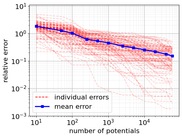
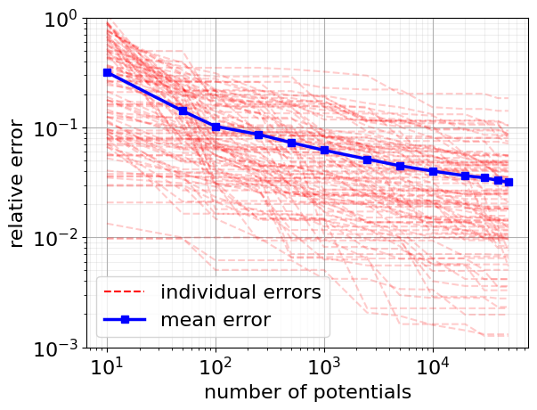
Figure 1. Experiment 6.1: Plot of the relative approximation error $\nicefrac{{\left(\operatorname{F}_{\vartheta}^{W^{2}_{2}}(\nu)-\operatorname{G}_{\vartheta}^{I_{j}}(\nu)\right)}}{{\operatorname{F}_{\vartheta}^{W^{2}_{2}}(\nu)}}$ for one hundred randomly drawn elements $\nu\in\mathcal{T}_{\mathrm{test}}$ and their mean against the number of potentials $j$. Left: MNIST. Right: CIFAR-10.