Variability of Blue Supergiants in the LMC with TESS

Abstract

The blue supergiant problem, namely the overabundance of blue supergiants (BSGs) inconsistent with classical stellar evolution theory, remains an open question in stellar astrophysics. Several theoretical explanations have been proposed, which may be tested by their predictions for the characteristic time variability. In this work, we analyze the light curves of a sample of 20 BSGs obtained from the Transiting Exoplanet Survey Satellite (TESS) mission. We report a characteristic signal in the low-frequency ($f\lesssim 2\,\mathrm{d}^{-1}$) range for all our targets. The power spectra has a peak frequency at $\sim 0.2\,\mathrm{d}^{-1}$, and we are able to fit it by a modified Lorentzian profile. The signal itself shows strong stochasticity across different TESS sectors, suggesting its driving mechanism happens on short ($\lesssim\mathrm{months}$) timescales. Our signals resemble those obtained for a limited sample of hotter OB stars and yellow supergiants, suggesting their possible common origins. We discuss three possible physical explanations: stellar winds launched by rotation, convection motions that reach the stellar surface, and waves from the deep stellar interior. The peak frequency of the signal favors processes related to convection caused by the iron opacity peak, and the shape of the spectra might be explained by the propagation of high-order, damped gravity waves. We discuss the uncertainties and limitations of all these scenarios.

1 Introduction

The formation pathways of blue supergiants (BSGs) are still not well understood. Despite being a unique class in the Hertzsprung-Russell (HR) diagram, their observed population disagrees with predictions from the classical theory of massive star evolution (Figure 1). Namely, if BSGs are massive single stars that have triggered hydrogen shell burning after central hydrogen depletion, their lifetime should be characterized by a thermal timescale on which their stellar envelope expands, typically $100-1000$ times faster than their main-sequence lifetime (Hoyle, 1960; Hofmeister et al., 1964). This means the occurrence rate of BSGs should be $100-1000$ times lower than massive main-sequence stars, clearly not consistent with their observed population (Castro et al., 2014, 2018; de Burgos et al., 2023). This discrepancy is known as the “blue supergiant problem,” and it remains one of the biggest open questions in the theory of stellar evolution (Bellinger et al., 2023).

Several alternative models for single stellar evolution have been proposed to solve the blue supergiant problem. Some authors argue that BSGs are actually central-helium burning stars with smaller cores, and typically longer lifetime. However, such theories usually require little or no mixing near the convective core boundary (Walborn et al., 1987; Weiss, 1989; Schootemeijer et al., 2019), a scenario disfavoured by our current-day knowledge of massive stars (Kaiser et al., 2020; Martinet et al., 2021). Some other authors argue that BSGs could be core-hydrogen burning stars that extend their main-sequences to cooler temperatures and larger luminosities, where most BSGs lie on the HR diagram (Kaiser et al., 2020). Such solutions typically require an excess amount of mixing beyond the convective core which produces large cores. They are the most satisfactory for hotter BSGs (Brott et al., 2011), but they appear to fail to match the very gradual observed decrease in the number of BSGs towards cooler temperatures (e.g.  Bellinger et al., 2023).

In addition to single stellar evolution pathways, it has been proposed that binary interactions may produce long-lived BSGs, motivated by the fact that a large fraction of young massive stars are found in binaries where close interactions or mergers may occur (Podsiadlowski et al., 1992; Kobulnicky & Fryer, 2007; Sana et al., 2012; de Mink et al., 2014). Interactions between two unevolved stars may produce rapidly rotating stars (de Mink et al., 2013), which may experience extra mixing resulting in an extended main sequence. If one of the stars has already evolved beyond the main sequence, it may give rise to a star with a smaller helium core compared to single stellar evolution products, either after accretion of hydrogen from a nearby star (Braun & Langer, 1995), or by merging with a hydrogen rich companion (Vanbeveren et al., 2013; Justham et al., 2014). Such a star could then evolve to a blue supergiant in the core-helium burning phase (Farrell et al., 2019). Finally, stars that are partially stripped may also spend some time in the BSG (Laplace et al., 2020; Klencki et al., 2020), although this effect seems to work best at low metallicity.

While it is uncertain which of these scenarios contribute to producing BSGs, they all concern different evolution pathways which are caused by some different stellar structure (especially core properties) compared to expectations from classical stellar evolution theory. As the structure of a star affects not only its lifetime, but also the energy transport processes from its interior to its surface, it is possible to introduce observational constraints by seeking time variability signals in BSGs. Specifically, Bellinger et al. (2023) argues that oscillations in the stellar interiors could provide unique asteroseismic signals which may help to distinguish different BSG formation scenarios.

In the past decades, several space missions have delivered high precision time series measurements for tens of thousands of stars, including CoRoT (Auvergne et al., 2009), Kepler/K2 (Borucki et al., 2010) and the Transiting Exoplanet Survey Satellite (TESS; Ricker et al. 2015). While a handful sample of BSG variability has been discovered with CoRoT and Kepler/K2 photometry (see, e.g., Aerts et al. 2010, 2017, 2018), the all-sky TESS mission offers a unique opportunity for a systematic study for BSGs due to its large field of view that covers hundreds of potential candidates. This motivates us to use TESS light curves to seek for photometric variability in BSGs.

In this work, we analyze the light curves of a sample of 20 BSGs in the Large Magellanic Cloud (LMC). We find a characteristic time variability signal in our sample that universally appears in LMC BSGs. The signal shows similarity to the low-frequency variability of other massive pulsators, suggesting they may have similar origins. The manuscript is organized as follows: we describe our sample selection procedure in Section 2 and present our results in Section 3. We compare our signals to low-frequency variability of other systems in Section 4, and in Section 5 we discuss the possible physical origins of our signal. We conclude in Section 6.

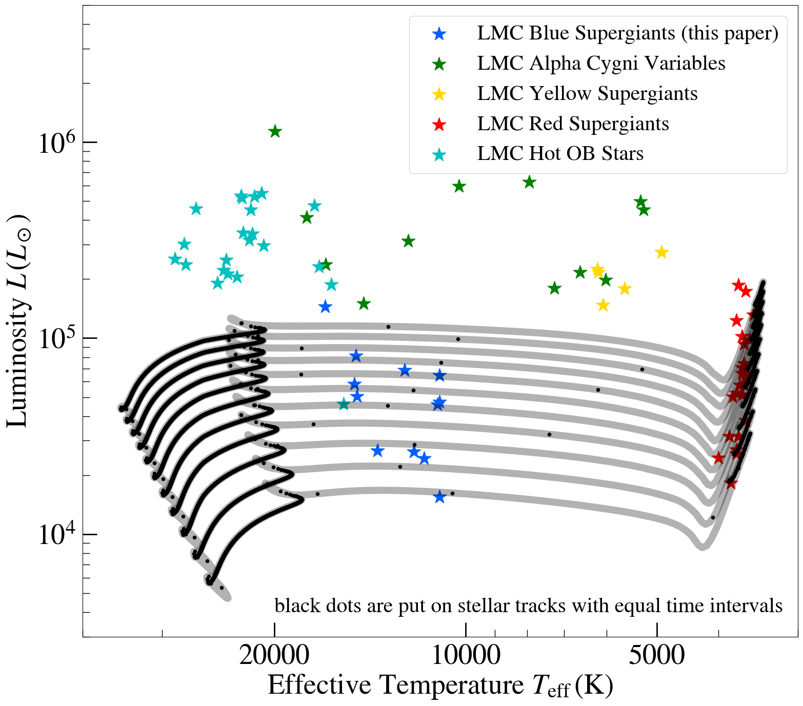
Figure 1: Blue supergiants (blue stars) form an extinct class in the Hertzsprung-Russel diagram, different from Alpha Cygni variables (green stars), yellow supergiants (yellow stars), red supergiants (red stars) or hot OB stars (cyan stars). When we put black dots with equal time intervals on the stellar tracks obtained from single stellar evolution model (from Bellinger et al. 2023), BSGs lie in the region where the number of dots are orders of magnitude less than the dots on the main-sequence, suggesting their occurrence rates should be orders of magnitude lower, inconsistent with the observed population. References: BSGs: 12 of the 20 stars in this paper with bolometric luminosity estimate; Alpha Cygnis: van Leeuwen et al. (1998); YSGs: Dorn-Wallenstein et al. (2020); RSGs: Neugent et al. (2020); hot OB Stars: from Bowman et al. (2019a) with bolometric luminosity estimate.

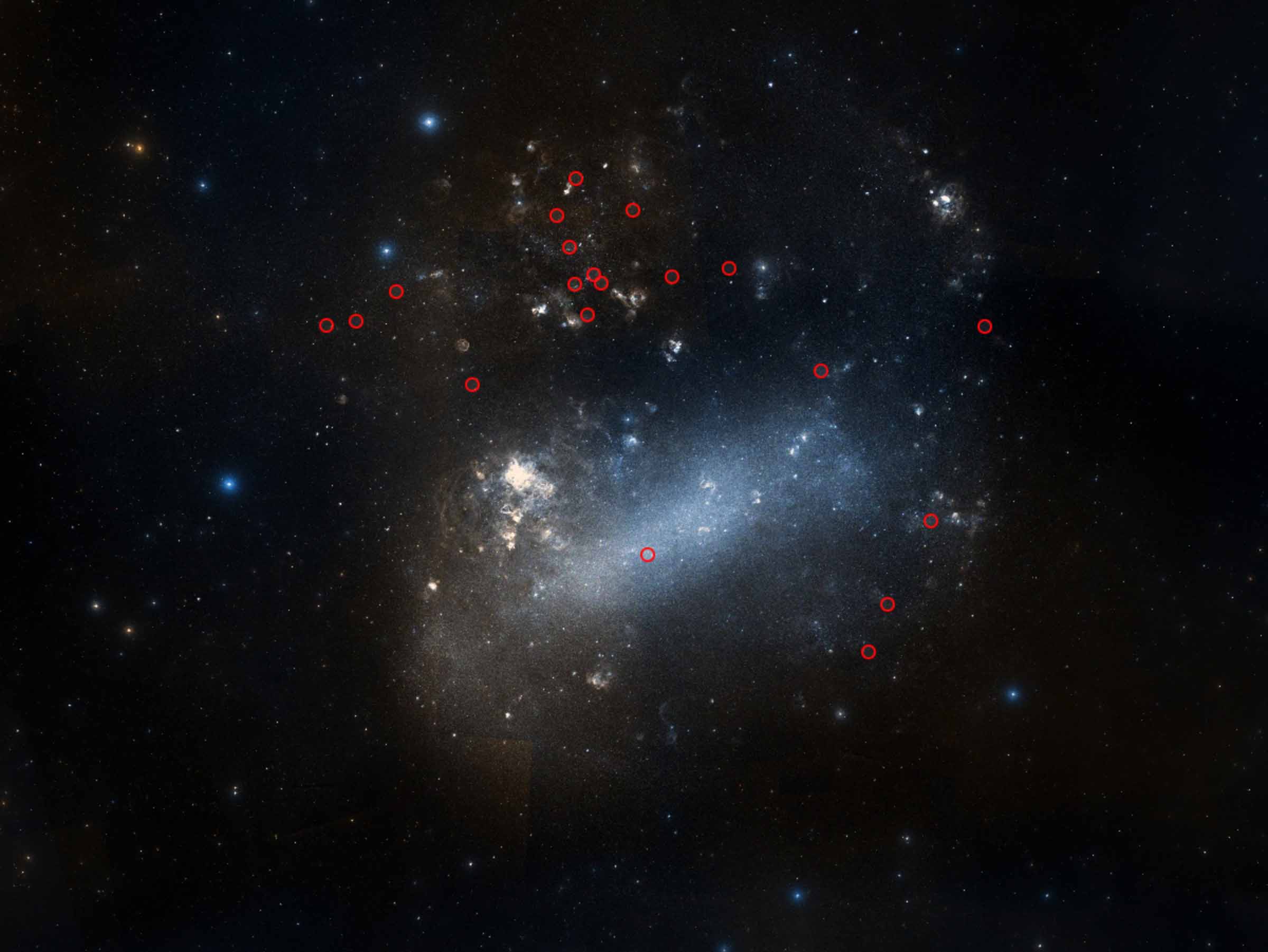
Figure 2: Locations of our BSG sample (red circles) in the Large Magellanic Cloud (obtained with DSS colored survey). Figure is made with SIMBAD (Wenger et al., 2000).

2 Sample Selection

Object Name	TIC Number	$T_{\mathrm{eff}}\;(\mathrm{K})$	$\log g\;(\mathrm{dex})$	$v\sin i\;(\mathrm{km/s})$	TESS Observing Sectors
SK -68 53	31179797	$13770\pm 740$	$2.09\pm 0.12$	$47.5\pm 11.5$	20 sectors: 27-31, 33, 34, 36-39, 61-69
SK -66 125	425086354	$14830\pm 760$	$2.34\pm 0.13$	$36.5\pm 11.5$	18 sectors: 27-35, 37-39, 62-64, 66-68
SK -67 283	31511729	$14880\pm 800$	$2.26\pm 0.14$	$46.5\pm 11.9$	12 sectors: 28, 29, 31, 32, 35, 38, 39, 61, 66-69
SK -69 31	30190076	$11830\pm 600$	$1.7\pm 0.12$	$44.0\pm 9.7$	20 sectors: 27-39, 61, 63-67, 69
SK -67 275	389864558	$14960\pm 890$	$2.23\pm 0.16$	$63.5\pm 12.1$	10 sectors: 27, 29, 30, 33, 36, 37, 39, 65, 68, 69
SK -66 142	276860494	$13640\pm 740$	$2.0\pm 0.12$	$49.0\pm 11.4$	19 sectors: 27, 28, 30-35, 37, 38, 61-69
HD 269639	287400996	$11000\pm 670$	$1.7\pm 0.15$	$26.5\pm 15.0$	19 sectors: 27, 28, 30, 31, 33-39, 61, 62, 64-69
SK -67 7	29987961	$12460\pm 760$	$1.83\pm 0.14$	$46.5\pm 11.8$	19 sectors: 27, 28, 30, 31, 33-39, 61-64, 66-69
SK -67 279	31311824	$11330\pm 600$	$1.9\pm 0.15$	$23.0\pm 10.2$	12 sectors: 29, 30, 32, 33, 35, 36, 38, 39, 61, 67-69
SK -70 31	30534618	$12060\pm 790$	$1.9\pm 0.15$	$33.0\pm 10.6$	21 sectors: 27-39, 61-63, 65-69
SK -68 152	389366376	$11000\pm 530$	$2.01\pm 0.13$	$34.0\pm 8.0$	16 sectors: 27, 29, 30, 32, 33, 35-39, 61, 64-66, 68, 69
SK -67 88	179638852	$11220\pm 600$	$1.78\pm 0.13$	$44.0\pm 10.0$	19 sectors: 27, 28, 30, 31, 33-39, 61, 62, 64-69
HD 269721	425084965	$11080\pm 600$	$1.7\pm 0.13$	$40.0\pm 8.9$	19 sectors: 27, 28, 30-38, 61, 62, 64-69
HD 269510	373682056	$11000\pm 620$	$1.7\pm 0.14$	$39.0\pm 10.6$	20 sectors: 27-30, 32, 33, 35-39, 61-69
SK -66 92	373845622	$13480\pm 750$	$1.92\pm 0.11$	$51.5\pm 11.0$	17 sectors: 27-35, 37, 38, 61, 62, 64, 66-68
SK -67 151	391809264	$11000\pm 510$	$2.24\pm 0.15$	$8.0\pm 19.8$	18 sectors: 27-31, 33, 34, 36-39, 61-63, 65-67, 69
SK -70 26	30403638	$11630\pm 570$	$1.9\pm 0.13$	$39.5\pm 9.8$	20 sectors: 27, 29-37, 39, 61-69
SK -67 171	425084139	$12650\pm 740$	$1.8\pm 0.12$	$47.5\pm 11.5$	16 sectors: 27, 28, 30, 31, 33, 34, 36-39, 61, 62, 65-67, 69
SK -67 133	287401176	$16630\pm 850$	$2.28\pm 0.12$	$53.5\pm 10.4$	29 sectors: 1, 3-11, 13, 27, 28, 30, 31, 33-39, 61, 62, 64-67, 69
SK -67 72	179038240	$12480\pm 750$	$1.84\pm 0.14$	$46.5\pm 11.8$	19 sectors: 27, 28, 30-38, 61-64, 66-69

Table 1: Names, Tess Input Catalog (TIC) numbers, spectroscopic data and TESS observing sectors of our BSG sample. $T_{\mathrm{eff}}$, $\log g$ and $v\sin i$ are taken from spectroscopic measurements from Serebriakova et al. (2023) (UVES preferred when measurements from both instruments available), where we quoted their $v\sin i_{\mathrm{SP}}$ for references.

We selected our sample from the 124 OB pulsators with spectroscopic measurements in Serebriakova et al. (2023), who obtained their data with the Ultraviolet and Visual Échelle Spectrograph (UVES; Dekker et al. 2000) and the Fiber-fed Extended Range Optical Spectrograph (FEROS; Kaufer et al. 1999) instruments attached to the UT2@VLT and MPG/ESO 2.2 m telescopes. Their sample is largely based on the massive stars in Bowman et al. (2019a) and Pedersen et al. (2019) with photometric variability detected in the first sector(s) of TESS data, and carried out high-resolution ($R\gtrsim 40000$), high-signal-to-noise-ratio ($S/N\sim 100$) two-epoch spectroscopy such that binaries were excluded. The targets all locate in the Southern Continuous Viewing Zone (CVZ-S) of TESS and its vicinity, with high-duty-cycle photometric data of between approximately 200 days and 1 year in duration.

Out of the 148 pulsators, we selected 41 BSG candidates on the spectroscopic HR diagram, with $3.2<\log{(\mathcal{L}/\mathcal{L}_{\odot}})<4.0$ and $T_{\mathrm{eff}}<30000\,\mathrm{K}$, where $\mathcal{L}:=T_{\mathrm{eff}}^{4}/g$ is the spectroscopic luminosity (Langer & Kudritzki, 2014). The more luminous stars may still be BSGs of higher masses, yet we exclude them from our candidates since their evolution stages are even less clear (see Section 4 for a comparison between our sample and a limited sample of hotter B stars). Bolometric corrections turn out to be difficult for these candidates since many of them do not have reliable measurements of extinction, hence we did not select our sample from their real luminosities.

As each TESS pixel has an angular size of $21^{\prime\prime}$, stars around our targets could cause contamination to the light curve, and this is especially an issue when the star locates in crowded regions of the sky (Pedersen & Bell, 2023). To exclude false signals caused by nearby stars, we used the LATTE package (Eisner et al., 2020) to obtain star fields for all our candidates from both TESS and Gaia Data Release 2 (Gaia Collaboration et al., 2018). We compared the star fields and only kept the candidates without any bright (defined by the difference of magnitudes $\Delta m<4$) neighbours in the same TESS pixel as them. After such treatment 20 stars are left in our final sample. It turns out that they are all in the LMC (Figure 2), and their spectroscopic properties are listed in Table 1.

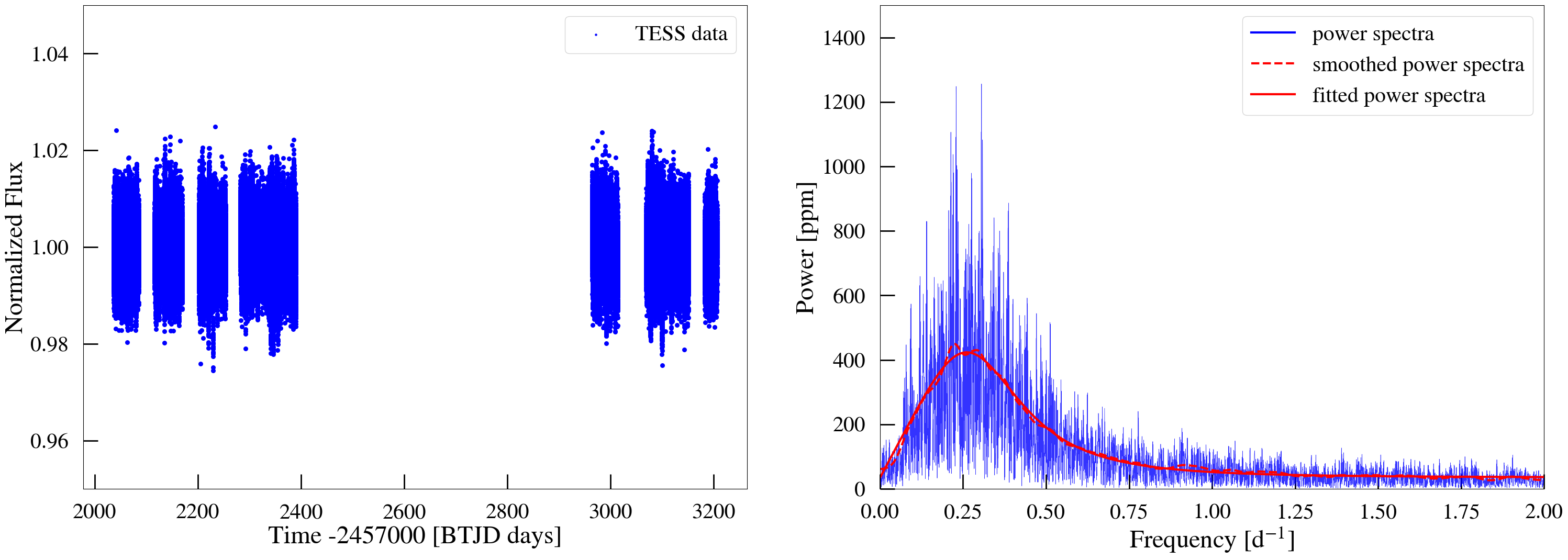
Figure 3: TESS data and power density spectra of SK -67 171 (TIC425084139). The smoothed and fitted spectrum are shown in dashed and solid red lines. The power density spectrum shows a pattern with a peak frequency at $\sim 0.25\,\mathrm{d}^{-1}$, and can be fitted by a modified Lorentzian profile (see main text).

We used the Python package Lightkurve (Lightkurve Collaboration et al., 2018) to pull TESS light curve data for our sample, using the data processed by a pipeline developed by the Science Processing Operations Center (SPOC; Jenkins et al. 2016). We used Astropy to analyze the data (Astropy Collaboration et al., 2013, 2018, 2022). Our sample have 10-29 observing sectors available from TESS, with typical observation period of $\sim 3$ years (sector 27-69, from July 5, 2020 to September 30, 2023). Their details are summarized in Table 1.

3 Results

Here we present our results of identifying and characterising the variability for the BSGs in our study.

3.1 Universal Signal in BSGs

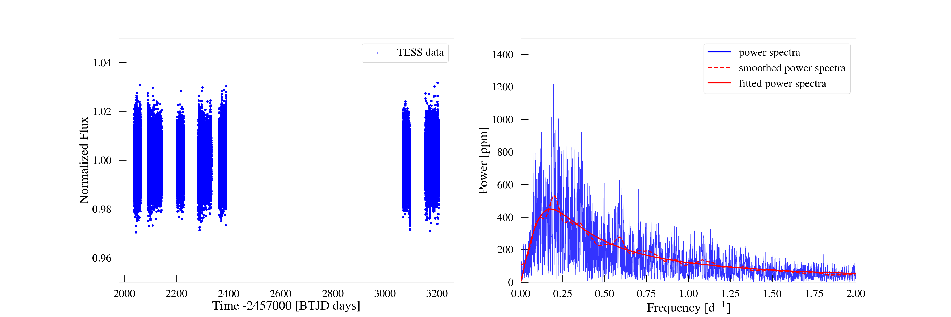
Figure 13: TESS data and power density spectra of SK -67 275 (TIC389864558). The smoothed and fitted spectrum are shown in dashed and solid red lines.

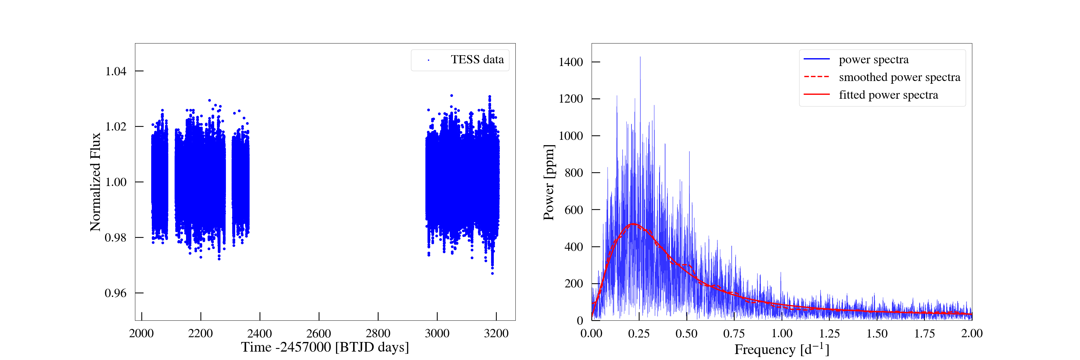
Figure 14: TESS data and power density spectra of SK -66 142 (TIC276860494). The smoothed and fitted spectrum are shown in dashed and solid red lines.

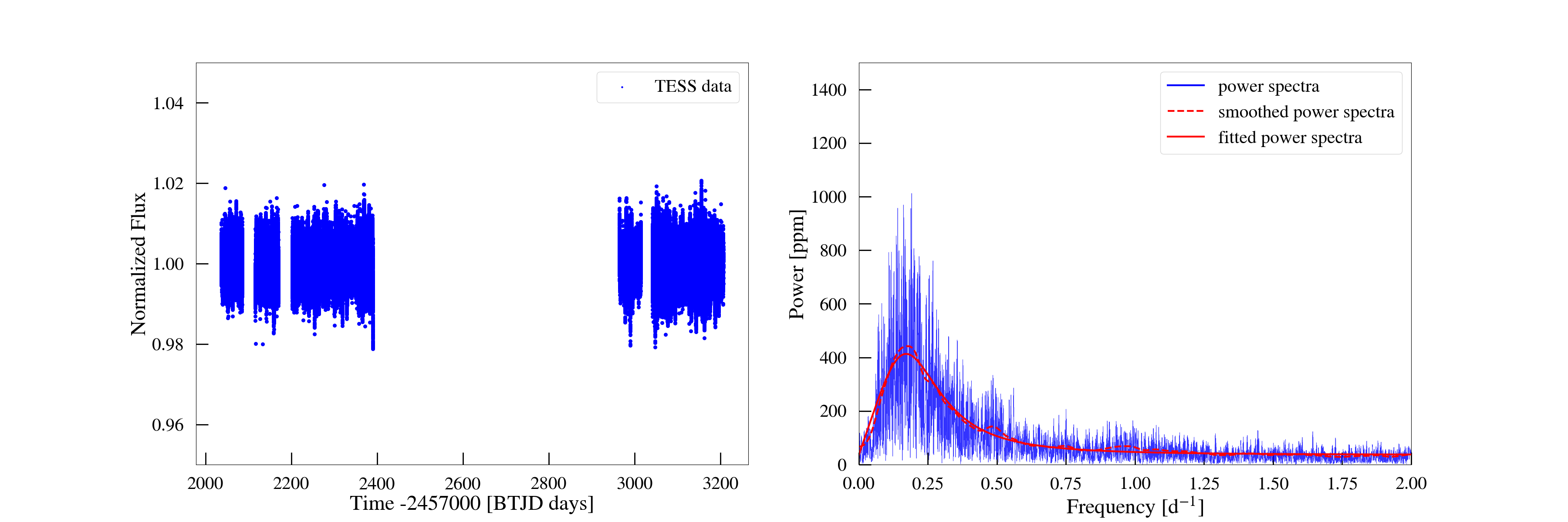
Figure 15: TESS data and power density spectra of HD 269639 (TIC287400996). The smoothed and fitted spectrum are shown in dashed and solid red lines.

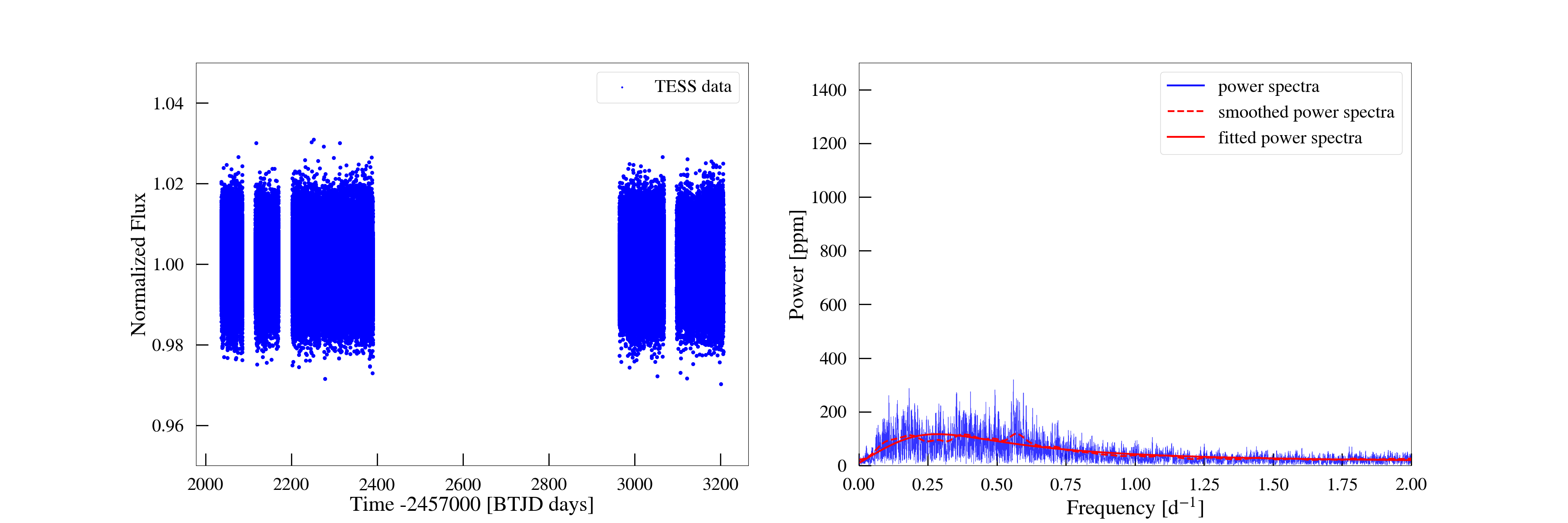
Figure 16: TESS data and power density spectra of SK -67 7 (TIC29987961). The smoothed and fitted spectrum are shown in dashed and solid red lines.

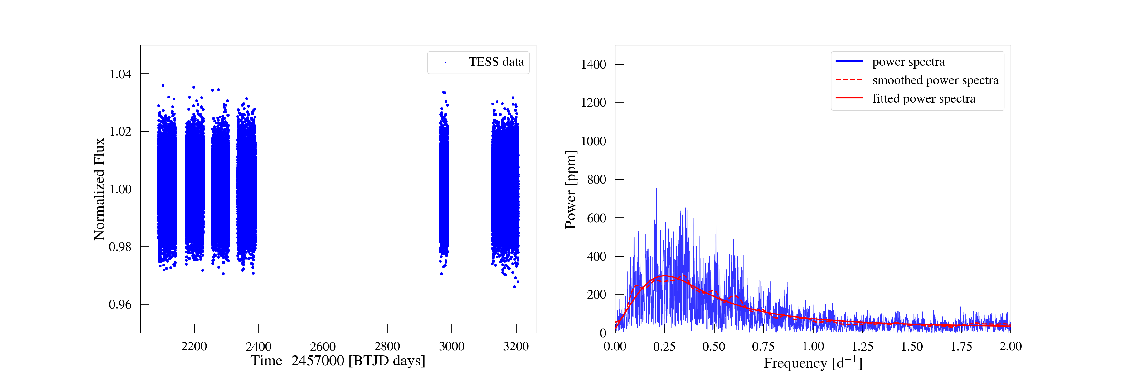
Figure 17: TESS data and power density spectra of SK -67 279 (TIC31311824). The smoothed and fitted spectrum are shown in dashed and solid red lines.

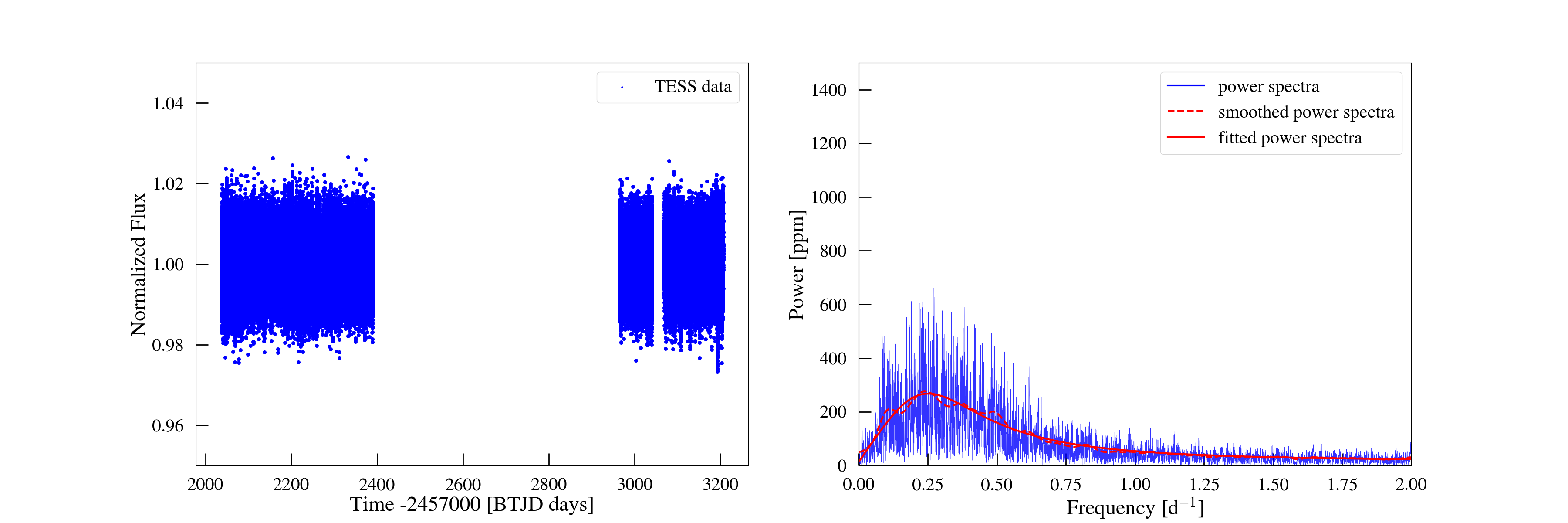
Figure 18: TESS data and power density spectra of SK -70 31 (TIC30534618). The smoothed and fitted spectrum are shown in dashed and solid red lines.

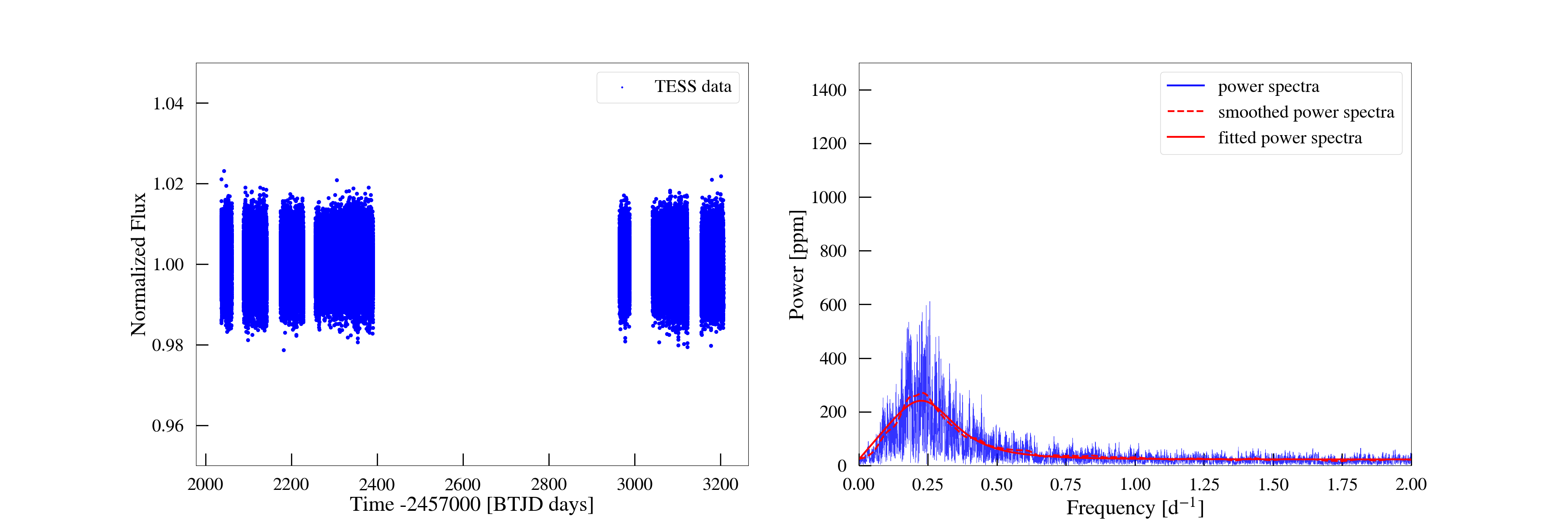
Figure 19: TESS data and power density spectra of SK -68 152 (TIC389366376). The smoothed and fitted spectrum are shown in dashed and solid red lines.

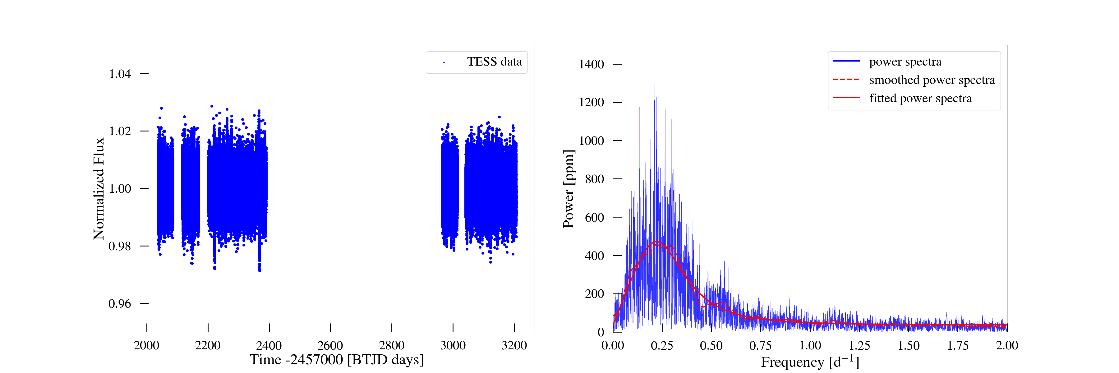
Figure 20: TESS data and power density spectra of SK -67 88 (TIC179638852). The smoothed and fitted spectrum are shown in dashed and solid red lines.

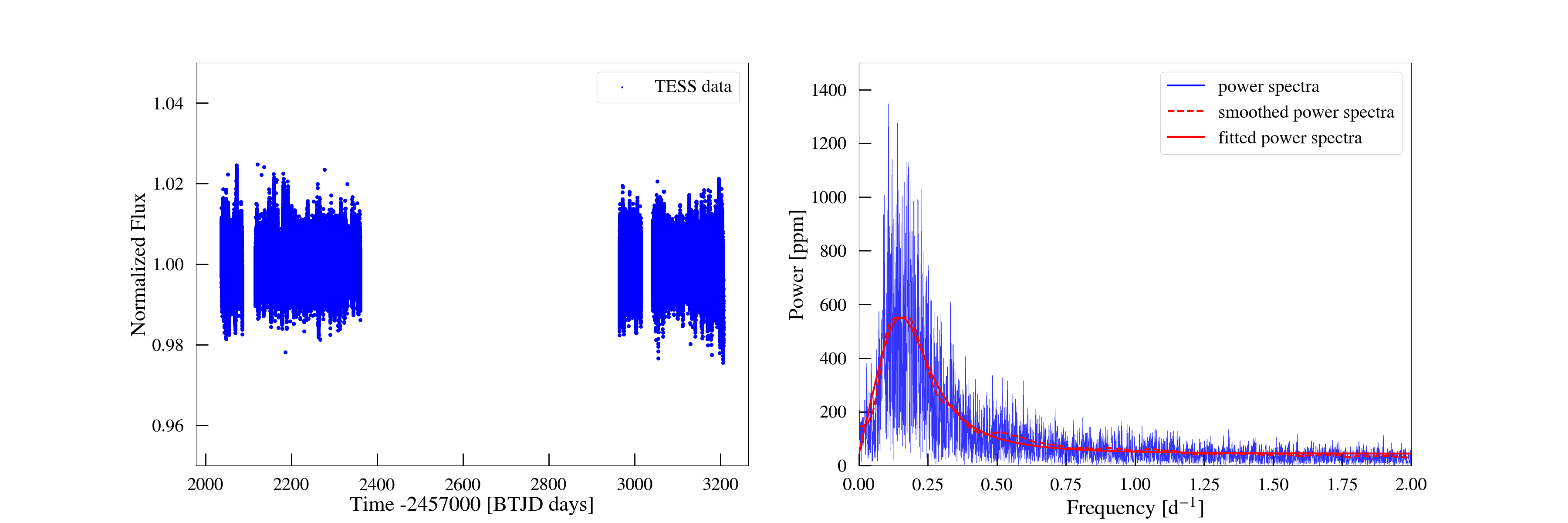
Figure 21: TESS data and power density spectra of HD 269721 (TIC425084965). The smoothed and fitted spectrum are shown in dashed and solid red lines.

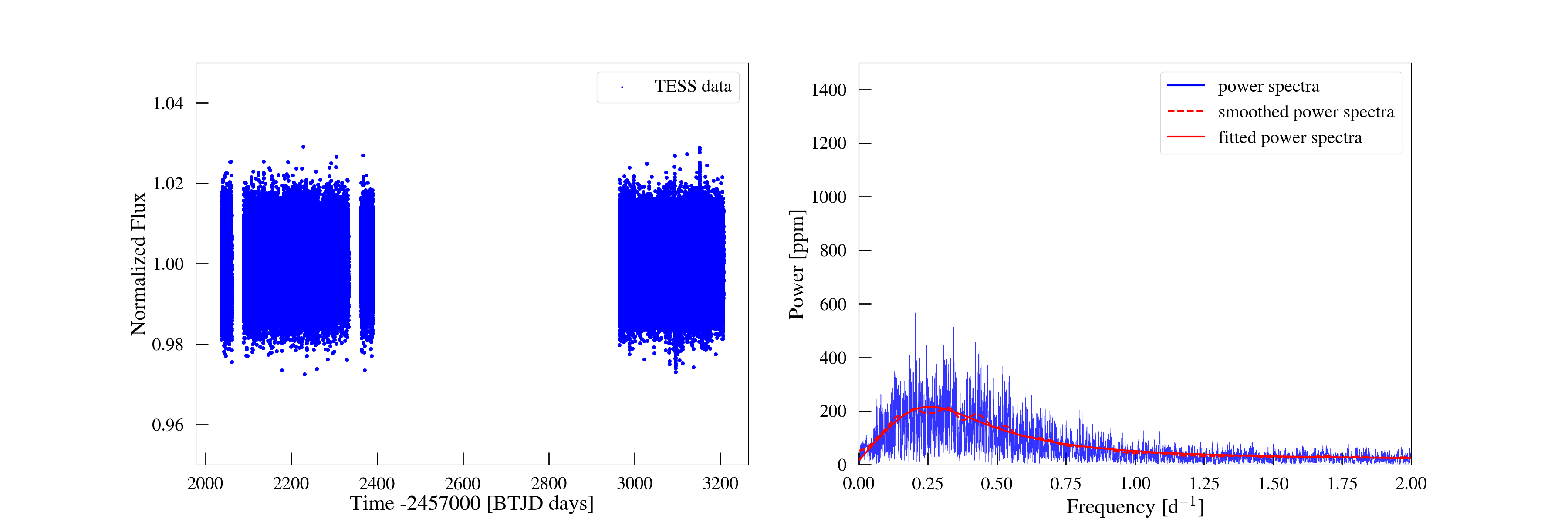
Figure 25: TESS data and power density spectra of SK -70 26 (TIC30403638). The smoothed and fitted spectrum are shown in dashed and solid red lines.

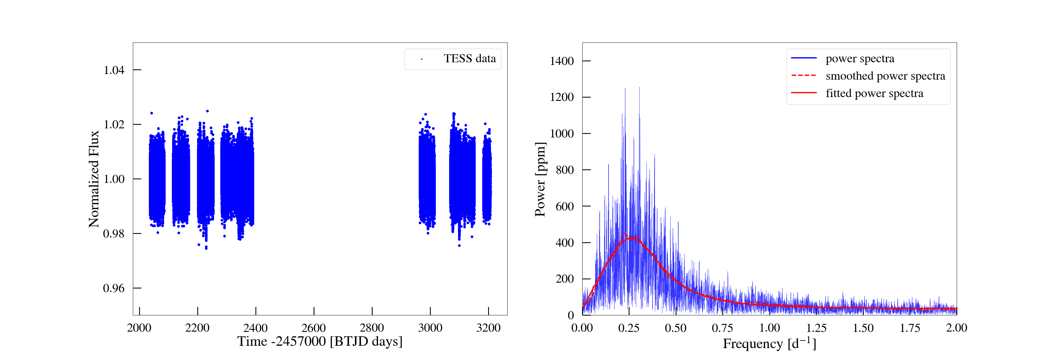
Figure 26: TESS data and power density spectra of SK -67 171 (TIC425084139). The smoothed and fitted spectrum are shown in dashed and solid red lines.

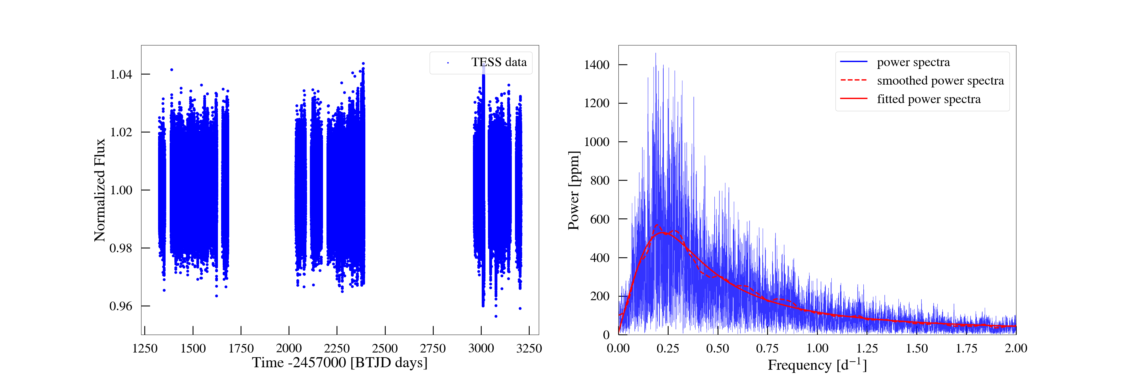
Figure 27: TESS data and power density spectra of SK -67 133 (TIC287401176). The smoothed and fitted spectrum are shown in dashed and solid red lines.

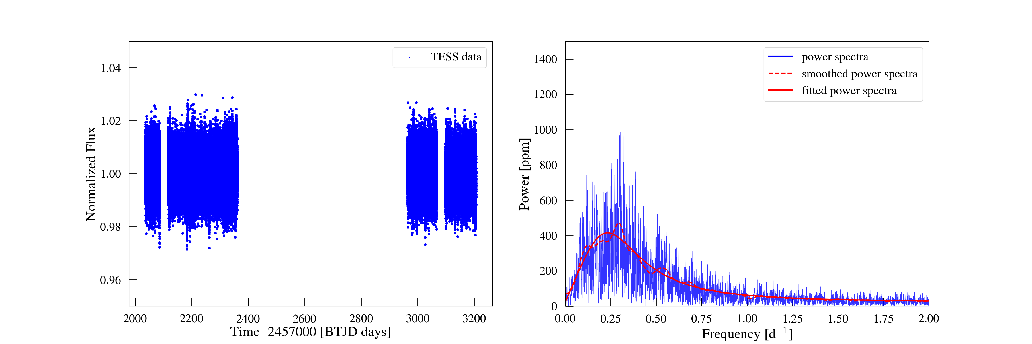
Figure 28: TESS data and power density spectra of SK -67 72 (TIC179038240). The smoothed and fitted spectrum are shown in dashed and solid red lines.

Figure 3 shows the TESS data and periodogram of one typical example system in our sample: SK -67 171 (TIC425084139). The results for all our sample can be seen from Figures 9-28 in the Appendix. While we do not see any significant individual modes from the periodogram of this particular system, we do identify a low-frequency ($f<2\,\mathrm{d}^{-1}$) variability signal from the Fourier transform of the time series, as shown. The signal goes to zero power towards high and low frequencies, with a characteristic peak frequency at $\sim 0.25\,\mathrm{d}^{-1}$. We see in the Appendix that this signal appears in all of the targets in our sample, suggesting it may be a ubiquitous phenomenon.

The high-frequency tail above the peak frequency in our signal looks very similar to a characteristic signal that has already been widely discussed in hot massive stars, commonly referred as the stochastic low-frequency (SLF) variability or “red noise” (Bowman et al., 2019a, b, 2020; Bowman & Dorn-Wallenstein, 2022; Dorn-Wallenstein et al., 2022; Szewczuk et al., 2021). We note that, however, the signal patternin our sample is distinct as it has decaying power towards zero frequency, while the red noise signal mostly concerns the high frequency tail. As the red noise signal is usually fitted with a super Lorentzian profile (e.g., Kallinger et al. 2014), we are motivated to characterize our power density spectra with the following modified Lorentzian profile:

$$P(\nu)=W_{0}+\alpha_{0}\frac{(\nu/\nu_{\mathrm{char}})}{1+(\nu/\nu_{\mathrm{char}})^{\gamma}}\,,$$ (1)

which is a linear profile times a super-Lorentzian profile with three parameters ($\nu_{\mathrm{char}}$, $\alpha_{0}$ and $\gamma$), plus a background noise term $W_{0}$. This profile captures the shape of the signal with a peak frequency $\nu_{\mathrm{peak}}=(\gamma-1)^{-1/\gamma}\nu_{\mathrm{char}}$ and a tendency towards zero at both high and low frequencies. It also resembles the high frequency tail of super-Lorentzian profile above the peak frequency.

We smoothed our power spectra with a window size of $0.1\,\mathrm{d}^{-1}$ and fitted the smoothed spectra with the above function using a non-linear least squares method with the curve_fit function in the Python package ScipPy (Virtanen et al., 2020). The fitting parameters we found are shown in Table 2 and an example fitting curve is shown in Figure 3 (for all other stars in our sample, see Figures 9-28). We found that our fitting profile matches the smoothed spectrum very well, with the background-noise term $W_{0}$ at least one order-of-magnitude lower than the characteristic power term $\alpha_{0}$. The physical peak frequency $\nu_{\mathrm{peak}}$ is around $0.2$ days, and the power-law index $\gamma$ ranges from $2$ to $5$, revealing a universal pattern in all our stars with small dispersion. We note that, however, the profile is not physically motivated and we did not find any strong correlations between the fitting parameters and the spectroscopic properties of our sample, which may give insights to the physical origins of the signal. We confirmed that our fitting parameters are robust against tests with different choices of smoothing windows sizes.

3.2 Time Variability of the Signal

Object	$W_{0}$	$\alpha_{0}$	$\nu_{\mathrm{char}}\;$	$\gamma$	$\nu_{\mathrm{peak}}$
	(ppm)	(ppm)	$(\mathrm{d}^{-1})$		$(\mathrm{d}^{-1})$
SK -68 53	7.0	864.67	0.235	2.6	0.195
SK -66 125	27.1	727.40	0.256	2.8	0.209
SK -67 283	10.5	1108.24	0.184	2.3	0.164
SK -69 31	47.7	1021.72	0.236	4.1	0.179
SK -67 275	1.6	889.66	0.195	2.2	0.178
SK -66 142	17.2	953.07	0.277	3.0	0.219
HD 269639	36.2	672.25	0.224	3.8	0.171
SK -67 7	9.0	208.45	0.344	2.7	0.284
SK -67 279	20.9	524.19	0.315	3.0	0.251
SK -70 31	14.3	472.39	0.321	3.2	0.251
SK -68 152	22.5	358.37	0.298	5.1	0.226
SK -67 88	35.6	749.95	0.292	4.3	0.221
HD 269721	43.3	896.16	0.200	3.9	0.152
HD 269510	16.0	331.78	0.117	2.5	0.099
SK -66 92	30.0	1143.31	0.277	3.4	0.214
SK -67 151	25.2	299.23	0.298	4.8	0.226
SK -70 26	15.8	375.17	0.325	3.1	0.256
SK -67 171	35.0	662.57	0.345	4.4	0.261
SK -67 133	9.4	1004.97	0.271	2.7	0.223
SK -67 72	21.8	721.37	0.301	3.4	0.233

Table 2: Fitting parameters and the physical peak frequency $\nu_{\mathrm{peak}}=(\gamma-1)^{-1/\gamma}\nu_{\mathrm{char}}$ for the modified Lorentzian profile (Equation 1) that best matches our signal.

The above analysis was carried out with the full TESS data obtained for our BSG sample, across multiple sectors. With an average observing time of 27 days per sector, the full TESS light curve gives us a frequency resolution of $0.001-0.005$ d^-1. We note that, however, the signal actually varies in time as well, as seen by analysing each observed sector individually.

Figure 4 shows the power spectrum obtained from individual sectors for the example BSG SK -67 171. Each bar represents a power spectra from one sector, with the color mapping the power at different frequencies (such that a “lighter” color region represents a peak at that frequency). The full power spectra combining all sectors is shown in the bottom for reference. We see that the shape of the power spectrum for individual sectors are different from each other and the full power spectra. Some features in one sector is preserved in the next sector (e.g., in sectors 27 and 28), while some only comes back after a few sectors (e.g., in sectors 33 and 36), or never repeats. We note that as the frequency resolution of individual sector is as low as $\Delta f\sim 1/27\,\mathrm{d}=0.04\,\mathrm{d}^{-1}$, we cannot identify any of the features as distinct modes excited. Nevertheless, we found similar variability of the features for all our sample.

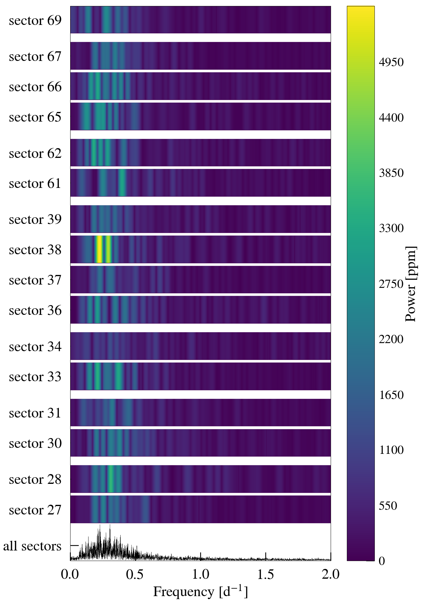
Figure 4: The power spectrum from individual TESS sectors for BSG SK -67 171. Each bar represents a power spectra from one sector, with the color mapping the power at different frequencies (such that a “lighter” color region represents a peak at that frequency). The full power spectra combining all sectors is shown in the bottom for reference. We see clear time variability of the spectra across different sectors.

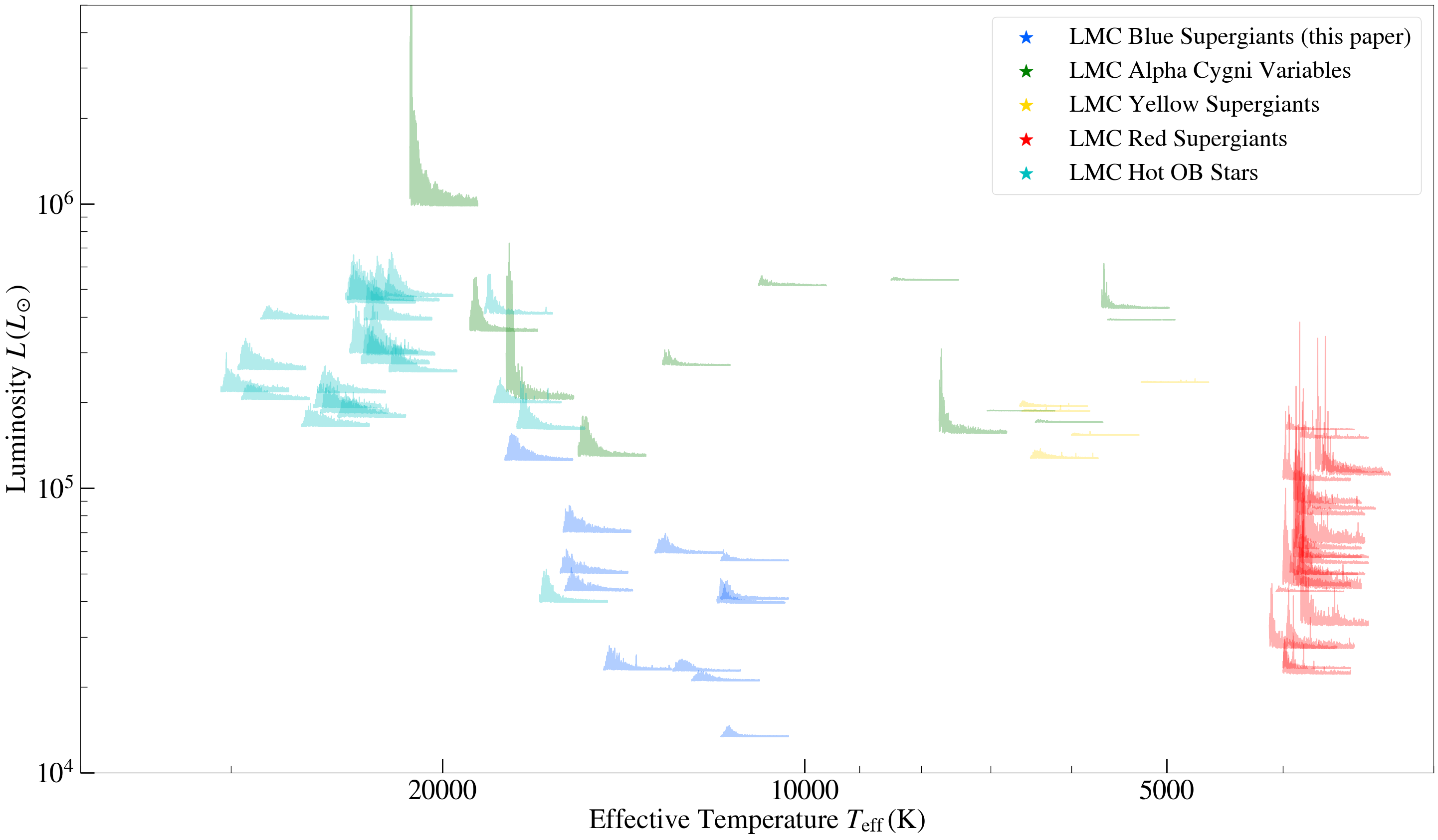
Figure 5: The power spectra of 12 BSGs in the $0-2\,\mathrm{d}^{-1}$ frequency range plotted on their locations on the HR diagram, compared to other types of stars (see Figure 1). We see similar kind of variability in hotter OB stars and around half of the Alpha Cygni variables, suggesting they may share similar origins. References: BSGs: 12 of the 20 BSG in this paper with bolometric luminosity estimate; Alpha Cygnis: van Leeuwen et al. (1998); YSGs: Dorn-Wallenstein et al. (2020); RSGs: Neugent et al. (2020); hot OB Stars: 22 stars from Bowman et al. (2019a) with bolometric luminosity estimate and spectroscopy measurements from Serebriakova et al. (2023).

Object	$T_{\mathrm{eff,spec}}\;(\mathrm{K})$	$\log(L_{\mathrm{bol}}/L_{\odot})$	$R_{\mathrm{bol}}/R_{\odot}$	$\nu_{\mathrm{peak}}\;(\mathrm{d}^{-1})$	$v_{\mathrm{eq,derive}}$ (km/s)	$v\sin i$ (km/s)	$(\sin i)_{\mathrm{derive}}$
SK -68 53	13770	4.425	28.7	0.195	283.4	47.5	0.17
SK -66 125	14830	4.703	34.0	0.209	359.2	36.5	0.10
SK -67 283	14880	4.909	42.8	0.164	354.9	46.5	0.13
SK -67 275	14960	4.765	35.9	0.178	323.7	63.5	0.20
HD 269639	11000	4.674	59.8	0.171	518.5	26.5	0.05
SK -70 31	12060	4.421	37.2	0.251	472.9	33.0	0.07
SK -68 152	11000	4.191	34.3	0.226	392.7	34.0	0.09
HD 269721	11080	4.660	58.0	0.152	447.0	40.0	0.09
HD 269510	11000	4.809	69.9	0.099	351.7	39.0	0.11
SK -70 26	11630	4.387	38.5	0.256	498.0	39.5	0.08
SK -67 133	16630	5.162	45.9	0.223	517.4	53.5	0.10
SK -67 72	12480	4.836	56.0	0.233	660.1	46.5	0.07

Table 3: The derived bolometric luminosity, radius and equatorial velocity of 12 BSGs in our sample. The derived equatorial velocities are not compatible with spectroscopic $v\sin i$ measurements, typically one order of magnitude too large.

As each TESS sector only observes for a period of $\sim 27\,\mathrm{days}$, such time variability in our signal suggests that the physical mechanism related to them must be very short, occurring on timescales shorter than $\sim$ 30 days. If the signal is stochastically excited from the stellar interior (see discussions in 5.3), the driving mechanisms must happen on such short timescales as well, and the characteristic signals they excite must be at least equally short-lived. This put additional constraints on understanding the physics behind them.

4 Comparison to Low-Frequency Variability in Other LMC Stars

Low-frequency photometric variability has been found and discussed in different kinds of massive stars on the HR diagram, including hot OB stars (Bowman et al., 2019b) and evolved yellow supergiants (Dorn-Wallenstein et al., 2019, 2020). To look for their similarities and possible common physical origins, we analyse a limited sample of other LMC stars and compare them with our BSG sample.

In Figure 5 we show the periodograms (between $0-2\,\mathrm{d}^{-1}$) for various types of stars with their positions on the HR diagram. This includes 12 BSGs from this study with bolometric luminosity estimates (listed in Table 3), 5 yellow supergiants from Dorn-Wallenstein et al. (2020), 23 red supergiants from Neugent et al. (2020), 12 alpha Cygni variables from van Leeuwen et al. (1998) and 22 hot OB stars from the TESS OB sample in Bowman et al. (2019b) with bolometric luminosity estimates and spectroscopy measurements from Serebriakova et al. (2023). The data are acquired with TESS with similar analysis as described in 2. With this limited sample, we clearly see similarities between the variability of hot OB stars and our BSG sample. Some of the alpha Cygni variables and yellow supergiants resemble the the signal we found in BSGs, yet with much lower power, while some other alpha Cygni variables show a massive peak at very low frequency with no clear turnover. The red supergiants, on the hand, form the most distinct class on the HR diagram and typically show some multi-peaks pattern in the periodogram, very different from BSGs.

Previous photometric analysis on OB stars and yellow supergiants mostly interpret the low-frequency variability as “red noise”, characterized by some function that levels off at zero frequency (Bowman et al., 2019b; Dorn-Wallenstein et al., 2019, 2020), which is clearly not what we see. This is probably because these authors mostly carry out their time-series analysis for light curves shorter than $\lesssim 100\,\mathrm{days}$, such that the characteristic low-frequency turnover cannot be well resolved in Fourier space. Nevertheless, the existing theoretical explanations for their signals are still relevant to our sample, given the similarities between these signals, which is what we probe in the next section.

5 Discussions

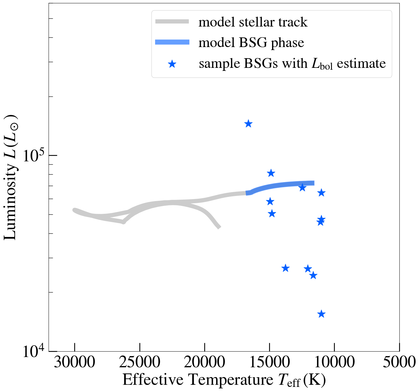
Figure 6: The stellar track of a $15\,M_{\odot}$ BSG model with a metallicity of $0.008$ on the HR diagram. This is a central helium burning star formed after a stellar merger (Bellinger et al., 2023), with a BSG lifetime of 1 Myr (highlighted with thick blue line). The positions of 12 BSGs with derived bolometric luminosities in our sample are shown as blue stars.

In this section we discuss the possible physical mechanisms that may cause the signal we found in our BSG sample and assess their viability in explaining the signal that we discuss in this work.

5.1 Stellar Winds

It is believed that stellar winds launched from the surface may cause low-frequency variability in massive stars. These clumpy and inhomogeneous winds are caused by some radiative driving mechanism whose exact details are still under debate (Owocki & Rybicki, 1984; Puls et al., 1996, 2006, 2008). They might be responsible for the “red noise” signal (see, e.g., Aerts et al. 2018; Ramiaramanantsoa et al. 2018; Krtička & Feldmeier 2018, 2021) or even the large macroturbulence observed in spectroscopy of massive stars (e.g., Simón-Díaz et al. 2017).

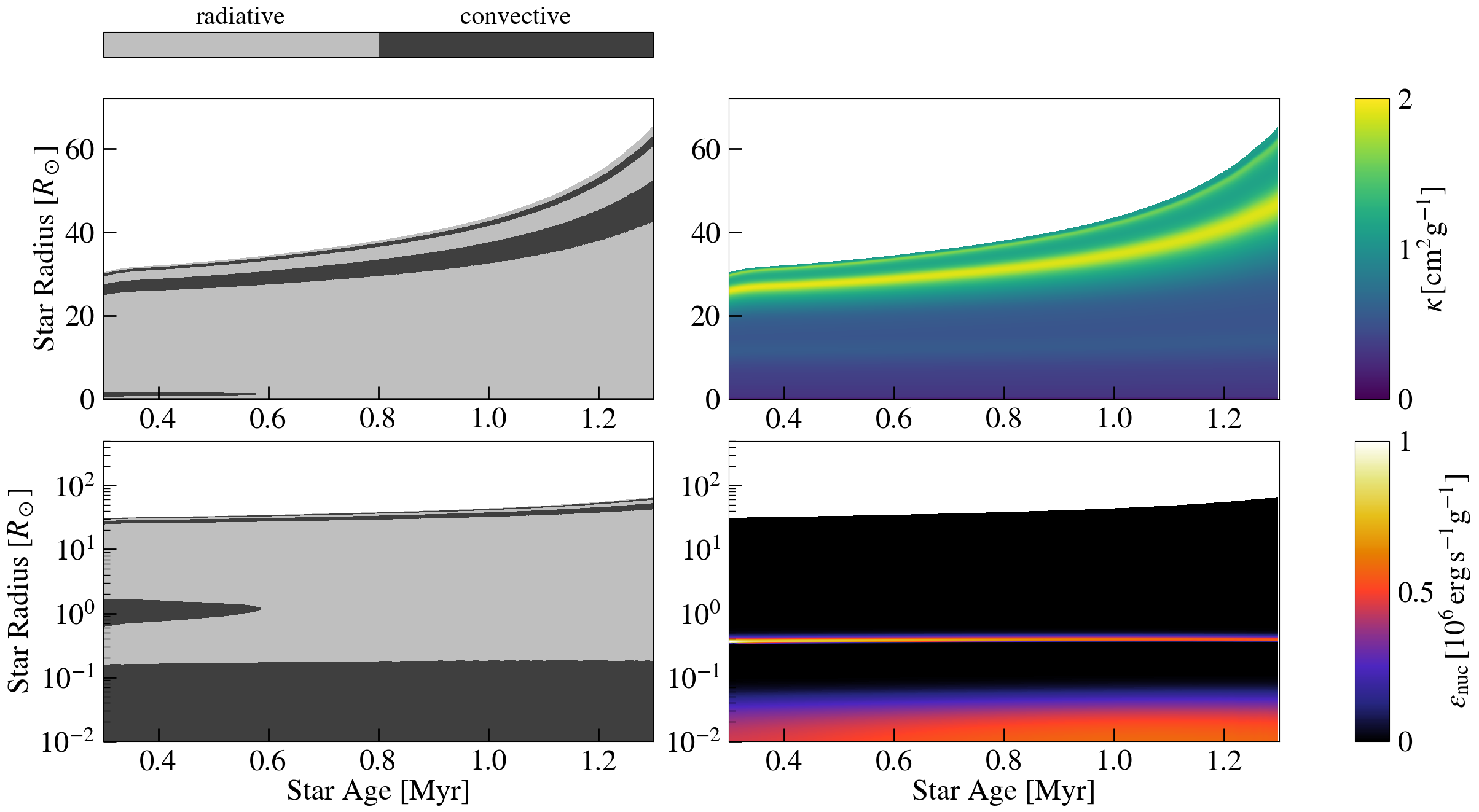
Figure 7: The stellar structure upon radius of our $15\,M_{\odot}$ model throughout its evolution in the BSG phase (thick blue line in Figure 6). The upper panels are in linear coordinates and the lower panels are in logarithm to make the core structures easier to see. Left: zone types of the star. We see two subsurface convective zones and a convective core. Before 0.6 Myr there is also a convective zone above the shell-burning region; Right: the opacity and nuclear generation rate of the model. The opacity profile shows two major peaks corresponding to the subsurface convective zones, and nuclear energy indicates that the two additional convective regions are caused by shell and core burning.

Blomme et al. (2011) argues that if stellar winds cause some low-frequency signal, its frequency should be compatible to the stellar rotation frequency at which the winds are launched, and one can then compare the equatorial velocity $v_{\mathrm{eq,derive}}:=2\pi\nu_{\mathrm{peak}}R_{\mathrm{star}}$ derived from the peak frequency of the signal with spectroscopic $v\sin i$ measurements of the star. To test this scenario, we derive the bolometric luminosity $L_{\mathrm{bol}}$ of 12 BSGs in our sample with reliable G-band magnitude and extinction measurements from Gaia (Gaia Collaboration et al., 2018, 2023), with the bolometric correction table provided by the Mesa Isochrones and Stellar Tracks (MIST) grids (Dotter, 2016; Choi et al., 2016), assuming a distance of 49.97 kpc (the distance of LMC). We then derived their radii $R_{\mathrm{bol}}$ with the spectroscopic $T_{\mathrm{eff}}$ from Serebriakova et al. (2023), and calculated their derived equatorial velocities based on the fitted characteristic frequency in the signal. The results are shown in Table 3. Despite the uncertainties we introduced in this process, we found that $v_{\mathrm{eq,derive}}$ for these stars are generally one order of magnitude larger than their measured $v\sin i$, suggesting their inclinations are all less than $\sim 10$ degrees. Hence we do not believe the signal is likely caused by stellar winds.

We note, however, whether $v\sin i$ measurements from spectroscopy should be interpreted as stellar rotation is actually unclear. For example, Simón-Díaz & Herrero (2014) and Simón-Díaz et al. (2017) point out that macroturbulent velocities may contribute to the total broadening of spectral lines in OB stars at least as equally as rotation, such that the measured $v\sin i$ overestimates the real stellar rotation rate (Schultz et al., 2023b). Nevertheless, this picture only disproves the wind scenario more since it predicts even lower peak frequency, compared to what we found from the signal.

5.2 Subsurface Convection

Historically, stochastic and non-periodic variability is mostly discussed in solar-like oscillators and red giants, in the context of its association with surface convection and granulation (Schwarzschild, 1975; Michel et al., 2008; Chaplin & Miglio, 2013; Kallinger et al., 2014; Hekker & Christensen-Dalsgaard, 2017). In massive stars, subsurface convective zones caused by opacity peaks associated with iron and helium ionization may create convective motion in the stellar photosphere, observed as low-frequency photometric variability (Cantiello et al., 2009b, 2021).

To see if these subsurface convective zones are related to our signal, we looked into a $15\,M_{\odot}$ BSG model from Bellinger et al. (2023) with a metallicity of 0.008 (a typical value for LMC stars), made with the Modules for Experiments in Stellar Astrophysics (MESA r23.05.1, Paxton et al. 2011, 2013, 2015, 2018, 2019; Jermyn et al. 2023). The model starts as a post-merger star with a helium core and a hydrogen envelope, and it evolves to a BSG during its central helium burning phase, with a BSG lifetime of 1 Myr (see Figure 6 for a comparison between the model and our sample on the HR diagram). While some authors argue that single stellar evolution could also produce BSGs (see, e.g., Walborn et al. 1987; Weiss 1989; Schootemeijer et al. 2019; Kaiser et al. 2020), the BSG sub-surface structures should be similar in those alternative models, since the occurrence of element opacity peaks is most determined by temperature.

In Figure 7 we show the structure (zone types, opacity and nuclear burning rates) of our model throughout the BSG phase. We see two subsurface convective zones corresponding to the opacity peaks caused by helium and iron ionization, at $\log(T)=4.7$ and $5.3$. We note, however, the subsurface convective zones in our model are much deeper than those found from Cantiello et al. (2009b), who mostly concerned less evolved main-sequence stars. Our convective zones are typically $\gtrsim 0.5\,R_{\odot}$ below the stellar photosphere, one order of magnitude deeper than their findings (see Figure 2 in Cantiello et al. 2009b for comparison). This means subsurface convection is less likely to be observed as photosphere variability for BSGs. Nevertheless, as we used mixing length theory (MLT) to treat convection in our 1D stellar evolution model, we may seriously underestimate the spatial extension of convection, as confirmed in some recent 3D simulations on subsurface convection (Schultz et al., 2022, 2023a, 2023b). In reality the subsurface convective zones may extend to the surface to be observed.

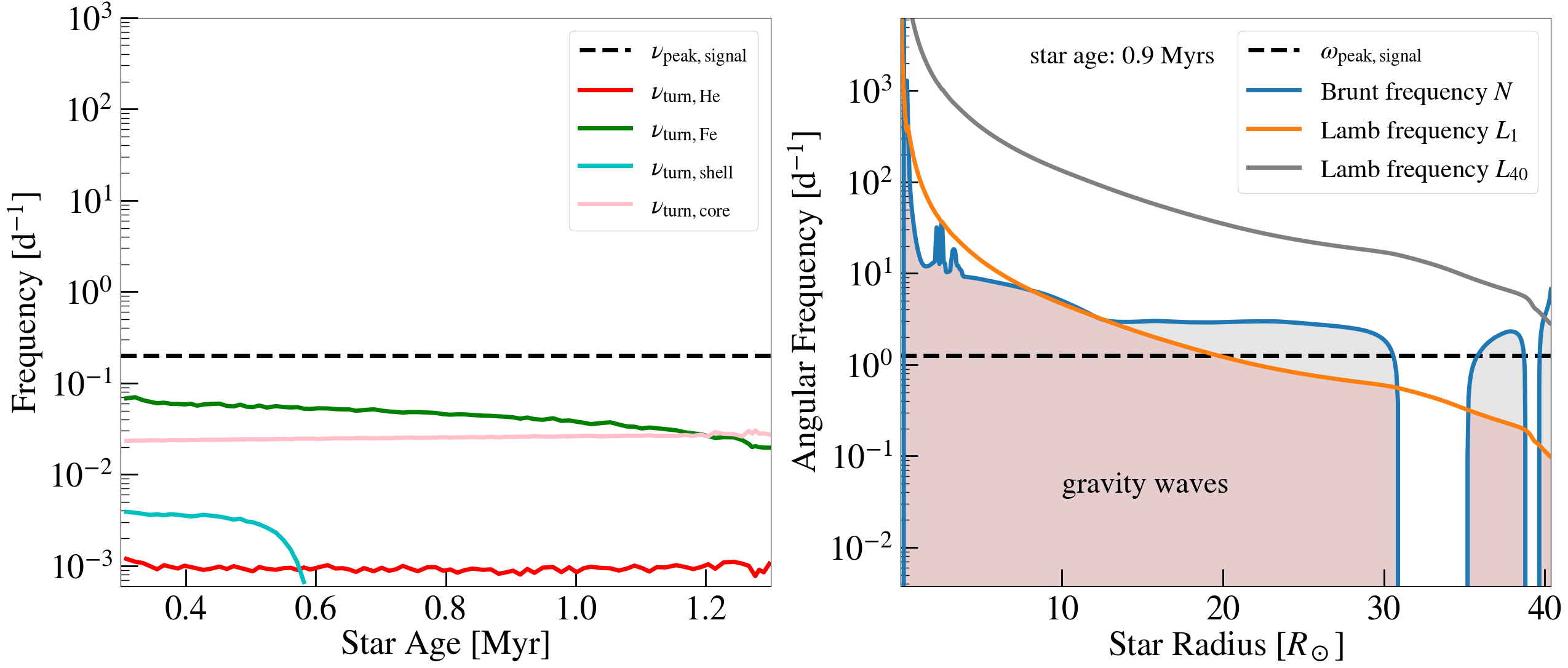
Figure 8: Left: the convective turnover frequencies for the convective zones in our BSG model. The frequencies corresponding to the iron opacity peak convective zone and core convection are the closest to the peak frequency of the signal. Right: the propagation diagram for the stellar model at $0.9$ Myr, where the colored/grey shaded regions show the frequencies where $l=1$ and $l=40$ gravity waves can propagate. The regions where Brunt frequency vanishes are the two subsurface convective zones.

If subsurface convection causes low-frequency variability in some signal, Cantiello et al. (2021) points out that the characteristic frequency of the signal should match the convective turnover frequency on top of the subsurface convection zone. In the left panel of Figure 8 we plot these frequencies of the convective zones in our BSG models (including two subsurface zones caused by opacity peaks, a convective zone above the burning shell before 0.6 Myr, and burning the convective core, see Figure 7 for reference), calculated by $\nu_{\mathrm{turn}}=(2\pi\alpha_{\mathrm{MLT}}\bar{H}_{\mathrm{P}}/\bar{v}_{\mathrm{c}})^{-1}$ (with $\alpha_{\mathrm{MLT}}=2.0$, see Section 3 in Cantiello et al. 2021 for details), along with the typical peak frequency in our signal $\nu_{\mathrm{peak}}=0.2\,\mathrm{d}$. The results seem to favor the convective zone related to iron opacity peak, whose turnover frequency on top is only lower than the signal frequency by a factor of a few, and the inconsistency may only be caused by the uncertainty of $\alpha_{\mathrm{MLT}}$ (Cantiello et al., 2021). The frequencies of other convective zones are either too low, or the zones themselves are too deep to create any surface convective motion. However, as 3D simulations found that convective zones could extend spatially to larger scales than MLT predictions (Schultz et al., 2022), we should keep in mind that the two subsurface convective zones may actually merge together, and make our MLT calculations unreliable.

In addition, we note that (sub)surface convection and granulation are mostly discussed to explain red noise signals (see, e.g., Kallinger et al. 2014), which is different from the characteristic shape of our signal, as the former usually levels off at zero frequency, where our power spectra vanishes. Physically, one would not expect incoherent convective motion to have some longest cut-off periodicity, creating a decay of power towards lower frequency. This means convective motion is not satisfactory to explain the shape of our signal in general.

5.3 Internal Gravity Waves and Pulsating g-modes

Internal oscillations have also been suggested as origins of low-frequency photometric variability for massive stars. These oscillations could be waves that propagate to the stellar surface (Cantiello et al., 2009b; Bowman et al., 2019a; Ratnasingam et al., 2020), or pulsating modes that are trapped inside the stars (Shiode et al., 2013). They can be driven by the $\kappa$-mechanism associated with iron opacity peaks, which is responsible for non-stable pulsations in $\beta$ Cephei stars and slowly pulsating B stars (see, e.g., Pamyatnykh 1999; Dupret 2001), or excited stochastically by turbulent convective motion (see, e.g., Lecoanet et al. 2021; Thompson et al. 2023). In BSGs with convective zones caused by the iron opacity peak, in pricinple both mechanisms could be related. Nevertheless, the stochasticity in our signal seems to favor convective excitation, and recent 3D simulations showed that modes excited this way can have lifetimes as short as $\sim 10$ days (Thompson et al., 2023), consistent with our findings (see Section 3.2).

It has been proposed that several types of waves may propagate in stars that create low-frequency signal, including Rossby waves that are restored by Coriolis force (Van Reeth et al., 2016; Saio et al., 2018) and gravity waves that are restored by buoyancy (Cantiello et al., 2021; Schultz et al., 2022). Among them, we point out that damped gravity waves may naturally explain the shape of our signal at the low-frequency end: with shorter wavelengths at longer periods, gravity waves are preferentially damped at lower-frequency when they propagate in stellar radiative zones, creating smaller photometric amplitudes when they reach the surface. This is exactly what we found from our signal, and has been verified by recent 3D simulations on wave propagation (see Figure 2 in Anders et al. 2023).

Goldreich & Kumar (1990) showed that if gravity waves are excited by convective motion, they should have a peak power around the convective turnover frequency on top of that convective zone. We hence showed these frequencies calculated for the different convective zones from our BSG model in the left panel of Figure 8, compared to the typical peak frequency in our signal $\nu_{\mathrm{peak}}=0.2\,\mathrm{d}$. We see that the convective turnover frequencies on top of the iron-opacity convective zone and the convective core are both within an order of magnitude lower than the observed peak frequency of the signal (an uncertainty tolerated by the choice of $\alpha_{\mathrm{MLT}}$, see Section 5.2), suggesting they might generate a spectrum of waves that can be interpreted as our signal. We note, however, Anders et al. (2023) points out that waves generated from the core cannot get to the observed amplitude when they reach the surface, though in their simulations they did not have other convective zones above the core, which may amplify or further damp the wave amplitude and it travels through them.

To see whether gravity waves excited by convection can propagate, we show the propagation diagram (i.e., the parameter space of the angular frequencies and locations inside a star where waves can propagate) in the right panel of Figure 8, for our BSG model at a typical stellar age of $0.9\,\mathrm{Myr}$. Gravity waves can only propagate in regions where their frequencies are below both the Brunt-Väisälä frequency and the Lamb frequency (Unno et al., 1989). We see that for $l=1$ waves, the cut-off frequency above the iron opacity peak is below the peak frequency we find in our signal, which means waves at our peak frequency evanescent. Nevertheless, Cantiello et al. (2009a) and Shiode et al. (2013) demonstrated that gravity waves excited by subsurface convection can have very high degrees ($l\gtrsim 30$), whose cut-off frequencies are above the peak frequency of our signal (see Figure 8 for the propagation of an example $l=40$ wave), such that they may propagate to the surface. However, these high-degree oscillations may only produce small amplitudes because of geometric cancellation effects, and it is questionable whether they are detectable.

An additional constraint from the signal is that there are no individual modes identified for any of our BSGs around the characteristic peak frequency. Bellinger et al. (2023) proposed that if BSGs are formed by mergers, the $l=1$ g-mode period spacing would be $\Delta\Pi_{1}\approx 20-30\,\mathrm{min}$. To identify individual g modes around $\nu_{\mathrm{peak}}\sim 0.2\,\mathrm{d}^{-1}$, this requires the frequency resolution to be less than $\Delta\nu=\nu_{\mathrm{peak}}^{2}\Delta\Pi\approx 10^{-3}\,\mathrm{d}^{-1}$, marginally below the resolution of the full TESS light curves of our sample. For higher-degree g modes, their geometric cancellation effects make it impossible to identify them from photometry. Therefore, the lack of identified modes from the signal still could not exclude the possibility that they are a spectrum of individual g-modes. Nevertheless, we expect further observations with increased photometric precision (such as those with the PLATO mission; Miglio et al. 2017) and observations seeking for spectroscopic time variability will help to distinguish these modes.

We note, however, that our wave analysis is based on timescale arguments on this single 1D stellar evolution model. More detailed investigation including solving oscillation modes/3D modelling of convection should be carried out to testify this explanation in the future.

6 Conclusion

In this manuscript, we analyzed TESS light curves for 20 blue supergiants (BSGs) in the LMC, and found a characteristic signal in the low-frequency ($f\lesssim 2\,\mathrm{d}^{-1}$) range for all our targets. The signals show strong stochasticity across different TESS sectors, yet their full power spectrum show a peak frequency around $0.2\,\mathrm{d}^{-1}$, below which the power tends to zero. We were able to fit the signal with a modified Lorentzian profile (Equation 1), and the fitting parameters have no strong correlations with spectroscopic parameters measured for these systems.

We compared our signals to those obtained from a limited sample of hotter OB stars, yellow supergiants, alpha Cygni variables and red supergiants. We see similarities between our signal and the low-frequency variability of hot OB stars, yellow supergiants and some alpha Cygni variables. This comparison, while limited, may suggest the origins of these signals are similar.

We discussed three possible mechanisms that may explain this signal: stellar winds launched by rotation, subsurface convective motion and internal oscillations of the star. The spectroscopic measured $v\sin i$ seems to disfavor the wind mechanism, as they would produce too low a characteristic frequency compared to the signal. We made a BSG model to test the latter two scenarios, and we found that the turnover frequency on top of the convective zone caused by iron opacity peak is consistent the peak frequency of the signal, despite the uncertainties introduced by the choice of mixing length parameter. While convective motion in this zone may be interpreted as the signal, it might be too deep to be directly observed in the photosphere, and such motions typically do not predict the shape of our power spectra. High-order, damped gravity waves excited from this convective zone seem to be a better explanation, which explains both the peak frequency and the shape of the signal, though this picture will require more thorough investigation.

We restricted our sample to 20 BSGs with reliable TESS time series and spectroscopic parameters in the LMC. While this gives a clean sample to draw away the signal, we do not know whether it is still present for higher-metallicity BSGs. In future work we will extend our analysis to more Galactic BSGs. A greater population of sample may also help us to seek for potential correlations between the signal and stellar parameters.

Our theoretical analysis is somewhat limited by the single BSG model we choose, and future works should also focus on more detailed modelling of the BSGs in our sample.

Appendix A TESS Light Curves for All Our BSGs

In Figures 9 to 28 we present the light curves and periodograms of all our BSG sample. They show a universal pattern in the low-frequency range.

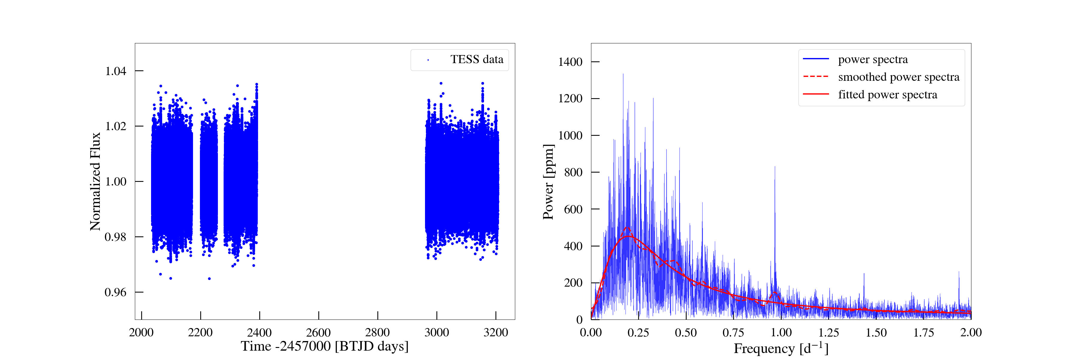
Figure 9: TESS data and power density spectra of SK -68 53 (TIC31179797). The smoothed and fitted spectrum are shown in dashed and solid red lines.

Figure 10: TESS data and power density spectra of SK -66 125 (TIC425086354). The smoothed and fitted spectrum are shown in dashed and solid red lines.

Figure 11: TESS data and power density spectra of SK -67 283 (TIC31511729). The smoothed and fitted spectrum are shown in dashed and solid red lines.

Figure 12: TESS data and power density spectra of SK -69 31 (TIC30190076). The smoothed and fitted spectrum are shown in dashed and solid red lines.

Figure 22: TESS data and power density spectra of HD 269510 (TIC373682056). The smoothed and fitted spectrum are shown in dashed and solid red lines.

Figure 23: TESS data and power density spectra of SK -66 92 (TIC373845622). The smoothed and fitted spectrum are shown in dashed and solid red lines.

Figure 24: TESS data and power density spectra of SK -67 151 (TIC391809264). The smoothed and fitted spectrum are shown in dashed and solid red lines.

References

- Aerts et al. (2010) Aerts, C., Lefever, K., Baglin, A., et al. 2010, A&A, 513, L11, doi: 10.1051/0004-6361/201014124
- Aerts et al. (2017) Aerts, C., Símon-Díaz, S., Bloemen, S., et al. 2017, A&A, 602, A32, doi: 10.1051/0004-6361/201730571
- Aerts et al. (2018) Aerts, C., Bowman, D. M., Símon-Díaz, S., et al. 2018, MNRAS, 476, 1234, doi: 10.1093/mnras/sty308
- Anders et al. (2023) Anders, E. H., Lecoanet, D., Cantiello, M., et al. 2023, Nature Astronomy, doi: 10.1038/s41550-023-02040-7
- Astropy Collaboration et al. (2013) Astropy Collaboration, Robitaille, T. P., Tollerud, E. J., et al. 2013, A&A, 558, A33, doi: 10.1051/0004-6361/201322068
- Astropy Collaboration et al. (2018) Astropy Collaboration, Price-Whelan, A. M., Sipőcz, B. M., et al. 2018, AJ, 156, 123, doi: 10.3847/1538-3881/aabc4f
- Astropy Collaboration et al. (2022) Astropy Collaboration, Price-Whelan, A. M., Lim, P. L., et al. 2022, apj, 935, 167, doi: 10.3847/1538-4357/ac7c74
- Auvergne et al. (2009) Auvergne, M., Bodin, P., Boisnard, L., et al. 2009, A&A, 506, 411, doi: 10.1051/0004-6361/200810860
- Bellinger et al. (2023) Bellinger, E., de Mink, S., van Rossem, W., & Justham, S. 2023, submitted
- Blomme et al. (2011) Blomme, R., Mahy, L., Catala, C., et al. 2011, A&A, 533, A4, doi: 10.1051/0004-6361/201116949
- Borucki et al. (2010) Borucki, W. J., Koch, D., Basri, G., et al. 2010, Science, 327, 977, doi: 10.1126/science.1185402
- Bowman et al. (2020) Bowman, D. M., Burssens, S., Simón-Díaz, S., et al. 2020, A&A, 640, A36, doi: 10.1051/0004-6361/202038224
- Bowman & Dorn-Wallenstein (2022) Bowman, D. M., & Dorn-Wallenstein, T. Z. 2022, A&A, 668, A134, doi: 10.1051/0004-6361/202243545
- Bowman et al. (2019a) Bowman, D. M., Burssens, S., Pedersen, M. G., et al. 2019a, Nature Astronomy, 3, 760, doi: 10.1038/s41550-019-0768-1
- Bowman et al. (2019b) Bowman, D. M., Aerts, C., Johnston, C., et al. 2019b, A&A, 621, A135, doi: 10.1051/0004-6361/201833662
- Braun & Langer (1995) Braun, H., & Langer, N. 1995, A&A, 297, 483
- Brott et al. (2011) Brott, I., de Mink, S. E., Cantiello, M., et al. 2011, A&A, 530, A115, doi: 10.1051/0004-6361/201016113
- de Burgos et al. (2023) de Burgos, A., Simón-Díaz, S., Urbaneja, M. A., & Negueruela, I. 2023, A&A, 674, A212, doi: 10.1051/0004-6361/202346179
- Cantiello et al. (2009a) Cantiello, M., Langer, N., Brott, I., et al. 2009a, Communications in Asteroseismology, 158, 61, doi: 10.48550/arXiv.0810.2546
- Cantiello et al. (2021) Cantiello, M., Lecoanet, D., Jermyn, A. S., & Grassitelli, L. 2021, ApJ, 915, 112, doi: 10.3847/1538-4357/ac03b0
- Cantiello et al. (2009b) Cantiello, M., Langer, N., Brott, I., et al. 2009b, A&A, 499, 279, doi: 10.1051/0004-6361/200911643
- Castro et al. (2014) Castro, N., Fossati, L., Langer, N., et al. 2014, A&A, 570, L13, doi: 10.1051/0004-6361/201425028
- Castro et al. (2018) Castro, N., Oey, M. S., Fossati, L., & Langer, N. 2018, ApJ, 868, 57, doi: 10.3847/1538-4357/aae6d0
- Chaplin & Miglio (2013) Chaplin, W. J., & Miglio, A. 2013, ARA&A, 51, 353, doi: 10.1146/annurev-astro-082812-140938
- Choi et al. (2016) Choi, J., Dotter, A., Conroy, C., et al. 2016, ApJ, 823, 102, doi: 10.3847/0004-637X/823/2/102
- Dekker et al. (2000) Dekker, H., D’Odorico, S., Kaufer, A., Delabre, B., & Kotzlowski, H. 2000, in Society of Photo-Optical Instrumentation Engineers (SPIE) Conference Series, Vol. 4008, Optical and IR Telescope Instrumentation and Detectors, ed. M. Iye & A. F. Moorwood, 534–545, doi: 10.1117/12.395512
- Dorn-Wallenstein et al. (2019) Dorn-Wallenstein, T. Z., Levesque, E. M., & Davenport, J. R. A. 2019, ApJ, 878, 155, doi: 10.3847/1538-4357/ab223f
- Dorn-Wallenstein et al. (2022) Dorn-Wallenstein, T. Z., Levesque, E. M., Davenport, J. R. A., et al. 2022, ApJ, 940, 27, doi: 10.3847/1538-4357/ac79b2
- Dorn-Wallenstein et al. (2020) Dorn-Wallenstein, T. Z., Levesque, E. M., Neugent, K. F., et al. 2020, ApJ, 902, 24, doi: 10.3847/1538-4357/abb318
- Dotter (2016) Dotter, A. 2016, ApJS, 222, 8, doi: 10.3847/0067-0049/222/1/8
- Dupret (2001) Dupret, M. A. 2001, A&A, 366, 166, doi: 10.1051/0004-6361:20000219
- Eisner et al. (2020) Eisner, N., Lintott, C., & Aigrain, S. 2020, The Journal of Open Source Software, 5, 2101, doi: 10.21105/joss.02101
- Farrell et al. (2019) Farrell, E. J., Groh, J. H., Meynet, G., et al. 2019, A&A, 621, A22, doi: 10.1051/0004-6361/201833657
- Gaia Collaboration et al. (2018) Gaia Collaboration, Brown, A. G. A., Vallenari, A., et al. 2018, A&A, 616, A1, doi: 10.1051/0004-6361/201833051
- Gaia Collaboration et al. (2023) Gaia Collaboration, Vallenari, A., Brown, A. G. A., et al. 2023, A&A, 674, A1, doi: 10.1051/0004-6361/202243940
- Goldreich & Kumar (1990) Goldreich, P., & Kumar, P. 1990, ApJ, 363, 694, doi: 10.1086/169376
- Hekker & Christensen-Dalsgaard (2017) Hekker, S., & Christensen-Dalsgaard, J. 2017, A&A Rev., 25, 1, doi: 10.1007/s00159-017-0101-x
- Hofmeister et al. (1964) Hofmeister, E., Kippenhahn, R., & Weigert, A. 1964, ZAp, 59, 242
- Hoyle (1960) Hoyle, F. 1960, MNRAS, 120, 22, doi: 10.1093/mnras/120.1.22
- Jenkins et al. (2016) Jenkins, J. M., Twicken, J. D., McCauliff, S., et al. 2016, in Society of Photo-Optical Instrumentation Engineers (SPIE) Conference Series, Vol. 9913, Software and Cyberinfrastructure for Astronomy IV, ed. G. Chiozzi & J. C. Guzman, 99133E, doi: 10.1117/12.2233418
- Jermyn et al. (2023) Jermyn, A. S., Bauer, E. B., Schwab, J., et al. 2023, ApJS, 265, 15, doi: 10.3847/1538-4365/acae8d
- Justham et al. (2014) Justham, S., Podsiadlowski, P., & Vink, J. S. 2014, ApJ, 796, 121, doi: 10.1088/0004-637X/796/2/121
- Kaiser et al. (2020) Kaiser, E. A., Hirschi, R., Arnett, W. D., et al. 2020, MNRAS, 496, 1967, doi: 10.1093/mnras/staa1595
- Kallinger et al. (2014) Kallinger, T., De Ridder, J., Hekker, S., et al. 2014, A&A, 570, A41, doi: 10.1051/0004-6361/201424313
- Kaufer et al. (1999) Kaufer, A., Stahl, O., Tubbesing, S., et al. 1999, The Messenger, 95, 8
- Klencki et al. (2020) Klencki, J., Nelemans, G., Istrate, A. G., & Pols, O. 2020, A&A, 638, A55, doi: 10.1051/0004-6361/202037694
- Kobulnicky & Fryer (2007) Kobulnicky, H. A., & Fryer, C. L. 2007, ApJ, 670, 747, doi: 10.1086/522073
- Krtička & Feldmeier (2018) Krtička, J., & Feldmeier, A. 2018, A&A, 617, A121, doi: 10.1051/0004-6361/201731614
- Krtička & Feldmeier (2021) —. 2021, A&A, 648, A79, doi: 10.1051/0004-6361/202040148
- Langer & Kudritzki (2014) Langer, N., & Kudritzki, R. P. 2014, A&A, 564, A52, doi: 10.1051/0004-6361/201423374
- Laplace et al. (2020) Laplace, E., Götberg, Y., de Mink, S. E., Justham, S., & Farmer, R. 2020, A&A, 637, A6, doi: 10.1051/0004-6361/201937300
- Lecoanet et al. (2021) Lecoanet, D., Cantiello, M., Anders, E. H., et al. 2021, MNRAS, 508, 132, doi: 10.1093/mnras/stab2524
- van Leeuwen et al. (1998) van Leeuwen, F., van Genderen, A. M., & Zegelaar, I. 1998, A&AS, 128, 117, doi: 10.1051/aas:1998129
- Lightkurve Collaboration et al. (2018) Lightkurve Collaboration, Cardoso, J. V. d. M., Hedges, C., et al. 2018, Lightkurve: Kepler and TESS time series analysis in Python, Astrophysics Source Code Library. http://ascl.net/1812.013
- Martinet et al. (2021) Martinet, S., Meynet, G., Ekström, S., et al. 2021, A&A, 648, A126, doi: 10.1051/0004-6361/202039426
- Michel et al. (2008) Michel, E., Baglin, A., Auvergne, M., et al. 2008, Science, 322, 558, doi: 10.1126/science.1163004
- Miglio et al. (2017) Miglio, A., Chiappini, C., Mosser, B., et al. 2017, Astronomische Nachrichten, 338, 644, doi: 10.1002/asna.201713385
- de Mink et al. (2013) de Mink, S. E., Langer, N., Izzard, R. G., Sana, H., & de Koter, A. 2013, ApJ, 764, 166
- de Mink et al. (2014) de Mink, S. E., Sana, H., Langer, N., Izzard, R. G., & Schneider, F. R. N. 2014, ApJ, 782, 7, doi: 10.1088/0004-637X/782/1/7
- Neugent et al. (2020) Neugent, K. F., Levesque, E. M., Massey, P., Morrell, N. I., & Drout, M. R. 2020, ApJ, 900, 118, doi: 10.3847/1538-4357/ababaa
- Owocki & Rybicki (1984) Owocki, S. P., & Rybicki, G. B. 1984, ApJ, 284, 337, doi: 10.1086/162412
- Pamyatnykh (1999) Pamyatnykh, A. A. 1999, Acta Astron., 49, 119
- Paxton et al. (2011) Paxton, B., Bildsten, L., Dotter, A., et al. 2011, ApJS, 192, 3, doi: 10.1088/0067-0049/192/1/3
- Paxton et al. (2013) Paxton, B., Cantiello, M., Arras, P., et al. 2013, ApJS, 208, 4, doi: 10.1088/0067-0049/208/1/4
- Paxton et al. (2015) Paxton, B., Marchant, P., Schwab, J., et al. 2015, ApJS, 220, 15, doi: 10.1088/0067-0049/220/1/15
- Paxton et al. (2018) Paxton, B., Schwab, J., Bauer, E. B., et al. 2018, ApJS, 234, 34, doi: 10.3847/1538-4365/aaa5a8
- Paxton et al. (2019) Paxton, B., Smolec, R., Schwab, J., et al. 2019, ApJS, 243, 10, doi: 10.3847/1538-4365/ab2241
- Pedersen & Bell (2023) Pedersen, M. G., & Bell, K. J. 2023, AJ, 165, 239, doi: 10.3847/1538-3881/accc31
- Pedersen et al. (2019) Pedersen, M. G., Chowdhury, S., Johnston, C., et al. 2019, ApJ, 872, L9, doi: 10.3847/2041-8213/ab01e1
- Podsiadlowski et al. (1992) Podsiadlowski, P., Joss, P. C., & Hsu, J. J. L. 1992, ApJ, 391, 246, doi: 10.1086/171341
- Puls et al. (2006) Puls, J., Markova, N., Scuderi, S., et al. 2006, A&A, 454, 625, doi: 10.1051/0004-6361:20065073
- Puls et al. (2008) Puls, J., Vink, J. S., & Najarro, F. 2008, A&A Rev., 16, 209, doi: 10.1007/s00159-008-0015-8
- Puls et al. (1996) Puls, J., Kudritzki, R. P., Herrero, A., et al. 1996, A&A, 305, 171
- Ramiaramanantsoa et al. (2018) Ramiaramanantsoa, T., Moffat, A. F. J., Harmon, R., et al. 2018, MNRAS, 473, 5532, doi: 10.1093/mnras/stx2671
- Ratnasingam et al. (2020) Ratnasingam, R. P., Edelmann, P. V. F., & Rogers, T. M. 2020, MNRAS, 497, 4231, doi: 10.1093/mnras/staa2296
- Ricker et al. (2015) Ricker, G. R., Winn, J. N., Vanderspek, R., et al. 2015, Journal of Astronomical Telescopes, Instruments, and Systems, 1, 014003, doi: 10.1117/1.JATIS.1.1.014003
- Saio et al. (2018) Saio, H., Kurtz, D. W., Murphy, S. J., Antoci, V. L., & Lee, U. 2018, MNRAS, 474, 2774, doi: 10.1093/mnras/stx2962
- Sana et al. (2012) Sana, H., de Mink, S. E., de Koter, A., et al. 2012, Science, 337, 444, doi: 10.1126/science.1223344
- Schootemeijer et al. (2019) Schootemeijer, A., Langer, N., Grin, N. J., & Wang, C. 2019, A&A, 625, A132, doi: 10.1051/0004-6361/201935046
- Schultz et al. (2022) Schultz, W. C., Bildsten, L., & Jiang, Y.-F. 2022, ApJ, 924, L11, doi: 10.3847/2041-8213/ac441f
- Schultz et al. (2023a) —. 2023a, ApJ, 951, L42, doi: 10.3847/2041-8213/acdf50
- Schultz et al. (2023b) Schultz, W. C., Tsang, B. T. H., Bildsten, L., & Jiang, Y.-F. 2023b, ApJ, 945, 58, doi: 10.3847/1538-4357/acb701
- Schwarzschild (1975) Schwarzschild, M. 1975, ApJ, 195, 137, doi: 10.1086/153313
- Serebriakova et al. (2023) Serebriakova, N., Tkachenko, A., Gebruers, S., et al. 2023, A&A, 676, A85, doi: 10.1051/0004-6361/202346108
- Shiode et al. (2013) Shiode, J. H., Quataert, E., Cantiello, M., & Bildsten, L. 2013, MNRAS, 430, 1736, doi: 10.1093/mnras/sts719
- Simón-Díaz et al. (2017) Simón-Díaz, S., Godart, M., Castro, N., et al. 2017, A&A, 597, A22, doi: 10.1051/0004-6361/201628541
- Simón-Díaz & Herrero (2014) Simón-Díaz, S., & Herrero, A. 2014, A&A, 562, A135, doi: 10.1051/0004-6361/201322758
- Szewczuk et al. (2021) Szewczuk, W., Walczak, P., & Daszyńska-Daszkiewicz, J. 2021, MNRAS, 503, 5894, doi: 10.1093/mnras/stab683
- Thompson et al. (2023) Thompson, W., Herwig, F., Woodward, P. R., et al. 2023, arXiv e-prints, arXiv:2303.06125, doi: 10.48550/arXiv.2303.06125
- Unno et al. (1989) Unno, W., Osaki, Y., Ando, H., Saio, H., & Shibahashi, H. 1989, Nonradial oscillations of stars (University of Tokyo Press)
- Van Reeth et al. (2016) Van Reeth, T., Tkachenko, A., & Aerts, C. 2016, A&A, 593, A120, doi: 10.1051/0004-6361/201628616
- Vanbeveren et al. (2013) Vanbeveren, D., Mennekens, N., Van Rensbergen, W., & De Loore, C. 2013, A&A, 552, A105, doi: 10.1051/0004-6361/201321072
- Virtanen et al. (2020) Virtanen, P., Gommers, R., Oliphant, T. E., et al. 2020, Nature Methods, 17, 261, doi: 10.1038/s41592-019-0686-2
- Walborn et al. (1987) Walborn, N. R., Lasker, B. M., Laidler, V. G., & Chu, Y.-H. 1987, ApJ, 321, L41, doi: 10.1086/185002
- Weiss (1989) Weiss, A. 1989, ApJ, 339, 365, doi: 10.1086/167302
- Wenger et al. (2000) Wenger, M., Ochsenbein, F., Egret, D., et al. 2000, A&AS, 143, 9, doi: 10.1051/aas:2000332