Exploiting Image-Related Inductive Biases in Single-Branch Visual Tracking

Abstract

Despite achieving state-of-the-art performance in visual tracking, recent single-branch trackers tend to overlook the weak prior assumptions associated with the Vision Transformer (ViT) encoder and inference pipeline. Moreover, the effectiveness of discriminative trackers remains constrained due to the adoption of the dual-branch pipeline. To tackle the inferior effectiveness of the vanilla ViT, we propose an Adaptive ViT Model Prediction tracker (AViTMP) to bridge the gap between single-branch network and discriminative models. Specifically, in the proposed encoder AViT-Enc, we introduce an adaptor module and joint target state embedding to enrich the dense embedding paradigm based on ViT. Then, we combine AViT-Enc with a dense-fusion decoder and a discriminative target model to predict accurate location. Further, to mitigate the limitations of conventional inference practice, we present a novel inference pipeline called CycleTrack, which bolsters the tracking robustness in the presence of distractors via bidirectional cycle tracking verification. Lastly, we propose a dual-frame update inference strategy that adeptively handles significant challenges in long-term scenarios. In the experiments, we evaluate AViTMP on ten tracking benchmarks for a comprehensive assessment, including LaSOT, LaSOTExtSub, AVisT, etc. The experimental results unequivocally establish that AViTMP attains state-of-the-art performance, especially on long-time tracking and robustness. The source code will be released upon acceptance.

I Introduction

Generic object visual tracking is a significant challenge in computer vision, as it involves the estimation of the target’s position in each frame based on the target bounding box of the initial frame. This problem holds great importance in various practical applications, including autonomous driving [1, 2], intelligent surveillance [3, 4, 5, 6], and advanced traffic systems [7, 8, 9]. Among the prevailing tracking techniques, the discriminative trackers, Siamese trackers, and single-branch trackers stand out as prominent pipelines. discriminative approaches [10, 11, 12, 13, 14] learn the target model to localize the target position by minimizing a discriminative objective function. Siamese trackers [15, 16, 17, 18] learn the similarity matrix to classify and locate the foreground and background based on two branches of feature matching. Recently, there has been a surge in the popularity of single-branch trackers [19, 20, 21, 22, 23] as widely adopted in various applications. These frameworks apply a straightforward single-branch Vision Transformer (ViT) to perform internal cross-matching tasks and achieve state-of-the-art performance. Typical single-branch trackers [19, 20, 23] follow a similar pipeline where flattened frames are concatenated together. They then directly employ vanilla ViT to facilitate information interaction by means of self-attention blocks across multiple frames.

Compared with the hierarchical variants [24, 25] and vision-specific transformers [26], the vanilla ViT lacks image-related prior knowledge, which results in slower convergence and suboptimal performance [27], especially on dense prediction tasks. Therefore, the vanilla ViT, used in most single-branch trackers, suffers from inferior performance on visual tracking due to weak prior assumptions and lack of vision-specific inductive biases and may not achieve optimal performance.

To address this challenge, we introduce an Adaptive ViT that leverages spatial priors and vision-specific inductive biases. More specifically, in the encoding phase, we prioritize the utilization of target spatial-prior information and position priors using the Adaptive ViT. This encoded feature becomes a reference for prediction in subsequent phases. subsequent decoder module generates target model weights. During the model prediction process, our framework employs the discriminative target model for accurate target prediction. As a result, AViTMP establishes an optimal paradigm for feature aggregation and target prediction, obtaining excellent performance in object tracking. Furthermore, different from recent single-branch trackers which discard important background information by cropping template frames, AViTMP directly uses all original whole frames without target-centered cropping as the training frame to discriminate the target frame feature from the background. As such, AViTMP bridges the gap between recent dual-branch discriminate models and the single-branch paradigm, achieving state-of-the-art tracking performance in most attributes.

Another drawback of current single-branch trackers is that the simple network design and inference pipeline fails to account for a pivotal tracking characteristic: methods should consider the temporal consistency of the target position among distinct frames for sequence prediction. The current ViT-based networks are all based on template updates to achieve a bit better long-time robust tracking performance but hardly exploit the location along the temporal dimension, potentially leading to mis-track distractors in current approaches [21, 20, 23]. To address this challenge, regarding the exploitation of the temporal nature of tracking, we propose an innovative inference approach named CycleTrack, aimed at achieving robust tracking performance in the presence of distractors. During the inference phase, we incorporate a candidate discrimination module that assesses the reliability of the predicted target candidate. This mechanism examines the temporal cycle consistency between the present frame and the stored previous frame and then opts for a candidate that demonstrates better alignment with this consistency. The effect of applying the CycleTrack in the inference stage is illustrated in Figure 4, where we consider choosing the higher temporal consistency prediction result as the final location. Additionally, we propose a dual-frames update inference strategy to overcome the degradation of frames particularly in long-term sequences. That mainly occurs in those scenarios involving significant deformations, scale variations, or domain shifts.

To summarize, our contributions are listed as follows:

• We propose a single-branch transformer model prediction tracker AViTMP, which is built by an adaptive ViT encoder with a dense-fused decoder and target predictor. AViTMP optimizes the feature encoding and decoding phases to optimally exploit image-related inductive biases for single-branch tracking.

• In addition, we propose a novel CycleTrack inference mechanism to enhance the temporal consistency of target location in long-term tracking with few testing costs and without training costs. A dual-frame update strategy is introduced to consider the degradation of the initial frame, guaranteeing robust long-term tracking.

• We perform comprehensive experiments to assess the contribution of each element and AViTMP achieves state-of-the-art performance and real-time speed on multiple benchmarks.

II Related Works

In this section, we will give a brief review of visual object-tracking networks and online inference strategies. More related works can be found in the following survey papers [28, 29].

Visual Object Tracking.  Generally, visual tracking can be divided into three streams.  i.) The Siamese tracking paradigm [15, 30, 31, 17] conceptualizes tracking as a task involving similarity matching between frames and employs a weight-shared dual-branch backbone. Building upon the contextual interaction and modeling abilities of transformers [32, 33], Siamese trackers have evolved to incorporate Transformers [16, 34, 35, 18] recently.  ii.) Discriminative approaches [11, 12, 36] distinguish the target by minimizing a discriminative objective function. KeepTrack [37] introduces a learned association network to discern distractors, thereby enhancing tracking robustness. Bridging the gap between Transformer and discriminative paradigms, ToMP [38] integrates a Transformer encoder-decoder module into a concise discriminative target localization model. Similar to the Siamese framework, discriminative approaches also contain two parallel branches for segregated feature extraction of training and testing frames, constituting a dual-stream paradigm.  iii.) Single-branch trackers [19, 39, 22] consolidate feature extraction and interaction ability within a single branch backbone. SimTrack [19] simplifies the dual-stream feature extraction networks into a unified process and pioneers the introduction of ViT [40] into visual tracking. MixFormer [21] utilizes a variant of ViT (named CVT [41]) as its one-branch backbone while splitting the template and search patches for patch embedding at each stage of the backbone. OSTrack [23] joint feature learning and relation modelling in the one-stream ViT network and integrates a candidate early elimination module after each ViT layer to expedite the inference speed. SeqTrack [20] employs a vanilla ViT encoder and causal transformer decoder to locate the target autoregressively. GRM [39] also employs a vanilla ViT but flexibly switches the framework to two-stream or single-branch based on token division.
    However, current prevailing trackers commonly employ the conventional transformer (i.e., VIT [40], Swin [24], etc) and their variants to extract features and enhance performance, yet without any trackers tailored adaptations of backbone to suit the unique demands of the tracking task. Based on the premise that the most recently popular and efficient Transformer backbone in visual tracking is ViT [20, 23, 39, 21, 19], as a purpose of this paper, we aim to extend the naive ViT architecture specifically tailored for the visual tracking task. Generally, current trackers use the base version transformer (i.e., Swin-Base, ViT-Base) for a fair comparison, while some trackers present performance-oriented variants by using large version backbones (i.e., Swin-Large, ViT-Large) and large resolution. In this work, different from performance-oriented trackers, we compared the performance with the same base version of the backbone and similar resolutions (256 or 288) for a fair comparison, making it convenient to verify the effectiveness of each design under limited platforms (GPUs).

Online Inference.  Discriminative appearance models [10, 12, 14, 42] typically incorporate background information during online learning of the target classifier to enhance appearance discriminative capabilities and suppress distractors. Nonetheless, appearance models still frequently encounter challenges in effectively distinguishing between distractors and target candidates. To address this concern, KYS [11] extend an RNN on the appearance model to propagate information across frames. KeepTrack [37] propose an association network with a self-supervised training strategy. However, these solutions introduce extra networks and training costs. Instead, our AViTMP buffers the previous historic frame information and relies on the temporal cycle consistency of the target to discern distractors during inference. On the other hand, the training-frames update [43, 34, 44], also known as template update, is a widely adopted strategy that fortifies robustness with few computational expenses. It aims to mitigate the limitations of assuming fixed reference templates. For example, Updatenet [44] proposes a network to estimate the optimal template for the next frame. LTMU [43] introduces an offline-trained meta-updater to discriminate when to update the template. STARK [18] updates the second template by replacing it when the output fulfils the specified confidence threshold and frame interval criteria. ToMP [38] updates the second training frame with a dynamic weight decline. AiATrack [34] introduces IOUNet [45] to get the IOU score and determine whether to update the current frame as a short-term template. Mixformer [21] appends a trainable network to predict the reliability score as the update condition of the second template. Nevertheless, the previous methods consistently update the second template while maintaining the first template as a fixed reference. In contrast, AViTMP offers a training-free update strategy that pioneers the update of the first reference frame for robust long-term tracking.

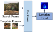
((a))

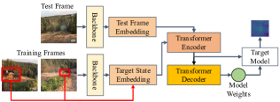
((b))

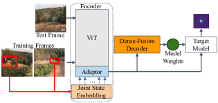
((c))

Figure 1: Comparison among trackers that employ (a) single-branch paradigm, (b) discriminative transformer model, and (c) our proposed single-branch discriminative predictor. Our model harnesses the strengths of the first two paradigms by incorporating the proposed encoder-decoder design [$\color[rgb]{.75,.75,.75}\blacksquare$$\color[rgb]{.53,.808,.98}\blacksquare$$\color[rgb]{.87,.72,.53}\blacksquare$$\color[rgb]{1,.55,0}\blacksquare$]. By this way, AViTMP integrates the powerful feature extraction capability from single-branch trackers and target prediction ability from discriminate methods into one pipeline.

III Method

In this section, we introduce an Adaptive ViT Model Prediction method, denoted as AViTMP. First, we revisit the limitations of the discriminate-based and single-branch trackers in Sec. III-A. Subsequently, we provide an overview of our proposed approach AViTMP in Sec. III-B which optimally exploits image-related inductive biases for single-branch visual tracking. Further details of the specific design are presented in Sec. III-C and Sec. III-D. Finally, we detail the online inference pipeline in Sec. III-E which exploits the temporal consistency of AViTMP without training costs.

III-A Background

Two widely recognized paradigms in visual tracking are discriminative model prediction tracking and single-branch transformer tracking. Single-branch trackers [19, 21, 22, 23] commonly integrate template and search frames into one sequence and adopt a robust and efficient backbone for feature extraction. They then proceed with classification and regression heads to predict the location of the target (Figure 1a) However, these methods apply a straightforward single-branch backbone without accounting for spatial priors and vision-specific inductive biases required for tracking, leading to suboptimal performance. On the other hand, discriminative approaches [10, 46, 12, 47] learn a target model to localize the target object in the test frame. A prominent example is ToMP (Figure 1b). Nevertheless, ToMP encodes the training and test frames independently, which hampers information integration during feature encoding. Furthermore, the divided state encoding procedure between training and test frames inhibits information interaction during the model’s initial stages. In ToMP, another drawback arises from the redundancy feature encoding process for generating discriminative features, including a CNN backbone and a Transformer Encoder, while both two involved modules are for feature encoding.

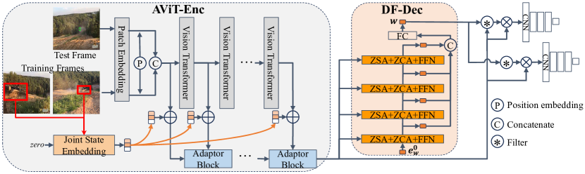
Figure 2: The overview of the architecture, including encoder (AViT-Enc), decoder (DF-Dec) and final target prediction. In AViT-Enc, training and test frames are contacted together and jointly encoded with the target prior information embedding. In DF-Dec, the encoded and adapted features are decoded and then densely integrated layer-wise to generate the model weights. Finally, the target model employs the adapted feature and model weights to predict the target location.

III-B Overview of AViTMP

To address the limitations inherent in both discriminate prediction and single-branch approaches, we present an innovative feature encoding model that replaces the existing encoding process (as depicted in Figure 1c). Instead of segregating the extraction and encoding of features into distinct stages and branches, our methodology facilitates the direct joint encoding of discriminative features from both test and training frames through a single-branch framework. By doing so, our encoding model becomes adept at incorporating the target state and specific priors right from the outset. This enables subsequent components like the decoder and target model to concentrate more on the target’s distinctive features. Additionally, in contrast to extracting a fixed feature space for test frames, this collaborative encoding process can dynamically construct an adaptive feature space connected to the training frames for every test frame.

The pipeline of our tracker is depicted in Figure 1c. Similar to discriminative trackers, the input consists of both test and training frames. Initially, we perform a joint encoding of these frames using the proposed Adaptive VIT encoder [$\color[rgb]{.75,.75,.75}\blacksquare$$\color[rgb]{.53,.808,.98}\blacksquare$$\color[rgb]{.87,.72,.53}\blacksquare$]. The joint state embedding [$\color[rgb]{.87,.72,.53}\blacksquare$] integrates target position priors into the extracted features. Subsequently, these encoded features are directed to the dense-fusion decoder [$\color[rgb]{1,.55,0}\blacksquare$] for predicting both the model weights and the target model. Ultimately, the target model discriminates the target by considering the model weights and the encoded features.

III-C Adaptive ViT Encoder

Other than standard single-branch tracking methods [19, 20, 23], our Adaptive ViT Encoder (AViT-Enc) aims to explicitly incorporate image-related inductive biases, especially by means of the proposed Adaptor module. An overview of AViT-Enc design is shown in Figure 2.

With the input test frame $x_{test}\in\mathbb{R}^{H\times W\times 3}$ and training frames $x_{i}\in\mathbb{R}^{H\times W\times 3}$, the joint encoding function is:

$$\mathcal{F}_{avit}=\mathbf{AViT}\textit{-}\mathbf{Enc}([x_{1},...,x_{m},x_{test}])\quad$$ (1)

AViT-Enc consists of four modules: Patch Embedding ($\mathbf{PE}$), Vision Transformer Blocks ($\mathbf{ViT}$), Joint State Embedding ($\mathbf{JSE}$) and Adaptor blocks ($\mathbf{Adaptor}$). The input frames are firstly flattened and projected to C-dimensional tokens by a patch embedding block. Then, they are concatenated together into a patch sequence and then add position embedding to get $\mathcal{F}^{0}_{vit}\in\mathbb{R}^{h\times w\times C}$. Here, $h=\lceil H/p\rceil$ and $w=\lceil W/p\rceil$ are denoted as the patch size of each patch. Therefore, each frame is divided into $p\times p$ non-overlapping patches. For position embedding, the same learnable position embedding [33] $\mathbf{Pos}\in\mathcal{R}^{p*p}$ is added for each test and training frame, formulated as:

$$\begin{split}\mathcal{F}^{0}_{vit}=[\mathbf{PE}(x_{test}),\mathbf{PE}(x_{1}),...,\mathbf{PE}(x_{m})]+\mathbf{Pos},\end{split}$$ (2)

Subsequent AViT blocks maintain a consistent spatial scale between the input and output. There are $L$ encoder layers in total. To adapt the vanilla ViT for tracking tasks, we embed an adaptor module inside, as shown in Figure 2.

Concretely, our approach involves a step-wise process. Initially, the first layer of AViT is directly embedded from $\mathcal{F}^{0}_{vit}$ while the following $j$-th AViT feature $\mathcal{F}^{j}_{avit}$ are obtained from adaptor block. In the context of the $j$-th layer feature of ViT denoted as $\mathcal{F}^{j}_{vit}$, the next layer feature $\mathcal{F}^{j+1}_{vit}$ is extracted by $\mathbf{ViT}_{j+1}$. Subsequently, the next AViT layer feature $\mathcal{F}^{j+1}_{avit}$ is built by the Adaptor. This process can be formulated as follows:

$$\begin{split}&\mathcal{F}^{0}_{avit}=\mathbf{JSE}(\mathcal{F}^{0}_{vit}),\\ &\mathcal{F}^{j+1}_{vit}=\mathrm{\mathbf{ViT}_{j+1}}(\mathcal{F}^{j}_{vit}),\quad\mathcal{\hat{F}}^{j+1}_{vit}=\mathbf{JSE}(\mathcal{F}^{j+1}_{vit}),\\ &\mathcal{F}^{j+1}_{avit}=\mathrm{\mathbf{Adaptor}_{j}}(\mathcal{F}^{j}_{avit},\mathcal{\hat{F}}^{j+1}_{vit})\end{split}$$ (3)

where $j\in[0,...,L-1]$. With this $L$ feature interactions, we obtain the final adaptive feature $\mathcal{F}^{L}_{avit}$. The joint state embedding is formulated to enable the integration of target location information from both the test and training frames into the encoder feature.

Joint State Embedding.  To leverage the target prior, we introduce a joint state embedding module designed to incorporate foreground center knowledge and bounding box edge information into the extracted ViT features. Particularly, for training frames, we use the learnable embedding $e_{\mathrm{fg}}\in\mathbb{R}^{1\times C}$ to represent their foreground, then the Gaussian center label $y_{i}\in\mathbb{R}^{h\times w\times 1}$ to introduce the target center inductive bias. Inspired by ToMP [38], we also introduce the target bounding box prior $d_{i}$ with a multi-layer perceptron $\phi$ to highlight the bounding box edge and to strengthen the location ability, formulated as:

$$\begin{split}&\psi_{i}=y_{i}\cdot e_{\mathrm{fg}},\quad\phi_{i}=MLP(d_{i}),\\ &\psi_{test}=\textit{zero}\cdot e_{\mathrm{fg}},\quad\phi_{test}=MLP(\textit{zero}),\\ &\mathcal{\hat{F}}^{j+1}_{vit}=\mathcal{F}^{j+1}_{vit}+[\psi_{0},...,\psi_{m},\psi_{test}]+[\phi_{0},...,\phi_{m},\phi_{test}],\end{split}$$ (4)

For each ViT layer output, our joint location embedding is weight-shared to get a unified position embedding of different feature spaces. Note that the test frame prior information is not available during inference. Therefore, in the joint location embedding process, we set the test frame location embedding as zero to keep the consistency in the training and inference phase. Existing single-branch methods ignore relevant background information by only considering the target cropped region as a template. Instead, we consider the whole source square frame as the training frame and highlight the target location via the feature embedding of the target state spatial prior.

Adaptor.  Each adaptor block is simply built by zero-center cross-attention (ZCA, inspired by [48] but simpler) and feed-forward network (FFN) with a residual connection. This process calculates the cross-attention of different feature spaces between test and training frames, further integrating the target state prior and inductive biases for tracking. Note that, different from standard attention [32, 33] which needs Sine positional encoding added before the attention, in our framework, we omit the position encoding of the adaptor block in all attention calculation processes. That means we only append different position embedding to each patch at the very beginning of AViT to avoid repeated and redundant position embedding operations of different attention layers and modules. $\textbf{Adaptor}_{j}$ block is formulated as:

$$\mathcal{\hat{F}}^{j+1}_{avit}=\mathcal{F}^{j}_{avit}+\mathbf{ZCA}\left(\mathcal{F}^{j}_{avit},\mathcal{\hat{F}}^{j+1}_{vit},\mathcal{\hat{F}}^{j+1}_{vit}\right)$$ (5)

$$\mathcal{F}^{j+1}_{avit}=\mathcal{\hat{F}}^{j+1}_{avit}+\mathbf{FFN}(\mathcal{\hat{F}}^{j+1}_{avit})$$

where ZCA block is formulated as:

$$\mathbf{ZCA}(\mathbf{Q},\mathbf{K},\mathbf{V})=softmax(\frac{\mathbf{(Q-\mu_{q})(K-\mu_{k})}^{T}}{\sqrt{d_{k}}})\mathbf{V}$$ (6)

where $\mu_{q}=\frac{1}{N}\sum_{j=1}^{N}{q_{j}}$, $\mu_{k}=\frac{1}{N}\sum_{j=1}^{N}{k_{j}}$, $N$ indicates the number of attention block heads. In contrast to the conventional attention mechanism, this modified approach constrains the tensor values within the range of (0, 1). It is inspired by the claim that attention mechanism inherently amounts to a low-pass filter and the stack of multi-head attention layers in Transformer may suppress the Alternating Current (AC) component of features severely and only left the over-smoothing Direct Current (DC) component [49, 50, 4]. Therefore, we directly remove the DC component by minus the mean value of Q and K. This can be conceptualized as a process of eliminating the DC information while retaining the AC components of the input features. Similarly, for Zero-Centered Self-Attention (ZSA), we set $\textbf{Q}==\textbf{K}$ in Eq. 6.

Finally, we obtained the AViT-Enc feature $\mathcal{F}^{L}_{avit}$ from the last adaptor layer. The adaptor has been partially motivated by Chen et al. [27] which incorporate image-related inductive biases into the transformer design. Ours, however, has a significantly different implementation. They built the adaptive ViT introducing three complex components: named spatial prior module, spatial feature injector, and multi-scale feature extractor. In contrast, our adaptor block is only built by a cross-attention and FFN block, which is an extremely lightweight component to guarantee real-time tracking.

III-D Model Predictor

Dense-Fusion Decoder.  $\mathcal{F}^{L}_{avit}$ is used as the following input of the dense-fusion decoder DF-Dec and the target model. We set another learnable embedding $e^{0}_{\mathrm{w}}\in\mathbb{R}^{1\times C}$ as the input query of our proposed DF-Dec to predict the target model weight. As shown in Figure 2, the decoder consists of N Transformer Decoder layers and a Fully-Connected (FC) layer. For each decoder layer, we adopt a zero-centered self-attention (ZSA), a zero-centered cross-attention (ZCA) and an FFN with a residual connection. The position encoding of each attention block is also removed for simplicity. The whole decoder pipeline can be written as:

$$e^{i}_{\mathrm{w}}=\mathbf{Dec}_{i}(e^{i-1}_{\mathrm{w}},\mathcal{F}^{L}_{avit}),$$ (7)

$$w=\mathbf{LN}(\mathbf{FC}[e^{0}_{\mathrm{w}},...,e^{N}_{\mathrm{w}}])$$

where $i\in[1,...,N]$, LN denotes layer normalization, and $\textbf{Dec}_{i}$ represents the $i$-th decoder layer. FC layer is used for fusing the weight embeddings of each layer to project the target model weights.

Target Model.  Following discriminative target model methods [10], we generate the target scores by the model weights and encoded features, formulated as:

$$h(w,\mathcal{F}^{L}_{avit})=w\ast\mathcal{F}^{L}_{avit}.$$ (8)

$w\in\mathbb{R}^{1\times C}$ are the weights of the convolution filter. The target model will be used in the following location heads.

Target Location.  For the two prediction heads, we use the same architecture (but without sharing weights). For the regression head, we follow ToMP [38] while with some modifications. We first adopt an FC layer to obtain the weights of regression $w_{reg}$ based on the target model weights $w$. Then, we use a filter to compute the attention weights and use the obtained attention weights multiplied point-wise with features. Lastly, the weighted features are fed into a CNN network to regress the bounding box edge $\hat{d}$ results.

$$w_{reg}=\mathbf{FC}_{1}(w),$$ (9)

$$w^{reg}_{attn}=h(w_{reg},\mathcal{F}^{L}_{avit}),$$

$$\hat{d}=\mathbf{CNN}_{1}(w^{reg}_{attn}*\mathcal{F}^{L}_{avit})$$

where the $\mathbf{CNN}_{1}$ consists of five convolutional layers. The dimension is reduced from $C$ to $\frac{C}{4}$ in the first layer and further reduced from $\frac{C}{4}$ to 4 in the last layer.

In the classification process, instead of previously used discriminative classifiers [10, 12, 38] which directly use the target model $h(w,\mathcal{F}^{L}_{avit})$ as a classification map, we keep the same procedure with our regression head except that the output dimension set as 1.

$$w_{cls}=\mathbf{FC}_{2}(w),$$ (10)

$$w^{cls}_{attn}=h(w_{cls},\mathcal{F}^{L}_{avit}),$$

$$\hat{y}=\mathbf{CNN}_{2}(w^{cls}_{attn}*\mathcal{F}^{L}_{avit})$$

where $\hat{y}$ represents the predicted foreground heat map. This design tailors the model to focus on foreground discrimination, which balances the predictions from the two heads.

Loss Functions.  For the classification head, we adopt the LBHinge [10] loss following DiMP [10]. While in the regression head, we only adopt GIOU [51] loss to converge the four edges of the predicted box. Note that we do not use the popular $L1$ loss in single-branch trackers since the full usage of the bounding box prior information can help the network converge in the joint encoding procedure. The final loss is:

$$L_{final}=\lambda L_{cls}(\hat{y},y)+L_{giou}(\hat{d},d),$$ (11)

here $\lambda=200$ is the weight to increase the classification loss magnitude for training. $y,d$ denote the Gaussian center label and ground truth prior respectively.

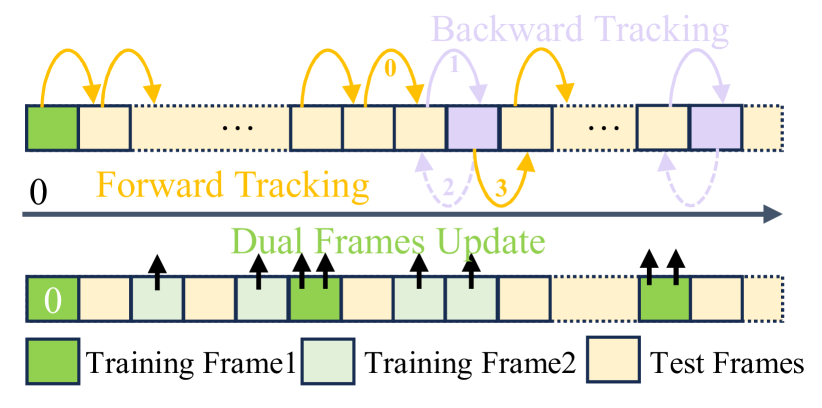
Figure 3: Overview of our proposed two online inference strategies. (1) CycleTrack (top) consists of forward and backwards tracking; (2) Dual-Frames Update (bottom) involves the update of both training frames.

III-E Online Inference

During inference, we implement two strategies to bolster tracking robustness without incurring any additional training expenses and with minimal extra inference overhead.

CycleTrack Pipeline.  During the inference stage, the existing pipeline progresses frame by frame in chronological order. While this adheres to the temporal sequence, it can encounter occasional failures or mis-tracks, particularly in the presence of distractors. In contrast, we propose a CycleTrack pipeline that rectifies the predicted candidate through backward inference if temporal cycle consistency is not satisfied, as shown in Figure 3 and Figure 4. CycleTrack hinges on the foundational principle of “temporal cycle consistency.” This signifies that a precise target candidate, when retrogressively tracked through time, should ultimately result in the localization of the current bounding box (Figure 4). The underlying hypothesis is that candidates demonstrating temporal cycle consistency are more likely to be the accurate target. In instances where there exist multiple potential target candidates, CycleTrack acts as a criterion for target selection.

The target and distractor discriminate process is formulated in Algorithm 1. Concretely, given an initial frame denoted as $\mathbf{I}^{t-1}$, our target prediction model $\mathbf{\Psi}$ is utilized to estimate the target candidate bounding box $\textbf{B}^{t}_{1}$, within the subsequent frame $\mathbf{I}^{t}$. Following that, a masking procedure is applied to this candidate region in $\mathbf{I}^{t}$, enabling the extraction of the distractor candidate $\textbf{B}^{t}_{2}$ with the succeeding maximal response. Then, we use a threshold $\tau_{c}$ as a quality measurement for $\textbf{B}^{t}_{1}$. When the classification confidence $\mathbf{S}^{t}_{1}$ is lower than $\tau_{c}$, CycleTrack will be activated. Next, we use $\mathbf{I}^{t}$ as the previous test frame and consider $\mathbf{I}^{t-1}$ as the next test frame to achieve the backward track. Based on the center and scale of $\textbf{B}^{t}_{1}$ in $\mathbf{I}^{t}$, we resize the frame $\mathbf{I}^{t-1}$ accordingly and get the model predicted candidate results $\mathbf{\hat{B}}^{t-1}_{1}$. Similarly, based on $\textbf{B}^{t}_{2}$, we generate the $\mathbf{\hat{B}}^{t-1}_{2}$. By comparing these two backward-track results, we choose the more successful backward-track input as the correct forward-track result $\textbf{B}^{t}_{1}$.

Dual-Frames Update.  In AViTMP, we employ two training frames and one test frame for joint encoding, therefore, we will search for two frames which contains the bounding box as the reference to find the target location in the test frame. During the inference phase, our approach involves using the initial frame with an annotated bounding box as the initial first training frame. The second training frame is initialized as a zero vector and then updated following the strategy introduced in ToMP [38]. Specifically, the second training frame is updated with the most recent frame when its classifier confidence surpasses a predefined threshold $\tau_{1}$. However, unlike existing methods that overlook the need for updating the first training frame in response to significant changes in the target’s scale, our approach addresses this issue. We incorporate updates to the initial training frame when detecting substantial scale changes using a high confidence threshold denoted as $\tau_{2}$.

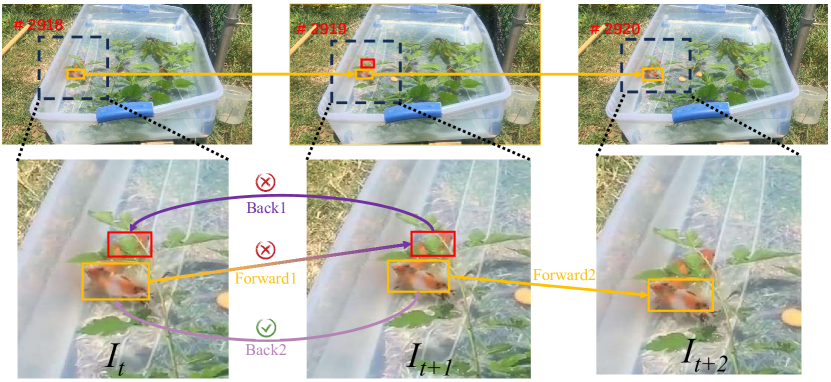
Figure 4: Detailed process of CycleTrack inference strategy. In frame #2919, the forward tracking predicts an error distractor (in red bbox) and CycleTrack corrects it to the target (in orange bbox).

Algorithm 1 CycleTrack Inference Pipeline.

Input: A sequence $\mathcal{I}=[\mathbf{I}^{1},...,\mathbf{I}^{n}]$, our target predictor $\mathbf{\Psi}$, a threshold $\tau_{c}=0.5$
For $t=1,\dots,n$ do

  # the top and sub-top predicted bbox and score.

  $(\mathbf{B}^{t}_{1},\mathbf{S}^{t}_{1}),(\mathbf{B}^{t}_{2},\mathbf{S}^{t}_{2})\leftarrow\mathbf{\Psi}(\mathbf{I}^{t},\mathbf{B}^{t-1}_{1})$

  IF $\mathbf{S}^{t}_{1}<\tau_{c}$ then $\triangleright$ Activate CycleTrack at $\mathbf{I}^{t}$

      $(\mathbf{\hat{B}}^{t-1}_{1},\mathbf{\hat{S}}^{t-1}_{1})\leftarrow\mathbf{\Psi}(\mathbf{I}^{t-1},\mathbf{B}^{t}_{1})$ $\triangleright$ Back track at $\mathbf{B}^{t}_{1}$

      $(\mathbf{\hat{B}}^{t-1}_{2},\mathbf{\hat{S}}^{t-1}_{2})\leftarrow\mathbf{\Psi}(\mathbf{I}^{t-1},\mathbf{B}^{t}_{2})$ $\triangleright$ Back track at $\mathbf{B}^{t}_{2}$

      IF $\text{IOU}(\mathbf{\hat{B}}^{t-1}_{2},\mathbf{B}^{t-1}_{1})>\text{IOU}(\mathbf{\hat{B}}^{t-1}_{1},\mathbf{B}^{t-1}_{1})$

      & $\mathbf{\hat{S}}^{t-1}_{2}>\tau_{c}$ then $\triangleright$ Correct the error prediction

           $(\mathbf{B}^{t}_{1},\mathbf{S}^{t}_{1})\leftarrow(\mathbf{B}^{t}_{2},\mathbf{S}^{t}_{2})$

Output: $\mathcal{B}=[\mathbf{B}_{1}^{1},\dots,\mathbf{B}_{1}^{n}]$

IV Experiments

IV-A Implementation Details

Training.  Our model AViTMP is implemented using the PyTracking framework [52]. The training dataset incorporates the training splits of COCO [53], LaSOT [54], GOT10k [55], and TrackingNet [56]. The training regimen comprises a total of 300 epochs, encompassing the sampling of 40,000 sub-sequences. In the mini-batch training procedure, we select $m=2$ training frames and a single test frame from a video sequence, arranging them chronologically ($x_{1}<x_{2}<x_{test}$). Consistent with recent discriminiative trackers, uniform resolution is maintained for both test and training frames. Specifically, all three frames are resized to dimensions of $288\times 288\times 3$. The patch embedding layer within ViT comprises a convolutional block, projecting frames into patch sequences of size $18\times 18\times 768$. Subsequent encoding operations ensure a consistent dimensionality between input and output features. Consequently, both the decoder and the head sections maintain a default value of $C=768$. Regarding the vanilla ViT network, we initialize the pre-trained model using unsupervised model MAE [57], while the remaining modules are trained from the ground up. The learning rate undergoes decay by a factor of 0.2 after 150 and 250 epochs. The optimization is carried out using the AdamW optimizer [58], facilitated by 4 NVIDIA A40 GPUs. To ensure the consistency of training state-prior information and the uniformity of prior distribution throughout training and testing, center and scale jitters are deliberately excluded during the training phase. Finally, our AViTMP runs at 40 FPS (Frame Per Second) on an A40 GPU.

Inference.  The hyperparameter involved in our CycleTrack process is the threshold $\tau_{c}$, which is set to 0.5. $\tau_{c}$ serves a dual purpose: it functions as the activation threshold for initiating the CycleTrack pipeline and simultaneously acts as the threshold for rectifying erroneous output results stemming from the network predictions. Regarding the training-frames update method, the subsequent training frames follow the ToMP [38] procedure, with the update threshold established at $\tau_{1}=0.85$. In relation to the initial training frames, updates are triggered under two conditions: if the predicted classifier’s confidence surpasses $\tau_{2}=0.99$, and if the target size experiences a change exceeding 16 times in comparison to the initial training frame (in terms of zooming in or out). The role of $\tau_{2}$ is to prevent inadvertent updates involving distractors during the training frames update process.

IV-B Comparison to the State of the Art

In this section, we evaluate our proposed tracker on six long-time, large-scale benchmarks, including LaSOT, LaSOTExtSub, AVisT, VOT2020, UAV123 and TNL2k. We report our tracking performance with current state-of-the-art trackers with a fair comparison.

Results on LaSOT [54]:  LaSOT is a large-scale long-term dataset composing of 280 test videos with 2500 frames on average. Table I presents the evaluations of trackers in terms of area-under-the-curve (AUC), precision, and normalized precision. Our method AViTMP showcases superior performance over recent discriminative trackers such as ToMP [38] and KeepTrack [37], boasting a substantial performance gap. It is worth highlighting that in comparison to contemporary single-branch approaches (i.e., SeqTrack-B256 [20], MixFormer [21], and OSTrack256 [23]) , AViTMP outperforms them by achieving a new state-of-the-art performance (AUC of 70.7%) when employing equitable comparisons, considering similar ViT backbone and image resolution. Furthermore, Table VI provides a comprehensive attribute-based analysis compared to the recent state-of-the-art. Notably, AViTMP exhibits a notable lead across multiple attributes, such as illumination variation, viewpoint change, fast motion, out-of-view, low resolution, and aspect ratio change. Across all 14 attributes, AViTMP secures 9 first-best results and 5 second-best results, affirming its widespread efficacy.

	Ours	MixFormer	SeqTrack		Sim	OSTrack	ToMP	ToMP	STARK	Keep	STARK	Alpha		Siam	Tr	Super	Pr
		22k	B256	GRM	-B/16	256	101	50	ST101	Track	ST50	Refine	TransT	R-CNN	DiMP	DiMP	DiMP
		[21]	[20]	[39]	[19]	[23]	[38]	[38]	[18]	[37]	[18]	[59]	[16]	[60]	[35]	[52]	[36]
Success (AUC)	70.7	70.1	69.9	69.9	69.3	69.1	68.5	67.6	67.1	67.1	66.4	65.3	64.9	64.8	63.9	63.1	59.8
Norm. Prec	80.5	78.7	79.7	79.3	78.5	78.7	78.7	78.0	76.9	77.2	76.3	73.2	73.8	72.2	73.0	72.2	68.8
Precision	75.9	74.7	76.3	75.8	75.2	-	73.5	72.2	72.2	70.2	71.2	68.0	69.0	68.4	66.3	65.3	60.8

TABLE I: Comparison on the LaSOT [54] test set ordered by AUC.

	Ours	SeqTrack	SwinTrack	Keep	OSTrack	AiA	ToMP	ToMP	LTMU		SiamRPN		Auto
		B256	B384	Track	256	Track	101	50	DiMP	DiMP	++	ATOM	Match
		[20]	[61]	[37]	[23]	[38]	[34]	[38]	[43]	[10]	[31]	[12]	[62]
Success (AUC)	50.2	49.5	49.1	48.2	47.4	46.8	45.9	45.4	41.4	39.2	34.0	37.6	37.6
Norm. Prec	62.6	60.8	-	61.7	57.3	54.4	58.1	57.6	49.9	47.6	41.6	45.9	-
Precision	57.7	56.3	55.6	54.5	53.3	54.2	52.7	51.9	47.3	45.1	39.6	43.0	43.0

TABLE II: Comparison on the LaSOTExtSub [63] test set ordered by AUC.

			MixFormer	ToMP	STARK	ToMP		Keep	Alpha	Tr	Pr
	Ours	GRM	22k	50	ST50	101	RTS	Track	Refine	DiMP	DiMP	DiMP	Ocean	ATOM
		[39]	[21]	[38]	[18]	[38]	[64]	[37]	[59]	[35]	[36]	[10]	[65]	[12]
Success (AUC)	54.9	54.5	53.7	51.6	51.1	50.9	50.8	49.4	49.6	48.1	43.3	41.9	38.9	38.6
OP50	64.0	63.1	63.0	59.5	59.2	58.8	55.7	56.3	55.7	55.3	48.0	45.7	43.6	41.5

TABLE III: Comparison on the AVisT [66] test set ordered by AUC.

	Ours	SeqTrack	ToMP	STARK	Super	CSWin	STARK	ToMP	Tr
		B256	101	ST50	DiMP	TT	ST101	50	DiMP	DPMT	TRAT	UPDT	DiMP	ATOM
		[20]	[38]	[18]	[52, 67]	[68]	[18]	[38]	[35]	[67]	[67]	[69, 67]	[10, 67]	[12, 67]
EAO	0.314	0.312	0.309	0.308	0.305	0.304	0.303	0.303	0.300	0.297	0.280	0.278	0.274	0.271
Accuracy	0.446	0.473	0.453	0.478.	0.477	0.480	0.481	0.453	0.471	0.492	0.464	0.465	0.457	0.462
Robustness	0.840	0.806	0.814	0.799	0.728	0.787	0.775	0.789	0.782	0.745	0.744	0.755	0.734	0.734

TABLE IV: Comparison to bounding box only methods on the VOT2020 [67] dataset in terms of EAO score.

		SeqTrack	Keep	OSTrack		STARK	STARK	Tr	Super	Pr	STM		Siam
	Ours	B256	Track	256	TransT	ST50	ST101	DiMP	DiMP	DiMP	Track	Ocean	R-CNN	KYS	DiMP
		[20]	[37]	[23]	[16]	[18]	[18]	[35]	[52]	[36]	[70]	[65]	[60]	[11]	[10]
UAV123	70.1	69.2	69.7	68.3	69.1	69.1	68.2	67.5	67.7	68.0	64.7	57.4	64.9	-	65.3
TNL2k	54.5	54.9	-	54.3	50.7	-	-	-	49.2	47.0	38.4	-	52.3	44.9	44.7

TABLE V: Comparison with the state-of-the-art methods on UAV123 [71] and TNL2k [72] in terms of AUC.

	Illumination	Partial		Motion	Camera		Background	Viewpoint	Scale	Full	Fast		Low	Aspect
	Variation	Occlusion	Deformation	Blur	Motion	Rotation	Clutter	Change	Variation	Occlusion	Motion	Out-of-View	Resolution	Ration Change	Total
TransT	65.2	62.0	67.0	63.0	67.2	64.3	57.9	61.7	64.6	55.3	51.0	58.2	56.4	63.2	64.9
STARK-ST101	67.5	65.1	68.3	64.5	69.5	66.6	57.4	68.8	66.8	58.9	54.2	63.3	59.6	65.6	67.1
KeepTrack	69.7	64.1	67.0	66.7	71.0	65.3	61.2	66.9	66.8	60.1	57.7	64.1	62.0	65.9	67.1
ToMP-50	66.8	64.9	68.5	64.6	70.2	67.3	59.1	67.2	67.5	59.3	56.1	63.7	61.1	66.5	67.6
ToMP-101	69.0	65.3	69.4	65.2	71.7	67.8	61.5	69.2	68.4	59.1	57.9	64.1	62.5	67.2	68.5
OSTrack256	68.7	66.6	71.2	66.4	72.0	68.6	61.5	69.1	69.0	59.5	55.7	63.2	61.7	67.4	69.1
MixFormer22k	69.6	66.5	69.7	66.5	71.6	68.6	59.9	70.6	68.9	61.4	56.6	64.4	62.9	67.7	70.1
GRM	70.0	67.9	72.3	66.7	71.9	69.3	62.1	68.4	69.8	60.8	55.3	64.5	62.5	68.2	69.9
SeqTrack-B256	68.6	67.7	70.8	69.2	73.3	69.8	62.9	71.3	69.6	61.6	57.8	64.6	62.2	68.3	69.9
Ours	71.5	67.8	71.7	66.8	73.2	70.4	62.8	73.2	70.3	63.3	59.8	66.8	64.8	69.3	70.7

TABLE VI: The comparison of different attributes analysis with the state-of-the-art on LaSOT [54] benchmark.

Results on LaSOTExtSub [63]:  LaSOTExtSub is an extension of LaSOT dataset. It contains 15 new classes with 150 test sequences in total. LaSOTExtSub also encompasses lots of long-term sequences with distractor scenarios. As shown in Table II, under the conditions of aligned settings, AViTMP attains a novel state-of-the-art performance at 50.2% AUC, surpassing the discriminative tracker ToMP101 by a significant margin of 4.3%. When considering an equivalent ViT-B backbone and similar resolution, we also outperform the single-branch tracker SeqTrack-B256 by 0.7% in terms of AUC.

Results on AVisT [66]:  AVisT is a recently released benchmark, which comprises 120 sequences in a variety of adverse scenarios highly relevant to real-world applications, such as bad weather conditions and camouflage. As shown in Table III, under the fair comparison situation, our tracker outperforms the other trackers, including GRM and MixFormer-22k, setting a new state-of-the-art AUC score under challenging scenarios.

Results on VOT2020_Bbox [67]:  VOT2020 contains 60 videos and we compare the top methods in VOT challenge [67]. Instead of the one-pass evaluation, the trackers are evaluated following the multi-start protocol which is specifically suited for the VOT challenge. Since AViTMP is supervised by bounding boxes solely, we compare the bounding box trackers in Table IV. Our approach performs better compared with SeqTrack-B256, CSWinTT, and ToMP101 in overall performance. Especially AViTMP achieves 0.840 in robustness attribute, outperforming SeqTrack-B256 and ToMP101 with 3.4% and 2.6% respectively. In the multi-start protocol, the quality of the initial frame is hard to predict, making the evaluation results much closer to a real application. The robustness performance (tracking failure times) comparison shows the powerful effectiveness of our inference strategies in contributing to the robustness of tracking. Figure 5 displays the ranking of trackers based on EAO for clear representation. Notably, AViTMP stands out as the top-performing tracker in this evaluation.

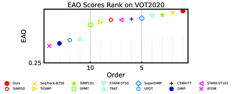
Figure 5: EAO ranking on VOT2020_Bbox dataset.

Results on UAV123 [71]:  UAV123 is a UAV dataset with 123 test videos mainly containing fast motion, small targets and distractors. It is over 1200 frames on average in a video. Table V shows that AViTMP achieves a 70.1% AUC score, outperforming the previous distractor inhibition two-branch discriminate method KeepTrack.

Results on TNL2k [72]:  TNL2k is a large-scale and recently dataset with 700 sequences. Table V also reports the results following the bounding-box guided tracking rule, AViTMP achieves 54.5% AUC, competitive with SeqTrack-B256 and OSTrack-256.

IV-C Evaluation on Other Datasets

We extend the evaluation to encompass datasets such as VOT2020_mask [67], TrackingNet [56], OTB100 [73], and NFS30 [74] for extensive comparison.

TrackingNet.  TrackingNet [56] encompasses a collection of over 30,000 training videos, adopting a labelling strategy with a 30-frame interval. In contrast to datasets like LaSOT, LaSOTExtSub, etc. which are long-time datasets, TrackingNet is positioned as a middle-time dataset (around 500 frames for each video) and is relatively less challenging in terms of long-term tracking attributes such as fast motion, distractors, and out-of-view scenarios. The outcomes presented in Table VII indicate that our tracker achieves an AUC of 82.8%, positioning it comparably with the current state-of-the-art trackers SeqTrack-B256 and MixFormer-1k, which are concentrating on feature extraction and representation capabilities.

VOT2020_Mask.  In contrast to previous years, where sequences in the VOT challenge were annotated with bounding boxes [75, 76], the recent challenge now incorporates evaluation based on segmentation masks in each frame. We additionally evaluate our method in VOT2020 under the segmentation situation. For this evaluation, after AViTMP predicted the bounding box of the target, we employed the image segmentation method HQ-SAM [77] to generate the required masks. As highlighted in Table VIII, our tracker attains an EAO of 0.504, coupled with a robustness performance of 0.821. With the tracking combined with the segmentation pipeline, accuracy performance heavily depends on the quality of segmentation methods and the robustness mainly depends on the tracking method. These comparison outcomes further underscore the robust performance achieved by our AViTMP.

OTB100.  We extend our reporting to include results from the OTB100 [73] dataset, featuring 100 short sequences. On this renowned and nearly saturated dataset, we attain scores of 70.3, 90.6, and 84.5 for AUC, precision (PRE), and normalized precision rate (NPR), respectively. Table IX outlines the success rate comparison with prior trackers, demonstrating that the majority of them hover around the $70\pm 2\%$ range.

NFS30.  NFS30 [74] stands as a compact and short-term classical dataset. Our performance on this dataset is highlighted in Table X, where we achieve an AUC of 66.3%. This result positions us competitively among contemporary state-of-the-art trackers.

	Ours	SeqTrack	MixFormer	ToMP	STARK		STARK	Siam	Alpha	STM	Tr	Keep	Super	Pr
		B256	-1k	101	ST101	TransT	ST50	R-CNN	Refine	Track	DiMP	Track	DiMP	DiMP
		[20]	[21]	[38]	[18]	[16]	[18]	[60]	[59]	[70]	[35]	[37]	[52]	[36]
PRE	80.7	82.2	81.2	78.9	-	80.3	-	80.0	78.3	76.7	73.1	73.8	73.3	70.4
NPR	87.1	88.3	87.7	86.4	86.9	86.7	86.1	85.4	85.6	85.1	83.3	83.5	83.5	81.6
AUC	82.8	83.3	82.6	81.5	82.0	81.4	81.3	81.2	80.5	80.3	78.4	78.1	78.1	75.8

TABLE VII: Comparison with other method on the TrackingNet [56] test set.

		ToMP	ToMP	SeqTrack	STARK	STARK	Ocean	Alpha
	Ours	101+AR	50 +AR	B256+AR	ST50+AR	ST101+AR	Plus	Refine	AFOD	LWTL
		[38]	[38]	[67]	[18]	[18]	[67]	[59, 67]	[67]	[67]
EAO	0.504	0.497	0.496	0.520	0.505	0.497	0.491	0.482	0.472	0.463
A	0.725	0.750	0.754	-	0.759	0.763	0.685	0.754	0.713	0.719
R	0.821	0.798	0.793	-	0.817	0.789	0.842	0.777	0.795	0.798

TABLE VIII: Comparison to segmentation only methods on VOT2020 [67] in terms of EAO score.

AiA

ToMP

Keep

STARK

Tr

STARK

Super

Pr

Siam

STM

Ours

Track

101

Track

ST101

DiMP

TransT

ST50

DiMP

DiMP

R-CNN

Track

DiMP

[34]

[38]

[37]

[18]

[35]

[16]

[18]

[52]

[36]

[60]

[70]

[10]

AUC

70.3

69.6

70.1

70.9

68.1

71.1

69.4

71.4

70.1

69.6

70.1

71.9

68.4

TABLE IX: Comparison with state-of-the-art on the OTB-100 [73] datasets in terms of overall AUC score.

SeqTrack

Keep

OSTrack

STARK

STARK

Tr

Super

Pr

STM

Siam

Ours

GRM

B256

Track

256

TransT

ST50

ST101

DiMP

DiMP

DiMP

Track

R-CNN

[39]

[20]

[37]

[23]

[16]

[18]

[18]

[35]

[52]

[36]

[70]

[60]

NFS30

66.3

65.6

67.6

66.4

64.7

65.7

65.2

66.2

66.5

64.8

63.5

49.4

63.9

TABLE X: Comparison with the state-of-the-art methods on NFS30 [74] in terms of AUC.

IV-D Visualization Analysis

Frames Visualization.  Figure 6 illustrates several frames from six distinct LaSOT sequences, each containing both ground truth and predicted bounding boxes. In the first row, our tracker shows precise predictions, primarily attributed to our novel update inference means. Specifically, a substantial change in scale occurs between the initial frame and the #1144 frame, leading to considerable degradation of the initial frame’s predictive capability, as it advances through subsequent frames. This phenomenon results in imprecise predictions and bounding boxes that inadequately encompass the target area in subsequent frames (#1144, #1395, and #1615). The subsequent five rows highlight the tracker’s robustness against the challenge of resembling distractors. Compared with AViTMP, other trackers are all based on the feature matching of template and search, which is easily failed by extremely similar distractors with a lack of location temporal consistency along adjacent frames (i.e., tigers in row 5th). Particularly, in the third row, AViTMP adeptly counteracts the impact of distractors even in heavy occlusion scenarios (#1285 and #3156).

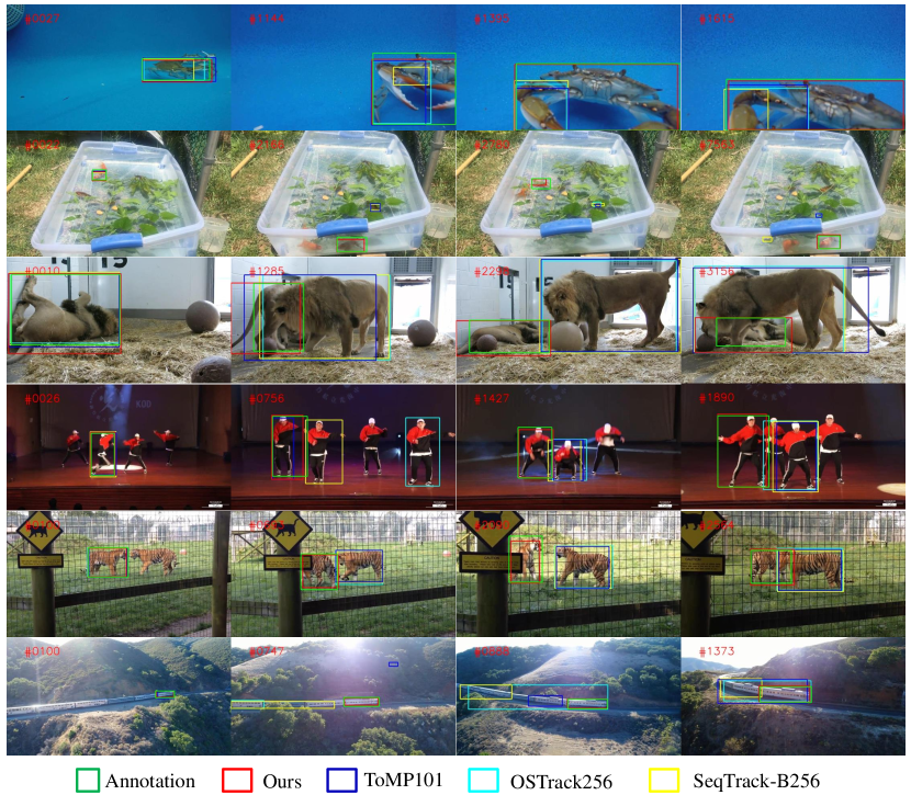
Figure 6: Tracking results visualization of different trackers.

Futures Visualization.  With consistent dimensions of the encoder component features, the decoder component can receive inputs either from the adaptor or the ViT feature. Within our framework, the output feature from the adaptor, rather than ViT, is utilized as the input for the subsequent decoder modules. To qualitatively compare the distribution of AViT-Enc features, we present an overall and each layer visualization of the output features from both the AViT-Enc components.

When comparing the output feature in the last column of Figure 7, we observe that the feature map of adaptor output exhibits a more precise concentration on the target, while the ViT feature yields a more extensive feature representation. Figure 7 also presents a qualitative comparison of layer-wise features between ViT and the Adaptor to substantiate their distinctions in feature distribution. During the testing phase, the test frame undergoes resizing and padding using nearby pixels. Upon closer examination of the results, it becomes evident that different layers of the Adaptor tend to concentrate on distinct regions of the test frame. Specifically, layers 1 to 11 within the adaptor exhibit a relatively weak association with the target’s shape and instead concentrate on various regions of interest independently. In the ViT row, the features of each ViT layer appear remarkably consistent, except the last layer. Across layers 1 to 11, there is a notable concentration of high response in the central region, while the response gradually diminishes in the bottom-right region as we move through the layers. This observation leads us to assert that various layers of ViT exhibit attention towards a similar region. In contrast, our Adaptor showcases varying regions of concern as we delve deeper into the layer structure. Analyzing the last layer’s features, it becomes evident that the final Adaptor feature concentrates more intently on the target region, whereas the ViT feature is susceptible to being influenced by the background. This analysis yields two noteworthy conclusions: 1) Adaptor and ViT exhibit distinct feature distributions, emphasizing different aspects apart from the last layer; 2) In the last layer’s feature, the Adaptor module is responsive to precise target-related regions, a contrast to the broader feature focus of ViT.

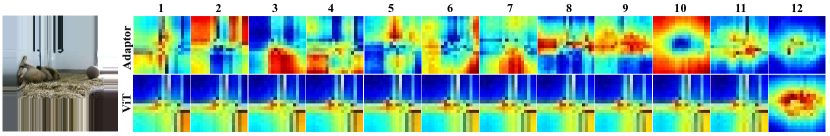
Figure 7: Feature visualization of each layer in AViT Encoder.

Attributes Visualization.  For a more detailed perspective, Figure 8 offers 12 attribute-specific success curves compared to these state-of-the-art methods. Our method performs especially well when the overlap threshold is less than 0.6. Especially, our tracker performs much better on Full Occlusion (+1.5), Illumination Variation (+1.5), Viewpoint Change (+1.9), Fast Motion (+1.9), Low Resolution (+1.9), and Out-of-view (+2.2) compared with the second best. Through the comprehensive visual analysis, we assert that our method AViTMP attains a state-of-the-art performance across many attributes in the context of long-term tracking.

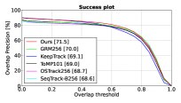
((a))

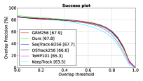
((b))

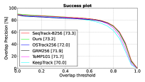
((c))

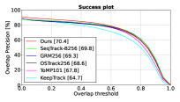
((d))

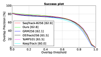
((e))

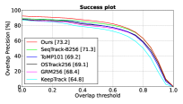
((f))

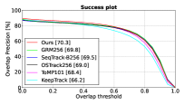
((g))

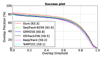
((h))

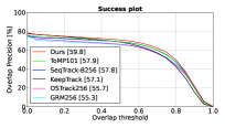
((i))

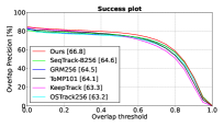
((j))

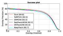
((k))

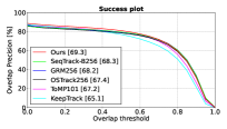
((l))

Figure 8: Attributes success rate visualization comparison of state-of-the-art methods on LaSOT [54] benchmark.

IV-E Ablation and Analysis

Network Architecture.  In order to analyse the effect of AViT-Enc and DF-Dec, we train different variants of the encoder and decoder to ablate their role. As shown in Table XI, we report results for three variants encoders and two decoder parts. As we can observe, the vanilla ViT encoder (#1) without the adaptor and joint state embedding sets the lowest performance in these encoder variants. In #2 row, as we employ the joint state embedding for each ViT layer, AUC improves 1.4%/0.8% in LaSOT and LaSOTExtSub respectively. While only embedding the adaptor module (#3 row), AUC outperforms the baseline with 3.4%/2.7%, showing the effectiveness and powerful ability of the adaptor in contributing to AViT-Enc. Finally, after combing the JSE and Adaptor together (#5 row) to build our AViT-Enc, we achieved the best performance compared with the vanilla ViT encoder. Additionally, #4 shows the ablation of our dense-fusion decoder. After replacing DF-Dec with a standard decoder  [32], AUC scores decrease around 4.7%/2.0% compared with DF-Dec (#5).

#	JSE	Adaptor	DF-Dec	S-Dec	LaSOT	$\Delta_{1}$	LaSOTExtSub	$\Delta_{2}$
1			✓		65.7	-	45.8	-
2	✓		✓		67.1	+1.4	46.6	+0.8
3		✓	✓		69.1	+3.4	48.5	+2.7
4	✓	✓		✓	70.4	+4.7	47.8	+2.0
5	✓	✓	✓		70.7	+5.0	50.2	+4.4

TABLE XI: Analysis of architecture component variants. S-Dec denotes the plain standard decoder [32]. $\Delta$ denotes the AUC change compared with the baseline (1st row).

#	CycleTrack	Dual-Frame Update	LaSOT	$\Delta_{1}$	LaSOTExtSub	$\Delta_{2}$	FPS
1			68.0	-	48.2	-	42
2	✓		68.9	+0.9	48.7	+0.5	41
3		✓	70.1	+2.1	49.7	+1.5	40
4	✓	✓	70.7	+2.7	50.2	+2.0	40

TABLE XII: Ablation on LaSOT and LaSOTExtSub over inference strategies. $\Delta$ denotes the AUC change compared with the baseline (1st row). FPS measures the inference speed.

Inference Strategies. During inference, we assess the effectiveness of our strategies in Table XII. Upon the introduction of CycleTrack (#2), AUC improves by 0.7% on average with virtually no additional inference cost and speed influence (-1 FPS). By updating the two training frames during inference (#3), AUC improves by 2.1%/1.5% with only 2 FPS speed cost, which proves particularly effective in long-term tracking, especially with obviously scale-fluctuation, deformation, and poor-quality initial frame situations. Consequently, we assert that the strategy of updating dual frames is beneficial for enhancing robustness in long-term tracking. Finally, with the amalgamation of these two strategies, AViTMP surpasses our base with 2.7%/2.0%, while incurring a minimal cost of 2 FPS. As shown in Figure 4, CycleTrack effectively rectifies erroneous predictions based on the temporal cycle consistency under distractor scenarios.

Tracking Speed.  As shown in Table XIII, our method achieves around 40 FPS, comparable with previous single-branch network SeqTrack-B256 and GRM. Compared with the discriminate trackers ToMP and KeepTrack, our inference speed is much faster. This confirms that our method not only combines the benefit of single-branch and discriminate trackers, and does so with a fast running speed.

TABLE XIII: Tracking speed report of various trackers. We have reported the numbers and GPU-type provided by the authors. The best results are shown in bold.

	ToMP101	KeepTrack	GRM	MixFormer-22k	SeqTrack-B256	Ours
FPS	20	18	45	25	40	40
GPU	2080Ti	2080Ti	RTX3090	1080Ti	2080Ti	A40

V Conclusion

In this paper, we introduce a novel model, AViTMP, which operates as an adaptive Vision Transformer model predictor for single-branch visual tracking. By employing a rich-prior embedding, AViTMP encodes target features and estimates model weights to predict object locations in test frames. With the integration of the AViT Encoder and discriminate model prediction, we seamlessly combine the advantages of discriminative models with those of single-branch trackers, establishing a cutting-edge paradigm in visual tracking. Moreover, our focus extends to refining the inference process, yielding the CycleTrack and dual-frame update strategies to ensure the integration of temporal consistency and robustness inference within sequences. Comprehensive experiments and analyses validate the effectiveness of our proposed method. As a result, we establish state-of-the-art performance across various benchmarks. In future works, we will consider extending the temporal consistency strategy into other tracking algorithms and also explore more effective and efficient inference methods to improve the robustness tracking ability in complex scenarios without additional network and training costs.

References

- [1] R. Wang, B. Zhong, and Y. Chen, “Motion-driven tracking via end-to-end coarse-to-fine verifying,” IEEE Transactions on Circuits and Systems for Video Technology, pp. 1–1, 2023.
- [2] C. Tang, Q. Hu, G. Zhou, J. Yao, J. Zhang, Y. Huang, and Q. Ye, “Transformer sub-patch matching for high-performance visual object tracking,” IEEE Transactions on Intelligent Transportation Systems, 2023.
- [3] S. Javed, M. Danelljan, F. S. Khan, M. H. Khan, M. Felsberg, and J. Matas, “Visual object tracking with discriminative filters and siamese networks: a survey and outlook,” IEEE Transactions on Pattern Analysis and Machine Intelligence, vol. 45, no. 5, pp. 6552–6574, 2022.
- [4] C. Tang, X. Wang, Y. Bai, Z. Wu, J. Zhang, and Y. Huang, “Learning spatial-frequency transformer for visual object tracking,” IEEE Transactions on Circuits and Systems for Video Technology, 2023.
- [5] X. Wang, Z. Chen, J. Tang, B. Luo, Y. Wang, Y. Tian, and F. Wu, “Dynamic attention guided multi-trajectory analysis for single object tracking,” IEEE Transactions on Circuits and Systems for Video Technology, vol. 31, no. 12, pp. 4895–4908, 2021.
- [6] J. Zhu, Y. Lao, and Y. F. Zheng, “Object tracking in structured environments for video surveillance applications,” IEEE Transactions on Circuits and Systems for Video Technology, vol. 20, no. 2, pp. 223–235, 2009.
- [7] Y. Liang, Q. Wu, Y. Liu, Y. Yan, and H. Wang, “Deep correlation filter tracking with shepherded instance-aware proposals,” IEEE Transactions on Intelligent Transportation Systems, 2021.
- [8] Y. Cao, H. Ji, W. Zhang, and S. Shirani, “Feature aggregation networks based on dual attention capsules for visual object tracking,” IEEE Transactions on Circuits and Systems for Video Technology, vol. 32, no. 2, pp. 674–689, 2021.
- [9] F. Lin, C. Fu, Y. He, F. Guo, and Q. Tang, “Learning temporary block-based bidirectional incongruity-aware correlation filters for efficient uav object tracking,” IEEE Transactions on Circuits and Systems for Video Technology, vol. 31, no. 6, pp. 2160–2174, 2020.
- [10] G. Bhat, M. Danelljan, L. V. Gool, and R. Timofte, “Learning discriminative model prediction for tracking,” in Proceedings of the IEEE/CVF international conference on computer vision, 2019, pp. 6182–6191.
- [11] G. Bhat, M. Danelljan, L. Van Gool, and R. Timofte, “Know your surroundings: Exploiting scene information for object tracking,” in European Conference on Computer Vision. Springer, 2020, pp. 205–221.
- [12] M. Danelljan, G. Bhat, F. S. Khan, and M. Felsberg, “Atom: Accurate tracking by overlap maximization,” in Proceedings of the IEEE/CVF conference on computer vision and pattern recognition, 2019, pp. 4660–4669.
- [13] M. Danelljan, G. Hager, F. Shahbaz Khan, and M. Felsberg, “Learning spatially regularized correlation filters for visual tracking,” in Proceedings of the IEEE international conference on computer vision, 2015, pp. 4310–4318.
- [14] M. Danelljan, A. Robinson, F. Shahbaz Khan, and M. Felsberg, “Beyond correlation filters: Learning continuous convolution operators for visual tracking,” in Computer Vision–ECCV 2016: 14th European Conference, Amsterdam, The Netherlands, October 11-14, 2016, Proceedings, Part V 14. Springer, 2016, pp. 472–488.
- [15] L. Bertinetto, J. Valmadre, J. F. Henriques, A. Vedaldi, and P. H. Torr, “Fully-convolutional siamese networks for object tracking,” in European Conference on Computer Vision. Springer, 2016, pp. 850–865.
- [16] X. Chen, B. Yan, J. Zhu, D. Wang, X. Yang, and H. Lu, “Transformer tracking,” in Proceedings of the IEEE/CVF Conference on Computer Vision and Pattern Recognition, 2021, pp. 8126–8135.
- [17] B. Li, J. Yan, W. Wu, Z. Zhu, and X. Hu, “High performance visual tracking with siamese region proposal network,” in Proceedings of the IEEE/CVF conference on computer vision and pattern recognition, 2018, pp. 8971–8980.
- [18] B. Yan, H. Peng, J. Fu, D. Wang, and H. Lu, “Learning spatio-temporal transformer for visual tracking,” in Proceedings of the IEEE/CVF International Conference on Computer Vision, 2021, pp. 10 448–10 457.
- [19] B. Chen, P. Li, L. Bai, L. Qiao, Q. Shen, B. Li, W. Gan, W. Wu, and W. Ouyang, “Backbone is all your need: A simplified architecture for visual object tracking,” ECCV, 2022.
- [20] X. Chen, H. Peng, D. Wang, H. Lu, and H. Hu, “Seqtrack: Sequence to sequence learning for visual object tracking,” in Proceedings of the IEEE/CVF Conference on Computer Vision and Pattern Recognition, 2023, pp. 14 572–14 581.
- [21] Y. Cui, C. Jiang, L. Wang, and G. Wu, “Mixformer: End-to-end tracking with iterative mixed attention,” in Proceedings of the IEEE/CVF Conference on Computer Vision and Pattern Recognition, 2022, pp. 13 608–13 618.
- [22] F. Xie, C. Wang, G. Wang, Y. Cao, W. Yang, and W. Zeng, “Correlation-aware deep tracking,” in Proceedings of the IEEE/CVF Conference on Computer Vision and Pattern Recognition, 2022, pp. 8751–8760.
- [23] B. Ye, H. Chang, B. Ma, and S. Shan, “Joint feature learning and relation modeling for tracking: A one-stream framework,” ECCV, 2022.
- [24] Z. Liu, Y. Lin, Y. Cao, H. Hu, Y. Wei, Z. Zhang, S. Lin, and B. Guo, “Swin transformer: Hierarchical vision transformer using shifted windows,” in Proceedings of the IEEE/CVF international conference on computer vision, 2021, pp. 10 012–10 022.
- [25] W. Wang, E. Xie, X. Li, D.-P. Fan, K. Song, D. Liang, T. Lu, P. Luo, and L. Shao, “Pyramid vision transformer: A versatile backbone for dense prediction without convolutions,” in Proceedings of the IEEE/CVF international conference on computer vision, 2021, pp. 568–578.
- [26] E. Xie, W. Wang, Z. Yu, A. Anandkumar, J. M. Alvarez, and P. Luo, “Segformer: Simple and efficient design for semantic segmentation with transformers,” Advances in Neural Information Processing Systems, vol. 34, pp. 12 077–12 090, 2021.
- [27] Z. Chen, Y. Duan, W. Wang, J. He, T. Lu, J. Dai, and Y. Qiao, “Vision transformer adapter for dense predictions,” arXiv preprint arXiv:2205.08534, 2022.
- [28] S. Javed, M. Danelljan, F. S. Khan, M. H. Khan, M. Felsberg, and J. Matas, “Visual object tracking with discriminative filters and siamese networks: a survey and outlook,” IEEE Transactions on Pattern Analysis and Machine Intelligence, vol. 45, no. 5, pp. 6552–6574, 2022.
- [29] S. M. Marvasti-Zadeh, L. Cheng, H. Ghanei-Yakhdan, and S. Kasaei, “Deep learning for visual tracking: A comprehensive survey,” IEEE Transactions on Intelligent Transportation Systems, vol. 23, no. 5, pp. 3943–3968, 2022.
- [30] Z. Chen, B. Zhong, G. Li, S. Zhang, and R. Ji, “Siamese box adaptive network for visual tracking,” in Proceedings of the IEEE/CVF conference on computer vision and pattern recognition, 2020, pp. 6668–6677.
- [31] B. Li, W. Wu, Q. Wang, F. Zhang, J. Xing, and J. Yan, “Siamrpn++: Evolution of siamese visual tracking with very deep networks,” in Proceedings of the IEEE/CVF Conference on Computer Vision and Pattern Recognition, 2019, pp. 4282–4291.
- [32] N. Carion, F. Massa, G. Synnaeve, N. Usunier, A. Kirillov, and S. Zagoruyko, “End-to-end object detection with transformers,” in European conference on computer vision. Springer, 2020, pp. 213–229.
- [33] A. Vaswani, N. Shazeer, N. Parmar, J. Uszkoreit, L. Jones, A. N. Gomez, Ł. Kaiser, and I. Polosukhin, “Attention is all you need,” Advances in neural information processing systems, vol. 30, 2017.
- [34] S. Gao, C. Zhou, C. Ma, X. Wang, and J. Yuan, “Aiatrack: Attention in attention for transformer visual tracking,” arXiv preprint arXiv:2207.09603, 2022.
- [35] N. Wang, W. Zhou, J. Wang, and H. Li, “Transformer meets tracker: Exploiting temporal context for robust visual tracking,” in Proceedings of the IEEE/CVF conference on computer vision and pattern recognition, 2021, pp. 1571–1580.
- [36] M. Danelljan, L. V. Gool, and R. Timofte, “Probabilistic regression for visual tracking,” in Proceedings of the IEEE/CVF conference on computer vision and pattern recognition, 2020, pp. 7183–7192.
- [37] C. Mayer, M. Danelljan, D. P. Paudel, and L. Van Gool, “Learning target candidate association to keep track of what not to track,” in Proceedings of the IEEE/CVF International Conference on Computer Vision, 2021, pp. 13 444–13 454.
- [38] C. Mayer, M. Danelljan, G. Bhat, M. Paul, D. P. Paudel, F. Yu, and L. Van Gool, “Transforming model prediction for tracking,” in Proceedings of the IEEE/CVF Conference on Computer Vision and Pattern Recognition, 2022, pp. 8731–8740.
- [39] S. Gao, C. Zhou, and J. Zhang, “Generalized relation modeling for transformer tracking,” in Proceedings of the IEEE/CVF Conference on Computer Vision and Pattern Recognition, 2023, pp. 18 686–18 695.
- [40] A. Dosovitskiy, L. Beyer, A. Kolesnikov, D. Weissenborn, X. Zhai, T. Unterthiner, M. Dehghani, M. Minderer, G. Heigold, S. Gelly et al., “An image is worth 16x16 words: Transformers for image recognition at scale,” arXiv preprint arXiv:2010.11929, 2020.
- [41] H. Wu, B. Xiao, N. Codella, M. Liu, X. Dai, L. Yuan, and L. Zhang, “Cvt: Introducing convolutions to vision transformers,” in Proceedings of the IEEE/CVF international conference on computer vision, 2021, pp. 22–31.
- [42] J. F. Henriques, R. Caseiro, P. Martins, and J. Batista, “High-speed tracking with kernelized correlation filters,” IEEE Transactions on pattern analysis and machine intelligence, vol. 37, no. 3, pp. 583–596, 2014.
- [43] K. Dai, Y. Zhang, D. Wang, J. Li, H. Lu, and X. Yang, “High-performance long-term tracking with meta-updater,” in Proceedings of the IEEE/CVF Conference on Computer Vision and Pattern Recognition, 2020, pp. 6298–6307.
- [44] L. Zhang, A. Gonzalez-Garcia, J. V. D. Weijer, M. Danelljan, and F. S. Khan, “Learning the model update for siamese trackers,” in Proceedings of the IEEE/CVF international conference on computer vision, 2019, pp. 4010–4019.
- [45] B. Jiang, R. Luo, J. Mao, T. Xiao, and Y. Jiang, “Acquisition of localization confidence for accurate object detection,” in Proceedings of the European conference on computer vision (ECCV), 2018, pp. 784–799.
- [46] K. Dai, D. Wang, H. Lu, C. Sun, and J. Li, “Visual tracking via adaptive spatially-regularized correlation filters,” in Proceedings of the IEEE/CVF Conference on Computer Vision and Pattern Recognition, 2019, pp. 4670–4679.
- [47] L. Zheng, M. Tang, Y. Chen, J. Wang, and H. Lu, “Learning feature embeddings for discriminant model based tracking,” in Computer Vision–ECCV 2020: 16th European Conference, Glasgow, UK, August 23–28, 2020, Proceedings, Part XV 16. Springer, 2020, pp. 759–775.
- [48] T. M. Nguyen, T. M. Nguyen, N. Ho, A. L. Bertozzi, R. Baraniuk, and S. Osher, “A primal-dual framework for transformers and neural networks,” in The Eleventh International Conference on Learning Representations, 2022.
- [49] H. Nt and T. Maehara, “Revisiting graph neural networks: All we have is low-pass filters,” arXiv preprint arXiv:1905.09550, 2019.
- [50] C. Cai and Y. Wang, “A note on over-smoothing for graph neural networks,” arXiv preprint arXiv:2006.13318, 2020.
- [51] H. Rezatofighi, N. Tsoi, J. Gwak, A. Sadeghian, I. Reid, and S. Savarese, “Generalized intersection over union: A metric and a loss for bounding box regression,” in Proceedings of the IEEE/CVF Conference on Computer Vision and Pattern Recognition (CVPR), June 2019.
- [52] M. Danelljan and G. Bhat, “PyTracking: Visual tracking library based on PyTorch.” https://github.com/visionml/pytracking, 2019, accessed: 1/05/2021.
- [53] T.-Y. Lin, M. Maire, S. Belongie, J. Hays, P. Perona, D. Ramanan, P. Dollár, and C. L. Zitnick, “Microsoft coco: Common objects in context,” in European Conference on Computer Vision. Springer, 2014, pp. 740–755.
- [54] H. Fan, L. Lin, F. Yang, P. Chu, G. Deng, S. Yu, H. Bai, Y. Xu, C. Liao, and H. Ling, “Lasot: A high-quality benchmark for large-scale single object tracking,” in Proceedings of the IEEE/CVF conference on computer vision and pattern recognition, 2019, pp. 5374–5383.
- [55] L. Huang, X. Zhao, and K. Huang, “Got-10k: A large high-diversity benchmark for generic object tracking in the wild,” IEEE Transactions on Pattern Analysis and Machine Intelligence, 2019.
- [56] M. Muller, A. Bibi, S. Giancola, S. Alsubaihi, and B. Ghanem, “Trackingnet: A large-scale dataset and benchmark for object tracking in the wild,” in European Conference on Computer Vision, 2018, pp. 300–317.
- [57] K. He, X. Chen, S. Xie, Y. Li, P. Dollár, and R. Girshick, “Masked autoencoders are scalable vision learners,” in Proceedings of the IEEE/CVF conference on computer vision and pattern recognition, 2022, pp. 16 000–16 009.
- [58] I. Loshchilov and F. Hutter, “Decoupled weight decay regularization,” arXiv preprint arXiv:1711.05101, 2017.
- [59] B. Yan, X. Zhang, D. Wang, H. Lu, and X. Yang, “Alpha-refine: Boosting tracking performance by precise bounding box estimation,” in Proceedings of the IEEE/CVF Conference on Computer Vision and Pattern Recognition (CVPR), June 2021.
- [60] P. Voigtlaender, J. Luiten, P. H. Torr, and B. Leibe, “Siam r-cnn: Visual tracking by re-detection,” in Proceedings of the IEEE/CVF conference on computer vision and pattern recognition, 2020, pp. 6578–6588.
- [61] L. Lin, H. Fan, Y. Xu, and H. Ling, “Swintrack: A simple and strong baseline for transformer tracking,” arXiv preprint arXiv:2112.00995, 2021.
- [62] Z. Zhang, Y. Liu, X. Wang, B. Li, and W. Hu, “Learn to match: Automatic matching network design for visual tracking,” in Proceedings of the IEEE international conference on computer vision, 2021, pp. 13 339–13 348.
- [63] H. Fan, H. Bai, L. Lin, F. Yang, P. Chu, G. Deng, S. Yu, M. Huang, J. Liu, Y. Xu et al., “Lasot: A high-quality large-scale single object tracking benchmark,” International Journal of Computer Vision (IJCV), vol. 129, no. 2, pp. 439–461, 2021.
- [64] M. Paul, M. Danelljan, C. Mayer, and L. Van Gool, “Robust visual tracking by segmentation,” arXiv preprint arXiv:2203.11191, 2022.
- [65] Z. Zhang, H. Peng, J. Fu, B. Li, and W. Hu, “Ocean: Object-aware anchor-free tracking,” in Computer Vision–ECCV 2020: 16th European Conference, Glasgow, UK, August 23–28, 2020, Proceedings, Part XXI 16. Springer, 2020, pp. 771–787.
- [66] M. Noman, W. A. Ghallabi, D. Najiha, C. Mayer, A. Dudhane, M. Danelljan, H. Cholakkal, S. Khan, L. Van Gool, and F. S. Khan, “Avist: A benchmark for visual object tracking in adverse visibility,” arXiv preprint arXiv:2208.06888, 2022.
- [67] M. Kristan, A. Leonardis, J. Matas, M. Felsberg, R. Pflugfelder, J.-K. Kämäräinen, M. Danelljan, L. Č. Zajc, A. Lukežič, O. Drbohlav, L. He, Y. Zhang, S. Yan, J. Yang, G. Fernández, and et al, “The eighth visual object tracking vot2020 challenge results,” in Proceedings of the European Conference on Computer Vision Workshops (ECCVW), August 2020.
- [68] Z. Song, J. Yu, Y.-P. P. Chen, and W. Yang, “Transformer tracking with cyclic shifting window attention,” in Proceedings of the IEEE/CVF Conference on Computer Vision and Pattern Recognition, 2022, pp. 8791–8800.
- [69] G. Bhat, J. Johnander, M. Danelljan, F. S. Khan, and M. Felsberg, “Unveiling the power of deep tracking,” in Proceedings of the European Conference on Computer Vision (ECCV), September 2018.
- [70] Z. Fu, Q. Liu, Z. Fu, and Y. Wang, “Stmtrack: Template-free visual tracking with space-time memory networks,” in Proceedings of the IEEE/CVF conference on computer vision and pattern recognition, 2021, pp. 13 774–13 783.
- [71] M. Mueller, N. Smith, and B. Ghanem, “A benchmark and simulator for uav tracking,” in Proceedings of the European Conference on Computer Vision (ECCV), October 2016.
- [72] X. Wang, X. Shu, Z. Zhang, B. Jiang, Y. Wang, Y. Tian, and F. Wu, “Towards more flexible and accurate object tracking with natural language: Algorithms and benchmark,” in Proceedings of the IEEE/CVF conference on computer vision and pattern recognition, 2021, pp. 13 763–13 773.
- [73] Y. Wu, J. Lim, and M.-H. Yang, “Object tracking benchmark,” IEEE Transactions on Pattern Analysis and Machine Intelligence, vol. 37, no. 9, pp. 1834–1848, 2015.
- [74] H. K. Galoogahi, A. Fagg, C. Huang, D. Ramanan, and S. Lucey, “Need for speed: A benchmark for higher frame rate object tracking,” in Proceedings of the IEEE international conference on computer vision, 2017.
- [75] M. Kristan, A. Leonardis, J. Matas, M. Felsberg, R. Pfugfelder, L. C. Zajc, T. Vojir, G. Bhat, A. Lukezic, A. Eldesokey, G. Fernandez, and et al., “The sixth visual object tracking vot2018 challenge results,” in Proceedings of the European Conference on Computer Vision Workshops (ECCVW), September 2018.
- [76] M. Kristan, J. Matas, A. Leonardis, M. Felsberg, R. Pflugfelder, J.-K. Kämäräinen, L. Cehovin Zajc, O. Drbohlav, A. Lukezic, A. Berg, A. Eldesokey, J. Käpylä, G. Fernández, and et al, “The seventh visual object tracking vot2019 challenge results,” in Proceedings of the IEEE/CVF International Conference on Computer Vision Workshop (ICCVW), October 2019.
- [77] L. Ke, M. Ye, M. Danelljan, Y. Liu, Y.-W. Tai, C.-K. Tang, and F. Yu, “Segment anything in high quality,” arXiv preprint arXiv:2306.01567, 2023.