Langmuir instability: wave scattering on circulation flow

Abstract

We consider a classical problem about dynamic instability that leads to the Langmuir circulation. The problem statement assumes that there is initially a wind-driven shear flow and a plane surface wave propagating in the direction of the flow. The unstable mode is a superposition of shear flow and surface wave both modulated in the horizontal spanwise direction and the circulation that is vortices in form of near-surface rolls with axes aligned along the shear streamlines and of transverse size corresponding to the modulation period. The novelty of our approach is we account for the scattering of the initial surface wave on the slow current component of the unstable mode that produces the modulated wave, the interference of the scattered and the initial waves that produces the modulation of the Stokes drift in the spanwise direction and the subsequent additional amplification of the circulation by the vortex force produced by the nonlinear interaction of initial shear flow and the modulated part of the Stokes drift. Previously, it was shown by S. Leibovich & A.D.D. Craik that the third part of the mechanism can maintain the Langmuir circulation. We calculate the growth increment which is larger than that obtained by A.D.D. Craik. Considering the wave scattering, we describe fast wave motion as a potential flow with relatively weak vortical correction. Application of the technique can be expanded on others flows where fast oscillating surface waves coexist with a slow current.

I Introduction

Langmuir circulation (LC) is an important mechanism which is responsible for enhancement of turbulent mixing in the ocean surface boundary layer, see e.g. [1] and reviews [2, 3]. The circulation arises on the background of a plane surface wave propagating along the streamlines of a vertical shear flow, typically driven by air wind co-directed with the wave. It includes vortical near-surface rolls with axes oriented in the wave-wind direction and co-directional shear flow modulated in the horizontal spanwise direction. Although the most interesting question is the description of established LC [4, 5], the process of emergence and growth of the circulation is also of certain interest [6, 7], as it provides a tool for analysis of experimental [8] and numerical [9] data. This emergence could be described by an instability mechanism. If one drops out wave scattering on the circulation, the following positive feedback leads to the instability. Consider a small spanwise modulation of the shear flow. The flow possesses vertical vorticity in contrast to the initial shear flow. The wave affects the modulated current, the impact is described by vortex force [10], that is the cross product of Stokes drift produced by the wave motion and vorticity of the slow current. Thus the vorticity component and the Stokes drift produce spanwise vortex force that drives the roll flow. The latter interacts with the initial shear flow via the Lamb term in Navier-Stokes equation that drives the spanwise modulation of the shear flow, so the feedback loop is closed.

Treatment [6] does not consider the wave scattering on the modulated flow, although it exists and leads to the spanwise modulated wave according to the further analytical investigations [11]. Subsequently, this modulation was observed in the large variety of experimental and numerical works. For example, large-eddy simulations of interacting turbulent shear flow and surface waves [12] showed rather noticeable variation of wave field in crosswind direction that can not be omitted when describing oceanic boundary layer. In [13] the strong LC-like modulation of wave field was proved during laboratory experiments. The results of recent numerical calculations also indicate that the scattering of waves by the flow and further interference of waves cannot be neglected [14]. A general conclusion is that the influence of established LC on the surface motion is an important factor in the evolution of the ocean surface boundary layer. Within analytical approach, effect from the interference of two waves propagating at small angles of equal magnitudes and opposite signs to the shear flow was considered separately in [10, 15] and was shown to cause linear growth of LC if it is absent or weak and to maintain the circulation when the growth is saturated due to the turbulent viscosity. In this paper we show that the scattering leads to the enhancement of the positive feedback so the instability develops faster than it is predicted in [6].

In [11], the wave modulation by LC was considered and the instability problem was examined when spanwise modulation period is short compared to the wavelength. In the limit, no wave scattering occurs since the wavenumber of the modulation exceeds the wavenumber of the plane (fundamental) wave and the scattered wave would have almost the same frequency because the time scale associated with vortical flow should be assumed to be much greater compared to the wave period. Here we consider the opposite case of wavelength short compared to the modulation period, so the fundamental wave does scatters on the circulation and the scattered wave should be taken into account. The stream function used in [11] is convenient when there is a single wave vector characterising the wave motion. As we consider essentially three-dimensional wave flow which consists of waves spreading in different directions, we use potential approximation for the flow. On the way, the relatively weak vortical correction to the wave flow is described in terms of vorticity [10]. This technical solution allows us to consistently take into account wave scattering on a vortex flow. The only requirement for the applicability of the developed general mathematical apparatus is that the wave frequency has to be much greater than the velocity gradient and the rate of change of the vortex flow. The time scale separation allows one to consider the wave motion and the vortical flow as independent subsystems in zero approximation which weakly interact due to hydrodynamic nonlinearity. In the problem of Langmuir instability, we show that the spanwise modulation of the wave is essential at any strength of the shear flow. In particular, we obtain the increment for an unstable mode larger than that found in [6]. The established analytical results are applicable if the shear rate is much less than the wave frequency.

The general mathematical scheme is developed in Section II. Derivation of vortex force is reproduced in Subsection II.1 and wave scattering process is considered in Subsection II.2. Using this technique, the Langmuir instability mechanism is considered in Section III. The unperturbed flow and the perturbation structure are defined in Subsections III.1, III.2. Equations governing the linearized development of the perturbation are derived in Subsection III.3. Then we consider the limit of small Langmuir number $\mathrm{La}\ll 1$ and present complete analytical solution for the problem in the case of linear shear in Subsection III.4. Some calculations are swept into Appendix.

II General description of interacting waves and current

We consider an incompressible flow with a free surface, along which surface gravity waves can propagate. We consider deep-water case with equation $z=\zeta(x,y,t)$ describing surface shape. Velocity field is a sum of surface gravity wave term $\bm{u}$ and slow current $\bm{V}$ excited against the background, i.e. $\bm{v}=\bm{u}+\bm{V}$. The characteristic time scale $T$ of slow current, $T\sim|\partial_{t}{\bm{V}}|/|{\bm{V}}|$ or $T\sim 1/|\mathop{\mathrm{grad}}{\bm{V}}|$ is much larger than the inverse gravity wave frequency $\omega$, $\varepsilon=1/\omega T\ll 1$, so we call ${\bm{u}}$ high-frequency component of the whole flow. In particular, this means that the surface elevation is determined by the wave motion only, so the Froude number of the slow current is considered to be small, $\operatorname{Fr}\sim|{\bm{V}}|\cdot|\mathop{\mathrm{grad}}{\bm{V}}|/g\ll 1$, where $g$ is the gravitational acceleration. Note that the spatial scale of the current $L\sim|{\bm{V}}|/|\mathop{|\mathrm{grad}}{\bm{V}}|$ is not assumed to be necessarily large in relation to the wavelength, but the smallness of parameter $\varepsilon$ is an essential condition for our analytical approach to be applicable.

The fluid motion is described by Navier-Stokes equation which can be written in the Lamb form  [16]

$$\partial_{t}{\bm{v}}=[\bm{v},\,\bm{\varpi}]-\operatorname{grad}\left(p+\frac{v^{2}}{2}\right)+\nu\Delta\bm{v}+\bm{g},$$ (1)

where $p$ is fluid pressure, ${\bm{\varpi}}=\mathop{\mathrm{curl}}{\bm{v}}$ is vorticity and mass density is equal to one. The equation should be supplemented with boundary conditions that are kinematic boundary condition

$$\partial_{t}\zeta=v_{z}-v_{\alpha}\partial_{\alpha}\zeta,$$ (2)

where indices $\alpha,\beta,\ldots$ runs values $\{x,y\}$ and dynamic boundary condition

$$\big{(}p-2\nu n_{i}n_{k}\partial_{i}v_{k}\big{)}\big{|}_{z=h}={} 0,$$ (3)

$$\delta^{\scriptscriptstyle\perp}_{li}\,(\partial_{i}v_{k}+\partial_{k}v_{i})n_{k}\big{|}_{z=h}={} 0,$$ (4)

where $\delta^{\scriptscriptstyle\perp}_{li}=\delta_{li}-n_{l}n_{i}$ is the projector onto the plane tangent to the free surface, ${\bm{n}}$ is normal unit vector on the surface and indices $i,j,k,\ldots$ runs values $\{x,y,z\}$. Hereinafter, summation is assumed over the repeating indices.

In the absence of the current and the viscosity, the wave non-breaking flow ${\bm{u}}$ is irrotational so can be described in term of flow potential $\phi$. The interaction of the wave with the vortical current leads to the fast component of the flow oscillating with the wave frequency ceases to be pure irrotational. There is an analytical description of the phenomenon based on the wave flow representation through stream function instead of the potential $\phi$, which is good for two-dimensional problems [17]. When the wave motion is substantially three-dimensional, the technique becomes cumbersome since it is impossible to describe the wave flow with only one scalar stream function so one should introduce more functions [11]. Our aim is to describe the dynamics of the wave motion itself including its interaction with the current. The result of the interaction at large distances are scattered waves which are reasonable to be described in terms of the potential $\phi$ as well. There is a local response on the interaction, which is relatively small as $\varepsilon$ and can be described in terms of oscillating vorticity $\bm{\varpi}^{u}=\operatorname{curl}{\bm{u}}$ and pressure part $p^{\varpi}$ (see below). Thus, in our approach we keep the potential $\phi$ which determines the wave motion itself and the vortical correction $\bm{u}^{\varpi}$ so that

$$\bm{u}=\bm{u}^{\phi}+\bm{u}^{\varpi},\quad\bm{u}^{\phi}=\operatorname{grad}\phi,\qquad u^{\varpi}\sim\varepsilon\cdot u^{\phi}.$$ (5)

For the division to be completely defined, we assume that $\bm{u}^{\varpi}$ is not related to the surface dynamics in the linear approximation

$$u^{\varpi}_{z}|_{z=0}=0,$$ (6)

since the surface shape dynamics is closely related to the potential wave motion.

II.1 Influence of the wave motion on the slow current

The impact of the waves on the current is established [10, 15] and is called vortex force. On the way of its derivation one should find the high-frequency part ${\bm{\varpi}}^{u}$ of the vorticity, that is also used when finding the scattered waves as well. So here we briefly repeat the derivation of the vortex force $\bm{f}^{V}$.

The projection of Navier-Stokes equation (1) onto the slow motion is

$$\partial_{t}\bm{V}+(\bm{V}\,\nabla)\bm{V}=-\operatorname{grad}\left\langle p+\frac{u^{2}}{2}\right\rangle+\nu_{\scriptscriptstyle T}\Delta{\bm{V}}+\langle[\bm{u}^{\phi},\,\bm{\varpi}^{u}]\rangle.$$ (7)

Here we have changed molecular viscosity by turbulent viscosity $\nu_{\scriptscriptstyle T}$ assuming that there is some small-scale turbulent flow on the background of flow ${\bm{V}}$ and the wave motion ${\bm{u}}$. The last term in (7) stems from the high-frequency part of the flow, which is pure potential in the main approximation, so it was taken ${\bm{u}}^{\phi}$ instead of ${\bm{u}}$. To find the high-frequency part ${\bm{\varpi}}^{u}$ of the vorticity, we linearize the vorticity equation

$$\partial_{t}{\bm{\varpi}}=\mathop{\mathrm{curl}}[{\bm{v}},{\bm{\varpi}}]+\nu\Delta{\bm{\varpi}}$$ (8)

with respect to the wave motion, that leads to

$$\big{(}\partial_{t}+(\bm{V}\,\nabla)\big{)}\bm{\varpi}^{u}-(\bm{\varpi}^{u}\nabla)\bm{V}-\nu\Delta\bm{\varpi}^{u}=\operatorname{curl}\left[\bm{u}^{\phi},\,\bm{\Omega}\right],$$ (9)

where the vorticity of the slow flow ${\bm{\Omega}}=\operatorname{curl}{\bm{V}}$, so the full vorticity ${\bm{\varpi}}={\bm{\Omega}}+{\bm{\varpi}}^{u}$. The second term in left-hand side of equation (9) can be estimated as $(\bm{\varpi}^{u}\nabla)\bm{V}\sim\Omega\varpi^{u}$ so it should be neglected compared to $\partial_{t}\bm{\varpi}^{u}$. The right-hand side serves as driving force for ${\bm{\varpi}}^{u}$. We assume that the spatial scale of the right-hand side of the equation is much greater than the thickness of the viscous sublayer. Thus, the influence of the viscosity is negligible and the equation becomes local in space. Its solution is

$$\bm{\varpi}^{u}=\operatorname{curl}\left[\bm{s},\,{\bm{\Omega}}\right],\quad\bm{s}(t,{\bm{r}})=\int\limits^{t}dt^{\prime}\,\bm{u}^{\phi}(t^{\prime},\,\bm{r}(t^{\prime})),$$ (10)

where $\dot{\bm{r}}(t)={\bm{V}}(t,{\bm{r}})$ is the Lagrangian trajectory produced by the slow flow, ${\bm{r}}(t)\equiv{\bm{r}}$ and ${\bm{s}}$ is a particle displacement during the wave oscillations. Using (10), one can rewrite the last term in (7) into more convenient form

$$\langle[\bm{u}^{\phi},\,\bm{\varpi}^{u}]\rangle=\bm{f}^{V}+\frac{1}{2}\operatorname{grad}(\bm{\Omega}\cdot\bm{\mathcal{A}}),\qquad\bm{f}^{V}=[\bm{U}^{s},\,\bm{\Omega}],$$ (11)

where $\bm{\mathcal{A}}=\langle[{\bm{u}}^{\phi},{\bm{s}}]\rangle/2$ and the Stokes drift

$$\bm{U}^{s}=\operatorname{curl}\bm{\mathcal{A}}=\langle\operatorname{curl}\,[{\bm{u}}^{\phi},{\bm{s}}]\rangle$$ (12)

is determined by the potential part of the flow associated with the wave motion. The gradient term in (11) should be included in effective pressure in (7). Note that all time averaging $\langle\ldots\rangle$ in (7-12) should be implemented along the Lagrangian trajectories ${\bm{r}}(t)$ defined after (10).

Finally, the equation (7) takes the form

$$\partial_{t}\bm{V}+(\bm{V}\,\nabla)\bm{V}=-\operatorname{grad}\overline{P}+\nu\Delta{\bm{V}}+\bm{f}^{V},$$ (13)

where effective time-averaged pressure $\overline{P}$ contains pressure heads from (7) and (11). Concerning the boundary conditions, we neglect the virtual wave stress produced by the wave viscous damping [18, 19, 20], that is reasonable if the vortex flow is strong enough so the velocity gradient much exceeds the viscous damping rate of the wave, $|\nabla{\bm{V}}|\gg\nu k^{2}$. Then the boundary conditions for the slow flow are stress-free rigid boundary,

$$\partial_{z}V_{\alpha}\big{|}_{z=0}=0,\quad V_{z}\big{|}_{z=0}=0.$$ (14)

II.2 Wave scattering process

The wave flow dynamics is determined by the Navier-Stokes equation linearized in the wave amplitude

$$\partial_{t}\bm{u}+\left(\bm{u}\nabla\right)\bm{V}+\left(\bm{V}\nabla\right)\bm{u}=-\nabla p^{u}+\bm{g},$$ (15)

where $p^{u}$ is high-frequency part of the pressure. We omitted the viscous term in (15) so we deal with Euler equation due to the assumption that the viscosity which alters the flow in the narrow viscous sublayer beneath the surface is not essential in the wave dynamics. Our goal is to describe the dynamics of the potential part of the wave flow (5) taking into account the scattering process. Due to the incompressibility condition, the potential still satisfies the Laplace equation

$$\Delta\phi=0.$$ (16)

Now we impose the boundary conditions. Kinematic boundary condition (2) linearized in the wave amplitude is

$$\left(\partial_{t}+V_{\alpha}\big{|}_{z=0}\partial_{\alpha}\right)\zeta=\partial_{z}\phi+\zeta\partial_{z}V_{z}\big{|}_{z=0},$$ (17)

where we used condition (6) for $u^{\varpi}_{z}$. Because the viscosity was neglected in (15), we need only one dynamical boundary condition for pressure (3). To obtain this condition one should express the fast oscillating term in pressure in terms of the potential $\phi$ and surface elevation $\zeta$. In the case of pure wave flow, this is produced with the aim of Bernoulli equation, which should be linearized in the wave amplitude in our approximations, so we have $\partial_{t}p^{u}=-gz-\partial_{t}\phi$. We generalize the equation in the presence of the slow current, that includes replacement of the time derivative $\partial_{t}$ by substantial derivative $(\partial_{t}+V_{i}\partial_{i})$. We denote by $p^{\varpi}$ the residual part of the pressure, so by definition

$$p^{u}\equiv-gz-\left(\partial_{t}+V_{i}\partial_{i}\right)\phi+p^{\varpi}.$$ (18)

Thus, the dynamic boundary condition is

$$\left(\partial_{t}+V_{\alpha}\big{|}_{z=0}\partial_{\alpha}\right)\phi\big{|}_{z=0}=-g\zeta+\left.p^{\varpi}\right|_{z=0},$$ (19)

where the pressure part $p^{\varpi}$ satisfies

$$\Delta p^{\varpi}=\partial_{i}\phi\,\Delta V_{i}+2\partial_{j}u^{\varpi}_{i}\,\partial_{i}V_{j}$$ (20)

$$\partial_{z}p^{\varpi}\big{|}_{z=0}=\partial_{\alpha}\phi\partial_{z}V_{\alpha},\quad p^{\varpi}\big{|}_{z\rightarrow-\infty}\rightarrow 0.$$ (21)

In (20), the vortical part of the high-frequency flow ${\bm{u}}^{\varpi}$ should be restored using equation ${\bm{\varpi}}^{u}=\mathop{\mathrm{curl}}{\bm{u}}^{\varpi}$ from (10) with boundary conditions (6) at the free surface and ${\bm{u}}^{\varpi}\to 0$ at infinity. Note that if velocity ${\bm{V}}$ is pure potential, then $\Delta{\bm{V}}=0$ and ${\bm{u}}^{\varpi}=0$, so $p^{\varpi}=0$ as well. The contribution $p^{\varpi}$ into the pressure is related to the vortical part ${\bm{u}}^{\varpi}$ of the wave motion, but the relation is not linear in ${\bm{V}}$.

According to (10), the ratio of the terms in right-hand side of (20) is estimated as

$$\frac{2\partial_{j}u^{\varpi}_{i}\,\partial_{i}V_{j}}{\partial_{i}\phi\,\Delta V_{i}}\sim\frac{V}{\omega/k}.$$ (22)

Thus, the second term in (20) should be taken into account only if the slow flow is large and the magnitude of its alternation in the horizontal plane is comparable with the phase velocity $\omega/k$ of the waves. The limit can be analysed with the ray approximation [21] as well.

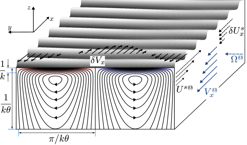
Figure 1: Sketch for Langmuir instability development. It was chosen $\theta=0.1\,\text{rad}$ and $\delta h/h^{\scriptscriptstyle(0)}=0.3$. In the $Oyz$-slice, the red and blue areas correspond to positive and negative $\delta\Omega_{x}$ respectively. Plane $y=0$ corresponds to the vertical middle plane of the depicted cell.

III Langmuir instability mechanism

In this Section we consider the Langmuir circulation instability problem. We assume that the unperturbed flow is a plane monochromatic wave propagating on the background of co-directed vertically sheared flow. Thus, the unperturbed flow is uniform in the spanwise direction, and the perturbation is modulated in the direction with some period, which is much larger that the wavelength. A sketch of the flow is depicted in Figure 1.

III.1 Unperturbed flow

We assume that the wave travels in the $x$ direction in Cartesian coordinate system. Thus, the wave potential

$$\phi^{{\scriptscriptstyle{(0)}}}=\real(\psi^{{\scriptscriptstyle{(0)}}}\exp[i\varphi^{{\scriptscriptstyle{(0)}}}+kz]\Big{)}$$ (23)

with $\psi^{{\scriptscriptstyle{(0)}}}$ and $k$ being potential amplitude and wave number respectively and the phase $\varphi^{{\scriptscriptstyle{(0)}}}=kx-\omega t$. The corresponding surface elevation rate is

$$\zeta^{{\scriptscriptstyle{(0)}}}=\real(h^{{\scriptscriptstyle{(0)}}}\exp[i\varphi^{{\scriptscriptstyle{(0)}}}]\Big{)}.$$ (24)

Without loss of generality we assume $h^{{\scriptscriptstyle{(0)}}}>0$. The slow current is shear flow aligned in the same $x$ direction

$$\bm{V}^{{\scriptscriptstyle{(0)}}}=\big{\{}V^{{\scriptscriptstyle{(0)}}}_{x},\,0,\,0\big{\}},\qquad\bm{\Omega}^{{\scriptscriptstyle{(0)}}}=\big{\{}0,\,\Omega^{{\scriptscriptstyle{(0)}}},\,0\big{\}},$$ (25)

where $\Omega^{{\scriptscriptstyle{(0)}}}(z)=\partial_{z}V^{{\scriptscriptstyle{(0)}}}_{x}(z)$. The relative slowness of the flow means that $\varepsilon\sim\Omega^{{\scriptscriptstyle{(0)}}}/\omega\ll 1$. One can think about the resulting motion as generalized Gouyon wave, see e.g. [22]. Here we apply our general scheme to find the influence of the shear onto the wave demonstrating the reproduction of the well-known result [17].

We start from the Stokes drift, which $x$ component is

$$U^{s{\scriptscriptstyle{(0)}}}_{x}=k\omega\big{(}h^{{\scriptscriptstyle{(0)}}}\big{)}^{2}e^{2kz}.$$ (26)

The vortex force (11) appears to be pure potential

$$\bm{f}^{V}=k\omega\Omega^{{\scriptscriptstyle{(0)}}}\big{(}h^{{\scriptscriptstyle{(0)}}}\big{)}^{2}e^{2kz}\big{\{}0,\,0,\,1\big{\}}$$ (27)

and, according to the equation (7), does not produce any contribution to the slow flow but only modifies the pressure.

Dispersion relation and, thus, phase velocity could be obtained from boundary conditions (17) and (19) on the free surface:

$$\big{(}-i\omega+ikV^{{\scriptscriptstyle{(0)}}}_{x}(0)\big{)}h^{{\scriptscriptstyle{(0)}}}=k\psi^{{\scriptscriptstyle{(0)}}},$$ (28)

$$\big{(}-i\omega+ikV^{{\scriptscriptstyle{(0)}}}_{x}(0)\big{)}\psi^{{\scriptscriptstyle{(0)}}}=-gh^{{\scriptscriptstyle{(0)}}}+p^{\varpi{\scriptscriptstyle{(0)}}},$$ (29)

with pressure (note that $\bm{u}^{\varpi\scriptscriptstyle(0)}=0$ for the geometry)

$$p^{\varpi{\scriptscriptstyle{(0)}}}=2ik\psi^{{\scriptscriptstyle{(0)}}}\Big{(}V^{{\scriptscriptstyle{(0)}}}_{x}(0)-2k\int\limits_{-\infty}^{0}dz\,e^{2kz}V^{{\scriptscriptstyle{(0)}}}_{x}(z)\Big{)}.$$ (30)

The solution of (28)-(29) with linear precision to $\Omega^{{\scriptscriptstyle{(0)}}}/\omega\ll 1$ term is

$$\omega=\sqrt{gk}+\omega^{\prime},\qquad\omega^{\prime}=2k^{2}\int\limits_{-\infty}^{0}dz\,e^{2kz}V^{{\scriptscriptstyle{(0)}}}_{x}(z),$$ (31)

and the phase velocity $\omega/k$ appears the same as in [17]. One can choose the reference system where $V_{x}^{\scriptscriptstyle(0)}|_{z=0}=0$. We assume that the shear flow is produced by surface stress co-directed with $Ox$-axis, as the Langmuir instability exists only in this case [23]. Then $\Omega^{\scriptscriptstyle(0)}>0$ if one considers the simplest case of constant sign shear and the correction to the wave frequency $\omega^{\prime}<0$. If we suppose the linear shear, ${V}^{{\scriptscriptstyle{(0)}}}_{x}=\Omega^{{\scriptscriptstyle{(0)}}}z$, then the correction to the wave frequency $\omega^{\prime}=-\Omega^{{\scriptscriptstyle{(0)}}}/2$.

III.2 Perturbation

It is assumed in CL2 mechanism [6] of Langmuir instability that an unstable mode includes a streamwise shear flow and a circulation in vertical-spanwise plane both modulated in the spanwise direction. Here we add into the mode structure the wave modulation, that can be thought as the result of scattering of initial wave on the modulated slow flow. We call the modulated wave oblique one after [24]. Hereinafter, we mark the contributions into the physical quantities describing the unstable mode with symbol ‘$\delta$’, so the full fields are now

$$\bm{V}=\bm{V}^{{\scriptscriptstyle{(0)}}}+\delta\bm{V},\quad \phi=\phi^{{\scriptscriptstyle{(0)}}}+\delta\phi,$$ (32)

$$\bm{\Omega}=\bm{\Omega}^{{\scriptscriptstyle{(0)}}}+\delta\bm{\Omega},\quad \zeta=\zeta^{{\scriptscriptstyle{(0)}}}+\delta\zeta.$$

The wave potential $\delta\phi$ and the surface elevation $\delta\zeta$ are:

$$\delta\phi = \real(\delta\psi\,e^{\lambda t}\exp[i\varphi^{\scriptscriptstyle(1)}+kz\big{]}\Big{)}$$ (33)

$$\delta\zeta = \real(\delta h\,e^{\lambda t}\exp[i\varphi^{\scriptscriptstyle(1)}\big{]}\Big{)},$$ (34)

where phase $\varphi^{\scriptscriptstyle(1)}=kx\cos\theta+ky\sin\theta-\omega t$ contains spanwise modulation with wave number $k\sin\theta$. The instability growth rate $\lambda$ is assumed to be much smaller compared to the wave frequency, $\lambda\ll\omega$, so the wave is assumed to be quasi-monochromatic. The correction to the oscillating part of the pressure could be represented in the same form (see Appendix A)

$$\delta{p}^{\varpi}=\real(\delta\tilde{p}^{\varpi}(z)\ e^{\lambda t}\exp[i\varphi^{\scriptscriptstyle(1)}\big{]}\Big{)}.$$ (35)

The dynamics and the spatial structure of the slow flow matches the dynamics of the interference between the initial and scattered waves averaged over the fast oscillations. Thus, the time dependence is exponential, $\exp(\lambda t)$, and the spatial structure of the slow flow is determined by the phase difference $\varphi^{\scriptscriptstyle(1)}-\varphi^{\scriptscriptstyle(0)}=ky\sin\theta+kx(\cos\theta-1)$:

$$\delta\bm{V}=\real(\delta\tilde{\bm{V}}(z)\,e^{\lambda t}\exp[i\big{(}\varphi^{\scriptscriptstyle(1)}-\varphi^{\scriptscriptstyle(0)}\big{)}\big{]}\Big{)}.$$ (36)

The same notations are considered for $\delta{\bm{\Omega}}$.

III.3 Getting equations

The next step is to derive the equations which define the dynamics of the perturbation in the approximation linear in its amplitude. The full system of equations to be linearized in the perturbation amplitude on the background of the flow described in Section III.1 consists of equations (16,17,19,21) for the fast oscillating motion and equations (13,14) for the slow flow. We note that one should keep only the first summand in the right-hand side of Eq. (20) since the amplitude of the perturbation is small. Note, that in the case we do not need to restore ${\bm{u}}^{\varpi}$ from ${\bm{\varpi}}^{u}$. The slow flow part of the perturbation is completely defined by $x$-components of velocity and vorticity $\delta\tilde{V}_{x}(z)$, $\delta\tilde{\Omega}_{x}(z)$ and its fast oscillating part is set by the oblique wave parameters $\delta\psi$, $\delta h$, so we establish equations for these quantities. We examine the problem in the limit $\theta\ll 1$, so we neglect all corrections which are relatively small as $\theta^{2}$. In particular, this means that $\cos\theta=1$ in our approximation and $x$-derivatives of slow flow variables are zero as the derivatives are proportional to $1-\cos\theta$. This approximation corresponds to $x$-independence of the slow flow perturbation adopted in [6] and allows one to introduce the stream function $\delta{\Psi}$ for the circulation in $Oyz$-plane:

$$\delta{V}_{y}=\partial_{z}\delta{\Psi},\quad\delta{V}_{\!z\,}=-\partial_{y}\delta{\Psi}=-ik\theta\delta{\Psi},$$

$$\delta{\Omega}_{x}=-(\partial_{z}^{2}-k^{2}\theta^{2})\delta{\Psi}.$$ (37)

Getting the final answer, we choose the particular case of linear shear flow, ${V}^{{\scriptscriptstyle{(0)}}}_{x}=\Omega^{{\scriptscriptstyle{(0)}}}z$, consider the limit of small Langmuir number $\mathrm{La}\ll\theta^{2}$, see (59), and neglect the corrections which are relatively small as $\theta$ as well. It is convenient to divide the solution into two steps. The first step is determining the slow current part via the oblique wave parameters. The step can be implemented analytically in the case of linear unperturbed shear ${V}^{{\scriptscriptstyle{(0)}}}_{x}=\Omega^{{\scriptscriptstyle{(0)}}}z$. On the second step, we define the instability growth rate $\lambda$ from the requirement that free surface equations (17) and (19) have nontrivial solution. We also adopt below that all quantities describing the unstable mode are complex, that is, in particular, one should drop $\mathrm{Re}$ in definitions (33,34,35,36) for the perturbation and (23,24) for the initial wave.

Let us first linearize in the perturbation amplitude equation (13) and equation (8) written for the slow flow:

$$\big{(}\lambda-\nu_{\scriptscriptstyle T}\Delta+V^{{\scriptscriptstyle{(0)}}}_{x}\partial_{x}\big{)}\delta\bm{V}+\delta{V}_{\!z\,}\bm{\Omega}^{{\scriptscriptstyle{(0)}}}+\operatorname{grad}\delta\overline{P}=\delta\bm{f}^{\scriptscriptstyle V},$$ (38)

$$\big{(}\lambda-\nu_{\scriptscriptstyle T}\Delta+V^{{\scriptscriptstyle{(0)}}}_{x}\partial_{x}\big{)}\delta\bm{\Omega}-\Omega^{\scriptscriptstyle(0)}\big{[}\delta\Omega_{z}\bm{e}^{x}+\partial_{y}\delta\bm{V}\big{]}=$$

$$=\operatorname{curl}\delta\bm{f}^{\scriptscriptstyle V},$$ (39)

where we took into consideration the variation of vortex force

$$\delta\bm{f}^{\scriptscriptstyle V}=\big{[}\bm{U}^{s{\scriptscriptstyle{(0)}}},\,\delta\bm{\Omega}\big{]}+\big{[}\delta\bm{U}^{s},\,\bm{\Omega}^{{\scriptscriptstyle{(0)}}}\big{]}$$ (40)

as well. The correction to the Stokes drift velocity defined in (12) is

$$\delta\bm{U}^{s}=\frac{1}{2}\,\partial_{l}\big{(}\delta s_{l}^{*}\bm{u}^{\phi{\scriptscriptstyle{(0)}}}\big{)}+\frac{1}{2}\,\partial_{l}\big{(}s^{{\scriptscriptstyle{(0)}}*}_{l}\delta\bm{u}^{\phi}\big{)},$$ (41)

where symbol ^⋆ denotes complex conjugation. In the limit of small angle $\theta$, the Stokes drift perturbation is

$$\delta U^{s}_{x}={} 2ik^{2}h^{{\scriptscriptstyle{(0)}}}\delta\psi\,e^{\lambda t+2kz}\exp[i(\varphi^{\scriptscriptstyle(1)}-\varphi^{{\scriptscriptstyle{(0)}}}))\big{]},$$ (42)

and $\delta U^{s}_{y}=\theta\,\delta U^{s}_{x}$, but $y$-component is not interesting because it does not produce any contribution into vortex force (40). The perturbation (40) of the vortex force appears to be directed in $yz$-plane. Now we take $x$-components in equations (38,III.3) and obtain in our approximations

$$\big{[}\lambda-\nu_{\scriptscriptstyle T}\big{(}\partial_{z}^{2}-k^{2}\theta^{2}\big{)}\big{]}\delta\tilde{V}_{x}+\Omega^{{\scriptscriptstyle{(0)}}}\delta\tilde{V}_{z}=0.$$ (43)

$$\big{[}\lambda-\nu_{\scriptscriptstyle T}\big{(}\partial_{z}^{2}-k^{2}\theta^{2}\big{)}\big{]}\delta\tilde{\Omega}_{x}+2ik^{2}\theta U^{s{\scriptscriptstyle{(0)}}}\delta\tilde{V}_{x}=$$

$$=ik\theta\Omega^{\scriptscriptstyle(0)}\delta\tilde{U}^{s}_{x}.$$ (44)

Note that $x$-component of square bracket in (III.3) was neglected as it is equal to $\partial_{x}\delta V_{y}$. Equations should be supplemented with boundary conditions on the free surface (14)

$$\partial_{z}\delta V_{x}\big{|}_{z=0}=\partial_{z}\delta V_{y}\big{|}_{z=0}=0,\quad\delta{V}_{\!z\,}\big{|}_{z=0}=0.$$ (45)

Next we rewrite equations (17,19),

$$(\lambda-i\omega)\delta{h}={} k\delta\psi+h^{\scriptscriptstyle(0)}\partial_{z}\delta{V}_{\!z\,}\big{|}_{z=0},$$ (46)

$$(\lambda-i\omega)\delta\psi={} -g\delta{h}+\delta{p}^{\varpi}\big{|}_{z=0}.$$ (47)

Taking into account the boundary conditions for the slow current (45), the pressure $\delta\tilde{p}^{\varpi}$ taken at the surface can be presented in the form (see (67))

$$\delta\tilde{p}^{\varpi}\big{|}_{z=0} = -\psi^{\scriptscriptstyle(0)}\int\limits_{-\infty}^{0}dz\,e^{2kz}(\partial_{z}^{2}-k^{2}\theta^{2})\big{(}i\delta\tilde{V}_{x}+\delta\tilde{V}_{z}\big{)}+$$ (48)

$$+i\Omega^{\scriptscriptstyle(0)}\big{|}_{z=0}\delta{\psi}.$$

III.4 Solution

Now we assume, that the perturbations growth rate $\lambda$ is large compared to viscous decay rate of the slow flow component of the perturbation. Since the Stokes drift in (43) penetrates on depth $\sim 1/k$, the vertical scale of $\delta\Omega_{x}$ is the same. This means, that the viscous damping rate is

$$\nu_{\scriptscriptstyle T}k^{2}\ll\lambda.$$ (49)

Below we show that the inequality is equivalent to the limit of small Langmuir number. In the limit, the viscous scale $\delta_{\nu}\sim\sqrt{\nu_{\scriptscriptstyle T}/\lambda}$ for the slow flow is less than the wave penetration depth $1/k$, $k\delta_{\nu}\ll 1$ and $\lambda$ prevails the viscous terms in square brackets in (43,III.3). We neglect the viscous term in equation (43) and obtain

$$\delta\tilde{V}_{x}=-\frac{\Omega^{{\scriptscriptstyle{(0)}}}}{\lambda}\delta\tilde{V}_{z}=\frac{ik\theta\Omega^{{\scriptscriptstyle{(0)}}}}{\lambda}\delta\tilde{\Psi}$$ (50)

due to definition (III.3). According to (50), the mutual signs of $\delta\tilde{V}_{x}$ and $\delta\tilde{V}_{z}$ are fixed due to implied $\Omega^{{\scriptscriptstyle{(0)}}}>0$ and, as it will be shown below, the increment is real, $\lambda>0$. Downward flow in the circulation corresponds to maximum in the amplitude of the shear flow. On the other hand, the downward flow corresponds to divergent stream lines on the surface, i.e. areas where a surface contamination is collected along $x$-oriented lines. Under the same approximation, equation (III.3) gives

$$(k^{-2}\partial_{z}^{2}-\theta^{2})\delta\tilde{\Psi}+\mu^{2}\,e^{2kz}\delta\tilde{\Psi}=\sqrt{\varepsilon}\,\mu\,e^{2kz}\delta{\psi},$$ (51)

where the dimensionless quantities $\mu$ and $\varepsilon$ are

$$\mu=\dfrac{\sqrt{2\Omega^{\scriptscriptstyle{(0)}}\omega}}{\lambda}\,kh^{\scriptscriptstyle{(0)}}\theta,\quad\varepsilon=\dfrac{2\Omega^{\scriptscriptstyle{(0)}}}{\omega^{\,}}\ll 1.$$ (52)

As we are considering inviscid problem, the boundary conditions for the stream function are

$$\delta\tilde{\Psi}(0)=\delta\tilde{\Psi}(-\infty)=0$$ (53)

instead of (45). Note that we gain the CL2-model equation [6] if we neglect the variation of Stokes drift, i.e. let the right-hand side of (51) being equal to zero.

Further we consider linear shear flow, so parameters $\mu$ and $\varepsilon$ are $z$-independent after $\Omega^{\scriptscriptstyle{(0)}}$. In the absence of Stokes drift variation in (51), the eigenvalue problem (51,53) leads to the solution $\delta\tilde{\Psi}={\mathrm{J}}_{\theta}(\mu\,e^{kz})$ and boundary condition ${\mathrm{J}}_{\theta}(\mu)=0$ [6], where $\mathrm{J}_{n}(\mu)$ is Bessel function of $n$-th order. Thus the perturbation grows rate in CL2-model corresponds to the lowest root $\mu_{\text{\tiny{CL2}}}\approx 2.4$ in the limit $\theta\ll 1$. Now we restore the right-hand side of (53). The equation (51) can be solved analytically for the constant initial shear flow:

$$\delta\tilde{\Psi}=\dfrac{\sqrt{\varepsilon}}{\mu}\Bigg{[}1-\Big{(}1+\dfrac{1-{\mathrm{J}}_{0}(\mu)}{{\mathrm{J}}_{0}(\mu)}\,e^{|\theta|kz}\Big{)}{\mathrm{J}}_{0}\big{(}\mu\,e^{kz}\big{)}\Bigg{]}\delta{\psi}.$$ (54)

Expression (54) is not exact, there are corrections for the exact solution which are relatively small as $\theta$. With the accuracy, one should put the exponent $e^{|\theta|kz}\to 1$ when $kz\sim 1$ so the square bracket in (54) is equal to $1-{\mathrm{J}}_{0}\big{(}\mu\,e^{kz}\big{)}/{\mathrm{J}}_{0}(\mu)$. At large depths $z\gtrsim 1/k\theta$, the stream function decays exponentially as the square bracket in (54) is $(1-1/{\mathrm{J}}_{0}(\mu))\,e^{|\theta|kz}$. Thus, the circulation penetrates $1/k\theta$ deep. However, the vorticity related to the stream function according to (III.3) penetrates only $1/k$ deep,

$$\delta\tilde{\Omega}_{x}=i\sqrt{\varepsilon}\,\dfrac{\mu{\mathrm{J}}_{0}(\mu\,e^{kz})}{{\mathrm{J}}_{0}(\mu)}\,e^{2kz}\omega k\delta{h},$$ (55)

where we used approximate equality $\delta\psi=-i(\omega/k)\delta h$. Note that in CL2 model, the vorticity has the same vertical dependence in our approximations, $\delta\tilde{\Omega}_{x}=(\mu k)^{2}e^{2kz}{\mathrm{J}}_{0}(\mu e^{kz})$.

Equations (50,54) express the slow flow via the oblique wave parameters $\delta h$, $\delta\psi$. To be able to write explicitly equations (46,46) in terms of the parameters, we need to do this first for the residual part of pressure $\delta{p}^{\varpi}$ using (48):

$$\delta\tilde{p}^{\varpi}\big{|}_{z=0}=\big{(}(F(\mu)+1)\lambda+iF(\mu)\Omega^{{\scriptscriptstyle{(0)}}}\big{)}\delta{\psi},$$ (56)

where a function

$$F(\mu)=1+\Big{(}\mu-\dfrac{1}{\mu}\Big{)}\dfrac{{\mathrm{J}}_{1}(\mu)}{{\mathrm{J}}_{0}(\mu)}$$ (57)

is even in $\mu$. It follows from (55) also, that $\partial_{z}\delta\tilde{V}_{z}|_{z=0}=-i\sqrt{\varepsilon}({\mathrm{J}}_{1}(\mu)/{\mathrm{J}}_{0}(\mu))k^{2}\theta\,\delta\psi$ in (46). The linear system of equations (46,47) for $\delta h$, $\delta\psi$ has a nontrivial solution if $F(\mu)=0$ in the first precision with respect to small parameters $\varepsilon$ and $\theta$. Among all existing solutions we should choose that corresponding to positive and minimal real part of $\lambda$. The numerical solution is

$$\mu_{\star}\simeq 1.67,\quad\lambda=\dfrac{\sqrt{2\Omega^{\scriptscriptstyle{(0)}}\omega}}{\mu_{\star}}\,kh^{\scriptscriptstyle{(0)}}|\theta|.$$ (58)

As $\mu_{\star}<\mu_{\scriptscriptstyle CL2}$, obtained growth increment $\lambda$ (58) is greater than that found in [6]. Hence, the unstable mode does contain the oblique wave component. Knowing that $\mu\sim 1$, let us rewrite the inequality (49). We introduce friction velocity $u_{\ast}$ according to definition $\Omega^{\scriptscriptstyle{(0)}}=u_{\ast}^{2}/\nu_{\scriptscriptstyle T}$. Then (49) means that Langmuir number

$$\mathrm{La}\equiv\frac{\nu_{\scriptscriptstyle T}^{3}k^{2}}{\omega(h^{\scriptscriptstyle(0)})^{2}u_{\ast}^{2}}\ll\theta^{2}.$$ (59)

Let us also test the properties of the solution with respect to changing the sign of angle $\theta$, that leads to $\mu\to-\mu$ as well. Without loss of generality we can adopt that $\delta h$ is pure real, $\delta h<0$, and the phase difference between the initial and oblique waves along streamwise direction is small, $k\theta^{2}x\ll 1$, so phase difference $\varphi^{\scriptscriptstyle(1)}-\varphi^{\scriptscriptstyle(0)}=k\theta y$ in (36). Then both $\delta\tilde{V}_{z}$ (III.3) and $\delta\tilde{V}_{x}$ (50) are pure real and even in $\theta$, so $\delta V_{z}\propto\cos(k\theta y)$ (including the sign) is even function of $\theta$ after $\delta\tilde{V}_{x}$, whereas $\delta\tilde{V}_{y}$ is pure imaginary and odd in $\theta$, so $\delta V_{y}\propto-\theta\sin(k\theta y)$ (the sign is taken at the surface) is even function of $\theta$ as well. This means that the unstable mode is twice degenerate; two possible configurations have identical slow flow spatial structure and oblique waves with opposite spanwise wave numbers. The derived spatial distribution is schematically plotted in Figure 1.

IV Discussion

Presented analysis of Langmuir instability assumes that the flow has exactly periodic structure in space. In reality, the periodicity should be lost at some length $L_{c}$. For the analysis to be valid, the length should be greater than the distance which wave passes during the characteristic time $1/\lambda$ along streamwise direction, that is $L_{c,x}>\omega/(k\lambda)$. Taking into account (58,52), one can rewrite the inequality in the form $L_{c,x}>1/(\sqrt{\varepsilon}\,\theta\,kh^{\scriptscriptstyle(0)}k)$, that much exceeds the period in spanwise direction. In spanwise direction, the periodicity should be kept at smaller length $L_{c,y}\sim\theta L_{c,x}$. If the periodicity appears to be disrupted at shorter distances, then the oblique wave is not correlated with the Langmuir circulation and one should drop it out during the Langmuir instability analysis. As a result, one arrives back to CL2-model [6], where only $x$-independence of the flow at distances greater than $1/(k\theta)$ is assumed.

Considering an extension of the scope of our approach, we believe, that the developed mathematical scheme should be appropriate for the analysis of wave-current interaction in flow confined in a basin, see e.g. [25, 26]. The confinement preserves correlation between vortical flow and surface waves, which are mostly standing ones in the case. At initial stage, when only surface waves are excited, the leading mechanism of the interaction is virtual wave stress [20, 26], which can be enhanced due to presence of surface contamination in a form of liquid elastic film [27]. However, during the development of large-scale vortical flow, oblique waves appears that is evidence of the wave scattering by the vortical flow [25]. The presented approach, combined with a more detailed analysis of experimental data, can answer whether a wave-current interaction loop plays any role in formation of large-scale flow, along with other mechanisms, including the two-dimensional inverse energy cascade [28].

V Acknowledgments

The work was supported by Russian Science Foundation (project no. 23-72-30006).

Appendix A Contribution into pressure related to high-frequency part of the vorticity

The equation on oscillating part of pressure follows from Navier-Stokes equation for wave motion

$$\partial_{t}\bm{u}^{\phi}+\left(\bm{u}^{\phi}\nabla\right)\bm{V}+\left(\bm{V}\nabla\right)\bm{u}^{\phi}+\partial_{t}\bm{u}^{\varpi}+\left(\bm{u}^{\varpi}\nabla\right)\bm{V}+\left(\bm{V}\nabla\right)\bm{u}^{\varpi}=-\nabla p^{u}+\bm{g}$$ (60)

Let us group potential and vortical terms

$$\Bigl{(}\partial_{t}\bm{u}^{\varpi}+\left(\bm{u}^{\varpi}\nabla\right)\bm{V}+\left(\bm{V}\nabla\right)\bm{u}^{\varpi}\Bigr{)}-\left[\bm{u}^{\phi}\bm{\Omega}\right]=-\nabla\Bigl{(}p^{u}+gz+\left(\partial_{t}+V_{i}\partial_{i}\right)\phi\Bigr{)},$$ (61)

using

$$\left(\bm{u}\nabla\right)\bm{V}+\left(\bm{V}\nabla\right)\bm{u}=\nabla\left(\bm{u}\bm{V}\right)-\left[\bm{V}\bm{\omega}\right]-\left[\bm{u}\bm{\Omega}\right],$$

valid for incompressible vector fields. The gradient term in right-hand side of (61) we interpret as vortical part of pressure which we denote as $p^{\varpi}$,

$$p^{\varpi}\equiv p^{u}+gz+\left(\partial_{t}+V_{i}\partial_{i}\right)\phi$$ (62)

$$\Delta p^{\varpi}=f^{\varpi},\qquad f^{\varpi}=\partial_{i}\phi\,\Delta V_{i}+2\partial_{j}u^{\varpi}_{i}\,\partial_{i}V_{j}.$$ (63)

The boundary condition for $p^{\varpi}$ on the free surface is following from $z$-component of equation (61). Taking into account the smallness of spatial derivatives of $\bm{V}$, we present

$$\left.\partial_{z}p^{\varpi}\right|_{z=0}=\partial_{\alpha}\phi\,\partial_{z}V_{\alpha},\qquad\left.p^{\varpi}\right|_{z\rightarrow-\infty}\rightarrow 0.$$ (64)

The differential problem (63), (64) could be solved analytically in Fourier space (${\bf q}$ denotes Fourier harmonic in $Oxy$-здате)

$$\left(\partial^{2}_{z}-q^{2}\right)\delta{p}^{\varpi}_{\bf q}=f^{\varpi}_{\bf q},\qquad\delta{p}^{\varpi}_{\bf q}=-\dfrac{e^{qz}}{2q}\int\limits_{-\infty}^{0}dz^{\prime}e^{qz^{\prime}}f^{\varpi}_{\bf q}(z^{\prime})-\int\limits_{-\infty}^{0}dz^{\prime}\dfrac{e^{-q|z-z^{\prime}|}}{2q}f^{\varpi}_{\bf q}(z^{\prime})+\frac{e^{qz}}{q}\big{(}\partial_{\alpha}\phi\partial_{z}V_{\alpha}\big{)}_{\bf q}.$$ (65)

Now we turn to calculations in the sake of Langmuir instability analysis. Using the estimation (22) we get $f^{\varpi}=\partial_{i}\phi\,\Delta V_{i}$ in (63). Thus,

$$\delta{p}^{\varpi}_{\bf q}\big{|}_{z=0}=-\dfrac{1}{q}\int\limits_{-\infty}^{0}dz\,e^{qz}\big{(}\partial_{i}\phi\Delta V_{i}\big{)}_{\bf q}+\dfrac{1}{q}\partial_{\alpha}\big{(}\phi\partial_{z}V_{\alpha}\big{)}_{\bf q}.$$ (66)

Using this expression, let us prove the equality (35). We substitute (33) and (36) in (66) and by direct calculations we show that only harmonics oscillating as $\exp[ikx\cos\theta+iky\sin\theta]$ appears nonzero (note that we should set ${\bf q}=k\{\cos\theta,\sin\theta\}$). According to definition (35) we obtain

$$\delta\tilde{p}^{\varpi}\big{|}_{z=0}=-\psi^{{\scriptscriptstyle{(0)}}}\int\limits_{-\infty}^{0}dz\,e^{2kz}\big{(}\partial_{z}^{2}-k^{2}\sin^{2}\theta\big{)}\big{(}i\delta\tilde{V}_{x}+\delta\tilde{V}_{z}\big{)}+i\delta\psi\Omega^{\scriptscriptstyle{(0)}}\big{|}_{z=0}\cos\theta+\psi^{{\scriptscriptstyle{(0)}}}(\partial_{x}+ik)\partial_{z}\delta\tilde{V}_{x}\Big{|}_{z=0}$$

$$+ik\psi^{{\scriptscriptstyle{(0)}}}\sin\theta\partial_{z}\delta\tilde{V}_{y}\Big{|}_{z=0}.$$ (67)

References

- Hamlington et al. [2014] P. E. Hamlington, L. P Van Roekel, B. Fox-Kemper, K. Julien, and G. P. Chini. Langmuir–submesoscale interactions: Descriptive analysis of multiscale frontal spindown simulations. Journal of Physical Oceanography, 44(9):2249–2272, 2014.
- Thorpe [2004] S.A. Thorpe. Langmuir circulation. Annu. Rev. Fluid Mech., 36:55–79, 2004.
- Teixeira [2019] Miguel A.C. Teixeira. Langmuir circulation and instability. In J. Kirk Cochran, Henry J. Bokuniewicz, and Patricia L. Yager, editors, Encyclopedia of Ocean Sciences (Third Edition), pages 92–106. Academic Press, Oxford, 2019.
- Weller and Price [1988] R. A. Weller and J. F. Price. Langmuir circulation within the oceanic mixed layer. Deep Sea Research Part A. Oceanographic Research Papers, 35(5):711–747, 1988.
- Chang et al. [2019] H. Chang, H. S. Huntley, A.D. Kirwan, D. F. Carlson, J. A. Mensa, S. M., G. Novelli, T. M. Özgökmen, B. Fox-Kemper, B. Pearson, et al. Small-scale dispersion in the presence of langmuir circulation. Journal of physical oceanography, 49(12):3069–3085, 2019.
- Craik [1977] A. D. D. Craik. The generation of langmuir circulations by an instability mechanism. Journal of Fluid Mechanics, 81(2):209–223, 1977.
- Leibovich [2009] S. Leibovich. Langmuir circulation and instability. Elements of Physical Oceanography: A derivative of the Encyclopedia of Ocean Sciences, 124(2):288, 2009.
- Faller and Caponi [1978] A. J. Faller and E. A. Caponi. Laboratory studies of wind-driven langmuir circulations. Journal of Geophysical Research: Oceans, 83(C7):3617–3633, 1978.
- Sullivan and McWilliams [2019] P. P. Sullivan and J. C. McWilliams. Langmuir turbulence and filament frontogenesis in the oceanic surface boundary layer. Journal of Fluid Mechanics, 879:512–553, 2019.
- Craik and Leibovich [1976] A. D. D. Craik and S. Leibovich. A rational model for langmuir circulations. Journal of Fluid Mechanics, 73(3):401–426, 1976.
- Craik [1982] A. D. D. Craik. Wave-induced longitudinal-vortex instability in shear flows. Journal of Fluid Mechanics, 125:37–52, 1982.
- Kawamura [2000] T. Kawamura. Numerical investigation of turbulence near a sheared air–water interface. part 2: Interaction of turbulent shear flow with surface waves. Journal of marine science and technology, 5:161–175, 2000.
- Veron and Melville [2001] F. Veron and W. K. Melville. Experiments on the stability and transition of wind-driven water surfaces. Journal of Fluid Mechanics, 446:25–65, 2001.
- Fujiwara and Yoshikawa [2020] Y. Fujiwara and Y. Yoshikawa. Mutual interaction between surface waves and langmuir circulations observed in wave-resolving numerical simulations. Journal of Physical Oceanography, 50(8):2323–2339, 2020.
- Leibovich [1977] S. Leibovich. On the evolution of the system of wind drift currents and langmuir circulations in the ocean. part 1. theory and averaged current. Journal of Fluid Mechanics, 79(4):715–743, 1977.
- Lamb [1932] H. Lamb. Hydrodynamics. University Press, 1932.
- Stewart and Joy [1974] R. H. Stewart and J. W. Joy. Hf radio measurements of surface currents. In Deep sea research and oceanographic abstracts, volume 21, pages 1039–1049. Elsevier, 1974.
- Longuet-Higgins [1953] M. S. Longuet-Higgins. Mass transport in water waves. Mathematical and Physical Sciences, 245(903):535–581, 1953.
- Nicolás and Vega [2003] J. A. Nicolás and J. M. Vega. Three-dimensional streaming flows driven by oscillatory boundary layers. Fluid Dynamics Research, 32(4):119–139, 2003.
- Filatov et al. [2016] S. V. Filatov, V. M. Parfenyev, S. S. Vergeles, M. Yu. Brazhnikov, A. A. Levchenko, and V. V. Lebedev. Nonlinear generation of vorticity by surface waves. Physical Review Letters, 116(5):054501, 2016.
- Garrett [1976] C. Garrett. Generation of langmuir circulations by surface waves — a feedback mechanism. Journal of Marine Research, 34:117, 1976.
- Abrashkin et al. [2022] A. A. Abrashkin, E. N. Pelinovsky, et al. Gerstner waves and their generalizations in hydrodynamics and geophysics. Phys. Usp., 65:453–467, 2022.
- Leibovich [1983] S. Leibovich. The form and dynamics of langmuir circulations. Annual Review of Fluid Mechanics, 15(1):391–427, 1983.
- Craik [1970] A. D. D. Craik. A wave-interaction model for the generation of windrows. Journal of Fluid Mechanics, 41(4):801–821, 1970.
- Filatov et al. [2018] S. V. Filatov, A. V. Orlov, M. Yu. Brazhnikov, and A. A. Levchenko. Experimental simulation of the generation of a vortex flow on a water surface by a wave cascade. JETP Letters, 108:519–526, 2018.
- Filatov et al. [2022] S.V. Filatov, A.V. Poplevin, A.A. Levchenko, and V.M. Parfenyev. Generation of stripe-like vortex flow by noncollinear waves on the water surface. Physica D: Nonlinear Phenomena, 434:133218, 2022.
- Parfenyev et al. [2019] V.M. Parfenyev, S.V. Filatov, M. Yu. Brazhnikov, S.S. Vergeles, and A.A. Levchenko. Formation and decay of eddy currents generated by crossed surface waves. Physical Review Fluids, 4(11):114701, 2019.
- Colombi et al. [2022] R. Colombi, N. Rohde, M. Schlüter, and A. von Kameke. Coexistence of inverse and direct energy cascades in faraday waves. Fluids, 7(5):148, 2022.