Non-reversible Monte Carlo: an example of “true” self-repelling motion

Abstract

We link the large-scale dynamics of non-reversible Monte Carlo algorithms as well as a lifted TASEP to an exactly soluble model of self-repelling motion. We present arguments for the connection between the problems and perform simulations, where we show that the empirical distribution functions generated from Monte Carlo are well described by the analytic solution of self-repelling motion.

Introduction

Non-reversible Monte Carlo sampling as developed for hard disks [1], and its generalisation to arbitrary potentials [2, 3, 4] has many wonderful properties which facilitate the equilibration of large complex systems faster than conventional Monte Carlo, or molecular dynamics algorithms. However, analytic understanding of the large-scale, effective dynamics is lacking. This is in strong contrast to, for instance, molecular dynamics which generate the Navier-Stokes equations at large scales. Extensive theoretical analysis of the mode structure of these hydrodynamic equations gives us the slow hydrodynamic modes of sound, vorticity and heat propagation, which limit the large-scale sampling of a fluid.

What are the equivalent statements for event chain Monte Carlo? What are the slow, hydrodynamic modes? This paper aims to present the continuum, coarse-grained equations describing event-chain simulation and demonstrate their equivalence to an exactly soluble model of a growing polymer. Clearly, if one understands the temporal evolution of the coarse-grained equations, it will be possible to make exact statements on the evolution of densities and correlations, and perhaps find better implementations in the future. The present paper makes a direct link with “true” self-repelling motion, [5] which has been much studied using a variety of physical methods including scaling [6, 7] and renormalisation [8]. Recently this model has been studied using advanced methods based on interacting Brownian paths, which have led to exact, analytic results for the dynamical properties [9, 10, 11].

In this paper, we introduce the self-avoiding model, together with the exact results for its time evolution. We then summarise the behaviour of a class of non-reversible algorithms before arguing analytically that there is a link between these two dynamical systems. Finally, we present numerical evidence as to the identity of distribution functions with data coming from event chain simulation of harmonic chains, as well as simulation of a lifted TASEP (Totally Asymmetric Simple Exclusion Process).

True self-avoiding motion

The model for the “true” self-avoiding walk was introduced, [5] as a dynamic model of polymer growth, in contrast to an equilibrated statistical ensemble of equilibrated polymers. On a lattice, monomers are added successively to a chain, trying to avoid places where the polymer has already passed. The probability of of choosing a site $i$, which has been visited $L_{i}(t)$ times is then

$$p_{i}(t+1)=\frac{e^{-\lambda L_{i}(t)}}{\sum_{j}e^{-\lambda L_{j}(t)}}$$ (1)

Where the sum is over all neighbours $j$ of the current position at time $t$. The model has infinite memory, required to calculate the placement probabilities of the new monomer.

It was argued, [5] that this dynamic process has a continuum limit so that the effective, large-scale behaviour is of the form

$$\frac{d{\textbf{X}(t)}}{dt} = -\nabla L(t,{\textbf{X}}(t))+\xi(t)$$ (2)

$$\frac{dL(t,{\textbf{x}})}{dt} = \,\,\delta({\textbf{x}}-{\textbf{X}(t)})$$ (3)

The function, $L(t,{\textbf{x}})$, a local time, cumulates memory as to the occupation of the position ${\textbf{X}}(t)$. The motion of the end of the growing polymer is then repelled by regions where $L(t,{\textbf{x}})$ has become large, in a manner which is analogous to the original lattice model. This continuum model is then amenable to many of the formal methods of field theory [8].

Distributions functions of the model

Remarkably, the equations (2, 3) in one dimension lead to an explicitly solvable model [10, 11] involving time scaling in $t^{2/3}$ or $t^{1/3}$ for distribution functions; the Langevin-like eq. (2), does not lead to Brownian scaling in $t^{1/2}$. The exact solutions displayed in [11] show that two important distributions of physical variables exhibit scaling forms:

$$\rho_{1}(t,x) = t^{-2/3}\nu_{1}(xt^{-2/3})$$ (4)

$$\rho_{2}(t,h) = t^{-1/3}\nu_{2}(ht^{-1/3})$$ (5)

$\rho_{1}(t,x)$ is the distribution of displacement of the process after time $t$; in the original polymer problem of [5] it is the distribution of end-to-end separations. $\rho_{2}(t,h)$ is the distribution of $h(t)=L(t,X(t))$, the number of previous visits to the endpoint of the polymer. The scaling functions are explicitly given by

$$\nu_{1}(x) = \sum_{k=1}^{\infty}\frac{p_{k}}{2}\delta^{\prime}_{k}f_{2/3}(\delta^{\prime}_{k}|x|)$$ (6)

$$\nu_{2}(h) = \frac{2\cdot 6^{1/3}\sqrt{\pi}}{\Gamma{(1/3)}^{2}}e^{-(8h^{3})/9}U(1/6,2/3,(8h^{3})/9)$$ (7)

$f_{2/3}(x)$ is the Mittag-Leffler function. $\delta^{\prime}_{k}$ and $p_{k}$ are calculated from the k’th zero of the derivative of an Airy function [11], $U$ is a confluent hypergeometric function of the second kind [12].

Scaling argument for motion

A scaling argument [7], allows one to find the exponents describing the solutions. Let motion occur on the length scale $t^{\alpha}$ in time $t$. Then $L$ must be of the form

$$L(t,x)\sim t^{(1-\alpha)}g(x/t^{\alpha})$$ (8)

The driving force from eq. (2), $-\nabla L(t,x)$, then scales as $t^{(1-2\alpha)}g^{\prime}(x/t^{\alpha})$. If this force acts over the time $t$, it generates motion $\sim t^{(2-2\alpha)}$. It is natural that this motion is comparable to the total extent of the motion, $t^{\alpha}$, so $t^{(2-2\alpha)}$ = $t^{\alpha}$, and $\alpha=2/3$.

Event Chain Monte Carlo

Event chain Monte Carlo methods are lifted variants of reversible Monte Carlo, where a single “active” particle is mobile, and at (to be determined) event times transfers motion to another particle, thereby avoiding the rejection step of reversible Monte Carlo methods [13]. We here consider event chain algorithms suitable for simulation of models with continuous potentials [2, 4].

The total energy function is broken into a sum of “factor potentials”. Each of these factors is then able to veto the motion of the active particle when a stochastic criterion, is violated. At the moment of veto, motion then transfers to another member of the factor which emitted the veto. In the case of the sampling of a chain, each particle is in direct interaction with its two neighbours, the factor potentials are then just the contribution of each bond to the total energy.

Particularly exciting results with this algorithm were found for low-dimensional XY spins [14] where it was argued that in one dimension the dynamics are characterized by a dynamic exponent, $z=1/2$. This exponent links the relaxation time $\tau$ (in sweeps) of a system $N$ spins via $\tau\sim N^{z}$. This result is smaller (hence, better) than is found in conventional reversible Monte Carlo or molecular dynamics where one finds $z=2$ or $z=1$. This exceptional scaling was generalized to more general models, including hard spheres and Lennard-Jones chains where a detailed study of the dynamics was performed [15]. As noted in [15], a dynamic exponent of $z=1/2$, requires that the motion is indeed characterised by hyperdiffusion, $x\sim t^{2/3}$. Rather remarkably, independent of the underlying physical system the large-scale dynamic processes obey identical hyper-diffusive dynamics. We also note that scaling of the form eq. (5) was found for the local time (see in particular [15] Fig. 9).

Very similar phenomenology has recently been demonstrated in a lattice model, a lifted version of the widely studied simple exclusion process [16, 17]. Here too, strong numerical evidence, constructed via the Bethe ansatz, points to a non-trivial scaling of solutions involving $t^{2/3}$. We conclude that this unusual scaling in time is observed in a wide variety of physical models (with very different underlying interactions) undergoing non-reversible dynamics subject to balance, without detailed balance.

Argument for algorithmic optimality

We note that motion $x\sim t^{2/3}$ is optimal for sampling via of a single tracer particle (we do not consider algorithms involving global updates) leading to complete resampling of the modes of a one-dimensional system: Consider a section of $l$ elements within a system of particles. Peierls argument, [18], tells us that the fluctuations in this section increase as $|\Delta l|\sim l^{1/2}$. Consider now the algorithm that has been run for $t$ steps to sample this system, with $x\sim t^{\alpha}$. Thus, length fluctuations, if the section is fully re-equilibrated, are $|\Delta l|\sim t^{\alpha/2}$. From eq. (8) we see that the number of visits to the starting point of the simulation is $L(t,0)\sim t^{1-\alpha}$. If we identify the two expressions for the displacement then $t^{1-\alpha}\sim|\Delta l|\sim t^{\alpha/2}$, or $\alpha=2/3$. Thus the amplitude of fluctuations, needed to re-equilibrate the section, is comparable to the number of returns of the algorithm to the origin, and thus the maximum displacement that can be generated for the origin in the time $t$.

Self-repelling motion and non-reversible simulation

Consider simulating an elastic chain at temperature, $T=1$, with harmonic springs of unit strength, starting with a zero-temperature configuration. For concreteness, we take the active particle to move in the $+x$ direction. The event chain algorithm proposes, at each time step, a displacement of the active particle which is vetoed after motion by a distance $O(1)$. Let us consider now a section of the chain, of $l+1$ sites of the system $[0,l]$, which has been uniformly stretched, after running the algorithm for some time. For this to have occurred, there must have been more visits to the site labelled $l$ than to the site $0$, for instance for l=4 the zig-zag trajectory $(01234)(32)(1234)(3)(234)(34)$ generates a stretched chain with number of visits for each site, $L_{i}=[1,2,4,6,\dots]$. This stretching then influences the future motion of the active particle. Such a stretch leads to a higher veto rate for transfers of the activity to the left of the chain, opposite to the gradient in $L_{i}$. However, this is exactly the phenomenology of eq. (2). If the exact details of the local update rule are not crucial in the dynamics and some form of large-scale universality applies eqs. (2, 3) are clearly candidates for a coarse-grained description of the motion generated by event chain Monte Carlo. In event chain simulation in higher dimension, we understand that relative motion of particles leads to a heterogeneous buildup in stress which will then back-react on the motion of the active particle, leading to a very similar coupling of motion and history.

Numerical results

Elastic chain

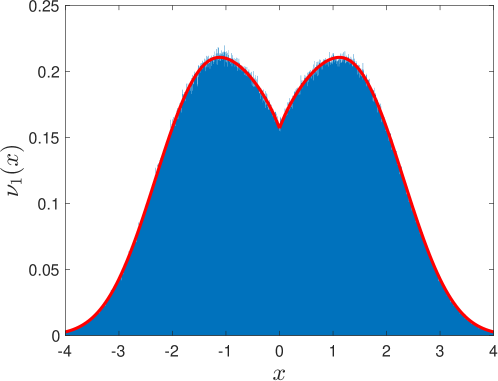
Figure 1: Scaling function for distribution, $\nu_{1}(x)$, eq. (6) curve in red, compared to simulation data where we have saved the index of the final point of a trajectory, blue histogram. The distribution is a function of only $|x|$, and is singular at $x=0$. The empirical distribution has a width of $\sim 7,600$ sites. $t=262,144$ Monte Carlo steps.

We generate data, for the simulation of an elastic chain of $N$ particles linked by harmonic springs. We initialise the chain to its ground state. We then perform $m=13\times 10^{6}$ simulations involving $t=4N$ event-chain steps. We are not sampling from the Boltzmann distribution, rather studying the dynamics, so we do not stop the simulation after a pre-specified chain length as is usually required in event chain sampling. During each simulation, we cumulate the number of visits to each site by the active particle, $L$. At the end of each of the $m$ simulations we save the index of the final active particle (which in the continuum limit corresponds to $x$), as well as the number of visits of the active particle to the final chain position $h$. After the simulation, the data is binned generating empirical distributions, that we compare with eqs. (6, 7). These curves represent probability distributions and are thus automatically normalized to unit area. The only free variable in comparing the analytic expressions to the binned numerical data is thus the choice of the horizontal scale. We fix this one undetermined scale by imposing that the first moment of the empirical curve matches the theoretical expression.

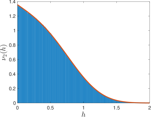
Figure 2: Scaling function for the number of site visits at the end-point of motion, $\nu_{2}(x)$ eq. (7) curve in red, compared to simulation data, blue histogram. Width of distribution is $\sim 19$ sites. Same simulation as Fig. 1

We plot the results of our analysis Fig. 1, for the displacement distribution function $\rho_{1}$, and for the local time distribution $\rho_{2}$, Fig. 2. The solid (red) lines are the analytic expressions. We find excellent agreement between theory and numerics. We note, in particular, that as predicted by theory the distribution of Fig. 1 has a singularity at the origin. We also performed simulations starting from a pre-equilibrated physical system. In this case, we find very similar distributions to those plotted in Figs. 1, 2 with however, a change of scale in the axes, see also [11].

Lifted TASEP

Finally, we perform a numerical study of the lifted TASEP model [17]. We consider a system of $N$ particles on a periodic lattice of length $2N$. We initialise the system in a crystal of equally spaced particles. Simulations on short times give rise to an asymmetric distribution from for $\rho_{1}(x)$ (Fig. 3, top), but longer simulations give a very slow convergence to a more symmetric form (Fig. 3, bottom). We conclude that the lifted TASEP displays very similar phenomenology to the harmonic chain, and is also in the same dynamic universality class as true self-avoiding motion. We also confirmed, for lifted TASEP, the expected scaling of displacement of the activity in $t^{2/3}$, Fig. 4 (top). We note the distribution of displacement is strongly skewed for short simulation times. It is only after a long simulation time that the back-forwards symmetry is established Fig. 4, (bottom). When we start with a configuration which is generated randomly, the initial asymmetry is much weaker, though not zero.

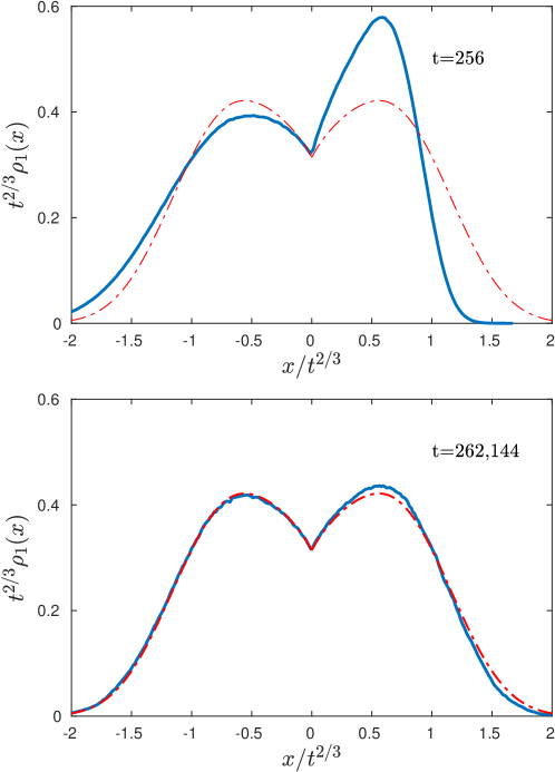
Figure 3: Distribution of displacements of the activity $\rho_{1}(t,x)$, for lifted TASEP. Top, a short simulation of $t=256$ steps generates a skewed distribution. Bottom, a longer time scale of $t=262,144$ generates a distribution which is close to that found in Fig. 1, while still displaying a very slight left-right asymmetry. Scaled curve of $\nu_{1}(x)$ red/dashed.

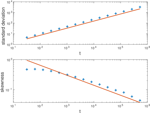
Figure 4: Evolution of moments of $\rho_{1}(t,x)$ for lifted TASEP. Top: standard deviation of the distribution, compared to evolution in $t^{2/3}$. Bottom, skewness (normalized third moment) compared to $t^{-1/3}$. The decrease in skewness corresponds to a distribution which progressively becomes more symmetric.

Conclusions

To conclude, we have presented an argument that the evolution of a system subject to non-reversible Monte Carlo is directly linked to the continuum limit of a growth model [5]. We performed extensive simulations using an event chain algorithm and compared the resulting distributions to those calculated in [10, 11, 19]. We find excellent agreement, for both a harmonic chain, and for the non-harmonic lifted TASEP, and so conclude that the non-reversible algorithm is indeed a realisation of a true self-repelling motion.

Event chain methods, including factor fields, have been generalized to higher dimensions [20]. It would be of interest to transfer the formalism of the present paper to such systems, with the aim of better understanding the algorithmic limits of even-chain methods.

The code used to simulate the two physical systems, as well as the analysis code is available from the author.

References

- [1] Bernard E P, Krauth W and Wilson D B 2009 Phys. Rev. E 80(5) 056704 URL https://link.aps.org/doi/10.1103/PhysRevE.80.056704
- [2] Michel M, Kapfer S C and Krauth W 2014 The Journal of Chemical Physics 140 054116 ISSN 0021-9606 (Preprint https://pubs.aip.org/aip/jcp/article-pdf/doi/10.1063/1.4863991/15472076/054116_1_online.pdf) URL https://doi.org/10.1063/1.4863991
- [3] Harland J, Michel M, Kampmann T A and Kierfeld J 2017 Europhysics Letters 117 30001 URL https://dx.doi.org/10.1209/0295-5075/117/30001
- [4] Faulkner M F, Qin L, Maggs A C and Krauth W 2018 The Journal of Chemical Physics 149 064113 ISSN 0021-9606 (Preprint https://pubs.aip.org/aip/jcp/article-pdf/doi/10.1063/1.5036638/13501056/064113_1_online.pdf) URL https://doi.org/10.1063/1.5036638
- [5] Amit D J, Parisi G and Peliti L 1983 Phys. Rev. B 27(3) 1635–1645 URL https://link.aps.org/doi/10.1103/PhysRevB.27.1635
- [6] Bernasconi J and Pietronero L 1984 Phys. Rev. B 29(9) 5196–5198 URL https://link.aps.org/doi/10.1103/PhysRevB.29.5196
- [7] Pietronero L 1983 Phys. Rev. B 27(9) 5887–5889 URL https://link.aps.org/doi/10.1103/PhysRevB.27.5887
- [8] Obukhov S P and Peliti L 1983 Journal of Physics A: Mathematical and General 16 L147 URL https://dx.doi.org/10.1088/0305-4470/16/5/004
- [9] Tóth B and Werner W 1998 Probability Theory and Related Fields 111 375–452 URL https://doi.org/10.1007/s004400050172
- [10] Tóth B 1995 The Annals of Probability 23 1523 – 1556 URL https://doi.org/10.1214/aop/1176987793
- [11] Dumaz L and Tóth B 2013 Stochastic Processes and their Applications 123 1454–1471 ISSN 0304-4149 URL https://www.sciencedirect.com/science/article/pii/S0304414912002517
- [12] NIST Digital Library of Mathematical Functions https://dlmf.nist.gov/, Release 1.1.11 of 2023-09-15 f. W. J. Olver, A. B. Olde Daalhuis, D. W. Lozier, B. I. Schneider, R. F. Boisvert, C. W. Clark, B. R. Miller, B. V. Saunders, H. S. Cohl, and M. A. McClain, eds. URL https://dlmf.nist.gov/
- [13] Kapfer S C and Krauth W 2017 Phys. Rev. Lett. 119(24) 240603 URL https://link.aps.org/doi/10.1103/PhysRevLett.119.240603
- [14] Lei Z and Krauth W 2018 Europhysics Letters 121 10008 URL https://dx.doi.org/10.1209/0295-5075/121/10008
- [15] Lei Z, Krauth W and Maggs A C 2019 Phys. Rev. E 99(4) 043301 URL https://link.aps.org/doi/10.1103/PhysRevE.99.043301
- [16] Derrida B 1998 Physics Reports 301 65–83 ISSN 0370-1573 URL https://www.sciencedirect.com/science/article/pii/S0370157398000064
- [17] Essler F H L and Krauth W 2023 Lifted TASEP: a Bethe ansatz integrable paradigm for non-reversible Markov chains (Preprint 2306.13059)
- [18] Peierls R 1935 Annales de l’institut Henri Poincaré 5 177–222 URL http://www.numdam.org/item/AIHP_1935__5_3_177_0/
- [19] Tóth B 2001 Self-interacting random motions European Congress of Mathematics ed Casacuberta C, Miró-Roig R M, Verdera J and Xambó-Descamps S (Basel: Birkhäuser Basel) pp 555–564 ISBN 978-3-0348-8268-2
- [20] Maggs A C and Krauth W 2022 Physical Review E 105 URL https://doi.org/10.1103%2Fphysreve.105.015309