Spatial information allows inference of the prevalence of direct cell-to-cell viral infection

Abstract

The role of direct cell-to-cell spread in viral infections — where virions spread between host and susceptible cells without needing to be secreted into the extracellular environment — has come to be understood as essential to the dynamics of medically significant viruses like hepatitis C and influenza. Recent work in both the experimental and mathematical modelling literature has attempted to quantify the prevalence of cell-to-cell infection compared to the conventional free virus route using a variety of methods and experimental data. However, estimates are subject to significant uncertainty and moreover rely on data collected by inhibiting one mode of infection by either chemical or physical factors. These methods assume that this inhibition process fully eliminates its target mode of infection while exactly preserving the dynamics of the other. In this work, we provide a framework for estimating the prevalence of cell-to-cell infection from data which is experimentally obtainable without the need for additional interventions, and two standard mathematical models for viral dynamics with the two modes of infection. We provide guidance for the design of relevant experiments and mathematical tools for accurately inferring the prevalence of cell-to-cell infection.

Keywords: Cell-to-cell viral infection, viral dynamics, Bayesian inference, multicellular model, agent-based model.

Introduction

Classically, viral infections have been assumed to spread among host cells through a process of viral secretion, diffusion, and reabsorption via the extracellular environment [10, 8]. In reality, however, a huge variety of the most medically important viruses — including influenza A, herpesviruses, hepatitis C, HIV and SARS-CoV-2 — have all been observed to also spread between host cells using direct cell-to-cell mechanisms [14, 12, 24]. This mode of infection, which is mechanistically distinct from the conventional cell-free route, permits viruses or viral proteins to be trafficked directly between adjacent cells without ever being leaving the cell membrane [12]. This is significant for multiple reasons. For one, the direct cell-to-cell route of infection is orders of magnitude more efficient than the cell-free route [13, 9], and moreover is far better protected from immune or drug defences [13, 19, 24]. Cell-to-cell infection is considered one of the essential strategies of chronic viral infections like hepatitis C and HIV, and elevated cell-to-cell spread has been associated with increased pathogenicity in influenza and SARS-CoV-2 infections [13, 27]. Understanding the role and prevalence of cell-to-cell infection in different viral species is therefore of profound importance in therapeutic applications.

Recent works, both from the modelling and experimental literature, have made efforts to identify the prevalence of the cell-to-cell mode of viral infection. In hepatitis C, modelling efforts led by Graw and Durso-Cain suggested that cell-free infection events were rare, yet worked synergistically with the cell-to-cell infection strategy to rapidly accelerate the overall rate of infection spread [9, 5]. Blahut and coworkers used modelling to quantify the proportion of the two modes of spread using in vitro experimental data, and claimed that as much as 99% of the infection events observed were due to cell-to-cell infection [2]. Experimental work by Kongsomros and colleagues suggested that the proportion of cell-to-cell infections in influenza was very low, but elevated in more pathogenic strains of the virus [13]. By contrast, experimental work in SARS-CoV-2 by Zeng and collaborators claimed that cell-to-cell infection represented around 90% of infections [27].

These estimates in the literature for cell-to-cell prevalence among different viruses are in sparse supply, and subject to significant uncertainty. Moreover, to our knowledge, all share a common limitation, being that they rely on experiments which knock out only one of the modes of viral spread, usually cell-free infection, and leaves the other infection mechanism untouched [2, 13, 27]. This is usually implemented by conducting infection assays in the presence of an antiviral such as oseltamivir for influenza, or by imposing a physical barrier to viral diffusion, such as treating the cell sheet with methylcellulose [13, 27]. However, it is not known whether these additional experimental controls increase or decrease the productivity of the cell-to-cell infection route.

To our knowledge, only one publication in the literature has attempted to infer the balance of the two modes of infection spread from data where both mechanisms are unimpeded [15]. This work, by Kumberger and colleagues, demonstrates modifications that can be made to a standard ordinary differential equation (ODE) model of viral dynamics in order to better describe cell-to-cell infection, but was nonetheless unable to satisfactorily infer the prevalence of cell-to-cell infection from synthetic data where the two modes of infection occurred simultaneously, and moreover did not examine whether estimates of this quantity were improved or weakened when the true balance of the two mechanisms was changed [15]. The limits of identifiability of the proportion of cell-to-cell infection — under different conditions, using different models, and based on different sources of observational data — has not been systematically studied.

Here, we conduct simulation estimation studies using two mathematical models for viral infections with two modes of spread: one non-spatial ODE system and one spatially-explicit multicellular model. In both cases, we generate synthetic data using the model in combination with an observational model, and attempt to re-estimate the prevalence of cell-to-cell infection from the resulting observations. We repeat this process under a range of conditions and with different types of available data for fitting. Our results provide an important background for the identifiability of the cell-to-cell infection prevalence, and offer guidance for the design of models and experimental systems best equipped to learn this quantity.

In this work we take particular inspiration from the work of Kongsomros and colleagues [13]. In their work, the authors conduct a series of experiments where “donor” cells infected with influenza are added to a well of “recipient” cells, labelled with a membrane dye, and infection allowed to spread under a given set of experimental conditions. At various times, wells are harvested and fixed, then stained with fluorescent anti viral-NP antibody to identify the infected recipient cell population. In the present work, we will take the fluorescent cell proportion, following the construction given here, as our primary source of observational data. We provide further discussion of our choice of data source in Discussion.

Results

In the presence of observational noise, the prevalence of cell-to-cell infection spread cannot be determined from fluorescence time series data alone

We sought to investigate whether an ODE model incorporating both cell-free viral infection and cell-to-cell infection, could be used to infer the balance of the two modes of spread, given a time series of observations of the fluorescent proportion of the cell population as in Kongsomros et al. [13]. We exhibit the basic properties of the ODE model in Figure 1 (the model is fully described in Methods “An ODE model for dual-spread dynamics”). Figure 1(a) shows the basic structure of the model and the parameters governing the model. We apply a standard target cell-limited model framework with a latent compartment and two modes of infection. That is, initially susceptible cells may become infected either through cell-to-cell infection — at a rate proportional to the infected proportion of the cell population — or through infection by cell-free virus — at a rate proportional to the quantity of extracellular virus in the system. Once initially infected, cells enter the first of $K$ eclipse stages (such that the duration of the eclipse stage is gamma-distributed, instead of exponentially-distributed, see [21, 6]), before becoming productively infected, at which stage they begin producing extracellular virus. Productively infected cells then die. We assume that cells become detectably fluorescent once they become productively infected, but that they remain fluorescent after death over the time scale of simulations, as observed in Kongsomros et al. [13].

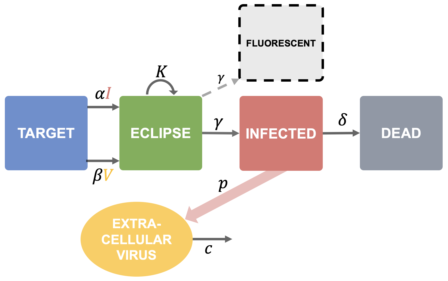
(a)

r27ptt19pt

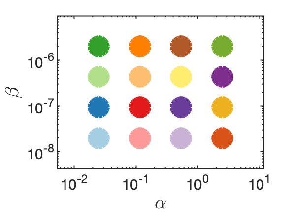
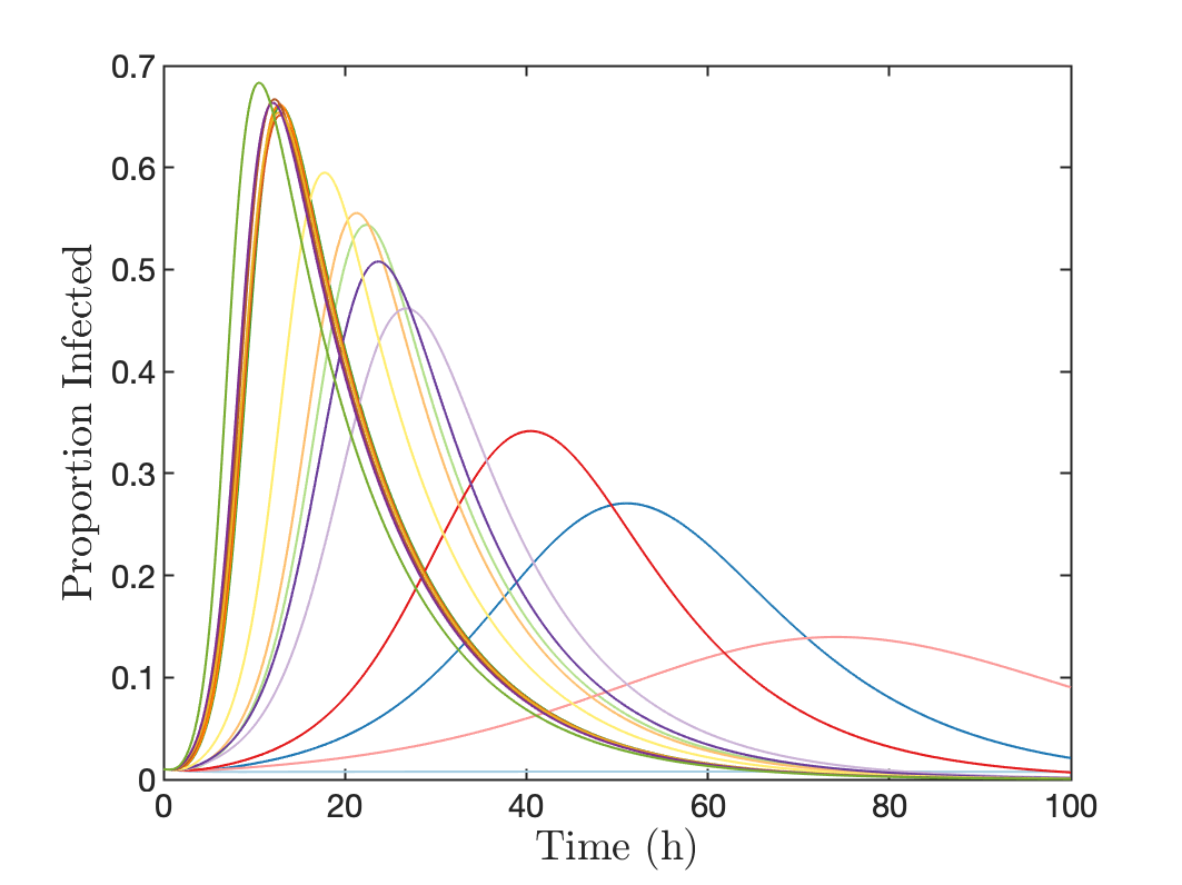
(b)

r25ptb55pt

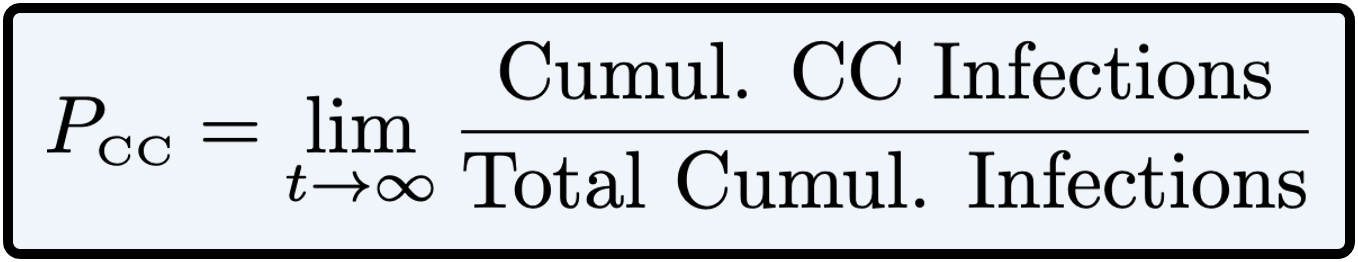
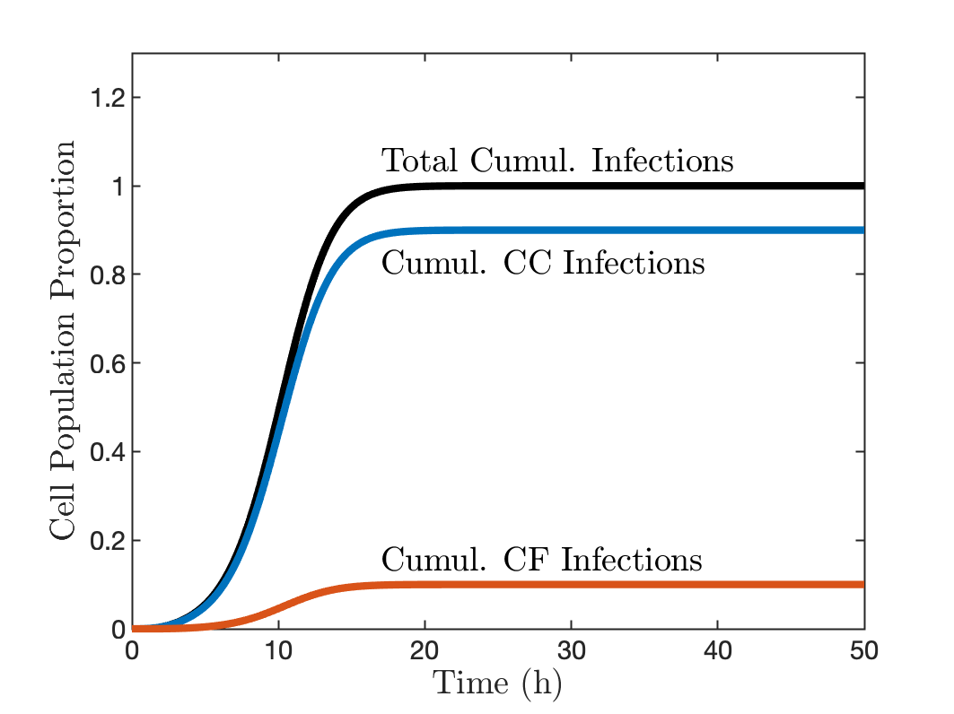
(c)

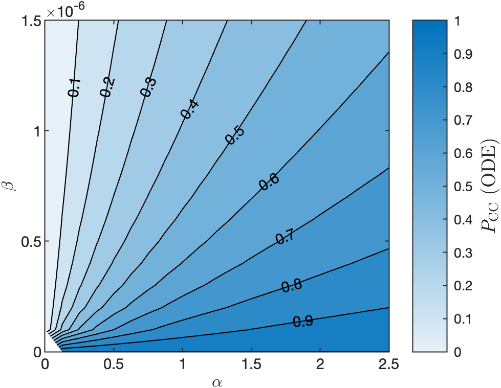
(d)

Figure 1: (a) Schematic of the ODE model. (b) Proportion of infected cells over time as predicted by the ODE model for an array of values of $\alpha$ and $\beta$ between zero and 2.5 and 2$\times 10^{-6}$, respectively. The parameter values sampled to generate the plot are shown in the inset. (c) Calculation of $P_{\text{\tiny CC}}$. We keep track of the proportion of the cell population which has been infected by the cell-to-cell (CC) and cell-free (CF) infection over the course of infection. We define $P_{\text{\tiny CC}}$ as the proportion of infections arising from the CC route at long time. (d) $P_{\text{\tiny CC}}$ contour map on $\alpha$–$\beta$ space for the dual-spread ODE model. $\alpha$ and $\beta$ have units of $\text{h}^{-1}$ and $\text{(TCID}_{50}\text{/ml)}^{-1}\text{h}^{-1}$, respectively.

Throughout this work we will take the majority of the model parameters to be fixed (which is discussed in Section Methods “An ODE model for dual-spread dynamics”), aside from the two parameters governing the rates of cell-to-cell and cell-free infection, $\alpha$ and $\beta$, respectively. Figure 1(b) shows the dynamics of the infected cell proportion over time using the ODE model with a range of $\alpha$ and $\beta$ values (throughout this work, $\alpha$ and $\beta$ have units of $\text{h}^{-1}$ and $\text{(TCID}_{50}\text{/ml)}^{-1}\text{h}^{-1}$, respectively). We can quantify and describe the overall rate of infection progression by the exponential growth rate $r$ (units of $\text{h}^{-1}$). This quantity, well established in the theory of both between-host and within-host infection dynamics, describes the initial rate of exponential expansion of the infected (or fluorescent) population [3, 17]. For further details refer to Methods “Exponential growth rate - $r$”.

We applied simulation estimation techniques to investigate whether $\alpha$ and $\beta$ could be inferred from the fluorescent cell time series of the model. We first selected three sets of $(\alpha,\beta)$ pairs resulting in different proportions of infections arising from each mechanism. Specifically, if we label the final fraction of infections arising from the cell-to-cell route as $P_{\text{\tiny CC}}$, we construct lookup tables on $\alpha$–$\beta$ space for this quantity, and use this to compute $(\alpha,\beta)$ pairs corresponding to $P_{\text{\tiny CC}}$ values of approximately 0.1, 0.5, and 0.9, with a fixed exponential growth rate $r$ of 0.52 in each case to ensure the overall dynamics progressed at a comparable rate. We show a graphic of the computation of $P_{\text{\tiny CC}}$ in Figure 1(c), and a contour map on $\alpha$–$\beta$ space for the ODE model in Figure 1(d). For further details on $P_{\text{\tiny CC}}$, refer to Methods “Proportion of infections from the cell-to-cell route - $P_{\text{\tiny CC}}$”.

For each of the specified values of $(\alpha,\beta)$, we simulated the ODE model and, following Kongsomros and colleagues, we computed the fluorescent cell proportion $F(t)$ — that is, the cumulative proportion of the initially susceptible population that has become infected — at $\mathbf{t}=\left\{3,6,9,...,30\right\}$h [13]. We then applied an observational model to this data to simulate the experimental process, by assuming a cell population size $N_{\text{\tiny sample}}$, and overdispersed noise modelled by a negative binomial distribution. We take $N_{\text{\tiny sample}}=2\times 10^{5}$ as in [13] and set the dispersion parameter $\phi=10^{2}$, selected to impose a modest amount of noise on our observations, leading to the observed data vector $\mathbf{D}$. We specify the observation model in full in Methods “Simulation estimation”, and explore the role of observational noise in more detail in Supplementary Section 1.

Having obtained our observed data $\mathbf{D}$, we run a No U-Turn Sampling (NUTS) Markov Chain Monte Carlo (MCMC) algorithm [23] to obtain posterior density estimates for $\alpha$ and $\beta$. For each $(\alpha,\beta)$ pair to estimate, we run ten replicates — that is, we repeat the process of applying observational noise to the true fluorescence data and re-estimating $\alpha$ and $\beta$ ten times — and for each replicate we use four independent and randomly seeded chains. We assume uniform priors for $\alpha$ and $\beta$ on $\left[0,5\right]\text{h}^{-1}$ and $\left[0,1\times 10^{-5}\right]\text{(TCID}_{50}\text{/ml)}^{-1}\text{h}^{-1}$ respectively, and assume a negative binomial likelihood. Further details of this simulation estimation process are specified in Methods “Simulation estimation”.

In Figure (2), we show the results of this fitting process. In Figures 2(a)–2(c), we show posterior samples in $(\alpha,\beta)$ space from each chain of a single replicate fit. We do so for each of the three target parameter pairs. As a visual aid, we also plot the $(\alpha,\beta)$ contours corresponding to the true $P_{\text{\tiny CC}}$ value and the true $r$ value in each case. These plots confirm that the chains are indeed well-mixed, however, they also show that the posterior samples for each pair of target parameters are spread out along the true $r$ contour. While some samples are close to the target parameter pair, the chains do not appear to converge at this point. This is confirmed in Figure 2(d). In Figure 2(d), for each target parameter pair, we show violin plots of the posterior distributions of $P_{\text{\tiny CC}}$ and $r$ for four replicate fits, along with a box plot of the posterior medians across all ten replicates. We also show the prior density of both of these quantities in grey. Figure 2(d) shows that while $r$ is well estimated compared to its prior distribution — regardless of the choice of target parameters — $P_{\text{\tiny CC}}$ cannot be identified. Whilst, at least for the case where the target $P_{\text{\tiny CC}}=0.1$, the distribution of posterior medians can be somewhat accurate, posterior distributions from individual replicates are frequently far from the true value. Importantly, many of these posterior distributions are reasonably confident, yet also wrong, for instance, Replicate 4 for the case where the target $P_{\text{\tiny CC}}=0.5$. Overall, this experiment indicates that, when even a modest degree of observational noise is applied to the fluorescence data, only the exponential growth rate $r$ can be accurately estimated: the proportion of infections arising from each mode of spread is lost in the observational process.

FITTING FLUORESCENCE DATA – ODE MODEL

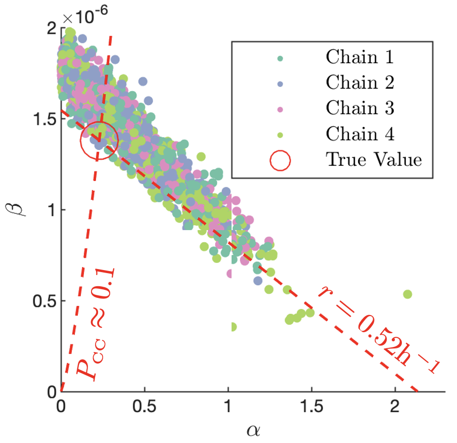
(a)

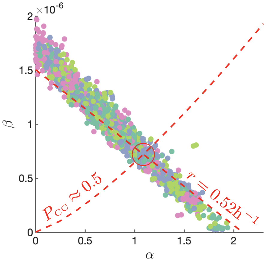
(b)

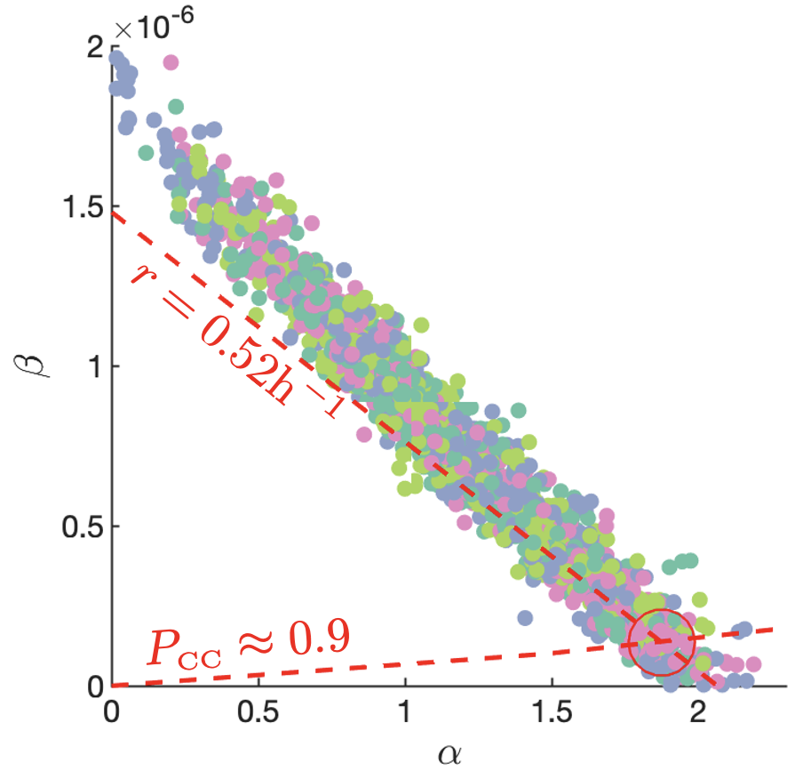
(c)

(d)

Figure 2: (a)–(c) MCMC chains in $\alpha$–$\beta$ space for a fit to fluorescence data with typical observational noise where the true $P_{\text{\tiny CC}}\approx$ 0.1, 0.5, 0.9 and the value of $r$ is held fixed. (d) Prior density and posterior densities from individual replicates for $r$ and $P_{\text{\tiny CC}}$ both with typical observational noise. We repeat this for three sets of parameters resulting in $P_{\text{\tiny CC}}$ values of 0.1, 0.5 and 0.9 with a fixed $r$ value. Dashed and solid horizontal lines mark the mean and median values respectively. We also show a box plot of the distribution of posterior medians across all replicates. There are ten replicates in total at each value of $P_{\text{\tiny CC}}$, of which we display four. $\alpha$ and $\beta$ have units of $\text{h}^{-1}$ and $\text{(TCID}_{50}\text{/ml)}^{-1}\text{h}^{-1}$, respectively.

We investigated the role of the level of observational noise in determining the quality of estimates of $P_{\text{\tiny CC}}$ and $r$ using the ODE model (for full details, see Supplementary Section 1). We found that for higher values of the dispersion parameter $\phi$ than we show here (that is, with less observational noise), estimates of $P_{\text{\tiny CC}}$ were overall closer to the true value, however, the distribution of estimate medians still showed not insignificant variance, even when virtually all observational noise was removed. Subject to a higher level of observational noise, estimates of $P_{\text{\tiny CC}}$ were almost entirely random. We show these results in full in Supplementary Figure SI 1.

Using a spatial model with spatial data, the balance of the modes of infection spread can be accurately inferred

We sought to apply a similar simulation estimation procedure to a spatially-structured model of infection, to investigate whether a model capable of describing the actual structure of infection would provide better estimates of the proportion of each infection mechanism. We constructed an agent-based spatial model with an equivalent structure to the ODE model used in the previous result, where transitions between compartments of the model are replaced by probabilities of discrete cells, occupying specific positions in space, changing between states analogous to those in the ODE model. The notable difference in this construction is that while we still model cell-free infection based on a global extracellular viral reservoir, we now model cell-to-cell infection as a spatially local process. Specifically, we assume that the probability of cell-to-cell infection of a given cell is based on the infected proportion of its neighbours, instead of the global infected cell population as in the ODE model. This reflects the assumption — based on current biological understanding — that cell-free virions spread rapidly over the size of tissue we seek to model, whereas cell-to-cell infection is possible only between adjacent cells [14]. This process is illustrated in Figure 3(a). Figure 3(a) shows a schematic of the spatial model, and illustrates the alternate formulation of the cell-to-cell infection mode. Note that, as illustrated in the schematic, cells are packed in a hexagonal lattice, which reflects the biological reality of epithelial monolayers and moreover ensures that adjacency between cells is well-defined. Full details of the spatial model can be found in Methods “A multicellular spatial model for dual-spread dynamics”.

In addition to the fluorescent proportion metric we introduced in the previous result, we developed an additional metric for the spatial model to describe the extent to which infected cells were clustered together. This metric, which we term $\kappa(t)$, describes the mean proportion of neighbours of the fluorescent cells which are also fluorescent at time $t$. In Figure 3(c) we show a schematic which illustrates the computation of the fluorescent neighbour fraction at a number of fluorescent cells in a cell sheet. We define $\kappa(t)$ explicitly in Methods “Clustering metric - $\kappa(t)$”. $\kappa(t)$ has the property that when it is large, fluorescent cells tend to be clustered together and the infection is highly localised, whereas if it is small, the infection is diffuse.

In Figure 3(d)–3(g), we demonstrate the behaviour of the spatial model under three $(\alpha,\beta)$ parameter pairs, chosen to result in a $P_{\text{\tiny CC}}$ of approximately 0.1, 0.5, and 0.9, and to reach a peak infected cell fraction at approximately $18\text{h}$. In Figure 3(d), we visualise a section of the cell grid at a series of time points. We do so by assigning a unique index $j=\left\{1,2,...,N_{\text{\tiny init}}\right\}$ to each of the $N_{\text{\tiny init}}$ initially infected cells and the extracellular virus they produce. Then, every time a susceptible cell is marked for infection during a simulation, we compute the probability that it was caused by each of the $N_{\text{\tiny init}}$ viral lineages, and determine the lineage assigned to that cell. Infected cells are then coloured by their lineage. Once a cell dies, we change its colour to black. This construction allows us to visualise the spread of infection in space. Figure 3(d) shows that when cell-to-cell infection dominates, infection plaques are tightly clustered and infected cells of the same lineage tend to be found closer together. When cell-free infection dominates, there is no particular structure to the colouring of the cell sheet. In Figure 3(e)–3(g), we show time series for the spatial model under the same three parameter schemes as discussed above: the proportion of the cell population which is infected over time, the fluorescent cell curve as discussed in the previous section, and the clustering metric $\kappa(t)$. These time series indicate that even though the different parameter regime lead to vastly differently-structured infections — as can be seen in Figure 3(d) — their infected and fluorescent cell count dynamics as a time series are relatively similar, although there is some variation in the initial uptick of infection in the case where $P_{\text{\tiny CC}}$ is large. By contrast, the time series for $\kappa(t)$ shows substantial variation between the parameter values corresponding to low, roughly equal and high values of $P_{\text{\tiny CC}}$.

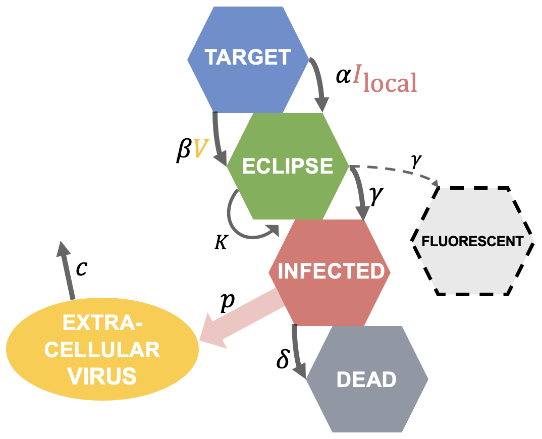
(a)

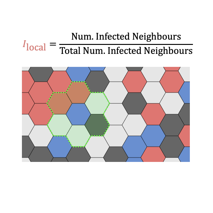
(b)

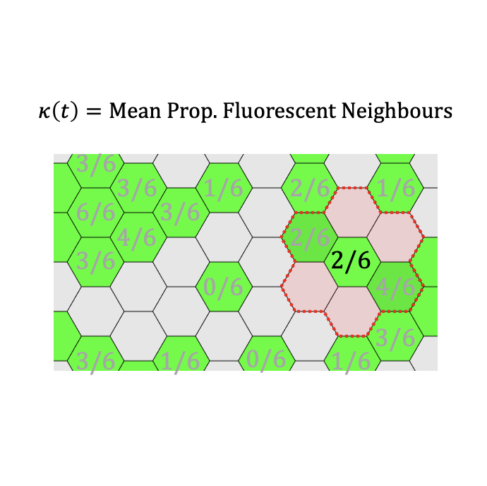
(c)

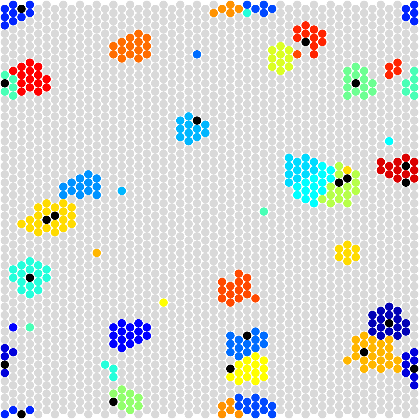
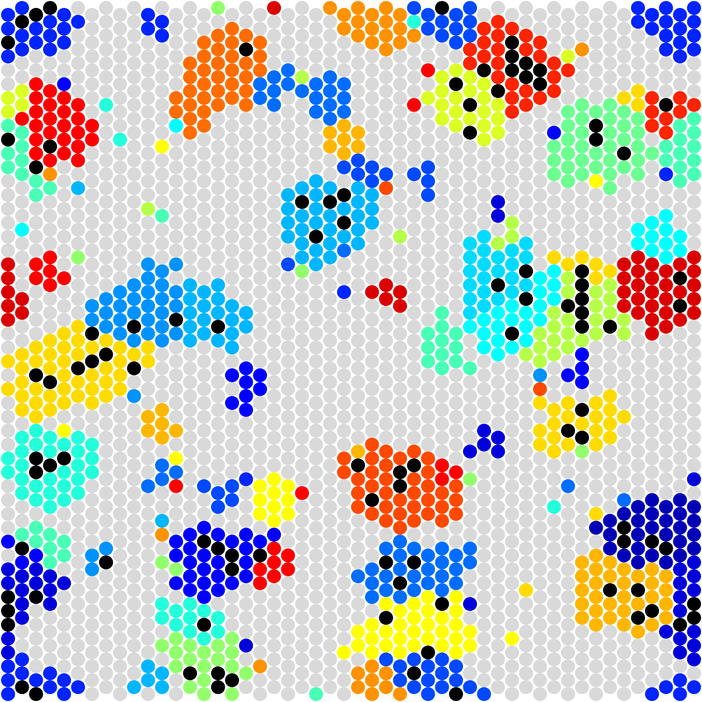
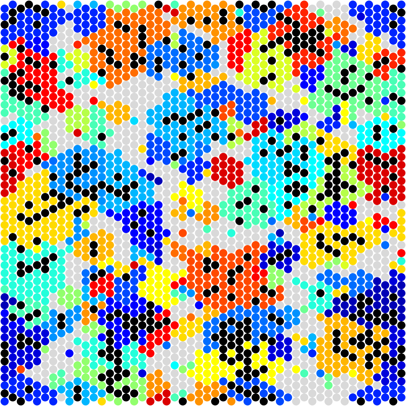
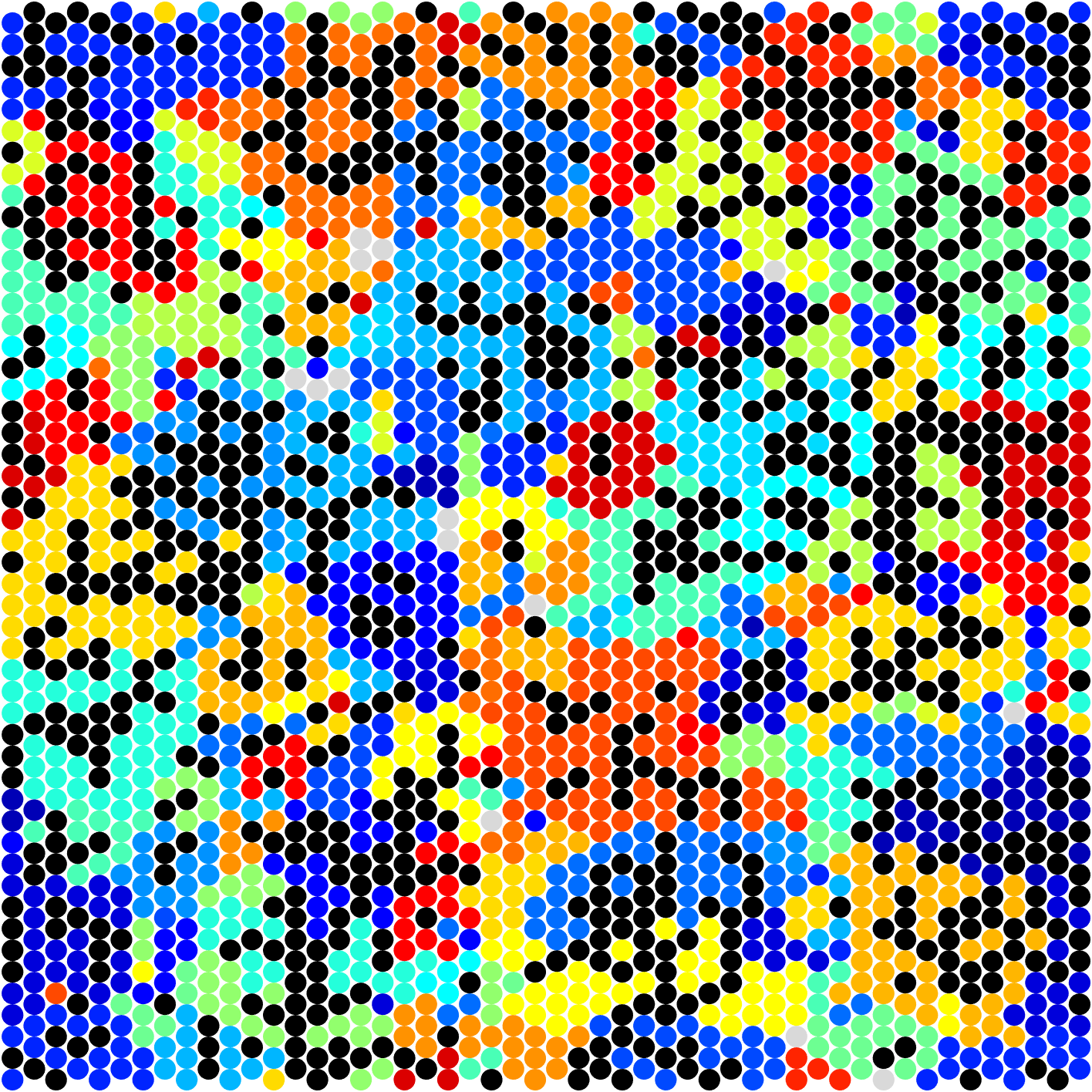
	$t=0h$	$t=4h$	$t=8h$	$t=12h$	$t=16h$

(d)

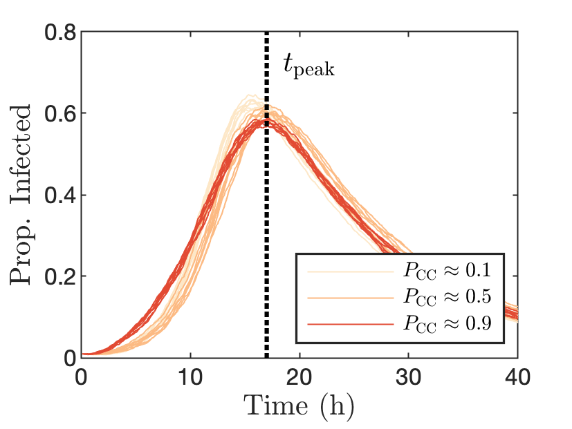
(e)

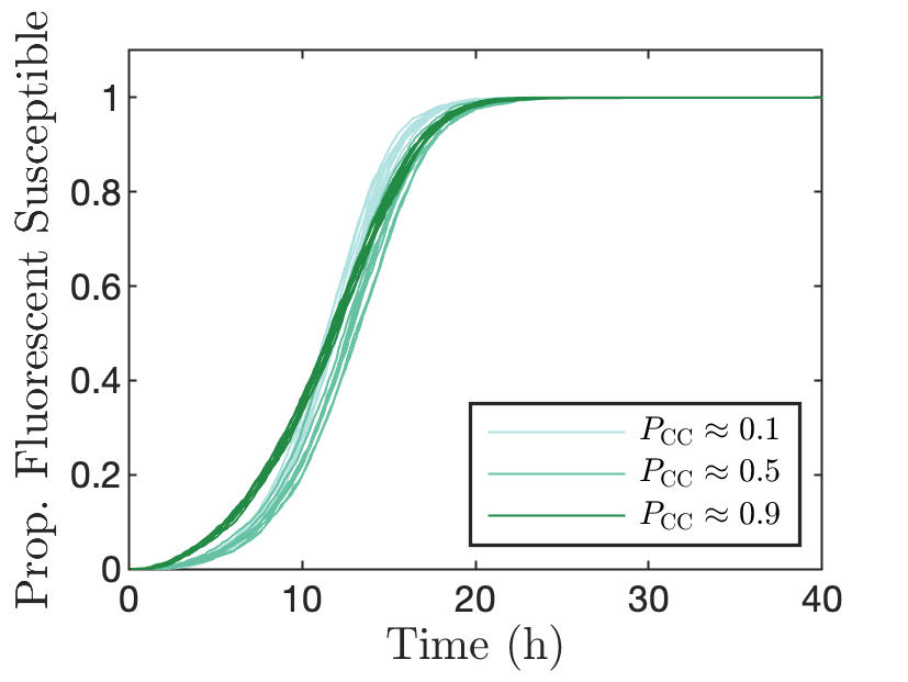
(f)

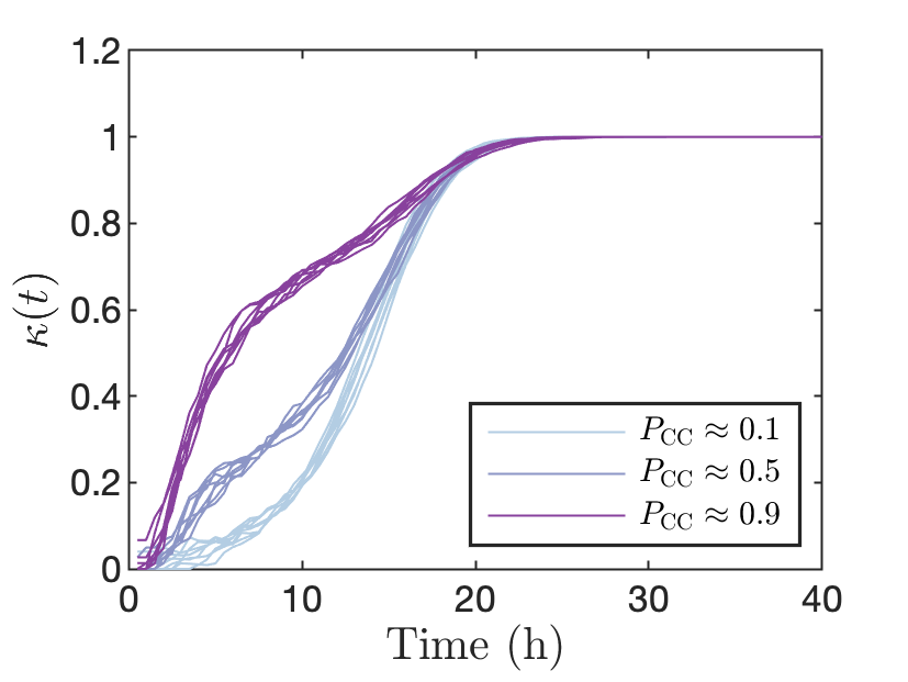
(g)

Figure 3: (a) Schematic of the spatial model. The model follows the same structure as the ODE model with the exception that cell-to-cell infection is based on the proportion of a cells neighbours which are infected. (b) Cartoon of the calculation of infected neighbour proportion. (c) $\kappa(t)$ is our clustering metric, computed as the mean proportion of neighbours of the fluorescent cells which are also fluorescent. (d) Typical time evolution of the cell grid using the spatial model under three $\alpha$–$\beta$ combinations, resulting in $P_{\text{\tiny CC}}$ values of approximately 0.1, 0.5, and 0.9. Parameters were chosen such that the peak infected cell population is reached at approximately the same time in each instance. Initially infected cells are flagged with a unique colour and infections resulting from that lineage of cells are assigned the same colour. Target cells are marked in grey and dead cells in black. (e), (f), (g) Proportion of cell sheet infected, proportion of susceptible cells which are fluorescent over time, and the clustering metric $\kappa(t)$ respectively. We show eight simulations for each of the $\alpha$–$\beta$ parameter pairs described above. $\alpha$ and $\beta$ have units of $\text{h}^{-1}$ and $\text{(TCID}_{50}\text{/ml)}^{-1}\text{h}^{-1}$, respectively.

Since in the spatial model, cell-to-cell infection is constrained to act locally, infections that spread mainly through cell-to-cell infection are forced to spread radially. The size of the resulting infected cell population, therefore, grows in a non-exponential manner. For this reason, the exponential growth rate $r$ is not well-defined in the case of the spatial model. As an alternative metric of the rate of growth of the infected cell population, we simply use the time of the peak infected cell population, which we label as $t_{\text{\tiny peak}}$. Since this, like $P_{\text{\tiny CC}}$, cannot be well-estimated a priori, we again resort to computing a lookup table of mean $t_{\text{\tiny peak}}$ values on $\alpha$–$\beta$ space. For full details on the construction of these lookup tables and their corresponding surface plots, refer to Methods “Proportion of infections from the cell-to-cell route - $P_{\text{\tiny CC}}$” and Figures 6(a)–6(b).

We computed $(\alpha,\beta)$ pairs for the spatial model which result in $P_{\text{\tiny CC}}$ values of approximately 0.1, 0.5, and 0.9 and a common value of $t_{\text{\tiny peak}}$ of approximately 18h, analogous to the values selected for the ODE model in our previous fitting experiment. For each of these parameter pairs, we ran simulations of the spatial model and reported the fluorescent proportion of the susceptible cells as well as the clustering metric $\kappa(t)$ at times $\mathbf{t}=\left\{3,6,9,...,30\right\}$h, one time point per simulation. This model reflects the destructive experimental observation process. We provide full details of the observational model in Methods “Simulation estimation”. The resulting observations collectively form our observed data vectors $\mathbf{D}^{\text{\tiny fluoro}}$ and $\mathbf{D}^{\text{\tiny cluster}}$. We then used Population Monte Carlo (PMC) methods to re-estimate $\alpha$ and $\beta$ (full details in Methods “Simulation estimation”) given this synthetic observational data. For each of the three target $(\alpha,\beta)$ pairs, we ran four replicates of the data generation and fitting process.

We show the results of this experiment in Figure 4. Figure 4, which follows a similar layout to Figure 2, shows that with the addition of clustering metric data, $P_{\text{\tiny CC}}$ can now be robustly inferred using the spatial model. In Figure 4(a)–4(c), we plot scatter plots of the final accepted posterior samples for $\alpha$ and $\beta$ in $\alpha$–$\beta$ space for the three target parameter pairs, resulting in $P_{\text{\tiny CC}}\approx 0.1,~{}0.5,~{}0.9$. These plots show posterior density distributed compactly around the true values of $(\alpha,\beta)$, instead of being dispersed along a $t_{\text{\tiny peak}}$ contour as in the previous simulation estimation. In Figure 4(d), we show the weighted posterior distributions of $P_{\text{\tiny CC}}$ and $t_{\text{\tiny peak}}$ for individual replicates along with the distribution of weighted posterior means across replicates. As before, $t_{\text{\tiny peak}}$ is still extremely well estimated in each case, however, now the posterior distributions for $P_{\text{\tiny CC}}$ are also very accurate to the true value. Moreover, the posterior distributions for individual replicates are concentrated on the true values of $P_{\text{\tiny CC}}$ with only modest confidence intervals, and the distributions of weighted mean estimates across replicates are extremely precise to the true values, meaning that carrying out inference with only a single data stream (as opposed to aggregating across multiple observations) was sufficient to estimate both $P_{\text{\tiny CC}}$ and $t_{\text{\tiny peak}}$. This was not the case with the ODE model. We note that estimates for $P_{\text{\tiny CC}}$ are especially sharp when the true value of $P_{\text{\tiny CC}}$ is higher, suggesting that the dynamics in this high cell-to-cell scheme are particularly distinguishable.

FITTING FLUORESCENCE AND CLUSTERING DATA – SPATIAL MODEL

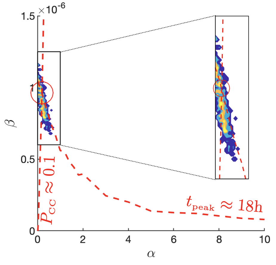
(a)

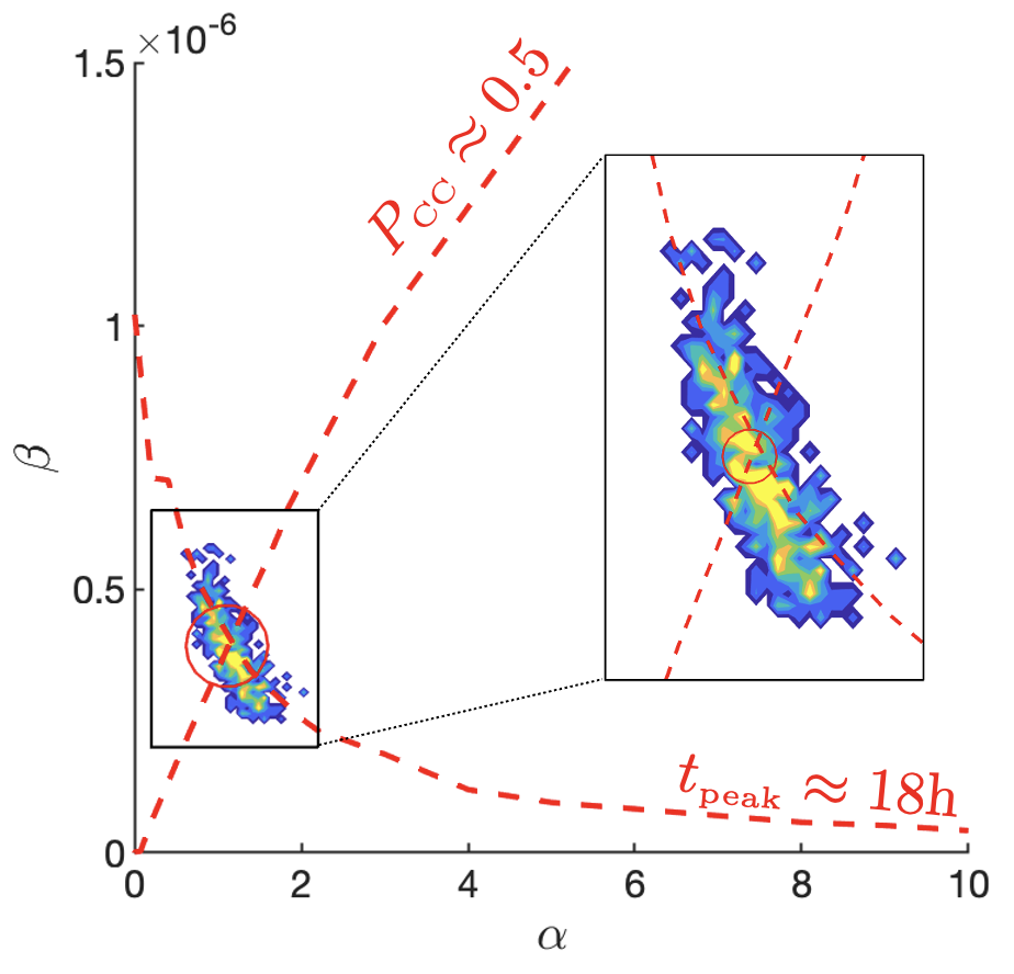
(b)

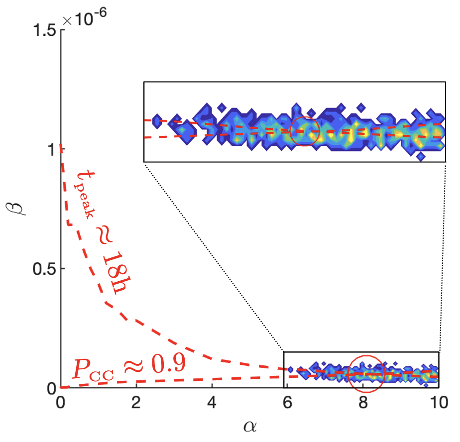
(c)

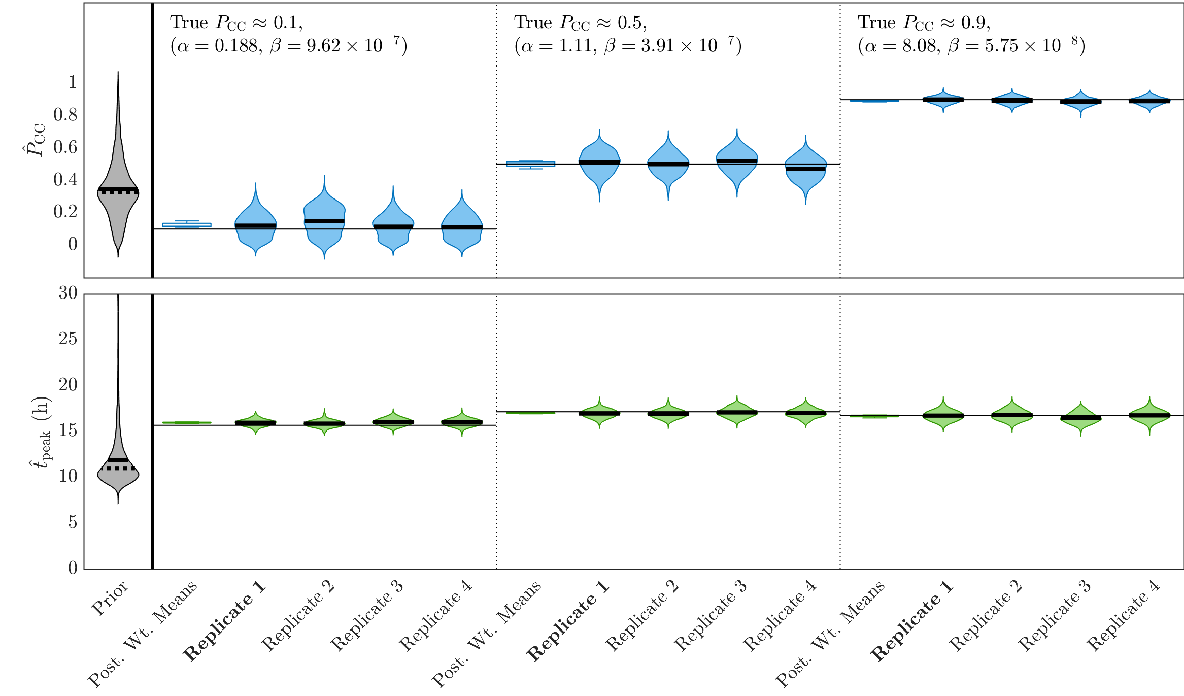
(d)

Figure 4: (a)–(c) Posterior density as a contour plot in $\alpha$–$\beta$ space for a fit to fluorescence and clustering data where the true $P_{\text{\tiny CC}}\approx$ 0.1, 0.5, 0.9 and the infected cell peak time is held fixed at approximately 18h. We only show densities above a threshold value of $10^{-4}$. (d) Prior density and posterior densities from individual replicates for infected peak time ($t_{\text{\tiny peak}}$) and $P_{\text{\tiny CC}}$ with target parameters as specified in (a)–(c). Dashed and solid horizontal lines mark the weighted mean and median values respectively. We also show a box plot of the distribution of posterior weighted means across all four replicates in each case. The replicates in bold are those plotted in (a)–(c). $\alpha$ and $\beta$ have units of $\text{h}^{-1}$ and $\text{(TCID}_{50}\text{/ml)}^{-1}\text{h}^{-1}$, respectively.

To test whether our results were dependent on the inclusion of the secondary data source, the clustering metric $\kappa(t)$, we performed another set of simulation estimations using the same methods as above, this time using only the fluorescence data (full details in Supplementary Section 3). We show the results of this fitting experiment in Supplementary Figure 2. This figure shows that, without the use of the clustering metric, estimates for $P_{\text{\tiny CC}}$ are again very poor, while estimates for $t_{\text{\tiny peak}}$ remain reasonably precise. This result, which mirrors what we observed with the ODE model, suggests that fluorescence data alone is not sufficient to imply the balance of the two modes of viral spread even for the spatial model. We provide more discussion of this in Supplementary Section 3.

Inference on the prevalence of cell-to-cell infection is robust to smaller samples of the cell sheet

The clustering metric $\kappa(t)$, as we have defined it, relies on sampling every fluorescent cell in the tissue at each observation time and calculating the proportion of its neighbours which are also fluorescent. However, in an experimental setting, it may be impractical if not impossible to observe the fluorescent state of every cell in the target population, especially in vivo. We sought to investigate whether approximations of $\kappa(t)$ generated by sampling from subsets of the cell population would be sufficient to allow $\alpha$ and $\beta$ — and therefore $P_{\text{\tiny CC}}$ — to be inferred. We did so by carrying out simulation estimations as in the previous result, but where the clustering metric is now approximated by $\kappa_{S}(t)$, which is computed by randomly sampling $S$ cells instead of sampling the entire grid. Full details of this adjusted simulation estimation process are given in Methods “Clustering metric - $\kappa(t)$”.

To test the influence of the sample size $S$ on estimation of $P_{\text{\tiny CC}}$, we performed a series of simulation estimations on the spatial model using both fluorescence and approximate clustering data for varying sample sizes and target values of $P_{\text{\tiny CC}}$. These simulation estimations were conducted using the same methods as in the previous result (summarised in Figure 4). We show the results of these simulation estimations in Figure 5. Here we plot, as in previous figures, weighted posterior distributions for $P_{\text{\tiny CC}}$ for each combination of target parameters and sample size, as well as box plots of the posterior weighted means across replicates in each case. Estimates for $t_{\text{\tiny peak}}$ are again very precise across all replicates, as is shown in Supplementary Section 4. Figure 5 shows that as the size of the sample becomes smaller and the approximation of $\kappa(t)$ becomes coarser, posterior distributions for $P_{\text{\tiny CC}}$ become wider and less confident, however, the centre of these distributions is still accurate, as can be seen in the box plots of posterior weighted means, which remain very compact and close to the true value of $P_{\text{\tiny CC}}$. This is true even for the smallest sample sizes and for any target value of $P_{\text{\tiny CC}}$. We see that increasing noise due to a reduction in sample size when approximating $\kappa(t)$ does not result in biased estimates of $P_{\text{\tiny CC}}$, instead, merely a reduction of confidence. By contrast, as we mentioned in the previous result and Supplementary Section 1, while an increase in observational noise did lead to an increase in posterior distribution width, it also resulted in individual replicates where $P_{\text{\tiny CC}}$ estimates were found in reasonably tight, inaccurate distributions. Finally, we also note that, as seen in the previous result, estimation of $P_{\text{\tiny CC}}$ is far more precise in the case where the target value was higher. Even with the coarsest approximation of the clustering metric, the algorithm correctly identified the $P_{\text{\tiny CC}}$ in this case with a high degree of precision. This suggests both that high $P_{\text{\tiny CC}}$ dynamics of the spatial model are particularly distinctive — at least as far as the fluorescence and clustering time series are concerned — but also that only tiny samples of the cell sheet need to be measured in order to precisely infer the value of $P_{\text{\tiny CC}}$ in this case.

	$\hat{P}_{\text{\tiny CC}}$

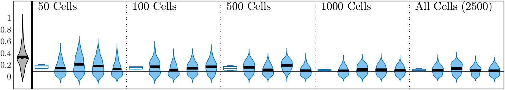
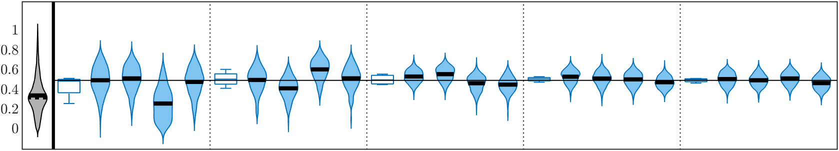
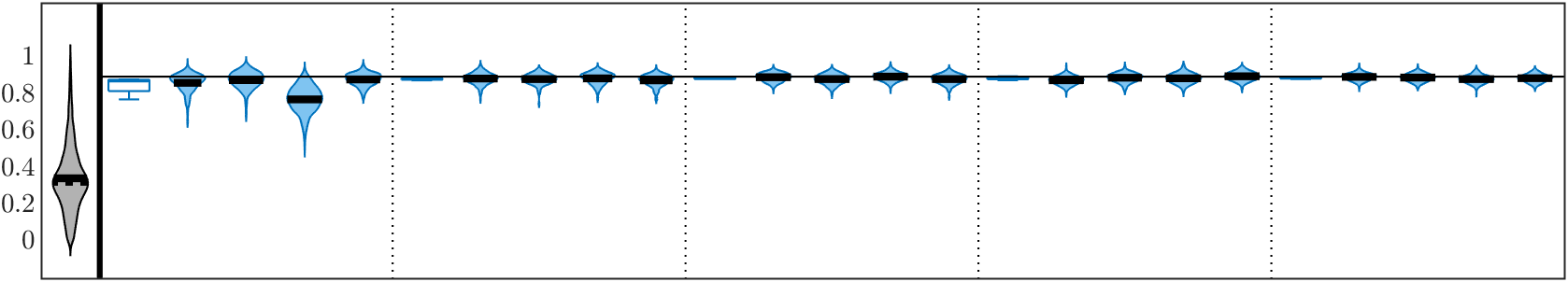
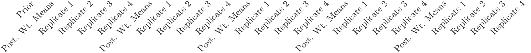
Figure 5: Prior density and posterior densities from individual replicates for $P_{\text{\tiny CC}}$ for different values of $S$, the number of cells sampled to calculate the approximation $\kappa_{S}(t)$ in fitting. Dashed and solid horizontal lines mark the weighted mean and median values respectively. For each value of $S$ we also show a boxplot of the distribution of posterior weighted means across all four replicates. We show results for the case where the target values of $\alpha$ and $\beta$ give rise to $P_{\text{\tiny CC}}$ values of approximately 0.1, 0.5, and 0.9 and $t_{\text{\tiny peak}}$ of approximately 18h. $\alpha$ and $\beta$ have units of $\text{h}^{-1}$ and $\text{(TCID}_{50}\text{/ml)}^{-1}\text{h}^{-1}$, respectively.

Discussion

In this work we have conducted a number of experiments to investigate the use of mathematical models in inferring the relative proportions of cell-to-cell and cell-free viral infection, which we summarised via the metric $P_{\text{\tiny CC}}$: the proportion of infections arising from the cell-to-cell route. We have applied simulation estimation techniques using Bayesian methods for inference on both an ODE model and a spatially-explicit multicellular model. As much as possible, we aimed to emulate the type and quality of data available experimentally.

In particular, we extracted and attempted to fit time series data on the proportion of fluorescent susceptible cells (that is, initially susceptible cells which have reached, or passed, the productively infected state), following experimental work Kongsomros and colleagues [13]. We found that this data source was insufficient for inferring $P_{\text{\tiny CC}}$ from simulation estimation after observational noise was applied, even when all model parameters aside from those governing the rates of cell-to-cell and cell-free infection were assumed known. This was true for both the ODE and spatial models. By contrast, from the same experiments, global metrics of the infection dynamics were very robustly inferred (the exponential growth rate $r$ for the ODE model, and the time of peak infected cell population $t_{\text{\tiny peak}}$ in the spatial case). This indicates that $P_{\text{\tiny CC}}$ values can be interchanged while preserving the fluorescent proportion curve — at least as precisely as can be estimated once observational noise is applied — provided $r$ or $t_{\text{\tiny peak}}$ are held fixed. This suggests that for both the ODE and spatial models, $P_{\text{\tiny CC}}$ cannot be inferred based on fluorescence data alone. The slight caveat to this claim was our observation that $P_{\text{\tiny CC}}$ was somewhat well estimated by the spatial model when the true proportion of cell-to-cell infections was high. This was due to the fact that in the spatial model, cell-to-cell infection is forced to spread radially, while cell-free infection is free to spread globally (causing the infected population to grow asymptotically exponentially). Therefore in instances where the global route of infection is almost entirely eliminated, the fluorescent population is forced to grow in a non-exponential manner, which was more easily detected by our inference methods.

We were able to overcome the inability to infer $P_{\text{\tiny CC}}$ by adding a second set of observational data alongside the fluorescent proportion time series. We did so by introducing a clustering metric $\kappa(t)$, which, given the state of the cell grid in a simulation of the spatial model, measures the mean fraction of fluorescent cells neighbouring each fluorescent cell. Note that since $\kappa(t)$ relies on knowledge of the actual spatial configuration of infection, it is only possible to construct such a metric for a spatially-structured model. We re-ran simulation estimations on the spatial model, using time series for both the fluorescent cell proportion and $\kappa(t)$ as the observational data, and found that $P_{\text{\tiny CC}}$ was very well estimated in this case regardless of the target value of $P_{\text{\tiny CC}}$, however estimates were especially precise when $P_{\text{\tiny CC}}$ was high.

We also found that $P_{\text{\tiny CC}}$ could still be reliably inferred using the spatial model when the clustering metric $\kappa(t)$ was only coarsely approximated, using a random subset of the cell population. Even at the coarsest approximation we tested — where $\kappa(t)$ was approximated using a sample of only 50 cells — inference of $P_{\text{\tiny CC}}$ was still reasonably robust, and dramatically improved compared to the case where $\kappa(t)$ was not used at all. These results suggest that even a very rough measure of the spatial distribution of infection is sufficient to deduce the $P_{\text{\tiny CC}}$ of the underlying system.

One of the limitations to the analysis which we have presented here is the fact that our simulation estimations have only attempted to fit the parameters governing the rates of infection (that is, $\alpha$ and $\beta$), and assumed perfect prior knowledge of all other model parameters. This prior knowledge is not available when fitting to actual experimental data. There are additional identifiability concerns attached with estimating the other parameters — the cell-free infection rate $\beta$ and extracellular viral production rate $p$, for instance, are well known to only be determined as a product [20, 11] — and it is possible that estimating these additional parameters may introduce further complications in determining $P_{\text{\tiny CC}}$. For the sake of simplicity, as well as computational complexity, we have not carried out this analysis in this work.

Another important simplification in our approach was our implementation of a global extracellular virus population in the spatial model, rather than a spatially-explicit, diffusing viral population. This approach, which was also employed by Blahut and colleagues in their dual-spread model of hepatitis C [2], implicitly assumes that extracellular viral transport over the cell grid is fast relative to the length scale of the cell sheet. This is fairly easily justified here due to the small grid of cells used in our implementation of the spatial model, but is also a standard assumption of the rate of viral diffusion in vivo or in permissive media [11, 8, 10, 15].

It is worth also briefly remarking on the computational costs associated with parameter estimation using these models. While the ODE model was very efficient to use, inference on the spatial model was extremely computationally intensive. The computation behind Figure 5, for instance, which comprises 60 individual simulation estimations took approximately 13 weeks to complete, with a single typical replicate taking around 24 hours each (running in parallel across eight CPUs (Intel Xeon CPU E5-2683 v4)), while our 150 ODE fits finished in ten days running on four CPUs (AMD EPYC 7702). This is despite using a small $50\times 50$ grid of cells for the spatial model and only fitting two parameters. The extremely high computational costs associated with these parameter estimations is largely due to the stochastic nature of the spatial model, meaning that many candidate parameter samples which are very close to the true values are randomly rejected. This effect is exacerbated when the noise associated with the model is increased, specifically, when the approximation of $\kappa(t)$ is especially coarse. While recent works in the literature have demonstrated rapid advancements in the speed of simulations by running on Graphic Processing Units [6] (our code, by contrast, is written in the comparatively slow MATLAB and run on CPUs), the computational costs associated with computing large-scale parameter estimations using the spatial model are not insignificant.

We opted to use fluorescence data as the main data source used in fitting, instead of extracellular viral titre data, which is more typically reported in the experimental virology literature. This is mainly because our work was guided by the results published by Kongsomros and colleagues [13], which reports fluorescent cell proportions as its main metric, but also since we were interested in analysing infection scenarios ranging from the extremes of purely cell-free to purely cell-to-cell, and cell fluorescence data is more relevant to predominantly cell-to-cell infections where cell-free virus has little influence on the dynamics. Furthermore, viral titre observations, as opposed to cell-based observations do not permit the collection of spatial information.

Our work is not the first in the literature to attempt to quantify the relative roles of cell-free and cell-to-cell infection routes. A number of mathematical modelling publications [15, 5, 2, 9], along with experimental works [27, 13] have applied varying models and methods to determine the prevalence of cell-to-cell infection. A common theme among the majority of these works [5, 2, 10, 27, 13] is the use of data collected from infections where one mode of infection is inhibited, usually by administering an antiviral drug such as oseltamivir for influenza [13], or by imposing a physical constraint on viral diffusion such as methylcellulose [27]. This approach is of limited relevance outside in vitro contexts and moreover relies on the extremely strong assumption that these interventions perfectly inhibit one infection mechanism while leaving the other unaltered.

The alternative approach — collecting data from experiments in which both modes of infection are unimpeded — raises additional challenges, but is more robust and, since it requires less invasive experimental intervention, dramatically widens the scope of experiments able to be used for inference. Kumberger and collaborators provided one early attempt at inferring the prevalence of cell-to-cell infection from this type of data. They used a spatial model with two modes of infection to generate synthetic global observational data (similar to the fluorescence data we have used here) and attempted to fit it using ODE models [15]. As we have found here, their work suggested that models which (artificially) account for the spatial structure of infection provided better estimates of the prevalence of cell-to-cell spread $P_{\text{\tiny CC}}$. However, even then, these estimates were still not especially accurate and were subject to systematic biases, even when fitting multiple observational datasets in a single fit. Our work provides context for these findings, offers novel insight on the identifiability of $P_{\text{\tiny CC}}$, and suggests an improved method for determining this quantity. We showed that ODE systems were unable to identify $P_{\text{\tiny CC}}$, even when fitting data generated by the system itself, and moreover showed that the collection of spatial information, in the form of the clustering metric $\kappa(t)$, was necessary to learn $P_{\text{\tiny CC}}$, even with a spatial model.

Our hope is that this work provides the foundations for applying mathematical modelling and inference methods to real experimental data in order to accurately quantify the relative roles of cell-free and cell-to-cell spread in real viral infections. The obvious extension to our work here is to apply our methods to experimental data. The data sources we have used here — the fluorescent cell proportion time series and the time series for the clustering metric $\kappa(t)$ — are readily obtainable (or at least estimable) from model cellular systems. This could be achieved in vitro by following methods similar to those described in Kongsomros et al. [13], and would only require simple staining and imaging techniques. After harvesting and fixing the cell sheet at one of a specified set of observation times, fluorescent cells are easily identified by staining with fluorescent antibodies and imaging the cell sheet. The resulting image could then be processed to compute the fluorescent proportion of the cell population, and to compute or estimate the clustering metric $\kappa(t)$. In brief, this work has explored the identifiability of the relative proportions of cell-free and cell-to-cell infection (the latter of these we termed $P_{\text{\tiny CC}}$) in two standard models of dual-spread viral dynamics: one ODE model and one spatially-explicit multicellular model. We showed that $P_{\text{\tiny CC}}$ could not be determined using either model when only the proportion of fluorescent cells was reported. We found that when an additional data source, describing the clustering structure of the infection, was also used for fitting, $P_{\text{\tiny CC}}$ could be accurately determined using the spatial model. This was the case even when the clustering metric was only approximated using a small sample of the cell sheet. Our results imply that some degree of information about the spatial structure of infection is necessary to infer $P_{\text{\tiny CC}}$. We have demonstrated practically obtainable data types which, combined with experimental collaboration, could lead to more precise and robust predictions of the role of the two modes of viral spread.

Methods

An ODE model for dual-spread dynamics

We employ an ODE model which is adapted from a typical model of viral dynamics with two modes of spread [15], which is in turn based on the standard model of viral dynamics [20]. We make the additional inclusion of a latent phase of infection, based on observations from data published by Kongsomros and colleagues [13]. We noticed a delay in the initial uptick of the fluorescent cell time series curve, indicating that cells only become detectably fluorescent once they are productively infected, that is, following the eclipse phase of infection. We tested having both single and multiple latent stages in the model — or equivalently, exponentially and gamma-distributed durations for the eclipse phase — and obtained dramatically improved agreement with the data when we assumed multiple latent stages before cells become detectably fluorescent. This approach is common in representing the eclipse phase of infection in the literature [21, 6]. We arrived at the following form of the model, in ODE form:

$$\frac{dT}{dt} =-\alpha TI-\beta TV,$$ (1)

$$\frac{dE^{(1)}}{dt} =\alpha TI+\beta TV-K\gamma E^{(1)},$$ (2)

$$\frac{dE^{(k)}}{dt} =K\gamma\left(E^{(k-1)}-E^{(k)}\right),\qquad\text{for }k=2,3,...,K,$$ (3)

$$\frac{dI}{dt} =K\gamma E^{(K)}-\delta I,$$ (4)

$$\frac{dV}{dt} =pI-cV,$$ (5)

where $T$ is the fraction of cells susceptible to infection, $\sum_{i=1}^{K}E^{(i)}$ is the fraction of cells in the eclipse phase of infection, $I$ is the fraction of cells in the productively infected state, and $V$ is the quantity of extracellular virus. Since we wish to keep track of whether infections come from the cell-to-cell or cell-free infection routes, we incorporate the following subsystem which keeps track of the cumulative proportion of the target population which has become infected via the cell-to-cell mechanism ($F_{\text{\tiny CC}}$) or the cell-free mechanism ($F_{\text{\tiny CF}}$). We have

$$\frac{dE_{\text{\tiny CC}}^{(1)}}{dt} =\alpha TI-K\gamma E_{\text{\tiny CC}}^{(1)},$$ (6)

$$\frac{dE_{\text{\tiny CC}}^{(k)}}{dt} =K\gamma\left(E_{\text{\tiny CC}}^{(k-1)}-E_{\text{\tiny CC}}^{(k)}\right),\qquad\text{for }k=2,3,...,K,$$ (7)

$$\frac{dE_{\text{\tiny CF}}^{(1)}}{dt} =\beta TV-K\gamma E_{\text{\tiny CF}}^{(1)},$$ (8)

$$\frac{dE_{\text{\tiny CF}}^{(k)}}{dt} =K\gamma\left(E_{\text{\tiny CF}}^{(k-1)}-E_{\text{\tiny CF}}^{(k)}\right),\qquad\text{for }k=2,3,...,K,$$ (9)

$$\frac{dF_{\text{\tiny CC}}}{dt} =\frac{K\gamma}{T_{0}}E_{\text{\tiny CC}}^{(K)},$$ (10)

$$\frac{dF_{\text{\tiny CF}}}{dt} =\frac{K\gamma}{T_{0}}E_{\text{\tiny CF}}^{(K)},$$ (11)

where $T_{0}=T(0)$ is the initial target cell proportion. The sum of these two quantities,

$$F(t)=F_{\text{\tiny CC}}(t)+F_{\text{\tiny CF}}(t),$$ (12)

is the cumulative proportion of the cell population which has become infected through either mechanism, which we take to be equivalent to the proportion of fluorescent cells as observed in Kongsomros et al. [13]. The assumption that cells remain fluorescent even after they die (over the time scale of interest) is justified by the observation that in Kongsomros et al. fluorescent proportions were observed to saturate at 100% at later times in their experiments

Throughout this work, we will assume fixed values of the parameters $K$, $\gamma$, $\delta$, $p$, and $c$, as specified in Table 1. These parameters were obtained by running a Bayesian parameter estimation for the form of the ODE model as defined above against fluorescent cell time series data in [13], and selecting one particular posterior sample at random (results not shown for sake of brevity). These values were selected simply to be indicative of the realistic range of values for these parameters and are sufficiently realistic for the purposes of this work. In each case we initiate the infection by setting $T(0)=0.99$, $I(0)=0.01$ and the remaining compartments to zero.

Description	Symbol	Value and Units
Number of delay compartments	K	3
Eclipse cell activation rate	$\gamma$	$3.366934\times 10^{-1}\text{h}^{-1}$
Death rate of infected cells	$\delta$	$8.256588\times 10^{-2}\text{ h}^{-1}$
Extracellular virion production rate	$p$	$1.321886\times 10^{6}(\text{ TCID}_{50}\text{/ml})\text{ h}^{-1}$
Extracellular virion clearance rate	$c$	$4.313531\times 10^{-1}\text{ h}^{-1}$

Table 1: Fixed parameters used in our simulations.

A multicellular spatial model for dual-spread dynamics

It is straightforward to adapt this system of ODEs into a spatially-structured multicellular model, that is, a model which tracks the dynamics of a finite number of discrete cells which each occupy some specified region of space and at any given point in time, may be in one of a set of cell states [22, 26]. Suppose we model the dynamics of a population of $N$ cells. We associate with each of these cells an index $i\in\left\{1,2,...,N\right\}$, and a cell state at time $t$ given by $\sigma_{i}(t)$, where the possible cell states correspond to the compartments of the ODE system, including the implicit dead cell compartment. That is, for any cell $i$, $\sigma_{i}(t)\in\left\{T,E,I,D\right\}$, representing the target, eclipse, infected and dead state respectively.

For the spatial model, following Blahut and colleagues [2], we make the simplifying assumption that the dispersal of free virions over the computational domain is fast, and that the extracellular viral distribution can therefore be considered approximately uniform. As such, the equation for $V$ in our spatial model changes only in notation from Equation (5):

$$\frac{dV}{dt}=p\sum_{i=1}^{N}\frac{\mathbbm{1}_{\left\{\sigma_{i}(t)=I\right\}}}{N}-cV.$$ (13)

As such, cell-free infection is considered a spatially global mode of spread in our spatial model. By contrast, following results from the biological literature, we assume that cell-to-cell spread is a spatially local mechanism [14, 13]. As such, we assume that the probability of cell-to-cell infection in the spatial model depends not on the global proportion of infected cells as in Equation (1), but rather the proportion of a cell’s neighbours which are infected. Specifically, if we denote by $\nu(i)$ the set of indices of the cells neighbouring cell $i$, the probability of cell $i$ becoming infected by cell-to-cell infection over a given time period depends on the term $\sum_{j\in\nu(i)}(\mathbbm{1}_{\left\{\sigma(j)=I\right\}})/\left|\nu(i)\right|$.

Combining these two mechanisms, we obtain the following transition probability for target cell $i$ to become (latently) infected over some time interval $\Delta t$:

$$P(\sigma_{i}(t+\Delta t)=E|\sigma_{i}(t)=T)=1-\exp\left(-\left(\alpha\sum_{j\in\nu(i)}\frac{\mathbbm{1}_{\left\{\sigma_{j}(t)=I\right\}}}{\left|\nu(i)\right|}+\beta V\right)\Delta t\right)$$ (14)

For the eclipse phase, instead of implementing transition probabilities for each $E^{(k)}$, for computational simplicity we instead sample a latent phase duration from its probability distribution at the time a cell first enters the eclipse state. That is, if we write $t_{i}^{E}=\min\{t:\sigma_{i}(t)=E\}$ for the time at which cell $i$ enters the eclipse state, and $t_{i}^{I}=\min\{t:\sigma_{i}(t)=I\}$ for the time at which cell $i$ enters the productively infected state, we have

$$t_{i}^{I}=t_{i}^{E}+\tau_{i},$$ (15)

where

$$\tau_{i}\sim\text{\emph{Gamma}}\left(K,\frac{1}{K\gamma}\right).$$ (16)

The remaining compartments are easily described by simple transition probabilities.

$$P(\sigma_{i}(t+\Delta t)=I|\sigma_{i}(t)=E)=1-\exp\left(-K\gamma\Delta t\right),$$ (17)

$$P(\sigma_{i}(t+\Delta t)=D|\sigma_{i}(t)=I)=1-\exp\left(-\delta\Delta t\right).$$ (18)

Equations (13)–(18), together with appropriate initial and boundary conditions, define the spatial model. Note that the spatial structure of this model is not explicit, but rather is defined by the adjacency function $\nu(\cdot)$. Nonetheless, we will take the spatial configuration of our model tissue to be as follows. We consider a two-dimensional sheet of cells with hexagonal packing of cells and periodic boundary conditions in both the $x$ and $y$ directions, such that each cell has precisely size neighbours. This packing reflects the arrangement of cells in real epithelial monolayers and has the practical benefit that all adjacent cells are joined via a shared edge, avoiding any complications associated with corner-neighbours. Throughout this work we use a $50\times 50$ grid of cells, and, following equivalent initial conditions as for the ODE model, we initiate infection by randomly selecting 1% of the cell sheet to be initially infected, and the remainder of the sheet to be susceptible to infection. In Figure 3(a) we show a schematic of the model as well as the layout of the cell grid. This is not a novel model. This model structure, or slight variations thereof, has been used in a number of recent publications describing infection dynamics with two modes of viral spread and has become somewhat of a standard approach in the field in recent years [9, 2, 5, 6].

As with the ODE model, we can additionally keep track of the cumulative proportion of infections arising from each mode of infection individually in the spatial model. As addition to the overall probability of infection in Equation (14), we can compute a probability of infection by each mode of spread individually as follows. Using the same Poisson process argument as above, the probability of cell-to-cell infection of cell $i$ not taking place over the time interval $\left[t,t+\Delta t\right]$ is given by

$$P(\mathbf{E}_{i}^{\text{\tiny CC}}\notin\left[t,t+\Delta t\right])=\exp\left(-\alpha\sum_{j\in\nu(i)}\frac{\mathbbm{1}_{\left\{\sigma_{j}(t)=I\right\}}}{\left|\nu(i)\right|}\Delta t\right),$$ (19)

and the probability of cell-free infection of cell $i$ not occurring over the same time interval is given by

$$P(\mathbf{E}_{i}^{\text{\tiny CF}}\notin\left[t,t+\Delta t\right])=\exp\left(-\beta V\Delta t\right),$$ (20)

where $\mathbf{E}_{i}^{CC}$ and $\mathbf{E}_{i}^{CF}$ are the events of a cell-to-cell infection and a cell-free infection occurring at cell $i$ respectively. Note that we have to account for the fact that while, mathematically, both events may occur in the time interval $\left[t,t+\Delta t\right]$, we need to assign a unique mode of transmission to each infection. We do so as follows. The following calculation is also derived in work by Blahut and colleagues [2]. If we write $m(i)\in\left\{CC,CF\right\}$ for the mode of infection of cell $i$, then at the time of infection of cell $i$ — that is, when $t=t_{i}^{E}$ — we compute the probability of each individual mode of transmission as follows:

$$P(m(i)=CC)=\frac{1-P(\mathbf{E}_{i}^{\text{\tiny CC}}\notin\left[t,t+\Delta t\right])}{2-P(\mathbf{E}_{i}^{\text{\tiny CC}}\notin\left[t,t+\Delta t\right])-P(\mathbf{E}_{i}^{\text{\tiny CF}}\notin\left[t,t+\Delta t\right])}$$ (21)

and

$$P(m(i)=CF)=\frac{1-P(\mathbf{E}_{i}^{\text{\tiny CF}}\notin\left[t,t+\Delta t\right])}{2-P(\mathbf{E}_{i}^{\text{\tiny CC}}\notin\left[t,t+\Delta t\right])-P(\mathbf{E}_{i}^{\text{\tiny CF}}\notin\left[t,t+\Delta t\right])}$$ (22)

In our model, therefore, when an infection is detected, we draw a random number $p\sim\text{\emph{Uniform}}(0,1)$, and if $p<P(m(i)=CC)$, we designate the infection a cell-to-cell infection, otherwise, it is considered a cell-free infection. We use a similar calculation to assign the viral lineage associated with an infection, which we used to construct the colouring of cells in Figure 3(d), which we stipulate in full in Supplementary Section 2. The quantities $F_{\text{\tiny CC}}$ and $F_{\text{\tiny CF}}$ can easily be calculated for the spatial model as

$$F_{\text{\tiny CC}}(t)=\frac{\sum_{i=1}^{N}\mathbbm{1}_{\left\{m(i)=CC\right\}}\mathbbm{1}_{\left\{t_{i}^{I}\in\left[0,t\right]\right\}}\mathbbm{1}_{\left\{\sigma_{i}(0)=T\right\}}}{\sum_{i=1}^{N}\mathbbm{1}_{\left\{\sigma_{i}(0)=T\right\}}},$$ (23)

$$F_{\text{\tiny CF}}(t)=\frac{\sum_{i=1}^{N}\mathbbm{1}_{\left\{m(i)=CF\right\}}\mathbbm{1}_{\left\{t_{i}^{I}\in\left[0,t\right]\right\}}\mathbbm{1}_{\left\{\sigma_{i}(0)=T\right\}}}{\sum_{i=1}^{N}\mathbbm{1}_{\left\{\sigma_{i}(0)=T\right\}}},$$ (24)

which allow us to keep track of the count of each type of infection event throughout simulations of the spatial model. As before, we define

$$F(t)=F_{\text{\tiny CC}}(t)+F_{\text{\tiny CF}}(t).$$ (25)

Metrics

Proportion of infections from the cell-to-cell route – $P_{\text{\tiny CC}}$

We introduce the quantity $P_{\text{\tiny CC}}$ to denote the proportion of infections arising from the cell-to-cell route. This is calculated by keeping track of the cumulative proportion of the target cell population which becomes infected by either infection mechanism over time. At long time — once the infection has essentially run its course — we compute $P_{\text{\tiny CC}}$ as the fraction of the total infections which occurred via cell-to-cell infection. Using $F_{\text{\tiny CC}}$ and $F_{\text{\tiny CF}}$ as we have defined them, we have

$$P_{\text{\tiny CC}}=\lim_{t\rightarrow\infty}\frac{F_{\text{\tiny CC}}(t)}{F_{\text{\tiny CC}}(t)+F_{\text{\tiny CF}}(t)}.$$ (26)

In Figure 1(c) we show an illustration of this calculation more generally.

$P_{\text{\tiny CC}}$ quantifies the relative weight of the cell-to-cell route of infection and is therefore our target for estimation in this work. Its definition is general and is not specific to any particular model structure. $P_{\text{\tiny CC}}$ cannot be directly calculated in closed form directly from the model parameters. Instead, we repeatedly simulate our model using parameters sampled from $\alpha$–$\beta$ space and compute $P_{\text{\tiny CC}}$ in order to construct lookup tables. In Figure 1(d), we plot a contour map of $P_{\text{\tiny CC}}$ values for the ODE model in $\alpha$–$\beta$ space. In the case of the spatial model, we accounted for the inherent stochasticity of the model by running 20 simulations of the model at each $(\alpha,\beta)$ pair in the lookup table and kept track of mean $P_{\text{\tiny CC}}$ values. The associated contour map for the spatial model is shown in Figure 6(a). Contour plots were generated by computing contours over the lookup table using MATLAB’s contourf function. We interpolate between values on the lookup table by constructing spline fits along $\alpha$ and $\beta$ contours.

Exponential growth rate – $r$

A second quantity, which describes the overall rate of infection spread is the exponential growth rate $r$. This quantity, related to the basic reproduction number $\mathcal{R}_{0}$, is well-established in the theory of epidemiological and virus dynamical models and has the property that, for small $t$, we have $I(t)\approx I_{0}e^{rt}$ [3, 17, 18, 4]. The exponential growth rate for the ODE model can be readily computed by linearising the ODE system about the infection free steady state and finding the dominant eigenvalue of the resulting system [17, 4]. For our model, we obtain the following explicit definition:

$$r=\max{\left\{\lambda~{}:~{}g(\lambda)=0\right\}},$$ (27)

where

$$g(\lambda):=\left(1+\frac{\lambda}{K\gamma}\right)^{K}\left(c+\lambda\right)\left(\delta+\lambda\right)-\left(\alpha\left(c+\lambda\right)+\beta p\right).$$

Time to peak infected cell population – $t_{\text{\tiny peak}}$

The exponential growth rate $r$ relies on asymptotically exponential behaviour of the infected proportion curve. However, for the spatial model, especially in instances where infections spread mainly locally — that is, through the cell-to-cell route — the infected proportion curve does not grow exponentially. For the spatial model, therefore, $r$ is not well-defined. We instead use the time of the peak infected cell proportion, which we label as $t_{\text{\tiny peak}}$, as an alternative measure of the overall growth behaviour of the infected population. As with $P_{\text{\tiny CC}}$, this quantity is not easily approximated a priori, therefore we also compute lookup tables in $\alpha$–$\beta$ space for this quantity. We show the contour map of $t_{\text{\tiny peak}}$ on $\alpha$–$\beta$ space in Figure 6(b). Contour plots were generated by computing contours over the lookup table using MATLAB’s contourf function.

It is worth mentioning that the time of the peak infected cell population is a quantity that is not typically experimentally observable, whereas a quantity like the time of peak viral load is comparatively much easier to measure in an experimental context. However, we opt to use the latter metric, since this is a meaningful metric of the model regardless of the mechanism of infection spread. Even in a scenario where all infections in the model arise from the cell-to-cell route (i.e. $P_{cc}=1$) the time of peak infected population remains a relevant as a measure of the overall rate of infection progression, where the time of the peak extracellular viral load is far less meaningful here. In any event, for our purposes in this work, $t_{\text{\tiny peak}}$ is used simply to illustrate a quantity which represents the overall rate of infection spread in a model simulation, and a quantity which we observe to be preserved between accepted samples of our simulation estimation (at least when clustering data are not used). This choice of metric does not diminish the relevance of our analysis to experimental application.

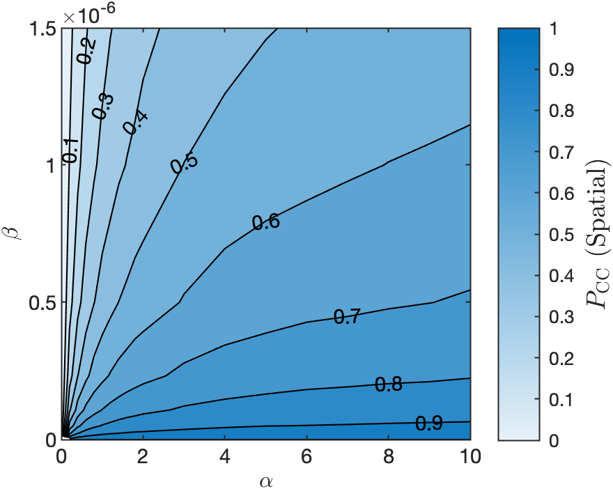
(a)

(b)

Figure 6: $P_{\text{\tiny CC}}$ and $t_{\text{\tiny peak}}$ contour maps respectively on $\alpha$–$\beta$ space for the spatial model. $\alpha$ and $\beta$ have units of $\text{h}^{-1}$ and $\text{(TCID}_{50}\text{/ml)}^{-1}\text{h}^{-1}$, respectively.

0.0.1 Clustering metric – $\kappa(t)$ (and approximation – $\kappa_{S}(t)$)

Given a cell grid where we denote by $\mathcal{F}(t)$ the set of cells which are fluorescent, we compute for each fluorescent cell $i\in\mathcal{F}(t)$ the quantity $k_{i}(t)$, which is the proportion of the neighbours of cell $i$ which are also fluorescent. We then define $\kappa(t)$ as the mean of the $k_{i}(t)$s. We compute $\kappa(t)$ over time $t$ to form a time series. In Figures 3(a) and 3(g), we show an example of computing fluorescent neighbour proportions, and plot example $\kappa(t)$ time series for three parameter pairs, corresponding to $P_{\text{\tiny CC}}$ values of 0.1, 0.5, and 0.9. Figure 3(g), shows that, unlike with the fluorescent cell time series, there is substantial variation in the $\kappa(t)$ curves with changing $P_{\text{\tiny CC}}$.

$\kappa(t)$ has the property that when it is near zero, fluorescent cells are mostly isolated and the infection is very diffuse, and when it is near one, fluorescent cells are generally found in clusters, indicating that the infection is very compact. In principle, $\kappa(t)$ could be computed or estimated in experimental settings with the use of fluorescence imaging of the cell sheet, samples of which can be found in works by Kongsomros et al. and Fukuyama et al. [13, 7].

We modify the definition of $\kappa(t)$ to define the approximation $\kappa_{S}(t)$ as follows. Given a grid of $N$ cells at time $t$, of which the fluorescent population is given by $\mathcal{F}(t)$ as before, we draw $S\leq N$ cells without replacement and call the set of sampled cells $\mathcal{S}(t)$. For each sampled cell $i$, if $i\in\mathcal{F}(t)$, we compute $k_{i}(t)$, and then compute the approximate clustering metric $\kappa_{S}(t)$ as the mean of the computed $k_{i}(t)$s, that is, if $\left|\mathcal{S}(t)\cap\mathcal{F}(t)\right|\neq 0$, then

$$\kappa_{S}(t)=\sum_{i\in\mathcal{S}(t)\cap\mathcal{F}(t)}\frac{k_{i}(t)}{\left|\mathcal{S}(t)\cap\mathcal{F}(t)\right|}.$$

In the event that no fluorescent cells are sampled (that is, $\left|\mathcal{S}(t)\cap\mathcal{F}(t)\right|=0$), we define $\kappa_{S}(t)=0$.

Simulation estimation

Throughout this work we conduct a series of simulation estimation experiments to explore what can be learned about the roles of the two modes of viral spread based on observed model outputs. We outline here the general framework of this process.

For both the ODE and the spatial model, we begin by drawing a set of target values for the infection parameters $\alpha$ and $\beta$. As mentioned above, the values of the other model parameters are considered fixed and known. We then simulate the chosen model using these parameter values, and apply an observational model $f(\cdot)$ to its output to generate a set of observed data $\mathbf{D}$. The observational model $f$ is designed to simulate the noise incurred in actual experiments. Throughout this work, we focus especially on the observed fluorescent cell proportion over time, since this is the main source of data reported by Kongsomros and colleagues [13].

For the ODE model, we obtain the observed fluorescent cell proportion $\mathbf{D}$ by computing the true fluorescent cell time series $F(t)$ (defined in Equation (12)) at each of a series of observation times, converting this proportion to a count of fluorescent cells and applying negative binomial noise. The negative binomial distribution reflects the observed error structure in [13], which is constructed from overdispersed count data. We assume some vector of observation times $\mathbf{t}=\left\{t_{1},t_{2},...t_{m}\right\}$ and define

$$\mathbf{D}_{\text{\tiny ODE}}=f_{\text{\tiny ODE}}(F(t);\mathbf{t},k,N_{\text{\tiny sample}})=\left(\frac{1}{N_{\text{\tiny sample}}}\right)\cdot\left\{D_{1},D_{2},...,D_{m}\right\},$$ (28)

where

$$D_{i}\sim\text{\emph{Negative Binomial}}\left(N_{\text{\tiny sample}}F(t_{i}),\phi\right)$$

for $i=1,2,...,m$, where $N_{\text{\tiny sample}}F(t_{i})$ and $\phi$ are the mean and dispersion parameter respectively of $D_{i}$. $N_{\text{\tiny sample}}$ is the number of cells measured for fluorescence, in a sense the size of the cell population. $\text{Var}\left[D_{i}\right]=N_{\text{\tiny sample}}F(t_{i})+\left[N_{\text{\tiny sample}}F(t_{i})\right]^{2}/\phi$ for all $i=1,2,...m$. In Figure 7(b), we show an illustration of this observation process. The curve shown in blue is the true fluorescent proportion curve $F(t)$. At each of the observation times, indicated with dots, we apply noise about the true value.

After obtaining observed data $\mathbf{D}_{\text{\tiny ODE}}$, we then re-estimate $\alpha$ and $\beta$ using Bayesian methods. We assume uniform prior distributions

$$\pi_{\alpha}(\alpha)=\begin{cases}1/\alpha_{\text{\tiny max}},~{}\alpha\in[0,\alpha_{\text{\tiny max}}]\\ 0,~{}\text{otherwise}\end{cases},$$ (29)

$$\pi_{\beta}(\beta)=\begin{cases}1/\beta_{\text{\tiny max}},~{}\beta\in[0,\beta_{\text{\tiny max}}]\\ 0,~{}\text{otherwise}\end{cases},$$ (30)

with $\alpha_{\text{ \tiny max}}=2.5\text{h}^{-1}$, $\beta_{\text{\tiny max}}=2\times 10^{-6}\text{(TCID}_{50}\text{/ml)}^{-1}\text{h}^{-1}$. We re-estimate $\alpha$ and $\beta$ using No U-Turn Sampling (NUTS) Markov Chain Monte Carlo (MCMC) methods with a negative binomial likelihood

$$D_{i}\sim\text{\emph{Negative Binomial}}\left(N_{\text{\tiny sample}}\hat{F}(t_{i}),\phi\right)$$ (31)

for $i=1,2,...,m$, where $\hat{F}(t)$ is the fluorescent proportion time series estimated by simulating the ODE model using samples $\hat{\alpha}$ and $\hat{\beta}$. For each estimation we use four chains seeded with random initial values and draw 2000 samples for each, including 200 burn-in samples. We assume $N_{\text{ \tiny sample}}=200,000$, which was the number of cells used in the experiments in [13].

For the spatial model, we have two sources of observational data: both the fluorescent proportion time series and the clustering metric $\kappa(t)$. Since the system is inherently stochastic, we do not add additional external noise, instead, we aim to emulate the experimental process whereby the fluorescent proportion of a cell population (and consequently the clustering metric) cannot be observed without destroying, or at least disrupting, the cell sheet. We implement this by sampling our observations from $m$ independent simulations of the model. That is, if we have observation times $\mathbf{t}=\left\{t_{1},t_{2},...,t_{m}\right\}$ and $m$ true fluorescence and clustering time series from independent simulations of the spatial model, $\mathbf{F}(t)=\left\{F_{1}(t_{1}),F_{2}{t_{2}},...,F_{m}(t_{m})\right\}$ and $\mathbf{K}(t)=\left\{\kappa_{1}(t_{1}),\kappa_{2}(t_{2}),...,\kappa_{m}{t_{m}}\right\}$ respectively, we generate the two sets of observational data

$$\mathbf{D}_{\text{\tiny spatial}}^{\text{\tiny fluoro}}=f_{\text{\tiny spatial}}(\mathbf{F}(t);\mathbf{t})=\left\{F_{1}(t_{1}),F_{2}(t_{2}),...F_{m}(t_{m})\right\},$$ (32)

$$\mathbf{D}_{\text{\tiny spatial}}^{\text{\tiny cluster}}=f_{\text{\tiny spatial}}(\mathbf{K}(t);\mathbf{t})=\left\{\kappa_{1}(t_{1}),\kappa_{2}(t_{2}),...\kappa_{m}(t_{m})\right\}.$$ (33)

We show a demonstration of this observation process in Figure 7(c).

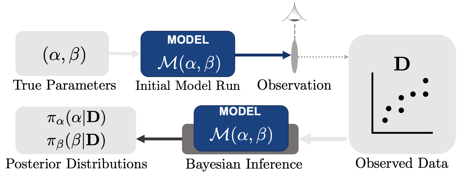
(a)

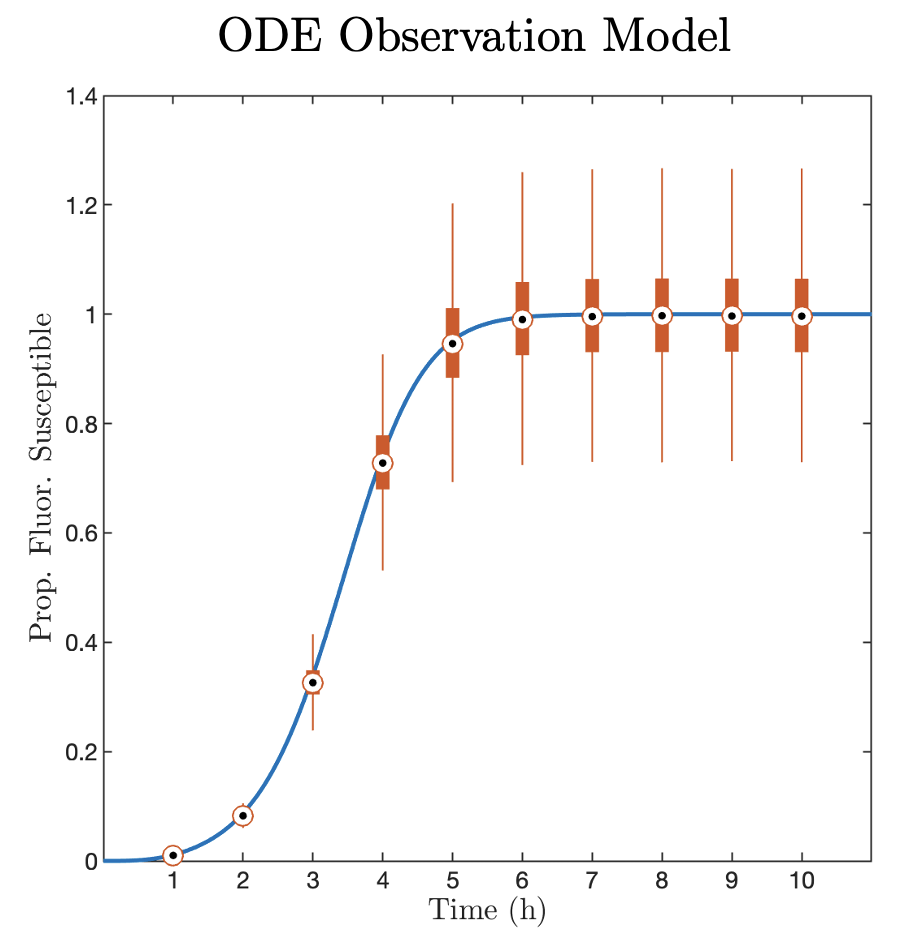
(b)

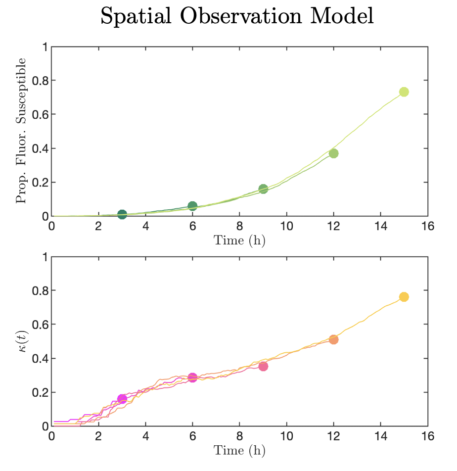
(c)

Figure 7: (a) Schematic of the simulation estimation process. (b)–(c) Observation model for fluorescent proportion of susceptible cells for (b) the ODE model and (c) the spatial model (first five points shown). In the spatial case we also show the observation model for the clustering metric $\kappa(t)$. For the ODE model, we sample the true fluorescent proportion curve at a series of time points (shown in blue), then observe a value based on a negative binomial distribution centred on the true value (box plot of the distribution shown in orange). Here, $\phi=10^{2}$. For the spatial model, we run independent iterations of the stochastic model and observe one point from each.

Due to the stochasticity of the system, we use Approximate Bayesian Computation (ABC) to re-estimate $\alpha$ and $\beta$ for the spatial model. In particular, we adapt the Population Monte Carlo (PMC) method introduced by Toni and collaborators [25] and revised by others [1, 16]. We sketch this method in pseudocode in Algorithm 1.

Algorithm 1 PMC algorithm for parameter estimation using the spatial model - fluorescence and clustering data

Input: Model $\mathcal{M}(\alpha,\beta)$, prior distributions for target parameters $\pi_{\alpha}(\alpha)$ and $\pi_{\beta}(\beta)$, target number of particles $N_{P}$, number of generations $G$, reference data $\mathbf{D}^{\text{ \tiny fluoro}}$ and $\mathbf{D}^{\text{ \tiny cluster}}$ , distance metrics $d^{\text{\tiny fluoro}}(\cdot,\cdot)$ and $d^{\text{\tiny cluster}}(\cdot,\cdot)$, perturbation kernel $K(\cdot|\cdot)$, initial acceptance proportion $p_{\text{\tiny 0,accept}}$, threshold tightening parameter $q$.

Output: Weighted samples from the posterior distributions $\hat{\pi}_{\alpha}(\alpha|\mathbf{D}^{\text{ \tiny fluoro}},\mathbf{D}^{\text{ \tiny cluster}})$, $\hat{\pi}_{\beta}(\beta|\mathbf{D}^{\text{ \tiny fluoro}},\mathbf{D}^{\text{ \tiny cluster}})$.

Rejection sampling

for $i=1,2,...,\left\lceil N_{P}/p_{\text{\tiny 0,accept}}\right\rceil$  do

     Randomly draw $\hat{\alpha}_{i}$ and $\hat{\beta}_{i}$ from $\pi_{\alpha}(\alpha)$ and $\pi_{\beta}(\beta)$, respectively.

     Obtain the model output using these parameters, $\left\{\hat{\mathbf{D}}_{i}^{\text{\tiny fluoro}},\hat{\mathbf{D}}_{i}^{\text{\tiny cluster}}\right\}=\mathcal{M}(\hat{\alpha}_{i},\hat{\beta}_{i})$.

      Compute the distance between model output and reference data $\epsilon_{i}^{\text{\tiny fluoro}}=d^{\text{\tiny fluoro}}(\hat{\mathbf{D}}_{i}^{\text{\tiny fluoro}},\hat{\mathbf{D}}^{\text{\tiny fluoro}})$ and $\epsilon_{i}^{\text{\tiny cluster}}=d^{\text{\tiny cluster}}(\hat{\mathbf{D}}_{i}^{\text{\tiny cluster}},\hat{\mathbf{D}}^{\text{\tiny cluster}})$ .

end for

$n_{\text{\tiny opt found}}\leftarrow 0$, $T\leftarrow 0$

while $n_{\text{\tiny opt found}}<N_{P}$ do

     $T\leftarrow T+1$, define $\mathcal{I}_{1},\mathcal{I}_{2},...,\mathcal{I}_{n_{\text{\tiny opt found}}},$ as the indices $i$ in the smallest $T$ values of the $\epsilon_{i}^{\text{\tiny fluoro}}$s and the smallest $T$ values of the $\epsilon_{i}^{\text{\tiny fluoro}}$s.

end while

for $j=1,2,...,N_{P}$ do

     Set $\mathcal{P}_{j}=(\hat{\alpha}_{\mathcal{I}_{j}},\hat{\beta}_{\mathcal{I}_{j}})$.

     Set $w_{j}=1/N_{P}$.

end for

$\mathcal{P}=\left\{\mathcal{P}_{1},\mathcal{P}_{2},...,\mathcal{P}_{N_{P}}\right\}$ is the initial particle population. $w=\left\{w_{1},w_{2},...,w_{N_{P}}\right\}$ is the initial weight vector. Set the distance thresholds $\epsilon_{D}^{\text{\tiny fluoro}}$ and $\epsilon_{D}^{\text{\tiny cluster}}$ as the $q^{th}$ quantile of the $\epsilon_{i}^{\text{\tiny fluoro}}$s and $\epsilon_{i}^{\text{\tiny cluster}}$s respectively.

Importance sampling

for $g=1,2,...,G$ do

     Set number of accepted particles $N_{\text{\tiny accepted}}\leftarrow 0$

     while $N_{\text{\tiny accepted}}<N_{P}$ do

         Randomly draw a particle $\mathcal{P}_{j}$ with probability $w_{j}$.

         Perturb particle by the kernel $K(\cdot|\mathcal{P}_{j})$ to obtain a new sample $(\hat{\alpha},\hat{\beta})$.

         Obtain the model output using these parameters, $\left\{\hat{\mathbf{D}}_{i}^{\text{\tiny fluoro}},\hat{\mathbf{D}}_{i}^{\text{\tiny cluster}}\right\}=\mathcal{M}(\hat{\alpha}_{i},\hat{\beta}_{i})$.

          Compute the distance between model output and reference data $\epsilon_{i}^{\text{\tiny fluoro}}=d^{\text{\tiny fluoro}}(\hat{\mathbf{D}}_{i}^{\text{\tiny fluoro}},\hat{\mathbf{D}}^{\text{\tiny fluoro}})$ and $\epsilon_{i}^{\text{\tiny cluster}}=d^{\text{\tiny cluster}}(\hat{\mathbf{D}}_{i}^{\text{\tiny cluster}},\hat{\mathbf{D}}^{\text{\tiny cluster}})$ .

         if $\epsilon_{i}^{\text{\tiny fluoro}}<\epsilon_{D}^{\text{\tiny fluoro}}$ and $\epsilon_{i}^{\text{\tiny cluster}}<\epsilon_{D}^{\text{\tiny cluster}}$ then

              Set $N_{\text{\tiny accepted}}\leftarrow N_{\text{\tiny accepted}}+1$ and $\mathcal{P}_{N_{\text{\tiny accepted}}}^{\text{\tiny next}}=(\hat{\alpha}_{i},\hat{\beta}_{i})$.

         else

              Return to start of while.

         end if

     end while

     for $i=1,2,...,N_{P}$ do

         Set $w_{i}^{*,\text{\tiny next}}=w_{i}/\sum_{j=1}^{N_{P}}K\left(\mathcal{P}_{i}^{\text{\tiny next}}|\mathcal{P}_{j}\right)w_{j}$

     end for

     Set $\mathcal{P}\leftarrow\left\{\mathcal{P}_{1}^{\text{\tiny next}},\mathcal{P}_{2}^{\text{\tiny next}},...,\mathcal{P}_{N_{P}}^{\text{\tiny next}}\right\}$, $w\leftarrow(1/\sum_{i=1}^{N_{P}}w_{i}^{*,\text{\tiny next}})\cdot\left\{w_{1}^{*,\text{\tiny next}},w_{2}^{*,\text{\tiny next}},...,w_{N_{P}}^{*,\text{\tiny next}}\right\}$

     Set the distance thresholds $\epsilon_{D}^{\text{\tiny fluoro}}$ and $\epsilon_{D}^{\text{\tiny cluster}}$ as the $q^{th}$ quantile of the $\epsilon_{i}^{\text{\tiny fluoro}}$s and $\epsilon_{i}^{\text{\tiny cluster}}$s respectively.

end for

In our case, the model $\mathcal{M}(\hat{\alpha},\hat{\beta})$ is simply the time series $F(t)$ obtained by a single simulation of the spatial model with parameters $\alpha=\hat{\alpha}$ and $\beta=\hat{\beta}$, and evaluated at time points $\mathbf{t}$, the vector of time points at which the reference data $\mathbf{D}$ is obtained. We again use the uniform prior distributions in Equations (29) and (30), although now with $\alpha_{max}=10\text{h}^{-1}$, $\beta_{max}=1.5\times 10^{-6}\text{(TCID}_{50}\text{/ml)}^{-1}\text{h}^{-1}$. For the perturbation kernel, we use the following definition proposed by Beaumont and colleagues:

$$K(\mathcal{P}_{k}^{*}|\mathcal{P}_{i})=\Phi(\mathcal{P}_{k}^{*};\mathcal{P}_{i},2\Sigma),$$ (34)

where $\Phi(\mathbf{x};\mu,\sigma^{2})$ is a multivariate normal and $\Sigma$ is the empirical covariance matrix of the particle population $\left\{\mathcal{P}_{1},\mathcal{P}_{2},...,\mathcal{P}_{N_{P}}\right\}$, using their weights $\left\{w_{1},w_{2},...,w_{N_{P}}\right\}$. For the other parameters of the algorithm, we set $N_{P}=500$, $G=5$, $p_{\text{\tiny 0,accept}}=0.3$, and $q=0.5$. We use euclidean distance for the distance metric $d$. For the case where we attempt only to estimate $\alpha$ and $\beta$ using the spatial model and fluorescence data only, we slightly simplify the fitting process. We apply the same observational model, outlined in Equation (32), to the fluorescence data, and use a slightly simplified version of the PMC method to refit $\alpha$ and $\beta$. We provide full details in Supplementary Section 5.

Code Availability

Our ODE simulation estimation code is written in R. All other code, including visualisations, are written in MATLAB. Our code is available at https://github.com/thomaswilliams23/dual_spread_viral_dynamics_fitting.

References

- Beaumont et al., [2009] Beaumont, M. A., Cornuet, J.-M., Marin, J.-M., and Robert, C. P. (2009). Adaptive approximate Bayesian computation. Biometrika, 96(4):983–990.
- Blahut et al., [2021] Blahut, K., Quirouette, C., Feld, J. J., Iwami, S., and Beauchemin, C. A. A. (2021). Quantifying the relative contribution of free virus and cell-to-cell transmission routes to the propagation of hepatitis C virus infections in vitro using an agent-based model [preprint]. arXiv.
- Diekmann and Heesterbeek, [2000] Diekmann, O. and Heesterbeek, J. A. P. (2000). Mathematical Epidemiology of Infectious Diseases: Model Building, Analysis and Interpretation. Wiley, Chichester.
- Diekmann et al., [2010] Diekmann, O., Heesterbeek, J. A. P., and Roberts, M. G. (2010). The construction of next-generation matrices for compartmental epidemic models. Journal of The Royal Society Interface, 7(47):873–885.
- Durso-Cain et al., [2021] Durso-Cain, K., Kumberger, P., Schälte, Y., Fink, T., Dahari, H., Hasenauer, J., Uprichard, S. L., and Graw, F. (2021). HCV spread kinetics reveal varying contributions of transmission modes to infection dynamics. Viruses, 13(7).
- Fain and Dobrovolny, [2022] Fain, B. G. and Dobrovolny, H. M. (2022). GPU acceleration and data fitting: Agent-based models of viral infections can now be parameterized in hours. Journal of Computational Science, 61:101662.
- Fukuyama et al., [2015] Fukuyama, S., Katsura, H., Zhao, D., Ozawa, M., Ando, T., Shoemaker, J. E., Ishikawa, I., Yamada, S., Neumann, G., Watanabe, S., Kitano, H., and Kawaoka, Y. (2015). Multi-spectral fluorescent reporter influenza viruses (color-flu) as powerful tools for in vivo studies. Nature Communications, 6(1):6600.
- Gallagher et al., [2018] Gallagher, M. E., Brooke, C. B., Ke, R., and Koelle, K. (2018). Causes and consequences of spatial within-host viral spread. Viruses, 10(11):627.
- Graw et al., [2015] Graw, F., Martin, D. N., Perelson, A. S., Uprichard, S. L., Dahari, H., and Doms, R. W. (2015). Quantification of hepatitis C virus cell-to-cell spread using a stochastic modeling approach. Journal of Virology, 89(13):6551–6561.
- Graw and Perelson, [2013] Graw, F. and Perelson, A. S. (2013). Spatial Aspects of HIV Infection, pages 3–31. Springer New York, New York, NY.
- Holder et al., [2011] Holder, B. P., Liao, L. E., Simon, P., Boivin, G., and Beauchemin, C. A. A. (2011). Design considerations in building in silico equivalents of common experimental influenza virus assays. Autoimmunity, 44(4):282–293.
- Jansens et al., [2020] Jansens, R. J. J., Tishchenko, A., and Favoreel, H. W. (2020). Bridging the gap: Virus long-distance spread via tunneling nanotubes. J Virol, 94(8).
- Kongsomros et al., [2021] Kongsomros, S., Manopwisedjaroen, S., Chaopreecha, J., Wang, S.-F., Borwornpinyo, S., and Thitithanyanont, A. (2021). Rapid and efficient cell-to-cell transmission of avian influenza H5N1 virus in MDCK cells is achieved by trogocytosis. Pathogens, 10(4).
- Kumar et al., [2017] Kumar, A., Kim, J. H., Ranjan, P., Metcalfe, M. G., Cao, W., Mishina, M., Gangappa, S., Guo, Z., Boyden, E. S., Zaki, S., York, I., García-Sastre, A., Shaw, M., and Sambhara, S. (2017). Influenza virus exploits tunneling nanotubes for cell-to-cell spread. Scientific reports, 7:40360–40360.
- Kumberger et al., [2018] Kumberger, P., Durso-Cain, K., Uprichard, S. L., Dahari, H., and Graw, F. (2018). Accounting for space—quantification of cell-to-cell transmission kinetics using virus dynamics models. Viruses, 10(4):200.
- Kypraios et al., [2017] Kypraios, T., Neal, P., and Prangle, D. (2017). A tutorial introduction to Bayesian inference for stochastic epidemic models using approximate bayesian computation. Math Biosci, 287:42–53.
- Ma et al., [2014] Ma, J., Dushoff, J., Bolker, B. M., and Earn, D. J. D. (2014). Estimating initial epidemic growth rates. Bull Math Biol, 76(1):245–260.
- Michael Lavigne et al., [2021] Michael Lavigne, G., Russell, H., Sherry, B., and Ke, R. (2021). Autocrine and paracrine interferon signalling as ’ring vaccination’ and ’contact tracing’ strategies to suppress virus infection in a host. Proceedings of the Royal Society B: Biological Sciences, 288(1945):20203002.
- Mori et al., [2011] Mori, K., Haruyama, T., and Nagata, K. (2011). Tamiflu-resistant but HA-mediated cell-to-cell transmission through apical membranes of cell-associated influenza viruses. PLOS ONE, 6(11):e28178–.
- Perelson, [2002] Perelson, A. S. (2002). Modelling viral and immune system dynamics. Nat. Rev. Immunol., 2(1):28–36.
- Petrie et al., [2013] Petrie, S. M., Guarnaccia, T., Laurie, K. L., Hurt, A. C., McVernon, J., and McCaw, J. M. (2013). Reducing uncertainty in within-host parameter estimates of influenza infection by measuring both infectious and total viral load. PLOS ONE, 8(5):e64098–.
- Sego et al., [2021] Sego, T., Aponte-Serrano, J. O., Gianlupi, J. F., and Glazier, J. A. (2021). Generating agent-based multiscale multicellular spatiotemporal models from ordinary differential equations of biological systems, with applications in viral infection [Pre-print]. bioRxiv.
- Stan Development Team, [2023] Stan Development Team (2023). Stan modeling language users guide and reference manual, version 2.33 (r). https://mc-stan.org.
- Tiwari et al., [2021] Tiwari, V., Koganti, R., Russell, G., Sharma, A., and Shukla, D. (2021). Role of tunneling nanotubes in viral infection, neurodegenerative disease, and cancer. Frontiers in Immunology, 12:2256.
- Toni et al., [2009] Toni, T., Welch, D., Strelkowa, N., Ipsen, A., and Stumpf, M. P. (2009). Approximate bayesian computation scheme for parameter inference and model selection in dynamical systems. Journal of The Royal Society Interface, 6(31):187–202.
- Williams et al., [2023] Williams, T., McCaw, J. M., and Osborne, J. M. (2023). Choice of spatial discretisation influences the progression of viral infection within multicellular tissues. Journal of Theoretical Biology, 573:111592.
- Zeng et al., [2022] Zeng, C., Evans, J. P., King, T., Zheng, Y.-M., Oltz, E. M., Whelan, S. P. J., Saif, L. J., Peeples, M. E., and Liu, S.-L. (2022). SARS-CoV-2 spreads through cell-to-cell transmission. Proceedings of the National Academy of Sciences, 119(1):e2111400119.