VDIP-TGV: Blind Image Deconvolution via Variational Deep Image Prior Empowered by Total Generalized Variation

Abstract

Recovering clear images from blurry ones with an unknown blur kernel is a challenging problem. Traditional deblurring methods rely on manually designed image priors, while deep learning-based methods often need a large number of well-curated data. Deep image prior (DIP) proposes to use the deep network as a regularizer for a single image rather than as a supervised model, which achieves encouraging results in the nonblind deblurring problem. However, since the relationship between images and the network architectures is unclear, it is hard to find a suitable architecture to provide sufficient constraints on the estimated blur kernels and clean images. Also, DIP uses the sparse maximum a posteriori (MAP), which is insufficient to enforce the selection of the recovery image. Recently, variational deep image prior (VDIP) was proposed to impose constraints on both blur kernels and recovery images and take the standard deviation of the image into account during the optimization process by the variational principle. However, we empirically find that VDIP struggles with processing image details and tends to generate suboptimal results when the blur kernel is large. Therefore, we combine total generalized variational (TGV) regularization with VDIP in this paper to overcome these shortcomings of VDIP. TGV is a flexible regularization that utilizes the characteristics of partial derivatives of varying orders to regularize images at different scales, reducing oil painting artifacts while maintaining sharp edges. The proposed VDIP-TGV effectively recovers image edges and details by supplementing extra gradient information through TGV. Additionally, this model is solved by the alternating direction method of multipliers (ADMM), which effectively combines traditional algorithms and deep learning methods. Experiments show that our proposed VDIP-TGV surpasses various state-of-the-art models quantitatively and qualitatively.

I Introduction

As the imaging technology becomes increasingly prevalent, high-fidelity images as a vital medium for data transmission are increasingly important [1]. However, in real-world applications, image blur often occurs due to factors such as object motion and disparities in optical systems. This blurring not only hampers subjective visual perception but also has a detrimental effect on downstream computer vision tasks. To solve this problem, image deblurring stands out as a crucial task within the field of image processing.

Mathematically, the blurring process of a clean image $u$ can be characterized as

$$\small s=k\otimes u+\varepsilon,$$ (1)

where the blur kernel $k$ usually refers to a two-dimensional image whose size is smaller than that of the clear image $u$, $\otimes$ is a two-dimensional convolution that combines a clean image $u$ with a blur kernel $k$, and $\varepsilon$ is the two-dimensional Gaussian noise. The kernel values range from 0 to 1, and after normalization, their sum amounts to 1. The objective of image deblurring is to recover the corresponding clear image $u$ from the blurry image $s$ [2, 3, 4]. In practical scenarios, the blur kernel is often unknown or difficult to obtain, introducing two unknown variables into Eq. (1). This significantly complicates the problem. As such, in recent years, blind image deblurring has been rapidly developed, which can be roughly categorized into traditional methods and deep learning-based methods.

The traditional blind deblurring methods consist of Maximum a Posteriori (MAP)-based methods [3, 4, 5, 6, 7, 8, 9, 10, 11, 12, 13] and Variational Bayes (VB)-based methods [14, 15, 16, 17, 18]. MAP-based methods aim to estimate the blur kernel $k$ and the clean image $u$ alternately by maximizing the conditional probability:

$$(u,k) =\mathop{\arg\max}\limits_{u,k}\log P(u,k|s)$$ (2)

$$=\mathop{\arg\max}\limits_{u,k}\log P(s|k,u)+\log P(u)+\log P(k),$$

where $P(u)$ represents the probability distribution of the clean image, $P(k)$ is the probability distribution of the blur kernel, and $P(s|k,u)$ characterizes a fidelity term. The effectiveness of MAP-based deblurring methods relies heavily on accurately extracting salient edges and formulating constraints for the blur kernel. When estimating the blur kernel, the prominent edge is the key to guiding it to move in the right direction, but accurate edges are difficult to achieve. In addition, Fergus et al. [15] indicated that when sparse image priors are used as constraints in the deblurring framework of MAP (sparse MAP), all gradients in the image tend to disappear. Levin et al. [12] demonstrated that the sparse MAP solely is unsuitable for blind deconvolution, as prior constraints based on MAP are insufficient to enforce the selection of a clear image, often resulting in a trivial solution without deblurring and a delta kernel (the issues of sparse MAP). To solve the above problems, Fergus et al. [15] adopted the variable Bayesian (VB) method of Miskin and Mackay [19] and used the Gaussian image prior to model natural image statistics. This approach marginalized the image during optimization while estimating the unknown kernel. The issues of the sparse MAP were avoided well by adding the constraint of image deviation. After the success of this method, many VB-based methods have been proposed to solve blind deconvolution problems [17, 18, 20].

To enhance the quality of deblurred images, researchers have introduced a broad spectrum of blind deblurring methods based on deep learning. Typically, these methods involve two stages. In the first stage [21, 22, 23], deep learning techniques are employed to estimate the blur kernel, which is then used for non-blind image deblurring. The second stage [24, 25, 26, 27, 28, 29, 30] involves a straightforward end-to-end deep learning approach for image blind deblurring. However, deep learning-based methods may lose efficacy when images contain information not encountered during training, such as unfamiliar blur kernels and features. Therefore, obtaining an image-specific model becomes crucial.

An image-specific model, called Deep Image Prior (DIP) [31], proposes to use the deep network as a regularizer rather than as a supervised model. Ren et al. [32] applied DIP to blind deblurring problems. However, since the relationship between images and their corresponding architectures is unclear, it is hard to find a suitable architecture to provide sufficient constraints on the estimated blur kernels and clean images [32]. In addition, if we only add sparse priors into DIP to solve the above problems, the earlier-mentioned issues of the sparse MAP will also appear. Therefore, in order to impose constraints while avoiding the problem of the sparse MAP, Dong et al. introduced a new method called Variational Deep Image Prior (VDIP) [33]. By using the principle of VB, VDIP imposes constraints on both the blur kernel and clean image and takes the standard deviation of the image into account during the optimization process. Although VDIP has made significant progress in blind deblurring, based on experimental results, it still has room for improvement. First, when the size of a blur kernel is large, the blur kernel estimated by VDIP is obviously inaccurate, and the image will be over-sharpened after deblurring. The reason may be that the image variance in the blurry image with a relatively small size contains too little information to estimate the blur kernel with a large size. Second, since VDIP lacks any regular constraints preserving details, the image deblurred by VDIP introduces additional artifacts and loses some edge details.

To solve the above problem, we regularize VDIP with total generalized variation (TGV) [34]. Our model uses not only the variance information of pixels but also TGV constraints to capture more internal structure information or edge information. Therefore, even when the size of the blur kernel is large, our method can capture more information than VDIP solely. Furthermore, the TGV can be seen as a sparse penalty term that optimally balances the first-order distribution derivative and the $k$-th order distribution derivative. It can be regularized selectively at different levels, so that it can remove the stair-casing effect while preserving more details, such as edge information. Thus, the drawback of VDIP not being able to retain more details can also be overcome by introducing TGV. Next, we find that the optimization of VDIP-TGV is tricky. Directly minimizing the loss function (including the fidelity term and the TGV regularization) like VDIP and DIP-based methods [32, 35, 36] does not work. The value of the loss function required for each network parameter update is calculated based on the output result $u$ of each iteration of the network. However, we find that the TGV in Eq. (21) has a variable $q$, which cannot be directly computed by $u$ during the iteration. Considering that the alternating direction method of multipliers (ADMM) [37, 38] is famous for decomposing a complex optimization problem into several simple subproblems, we use the ADMM algorithm to solve the problem. The optimal solution to complex problems is obtained by iteratively solving subproblems. Our key contributions are twofold:

• We propose VDIP-TGV that exerts an explicit TGV regularization to improve the VDIP-based approach in terms of addressing large-size blur kernels and retaining image details. Our method employs the anisotropic TGV which considers the gradient components to supplement more information in preserving details in deblurred images and estimating the kernels.

• Our experiments show that the proposed VDIP-TGV is superior to VDIP and other state-of-the-art deblurring methods quantitatively and qualitatively on both real and synthetic images.

II Related Work

Traditional Blind Image Deconvolution. Traditional methods for blind deblurring can be categorized into two groups: MAP-based methods and VB-based methods. Within the MAP-based methods, several approaches focus on extracting significant edges to accurately estimate blur kernels. For instance, Shan et al. [3] and Almeida et al. [4] proposed regularized constraints to identify significant edges and improve the accuracy of blur kernel estimation. Cho et al. [5] employed a prediction step to select significant edges, while Pan et al. [6] developed a model based on total variation denoising to identify image edges suitable for blur kernel estimation. Other MAP-based approaches concentrate on designing constraints for blur kernels. The $L_{p}(0<p<2)$ norm is commonly used to constrain pixel values, ensuring the sparsity of motion blur kernels. You et al. [7] utilized the piecewise smoothness of images and blur kernels, employing the $L_{2}$ norm to constrain both. Chan et al. [8] introduced the total variation model to simultaneously estimate the image and blur kernel in blind deblurring. Pan et al. [9] discovered through experimental statistics that the dark channel sparsity of clear images surpasses that of blurry images, leading to a blind deblurring method based on the dark channel prior. Krishnan et al. [10] employed the ratio of the $L_{1}$ norm to the $L_{2}$ norm of image gradients as a prior for gradient sparsity in blind deblurring. Shao et al. [11] used a double $L_{0}-L_{2}$ norm as a complex image prior to simultaneously constrain the blur kernel and image. This method reduces gradient artifacts and enhances the accuracy of blur kernel estimation through sparsity improvements.

VB-based methods have addressed the limitations of sparse MAP approaches by incorporating the standard deviation of images. Within the VB framework, Fergus et al. [15] introduced a method for estimating blur kernels. They achieved favorable deblurring results by combining the mixed Gaussian image prior and mixed exponential blur kernel prior. The research conducted by Levin et al. [16] demonstrated, both theoretically and experimentally, the advantages of the VB over the MAP. Wipf et al. [17] represented the VB as the MAP based on the spatial adaptive sparse image prior. The VB posterior mean estimation reduces the risk of local minima compared to MAP. Theoretical and empirical analyses in [17, 18] have consistently confirmed the superiority of VB-based methods over MAP-based ones.

Deep learning-based Blind Image Deconvolution. Deep learning-based methods are divided into two classes. The first class comprises two-step methods: estimating the blur kernel using deep learning techniques and non-blind image deblurring. Sun et al. [21] designed a Convolutional Neural Network (CNN)-based model to estimate blur kernels and remove non-uniform motion blur. Chakrabarti et al. [22] performed non-blind deblurring in the frequency domain by predicting the Fourier coefficients of the blur kernel. Xu et al. [23] proposed an image deconvolution CNN network with a separable convolutional structure for efficient deconvolution.

The second class comprises end-to-end image deblurring methods. Nah et al. [24] introduced DeepDeblur, a multi-scale convolutional neural network that achieves end-to-end restoration for blurry images caused by various factors. Tao et al. [25] utilized a simpler network with fewer parameters, called SRN-DeblurNet, which employs a multi-scale recursive loop network to progressively restore blurry images using a coarse-to-fine multi-scale approach. Kupyn et al. [26] proposed DeblurGAN-v2, a classical network that introduces a generative adversarial network (GAN) feature pyramid to perform deblurring. Cho et al. [27] presented MIMO-UNet, a network with multiple inputs and outputs that incorporates multi-scale features to improve accuracy and reduce complexity. Finally, Wang et al. [28] introduced Uformer, a Transformer-based image recovery method that utilizes a novel locally enhanced window Transformer module as a base module to construct a layered encoder-decoder structure.

Deep Image Prior. Ulyanov et al. [31] invented deep image prior (DIP), which takes the structure of a randomly initialized network as an image prior to image restoration. The research in GpDIP [39] provided evidence that the DIP converges to a Gaussian process (GP) under specific circumstances. The efficacy of DIP has been further enhanced by incorporating total variational (TV) regularization [40] and vector bundle total variational (VBTV) regularization [35]. However, DIP-TV [40] and DIP-VBTV [35] perform well only when blur kernels are known. The Double-DIP technique [36] employs two DIP architectures to estimate both the blur kernel and the clean image. To improve the use of DIP for blind image deconvolution, Ren et al. [32] utilized two unconstrained generative networks (the DIP-FCN architecture instead of the DIP-DIP architecture used in Double-DIP [36]) to generate clean image prior and blur kernel prior, respectively. The experimental results were significantly better than those obtained with Double-DIP [36].

Total Generalized Variation. Bredies et al. [34] were the first to propose a TGV-based model for the blurry image restoration problem with Gaussian noise. Their model effectively overcomes the step effect and preserves the edge structure information of the image. Since then, many researchers incorporated the TGV regularization [41, 42, 43, 44] into their approaches. Lu et al. [41] and Honglu et al. [42] introduced novel variants of TGV, namely adaptive weighted TGV and non-smooth TGV, respectively, for image restoration. Zhou et al. [43] successfully integrated TGV-based regularization into the image enhancement task. These papers conducted experimental analyses to demonstrate that integrating the TGV-based regularization into their models leads to notable improvements in preserving fine image details.

III Preliminaries

III-A Variational Deep Image Prior (VDIP)

Mathematically, the blurring process is characterized as the following:

$$\small s=k\otimes u+\varepsilon,$$ (3)

where $k$ is the blur kernel, $u$ is the clear image, $\otimes$ is a two-dimensional convolution that combines $u$ and $k$, and $\varepsilon$ is the Gaussian noise.

When DIP [31] was first proposed, it could only solve the non-blind deblurring problem. Such problems are often formulated as optimizing an energy function:

$$\small\mathop{\min}\limits_{u}E(u;s,k)+R(u),$$ (4)

where $E(u;s,k)$ is a data fidelity term, and $R(u)$ is an image prior. Setting a suitable prior $R(u)$ is challenging. Deep learning-based approaches train the network on a large number of image pairs to capture a prior $R(u)$. Then, according to a surjective $g:\theta\rightarrow u$, non-blind image deblurring problems are rewritten as

$$\small\mathop{\min}\limits_{\theta}E(u;s,k)+R(g(\theta)).$$ (5)

The idea of DIP is that rather than regarding prior information in the image space as a surjective, why not take prior information in the parameter space of a neural network? Accordingly, DIP defines $g(\theta)$ as $T_{\theta}(z)$, where $T$ is a deep ConvNet with parameters $\theta$, $z$ is a fixed noise, and $T_{\theta}$ is initialized randomly. Furthermore, in the framework of DIP, as long as the mapping $g$ is well designed, only degraded images are needed in the non-blind deblurring problems. As a result, the problem can be further simplified as

$$\small\mathop{\min}\limits_{\theta}E(T_{\theta}(z);s,k).$$ (6)

DIP only needs the degraded image during training. The input of the network $T$ is a fixed random code $z$, and the output is a degraded image. DIP shows that a deep CNN has an intrinsic ability to learn the uncorrupted image. Therefore, if the training is interrupted in the middle, it will output a restored image; otherwise, the network $T$ can yield the degraded image. In DIP, it is also crucial to cast the appropriate loss function according to the needs of the problems.

When DIP was applied to solve the problem of image deblurring, the non-blind deblurring problem can be written as $\mathop{\min}\limits_{\theta}{\frac{1}{2}\|k\otimes(T_{\theta}(z))-s\|}$, and the solution process can be formulated as

$$\small\begin{cases}\theta=\mathop{\arg\min}\limits_{\theta}{\frac{1}{2}\|k\otimes(T_{\theta}(z))-s\|}^{2}_{2},\\ u=T_{\theta}(z),\end{cases}$$ (7)

where ${\frac{1}{2}\|k\otimes(T_{\theta}(z))-s\|}^{2}_{2}$ is the loss function for the network to update parameters. DIP has an edge in real-world circumstances because it needs no training data. Furthermore, the recovery quality achieved by DIP is on par with some very sophisticated techniques that depend on a large amount of well-curated data.

Ren et al. [32] applied DIP for blind deblurring, and the problem in Eq. (6) can be formulated as

$$\mathop{\arg\max}\limits_{u,k,\theta_{u},\theta_{k}}P(u,k,\theta_{u},\theta_{k}|s)$$ (8)

$$= \mathop{\arg\max}\limits_{u,k,\theta_{u},\theta_{k}}P(s|u,k)P(u|\theta_{u})P(k|\theta_{k})P(\theta_{u})P(\theta_{k}),$$

where $P(\theta_{u})$ and $P(\theta_{k})$ refer to the priors associated with $\theta_{u}$ (parameters of the image generator $T^{u}$) and $\theta_{k}$ (parameters of the kernel generator $T^{k}$). The network structure of the image generator $T^{u}$ is consistent with Eq. (7), and the blur kernel generator $T^{k}$ is composed of fully connected layers. When DIP is used for blind deblurring, the objective function can be expressed by the following formula:

$$\small\begin{cases}\theta_{u},\theta_{k}=\mathop{\arg\min}\limits_{\theta_{u},\theta_{k}}{\frac{1}{2}\|k\otimes(u)-s\|}^{2}_{2},\\ u=T^{u}_{\theta_{u}}(z_{u}),k=T^{k}_{\theta_{k}}(z_{k}),\end{cases}$$ (9)

where ${\frac{1}{2}\|k\otimes u-s\|}^{2}_{2}$ is the loss function, $z_{u}$ and $z_{k}$ are the inputs to the two generators respectively, both in the form of random noise. A frame diagram of DIP for image blind deconvolution can be seen in Fig. 1. When addressing image blind deconvolution problems, the DIP assumes constant values for $P(\theta_{u})$ and $P(\theta_{k})$, which means that DIP does not impose any constraints on the generated images and kernels.

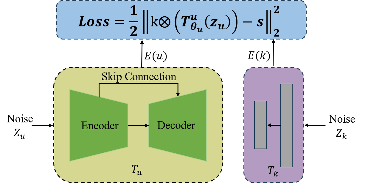
(a) Overview of the DIP [32].

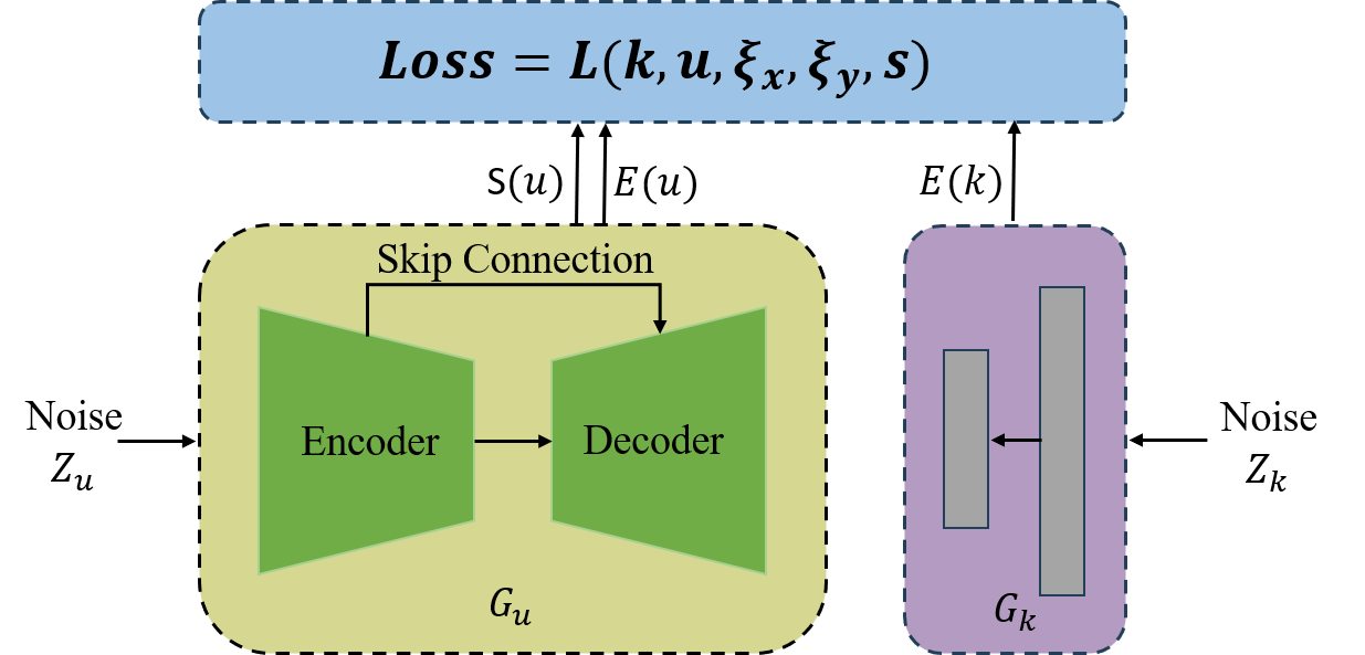
(b) Overview of the VDIP [33].

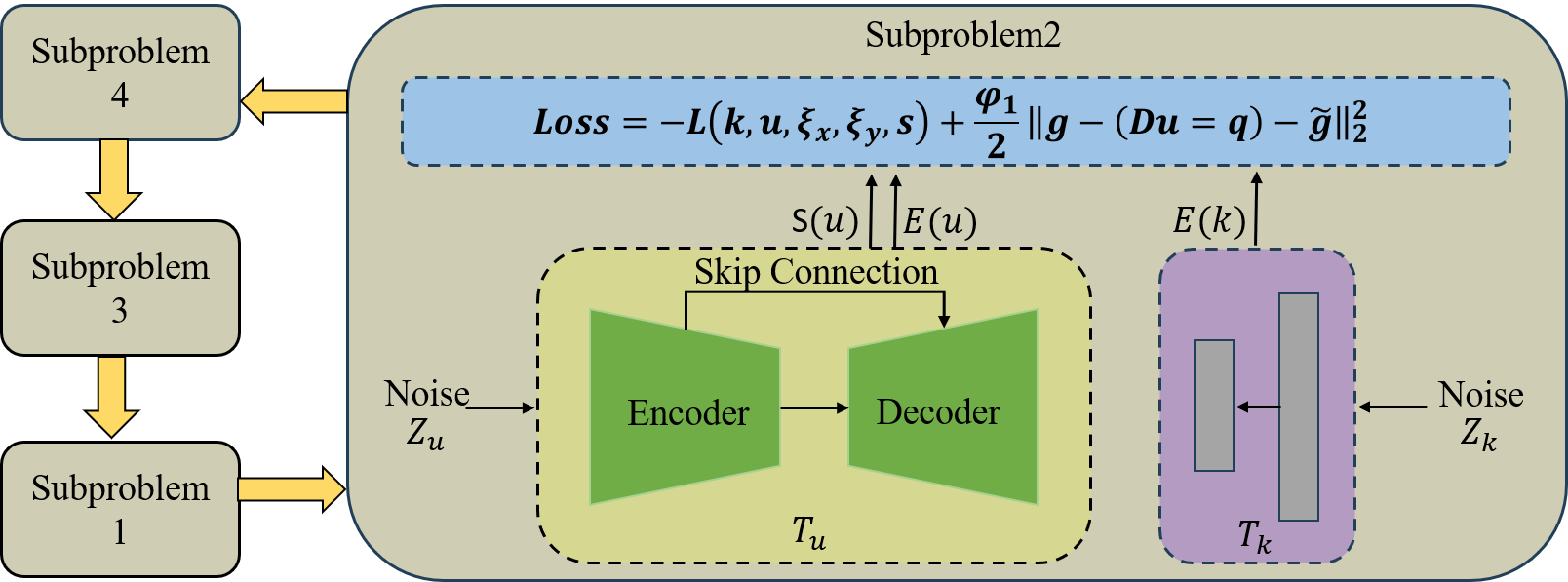
(c) Overview of our method.

(a)

Figure 1: The overview diagrams of DIP, VDIP, and the proposed VDIP-TGV. VDIP considers the effect of image variance, thereby bringing extra constraints relative to DIP. Details of the loss function of subgraph (b) can be found in Section III-A. We introduce TGV regularization on the basis of VDIP. According to the ADMM algorithm, the four sub-problems are solved successively, and the yellow arrow indicates the outer loop. Details of the loss function for subgraph (c) are shown in Section IV-B.

To overcome this issue, the VDIP [33] was proposed that employs a VB-based approach in DIP. The posterior distribution $P$ is approximated using a trivial distribution $Q$ (e.g., Gaussian), and the distance measure is the KL divergence. The problem in Eq. (6) can be converted into the problem of minimizing the KL divergence

$$D_{KL}\left(Q\left(k,u,\xi_{x},\xi_{y}\right)\|P\left(k,u,\xi_{x},\xi_{y}\mid s\right)\right)$$ (10)

$$= \ln P\left(s\right)-\int Q\left(k\right)\ln\frac{P\left(k\right)}{Q\left(k\right)}dk+\int Q\left(u\right)\ln Q\left(u\right)du$$

$$-\int Q\left(u\right)Q\left(\xi_{x},\xi_{y}\right)\ln P\left(u\mid\xi_{x},\xi_{y}\right)dud\xi_{x}d\xi_{y}$$

$$-\int Q\left(\xi_{x},\xi_{y}\right)\ln\frac{P\left(\xi_{x},\xi_{y}\right)}{Q\left(\xi_{x},\xi_{y}\right)}d\xi_{x}d\xi_{y}$$

$$-E_{Q\left(u\right)}\left[\ln P\left(s\mid u,k\right)\right],$$

where $D_{KL}$ represents the KL divergence, $L\left(k,u,\xi_{x},\xi_{y},s\right)$ is the variational lower bound, $P(k)$ is set as the standard Gaussian distribution, and $\xi_{x}$ and $\xi_{y}$ are the variational parameters introduced for the convenience of calculation. The third line in Eq. (10) is easy to calculate because $\ln P(s)$ is constant, and other terms only relate to the Gaussian distribution. Gaussian distributions can simplify derivation and implementation due to the continuity of their derivatives. The last line can be calculated by Monte Carlo estimation [45]. However, the fourth and fifth lines are hard because we don’t know the distribution of $P\left(u\mid\xi_{x},\xi_{y}\right)$ and $P\left(\xi_{x},\xi_{y}\right)$. Thus $\xi_{x}$ and $\xi_{y}$ are introduced as variational parameters such that $P\left(u\mid\xi_{x},\xi_{y}\right)$ is Gaussian, and $\xi_{x}$ and $\xi_{y}$ are related to image $u$. Then the fourth line in Eq. (10) is easy to calculate because all terms are related to Gaussian distribution. The fifth line in Eq. (10) is also addressed because the integral operation whose variables involve only $\xi_{x}$ and $\xi_{y}$ can be ignored [33].

How the distribution of $P\left(u\mid\xi_{x},\xi_{y}\right)$ becomes Gaussian is explained as follows. The traditional image prior can be expressed as a super-Gaussian distribution, which can be expressed by the formula

$$\small P(u)=W\mathrm{exp}\left(-\frac{\rho(F_{x}(u))+\rho(F_{y}(u))}{2}\right),$$ (11)

where $W$ is the normalization coeffcient, and $\rho(\cdot)$ is the penalty function to constrain sparsity. $F_{x}(\cdot)$ and $F_{y}(\cdot)$ are gradient kernels $[-1,1]^{T}$ and $[-1,1]$. According to Babancan et al. [46], the upper bound of $\rho(F_{x}(u))$ and of $\rho(F_{y}(u))$ are represented as

$$\rho(F_{x}(u))\leq\frac{1}{2}\xi_{x}(F_{x}(u))^{2}-\rho^{*}(\frac{1}{2}\xi_{x}),$$ (12)

$$\rho(F_{y}(u))\leq\frac{1}{2}\xi_{y}(F_{y}(u))^{2}-\rho^{*}(\frac{1}{2}\xi_{y}),$$

where $\rho^{*}(\frac{1}{2}\xi_{x})$ and $\rho^{*}(\frac{1}{2}\xi_{y})$ denote the concave conjugates of $\rho(\sqrt{F_{x}(u)})$ and $\rho(\sqrt{F_{y}(u)})$, respectively, and $\xi_{x}$ and $\xi_{y}$ are the variational parameters. Since $\frac{1}{2}\xi_{x}(F_{x}(u))^{2}-\rho^{*}(\frac{1}{2}\xi_{x})$ and $\frac{1}{2}\xi_{y}(F_{y}(u))^{2}-\rho^{*}(\frac{1}{2}\xi_{y})$ are both convex quadratic function, both of them has global minimum. The equation in Eq. (12) holds true when

$$\small\xi_{x}=\frac{\rho^{{}^{\prime}}(F_{x}(u))}{\left|F_{x}(u)\right|},\xi_{y}=\frac{\rho^{{}^{\prime}}(F_{y}(u))}{\left|F_{y}(u)\right|},$$ (13)

where $\rho^{{}^{\prime}}(\cdot)$ is the dervation of $\rho(\cdot)$. If $u$ is determined, $\xi_{x}$ and $\xi_{y}$ can also be determined by $u$.

By replacing the $\rho(F_{x}(u))$ and $\rho(F_{y}(u))$ in Eq. (11) with the corresponding right half of Eq. (12), $P(u|\xi_{x},\xi_{y})$ becomes a trivial Gaussian distribution

$$P(u|\xi_{x},\xi_{y})= W\mathrm{exp}\left(-\frac{\xi_{x}(F_{x}(u))^{2}+\xi_{y}(F_{y}(u))^{2}}{4}\right)$$ (14)

$$\cdot\mathrm{exp}\left(-\frac{\rho^{*}(\frac{1}{2}\xi_{y})+\rho^{*}(\frac{1}{2}\xi_{y})}{2}\right).$$

Then according to Eq. (14), the fourth row of formula Eq. (10) is easy to calculate. Finally, aided by $\xi_{x}$ and $\xi_{y}$, the computational difficulties of Eq. (10) are solved.

According to Eq. (14) and (10), the variational lower bound $\mathcal{L}\left(k,u,\xi_{x},\xi_{y},s\right)$ can be rewritten as

$$\mathcal{L}\left(k,u,\xi_{x},\xi_{y},s\right)$$ (15)

$$= \frac{1}{2}\sum_{i=1}^{I}\sum_{j=1}^{J}(2\ln S(u(m,n)-E^{2}(k(i,j))-S^{2}(k(i,j)))$$

$$+\frac{1}{2}\sum_{m=1}^{k}\sum_{n=1}^{N}2\ln S\left(u(m,n)\right)$$

$$-\frac{1}{4}\sum_{m=1}^{k}\sum_{n=1}^{N}E\left(\left(F_{x}\left(u\right)(m,n)\right)^{2}\right)E\left(\xi_{x}(m,n)\right)$$

$$-\frac{1}{4}\sum_{m=1}^{k}\sum_{n=1}^{N}E\left(\left(F_{y}\left(u\right)(m,n)\right)^{2}\right)E\left(\xi_{y}(m,n)\right)$$

$$+E_{Q\left(u\right)}\left[\ln P\left(s\mid u,k\right)\right],$$

where $(i,j)$ denotes the pixel index of kernel $k$, $S(\cdot)$ and $E(\cdot)$ are the standard deviation and the expectation of distribution $Q(\cdot)$, respectively, $(m,n)$ is the pixel index of $u$ and variational parameters $\xi_{x}$ and $\xi_{y}$.

Given that $\ln P(s)$ remains constant and $D_{KL}$ holds a non-negative value in Eq. (10), the task of minimizing $D_{KL}$ is reduced to minimizing the $-\mathcal{L}\left(k,u,\xi_{x},\xi_{y},s\right)$. In order to better minimize $-\mathcal{L}\left(k,u,\xi_{x},\xi_{y},s\right)$, VDIP used a fully-connected network as the kernel generator $G_{k}$ to get the distribution of kernels (like $S(k)$) and an encoder-decoder as the image generator $G_{u}$ to get the distribution of clean images (like $S(u)$ and $E(u)$). The blind deblurring of VDIP can be represented by the following formula

$$\small\begin{cases}\theta_{u},\theta_{k}=\mathop{\arg\min}\limits_{\theta_{u},\theta_{k}}-\mathcal{L}\left(k,u,\xi_{x},\xi_{y},s\right),\\ u=T^{u}_{\theta_{u}}(z_{u}),k=T^{k}_{\theta_{k}}(z_{k}),\end{cases}$$ (16)

where $-\mathcal{L}\left(k,u,\xi_{x},\xi_{y},s\right)$ is the loss function, $z_{u}$ and $z_{k}$ are random noises fed into the image generator $T^{u}$ and the kernel generator $T^{k}$, respectively, and $\theta_{u}$ and $\theta_{k}$ are parameters of $T^{u}$ and $T^{k}$, respectively. The network architectures of $T^{u}$ and $T^{k}$ are the same as that of DIP in Eq. (9). A frame diagram of VDIP for image blind deconvolution can be seen in Fig. 1. Since VDIP imposes constraints on the generated images and kernels by taking into account the variance of the generated image, VDIP has a better deblurring effect than DIP.

III-B TGV Regularization

TGV regularization generalizes TV regularization [25] by addressing the step effect issue of TV [25]. It was demonstrated that TGV regularization can retain more texture information and generate more visually pleasing results than TV regularization. The TGV of the order $k$ is defined as

$${{\rm{TGV}}_{\gamma}^{k}(u)}= \text{sup}\{\int_{\Omega}u{\rm{div}}^{k}vdx\mid v\in C_{c}^{k}(\Omega,{\rm{Sym}}^{k}(\mathbb{R}^{d})),$$ (17)

$$\|{\rm div}^{l}v\|_{\infty}\leq\gamma_{l},l=0,\cdots,k-1\},$$

where ${\rm{Sym}}^{k}(\mathbb{R}^{d})$ denotes the space of symmetric tensors of the order $k$ with arguments in $\mathbb{R}^{d}$, and $\gamma_{l},l=0,\cdots,k-1$ are fixed positive parameters. TGV can be interpreted as a “sparse” penalization of optimal balancing from the first up to the $k-$th distributional derivative. Specially, when $k=1$, $\gamma=1$, $\rm TGV_{1}^{1}$ is equivalent to $\rm TV$ and when $k=2$ , $\gamma<0$,

$${{\rm{TGV}}_{\gamma}^{2}(u)}= \text{sup}\{\int_{\Omega}u{\rm{div}^{2}}\omega dx\mid\omega\in C_{c}^{2}(\Omega,S^{d*d}),$$ (18)

$$\|\omega\|_{\infty}\leq\gamma_{0},\|{\rm div}\omega\|_{\infty}\leq\gamma_{l},l=0,1,\cdots,k-1\},$$

which is called the second-order $\rm{TGV}$. In the case $k>2$, ${\rm TGV}_{\gamma}^{k}(u)$ is called the high-order $\rm{TGV}$. We have adopted the second-order TGV in our model due to the higher computational complexity involved with high-order $\rm{TGV}$, which involves the high-order divergence operators.

Since the $k$-th order TGV can be interpreted as a sparse penalization of optimal balancing from the first derivative to the $k$-th order derivative, the second-order TGV must contain the second-order derivative. Given an image $u$, $\operatorname{TGV}_{\gamma}^{2}(u)$ performs well in penalization of $\nabla^{2}u$ in homogenous regions because $\|\nabla^{2}u\|_{1}$ is considerably smaller than $\|\nabla u\|_{1}$, thus the undesirable noise and artifacts could be suppressed correspondingly in homogenous regions. In contrast, $\|\nabla^{2}u\|_{1}$ is significantly larger than $\|\nabla u\|_{1}$ in the neighborhood of edges. In this case, $\operatorname{TGV}_{\gamma}^{2}(u)$ has the capacity to suppress staircase-like artifacts and preserve sharp edges.

The digital representation of images is mostly discrete, so in order to better apply TGV regularization to image processing, discrete TGV is introduced. According to [47, 48], when $\operatorname{div}w=v$ in $(2)$, $U=C_{c}^{2}(\Omega,\mathbb{R})$, $V=C_{c}^{2}\left(\Omega,\mathbb{R}^{2}\right)$ and $W=C_{c}^{2}\left(\Omega,\rm S^{2\times 2}\right)$, the discretized ${\mathrm{TGV}}_{\gamma}^{2}$ can be written as

$$\operatorname{TGV}_{\gamma}^{2}(u)= \max_{v\in V,w\in W}\{\langle u,\operatorname{div}v\rangle\mid\operatorname{div}w=v,\|w\|_{\infty}\leq\gamma_{0},$$ (19)

$$\|v\|_{\infty}\leq\gamma_{1}\},$$

where $\operatorname{div}w=\left[\begin{array}[]{l}\partial_{x}w_{11}+\partial_{y}w_{12}\\ \partial_{x}w_{21}+\partial_{y}w_{22}\end{array}\right].$ The indicator function of a closed set $B$ can be defined as $\mathcal{I}_{B}=\begin{cases}0,&x\in B\\ \infty,&\text{ else }\end{cases}.$ Then according to the fact that $\mathcal{I}_{\{0\}}(\cdot)=-\min_{y}\langle y,\cdot\rangle$, the representation of the discrete $\mathrm{TGV}^{2}$ is as follows:

$$\operatorname{TGV}_{\gamma}^{2}(u)= \min_{q\in V}\max_{\begin{subarray}{c}\|w\|_{\infty}\leq\gamma_{0},w\in W\\ \|v\|_{\infty}\leq\gamma_{1},v\in V\end{subarray}}\langle u,\operatorname{div}v\rangle+\langle q,v-\operatorname{div}w\rangle$$ (20)

$$= \min_{q\in V}\max_{\begin{subarray}{c}\|w\|_{\infty}\leq\gamma_{0},w\in W\\ \|v\|_{\infty}\leq\gamma_{1},v\in V\end{subarray}}\langle-\nabla u,v\rangle+\langle q,v\rangle+\langle\overline{\mathcal{B}}(q),w\rangle.$$

Using the symmetry property of the constraint $\{\|v\|_{\infty}\leq\gamma_{1}\}$ about zero and replacing $v$ with $-v$, the discrete form of $\mathrm{TGV}^{2}$ finally becomes

$$\operatorname{TGV}_{\gamma}^{2}(u)= \min_{q\in V}\max_{\begin{subarray}{c}\|w\|_{\infty}\leq\gamma_{0},w\in W\\ \|v\|_{\infty}\leq\gamma_{1},v\in V\end{subarray}}\langle\nabla u-q,v\rangle+\langle\overline{\mathcal{B}}(q),w\rangle$$ (21)

$$= \min_{q\in V}\gamma_{1}\|\nabla u-q\|_{1}+\gamma_{0}\|\overline{\mathcal{B}}(q)\|_{1},$$

where the operators $\nabla$ and $\overline{\mathcal{B}}$ can be represented by

$$\small\begin{cases}&\nabla u=\left[\begin{array}[]{c}\nabla_{1}u\\ \nabla_{2}u\end{array}\right]=\left[\begin{array}[]{c}\partial_{x}u\\ \partial_{y}u\end{array}\right]\\ &\overline{\mathcal{B}}(q)=\left[\begin{array}[]{cc}\partial_{x}q_{1}&\frac{1}{2}\left(\partial_{y}q_{1}+\partial_{x}q_{2}\right)\\ \frac{1}{2}\left(\partial_{y}q_{1}+\partial_{x}q_{2}\right)&\partial_{y}q_{2}\end{array}\right].\end{cases}$$ (22)

III-C ADMM Algorithm

The ADMM algorithm [37, 38] is a classic approach for addressing optimization problems that have linear constraints. When faced with complex objective functions, it is challenging to find an optimal solution directly. However, by utilizing the ADMM algorithm, one can decompose a difficult optimization problem into a set of simpler sub-problems that can be iteratively solved to obtain the optimal solution. This process enables the ADMM algorithm to tackle challenging optimization problems. Typically, the optimization problems that ADMM algorithm can solve are

$$\small\begin{array}[]{l}\min\limits_{y,z}f_{1}(y)+f_{2}(z)\\ \text{s.t. }y+Az+B=0,\end{array}$$ (23)

where $y\in\mathbb{R}^{m}$, $z\in\mathbb{R}^{q}$, $A\in\mathbb{R}^{m\times q}$, $B\in\mathbb{R}^{m}$ , $f_{1}:\mathbb{R}^{p}\rightarrow\mathbb{R}$, $f_{2}:\mathbb{R}^{q}\rightarrow\mathbb{R}$. According to linear constraints $y+Az+B=0$, the Lagrange functional equation of the problem can be written as follows

$$\mathcal{L}_{\xi}(y,z,\lambda)= f_{1}(y)+f_{2}(z)+\frac{\xi}{2}\|y+Az+B\|_{2}^{2}$$ (24)

$$+\lambda^{\top}(y+Az+B),$$

where $\lambda\in\mathbb{R}^{k}$, $\lambda$ is referred to as the Lagrange multiplier and $\xi$ represents the penalty parameter. Then, the variables $y$,$z$ and $\psi$ are iteratively updated according to the following equation

$$y^{(k+1)}=\mathop{\arg\min}\limits_{y}f_{1}(y)+\frac{\xi}{2}\|y+Az^{k}+B+\psi^{k}\|_{2}^{2},$$ (25)

$$z^{(k+1)}=\mathop{\arg\min}\limits_{z}f_{2}(z)+\frac{\xi}{2}\|y^{k+1}+Az+B+\psi^{k}\|_{2}^{2},$$

$$\psi^{(k+1)}=\psi^{(k)}+y^{(k+1)}+Az^{(k+1)}+B,$$

where $\psi=\frac{\xi}{\lambda}$. Lastly, the best solution for $y$ and $z$ can be obtained by continuously updating $y$, $z$ and $\psi$ alternatively.

IV Our Model

Here, we propose a single-image blind deconvolution model by combining VDIP and TGV. The loss function comes from the derivation of the VB. Our method is different from DIP-based methods. While several DIP-based methods have explored combining DIP with regularization, such as DIP-TV [40] and DIP-VBTV [35], to the best of our knowledge, no one has so far attempted to combine the VDIP with any forms of regularization for single-image blind deconvolution. Moreover, adding the TGV regularization into VDIP preserves details and captures more information when the blur kernel is large and the image size is small.

The ADMM algorithm is used to solve the model, and it transforms the problem into solving 4 sub-problems, in which two networks $T^{u}$ (capturing the prior information of clean images) and $T^{k}$ (capturing the prior information to blur kernels) are trained to solve the second sub-problem. Two networks share a loss function and update iteratively at the same time. The optimization strategy we provide can be thought of as a major modification of [49]. [49] utilizes a pre-trained GAN in conjunction with a prior $R(z)$, and solves the resulting optimization problem through the ADMM algorithm. One key difference between our approach and previous deep learning-based methods like [49] is that we achieve high-quality results without the need for large datasets or extensive training. Traditional variational models have typically not incorporated neural networks in conjunction with the ADMM algorithm, whereas our approach leverages them to significantly enhance image quality. Specifically, we adapt the objective function of a subproblem in the ADMM algorithm as the loss function according to the VB method. The overview of our method is clearly displayed in Fig. 1.

IV-A VDIP-TGV

In this paper, we propose a general single-image blind deconvolution model called VDIP-TGV, which combines the penalty term ${\rm TGV}_{\gamma}^{2}(u)$ and the fidelity term ${\|k\otimes u-s\|}^{2}_{2}$. According to Eq. (21) for the second-order TGV, the objective function in Eq. (6) can be rewritten as

$$\small\mathop{\min}\limits_{u,k}\frac{\beta}{2}\|k\otimes u-s\|^{2}_{2}+{\rm TGV}_{\gamma}^{2}(u),$$ (26)

where ${\rm TGV}_{\gamma}^{2}(u)=\gamma_{1}\|\nabla u-q\|_{1}+\gamma_{0}\|\overline{\mathcal{B}}(q)\|_{1}$, and $\gamma_{1}$ and $\gamma_{0}$ are positive numbers. In order to facilitate the calculation, we approximate directional derivatives $\nabla_{1}^{u}$ and $\nabla_{2}^{u}$ in Eq. (22) by $D_{1}^{u}$ and $D_{2}^{u}$ like [48], where $D_{1}^{u}$ and $D_{2}^{u}$ are the forward finite difference operators along the $x$ axis and $y$ axis, respectively. After replacing $\nabla u$ with $Du$ and approximating $\overline{\mathcal{B}}(q)$ by $\mathcal{B}(q)$, Eq. (22) can be rewritten as

$$\small\begin{cases}&Du=\left[\begin{array}[]{c}D_{1}u\\ D_{2}u\end{array}\right],\\ &\mathcal{B}(q)=\left[\begin{array}[]{cc}D_{1}q_{1}&\frac{1}{2}\left(D_{2}q_{1}+D_{1}q_{2}\right)\\ \frac{1}{2}\left(D_{2}q_{1}+D_{1}q_{2}\right)&D_{2}q_{2}\end{array}\right].\end{cases}$$ (27)

Our approach uses a generator $T^{u}_{\theta_{u}}$ to estimate blur kernels and a generator $T^{k}_{\theta_{k}}$ to estimate clean images. The network structures of both generators are the same as those of VDIP. The procedure for solving our method can be written as

$$\small\begin{cases}\theta_{u},\theta_{k}=\mathop{\arg\min}\limits_{\theta_{u},\theta_{k}}\frac{\beta}{2}\|k\otimes u-s\|^{2}_{2}+{\rm TGV}_{\gamma}^{2}(u),\\ {\rm TGV}_{\gamma}^{2}(u)=\gamma_{1}\|Du-q\|_{1}+\gamma_{0}\|\mathcal{B}(q)\|_{1},\gamma_{1}>0,\gamma_{0}>0,\\ u=T^{u}_{\theta_{u}}(z_{u}),k=T^{k}_{\theta_{k}}(z_{k}),\end{cases}$$ (28)

where $z_{u}$ and $z_{k}$ are the inputs of $T^{u}$ with parameters $\theta_{u}$ and $T^{k}$ with parameters $\theta_{k}$, respectively. Treating the objective function of the first row in Eq. (28) as a loss function like DIP and VDIP does not work because it is difficult to calculate $q$ according to the output of each iteration ($u$). Considering that the ADMM algorithm is famous for dividing and conquering the complex problem, we use the ADMM algorithm to solve the objective function.

IV-B Optimizing VDIP-TGV

Algorithm 1 gives a brief summary of our optimization strategy. According to the ADMM algorithm, we introduce auxiliary variables:

$$g=\left[\begin{array}[]{cc}g_{1}\\ g_{2}\end{array}\right]\in V, h=\left[\begin{array}[]{cc}h_{1}&h_{3}\\ h_{3}&h_{2}\end{array}\right]\in W,$$

where $V=C_{c}^{2}\left(\Omega,\mathbb{R}^{2}\right)$ and $W=C_{c}^{2}\left(\Omega,\rm S^{2\times 2}\right)$, and rewrite Eq. (26) as

$$\underset{g,h,u,q}{\text{min}}\frac{\beta}{2}\|k\otimes u-s\|_{2}^{2}+\gamma_{1}\|g\|_{1}+\gamma_{0}\|h\|_{1}$$ (29)

$$\text{ s.t. }g=Du-q,h=\mathcal{B}(q).$$

Then after introducing the Lagrangian multipliers $\widetilde{g}$, $\widetilde{h}$ and penalty parameters $\varphi_{1}$, $\varphi_{2}>0$, and denoting $\widetilde{g}=\frac{\varphi_{1}}{g}$, $\widetilde{h}=\frac{\varphi_{2}}{h}$, the augmented Lagrangian equation for the aforementioned minimization issue (29) is therefore obtained as follows:

$$\underset{g,h,u,q}{\text{min}}\frac{\beta}{2}\|k\otimes u-s\|_{2}^{2}+\gamma_{1}\|g\|_{1}+\gamma_{0}\|h\|_{1}$$ (30)

$$+\frac{\varphi_{1}}{2}\|g-(Du-q)-\widetilde{g}\|_{2}^{2}+\frac{\varphi_{2}}{2}\|h-\mathcal{B}(q)-\widetilde{h}\|_{2}^{2}.$$

Finally, the following five subproblems are resolved alternatively to arrive at the optimal solution.

$\bullet$ $g$-subproblem

$$\small g^{n+1}=\mathop{\arg\min}\limits_{g}\gamma_{1}\|g\|_{1}+\frac{\varphi_{1}}{2}\|g-(Du^{n}-q^{n})-\widetilde{g}^{n}\|_{2}^{2}.$$ (31)

Since the $g$-subproblem is elementwise separable, the solution to the $g$-subproblem reads as

$$\small g^{n+1}(l)=\gamma_{1}(\mathcal{S}\mathcal{H}_{2}\left(Du^{n}(l)-q^{n}(l)+\tilde{g}^{n}(l),\gamma_{1}/\varphi_{1}\right)),\quad l\in\Omega,$$ (32)

where $g^{n+1}(l)$ represents $g^{n+1}$ located at $l\in\Omega$, and the isotropic shrinkage operator $\mathcal{S}\mathcal{H}_{2}(a,\varphi)$ is defined as

$$\small\mathcal{S}\mathcal{H}_{2}(a,\varphi)=\begin{cases}0,&a=0,\\ \left(\|a\|_{2}-\varphi\right)\frac{a}{\|a\|_{2}},&a\neq 0.\end{cases}$$

$\bullet$ $h$-subproblem

$$\small h^{n+1}=\mathop{\arg\min}\limits_{h}\gamma_{0}\|h\|_{1}+\frac{\varphi_{2}}{2}\|h-(\mathcal{B}(q^{n}))-\widetilde{h}^{n}\|_{2}^{2}.$$ (33)

Likewise, the solution to the $h$-subproblem is as follows

$$\small h^{n+1}(l)=\gamma_{0}(\mathcal{S}_{F}(\mathcal{B}\left(q^{n}\right)(l)+\tilde{h}^{n}(l),\gamma_{0}/\varphi_{2})),\quad l\in\Omega,$$ (34)

where $h^{n+1}(l)\in{\rm{S}}^{2*2}$ is the component of $h^{n+1}$corresponding to the pixel $l\in\Omega$ and

$$\small\mathcal{S}_{F}(b,\varphi)=\begin{cases}0,&b=0,\\ \left(\|b\|_{F}-\varphi\right)\frac{b}{\|b\|_{F}},&b\neq 0.\end{cases}$$

$\bullet$ $u$-subproblem

$$\small u^{n+1}=\mathop{\arg\min}\limits_{u}\frac{\beta}{2}\|k\otimes u-s\|_{2}^{2}+\frac{\varphi_{1}}{2}\|g^{n+1}-(Du-q^{n})-\widetilde{g}^{n}\|_{2}^{2}.$$ (35)

In order to solve this objective function, we split it into two parts: $\frac{\beta}{2}\|k\otimes u-s\|_{2}^{2}$ and the rest. Drawing inspiration from the VDIP, we minimize the first part using the VB approach so that we could take advantage of the variance constraints of the images to avoid the issues of sparse MAP. VB involves utilizing a simple distribution, such as a Gaussian distribution, denoted as $Q(k,u,\xi_{x},\xi_{y})$, to approximate the posterior distribution $P(k,u,\xi_{x},\xi_{y}\|s)$. This approximation is achieved by minimizing the KL divergence, as represented in Eq. (10). Then minimizing the first part in Eq. (35) is equivalent to minimizing the term $-\mathcal{L}\left(k,u,\xi_{x},\xi_{y},s\right)$ in Eq. (10). Since solving the $u$ subproblem is equivalent to minimizing the sum of $-\mathcal{L}\left(k,u,\xi_{x},\xi_{y},s\right)$ and the second part, the sum of $-\mathcal{L}\left(k,u,\xi_{x},\xi_{y},s\right)$ and the second part is viewed as our loss function. After a few iterations, we can get the output of the network, which is the solution to the $u$-subproblem. The $u$-subproblem’s resolution procedure is as follows:

$$\small\begin{cases}\begin{aligned} \theta_{u},\theta_{k}=&\mathop{\arg\min}\limits_{\theta_{u},\theta_{k}}-\mathcal{L}\left(k,u,\xi_{x},\xi_{y},s\right)\\ &+\frac{\varphi_{1}}{2}\|g^{n+1}-(Du-q^{n})-\widetilde{g}^{n}\|_{2}^{2},\end{aligned}\\ u=T^{u}_{\theta_{u}}(z_{u}),k=T^{k}_{\theta_{k}}(z_{k}),\end{cases}$$ (36)

from the corresponding subproblem. The network architectures of $T^{u}$ and $T^{k}$ are the same as those of VDIP in Eq. (16), which can be seen in Fig. 2.

$\bullet$ $q_{1}$ and $q_{2}$-subproblems

$$q^{n+1}= \mathop{\arg\min}\limits_{q}\frac{\varphi_{1}}{2}\|g^{n+1}-(Du^{n+1}-q)-\widetilde{g}^{n}\|_{2}^{2}$$ (37)

$$+\frac{\varphi_{2}}{2}\|h^{n+1}-\mathcal{B}(q)-\widetilde{h}^{n}\|_{2}^{2}.$$

After taking the derivative of the objective function of this subproblem and setting it to 0, we can get the following equation

$$\small\left\{\begin{aligned} 0=&\gamma_{1}\varphi_{1}(q_{1}-D_{1}u^{n+1}+g_{1}^{n+1}-\widetilde{g}_{1}^{n})\\ &+\gamma_{0}\varphi_{2}(D_{1}^{T}(D_{1}q_{1}-h_{1}^{n+1}+\widetilde{h}_{1}^{n})\\ &+\frac{1}{2}D_{2}^{T}(D_{2}q_{1}+D_{1}q_{2}-2h_{3}^{n+1}+2\widetilde{h}_{3}^{n})),\\ 0=&\gamma_{1}\varphi_{1}(q_{2}-D_{2}u^{n+1}+g_{2}^{n+1}-\widetilde{g}_{2}^{n})\\ &+\gamma_{0}\varphi_{2}(D_{2}^{T}(D_{2}q_{2}-h_{2}^{n+1}+\widetilde{h}_{2}^{n})\\ &+\frac{1}{2}D_{1}^{T}(D_{1}q_{2}+D_{2}q_{1}-2h_{3}^{n+1}+2\widetilde{h}_{3}^{n})).\end{aligned}\right.$$ (38)

After the transformation and basic arithmetic, we have

$$\small\left\{\begin{aligned} q_{1}=&\frac{k_{1}}{k_{2}},q_{2}=\frac{k_{3}}{k_{4}},\\ k_{1}=&\gamma_{1}\varphi_{1}(D_{1}u^{n+1}-g_{1}^{n+1}+\widetilde{g}_{1}^{n})+\gamma_{0}\varphi_{2}(D_{1}^{T}(h_{1}^{n+1}-\widetilde{h}_{1}^{n})\\ +&D_{2}^{T}(h_{3}^{n+1}-\widetilde{h}_{3}^{n}-\frac{1}{2}D_{1}q_{2}^{n})),\\ k_{2}=&{\gamma_{1}\varphi_{1}+\gamma_{0}\varphi_{2}(D_{1}^{T}D_{1}+\frac{1}{2}D_{2}^{T}D_{2})},\\ k_{3}=&\gamma_{1}\varphi_{1}(D_{2}u^{n+1}-g_{2}^{n+1}+\widetilde{g}_{2}^{n})+\gamma_{0}\varphi_{2}(D_{2}^{T}(h_{2}^{n+1}-\widetilde{h}_{2}^{n})\\ +&D_{1}^{T}(h_{3}^{n+1}-\widetilde{h}_{3}^{n}-\frac{1}{2}D_{2}q_{1}^{n})),\\ k_{4}=&{\gamma_{1}\varphi_{1}+\gamma_{0}\varphi_{2}(D_{2}^{T}D_{2}+\frac{1}{2}D_{1}^{T}D_{1})}.\end{aligned}\right.$$ (39)

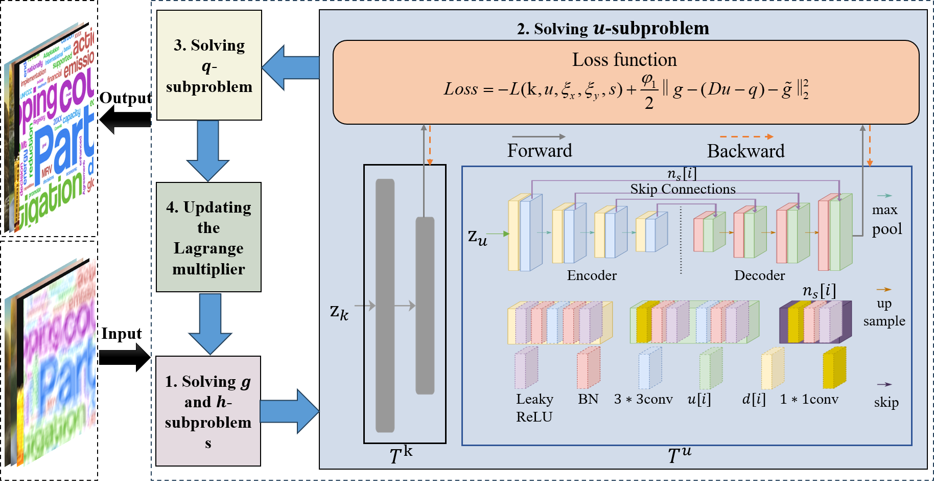
Figure 2: The flowchart of the proposed VDIP-TGV. The ADMM algorithm transforms the problem into solving 4 sub-problems, in which two networks $T^{u}$ (which captures the prior information for clean images) and $T^{k}$ (which captures the prior information for blur kernel) are used to solve the second sub-problem. The inputs to $T^{u}$ and $T^{k}$ are randomly initialized noise images, denoted by the symbols $z_{u}$ and $z_{k}$, respectively. The network architecture of $T^{u}$ is the same as that of the VDIP and DIP, using an autoencoder to output the deblurred image. $T^{k}$ uses a fully connected layer to output blur kernel, which is the same as VDIP. Both $T^{u}$ and $T^{k}$ use the same loss function. The determination of the loss function is based on the VB method, see Section IV-B for details.

$\bullet$ $\widetilde{g}$ and $\widetilde{h}$-subproblems

The Lagrange multipliers are updated as follows

$$\small\left\{\begin{aligned} \widetilde{g}^{n+1}&=\widetilde{g}^{n}+\mu(Du^{n+1}-q^{n+1}-g^{n+1}),\\ \widetilde{h}^{n+1}&=\widetilde{h}^{n}+\mu(\mathcal{B}(q^{n+1})-h^{n+1}).\end{aligned}\right.$$ (40)

By iteratively updating $g$, $h$, $u$, $p$ and Lagrange multipliers $\widetilde{g}$ and $\widetilde{h}$, the optimal solution $u$ is obtained.

Algorithm 1

1:  Choose $\gamma_{0}$, $\gamma_{1}$, $\varphi_{1}$, $\varphi_{2}$, $\beta$, $\mu$; Initialize $u_{0}$, $q_{1}^{0}$, $q_{2}^{0}$, $g_{j}^{0}$; $\widetilde{g}_{j}^{0}$, $(j=1,2)$, $h_{j}^{0}$, $\widetilde{h}_{j}^{0},(j=1,2,3)$; Set $t$ as the maximum number of iterations.

2:  for all $n=0,1,2,3,...,t$ do

3:     Update $g^{n}$ based on Eq. (32);

4:     Update $h^{n}$ based on Eq. (33);

5:     Update $k^{n}$ and $u^{n}$ based on Eq. (36);

6:     Update $q_{1}^{n}$, $q_{2}^{n}$ based on Eq. (39);

7:     Update $\widetilde{g}^{n}$, $\widetilde{h}^{n}$ based on Eq. (40);

8:     $n=n+1$.

9:  end for

10:  $U=u^{n}$.

11:  return  $U$.

V Experiment

In this section, we provide systematic quantitative and qualitative experiments to showcase the efficacy of our approach relative to other state-of-the-art methods.

V-A Implementation Details

Blur

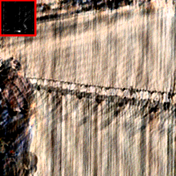
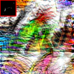
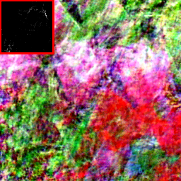
Ren et al. DIP [32]

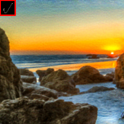
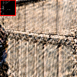
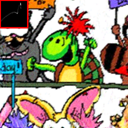
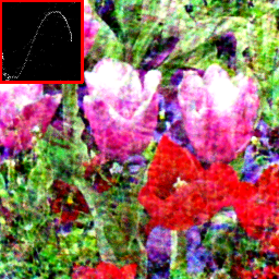
Dong et al. VDIP[33]

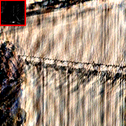
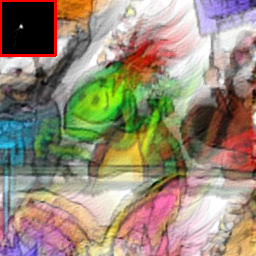
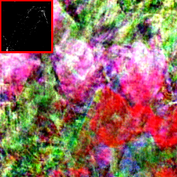
DIP-TGV

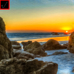
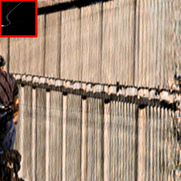
OURS (VDIP-TGV)

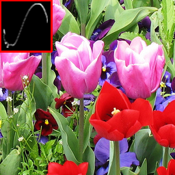
Clean

Figure 3: Qualitative comparisons between DIP-TGV and VDIP-TGV on four images.

Datasets. The experiment was conducted on two datasets, the dataset collected by Lai et al. [50] and the dataset collected by Kohler et al. [51]. The dataset collected by Lai et al. [50] includes 200 images, 100 of which are synthetic images and the rest are real images. The 100 synthetic images are convolved by four different sizes of blur kernels. These images belong to different categories such as Manmade, Natural, People, Saturated, and Text. The dataset collected by Kohler et al. [51] is made by randomly selecting 12 blurry trajectories that imitate the camera shake, and applying them to 4 images, resulting in 48 blurry images.

Methods. We contrast our proposed VDIP-TGV with several other methods, including conventional methods such as Krishnan et al. [52], Pan et al. [53], Wen et al. [54], deep learning-based methods such as Kupyn et al. [55], Zamir et al. [56] and Chen et al. [57], and DIP-based methods such as DIP [32] and VDIP [33]. All these works were published in flagship journals in the field of image processing.

Evaluation metrics. We use both reference and no-reference image quantitative assessment metrics to evaluate our algorithm. For reference metrics, we use Peak Signal-to-Noise Ratio (PSNR), Structural Similarity Index Measurement (SSIM) [58], and Mean Squared Error (MSE) [59]. When the PSNR value is larger or the SSIM value is closer to 1, the image quality after deblurring is considered to be higher. The smaller the error is, the more accurate the estimation of blur kernel is. For no-reference assessment metrics, we use Naturalness Image Quality Evaluator (NIQE) [60], Blind/Referenceless Image Spatial Quality Evaluator (BRISQUE) [61], and Perception based Image Quality EvaluatorPIQE (PIQE) [62]. The smaller the three indicators, the better quality the images have.

Setting. Our method uses networks $T^{u}$ and $T^{k}$ to capture the prior information for clean images and blur kernels, respectively. For a fair comparison, the architectures of $T^{u}$ and $T^{k}$ used in VDIP-TGV are the same as those in VDIP, where $T^{u}$ uses the autoencoder to yield a deblurring image, $T^{k}$ uses the fully connected layer to estimate a blur kernel, and the structural details of $T^{u}$ and $T^{k}$ can be seen in Fig 2. Similar to DIP [32] and VDIP [33], the total count of iterative steps is prescribed as 5,000 and the learning rate of the image generator and of the kernel generator are set as $1\times 10^{-2}$ and $1\times 10^{-4}$, respectively. All experiments are conducted using PyCharm 2021 on a PC equipped with an Intel Core i7-RTX 3050 on Windows 10.

V-B Analyzing the Effectiveness of VDIP-TGV

The highlight of our method is the employment of VDIP and the introduction of TGV. To confirm the effectiveness of VDIP-TGV, we compare VDIP-TGV with DIP [32], VDIP [33], and DIP-TGV. We randomly select 4 blurry images from Lai et al. [50] convoluted by kernels of different sizes for visualization and perform numerical experiments on them. The recovery images are shown in Fig. 3, and the numerical results are included in Tab. I. For a unified presentation, we select test images by cropping $256\times 256$ pixels from the middle of the original test images.

Real

Zamir et al. [56]

Krishnan et al. [52]

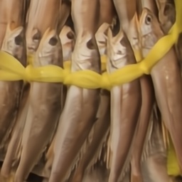
Chen et al. [57]

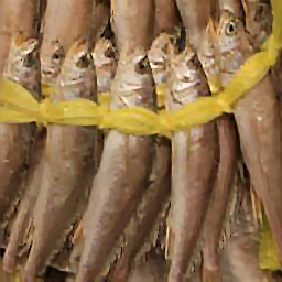
Pan et al. [53]

Ren et al. DIP[32]

Kupyn et al. [55]

Dong et al. VDIP[33]

Wen et al. [54]

OURS

Figure 4: Qualitative comparison of different methods on the real image dataset collected by Lai et al. [50].

Several conclusions can be drawn from Fig. 3. First, it is difficult for DIP to accurately estimate blur kernels from the limited amount of information, especially when the size of blur kernels is large (the last row in Fig. 3). DIP’s recovery is over-sharpened, and its estimation of blur kernels is also significantly inaccurate, except when the size of the blur kernel is small (the first row in Fig. 3). This is because DIP does not use the variance of pixels to establish constraints as VDIP does, nor does it use gradients to grasp more details as TGV does. Second, the experimental results of VDIP are somewhat unstable due to the absence of TGV constraints. In Fig. 3, the results of VDIP in the second and fourth rows are significantly over-sharpened, while the results of VDIP in the first and third rows have some unnatural artifacts. Third, DIP-TGV sometimes has the problem of the sparse MAP. As shown in the third row of Fig. 3, DIP-TGV obviously is cursed by the sparse MAP, and the estimated blur kernel was also a delta kernel. When the sparse MAP problem is not generated, DIP-TGV generates similar or slightly better results than DIP, which also indicates that the effect of combining DIP and TGV is not as good as that of combining VDIP and TGV. When VDIP and TGV are combined, the deblurring effect is the best. Finally, regardless the sizes of blur kernels, our method can accurately estimate the blur kernels from images.

V-C Comparatitive Experiments

TABLE I: Comparison of PSNR$\uparrow$ and SSIM$\uparrow$ values on the synthetic dataset from Lai et al. [50].

	Manmade	Natural	People	Saturated	Text	Average
Krishnan et al. [52]	17.70 / 0.463	17.69 / 0.465	17.62 / 0.460	17.51 / 0.452	17.66 / 0.458	17.64 / 0.459
Pan et al. [53]	17.84 / 0.483	17.57 / 0.484	17.23 / 0.476	17.10 / 0.473	17.49 / 0.501	17.45 / 0.483
Kupyn et al. [55]	17.75 / 0.458	17.79 / 0.456	18.00 / 0.462	18.10 / 0.469	18.12 /0.477	17.95 / 0.464
Wen et al. [54]	17.47 / 0.498	17.41 / 0.496	17.23 / 0.430	17.22 / 0.479	16.88 / 0.452	17.24 / 0.477
Zamir et al. [56]	17.21 / 0.455	17.52 / 0.456	17.90 / 0.472	18.04 / 0.481	17.86 / 0.479	17.71 / 0.469
Chen et al. [57]	16.77 / 0.266	18.39 / 0.369	19.84 / 0.485	18.69 / 0.496	17.76 / 0.465	18.29 / 0.416
Ren et al. DIP[32]	16.08 / 0.280	18.85 / 0.407	20.64 / 0.476	19.83 / 0.508	20.34 / 0.547	19.15 / 0.444
Dong et al. VDIP[33]	16.86 / 0.308	19.67 / 0.435	22.24 / 0.531	21.11 / 0.561	21.26 / 0.574	20.23 / 0.482
DIP-TGV	16.16 / 0.284	18.98 / 0.420	20.45 / 0.472	19.61 / 0.505	19.85 / 0.534	19.01 / 0.443
OURS	16.94 / 0.315	20.15 / 0.466	22.64 / 0.559	21.40 / 0.578	21.51 / 0.595	20.53 / 0.503

TABLE II: Comparison of average kernel recovery error$\downarrow$ on the synthetic dataset from Lai et al. [50].

	Manmade	Natural	People	Saturated	Text	Average
Krishnan et al. [52]	0.01559	0.01559	0.0156	0.01562	0.01560	0.01560
Pan et al. [53]	0.02601	0.02471	0.02603	0.02218	0.02127	0.02404
Wen et al. [54]	0.02341	0.02613	0.02608	0.01987	0.02130	0.02336
Ren et al. DIP[32]	0.01827	0.01706	0.01688	0.01560	0.01649	0.01686
Dong et al. VDIP[33]	0.02341	0.01614	0.01543	0.01580	0.01537	0.01723
DIP-TGV	0.02170	0.01725	0.01683	0.01614	0.01420	0.01722
OURS	0.01208	0.00955	0.00907	0.01070	0.00852	0.00998

Blurred

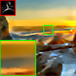
Pan et al. [53]

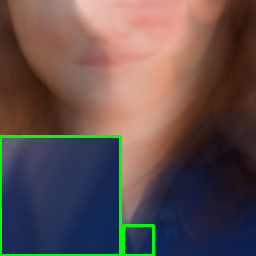
Blurred

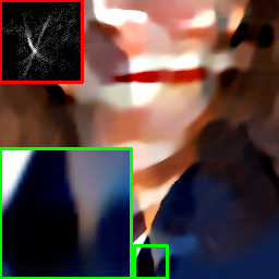
[53]

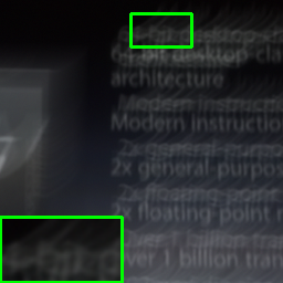
Blurred

[53]

Kupyn et al. [55]

Ren et al. DIP[32]

Kupyn et al. [55]

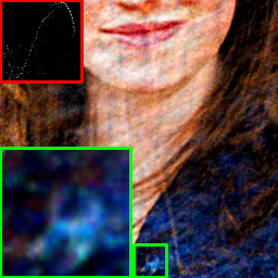
Ren et al. DIP[32]

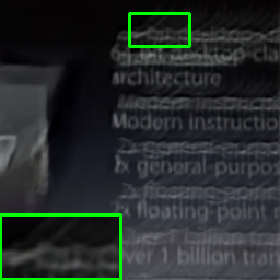
Kupyn et al. [55]

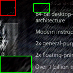
Ren et al. DIP[32]

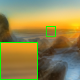
Zamir et al. [56]

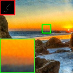
Dong et al. VDIP[33]

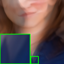
Zamir et al. [56]

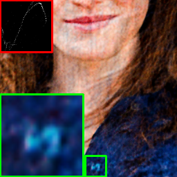
Dong et al. VDIP[33]

Zamir et al. [56]

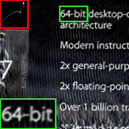
Dong et al. VDIP[33]

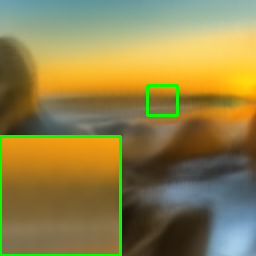
Chen et al. [57]

OURS

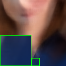
Chen et al. [57]

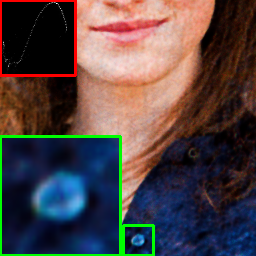
OURS

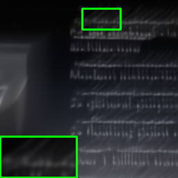
Chen et al. [57]

OURS

Wen et al. [54]

Clean

Wen et al. [54]

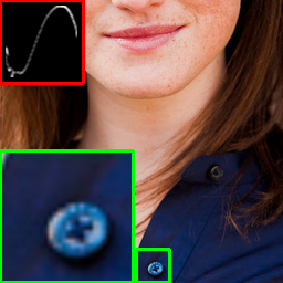
Clean

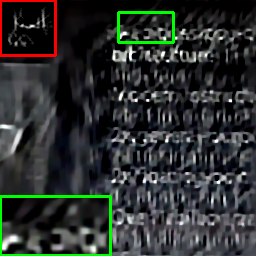
Wen et al. [54]

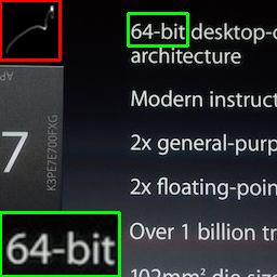
Clean

Figure 5: Qualitative comparison on the synthetic dataset from Lai et al. [50].

V-C1 Qualitative Comparison

To further demonstrate that our method can perform well in visual effects and retain more details, we visualize the recovered images as shown in Figs. 5 and 4 which are synthetic and real images, respectively. The estimated kernels are put in the upper left of the corresponding deblurring results, and the enlarged details are in the lower left. Since some deep learning-based methods simulate an end-to-end process and do not estimate the kernels, some deblurring results in Fig. 5 do not have kernels shown. Fig. 5 shows the deblurring results of different methods for three synthetic images (nature image, people image, and text image). From Fig. 5, we can see that our method is visually better and has fewer artifacts than the DIP method. In the deblurring results from traditional methods, many artifacts are over-enhanced and even mismatched. Deep learning-based methods are obviously not effective in deblurring, possibly because there is no sufficient data to train the model. As can be seen from the zoomed details of the natural image, our method yields significantly fewer artifacts and less noise. By examining the people image, it can be seen that the button details are only recovered by our method, thanks to the edge extraction ability of the TGV regularization. From the zoomed details, we observe that characters in the text image are also restored more clearly by our method. Inspecting the estimated blur kernels, we can also easily find that our method estimates the blur kernels most accurately.

Observing the deblurring effects on real images in Fig. 4, it can be found that deep learning-based methods either have no deblurring effect or generate too smooth images, while the traditional methods are mostly too enhanced. Moreover, the DIP-based methods produce more artifacts than our method. Therefore, we summarize that our approach works best visually, both for synthetic and real images.

V-C2 Quantitative Comparison

Blind deblurring data sets can be divided into three categories: synthetic images, simulated real images, and real images. The difference between simulated real images and synthetic images is that the blur kernel of the former is simulated to imitate the real camera shake, while the latter is not. For traditional methods, the well-performing prior to all three kinds of images is difficult to design. For deep learning methods, training on a dataset containing three types of images is very resource-intensive. As a result, there are few methods that work well on three datasets at the same time. The prior information required by our method can directly be obtained from the destroyed single image and the network structure, so our method can be well applied to all images. To prove the above point, we conduct quantitative experiments on all three types of image sets.

For synthetic images, we illustrate the superiority of our method by calculating three numerical indexes: PSNR, SSIM, and MSE. As shown in Tabs. I and II, the best results are bold-faced, and the second-best are underlined. On the dataset from Lai et al. [50], our method yields superior image quality. For all three indexes, our model outperforms other competitors. To evaluate the accuracy of the estimated kernels, we calculate the average MSE, and the results are shown in Tab. II. Because some end-to-end deep learning models do not estimate blur kernels, Tab. II excludes them. It can be seen from Tab. II that the blur kernels estimated by our model are the most accurate compared with other models. Additionally, the numerical results in Tab. I further demonstrate that only when VDIP and TGV are combined, the deblurring effect is the best. In Tab. I, the numerical effect of DIP-TGV is inferior to DIP, which may be related to the sparse MAP problem caused by DIP-TGV.

TABLE III: Comparison of PSNR$\uparrow$ and SSIM$\uparrow$ values on the dataset from Kohler et al. [51].

	PSNR	SSIM
Krishnan et al. [52]	23.19	0.779
Pan et al. [53]	26.21	0.839
Kupyn et al. [55]	25.06	0.806
Chen et al. [57]	25.31	0.805
Ren et al. DIP[32]	21.61	0.717
Dong et al. VDIP[33]	25.33	0.850
OURS	26.49	0.860

TABLE IV: Comparison of NIQE$\downarrow$, BRISQUE$\downarrow$ and PIQE$\downarrow$ values on the real blurred dataset from Lai et al. [50].

	NIQE	BRISQUE	PIQE	Average
Krishnan et al. [52]	8.8243	33.3825	51.2052	31.1373
Pan et al. [53]	7.6492	30.5786	61.6742	33.3007
Kupyn et al. [55]	4.8964	32.6875	42.5616	26.7152
Wen et al. [54]	8.4819	31.6044	52.5347	30.8737
Zamir et al. [56]	5.3565	36.9692	49.4281	30.5846
Chen et al. [57]	6.6433	39.4483	62.0968	36.0628
Ren et al. DIP[32]	6.5901	30.5180	35.4707	24.1929
Dong et al. VDIP[33]	5.5079	28.3879	32.7918	22.2292
OURS	5.4210	29.2051	31.8626	22.1629

For simulated real images, we conduct experiments on a benchmark dataset collected by Kohler et al. [51]. Although this dataset does not have the ground truth like the synthetic images, Kohler et al. devised some computational rules to compute PSNR and SSIM similarly. We use the same way as Kohler et al. to compute PSNR and SSIM. As can be seen from Tab. III, regardless of PSNR or SSIM, the image recovered by our method has the highest performance.

In order to further prove that our method is also applicable to real scenes, we conduct experiments on real images of the dataset (Lai et al. [50]). Since the real image has no ground truth, we utilize three no-reference image quality assessment metrics to quantitatively evaluate the results, as shown in Tab. IV. It is shown that from the angle of NIQE and PIQE, the image quality after deblurring by our method is the highest, while regarding BRISQUE, the image quality by our method is suboptimal. Overall speaking, our method is still the best.

In brief, our systematic experiments demonstrate that the deep learning-based models do not perform as well as our method, probably because deep learning-based models are highly dependent on a large number of image pairs for training. The traditional method is not as good as ours, either, because the constraints added by the traditional methods are not enough to capture all the information of the images, while our method uses TGV and VDIP, combining the best of two worlds to capture more complete information.

VI Conclusion

In this article, we have proposed a model called VDIP-TGV that can improve VDIP in a highly nontrivial manner by overcoming its two pitfalls. One is that the image will lose details and boundaries after deblurring, and the other is that when the blur kernel size is relatively large, the image will be excessively sharpened after deblurring. Then, we have used the ADMM algorithm to decompose the target problem into four sub-problems to solve. Finally, we have conducted systematic experiments to verify the superiority of our model qualitatively and quantitatively. Future work can be generalizing the proposed VDIP-TGV into other low-level computer vision problems.

Declaration of competing interest

The authors declare that they have no known competing financial interests or personal relationships that could have appeared to influence the work reported in this paper.

Tingting Wu received the B.S. and Ph.D. degrees in mathematics from Hunan University, Changsha, China, in 2006 and 2011, respectively. From 2015 to 2018, she was a Postdoctoral Researcher with the School of Mathematical Sciences, Nanjing Normal University, Nanjing, China. From 2016 to 2017, she was a Research Fellow with Nanyang Technological University, Singapore. She is currently an Associate Professor with the School of Science, Nanjing Uni versity of Posts and Telecommunications, Nanjing. Her research interests include variational methods for image processing and computer vision, optimization methods and their applications in sparse recovery, and regularized inverse problems.

Zhiyan Du received the B.S. degree in School of Mathematics and Statistics from the Huanghuai University, Zhumadian, China, in 2021. She is currently pursuing an M.S. degree from the School of Science, Nanjing University of Posts and Telecommunications, Nanjing, China. Her research interests include image processing and computer vision, machine learning, and inverse problems.

Fenglei Fan is a research assistant professor at Department of Mathematics, The Chinese University of Hong Kong. He received his PhD degree in Rensselaer Polytechnic Institute, US. His research interests lie in deep learning theory and methodology. He was the recipient of the IBM AI Horizon Fellowship and the 2021 International Neural Network Society Doctoral Dissertation Award.

Zhi Li obtained his Bachelor’s and Master’s degrees from the China University of Petroleum, Shandong, China in 2007 and 2010 respectively. He also completed his Master’s degree in Applied Science from Saint Mary’s University, Halifax, NS, Canada in 2012. He earned his Ph.D. from Hong Kong Baptist University in 2016 and subsequently held a postdoctoral position at Michigan State University, East Lansing, Ml, USA from 2016 to 2019. He currently holds the position of Associate Researcher at the Department of Computer Science and Technology, East China Normal University, Shanghai, China.

Tieyong Zeng received the B.S. degree from Peking University, Beijing, China, in 2000, the M.S degree from Ecole Polytechnique, Palaiseau, France, in 2004, and the Ph.D. degree from the University of Paris XIII, Paris, France, in 2007. He worked as a Post-Doctoral Researcher with ENS de Cachan, Cachan, France, from 2007 to 2008, and an Assistant/Associate Professor with Hong Kong Baptist University, Hong Kong, from 2008 to 2018. He is currently a Professor in the Department of Mathematics, The Chinese University of Hong Kong, Hong Kong. His research interests are image processing, machine learning, and scientific computing.

References

- [1] L. Lin and L. V. Wang, “The emerging role of photoacoustic imaging in clinical oncology,” Nature Reviews Clinical Oncology, vol. 19, no. 6, pp. 365–384, 2022.
- [2] F. Fan, M. Li, Y. Teng, and G. Wang, “Soft autoencoder and its wavelet adaptation interpretation,” IEEE Transactions on Computational Imaging, vol. 6, pp. 1245–1257, 2020.
- [3] Q. Shan, J. Jia, and A. Agarwala, “High-quality motion deblurring from a single image,” Acm Transactions on Graphics (tog), vol. 27, no. 3, pp. 1–10, 2008.
- [4] M. S. Almeida and L. B. Almeida, “Blind and semi-blind deblurring of natural images,” IEEE Transactions on Image Processing, vol. 19, no. 1, pp. 36–52, 2009.
- [5] S. Cho and S. Lee, “Fast motion deblurring,” in ACM SIGGRAPH Asia 2009 Papers, 2009, pp. 1–8.
- [6] J. Pan, R. Liu, Z. Su, and X. Gu, “Kernel estimation from salient structure for robust motion deblurring,” Signal Processing: Image Communication, vol. 28, no. 9, pp. 1156–1170, 2013.
- [7] Y.-L. You and M. Kaveh, “A regularization approach to joint blur identification and image restoration,” IEEE Transactions on Image Processing, vol. 5, no. 3, pp. 416–428, 1996.
- [8] T. F. Chan and C.-K. Wong, “Total variation blind deconvolution,” IEEE Transactions on Image Processing, vol. 7, no. 3, pp. 370–375, 1998.
- [9] J. Pan, D. Sun, H. Pfister, and M.-H. Yang, “Blind image deblurring using dark channel prior,” in Proceedings of the IEEE Conference on Computer Vision and Pattern Recognition, 2016, pp. 1628–1636.
- [10] D. Krishnan, T. Tay, and R. Fergus, “Blind deconvolution using a normalized sparsity measure,” in CVPR 2011. IEEE, 2011, pp. 233–240.
- [11] W.-Z. Shao, H.-B. Li, and M. Elad, “Bi-l0-l2-norm regularization for blind motion deblurring,” Journal of Visual Communication and Image Representation, vol. 33, pp. 42–59, 2015.
- [12] A. Levin, Y. Weiss, F. Durand, and W. T. Freeman, “Understanding and evaluating blind deconvolution algorithms,” in 2009 IEEE Conference on Computer Vision and Pattern Recognition. IEEE, 2009, pp. 1964–1971.
- [13] B. Luo, Z. Cheng, L. Xu, G. Zhang, and H. Li, “Blind image deblurring via superpixel segmentation prior,” IEEE Transactions on Circuits and Systems for Video Technology, vol. 32, no. 3, pp. 1467–1482, 2021.
- [14] S. D. Babacan, R. Molina, M. N. Do, and A. K. Katsaggelos, “Bayesian blind deconvolution with general sparse image priors,” in Computer Vision–ECCV 2012: 12th European Conference on Computer Vision, Florence, Italy, October 7-13, 2012, Proceedings, Part VI 12. Springer, 2012, pp. 341–355.
- [15] R. Fergus, B. Singh, A. Hertzmann, S. T. Roweis, and W. T. Freeman, “Removing camera shake from a single photograph,” in Acm Siggraph 2006 Papers, 2006, pp. 787–794.
- [16] A. Levin, Y. Weiss, F. Durand, and W. T. Freeman, “Understanding and evaluating blind deconvolution algorithms,” in 2009 IEEE Conference on Computer Vision and Pattern Recognition. IEEE, 2009, pp. 1964–1971.
- [17] D. Wipf and H. Zhang, “Revisiting bayesian blind deconvolution,” Journal of Machine Learning Research (JMLR), 2014.
- [18] A. Levin, Y. Weiss, F. Durand, and W. T. Freeman, “Understanding and evaluating blind deconvolution algorithms,” in 2009 IEEE Conference on Computer Vision and Pattern Recognition. IEEE, 2009, pp. 1964–1971.
- [19] J. Miskin and D. J. MacKay, “Ensemble learning for blind image separation and deconvolution,” in Advances in Independent Component Analysis. Springer, 2000, pp. 123–141.
- [20] A. Levin, Y. Weiss, F. Durand, and W. T. Freeman, “Understanding blind deconvolution algorithms,” IEEE Transactions on Pattern Analysis and Machine Intelligence, vol. 33, no. 12, pp. 2354–2367, 2011.
- [21] J. Sun, W. Cao, Z. Xu, and J. Ponce, “Learning a convolutional neural network for non-uniform motion blur removal,” in Proceedings of the IEEE Conference on Computer Vision and Pattern Recognition, 2015, pp. 769–777.
- [22] A. Chakrabarti, “A neural approach to blind motion deblurring,” in Computer Vision–ECCV 2016: 14th European Conference, Amsterdam, The Netherlands, October 11-14, 2016, Proceedings, Part III 14. Springer, 2016, pp. 221–235.
- [23] L. Xu, J. S. Ren, C. Liu, and J. Jia, “Deep convolutional neural network for image deconvolution,” Advances in Neural Information Processing Systems, vol. 27, 2014.
- [24] X. Tao, H. Gao, X. Shen, J. Wang, and J. Jia, “Scale-recurrent network for deep image deblurring,” in Proceedings of the IEEE Conference on Computer Vision and Pattern Recognition, 2018, pp. 8174–8182.
- [25] S. Nah, T. Hyun Kim, and K. Mu Lee, “Deep multi-scale convolutional neural network for dynamic scene deblurring,” in Proceedings of the IEEE Conference on Computer Vision and Pattern Recognition, 2017, pp. 3883–3891.
- [26] O. Kupyn, T. Martyniuk, J. Wu, and Z. Wang, “Deblurgan-v2: Deblurring (orders-of-magnitude) faster and better,” in Proceedings of the IEEE/CVF International Conference on Computer Vision, 2019, pp. 8878–8887.
- [27] S.-J. Cho, S.-W. Ji, J.-P. Hong, S.-W. Jung, and S.-J. Ko, “Rethinking coarse-to-fine approach in single image deblurring,” in Proceedings of the IEEE/CVF International Conference on Computer Vision, 2021, pp. 4641–4650.
- [28] Z. Wang, X. Cun, J. Bao, W. Zhou, J. Liu, and H. Li, “Uformer: A general u-shaped transformer for image restoration,” in Proceedings of the IEEE/CVF Conference on Computer Vision and Pattern Recognition, 2022, pp. 17 683–17 693.
- [29] S. Wan, S. Tang, X. Xie, J. Gu, R. Huang, B. Ma, and L. Luo, “Deep convolutional-neural-network-based channel attention for single image dynamic scene blind deblurring,” IEEE Transactions on Circuits and Systems for Video Technology, vol. 31, no. 8, pp. 2994–3009, 2020.
- [30] Y. Mao, Z. Wan, Y. Dai, and X. Yu, “Deep idempotent network for efficient single image blind deblurring,” IEEE Transactions on Circuits and Systems for Video Technology, vol. 33, no. 1, pp. 172–185, 2022.
- [31] D. Ulyanov, A. Vedaldi, and V. Lempitsky, “Deep image prior,” in Proceedings of the IEEE Conference on Computer Vision and Pattern Recognition, 2018, pp. 9446–9454.
- [32] D. Ren, K. Zhang, Q. Wang, Q. Hu, and W. Zuo, “Neural blind deconvolution using deep priors,” in Proceedings of the IEEE/CVF Conference on Computer Vision and Pattern Recognition, 2020, pp. 3341–3350.
- [33] D. Huo, A. Masoumzadeh, R. Kushol, and Y.-H. Yang, “Blind image deconvolution using variational deep image prior,” IEEE Transactions on Pattern Analysis and Machine Intelligence, 2023.
- [34] K. Bredies, K. Kunisch, and T. Pock, “Total generalized variation,” SIAM Journal on Imaging Sciences, vol. 3, no. 3, pp. 492–526, 2010.
- [35] T. Batard, G. Haro, and C. Ballester, “Dip-vbtv: A color image restoration model combining a deep image prior and a vector bundle total variation,” SIAM Journal on Imaging Sciences, vol. 14, no. 4, pp. 1816–1847, 2021.
- [36] Y. Gandelsman, A. Shocher, and M. Irani, “” double-dip”: unsupervised image decomposition via coupled deep-image-priors,” in Proceedings of the IEEE/CVF Conference on Computer Vision and Pattern Recognition, 2019, pp. 11 026–11 035.
- [37] D. Gabay and B. Mercier, “A dual algorithm for the solution of nonlinear variational problems via finite element approximation,” Computers & Mathematics with Applications, vol. 2, no. 1, pp. 17–40, 1976.
- [38] L. Chen, X. Li, D. Sun, and K.-C. Toh, “On the equivalence of inexact proximal alm and admm for a class of convex composite programming,” Mathematical Programming, vol. 185, no. 1, pp. 111–161, 2021.
- [39] Z. Cheng, M. Gadelha, S. Maji, and D. Sheldon, “A bayesian perspective on the deep image prior,” in Proceedings of the IEEE/CVF Conference on Computer Vision and Pattern Recognition, 2019, pp. 5443–5451.
- [40] J. Liu, Y. Sun, X. Xu, and U. S. Kamilov, “Image restoration using total variation regularized deep image prior,” in ICASSP 2019-2019 IEEE International Conference on Acoustics, Speech and Signal Processing (ICASSP). Ieee, 2019, pp. 7715–7719.
- [41] Z. Lu, H. Li, and W. Li, “A bayesian adaptive weighted total generalized variation model for image restoration,” in 2015 IEEE International Conference on Image Processing (ICIP). IEEE, 2015, pp. 492–496.
- [42] H. Zhang, L. Tang, Z. Fang, C. Xiang, and C. Li, “Nonconvex and nonsmooth total generalized variation model for image restoration,” Signal Processing, vol. 143, pp. 69–85, 2018.
- [43] M. Zhou and P. Zhao, “Enhanced total generalized variation method based on moreau envelope,” Multimedia Tools and Applications, vol. 80, no. 13, pp. 19 539–19 566, 2021.
- [44] D. Di Serafino and M. Pragliola, “Automatic parameter selection for the tgv regularizer in image restoration under poisson noise,” ArXiv Preprint arXiv:2205.13439, 2022.
- [45] D. P. Kingma and M. Welling, “Auto-encoding variational bayes,” ICLR, 2014.
- [46] S. D. Babacan, R. Molina, M. N. Do, and A. K. Katsaggelos, “Bayesian blind deconvolution with general sparse image priors,” in Computer Vision–ECCV 2012: 12th European Conference on Computer Vision, Florence, Italy, October 7-13, 2012, Proceedings, Part VI 12. Springer, 2012, pp. 341–355.
- [47] K. Bredies and T. Valkonen, “Inverse problems with second-order total generalized variation constraints,” Proc. of Sampta, 2011.
- [48] W. Guo, J. Qin, and W. Yin, “A new detail-preserving regularization scheme,” SIAM Journal on Imaging Sciences, vol. 7, no. 2, pp. 1309–1334, 2014.
- [49] F. Latorre, V. Cevher et al., “Fast and provable admm for learning with generative priors,” Advances in Neural Information Processing Systems, vol. 32, 2019.
- [50] W.-S. Lai, J.-B. Huang, Z. Hu, N. Ahuja, and M.-H. Yang, “A comparative study for single image blind deblurring,” in Proceedings of the IEEE Conference on Computer Vision and Pattern Recognition, 2016, pp. 1701–1709.
- [51] R. Köhler, M. Hirsch, B. Mohler, B. Schölkopf, and S. Harmeling, “Recording and playback of camera shake: Benchmarking blind deconvolution with a real-world database,” in Computer Vision–ECCV 2012: 12th European Conference on Computer Vision, Florence, Italy, October 7-13, 2012, Proceedings, Part VII 12. Springer, 2012, pp. 27–40.
- [52] D. Krishnan, T. Tay, and R. Fergus, “Blind deconvolution using a normalized sparsity measure,” in CVPR 2011. IEEE, 2011, pp. 233–240.
- [53] J. Pan, D. Sun, H. Pfister, and M.-H. Yang, “Blind image deblurring using dark channel prior,” in Proceedings of the IEEE Conference on Computer Vision and Pattern Recognition, 2016, pp. 1628–1636.
- [54] F. Wen, R. Ying, Y. Liu, P. Liu, and T.-K. Truong, “A simple local minimal intensity prior and an improved algorithm for blind image deblurring,” IEEE Transactions on Circuits and Systems for Video Technology, vol. 31, no. 8, pp. 2923–2937, 2020.
- [55] O. Kupyn, T. Martyniuk, J. Wu, and Z. Wang, “Deblurgan-v2: Deblurring (orders-of-magnitude) faster and better,” in Proceedings of the IEEE/CVF International Conference on Computer Vision, 2019, pp. 8878–8887.
- [56] S. W. Zamir, A. Arora, S. Khan, M. Hayat, F. S. Khan, and M.-H. Yang, “Restormer: Efficient transformer for high-resolution image restoration,” in Proceedings of the IEEE/CVF Conference on Computer Vision and Pattern Recognition, 2022, pp. 5728–5739.
- [57] L. Chen, X. Chu, X. Zhang, and J. Sun, “Simple baselines for image restoration,” in European Conference on Computer Vision. Springer, 2022, pp. 17–33.
- [58] Z. Wang, A. C. Bovik, H. R. Sheikh, and E. P. Simoncelli, “Image quality assessment: from error visibility to structural similarity,” IEEE Transactions on Image Processing, vol. 13, no. 4, pp. 600–612, 2004.
- [59] Y. Zhang, Y. Lau, H.-w. Kuo, S. Cheung, A. Pasupathy, and J. Wright, “On the global geometry of sphere-constrained sparse blind deconvolution,” in Proceedings of the IEEE Conference on Computer Vision and Pattern Recognition, 2017, pp. 4894–4902.
- [60] A. Mittal, R. Soundararajan, and A. C. Bovik, “Making a “completely blind” image quality analyzer,” IEEE Signal Processing Letters, vol. 20, no. 3, pp. 209–212, 2012.
- [61] A. Mittal, A. K. Moorthy, and A. C. Bovik, “Blind/referenceless image spatial quality evaluator,” in 2011 Conference Record of the Forty Fifth Asilomar Conference on Signals, Systems and Computers (ASILOMAR). IEEE, 2011, pp. 723–727.
- [62] N. Venkatanath, D. Praneeth, M. C. Bh, S. S. Channappayya, and S. S. Medasani, “Blind image quality evaluation using perception based features,” in 2015 Twenty First National Conference on Communications (NCC). IEEE, 2015, pp. 1–6.